SPREADSHEET FUNCTIONS AND MACROS2

Objectives

• Learn how to use the Paste Function menu on your spread-sheet to carry out a set of mathematical operations.

• Become familiar with three types of spreadsheet functions:standard functions, nested functions, and array functions.

• Practice using a variety of common spreadsheet functions.• Develop and run a macro.

INTRODUCTIONMathematical functions describe natural phenomena in the form of an equation,relating one variable to another. In Exercise 1, you learned about linear, expo-nential, and power mathematical functions.

In this exercise, the “function” under discussion is quite different. Spreadsheetfunctions are formulae that have been written by a computer programmer to per-form mathematical and other operations (see pp. 9–12). Your spreadsheet packagelikely has over 100 functions available for your use. These functions can make mod-eling easier for you, and you will use them extensively throughout this book.

Standard FunctionsAs an introduction to spreadsheet functions, let’s suppose that there are eight peo-ple in an elevator. The names of the eight individuals and their weights are givenin Figure 1.

123456789

10

A BIndividual Weight (lbs)

Tim 180Anne 135Pat 200Donna 140Kathleen 142Joe 190Mike 176Tansy 135SUM =>

Figure 1

Imagine that the elevator can hold a maximum of 1,500 pounds, and that a ninthperson would like to get on. Would the addition of a ninth person exceed the 1,500-poundsafety limit? To answer this question, we need to know how much the eight people in theelevator collectively weigh, and the weight of the ninth person. We could add cells B2–B9to determine how much the eight people weigh. If we entered a mathematical formulain cell B10 to compute this, the formula reads =B2+B3+B4+B5+B6+B7+B8+B9. The resultis 1,298 pounds. The more complicated a formula becomes, however, the more likely itis that you will make a mistake in entering it. This is where spreadsheet functions comeinto play. Instead of entering =B2+B3+B4+B5+B6+B7+B8+B9 in cell B10, we can usethe SUM spreadsheet function and have the spreadsheet do the work.

To enter a spreadsheet function, first select the cell in which you want the function tobe computed (in this case, cell B10). Then you can do either of one of two things. Youcan use the Paste Function button fx on your toolbar (indicated in Figure 2), or you canopen Insert | Function to guide you through entering a function. Either way, the dialogbox will appear as shown in Figure 2.

Look at the column on the left side of the dialog box. It asks what kinds of functioncategory you want to examine. You could choose to look at the most recently used func-tions, or you can look at all the available functions, or you can check out the functionsin a specific category, such as financial functions, statistical functions, and so on. If youchoose All as a Function category, you’ll see every function available in your spreadsheetpackage, listed in alphabetical order.

In Figure 2, we selected the Most Recently Used function category, so a list of themost recently used functions appears in the right side of the dialog box. Note that thefunction SUM is selected, and the program displays a brief description of the functionat the bottom of the box: “Adds all the numbers in a range of cells.” Click OK whenyou’ve got the function you want (in this case, the SUM function). Another box will thenappear, called the formula palette (Figure 3). Each function has its own formula palette.You are asked to enter the addresses of the cells you wish to sum in the SUM formulapalette. You can enter cell B2 as Number 1, cell B3 as Number 2, cell B4 as Number 3,and so on. Or you can type in the range B2:B9 as Number 1 and the spreadsheet willrecognize that the entire range of cells is to be added. When you are finished, click theOK box, or click on the green check-mark button to the left of the formula bar. If you

34 Exercise 2

Figure 2

Paste Function button

change your mind and decide to abandon the formula entry, click on the red × buttonto the left of the formula bar.

There are two handy features in a formula palette that you should note.• First, notice the small figure with a red arrow pointing upward and leftward

(located to the right of the blank space labeled Number 1). If you click on thisarrow, the dialog box will shrink, exposing your spreadsheet so that you canuse your mouse to select the range of cells you want to add. This is handybecause you don’t have to type in the cell references—just point and click onthe appropriate cells. After you’ve selected the cells you want to add (in thiscase, use your mouse to highlight cells B2–B9), click on the arrow again and theSUM dialog box will reappear.

• The second handy feature of all Paste Function dialog boxes is “Help” informa-tion, accessed by clicking on the question mark located at the bottom-left cor-ner of the window. If you don’t know how the function works, clicking on thequestion mark will provide additional information.

Once you have entered all the necessary data and pressed OK, the spreadsheet willreturn the answer in cell B10. Although the spreadsheet displays the answer (1,298) incell B10, the formula bar shows that the cell really contains the function =SUM(B2:B9).Note that the spreadsheet automatically inserted an equal sign before the function name,alerting the spreadsheet that a function is being used (Figure 4).

Spreadsheet Functions and Macros 35

Figure 3

Figure 4

Help

Shrink/expand dialog boxEntry OKAbandonentry

Nested FunctionsIn some cases, you may need to perform more than one function, “nesting” one func-tion inside another to give you the result you want. Returning to our elevator exam-ple, suppose that a ninth person, Peter, would like to board the elevator. He weighs 200pounds. We want to enter a formula in cell B13 to determine whether he can safelyboard or not. If the total weight is less than 1,500 pounds, he can safely board. If thetotal weight is more than 1,500 pounds, he cannot safely board. We can use an IFfunction in cell B13 to carry out the operation and return the word “yes” if he can boardor “no” if he cannot board (Figure 5).

As with the SUM function, you can use the Paste Function menu and then search forand select the IF function (Figure 6). You will notice at the bottom of the dialog box thewords IF(logical_test,value_if_true,value_if_false). This is the syntax for the IF for-mula, and it provides the “rules” for entering an IF function. You should also see a briefdescription of the function that tells you the function “returns one value if a conditionyou specify evaluates to TRUE and another value if it evaluates to FALSE.”

36 Exercise 2

4

123456789

10111213

A BIndividual Weight (lbs)

Tim 180Anne 135Pat 200Donna 140Kathleen 142Joe 190Mike 176Tansy 135SUM => 1298

Peter 200SAFELY BOARD?

Figure 5

Figure 6

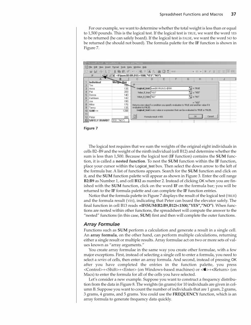
For our example, we want to determine whether the total weight is less than or equalto 1,500 pounds. This is the logical test. If the logical test is TRUE, we want the word YES

to be returned (he can safely board). If the logical test is FALSE, we want the word NO tobe returned (he should not board). The formula palette for the IF function is shown inFigure 7.

The logical test requires that we sum the weights of the original eight individuals incells B2–B9 and the weight of the ninth individual (cell B12) and determine whether thesum is less than 1,500. Because the logical test (IF function) contains the SUM func-tion, it is called a nested function. To nest the SUM function within the IF function,place your cursor within the Logical_test box. Then select the down arrow to the left ofthe formula bar. A list of functions appears. Search for the SUM function and click onit, and the SUM function palette will appear as shown in Figure 3. Enter the cell rangeB2:B9 as Number 1, and cell B12 as number 2. Instead of clicking OK when you are fin-ished with the SUM function, click on the word IF on the formula bar; you will bereturned to the IF formula palette and can complete the IF function entries.

Notice that the formula palette in Figure 7 displays the result of the logical test (TRUE)and the formula result (YES), indicating that Peter can board the elevator safely. Thefinal function in cell B13 reads =IF(SUM(B2:B9,B12)<1500,”YES”,”NO”). When func-tions are nested within other functions, the spreadsheet will compute the answer to the“nested” functions (in this case, SUM) first and then will complete the outer functions.

Array FormulaeFunctions such as SUM perform a calculation and generate a result in a single cell.An array formula, on the other hand, can perform multiple calculations, returningeither a single result or multiple results. Array formulae act on two or more sets of val-ues known as “array arguments.”

You create array formulae in the same way you create other formulae, with a fewmajor exceptions. First, instead of selecting a single cell to enter a formula, you need toselect a series of cells, then enter an array formula. And second, instead of pressing OKafter you have completed the entries in the function palette, you press<Control>+<Shift>+<Enter> (on Windows-based machines) or <>+<Return> (onMacs) to enter the formula for all of the cells you have selected.

Let’s consider a new example. Suppose you want to construct a frequency distribu-tion from the data in Figure 8. The weights (in grams) for 10 individuals are given in col-umn B. Suppose you want to count the number of individuals that are 1 gram, 2 grams,3 grams, 4 grams, and 5 grams. You could use the FREQUENCY function, which is anarray formula to generate frequency data quickly.

Spreadsheet Functions and Macros 37

Figure 7

The column labeled “Bins” in Figure 8 tells Excel how you want your data grouped.You can think of a bin as a bucket in which specific numbers go. The bins may be verysmall (hold a single or a few numbers) or very large (hold a large set of numbers). Inthis case, the numbers 1 through 5 represent the bins, and each bin “holds” just a sin-gle number. The task now is to have the spreadsheet count the number of individualsin each bin and return the answer in cells D2–D6. Because the frequency function is anarray function, we need to select cells D2–D6 (rather than a single cell) before using thefx button to summon the FREQUENCY formula.

The FREQUENCY formula palette will appear (Figure 8) and will guide you throughthe entries. The Data_array is simply the data you want to summarize, given in cellsB2:B11. The Bins_array is cells C2:C6. Instead of clicking OK, press<Control>+<Shift>+<Enter> on Windows machines, or <>+<Return> on Macs, andthe spreadsheet will return your frequencies.If we examine the formulae in cells D2–D6,every cell will have the formula {=FREQUENCY(B2:B11,C2:C6)}. The { } symbols indi-cate that the formula is part of an array.

Typically, frequency data are depicted graphically as shown in Figure 9. If you changethe data set in some way, the spreadsheet will automatically update the frequencies. Iffor some reason you get “stuck” in an array formula, just hit the Escape key and startagain.

MACROSAs noted in the Introduction (p. 16), a macro is a miniature program that you build foryourself in order to run a sequence of spreadsheet actions. Typing and mouse-clicking

38 Exercise 2

Figure 8

Figure 9

your way through a long series of commands over and over is time-consuming, boring,and error-prone. A macro allows you to achieve the same results with a single command.

You record a macro using Excel’s built-in macro recorder. Start the recorder by open-ing Tools | Macro | Record New Macro (Figure 10).

The program will prompt you to name the macro and create a keyboard shortcut.Then a small window will appear with the macro recorder controls (Figure 11). If thisbutton does not appear, go to View | Toolbars | Stop Recording, and the Stop Recording fig-ure will appear. The square on the left side of the button is the Stop Recording button.When you press this square, you will stop recording your macro. The button on the rightis the Relative Reference button. By default this button is not selected so that your macrorecorder assumes that the cell references you make in the course of developing yourmacro are absolute. In other words, if you select cell A1 as part of a macro, Excel willinterpret your keystroke as cell $A$1. There are cases (for example, the Survival Analy-sis exercise) in which you will want to select the relative reference button as you recordyour macro.

Once you have entered the macro name and shortcut key, the spreadsheet will recordevery action you take. Carry out the entire sequence of operations you want the macro

Spreadsheet Functions and Macros 39

Figure 10

Figure 11

Relative Reference buttonStop Recording button

to do, and then press the Stop Recording button in the macro recorder control window.From this point on, Excel will mimic that entire sequence of actions whenever you pressthe keyboard shortcut or issue the macro command.

PROCEDURES

Now that you have been introduced to simple functions, nested functions, arrays,and macros, it’s time to put them into practice. The following instructions will intro-duce you to some 20 commonly used spreadsheet functions. As in Exercise 1, the left-hand column of instructions gives rather generic directions, and the right-hand columngives a step-by-step breakdown of these and explanatory comments or annotations.Try to think through and carry out the instructions in the left-hand column before refer-ring to the right-hand column for confirmation. It’s tempting to jump to the right handcolumn for the answers and explanation, but you will learn a lot more about usingspreadsheet functions if you attempt it on your own. As always, save your work fre-quently to disk.

ANNOTATIONINSTRUCTIONS

A. Set up the spread-sheet.

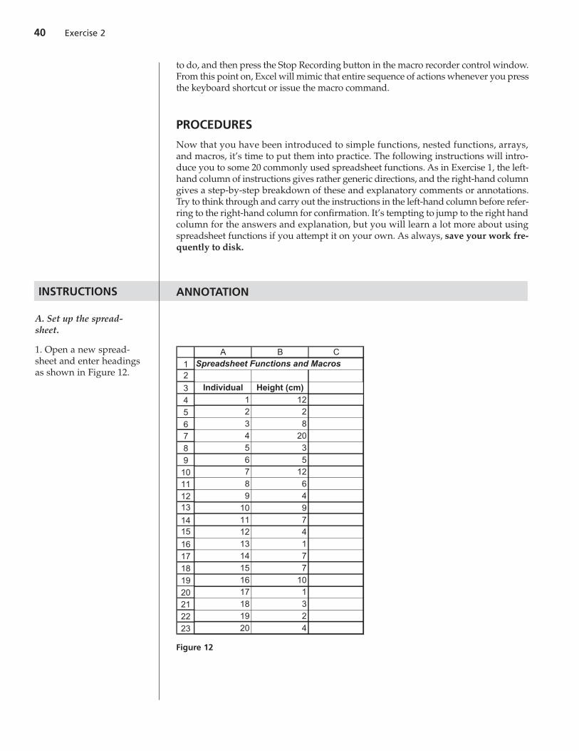
1. Open a new spread-sheet and enter headingsas shown in Figure 12.

40 Exercise 2

12

3456789

10111213

1415

1617181920212223

A B CSpreadsheet Functions and Macros

Individual Height (cm)

1 122 23 84 205 36 57 128 69 4

10 911 712 413 114 715 716 1017 118 319 220 4

Figure 12

We will consider a sample of 20 individuals and their heights. Enter 1 in cell A4.Enter =1+A4 in cell A5.Select cell A5 and copy it down to cell A23.

These are the actual data, so just type in the numbers as shown in Figure 12.

In this section, you’ll use 11 standard spreadsheet functions to compute various things,like the average height of the 20 individuals. For all functions, use the Paste Functionmenu (the Paste Function button, fx, or open Insert | Function) to locate the appropriatefunction, review the function’s formula palette, and complete the entries. You can dou-ble-check your results with ours at the end of the section.

The COUNT function counts the number of cells that contain numbers. In this case,you want to count the number of times that a number is contained in cells B4–B23.Select the COUNT function from the Paste Function menu and compute this result.After you are finished, cell E5 should display the number 20, and its formula shouldbe =COUNT(B4:B23).

For each formula, use the Paste Function menu and read through the information on theformula palette carefully. If you are unsure of the kind of information a statistic pro-vides, click on the question mark on the bottom-left corner of the formula palette. Afteryou have finished, the formulae in your spreadsheet should look like Figure 14, exceptthat instead of seeing the formula in cells E5–E12, the answers to each formula will bedisplayed.

2. Set up a linear seriesfrom 1 to 20 in cellsA4–A23.

3. Enter the heights for the20 individuals in cellsB4–B23 as shown.

B. Compute simple func-tions.

1. Set up new headings asshown in Figure 13.

2. In cell E5, use theCOUNT spreadsheet func-tion to count the totalnumber of individuals inthe sample.

3. In cells E6–E12, use thespreadsheet functionsSUM, AVERAGE, MEDI-AN, MODE, MIN, MAX,and STDEV to computebasic descriptive statisticsfor the population.

Spreadsheet Functions and Macros 41

3456789

10111213

1415

D E

CountSumAverageMedianModeMinMaxStdev4th largeRandRandbetween

Simple functions

Figure 13

The LARGE function returns the kth largest value in a range of cells. In this case, therange of cells is B4–B23 (Figure 12), and k = 4. Your formula should read=LARGE(B4:B23,4), and the answer should be 10.

You will use the RAND function in many of the exercises in this book. This functionhas the form =RAND(). The ( and ) are open and closed parentheses; you do not needto put anything inside them.

The RANDBETWEEN function generates a random integer between two specified val-ues. The bottom value is the lowermost integer that can be randomly selected (1), andthe top value is the uppermost integer that can be randomly selected (20). This func-tion could be used to randomly select an individual from the population. The for-mula in cell E15 should read =RANDBETWEEN(A4,A23) or =RANDBETWEEN(1,20).

Note: If your spreadsheet doesn’t have the RANDBETWEEN function, you can enterthe nested functions =ROUNDUP(RAND()*20,0). This will generate a random num-ber between 0 and 1, multiply it by 20, and round it up to the nearest zero decimalplaces (i.e., to the nearest integer).

The Calculate key in Windows is the F9 key, located at the top of your keyboard.* Whenthis button is pushed, the spreadsheet will recalculate all of the formulae in the spread-sheet. For random numbers, such as those generated by the RAND or RANDBE-TWEEN functions, a new random number will be generated when the spreadsheet iscalculated. Verify this by examining the results in cells E14–E15 each time you press F9.

Now we will turn to nested functions and multi-step functions. Multi-step functionsare actually standard functions like SUM, MIN, and MAX, but there are more entriesinvolved in the formula palette. A function is nested if it uses more than one functionto complete the calculations.

4. In cell E13, use theLARGE function to com-pute the fourth largestheight.

5. In cell E14, use theRAND formula to gener-ate a random numberbetween 0 and 1.

6. In cell E15, use theRANDBETWEEN func-tion to generate a randomnumber between 1 and 20.

7. Press F9, the Calculatekey, to generate new ran-dom numbers in cells E14and E15.

8. Save your work.

C. Compute multistepand nested functions.

42 Exercise 2

3456789

101112

D E

Count =COUNT(B4:B23)Sum =SUM(B4:B23)Average =AVERAGE(B4:B23)Median =MEDIAN(B4:B23)Mode =MODE(B4:B23)Min =MIN(B4:B23)Max =MAX(B4:B23)Stdev =STDEV(B4:B23)

Simple functions

Figure 14

*The F9 function key will work on Macintosh machines provided the Hot Function Keyoption in the Keyboard Control dialog box is turned OFF. If the F9 key does not work onyour Mac, use the alternative, +=.

We use the COUNTIF formula extensively. It counts the number of times a specificvalue occurs within a range of cells. Your formula should read =COUNTIF(B4:B23,E9)in cell G5, and your result should be 3, indicating that 3 individuals are 4 cm. in height.

The AND function returns the word TRUE or FALSE. It returns the word TRUE if all ofthe arguments in the formula are true (cell B4 = 12 and cell B5 = 2). If either conditionis not true, the spreadsheet returns the word FALSE. Your result should be TRUE.

The OR function is similar to the AND function in that it returns the word TRUE or FALSE.It returns the word TRUE if any of the arguments in the formula are true (cell B5 = 1 orcell B5 = 2). Your result should be TRUE.

The CONCATENATE function joins several text strings into a single text string. Theformula =CONCATENATE(F6,F7) should return the word “AndOr.” This doesn’tmean anything, but serves to illustrate the function. We will use this function in manyof the genetics exercises. (The formula =F6&F7 would generate the same result.)

The VLOOKUP function searches in the first column of a table for a value that youspecify and returns the value of the corresponding cell in a different column. TheVLOOKUP function needs three pieces of information: the value you want to find inthe first column of the table, the cells that define the table (the upper-left and lower-right cells of the table), and the number of the column in the table that holds theinformation you want the formula to return. The formula =VLOOKUP(1,A4:B23,2)looks for the number 1 in the first column of the table defined by cells A4–B23, and itreturns the value of the cell from the same row in the second column. In our spread-sheet, this formula returns the height of individual 1.

The NORMINV function is used extensively throughout the book, and is describedmore fully in Exercise 3, “Statistical Distributions.” Since here you will use the RANDfunction within the NORMINV function, this is a nested formula. Generally speak-ing, for a set of normally distributed data, the function will generate a data value if youspecify a probability associated with a normal curve. The function in cell G10 shouldread =NORMINV(RAND(),E7,E12). In this case, we will first generate a random prob-ability between 0 and 1. This probability will be applied to a normal distribution whose

1. Set up new headings asshown in Figure 15.

2. In cell G5, use theCOUNTIF formula tocount the number of timesthe modal value (given incell E9) occurs.

3. In cell G6, use the ANDfunction to determine if thevalue in cell B4 = 12 and thevalue in cell B5 = 2.

4. In cell G7, use the ORfunction to determine ifthe value in cell B5 iseither 1 or 2.

5. In cell G8, use the CON-CATENATE function tojoin the text in cell F6 withthe text in cell F7.

6. In cell G9, use theVLOOKUP function toreturn the height of indi-vidual 1.

7. In cell G10, use theNORMINV function todraw a random data pointfrom a distribution whosemean is given in cell E7,and whose standard devi-ation is given in cell E12.

Spreadsheet Functions and Macros 43

3456789

10111213

F G

CountifAndOrConcatenateVlookupNorminvRoundIfRandom height

nested functionsMulti-step and

Figure 15

mean is given in cell E7 and whose standard deviation is given in cell E12. The spread-sheet will then return the data value associated with that probability. Note when youpress F9, the Calculate key, a new random number is computed, and thus a new ran-dom data point from the normal distribution is drawn. Also note that occasionally anegative number will appear. This is because the mean is close to 0 (6.35) and thestandard deviation is quite large (4.65), so some of the data points within this distri-bution are below 0.

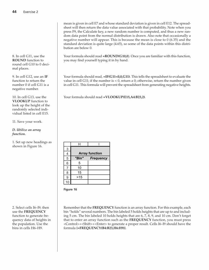
Your formula should read =ROUND(G10,0). Once you are familiar with this function,you may find yourself typing it in by hand.

Your formula should read, =IF(G11<0,0,G11). This tells the spreadsheet to evaluate thevalue in cell G11; if the number is < 0, return a 0; otherwise, return the number givenin cell G11. This formula will prevent the spreadsheet from generating negative heights.

Your formula should read =VLOOKUP(E15,A4:B23,2).

Remember that the FREQUENCY function is an array function. For this example, eachbin “holds” several numbers. The bin labeled 5 holds heights that are up to and includ-ing 5 cm. The bin labeled 10 holds heights that are 6, 7, 8, 9, and 10 cm. Don’t forgetthat to enter an array function such as the FREQUENCY function, you must press<Control>+<Shift>+<Enter> to generate a proper result. Cells I6–I9 should have theformula {=FREQUENCY(B4:B23,H6:H9)}.

8. In cell G11, use theROUND function toround cell G10 to 0 deci-mal places.

9. In cell G12, use an IFfunction to return thenumber 0 if cell G11 is anegative number.

10. In cell G13, use theVLOOKUP function tolook up the height of therandomly selected indi-vidual listed in cell E15.

11. Save your work.

D. Utilize an array function.

1. Set up new headings asshown in Figure 16.

2. Select cells I6–I9; thenuse the FREQUENCYfunction to generate fre-quency data of heights inthe population. Use thebins in cells H6–H9.

44 Exercise 2

3456789

10

H I

"Bin" Frequency

51015

>15

Array function

Figure 16

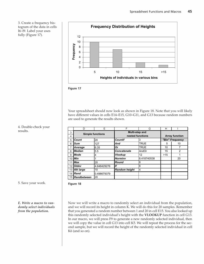
Your spreadsheet should now look as shown in Figure 18. Note that you will likelyhave different values in cells E14–E15, G10–G11, and G13 because random numbersare used to generate the results shown.

Now we will write a macro to randomly select an individual from the population,and we will record its height in column K. We will do this for 20 samples. Rememberthat you generated a random number between 1 and 20 in cell E15. You also looked upthis randomly selected individual’s height with the VLOOKUP function in cell G13.In our macro, we will press F9 to generate a new randomly selected individual, thenwe will copy the value in cell G13 into cell K5. We will repeat the process for the sec-ond sample, but we will record the height of the randomly selected individual in cellK6 (and so on).

3. Create a frequency his-togram of the data in cellsI6–I9. Label your axesfully (Figure 17).

4. Double-check yourresults.

5. Save your work.

E. Write a macro to ran-domly select individualsfrom the population.

Spreadsheet Functions and Macros 45

Frequency Distribution of Heights

0

2

4

6

8

10

12

5 10 15 >15

Heights of individuals in various binsF

req

uen

cy

Figure 17

3

4

56

7

8

910

11

1213

1415

D E F G H I

Count 20 Countif 3 "Bin" FrequencySum 127 And TRUE 5 10

Average 6.35 Or TRUE 10 7Median 5.5 Concatenate AndOr 15 2Mode 4 Vlookup 12 >15 1Min 1 Norminv 8.418740538 20

Max 20 Round 8

Stdev 4.648429276 If 84th large 10 Random height 4Rand 0.498679379Randbetween 20

Simple functionsArray functionnested functions

Multi-step and

Figure 18

There are many ways you can construct a macro to complete the task; here is one sug-gestion.

• Open Tools | Options | Calculation, and set the Calculation key to manual.• Open Tools | Macro | Record New Macro. A dialog box will appear.• Enter in a macro name (such as Sample) and a shortcut key (such as

<Control>+<t>).• If the Stop Recording button does not appear, open View | Toolbars | Stop

Recording. You should now see the Stop Recording toolbar on your spreadsheet.The filled square on the left is the Stop Recording button. Press this button withyour mouse when you are finished recording your macro.

• Press F9, the calculate key, to generate a new randomly selected individual.• Select cell G13, the height of the randomly selected individual, and open Edit |

Copy.• Select cell K4, the top row of the height column.• Open Edit | Find. A dialog box will appear (Figure 21).

1. Set up new headings asshown in Figure 19.

2. Write a macro to recordthe heights of 20 randomlysampled individuals fromthe population.

46 Exercise 2

3456789

10111213

1415

16171819202122232425

J K

Sample Height

1234567891011121314151617181920

average

Macro

Figure 19

• Leave the box labeled Find What blank, and select the Search By Columns option.Click on Find Next, then on Close. Your cursor should have moved down to thenext empty cell on your spreadsheet.

• Open Edit | Paste Special, and select the Paste Values option. Click OK.• Click on the Stop Recording button.

That’s all there is to it. Now when you press the shortcut key, <Control>+<t>, thespreadsheet will repeat the steps in the macro automatically. Run your macro until youhave obtained the heights of 20 randomly sampled individuals. (Note that with thisprocess, the same individuals can be sampled more than once.)

You can view the code that the spreadsheet “wrote” as a result of your keystrokes bygoing to Tools | Macros | Macro. Select the macro name of interest, and click on Edit. TheVisual Basic code will be revealed. When you are finished, click on the x button in theupper-right hand corner of the spreadsheet to close the Visual Basic code. You will bereturned to your original spreadsheet.

You may want to switch your calculation key back to automatic; otherwise, you mustpress F9 any time you want your spreadsheet to calculate values.

QUESTIONS

1. Explore the formulae used in the exercise by changing some of the heights ofthe individuals. For example, change cell B5 from 2 to 1. How does this changeaffect the outcome of the AND and OR functions? Change other values in thedata set as well. How do your changes affect the frequency distribution of thedata?

2. Click on the Paste Function button, fx, and select the function category ALL. A listof all functions is displayed on the right-hand side of the Paste Function dialogbox. Click on a function that looks interesting, and notice the description of thefunction that appears in the lower portion of the dialog box. Select three functionsthat were not used in this exercise and explore how each function works. Choosefunctions that are likely to be relevant to the data set in the exercise.

3. Save your work.

Spreadsheet Functions and Macros 47

Figure 20