) 2017... · ANGRAU/July 2017 Regd. No. 25487/73 Printed at Ritunestham Press, Guntur and Published...
133
THE JOURNAL OF RESEARCH ANGRAU ACHARYA N.G. RANGA AGRICULTURAL UNIVERSITY Lam, Guntur - 522 034 The J. Res. ANGRAU, Vol. XLV No. (2), pp 1-130, April-June, 2017 Indexed by CAB International (CABI) www.cabi.org and www.angrau.ac.in ISSN No. 0970-0226
-
Upload
trinhkhuong -
Category
Documents
-
view
219 -
download
0
Transcript of ) 2017... · ANGRAU/July 2017 Regd. No. 25487/73 Printed at Ritunestham Press, Guntur and Published...

ANGRAU/July 2017 Regd. No. 25487/73
Printed at Ritunestham Press, Guntur and Published by Dr. R. Veeraraghavaiah, Dean, P.G. Studies and Editor,The Journal of Research ANGRAU, Acharya N.G. Ranga Agricultural University, Lam, Guntur - 522 034
E-mail : [email protected], www.angrau.ac.in/publications
THE JOURNAL OFRESEARCHANGRAU
ACHARYA N.G. RANGA AGRICULTURAL UNIVERSITY
Lam, Guntur - 522 034The J. Res. ANGRAU, Vol. XLV No. (2), pp 1-130, April-June, 2017
Indexed by CAB International (CABI)www.cabi.org and www.angrau.ac.in
The J. Res. A
NG
RA
U, Vol. XLV N
o. (2), pp 1-130, April-June, 2017
ISSN No. 0970-0226
SUBSCRIPTION TARIFF
Individual (Annual) : Rs 300/- Institutional (Annual) : Rs. 1200/-Individual (Life) : Rs. 1200/- Printing Charges : Rs. 100/- per page
DD drawn in favour of COMPTROLLER, ANGRAU, GUNTUR may be sent to the Principal Agricultural Information Officer,Agricultural Information & Communication Centre, E.S.R. Enclave, Balaji Nagar, M.G. Inner Ring Road, Guntur - 522 509, A.P.
RESEARCH EDITOR : Dr. A. Lalitha, AI & CC, E.S.R. Enclave, Balaji Nagar, M.G. Inner Ring Road, Guntur - 522 509
EDITORDr. R. Veeraraghavaiah
Dean of P.G. StudiesAdministrative Office, ANGRAU, Guntur
MANAGING EDITORDr. P. Punna Rao
Principal Agricultural Information Officer,AI & CC, Guntur - 522 509
The Journal of Research ANGRAU(Published quarterly in March, June, September and December)
ADVISORY BOARD
EDITORIAL COMMITTEE MEMBERS
Dr. T. Ramesh BabuDean of Agriculture
Dr. T. NeerajaDean of Home Science
Dr. R. Sarada Jayalakshmi DeviUniversity Librarian
Dr. N. V. NaiduDirector of Research
Dr. R. VeeraraghavaiahDean of P.G. Studies
Dr. P. Sambasiva RaoDean of Students Affairs
Dr. A Subramanyeswara RaoNodal Officer
Dr. K. Raja ReddyDirector of Extension
Dr. D. Bhaskara RaoDean of Agricultural Engineering &Technology
Dr. A. Siva SankarController of Examinations
Dr. G. Sunil Kumar BabuCoordinator (Polytechnics)
Dr. R. Ankaiah (Crop Physiology), Naira
Dr.D. Anitha (Apparel & Textiles), Guntur
Dr. D. Bala Guravaiah (Soil Science & Agril. Chemistry), Mahanandi
Dr. C.P. Dorai Rajan (Plant Pathology), Nellore
Dr. N.P. Eswara Reddy (Plant Molecular Biology & Bio Technology), Tirupati
Dr. B. Gopal Reddy (Agronomy), Nandyala
Dr. B. Govinda Rao (Genetics & Plant Breeding), Guntur
Dr. B. John Wesley (Agro Energy), Bapatla
Dr. P.V. Krishnayya (Entomology), Bapatla
Dr. (Mrs) J. Lakshmi (Foods & Nutrition), Guntur
Dr. B.V.S. Prasad (Food Science & Technology), Bapatla
Dr. M. Raghu Babu (Soil and Water Engineering), Guntur
Dr. C. Ramana (Farm Machinery and Power), Mahanandi
Dr. P. Rambabu (Agricultural Extension), Bapatla
Dr. Ch.V.V. Satyanarayana (Food Engineering), Bapatla
Dr. Sivala Kumar (Agricultural Process and Food Engineering), Bapatla
Dr. V. Srinivasa Rao (Statistics), Bapatla
Dr. V. Srilatha (Horticulture), Tirupati
Dr. N. Trimurthulu (Agricultural Microbiology), Amaravati
Dr. L. Uma Devi (Human Development and Family Studies), Guntur
Dr. D. Vishnu Sankar Rao (Agricultural Economics), Guntur

CONTENTS
PART I: PLANT SCIENCES
Genetic behaviour of bacterial wilt resistance in F2 population of brinjal (Solanum melongena L.) 1G. M. KURHADE, S.G. BHAVE, S.V. SAWARDEKAR, M. M. BURONDKAR and V.V. DALVI
Inheritance pattern of the dwarf gene controlling plant height in rice 6K. GOPALA KRISHNA MURTHY, N. RANJITH KUMAR, V.L.N. REDDY, A. SRIVIDHYA,P.V. SATYANARAYANA, P.V. RAMANA RAO, M. SHESHU MADHAV and E.A. SIDDIQ
Effect of plant geometry and fertilizer levels on yield and yield attributes and 14quality character of cowpea (Vigna unguiculata L. Walp)A.R. JAGADALE, G.K.BAHURE, G.R. LAHANE, I.A.B. MIRZA and S.R.GHUNGARDE
Bio efficacy of different biorational insecticides for the management of 19spotted stem borer, Chilo partellus (Swinhoe) in maize (Zea mays L.)G.V. SUNEEL KUMAR, T.MADHUMATHI, D.V. SAIRAM KUMAR,V.MANOJ KUMAR and M. LAL AHAMAD
Micro level climatic classification of Ananthapuramu district of Andhra Pradesh 31S. MALLESWARI, G.NARAYANA SWAMY, A.B.SRINATH REDDY, K.C. NATARAJ,B. SAHADEVA REDDY and B. RAVINDRANATHA REDDY
Comparision of extractants to assess potassium availability in soils of 38major cropping systems in Kurnool districtI.RAJEEVANA, P.KAVITHA, M.SREENIVASA CHARI and M.SRINIVASA REDDY
Yield and economics of maize-chickpea sequence as influenced by 50sowing time and nitrogen levelsM. RATNAM, B. VENKATESWARLU, E. NARAYANA, T.C.M NAIDU andA. LALITHAKUMARI
Effect of urban compost application to soil on ground water quality 59V. RAMBABU NAIK, P. PRABHU PRASADINI and V. SAILAJA
Weed Management with pre and post emergence herbicides in maize 64A. SUBBARAMIREDDY, A. S. RAO, G. SUBBA RAO, T .C. M. NAIDU,A. LALITHA KUMARI and N. TRIMURTHULU

PART II: SOCIAL SCIENCES
Generating market information and market outlook of major cassava markets in 75Africa: A direction for Nigeria trade investment and policyM. S. SADIQ, I.P SINGH, I.J. GREMA, S.M. UMAR and M.A. ISAH
Conservation of traditional rice varieties for crop diversity in Kerala 93P. INDIRA DEVI, SEBIN SARA SOLOMON and MRIDULA NARAYANAN
Marketing efficiency and market competitiveness of farmer producer companies 100(FPCs) - A case of Telangana and Karnataka statesM.KANDEEBAN and Y.PRABHAVATHI
Knowledge mapping on rice (Oryza sativa L.) production technologies 108by the farmers of Karimnagar district in Telangana StateN. VENKATESHWAR RAO, P.K. JAIN, N. KISHORE KUMAR andM. JAGAN MOHAN REDDY
PART III: RESEARCH NOTES
Inter temporal variations in sex ratio in India: state wise analysis 117P.KANAKA DURGA
1
INTRODUCTION
The brinjal or eggplant or aubergine (Solanummelongena L.) represents the non-tuberous group ofSolanum species. Brinjal is the most common,popular and widely grown vegetable crop of bothtropics and subtropics of the world. Brinjal usuallyfinds its place as the poor man’s vegetable (Somand Maity, 2002). Except in higher altitudes, it canbe grown in almost all parts of India, all the yearround. Large number of cultivars is grown throughoutthe country depending upon the consumer’spreference for the colour, size, shape and the yieldare specific which changes with region. In India,immature fruits of brinjal are consumed as cookedvegetable in various ways. Growth and productivityof brinjal plant is hampered by serious diseases likebacterial wilt (BW).
Recently, this disease rose to alarmingproportion in the plains of India and has become oneof the limiting factors. The bacterial wilt is causedby Ralstonia solanacearum (Smith). Yabuchi et al.(1995) reported that it causes yield loss ranging from4.24 to 86.14 per cent. The race I of Ralstoniasolanacearum infects almost all solanaceous crops.Source of resistance to bacterial wilt has beenreported by many workers viz., SM132, SM6-2, SM6-6, SM6-7 (Geetha and Peter, 1993), IHR-171, IHR-
GENETIC BEHAVIOUR OF BACTERIAL WILT RESISTANCE IN F2 POPULATIONOF BRINJAL (Solanum melongena L.)
G. M KURHADE., S. G. BHAVE, S. V. SAWARDEKAR, M. M. BURONDKAR AND V. V. DALVICollege of Agriculture, Dr. Balasaheb Sawant Konkan Krishi Vidyapeeth, Dapoli- 415712
Date of Receipt: 06.3.2017 Date of Acceptance:25.4.2017
ABSTRACTBrinjal or eggplant (Solanum melongena L.) is severely affected by bacterial wilt caused by Ralstonia solanecearum
in Konkan Region of Maharashtra. Resistant varieties are most suitable option to reduce crop losses from bacterial wilt. Theknowledge of resistance mechanism and its inheritance is important to develop resistant varieties. Thus, the present study wasconducted during rabi 2015-16 to understand the genetic behaviour of bacterial wilt resistance in brinjal. For this study, the fiveF2 population which were chosen by 15 F1 hybrids derived from line x tester crosses of three female x five male parents. Theexperiment was carried out in naturally bacterial wilt affected plot available at Research Farm, Department of Agricultural Botany,College of Agriculture, Dapoli. It could be inferred that the inheritance of bacterial wilt resistance in brinjal plants under conditionof naturally bacterial wilt infested soil was quantitative (polygenic) in nature.
E-mail: [email protected]
J.Res. ANGRAU 45(2) 1-5, 2017
180, IHR-181, IHR- 182, IHR-85 (Sadashiva et al.,1994), Arka Nidhi, Arka Keshav, Arka Neelkantha,BB1, BB44, BB49, EP143, Surya, BB 13-1, BB2,Kerala local, SM6-6 (Ponnuswami, 1999). The wildbrinjal S. melongena var. insanum (Srinivasan andGopimony, 1969) and Solanum torvum SW (Goussetet al., 2005) are resistant against R. solanacearum,but till today resistance to bacterial wilt in many localgermplasms is not known.
At present, most of the commercially grownvarieties of brinjal are susceptible to bacterial wiltwhich is a limiting factor for successful cultivation ofthis crop in the areas having high temperature andhumidity during rainy season. Sometimes, there isa complete failure of crop, thereby resulting in hugeeconomic losses to the vegetable growers. Thechemical control of the disease involves hugeexpenditure and cumbersome too. The knowledgeon genetics of resistance helps in the formulation ofthe breeding method. Therefore, development ofresistant varieties suitable for Konkan region is mosteconomic, eco-friendly and feasible method toensure better productivity of brinjal. Therefore, thepresent study was undertaken to understand thegenetic behaviour of bacterial wilt of brinjal in Konkanconditions.

2
MATERIAL AND METHODS
Out of 15 F1 hybrids, five F1s viz, M. Gota ×BB-54, Malapur × BNDT, BR-14 × BNDT, BR-14 ×PPC and BR-14 x Kasral were selfed based on theirperformance and resistance towards the wilt duringrabi 2014-15 to get F2 population. Above Five F2
population, with their F1s and their respective parentsand resistant standard check (Swarna Pratibha) wereused for the study of bacterial wilt inheritance. Eachcross-involved bacterial wilt resistant genotypes (BB54, BNDT, PPC and Kasral) as one of the parents,whereas, other parent involved in the crossrepresented commercial but susceptible cultivars(Manjari Gota, Malapur and BR-14). Forty days oldseedlings were transplanted in the naturally sick plotavailable at research farm of Agricultural Botany,Dapoli during rabi 2015-16. Separate blocks weremade for parents, F1 and F2 population. Each F2
population consisted of 500 plants excepted BR-14x BNDT had 438 while parents, check and F1 had apopulation of 15 plants each. Recommended packageof practices were followed for raising the crop. Thewilted plants were counted 90 days after transplanting(DAT) and final count was taken for calculating theinheritance pattern.
Observations were recorded on individualplant basis. A plant is considered as resistant tobacterial wilt if it doesn’t wilt. The whole F2 populationwas categorized into wilted and non-wilted populationto know the genetics of resistance. The genetic ratioswere tested based upon goodness of fit forinheritance using chi-square test.
RESULTS AND DISCUSSION
The experimental results obtained on theinheritance of bacterial wilt resistance in F2
populations are given in Table 1. In the present study,the cross Mlp x BNDT the segregation of F2s was inthe ratio of 3(R):1(S) which suggested monogenicinheritance of resistance while in the crosses Mgt xBB 54 and BR 14 x PPC, a segregation of 9:7 ofresistant and susceptibility were observed, indicating
that the resistance was governed by complementarygene interaction. Whereas, in the crosses BR 14 xBNDT and BR 14 x Kasral, the segregation in F2
progenies did not fit to mono or di-genic ratiosindicating that the resistance was controlled bypolygene. Single dominant gene for resistance tobacterial wilt has also been reported in brinjal byChaudhary and Sharma (1999), Ajjappalavara et al.(2008) and Bi-hao et al. (2009).
Ooze test was carried out to ensure thedeath of plants due to bacterial wilt. Fig. 1 and Fig.2 show that microscopic slide of bacterial ooze outfrom roots of wilted plant at 30 and 60 DAT,respectively. Fig. 3 indicates that confirmation ofbacterial wilt disease by regular testing of wilted plantthrough ooze test. All the plants showing wiltingsymptoms were subjected to ooze test up to finalcount 90 days after transplanting (DAT).
In literature, variable reports on the genetics/inheritance of bacterial wilt resistance in varioussolanaceous vegetable crops have been reported.The parental lines used in this study were differentfrom those of earlier workers and this variation alongwith differences in the strains of the pathogen anddifferent environmental conditions of study mayperhaps be the reason for the difference in results.Chaudhary (2000) has reported variable segregationpatterns ranging from monogenic dominant andrecessive to inhibitory type in different cross-combinations of brinjal. Neto et al. (2002) reportedthat inheritance of resistance to bacterial wilt intomato plants is quantitative with partial dominanceof the alleles. Linlin et al. (2003) concluded that theinheritance of bacterial wilt resistance as additive-dominant model in brinjal while bacterial wiltresistance was controlled by number of minor, majorand cytoplasmic genes. Sharma and Sharma (2015)observed that there is a significant role of additiveand dominance components and their interactionsin the expression of bacterial wilt resistance intomato. Bainsla et al. (2016) revealed that there waspreponderance of recessive gene family wherein morethan one gene acts in additive mode in brinjal.
KURHADE et al.

3
1 Mgt x BB54 Resistant 270 230 3 : 1 117.6* 3.84 Complementary(9:7)
2 Mlp x BNDT Resistant 393 107 3 : 1 3.46NS 3.84 Monogenicdominant(3:1)
3 BR14 x BNDT ModeratelySusceptible 182 256 3 : 1 261.34* 3.84 ?
4 BR14 x PPC Moderately ComplementarySusceptible 279 221 3 : 1 98.30* 3.84 (9:7)
5 BR14 x Kasral ModeratelySusceptible 184 316 3 : 1 389.13* 3.84 ?
F2
Observed frequencyExpected
Ratio(R:S)
X2value(Calu-
clated)
X2 value(Table)
Type ofgene
actionResistant Susceptible
Table 1. Mode of inheritance of bacterial wilt resistance in F2 population of brinjal
S.No. Crosses F1
BACTERIAL WILT RESISTANCE IN BRINJAL

4
CONCLUSION
It could be concluded that the inheritance ofbacterial wilt resistance in brinjal plants undercondition of naturally bacterial wilt infested soil wasquantitative (polygenic) in nature. It shall, therefore,be more appropriate to carry out the genetics/inheritance of resistance studies under controlledconditions and inoculating the plants with knownstrain(s) of the pathogen so as to have accurateinformation.
REFERENCES
Ajjappalavara, P.S., Dharmatti, P. R., Salimath, P.M., Patil, R. V., Patil, M.S and Krishnaraj,P. U. 2008. Genetics of bacterial wiltresistance in brinjal. Karnataka Journal ofAgricultural Sciences. 21(3): 424-427.
Bainsla, N. K., Singh, S., Singh, P.K., Kumar, K. A.,Singh, K. R and Gautam, K. 2016. Genetic
behaviour of bacterial wilt resistance inbrinjal (Solanum melongena L.) in tropics ofAndaman and Nicobar Islands of India.American Journal of Plant Sciences. 7: 333-338.
Bi-hao, C., Jian-jun, L., Yong, W and Guo-ju, C. 2009.Inheritance and identification of SCARmarker linked to bacterial wilt-resistance ineggplant. African Journal of Biotechnology.8(20): 5201-5207.
Chaudhary, D. R. 2000. Inheritance of resistance tobacterial wilt (Ralstonia solanacearum E. F.Smith) in eggplant. Haryana Journal ofHorticultural Sciences. 29(1): 89-90.
Chaudhary, D.R and Sharma, D.K. 1999. Studies onbacterial wilt (Pseudomonas solanacearumE.F. Smith) resistance in brinjal. IndianJournal of Hill Farming. 12(1/2): 94-96.
KURHADE et al.

5
Geetha, P.T and Peter, K.V. 1993. Bacterial wiltresistance in a few selected lines and hybridsof brinjal (Solanum melongena L.). Journalof Tropical Agriculture. 31: 274–276.
Gousset, C., Collonnie, C., Mulya, K., Mariska, I.,Rotino, G.L., Besse, P., Servaes, A andSihachakr, D. 2005. Solanum torvum, as auseful source of resistance against bacterialand fungal diseases for improvement ofeggplant (Solanum melongena L.). PlantScience. 168: 319-327.
LinLin, F., Yu, Q. D., Ping, J. L and Yong, L. 2003.Genetic analysis of resistance to bacterialwilt (Ralstonia solanacearum) in eggplant(Solanum melongena L.). Acta HorticulturaeSinica. 30(2): 163-166.
Neto, A.F.L., Silveira, M.A., De Souza, R.M.,Nogueira, S. R and André, C.M.G. 2002.Inheritance of bacterial wilt resistance intomato plants cropped in naturally infestedsoils of the state of Tocantins. Crop Breedingand Applied Biotechnology. 2(1): 25-32.
Ponnuswami, V. 1999. Studies on bacterial wiltresistance of selected eggplant accessoriesinoculated with Pseudomonassolanacearum PSSS97 for 30 days undergrowth room conditions at Asian VegetableResearch and Development Centre.Capsicum and Eggplant Newsletter. 12: 91–93.
Sadashiva, A. T., Madhavireddy, K., Deshpande A.Aand Singh, R. 1994. Yield performance ofeggplant lines resistance to bacterial wilt.Capsicum and Eggplant Newsletter. 13: 104-106.
Sharma, K.C and Sharma, L.K. 2015. Geneticstudies of bacterial wilt resistance in tomatocrosses under mid-hill conditions ofHimachal Pradesh. Journal of Hill Agriculture.6(1):136-137.
Srinivasan, K and Gopimony, R. 1969. On theresistance of wild brinjal variety to bacterialwilt. Agricultural Research Journal of Kerala.7(1): 39-40.
Som, M.G and Maity, J.K. 2002. Vegetable Crops.Bose, T. K., Kabir, J., Maity, T. K.,Parthasarthy, V. A and Som, M. G. (Eds.)3rd Revised Edition. Naya ProkashPublishers, Kolkata. pp. 265-344.
Yabuchi, E., Kosako, Y., Yano, I., Hotta, H andNishiuchi, Y. 1995. Transfer of twoBurkholderia and Alcaligenes species toRalstonia gen nov.: proposal of Rolstoniapicketti (Ralston, Palleroni and Doudoroff,1973). comb. nov. Ralstonia eutropha (Smith,1896) comb. nov. and Ralstonia eutropha(Davis, 1969) comb. Nov. Microbiology andImmunology. 39(11): 897-904.
BACTERIAL WILT RESISTANCE IN BRINJAL

6
INTRODUCTION
Rice is the staple food for more than half ofthe world’s population. Tropical Asia, accounting forover 90% of production and consumption of rice, hadbeen cultivating low yielding, tall statured lodging-prone varieties until the advent of the non-lodginghigh yielding semi-dwarf varieties (short) in the mid-sixties. The short statured varieties, developed usingDee-Gee-Woo-Gen (DGWG), a spontaneous dwarfmutant as the donor, have enabled many countriesin the region to achieve self-sufficiency in riceproduction in a short span of 15 years (Sasaki etal., 2002 and Spielmeyer et al., 2002). The semi-dwarfism in DGWG is reported to be controlled by asingle recessive gene, sd1 (Cho et al., 1994).
The success of DGWG- based varietiessuch as IR8 and Taichung Native 1 has madebreeders all over to depend excessively on thesetwo rice cultivars as source breeds for short staturetrait. Hence, over 90% of the currently cultivated highyielding varieties have sd1 gene as dwarfing source,from DGWG source (Cho et al., 1994 and Spielmeyer
INHERITANCE PATTERN OF THE DWARF GENE CONTROLLING PLANTHEIGHT IN RICE
K. GOPALA KRISHNA MURTHY *, N. RANJITH KUMAR, V.L.N. REDDY,A. SRIVIDHYA, P.V.SATYANARAYANA, P.V. RAMANA RAO, M. SHESHU MADHAV AND E.A. SIDDIQ
Institute of Frontier Technology, Acharya N.G. Ranga Agricultural University, Tirupati –517 502
Date of Receipt: 22.5.2017 Date of Acceptance:27.6.2017
ABSTRACT
Dwarfism is a valuable trait in crop breeding, because it increases lodging resistance and decreases damages due towind and rain. The experiment (rabi 2013 to kharif 2014) aimed to study the inheritance pattern of a dwarf mutant LND384,employing different F2 progenies, developed by crossing with semi-dwarf, intermediate and tall groups. All the F1 progeny showedheterosis over their parents towards tallness, indicating dominance of the trait. However, the plant height of F2 progenies mostlyskewed towards tall parent type or either short type, with platykurtic nature. Although bimodal distribution was seen withdepression in the F2 frequency curves of three crosses, namely LND384 x MTU1010, LND384 x Swarna and LND384 x Dular, alsocouldn’t fit the expected mendalian ratio of 3:1. Hence, possibly the plant height in the dwarf derived population is controlled bymajor genes in combination with minor and/or modifier genes.
E-mail : [email protected]; * Part of PhD thesis of author
J.Res. ANGRAU 45(2) 6-13, 2017
et al., 2002). This forms the base for genetichomogeneity to high extent; render a vital characterlike plant height genetically vulnerable to suddenoutbreak of diseases and insect pests. To overcomesuch an eventuality many efforts have been madesince last three decades for broadening the geneticbase through identification and use of alternatedwarfing gene sources (Singh et al., 1979).
Genetic analysis of a large number of dwarfsof spontaneous and induced mutant origin hasrevealed that dwarfs, non-allelic to sd1 are rare.However, a dwarf source LND384 (54cm ± 1.86cm),which is non-allelic to sd1 was identified in an in-house study using sd1 gene specific markers. Inorder to precise use of the source material in thebreeding programme and to broaden the genetic basefor plant height, prior knowledge on gene action andits inheritance pattern is necessary. To understandthe genetic nature of plant height, the current studyis initiated with seven crosses involving the LND 384as dwarf parent with genotypes of diverse plant heightgroups.

7
MATERIAL AND METHODS
Seven varieties/accessions that representingsemi-dwarf (<110cm), intermediate (110-130cm) andtall (>130cm) (SES, IRRI, 2002) types were used inthe study and are crossed in the followingcombinations viz. LND384 x MTU1010 (dwarf x semi-dwarf); LND84 x Swarna (dwarf x semi-dwarf);LND384 x BPT5204 (dwarf x tall); LND384 x Dular(dwarf x tall); LND384 x Pusa1121 (dwarf x tall);LND384 x PLA1100 (dwarf x tall) and LND384 xINRC10192 (dwarf x tall) during kharif 2013. The F1swere selfed to generate F2 population during rabi 2013.
For each cross F1 (20-25 plants), F2 (100-200 plants) and parents (100 -120 plants) were grownin adjacent plots during kharif 2014 at AndhraPradesh Rice Research Institute and RegionalAgricultural Research Station, Maruteru. Plantspacing was given as 30cm x 20cm. Standard fieldmanagement practices were followed throughout thecrop growth period. The plant height was measuredfrom the base of the plant to the tip of the tallestpanicle. The phenotypic data was analyzed with dataanalysis package of MS-Excel Software, 2007version.
Confirmation of F1 Plants
Using polymorphic SSR (Simple SequenceRepeat) markers, the heterozygosity of F1 plants foreach cross were confirmed. The leaves from eachparent were collected and frozen for DNA extraction.The cetyl trimethyl ammonium bromide (CTAB)method was used to extract genomic DNA from about1.0g of young leaf tissue of each parent (Murray andThompson 1980). The quality of DNA was checkedusing 0.8% agrose gel electrophoresis, and the DNAconcentration was measured using Nanodrop reader.
The PCR reactions were carried out in 10µlvolume, which contains 50ng rice genomic DNA, 5pico moles each of forward and reverse primers, 0.1Mdeoxy nucleotide tri-phosphates (dNTPs), 1X Taq
buffer and 1U of Taq polymerase. The PCR conditionsinvolve initial denaturation at 94°C for 3 min and 35cycles of denaturation at 94°C for 45 sec followedby annealing at 54-58°C for 1 min and extension at72°C for 45 sec and a final extension at 72°C for 10min. The amplified PCR products were resolved on3% agarose gel prepared in 1X TAE buffer stainedwith 10µM ethidium bromide and the resolved PCRbands were detected using Bio Rad Molecular Imager(Gel Doc-XR System). The gels were analyzed forthe status of the genotype using SSR markers andthe F1 plants were confirmed for their heterozygosity.
RESULTS AND DISCUSSION
The study focused on characterizing anddetermining the inheritance pattern of plant heighttrait among the seven F2 populations developed fromcrosses involving a dwarf rice mutant LND384 with54cm ± 1.86cm plant height (non-allelic to sd1) asfemale parent and semi-dwarf (<110cm), intermediate(110-130cm) and tall (>130cm) genotypes as maleparents. The F1 plants were confirmed for theirheterozygosity by employing parental polymorphicSSR markers namely RM151 and RM562 (Fig. 1).The confirmed F1 plants were selfed for generation ofF2 population.
Plant height of F1 progeny
The F1 generation of all seven crosses,irrespective of their pollen parental phenotypic group(semi-dwarf/intermediate/tall), showed heterosistowards tall plant nature except the progeny ofLND384 x Swarna (Fig. 2), which is a semi-dwarftype. The inter-nodal lengths of major tiller of LND384x Swarna F1 plants showed clear demarcation of lesselongation when compared to the other crosses (Fig.2-II) and hence semi-dwarf type. Further, theinternode number also five as aginst six in othercrossess. Hence, it can be concluded that plantheight is controlled by one or more major genes,apart from minor gene effects.
GOPALA KRISHNA MURTHY et al.
8
Plant height in F2 progeny
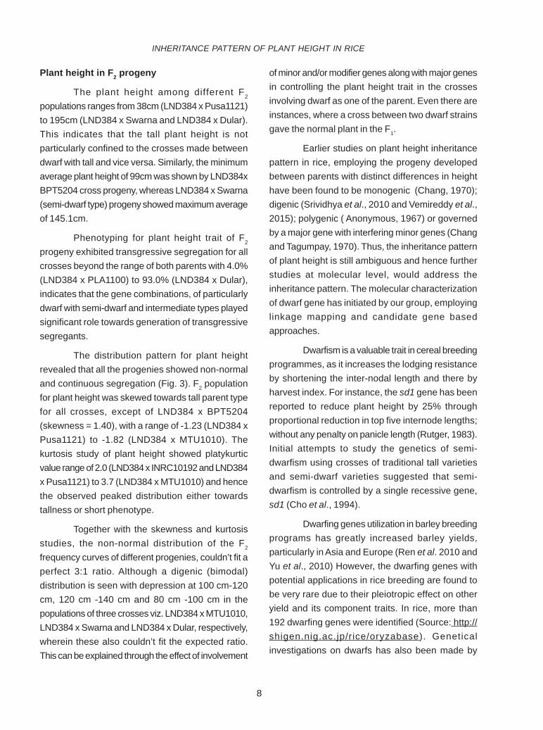
The plant height among different F2
populations ranges from 38cm (LND384 x Pusa1121)to 195cm (LND384 x Swarna and LND384 x Dular).This indicates that the tall plant height is notparticularly confined to the crosses made betweendwarf with tall and vice versa. Similarly, the minimumaverage plant height of 99cm was shown by LND384xBPT5204 cross progeny, whereas LND384 x Swarna(semi-dwarf type) progeny showed maximum averageof 145.1cm.
Phenotyping for plant height trait of F2
progeny exhibited transgressive segregation for allcrosses beyond the range of both parents with 4.0%(LND384 x PLA1100) to 93.0% (LND384 x Dular),indicates that the gene combinations, of particularlydwarf with semi-dwarf and intermediate types playedsignificant role towards generation of transgressivesegregants.
The distribution pattern for plant heightrevealed that all the progenies showed non-normaland continuous segregation (Fig. 3). F2 populationfor plant height was skewed towards tall parent typefor all crosses, except of LND384 x BPT5204(skewness = 1.40), with a range of -1.23 (LND384 xPusa1121) to -1.82 (LND384 x MTU1010). Thekurtosis study of plant height showed platykurticvalue range of 2.0 (LND384 x INRC10192 and LND384x Pusa1121) to 3.7 (LND384 x MTU1010) and hencethe observed peaked distribution either towardstallness or short phenotype.
Together with the skewness and kurtosisstudies, the non-normal distribution of the F2
frequency curves of different progenies, couldn’t fit aperfect 3:1 ratio. Although a digenic (bimodal)distribution is seen with depression at 100 cm-120cm, 120 cm -140 cm and 80 cm -100 cm in thepopulations of three crosses viz. LND384 x MTU1010,LND384 x Swarna and LND384 x Dular, respectively,wherein these also couldn’t fit the expected ratio.This can be explained through the effect of involvement
of minor and/or modifier genes along with major genesin controlling the plant height trait in the crossesinvolving dwarf as one of the parent. Even there areinstances, where a cross between two dwarf strainsgave the normal plant in the F1.
Earlier studies on plant height inheritancepattern in rice, employing the progeny developedbetween parents with distinct differences in heighthave been found to be monogenic (Chang, 1970);digenic (Srividhya et al., 2010 and Vemireddy et al.,2015); polygenic ( Anonymous, 1967) or governedby a major gene with interfering minor genes (Changand Tagumpay, 1970). Thus, the inheritance patternof plant height is still ambiguous and hence furtherstudies at molecular level, would address theinheritance pattern. The molecular characterizationof dwarf gene has initiated by our group, employinglinkage mapping and candidate gene basedapproaches.
Dwarfism is a valuable trait in cereal breedingprogrammes, as it increases the lodging resistanceby shortening the inter-nodal length and there byharvest index. For instance, the sd1 gene has beenreported to reduce plant height by 25% throughproportional reduction in top five internode lengths;without any penalty on panicle length (Rutger, 1983).Initial attempts to study the genetics of semi-dwarfism using crosses of traditional tall varietiesand semi-dwarf varieties suggested that semi-dwarfism is controlled by a single recessive gene,sd1 (Cho et al., 1994).
Dwarfing genes utilization in barley breedingprograms has greatly increased barley yields,particularly in Asia and Europe (Ren et al. 2010 andYu et al., 2010) However, the dwarfing genes withpotential applications in rice breeding are found tobe very rare due to their pleiotropic effect on otheryield and its component traits. In rice, more than192 dwarfing genes were identified (Source: http://shigen.nig.ac.jp/rice/oryzabase). Geneticalinvestigations on dwarfs has also been made by
INHERITANCE PATTERN OF PLANT HEIGHT IN RICE

9
several workers, and are reported as dominant, semi-dominant and recessive in inheritance pattern viz.,D53, Ssi1, Sdd(t), Dx, TID1, LB4D, Slr-f, D-h etc
(Mori et a1., 1973). Hence, identification of newdwarfing genes, studies on their inheritance patternand their potential practical applications in future ricebreeding is considered to be important.
GOPALA KRISHNA MURTHY et al.

10
INHERITANCE PATTERN OF PLANT HEIGHT IN RICE

11
GOPALA KRISHNA MURTHY et al.

12
CONCLUSIONFrom the current study, it can be concluded
that, tall character in F1 involving a dwarfing sourceas parent, was dominant in nature. However, F2
distribution of the seven crosses although resemblescontinuous variation typical to a quantitative trait,doesn’t follow an expected mendalian ratio. Theskewness and kurtosis studies imply the involvementof many minor and/or modifier genes along with majorgenes in the control of F2 plant height, as there is alarge range of variation for plant height found in allthree phenotypic parental crosses. Hence,culmination of phenotypic studies with molecular levelapproaches would result in better understanding ofthe inheritance nature of rice dwarfing gene(s) thatcould be used in future breeding programmes.
REFERENCESAnonymous, 1967. Inheritance of short stature in U.S.
strains. Annual Report. IRRI, Los Banos,Philippines. pp69.
Chang, T.T. 1970. Genetic studies on semi-dwarf rice.Journal of Taiwan Agricultural Research.(19)4: 1-10.
Chang, T.T and Tagumpay O. 1970. Genotypicassociation between grain yield and sixagronomic traits in a cross between ricevarieties of contrasting plant type. Euphytica19 (3): 356-36.
Cho, Y.G., Eun, M.Y., Mc Couch, S.R and Chae,Y.A. 1994. The semi-dwarf gene, sd-1, of riceOryza sativa L. II. Molecular mapping andmarker-assisted selection. Theoretical andApplied Genetics. 89 (1): 54-59.
Mori, M., Kinoshita, T and Takahashi, M.E. 1973.Linkage relationships of genes for somemutant characters of rice kept in KyushuUniversity. Genetical studies of rice plant.L.II Memorial Faculty of Agricuiture.Hokkaido University. 8(4): 377-385.
Murray, M.G and Thompson, W.F. 1980. Rapidisolation of high molecular weight plant DNA.Nucleic Acids Research. 10: 4321-4325.
Ren, X., Sun, D., Guan, W., Sun, G. and ChengdaoL. 2010. Inheritance and identification ofmolecular markers associated with a noveldwarfing gene in barley. BMC Genetics. 11:
Min: minimum; Max: maximum; Avg: average; SD: standard deviation; Kurt: kurtosis; Skew: skewness; TS:transgressive segregants
Table1. Plant height in the F2 populations derived from the crosses between dwarf (LND384) and semidwarf/intermediate/tall types
Plant Height (cm)
Parents F2 population
Cross LND384 Pollen(N=10) Parent Min Max Avg SD Kurt Skew TS Ratio
(N=10) (%) (3:1)
LND384 x MTU1010 54 ±1.86 87 55 179 142.9 25.5 3.7 -1.82 91.3 NS
LND384 x Swarna 94 50 195 145.1 28.5 3.2 -1.75 89.2 NS
LND384 x BPT5204 98 48 179 99.0 22.2 3.2 1.40 21.0 NS
LND384 x Dular 105 52 195 138.9 26.7 2.3 -1.29 93.3 NS
LND384 x INRC10192 125 41 147 109.5 19.0 2.0 -1.34 17.1 NS
LND384 x Pusa1121 132 38 175 124.9 29.0 2.0 -1.23 12.0 NS
LND384 x PLA1100 149 43 185 142.5 27.2 3.6 -1.80 4.0 NS
INHERITANCE PATTERN OF PLANT HEIGHT IN RICE

13
89. DOI: http://www.biomedcentral.com/1471-2156/11/89.
Rutger, J. N. 1983. Application of induced andspontaneous mutation in rice breeding andgenetics. Advances in Agronomy. 36: 383-413.
Sasaki, A., Ashikari, M., Tanaka, M. U., Itoh, H.,Nishimura, A., Swapan, D., Ishiyama, K.,Saito, T., Kobayashi, M., Khush, G.S.,Kitano, H and Matsuoka, M. 2002. Greenrevolution: a mutant gibberellin-synthesisgene in rice. Nature. 416: 701-702.
IRRI. 2002. SES (Standard Evaluation System) forRice, International Rice Research Institute,November, 2002.
Spielmeyer, W., Ellis, M.H and Chandler, P.M. 2002.Semi-dwarf sd1, “green revolution” rice,contains a defective gibberellin 20-oxidasegene. Proceedings of the National Academyof Sciences, USA. 99: 9043-9048.
Srividhya, A., Lakshminarayana, R.V., Hariprasad,A.S., Jayaprada, M., Sridhar, S., Ramanarao,P.V., Anuradha, G and Siddiq, E.A. 2010.
Identification and mapping of landrace derivedQTL associated with yield and itscomponents in rice under different nitrogenlevels and environments. International Journalof Plant Breeding and Genetics. 4(4): 210-227.
Takeda, K. 1977. Internode elongation and dwarfismin some gramineous plants. Gamma FieldSymposium. 16: 1–18.
Vemireddy, L.R., Noor, S., Satyavathi, V.V., Srividya,A., Kaliappan, A., Parimala, S.R.N., Bharathi,P.M., Deborah, D.A.K., Sudhakar Rao, K.V.,Shobharani, N., Siddiq, E.A and Nagaraju,J. 2015. Discovery and mapping of genomicregions governing economically importanttraits of Basmati rice. BMC Plant Biology.15: 207. DOI: 10.1186/s12870-015-0575-5.
Yu, G.T., Horsley, R.D., Zhang, B.X and Franckowiak,J.D. 2010. A new semi-dwarfing geneidentified by molecular mapping ofquantitative trait loci in barley. Theoretical andApplied Genetics. 120(4): 853-861.
GOPALA KRISHNA MURTHY et al.
14
INTRODUCTION
The cowpea (Vigna unguiculata L. Walp.)belongs to family Leguminaceae with subfamilyPapilionaceae. Its origin and subsequentdomestication is associated with pearl millet andsorghum in Africa. It is a broadly adapted and variablecrop cultivated around the world primarily for seed,also as a vegetable, green pods, fresh shelled greenpeas and dried peas, a cover crop and for fodder.Cowpea an important multipurpose grain legume. Themature cowpea seed contains 24.8% protein, 63.6%carbohydrate, 1.9% fat, 6.3% fibre, 0.00074%thiamine, 0.00042% Riboflavin and 0.00281% Niacin(Shaw, 2007). The protein concentration ranges fromabout 3% to 4% in green leaves, 4% to 5% inimmature pods and 25% to 30% in mature seeds. Itis also rich in source of Ca and Fe. It is grown asgreen manure crop for soil improvement. Among thegrain legumes the green pods of cowpea are usedas vegetable. It has ability to fix atmospheric nitrogenin soil in association with symbiotic bacteria underfavourable condition.
The largest producer is Africa, Brazil, Haiti,India, Myanmar, Srilanka, Australia, Bosnia andHerzegovina also have significant production.Worldwide cowpeas are cultivated in approximately8 mha.The total world production is estimated about
EFFECT OF PLANT GEOMETRY AND FERTILIZER LEVELS ON YIELD,YIELD ATTRIBUTES AND QUALITY CHARACTER OF COWPEA
(Vigna unguiculata L. Walp)JAGADALE A.R., BAHURE G.K., NAVLE A.G., MIRZA I.A.B and GHUNGARDE S.R.
Department of Agronomy, College of Agriculture, Vasantrao Naik MarathwadaKrishi Vidyapeeth, Latur - 413 512
Date of Receipt: 02.2.2017 Date of Acceptance: 11.4.2007
ABSTRACTField experiment was conducted during kharif season of 2013 to study the influence of plant geometry and fertilizer
levels on growth and yield of cowpea (Vigna unguiculata L. Walp) under rainfed condition with a view to study the response ofcowpea to different spacing and levels of fertilizers. Cowpea crop grown in kharif season produced significantly higher yieldattributes, seed yield and protein content with wider spacing of 45 cm x 10 cm and fertilizer level i.e. application of 30:60:00 kgNPK ha-1.
J.Res. ANGRAU 45(2) 14-18, 2017
E-mail: [email protected]
3.3 million tons of dry grain. Area under cowpea inIndia is 3.9 million hectares with a production of 2.21million tonnes with the national productivity of 683kg ha-1 (Singh et al., 2012). Area under cowpea inMaharashtra was 11,800 ha with an averageproductivity of 400 kg ha-1 (FAO, 2012).
There are many reasons for low productivityof cowpea in Maharashtra, viz., sowing time, plantpopulation, weed management, insect pest attack,nutrient supply, etc. The primary component ofcowpea yield is number of pods plant-1 and weight ofindividual pod. Number of pods plant-1 is directlyaffected by planting density which changes rapidlywith the close spacing or with increased seed rate.Thus, yield level can be increased substantially bymanipulating certain cultural practices like spacing,seed rate and nutrient supply. Thus, adoption ofsuitable crop geometry will go a long way increasingyield of cowpea. Naim and Jaberaldar (2010) reportedthat plant density had a significant effect on most ofthe growth attributes measured. Increasing plantpopulation increased plant height and decreasednumber of leaves per plant and leaf area index (LAI).Cowpea is a leguminous crop and can fixatmospheric ‘N’ with the help of rhizobium bacteria.Deficiency of N, P and K are among major constraintson higher crop productivity in tropical regions. Hence,

15
for optimum yield crop need to be fertilized properly.The recommended dose of fertilizer for cowpea is25:50 kg NP ha-1, farmers are following therecommended dose of fertilizer and using low fertilizerlevel. Soil fertility status has deteriorated over theyears which resulted in low productivity.
MATERIAL AND METHODS
The present field experiment was conductedduring kharif season of 2013 at the ExperimentalFarm, Agronomy Department, College of Agriculture,Latur (Maharashtra). Geographically Latur is situatedbetween 18°05' to 18°75' North latitude and between76°25' to 77°25' East longitude, its height above meansea level is about 633.85 m and has subtropicalclimate. To study the influence of plant geometryand fertilizer levels on growth and yield of cowpea(Vigna unguiculata L. Walp) under rainfed conditionwith a view to study the response of cowpea todifferent spacing and levels of fertilizers.
The experimental field was levelled and welldrained. The soil of the experimental plot was clayeyin texture, low in available nitrogen (225 kg ha-1),very low in available phosphorus (15.82 kg ha-1), veryhigh in available potassium (526 kg ha-1). The soilwas moderately alkaline in reaction (pH). Theenvironmental conditions prevailed duringexperimental period were favourable for normal growthand development of cowpea crop. The presentexperiment was laid out in Factorial RandomizedBlock Design with three replications. The treatmentswere consisting of two different factors; one wasspacing and the other was fertilizer levels. FirstFactor - Spacing (Plant Population) S1 - 30 cm × 10cm, S2-30 cm × 15 cm, S3 - 45 cm × 10 cm and S4-45 cm × 15 cm, Second factor- Fertilizer levels: F1-80 % RDF (20:40:00 kg NPK ha-1), F2 -100 % RDF(25:50:00 kg NPK ha-1) and F3 - 120 % RDF (30:60:00kg NPK ha-1).
The gross plot size of each experimentalunit was 5.4 m × 4.5 m and net plot size S1 - 4.8 m× 3.5 m, S2 - 4.8 m × 3.6 m, S3 – 4.5 m × 3.5 m andS4 – 4.5 m × 3.6 m, respectively. Pure seed ofcowpea Var. Konkan Sadabahar was brought from
B.S.K.K.V., Dapoli. Cowpea was sown on 4th July2013. The sowing was done by dibbling with 2- 3seeds per hill at a distance of 30 cm2 x 10 cm2, 30cm2 x 15 cm2, 45 cm2 x 10 cm2, 45 cm2 x 15 cm2 atabout 5 cm depth by keeping seed rate @ 15 kgha-1. The object of dibbling was to maintain fairlyuniform plant population in each row and gap fillingwas done 10 days after sowing to maintain optimumplant stand.
RESULTS AND DISCUSSION
Effect of Spacing
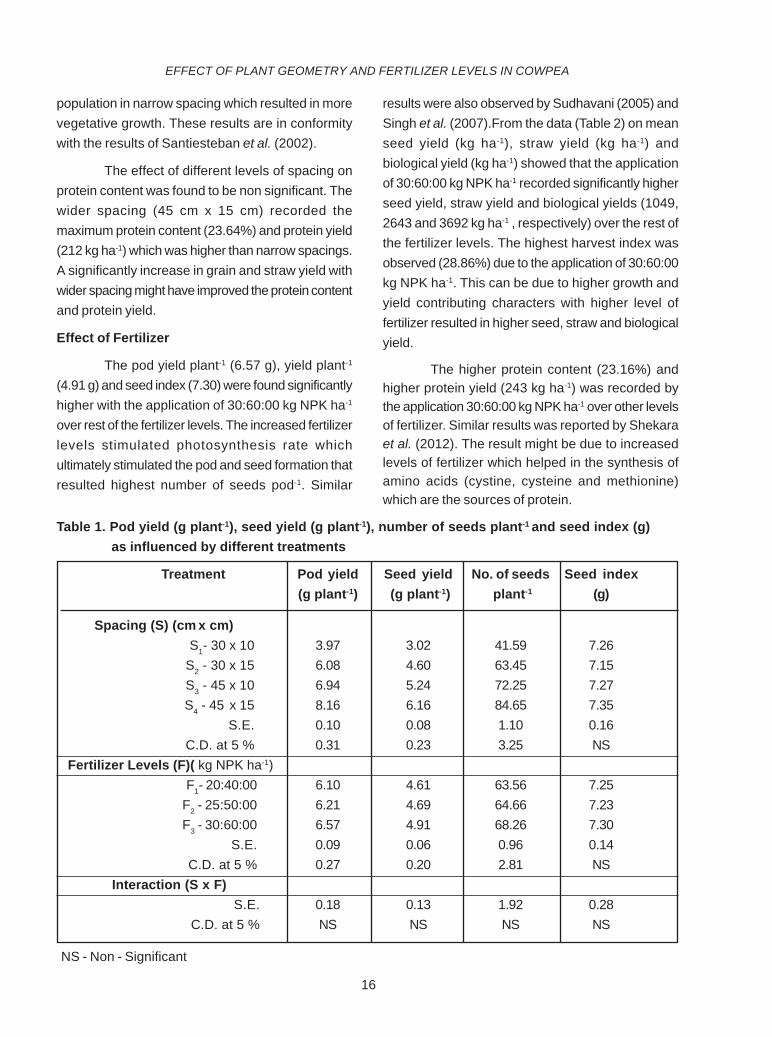
Data from Table 1 showed that the widerspacing (45 cm x 15 cm) recorded significantly higherpod yield plant-1 (8.16 g), higher mean seed yield(6.16 g plant-1) and highest seed index (7.35 g)followed by the spacing 45 cm x 10 cm (6.94 g, 5.24g and 7.27, respectively) which was higher thannarrow spacing. It might be due to wider spacingwhich reduced crowding of cowpea and got moresunlight, more nutrients resulted in higherreproductive growth of cowpea. These results are inconformity with the results of Patel et al. (2008).
Data on mean seed yield (kg ha-1), biologicalyield (kg ha-1), harvest index (HI) as influenced bydifferent levels of spacing was found significant withthe wider spacing of 45 cm x 10 cm and recordedsignificantly higher seed yield (1143 kg ha-1),biological yield (3780 kg ha-1) and harvest index(30.23 %) was followed by the closer spacing 30 x15 cm (998 kg ha-1, 3410 kg ha-1 and 29.21 %,respectively. This variation in seed yield, biological(kg ha-1) might be due to different spacings whichhad different plant population ha-1. Similar results werereported by Singh et al. (2012).
The straw yield (kg ha-1) as influenced bydifferent levels of spacing was found to be significant.The narrow spacing of 30 cm x 10 cm (3,33,333plants ha-1) recorded maximum straw yield (2733 kgha-1) which was found significantly superior to otherspacings and was at par with spacing 45 cm x 10cm (2,22,222 plants ha-1) and recorded straw yieldof 2637 kg ha-1. This might be due to higher plant
JAGADALE et al.
16
population in narrow spacing which resulted in morevegetative growth. These results are in conformitywith the results of Santiesteban et al. (2002).
The effect of different levels of spacing onprotein content was found to be non significant. Thewider spacing (45 cm x 15 cm) recorded themaximum protein content (23.64%) and protein yield(212 kg ha-1) which was higher than narrow spacings.A significantly increase in grain and straw yield withwider spacing might have improved the protein contentand protein yield.
Effect of Fertilizer
The pod yield plant-1 (6.57 g), yield plant-1
(4.91 g) and seed index (7.30) were found significantlyhigher with the application of 30:60:00 kg NPK ha-1
over rest of the fertilizer levels. The increased fertilizerlevels stimulated photosynthesis rate whichultimately stimulated the pod and seed formation thatresulted highest number of seeds pod-1. Similar
results were also observed by Sudhavani (2005) andSingh et al. (2007).From the data (Table 2) on meanseed yield (kg ha-1), straw yield (kg ha-1) andbiological yield (kg ha-1) showed that the applicationof 30:60:00 kg NPK ha-1 recorded significantly higherseed yield, straw yield and biological yields (1049,2643 and 3692 kg ha-1 , respectively) over the rest ofthe fertilizer levels. The highest harvest index wasobserved (28.86%) due to the application of 30:60:00kg NPK ha-1. This can be due to higher growth andyield contributing characters with higher level offertilizer resulted in higher seed, straw and biologicalyield.
The higher protein content (23.16%) andhigher protein yield (243 kg ha-1) was recorded bythe application 30:60:00 kg NPK ha-1 over other levelsof fertilizer. Similar results was reported by Shekaraet al. (2012). The result might be due to increasedlevels of fertilizer which helped in the synthesis ofamino acids (cystine, cysteine and methionine)which are the sources of protein.
Table 1. Pod yield (g plant-1), seed yield (g plant-1), number of seeds plant-1 and seed index (g) as influenced by different treatments
Treatment Pod yield Seed yield No. of seeds Seed index(g plant-1) (g plant-1) plant-1 (g)
Spacing (S) (cm x cm)S1- 30 x 10 3.97 3.02 41.59 7.26
S2 - 30 x 15 6.08 4.60 63.45 7.15S3 - 45 x 10 6.94 5.24 72.25 7.27S4 - 45 x 15 8.16 6.16 84.65 7.35
S.E. 0.10 0.08 1.10 0.16C.D. at 5 % 0.31 0.23 3.25 NS
Fertilizer Levels (F)( kg NPK ha-1)F1- 20:40:00 6.10 4.61 63.56 7.25
F2 - 25:50:00 6.21 4.69 64.66 7.23F3 - 30:60:00 6.57 4.91 68.26 7.30
S.E. 0.09 0.06 0.96 0.14C.D. at 5 % 0.27 0.20 2.81 NS
Interaction (S x F)S.E. 0.18 0.13 1.92 0.28
C.D. at 5 % NS NS NS NS
NS - Non - Significant
EFFECT OF PLANT GEOMETRY AND FERTILIZER LEVELS IN COWPEA

17
Table 2. Seed yield (kg ha-1), straw yield (kg ha-1), biological yield (kg ha-1) and harvest index (%)as influenced by different treatments
Treatment Seed Straw Biological Harvest yield (kg ha-1) yield (kg ha-1) yield (kg ha-1) index (%)
Spacing (S) (cm x cm)S1- 30 x 10 968 2733 3701 26.15
S2 - 30 x 15 998 2418 3416 29.21S3 - 45 x 10 1143 2637 3780 30.23S4 - 45 x 15 897 2367 3264 27.48
S.E. 17 70 69 -C.D. at 5 % 52 207 203 -
Fertilizer levels (F)(kg NPK ha-1)
F1- 20:40:00 967 2613 3351 27.01F2 - 25:50:00 987 2589 3577 27.60F3 - 30:60:00 1049 2643 3692 28.86
S.E. 15 61 60 -C.D. at 5 % 45 179 176 -
Interaction (S x F)
S.E. 31 122 120 -C.D. at 5 % NS NS NS -
Table 3. Protein content (%) and protein yield (kg ha-1) as influenced by different treatments
Treatment Protein content (%) Protein yield (kg ha-1)
Spacing (S) (cm x cm)S1- 30 x 10 22.80 220
S2 – 30 x 15 23.12 230S3 - 45 x 10 S4 - 45 x 15 23.2123.64 265212
S.E. 0.62 9.1CD at 5 % NS 26.3
Fertilizer levels (F) (kg NPK ha-1)F1- 20:40:00 22.82 220
F2 - 25:50:00 23.14 228F3 - 30:60:00 23.16 243
S.E. 0.51 14.3CD at 5 % NS 41
Interaction (S x F)S.E. 0.98 15
CD at 5% NS NS
NS - Non - Significant
NS - Non - Significant
JAGADALE et al.
18
CONCLUSION
Cowpea crop grown in kharif seasonproduced significantly higher yield attributes, seedyield and protein content with wider spacing of 45cm x 10 cm and fertilizer level i.e. application of30:60:00 kg NPK ha-1.
REFERENCES
FAO. 2012. FAO Bulletin of Statistics. Division ofEconomics and Social DevelopmentDepartment. 2: 54.
Kumar, R. K and Sudhavani, V. 2004. Effect of plantdensities and phosphorus levels on thegrowth and yield of vegetable cowpea.M.Sc Thesis submitted to Dr.Y.S.R.Horticultural University, Venkataraman-nagudem, Andhra Pradesh.
Naim, A.M.E and Jabereldar, A.A. 2010. Effect ofplant density and cultivar on growth andyield of cowpea (Vigna unguiculata (L.)Walp) Australian Journal of Basic andApplied Sciences. 4(8): 3148-3153.
Patel, B.V., Parmar B.R., Parmar S.B and Patel S.R.2008. Effect of different spacing andvarieties on yield parameters of cowpea(Vigna unguiculata L. Walp). Asian Journalof Horticulture. (6)1: 56-59.
Santiesteban, S.R., Zomora, R.A., Gomez, P.E.,Verdecia, P.P., Hernandez, G.L andZamora, Z.W. 2002. Effect of sowingdensity on IITA Precoz (Vigna unguiculata(L.) Walp) in two seasons of the year.Alimentaria. 39(32): 45-48.
Shaw, M. 2007. Most protein rich vegetarianfoods.Smarter Fitter Blog. Retrieved fromwebsite (http:/smarterfitter.com/ blog/2007on 28.1.2017) on 01.2.2017.
Shekara, B.G., Sowmyalatha, B.S and Kumar, C.B.2012. Effect of phosphorus levels on forageyield of fodder cowpea. AICRP on foragecrops, Mandya, Karnataka. pp.23-26.
Singh A.K., Bhatt, B.P., Sundaram, P.K., Kumar, S.,Bahrati, R.C., Chandra, N and Rai, M.2012. Study of site specific nutrientsmanagement of cowpea seed productionand their effect on soil nutrient status.Journal of Agricultural Science. 4(10):192.
Singh, A.K., Tripathi, P.N and Singh, R. 2007. Effectof Rhizobium inoculation, nitrogen andphosphorus level on growth, yield andquality of kharif cowpea. Crop Research.33 (1, 2 & 3):71-77.
EFFECT OF PLANT GEOMETRY AND FERTILIZER LEVELS IN COWPEA
19
INTRODUCTION
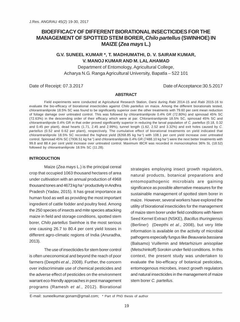
Maize (Zea mays L.) is the principal cerealcrop that occupied 1063 thousand hectares of areaunder cultivation with an annual production of 4968thousand tones and 4673 kg ha-1 productivity in AndhraPradesh (Yadav, 2015). It has great importance ashuman food as well as providing the most importantingredient of cattle fodder and poultry feed. Amongthe 250 species of insects and mite species attackingmaize in field and storage conditions, spotted stemborer, Chilo partellus Swinhoe is the most seriousone causing 26.7 to 80.4 per cent yield losses indifferent agro-climatic regions of India (Anuradha,2013).
The use of insecticides for stem borer controlis often uneconomical and beyond the reach of poorfarmers (Deepthi et al., 2008). Further, the concernover indiscriminate use of chemical pesticides andthe adverse effect of pesticides on the environmentwarrant eco-friendly approaches in pest managementprograms (Ramesh et al., 2012). Biorational
BIOEFFICACY OF DIFFERENT BIORATIONAL INSECTICIDES FOR THEMANAGEMENT OF SPOTTED STEM BORER, Chilo partellus (SWINHOE) IN
MAIZE (Zea mays L.)
G.V. SUNEEL KUMAR *, T. MADHUMATHI, D. V. SAIRAM KUMAR,V. MANOJ KUMAR AND M. LAL AHAMAD
Department of Entomology, Agricultural College,Acharya N.G. Ranga Agricultural University, Bapatla – 522 101
Date of Receipt: 07.3.2017 Date of Acceptance:30.5.2017
ABSTRACTField experiments were conducted at Agricultural Research Station, Darsi during Rabi 2014-15 and Rabi 2015-16 to
evaluate the bio-efficacy of biorational insecticides against Chilo partellus on maize. Among the different biorationals tested,chlorantraniliprole 18.5% SC was found to be significantly superior over the other treatments with 79.60 per cent mean reductionof foliage damage over untreated control. This was followed by chlorantraniliprole 0.4% GR (72.80%) and spinosad 45% SC(72.63%) in the descending order of their efficacy which were at par. Chlorantraniliprole 18.5% SC, spinosad 45% SC andchlorantraniliprole 0.4% GR in that order proved significantly superior in reducing the larval population of C. partellus (0.18, 0.32and 0.45 per plant), dead hearts (1.71, 2.45 and 2.99%), tunnel length (1.62, 2.52 and 3.32%) and exit holes caused by C.partellus (0.52 and 0.62 per plant), respectively. The cumulative effect of biorational treatments on yield indicated thatchlorantraniliprole 18.5% SC recorded the highest yield (8268.85 kg ha-1) with 108.1 per cent yield increase over untreatedcontrol. Spinosad 45% SC (7936.51 kg ha-1) and chlorantraniliprole 0.4% GR (7488.10 kg ha-1) were the next better treatments with99.8 and 88.4 per cent yield increase over untreated control. Maximum IBCR was recorded in monocrotophos 36% SL (18.52)followed by chlorantraniliprole 18.5% SC (11.28).
J.Res. ANGRAU 45(2) 19-30, 2017
E-mail: [email protected]; * Part of PhD thesis of author
strategies employing insect growth regulators,natural products, botanical preparations andentomopathogenic microbials are gainingsignificance as possible alternative measures for thesustainable management of spotted stem borer inmaize. However, several workers have explored theutility of biorational insecticides for the managementof maize stem borer under field conditions with NeemSeed Kernel Extract (NSKE), Bacillus thuringiensis(Berliner) (Deepthi et al., 2008), but very littleinformation is available on the activity of microbialpathogens especially fungus like Beauvaria bassiana(Balsamo) Vuillemin and Metarhizium anisopliae(Metschinkoff) Sorokin under field conditions. In thiscontext, the present study was undertaken toevaluate the bio-efficacy of botanical pesticides,entomogenous microbes, insect growth regulatorsand natural insecticides in the management of maizestem borer C. partellus.
20
Dos
e h
a-1
Tabl
e 1.
Fol
iage
dam
age
of m
aize
by
C. p
arte
llus
as in
fluen
ced
by th
e ap
plic
atio
n of
bio
ratio
nal i
nsec
ticid
es
dur
ing
Rab
i 201
4-15
and
201
5-16
(Poo
led
data
)
T 1A
zadi
rach
tin (
10,0
00 p
pm)
1000
ml
21.7
034
.50
36.4
040
.42
38.7
139
.88
41.0
438
.49
(35.
73)b
(37.
07)ef
(39.
20)de
(38.
47)bc
(39.
17)cd
e(3
9.86
)c(3
8.36
)de
T 2B
eauv
eria
bas
sian
a10
8 sp
ores
20.8
737
.64
27.2
427
.75
20.5
230
.47
30.4
429
.01
(37.
79)b
(31.
33)f
(31.
60)e
(26.
86)cd
(33.
39)de
(33.
25)cd
(32.
53)e
T 3M
etar
hizi
um a
niso
plia
e10
8 sp
ores
17.8
534
.35
28.7
147
.16
18.2
022
.18
15.9
727
.76
(34.
64)b
(32.
23)f
(43.
37)cd
(24.
30)d
(27.
26)e
(22.
82)d
(31.
79)e
T 4B
acill
us t
hurin
gien
sis
1 kg
18.4
468
.18
55.9
759
.30
52.1
358
.05
51.3
257
.49
(Hal
t 5%
WP
)(5
6.12
)a(4
8.45
)cd(5
0.54
)abc
(46.
32)b
(49.
83)bc
(45.
99)bc
(49.
37)c
T 5N
oval
uron
10%
EC
500
ml
18.9
844
.93
45.6
549
.15
44.6
542
.18
46.0
645
.44
(42.
06)b
(42.
51)de
(44.
53)cd
(41.
94)b
(40.
32)cd
(42.
74)c
(42.
37)d
T 6Sp
inos
ad 4
5% S
C15
0 m
l15
.90
70.1
873
.75
62.4
881
.11
77.0
971
.17
2.63
(56.
96)a
(59.
48)ab
(52.
37)ab
c(6
4.48
)a(6
1.99
)ab(5
7.78
)ab(5
8.57
)ab
T 7C
hlor
antra
nilip
role
18
.5%
SC
150
ml
15.9
178
.31
80.2
872
.77
83.0
782
.13
1.03
9.60
(62.
30)a
(63.
69)a
(58.
62)a
(65.
80)a
(65.
50)a
8(64
.72)
a(6
3.22
)a
T 8C
hlor
antra
nilip
role
0.4
% G
R10
kg
20.0
071
.49
73.3
970
.00
75.8
774
.16
71.9
22.
80(5
7.93
)a(5
9.07
)ab(5
6.86
)ab(6
1.72
)a(5
9.81
)ab(5
8.19
)ab(5
8.75
)ab
T 9C
arbo
fura
n 3G
10 k
g19
.21
68.2
465
.39
61.8
175
.32
70.8
568
.55
8.36
(55.
80)a
(54.
00)bc
(51.
88)ab
c(6
0.31
)a(5
7.51
)ab(5
5.96
)ab(5
5.80
)bc
T 10M
onoc
roto
phos
36%
SL
800
ml
20.7
073
.28
74.1
655
.03
75.2
368
.25
70.8
669
.47
(58.
91)a
(59.
53)ab
(47.
98)bc
d(6
0.52
)a(5
5.75
)ab(5
7.40
)ab(5
6.49
)b
T 11U
ntre
ated
con
trol
—20
.50
——
——
——
—SE
m±
1.49
4.21
2.05
3.13
4.59
4.30
4.33
2.25
CD
@ 5
%NS
12.4
36.
049.
2413
.54
12.6
812
.79
6.64
CV (%
)9.
9616
.10
8.01
12.5
117
.81
16.7
017
.26
8.79
Valu
es in
par
enth
eses
are
arc
sin
e tra
nsfo
rmed
val
ues
DAT
– D
ays
afte
r tre
atm
ent,
NS
: Non
Sig
nific
ant,
PTC
– P
re T
reat
men
t Cou
ntB
t – B
acill
us th
urin
gien
sis
Ser
ovar
Kur
stak
i H 3
a, 3
b, 3
c; 5
% W
P, H
alt,
5X10
7 sp
ore/
mg,
mak
e -
Bio
stad
tIn
a c
olum
n m
eans
follo
wed
by
sam
e al
phab
et d
o no
t diff
er s
igni
fican
tly b
y C
D (
P=0
.05)
T. No.
Inse
ctic
ide
% F
olia
ge d
amag
e re
duct
ion
over
con
trol
Firs
t app
licat
ion
Seco
nd a
pplic
atio
n
PTC
7 D
AT14
DAT
21 D
AT7
DAT
Pool
edm
ean
14 D
AT21
DAT
SUNEEL KUMAR et al.

21
MATERIAL AND METHODS
Field experiments were laid out in aRandomized Block Design (RBD) at AgriculturalResearch Station, Darsi with eleven treatments andreplicated thrice including untreated control toevaluate the bio-efficacy of biorational pesticidesagainst C. partellus on maize. The size of each plotwas 16.8 m2 with seven rows and 20 plants per row.The popular maize hybrid 30V92 was selected forthe experiment and was sown during Rabi season of2014-15 and 2015-16 with 0.6 m x 0.2 m spacingbetween row to row and plant to plant. For uniforminfestation in trial plots, egg masses of C. partellusat black-head stage obtained from laboratory cultureswere taken to experimental site and 10 egg masseswere pinned randomly on whorl leaves of 15-20 dayold plants in the central four rows in each treatmentplot. A total of 330 egg masses were placed in theentire experimental plot.
The biopesticides viz., Beauveria bassianaVuillemin and Metarhizium anisopliae Metchnikoffwere obtained from Department of Microbiology, PostHarvest Technology Centre, Bapatla. Bacillusthuriengensis Serovar Kurstaki H 3a, 3b, 3c; (Halt5% WP, 5X10⁷ spore/mg) manufactured by Biostadtwas obtained locally. The standard checks used weremonocrotophos 36 SL and carbofuran 3G. All thetreatments were imposed two times, i.e., 25th and47th day after emergence of the crop.
Observations on stem borer damage wasrecorded as fresh leaf damage with shot holes inrandomly selected 10 plants in each replication ofthe treatment leaving border rows to avoid bordereffect. The observations were recorded one day beforetreatment as pre-treatment count and at 7, 14 and21 days after each spray as post-treatment countsand per cent infestation / damage was worked out.Observations recorded on 21st day after first sprayserved as the pre-treatment count for the secondspray. For the extent of infestation, dead heartswere also used as criteria for infested plants. The
individual data of dead hearts at 30 (after first spray)and 50 (after second spray) days after treatment wastaken which was then converted into total per centdead heart damage on the basis of total plant standand mean per cent damage for the season. At thetime of harvest, the total number of larvae per 10plants was recorded by destructive sampling. Theselected plants were uprooted and number of exitholes was recorded. Next, the stems were splitopened to count the number of larvae or pupae of C.partellus and the tunnelling length was recorded. Percent stem tunnelling was calculated on the basis oftotal tunneled length divided by plant height of affectedplant. Average per cent stem tunneling per plotwas calculated by dividing average tunnel lengthby average length of plants taken for tunnellingobservation. At 7, 14 and 21 DAE, observation fornatural enemies was also made in the treatmentplots of each replication.
The net plots were harvested, dried, shelledand cleaned replication wise separately excludingborder rows and yield per plot was expressed as kgper plot, based on which yield per hectare wascalculated. The cost economics of each treatmentwas calculated to find out the most economic methodof stem borer management in maize. Benefit-costratio was calculated by dividing the extra benefitattained from enhanced yield by the extra costincurred for each treatment. The percentage valuesand mean population data were duly transformed intothe corresponding angular and square roottransformed values and were subjected to statisticalanalysis using the analysis of variance for randomizedblock design. Critical difference values werecalculated at 5% probability level and the treatmentmean values were compared using Duncan’s MultipleRange Test.
RESULTS AND DISCUSSION
The overall cumulative efficacy of all theobservations made at 7, 14 and 21 days after eachspray of different biorational insecticides during two
BIOEFFICACY OF BIORATIONAL INSECTICIDES IN SPOTTED STEM BORER MANAGEMENT

22
Dos
eha
-1
Tabl
e 2.
Effe
ct o
f bio
ratio
nal i
nsec
ticid
es u
se o
n th
e da
mag
e ca
used
by
C. p
arte
llus
in m
aize
dur
ing
Rab
i 201
4-15
and
201
5-16
T 1A
zadi
rach
tin (
10,0
00 p
pm)
1000
ml
8.85
9.33
9.09
6.87
11.5
09.
197.
8610
.42
9.14
(17.
28)b
(17.
77)bc
d(1
7.53
)bc(1
5.15
)b(1
9.83
)b(1
7.64
)b(1
6.25
)b(1
8.83
)bc(1
7.59
)bc
T 2B
eauv
eria
bas
sian
a10
85.
089.
977.
524.
7010
.89
7.80
4.89
10.4
37.
66sp
ores
(12.
95)cd
(18.
27)bc
(15.
91)bc
d(1
2.39
)cd(1
9.20
)b(1
6.13
)b(1
2.67
)cd(1
8.85
)bc(1
6.06
)c
T 3M
etar
hizi
um a
niso
plia
e10
87.
7812
.68
10.2
36.
5612
.09
9.32
7.17
12.3
99.
78sp
ores
(16.
21)bc
(20.
68)ab
(18.
61)b
(14.
84)bc
(20.
35)b
(17.
78)b
(15.
54)bc
(20.
55)b
(18.
21)b
T 4B
acill
us t
hurin
gien
sis
2.64
9.09
5.86
2.21
7.61
4.91
2.42
8.35
5.39
(Hal
t 5%
WP
)1
kg(9
.20)
e(1
7.55
)bcd
(14.
01)de
(8.4
1)ef
(16.
02)c
(12.
80)cd
(8.8
1)ef
(16.
80)c
(13.
42)de
T 5N
oval
uron
10%
EC
500
ml
3.85
9.39
6.62
2.66
7.38
5.02
3.26
8.38
5.82
(11.
12)de
(17.
79)bc
d(1
4.83
)cde
(9.3
4)ef
(15.
74)c
(12.
94)c
(10.
28)de
f(1
6.82
)c(1
3.93
)d
T 6Sp
inos
ad 4
5% S
C15
0 m
l1.
923.
622.
771.
622.
652.
141.
773.
132.
45(7
.86)
ef(1
0.88
)ef(9
.49)
gh(7
.22)
fg(9
.36)
f(8
.37)
fg(7
.54)
fg(1
0.15
)fg(8
.95)
gh
T 7C
hlor
antr
anili
prol
e0.
962.
401.
680.
872.
611.
740.
912.
511.
7118
.5%
SC
150
ml
(4.6
0)f
(8.5
4)f
(7.0
2)h
(5.2
8)g
(9.2
6)f
(7.5
8)g
(5.2
7)g
(9.0
6)g
(7.4
5)h
T 8C
hlor
antr
anili
prol
e1.
924.
073.
002.
283.
702.
992.
103.
892.
990.
4% G
R10
kg
(7.8
7)ef
(11.
39)ef
(9.8
7)fg
h(8
.53)
ef(1
1.10
)ef(9
.94)
ef(8
.23)
ef(1
1.30
)ef(9
.91)
fg
T 9C
arbo
fura
n 3G
10 k
g3.
596.
515.
053.
254.
063.
653.
425.
284.
35(1
0.89
)de(1
4.72
)cde
(12.
95)de
f(1
0.37
)de(1
1.62
)de(1
1.02
)de(1
0.64
)de(1
3.27
)de(1
2.02
)de
T 10M
onoc
roto
phos
36%
SL
800
ml
2.93
5.90
4.41
2.70
5.17
3.94
2.81
5.54
4.18
(9.6
7)de
(13.
93)de
(11.
98)ef
g(9
.23)
ef(1
3.13
)d(1
1.38
)cde
(9.4
6)ef
(13.
54)d
(11.
69)ef
T 11U
ntre
ated
con
trol
—13
.19
16.3
214
.76
12.3
115
.96
14.1
412
.75
16.1
44.
45(2
1.30
)a(2
3.82
)a(2
2.60
)a(2
0.54
)a(2
3.55
)a(2
2.09
)a(2
0.93
)a(2
3.70
)a1(
22.3
5)a
SEm
±1.
241.
421.
080.
930.
640.
620.
990.
730.
70C
D @
5 %
3.67
4.19
3.19
2.75
1.90
1.82
2.92
2.15
2.08
CV (%
)18
.34
15.4
013
.31
14.6
77.
257.
9415
.02
8.00
8.83
Valu
es in
par
enth
eses
are
arc
sin
e tra
nsfo
rmed
val
ues
;
D
AE
– D
ays
afte
r em
erge
nce
Bt –
Bac
illus
thur
ingi
ensi
s S
erov
ar K
urst
aki H
3a,
3b,
3c;
5%
WP,
Hal
t, 5X
107 sp
ore/
mg,
mak
e -
Bio
stad
tIn
a c
olum
n m
eans
follo
wed
by
sam
e al
phab
et d
o no
t diff
er s
igni
fican
tly b
y C
D (
P=0
.05)
T. No.
Inse
ctic
ide
Per
cent
dea
d he
arts
Rab
i 20
14-1
5Po
oled
30
DA
E50
DA
EM
ean
Rab
i 20
15-1
6
30
DA
E50
DA
EM
ean
30
DA
E50
DA
EM
ean
SUNEEL KUMAR et al.
23
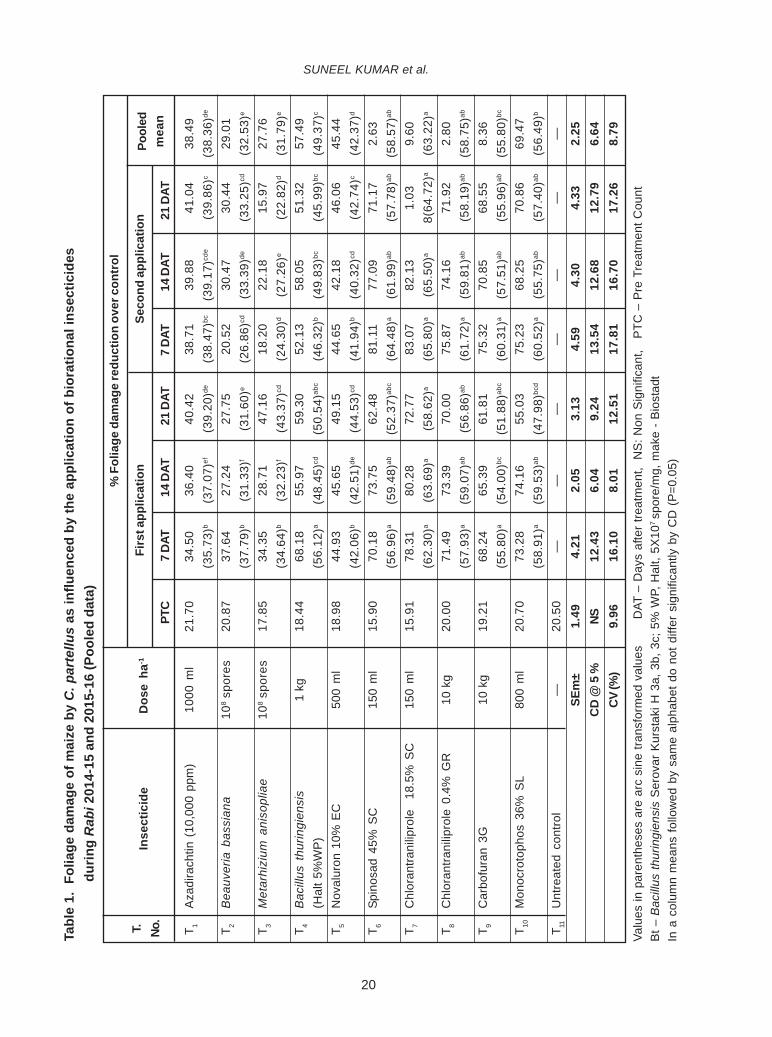
successive seasons viz., Rabi 2014-15 and Rabi2015-16 on stem borer foliage damage reduction overcontrol was presented in Table 1. The results showedthat chlorantraniliprole 18.5% SC was found to besignificantly superior at all the intervals of spraysequence over the other treatments and recorded79.60 per cent mean reduction of foliage damageover untreated control. This was followed bychlorantraniliprole 0.4% GR (72.80%) and spinosad45% SC (72.63%) in the descending order of theirefficacy which were at par. The higher per cent ofdamage reduction may be due to the application ofthese chemicals at the initiation of infestation makesborers unable to overcome the impact of early exhaustand to make a heavy population build up. The resultspertaining to chlorantraniliprole are in agreement withAnuradha (2013) who reported 1.27 to 2.96 per centinfestation in maize during Kharif and 1.06 to 5.60during Rabi in four dosages of coragen. The besttreatment in reducing leaf injury (3.43 & 4.23 %) byC. partellus was recorded with chlorantriniliprole 18.5SC during 2012 and 2013 (Ravinder and Jindal, 2015).Significantly less infestation of C. partellus (4.5% at25 DAS and 7.42% at 40 DAS) in maize wasobserved with the treatment of chlorantraniliprole(Kumar et al., 2015). Yadav (2015) also confirmedthe superiority of chlorantriniliprole 20 SC in reducingthe borer infestation in maize based on leaf injuryrating observed at 25 days after infestation at AICRPcenters working on maize during Kharif, 2014. Thepresent results about spinosad are in close line withSohail et al. (2002) who showed the efficacy ofspinosad to reduce C. partellus infestation from10.72% to almost negligible level (0.74%). MunirAhmad et al. (2010) reported the effectiveness ofspinosad 240 EC @ 40 ml acre-1 with reduced borerinfestation of 1.2 per cent when compared to thecontrol (38.1%). Similar findings were recorded withRamesh et al. (2012) who reported that the maizestem borer infestation levels were significantly lowin spinosad (1.67%). Similar trend was observed withShahzad et al. (2010) on the superiority of spinosadagainst stem borer of maize.
In the present study, monocrotophos 36%SL was found to be next best with 69.47 per centreduction in foliage damage and was found to be onpar with carbofuran 3G (68.36%) and B. thuringiensis5% WP (57.49%). Similar results were also recordedby Saeed et al. (2006) who reported that stem borerswere significantly controlled by spraying withmonocrotophos. The efficacy of monocrotophos wasalso supported by Ramesh et al. (2012) who reportedthat bioefficacy of monocrotophos (0.00 to 3.33 %)was found to be on par with that of spinosad (1.67 to6.7%). The superiority of carbofuran against maizestem borer is in close conformity with theobservations of Radha et al. (2006) who reportedfoliar damage per cent of 6.53 and 83.60 per centreduction in larval population over untreated controlin maize with carbofuran. Similar trend was observedwith results of Nagarjuna (2005). Similarly, Singhand Sharma (2009) concluded that application ofcarbofuron 3G (15 kg ha-1) was found to be effectivein controlling of C. partellus with 8.93 and 7.53 percent plant infestation during Kharif 2006 and 2007,respectively. Further, Saleem et al. (2014) andKulkarni et al. (2015) reported that whorl applicationof carbofuran 3G @ 7.5 kg ha-1 proved to be the bestbased on leaf injury, pest infestation, stem tunnelingand grain yield which performed highly effective andeconomical in reducing the stem borer damage inmaize. Jyothi et al. (2016) also reported thesuperiority of carbofuran with lowest foliage damageof 11.7 per cent and 84.28 per cent mean reductionof stem borer larval population in treated maize plots.In addition to this, the efficacy of granules may bedue to the fact that young larvae before gaining entryin to the stem feed in the leaf whorl and get exposedto insecticides placed in the leaf whorls leading tothe better efficacy of the insecticide.
In the present study, the biopesticide B.thuringiensis was also found to provide significantreduction in the stem borer. The present studies arein close agreement with Kandalkar and Men (2006)who reported that Bt spray was found to be the best
BIOEFFICACY OF BIORATIONAL INSECTICIDES IN SPOTTED STEM BORER MANAGEMENT

24
Dos
eha
-1
Tabl
e 3.
Effe
ct o
f bio
ratio
nal i
nsec
ticid
es u
se o
n th
e C
. par
tellu
s la
rval
den
sity
, exi
t hol
es a
nd
s
tem
tunn
elin
g at
har
vest
in m
aize
dur
ing
Rab
i 201
4-15
and
201
5-16
T 1A
zadi
rach
tin (
10,0
00 p
pm)
1000
ml
1.47
1.07
1.27
1.43
1.00
1.22
9.70
6.43
8.07
(1.2
1)a
(1.0
2)bc
(1.1
3)b
(1.2
0)bc
(1.0
0)b
(1.1
0)b
(18.
11)bc
(14.
64)ab
c(1
6.49
)b
T 2B
eauv
eria
bas
sian
a10
8 sp
ores
1.40
1.23
1.32
1.70
1.07
1.38
12.2
76.
109.
18(1
.18)
a(1
.10)
b(1
.14)
b(1
.30)
b(1
.03)
b(1
.17)
b(2
0.47
)b(1
4.11
)bcd
(17.
58)b
T 3M
etar
hizi
um a
niso
plia
e10
8 sp
ores
1.40
1.20
1.30
1.37
1.10
1.23
12.3
76.
709.
53(1
.18)
a(1
.08)
b(1
.14)
b(1
.17)
c(1
.04)
b(1
.11)
b(2
0.60
)b(1
4.86
)ab(1
7.98
)b
T 4B
acill
us t
hurin
gien
sis
1 kg
0.53
0.90
0.72
0.93
1.00
0.97
6.93
3.57
5.25
(Hal
t 5%
WP
)(0
.73)
bc(0
.93)
bc(0
.84)
c(0
.97)
d(0
.99)
b(0
.98)
c(1
5.16
)cd(1
0.83
)cde
(13.
23)c
T 5N
oval
uron
10%
EC
500
ml
0.73
0.77
0.75
1.00
0.80
0.90
7.47
3.53
5.50
(0.8
5)b
(0.8
7)cd
(0.8
7)c
(0.9
9)d
(0.8
9)bc
(0.9
4)cd
(15.
85)cd
(10.
64)de
(13.
51)c
T 6Sp
inos
ad 4
5% S
C15
0 m
l0.
300.
330.
320.
870.
370.
624.
070.
972.
52(0
.54)
cd(0
.58)
ef(0
.56)
e(0
.93)
de(0
.60)
d(0
.78)
ef(1
1.52
)ef(5
.45)
f(9
.07)
ef
T 7C
hlor
antr
anili
prol
e0.
200.
170.
180.
700.
330.
522.
300.
931.
6218
.5%
SC
150
ml
(0.4
4)d
(0.4
1)f
(0.4
2)f
(0.8
3)e
(0.5
8)d
(0.7
2)f
(8.5
9)f
(5.4
3)f
(7.1
7)f
T 8Ch
lora
ntra
nilip
role
0.4
% G
R10
kg
0.50
0.40
0.45
0.87
0.37
0.62
5.37
1.27
3.32
(0.7
1)bc
(0.6
2)e
(0.6
8)de
(0.9
2)de
(0.6
1)d
(0.7
8)ef
(13.
13)de
(6.1
4)f
(10.
27)de
T 9C
arbo
fura
n 3G
10 k
g0.
600.
530.
570.
870.
570.
725.
903.
234.
57(0
.76)
b(0
.72)
de(0
.75)
cd(0
.92)
de(0
.75)
cd(0
.84)
de(1
3.80
)de(1
0.35
)de(1
2.23
)cd
T 10M
onoc
roto
phos
36%
SL
800
ml
0.50
0.50
0.50
.90
0.53
0.72
5.17
2.73
3.95
(0.7
1)bc
(0.7
1)de
(0.7
0)d
0(0.
95)de
(0.7
3)cd
(0.8
4)de
(13.
11)de
(9.1
0)ef
(11.
38)cd
e
T 11U
ntre
ated
con
trol
—1.
872.
272.
072.
202.
502.
3520
.13
9.73
14.9
3(1
.36)
a(1
.50)
a(1
.44)
a(1
.49)
a(1
.57)
a(1
.53)
a(2
6.64
)a(1
8.16
)a(2
2.74
)a
SEm
±0.
060.
060.
040.
040.
080.
021.
081.
320.
87C
D @
5 %
0.19
0.19
0.13
0.13
0.18
0.10
3.17
3.89
2.58
CV (%
)13
.03
13.1
88.
477.
0512
.18
6.47
11.6
121
.02
10.9
9†
Valu
es in
par
enth
eses
are
arc
sin
e tra
nsfo
rmed
val
ues
;
*
Valu
es in
par
enth
eses
are
squ
are
root
tran
sfor
med
val
ues
Bt –
Bac
illus
thur
ingi
ensi
s S
erov
ar K
urst
aki H
3a,
3b,
3c;
5%
WP,
Hal
t, 5X
107 sp
ore/
mg,
mak
e -
Bio
stad
tIn
a c
olum
n m
eans
follo
wed
by
sam
e al
phab
et d
o no
t diff
er s
igni
fican
tly b
y C
D (
P=0
.05)
T. No.
Inse
ctic
ide
*No.
of l
arva
e p
lant
-1†
Per c
ent s
tem
tunn
elin
g
Rab
i20
14-1
5R
abi
2015
-16
Pool
edM
ean
*Exi
t hol
es p
lant
-1
Rab
i20
14-1
5R
abi
2015
-16
Pool
edM
ean
Rab
i20
14-1
5R
abi
2015
-16
Pool
edM
ean
SUNEEL KUMAR et al.

25
treatment with the least number of dead hearts, leafinjury and maximum grain yield in maize. Novaluron10% EC and azadirachtin 10000 ppm recorded lowerefficacy compared to other biorationals due to thefact that stem borer larvae had the peculiar habit oftunneling of stems. This typical behaviour might haveprotected the larvae from acquiring the slow actinginsecticide coming in contact with insect directly.However, these insecticides showed effectivenessin reducing the foliage damage (45.44% and 38.49%)when compared to untreated control. The presentresults are in agreement with Ramesh et al. (2012)who reported that novaluron (0.01%) anddiflubenzuron (0.02%) significantly inferior to otherbiorational treatments in checking the maize stemborer damage and infestation levels were on par withthat of untreated check during Kharif 2008 and 2009at Sikkim.
The entomopathogenic fungi B. bassianaand M. anisopliae were found to provide unsatisfactorycontrol of C. partellus in the present study which isin agreement with the results reported by Spruthiand Shekarappa (2007). However, few earlier reportsestablished the efficacy of these fungi against themaize stem borer under field conditions (Shekarappa,2001). Selection of potential isolates of theentomopathogenic fungi seems to be a prerequisiteto achieve a satisfactory control of C. partellus. Thetype of formulation of biocontrol agent was found tomake significant difference in their efficacy. Maniania(1993) found that application of granulatedformulation of B. bassiana was more effective thanspray application at the same concentration,probably owing to its greater persistence.
At both the intervals of observation (30 and50 DAE) treatments with chlorantraniliprole 18.5%SC, spinosad 45% SC and chlorantraniliprole 0.4%GR were found to be most effective which recordedleast per cent dead hearts. Among rest of thetreatments B. thuringiensis 5% WP (2.42%) was onpar with monocrotophos 36% SL (2.81%) at 30 DAEfollowed by novaluron 10% EC (3.26%) and carbofuran
3 G (3.42%). However, at 50 DAE carbofuran 3 G(5.28%) was found to be on par with monocrotophos36% SL (5.54%). Treatments including B.thuringiensis 5% WP (8.35%) and novaluron 10%EC (8.38%) were next in the order of efficacy. Themean values revealed the superiority of treatmentsin the order of chlorantraniliprole 18.5% SC (1.71%)> spinosad 45% SC (2.45%) > chlorantraniliprole0.4% GR (2.99%) > monocrotophos 36% SL (4.18%)> carbofuran 3 G (4.35%) > B. thuringiensis 5% WP(5.39%) > novaluron 10% EC (5.82%) > B. bassiana(7.66%) > Azadirachtin 10000 ppm (9.14%) > M.anisopliae (9.78%) which reiterated the result of twoyears of experimentation (Table 2). The results arein agreement with Anuradha (2013) who reported 0.0to 0.68 and 0.0 to 4.31 per cent dead hearts in maizeduring kharif and rabi, respectively in four dosagesof chlorantraniliprole. The best treatment in reducingdead hearts (3.16 and 3.90%) by C. partellus wasrecorded with chlorantriniliprole 18.5 SC during 2012and 2013 (Ravinder and Jindal, 2015). Similar trendwas observed by Kumar et al. (2015) who reportedthat chlorantraniliprole 18.5 SC was the best withminimum number of dead hearts (2.33 % at 25 DASand 1.66 % at 40 DAS). The results pertaining tomonocrotophos (4.18%) are in agreement with Saeedet al. (2006) who reported that stem borer of maizewas significantly controlled by monocrotophos. Theefficacy of monocrotophos was also supported byRamesh et al. (2012) who reported thatmonocrotophos (0.05%) significantly reduced thedamage of C. partellus. The present findings showedthat carbofuran is next best (4.35%) and the resultsare in agreement with Kakar et al. (2003) whorecorded 2.01 per cent dead hearts. Similar trendwas observed with Radha et al. (2006) who reportedthat carbofuran 3G @ 0.3 kg a.i. ha-1 recorded 7.8per cent dead hearts. Saleem et al. (2014) alsoreported that average dead hearts count for carbofuran3G was 3.17 per cent. Similar results were alsorecorded with Kulkarni et al. (2015) and Jyothi et al.(2016) with respect to carbofuran against maize stem
BIOEFFICACY OF BIORATIONAL INSECTICIDES IN SPOTTED STEM BORER MANAGEMENT

26
Dos
eha
-1
Tabl
e 4.
Effe
ct o
f bio
ratio
nal i
nsec
ticid
es u
se o
n yi
eld
and
cost
eco
nom
ics
for t
he c
ontr
ol o
f C. p
arte
llus
in M
aize
T 1A
zadi
rach
tin (
10,0
00 p
pm)
1000
ml
4708
.33ef
5734
.13ef
5221
.23f
1248
.02
31.4
316
224.
2130
89.0
013
135.
215.
25
T 2B
eauv
eria
bas
sian
a10
8 sp
ores
4662
.70ef
5575
.40ef
5119
.05f
1145
.83
28.8
714
895.
8331
79.0
011
716.
834.
69
T 3M
etar
hizi
um a
niso
plia
e10
8 sp
ores
4513
.89f
5039
.68fg
4776
.79f
803.
5720
.25
1044
6.43
2470
.00
7976
.43
4.23
T 4B
acill
us t
hurin
gien
sis
(Hal
t 5%
WP
)1
kg48
27.3
8de59
52.3
8ef53
89.8
8f14
16.6
735
.69
1841
6.67
1786
.00
1663
0.67
10.3
1
T 5N
oval
uron
10%
EC
500
ml
5025
.79d
7301
.59cd
6163
.69e
2190
.48
55.1
328
476.
1946
67.0
023
809.
196.
10
T 6Sp
inos
ad 4
5% S
C15
0 m
l69
44.4
4a89
28.5
7ab79
36.5
1ab39
63.2
999
.77
5152
2.82
5738
.00
4578
4.82
8.98
T 7C
hlor
antr
anili
prol
e18
.5%
SC
150
ml
7152
.78a
9384
.92a
8268
.85a
4295
.63
108.
1255
843.
2545
48.0
051
295.
2512
.28
T 8C
hlor
antr
anili
prol
e0.
4% G
R10
kg
6642
.86b
8333
.33ab
c74
88.1
0bc35
14.8
888
.44
4569
3.45
4788
.00
4090
5.45
9.54
T 9C
arbo
fura
n 3G
10 k
g59
68.2
5c79
36.5
1bcd
6952
.38cd
2979
.17
75.0
338
729.
1735
00.0
035
229.
1711
.07
T 10M
onoc
roto
phos
36%
SL
800
ml
5948
.41c
6646
.83de
6297
.62de
2324
.40
58.4
930
217.
2615
48.0
028
669.
2619
.52
T 11U
ntre
ated
con
trol
—37
20.2
4g42
26.1
9g39
73.2
1g—
——
——
—
SEm
±93
.70
447.
9322
9.86
CD
@ 5
%27
6.41
1321
.41
678.
10
CV%
2.97
11.3
46.
48
Mar
ket P
rice
of M
aize
: Rs.
13/
- per
kg;
Sta
ndar
d sp
ray
volu
me:
500
l/ha
; *La
bour
and
spr
ayer
cha
rges
incl
udin
g fo
r tw
o sp
rays
In a
col
umn
mea
ns fo
llow
ed b
y sa
me
alph
abet
do
not d
iffer
sig
nific
antly
by
CD
(P
=0.0
5)
T. No.
Inse
ctic
ide
Gra
in Y
ield
(kg
ha-1)
Rab
i20
14-1
5R
abi
2015
-16
Pool
edM
ean
Incr
emen
tal
Yiel
dove
rco
ntro
l(k
g ha
-1)
Incr
ease
inyi
eldo
ver
cont
rol
(%)
Valu
e of
incr
e-m
enta
lyi
eld
(Rs)
*Cos
t of
plan
tpr
otec
tion
(Rs
ha-1)
Net
prof
it (R
sha
-1)
Incr
em
enta
lB
:C ra
tio
SUNEEL KUMAR et al.

27
borers. Spray application of B. thuringiensis had givensatisfactory results (5.39%) in this study as indicatedby Deepthi et al. (2008) who reported that B.thuringiensis (1 g litre-1) was the most effective inreducing dead hearts damage (9.68%) due to stemborer.
The pooled mean larval population of C.partellus indicated the lowest population of 0.18larvae per plant in chlorantraniliprole 18.5% SC withmaximum population in untreated check (2.07 larvaeplant-1). The overall efficacy of the biorationaltreatments against the number of exit holes indicatedthat chlorantraniliprole 18.5% SC was superior overthe other biorational treatments and recordedminimum number of exit holes per plant (0.52)followed by spinosad 45% SC and chlorantraniliprole0.4% GR (0.62) which were on par. The next effectivetreatments are carbofuran 3G (0.87) andmonocrotophos 36% SL (0.72) which were on parwith each other. The maximum numbers of exit holeswere recorded with azadirachtin 10000 ppm (1.22),M. anisopliae (1.23) and B. bassiana (1.38) whichwere on par with each other but were significantlydifferent from control (2.35). The results are inagreement with Lucius and Oniemayin (2011) whoreported 1.00 numbers of exit holes when treatedwith carbofuron compared to control (4.00) andsimilar trend was observed with Pavani (2011) whoreported 0.80 exit holes per plant treated withcarbofuron. Jyothi et al. (2016) also found minimumnumber of exit holes caused by stem borer incarbofuran (1.92) and spinosad (3.59) treated maizeplots. Chlorantraniliprole 18.5% SC was statisticallysuperior to other treatments with mean lowesttunneling of 1.62 per cent and followed by spinosad45% SC (2.52%). Next best were chlorantraniliprole0.4% GR, monocrotophos 36% SL, carbofuran 3Gand B.thuringiensis 5% WP which recorded 3.32,3.95, 4.57 and 5.25 per cent, respectively. Maximumstem tunneling was noticed in untreated check with14.93 per cent (Table 3). The superiority ofchlorantraniliprole against maize stem borer is in
accordance with the works of earlier authors whorecorded minimum tunnel length (1.94 cm) withchlorantraniliprole (Kumar et al., 2015). The resultsare also in agreement with Lucius and Oniemayin(2011) who reported 1.0 cm tunnel length when treatedwith carbofuran compared to control (5.53cm) andthe similar trend was observed with Pavani (2011)who reported 0.35 cm tunneling with carbofuran.Jyothi et al. (2016) also recorded a tunnel length of2.73 cm in maize treated with carbofuran which wason par with flubendiamide (2.83 cm) and spinosad(4.13 cm). The results pertaining to B. thuringiensiswas in close line with Deepthi et al. (2008) whoreported 15.43 per cent tunneling when treated withB. thuringiensis compared to untreated control(22.30%).
Pooled analysis of yield data also confirmedthe superiority of all the treatments over untreatedcontrol (3973.21 kg ha-1). Superiority ofchlorantraniliprole 18.5% SC (8268.85 kg ha-1)followed by spinosad 45% SC (7936.51 kg ha-1) andchlorantraniliprole 0.4% GR (7488.10 kg ha-1) overother inputs was reiterated (Table 4). This finding wasin agreement with Ravinder and Jindal (2015) whoreported that economic returns on the basis ofmarketable grain was more in chlorantriniliprole (51.99q ha-1) in comparison to control (40.44 q ha-1) andbiological control plots (46.75 q ha-1). This is also inagreement with earlier report of Kumar et al. (2015)who obtained maximum grain yield of 73.33 q ha-1
with chlorantraniliprole. The findings on spinosadcorroborate with the results of Ramesh et al. (2012)who reported that the highest yield was recordedwith spinosad (2365.50 kg ha-1) compared to control(1792.90 kg ha-1). Shahzad et al. (2010) reportedthat spinosad has recorded a grain yield of 5289 kgha-1 followed by and carbofuran (5215 kg ha-1).
The next best was carbofuran 3G (6952.38kg ha-1) with 75 per cent increase over control whichwas followed by monocrotophos 36% SL (6297.62kg ha-1, 58.5% increase over control) and novaluron
BIOEFFICACY OF BIORATIONAL INSECTICIDES IN SPOTTED STEM BORER MANAGEMENT

28
10% EC (6163.69 kg ha-1, 55% increase over control).This is in accordance with Kakar et al. (2003) whorecorded highest maize grain yield of 4952.33 kgha-1 with carbofuran. Singh and Sharma (2009)recorded higher grain yield of maize 54.97 and 51.97(q ha-1) and Jyothi (2016) recorded 35.59 q ha-1 ofmaize yield (90% yield increase over untreatedcontrol) with carbofuran as compared to rest of thetreatments also endorses the present findings oncarbofuran efficacy. Whereas, Ramesh et al. (2012)reported the increase in maize grain yield overuntreated check was 38.66 per cent formonocrotophos.
Rest of the treatments in the decreasingorder of yield were B. thuringiensis (5389.88 kg ha-1
and 36% increase over control), azadirachtin 10000ppm (5221.23 kg ha-1 and 31.43% increase overcontrol), B. bassiana (5119.05 kg ha-1 and 29%increase over control) and M. anisopliae (4776.79kg ha-1, 21% increase over control) and did not varysignificantly with each other. Earlier reports bySharma and Odak (1996) indicated B. thuringiensisapplied alone provided an increase in yield of 36 percent in maize over the untreated check. The presentstudies are also in close agreement with Bhanukiranand Panwar (2005) who reported that Bt kurstaki(17.07 q ha-1) and Neemazal – F (5.73 q ha-1) as thenext best treatments after endosulfan with respectto yield. While the inferiority of entomopathogenicfungi B. bassiana and M. anisopliae in terms of maizegrain yield confirms the earlier report of Ramesh etal. (2012). The report by Deepthi et al. (2008) revealedper cent yield increase over untreated control was23.86% for M. anisopliae followed by B. thuringiensis(23.47%) also support present findings.
The cost of intervention of different biorationaltreatments ranged from zero in untreated control toRs.5738/- per ha in spinosad 45% SC treated plots.Among the biorational treatments maximum IBCRwas recorded in chlorantraniliprole 18.5% SC (12.28)which was next best to standard chemical check,
monocrotophos 36% SL (19.52). Proportion ofinvestment to benefit was so close betweencarbofuran 3G (11.07) and B. thuringiensis (10.31).Chlorantraniliprole 0.4% GR (9.54) and spinosad 45%SC (8.98) were next in the order whereas, lowestIBCR was recorded by M. anisopliae (4.23). However,rest of the treatments recorded moderate IBCRranging between 4.69 and 6.10. The highest IBCRwas recorded with monocrotophos as the cost isvery less compared to the cost of other insecticides.However, highest net returns were recorded bychlorantraniliprole 18.5% SC (Rs. 51,295/-). This wasfollowed by spinosad 45% SC (Rs. 45,784/-) andchlorantraniliprole 0.4% GR (Rs. 40,905/-). Whereas,lower net returns was recorded by M. anisopliae(Rs. 7,976/-). However, rest of the treatmentsrecorded net returns ranging from Rs. 11,716/- toRs. 35,229/- (Table 4). Higher net profits forchlorantraniliprole 18.5% SC in maize has beendocumented by Kumar et al. (2015) which are similarto the present findings.
CONCLUSIONS
In the present study chlorantraniliprole18.5% SC, spinosad 45% SC and chlorantraniliprole0.4% GR were found to be the best treatments whichcould reduce the damage to maize plant by stemborers in terms of less larval density, foliar damage,number of exit holes and stem tunneling. Hence,higher yields were recorded in the plots treated withthese biorational insecticides. Apart from their bio-efficacy, the desirable qualities like low mammaliantoxicity (Williams et al., 2003); safety to non-targetorganisms including natural enemies (Anuradha,2013) and no cross-resistance with conventionalinsecticides (Ahmed et al., 2002) make these naturalinsecticides as ideal alternatives for the biorationalmanagement of C. partellus in maize.
REFERENCES
Ahmed, S., Mushtaq, A., Saleem and Imran Rauf.2002. Field efficacy of some bioinsecticidesagainst maize and jowar stem borer, Chilo
SUNEEL KUMAR et al.

29
partellus (Pyralidae : Lepidoptera).International Journal of Agriculture andBiology. 4: 332-334.
Anuradha, M. 2013. Evaluation of chlorantraniliprole(Coragen 20 SC) against maize stemborers. International Journal of PlantProtection. 6(1): 155-158.
Deepthi, J., Shekarappa and Patil, R. K. 2008.Evaluation of biorational pesticides for themanagement of stem borer, Chilo partellusSwinhoe in sweet sorghum. KarnatakaJournal of Agricultural Sciences. 21(2): 293-294
Jyothi, P. 2016.Screening of maize genotypesagainst maize stem borers and theirmanagement with newer insecticides. Ph.DThesis submitted to Acharya N. G. RangaAgricultural University, Guntur.
Jyothi, P., Madhumati, T and Prasanna Kumari, V.2016. Studies on efficacy of certaininsecticides against the damage parameterscaused by maize stem borers during twosuccessive seasons (Rabi 2013-14 & Rabi2014-15). Advances in Life Sciences. 5(19):8252-8256.
Kakar, A. S., Kakar, K. M., Khan, M. T., Shawani,M. I and Tareen, A.B. 2003. Studies onvarietal screening of maize against maizestem borer, Chilo partellus (Swinhoe).Journal of Biological Sciences. 3(2): 233-236.
Kandalkar, H. G and Men, U. B. 2006. Efficacy ofBacillus thuringiensis var. kurstaki againstsorghum stem borer, Chilo partellus(Swinhoe). Journal of Biological Control. 20(1): 101-104
Kulkarni, S., Mallapur, C. P and Balikai, R. A. 2015.Bioefficacy of insecticides against maizestem borers. Journal of ExperimentalZoology India. 18 (1): 233-236.
Kumar, P., Singh, G., Rohit Rana and Ram, M. 2015.Evaluation of efficacy of some novel
chemical insecticides against stem borer,Chilo partellus (Swinhoe) in maize. Journalof Plant Development Sciences. 7 (3): 239-242.
Lucius, J. B and Oniemayin, M. I. J. 2011.Management of stem borers on some qualityprotein maize varieties. Journal ofAgricultural Sciences. 56(3): 197-205.
Maniania, N. K. 1993. Effectiveness of theentomopathogenic fungus Beauveriabassiana (Bals.) Vuill. for control of the stemborer Chilo partellus (Swinhoe) in maize inKenya. Crop Protection. 12 (8): 601-604.
Munir Ahmad, S., Zubair, A. R., Ibrarul-Haq and Tariq,H. 2010. Screening of different insecticidesagainst maize shootfly Atherigona soccata(Rond.) and maize borer Chilo partellus(Swinhoe). Science International (Lahore). 22(4): 293-295.
Nagarjuna, B. 2005. Survey of stem borer complexin maize (Zea mays L.) and theirmanagement. M.Sc Thesis submitted toUniversity of Agricultural and HorticulturalSciences, Shivamogga, Karnataka.
Pavani, T. 2011. Studies on management of pinkstem borer, Sesamia inferens Walker onmaize. M.Sc Thesis submitted to AcharyaN.G. Ranga Agricultural University,Rajendranagar, Hyderabad.
Radha, I. T. S., Madhumathi, T., Arjuna Rao, P andSrinivasa Rao, V. 2006. Studies onmanagement of major insect pests onmaize with different groups of insecticides.Indian Journal of Entomology. 34(2): 252 -255.
Rameash, K., Ashok, K and Kalita, H. 2012.Biorational management of stem borer,Chilo partellus in maize. Indian Journal ofPlant Protection. 40(3): 208-230.
Ravinder, K and Jindal, J. 2015. Economic evaluationof biorational and conventional insecticides
BIOEFFICACY OF BIORATIONAL INSECTICIDES IN SPOTTED STEM BORER MANAGEMENT

30
for the control of maize stem borer Chilopartellus (Swinhoe) in Zea mays. Journalof Applied and Natural Science. 7 (2): 644 -648.
Saeed, M. Q., Rahman, A. U., Habibullah, N. R andAhamad, F. 2006. Evaluation of differentinsecticides against stem borer, Chilopartellus (Swinhoe) in Peshawar valley.Sarhad Journal of Agriculture. 22: 117-120.
Saleem, Z., Javed, I., Niaz, M., Sabir, G. K., Khan,M., Zahid, I and Hina, F. 2014. Effect ofdifferent insecticides against maize stemborer infestation at Barani AgriculturalResearch Station, Kohat, KPK, Pakistanduring kharif 2012. International Journal ofLife Sciences Research. 2 (1): 23-26.
Shahzad, A. M., Zubari, A. R., Ibrarul-Haq andHassan, T. 2010. Screening of differentinsecticides against maize shootfly,Atherigona soccata (Rond.) and maizeborer, Chilo partellus (Swinhoe). ScienceInternational (Lahore). 22(4): 293-295.
Sharma, M. L and Odak, S. C. 1996. Efficacy ofBacillus thuringiensis separately and incombination with chemical insecticidesagainst sorghum stem borer. Indian Journalof Entomology.58: 354-358.
Shekharappa, 2001. Evaluation of biorationals in theIPM of sorghum stem borer, Chilo partellus(Swinhoe). Ph. D. Thesis submitted toUniversity of Agricultural Sciences,Dharwad.
Singh, P and Sharma, R. K. 2009. Effect ofinsecticides for the control of maize stemborer, Chilo partellus (Swinhoe). MysoreJournal of Agricultural Sciences.43 (3): 577-578.
Sohail, A., Mushtaq, A., Saleem and Imran Rauf.2002. Field efficacy of some bioinsecticidesagainst maize and jowar stem borer, ChiloPartellus (Pyralidae: Lepidoptera).International Journal of Agriculture andBiology. 4(3): 332–334.
Williams, T., Valie, J and Vinuela, E. 2003. Is thenaturally derived insecticide spinosadcompatible with insect natural enemies?Biocontrol Science and Technology. 13:459-475.
Yadav, O. P. 2015. Director’s Review - 2014-15.Proceedings of 58 th annual maize workshopheld from April 4-6, 2015 at PunjabAgricultural University, Ludhiana.pp.7-8.
SUNEEL KUMAR et al.

31
INTRODUCTION
Ananthapuramu is a drought prone districtin rain shadow area of Andhra Pradesh. In this districtclimate plays major role in selection and success ofcrops. Climatic classification of a region will be usefulto various stakeholders for selection of crops,agricultural planning, drought preparedness,assessment of water demand by different sectors,assessment of climate driven pests/diseases incrops, livestock and humans and also helps inidentifying the productivity zones for various crops.
The Planning Commission of India hademphasized the need for district-level plans and thedistrict is the focal unit for several developmentschemes in the XII five year plan. Rao et al.(1972)and Bhattacharjee et al. (1982)delineated climaticzones of India using Thornth waite and Mather (1955)approach. Krishnan (1988) brought the climaticclassification of India to district level using theclimatic data sets upto 1970. The classification wasbased on moisture index of Thornthwaite and Mather
MICRO LEVEL CLIMATIC CLASSIFICATION OF ANANTHAPURAMUDISTRICT OF ANDHRA PRADESH
S. MALLESWARI, G.NARAYANA SWAMY, A.B.SRINATH REDDY,K.C. NATARAJ, B. SAHADEVA REDDY and B. RAVINDRANATHA REDDY
All India Co-ordinated Research Project on Agrometeorology, Agricultural Research Station,Acharya N.G. Ranga Agricultural University, Ananthapuramu-515 001
Date of Receipt:31.3.2017 Date of Acceptance:15.5.2017
ABSTRACTClimate is the most important factor which influences selection of crops in a region. Ananthapuramu, being the most
drought prone district of Andhra Pradesh needs micro level climatic classification for implementation of contingency plans tocombat drought and climate vagaries in the region. Micro level climatic classification of Ananthapuramu district was analysedusing meteorological data for 25 years (1988-2012). This analysis has indicated that all the 63 mandals of Ananthapuramu districtare having arid climate with moisture index values – 67.4 to – 84.7. The average annual rainfall in the district ranged from 347 mm(CK Palli) to 739 mm (Penukonda). Out of 25 years (1988-2012), complete arid climate was observed in CK Palli, Kuderu, Atmakur,20-25 years of arid climate was noticed in 41 mandals, 18-20 years of arid climate in 18 mandals and the lowest number of aridyears (15) was observed in Penukonda mandal. The trend analysis has indicated that over the last 25 years the aridity isincreasing significantly @á = 0.01 in Guntakal, increasing significantly @á = 0.05 in Atmakur, Bommanahal, Kuderu mandals,increasing significantly @á = 0.1 in D Hirehal, Garladinne, Roddam, Nallamada mandals, no change in aridity in Bukkapatnam,Mudigubba, Peddapappur mandals, non-significant increase in arid years was observed in 38 mandals, non-significant decreasein arid years was noticed in 14 mandals.
E-mail: [email protected]
J.Res. ANGRAU 45(2) 31-37, 2017
(1955), computed using average annual data ofrainfall and potential evapotranspiration (PET).
Climate change literature shows enoughevidence of rising mean temperatures after 1970 inIndia. Krishna Kumar et al. (2011) observed anincrease in mean annual surface air temperature of0.21°C/10 years after 1970 compared to 0.51°C/100years during the past century. All-India averagemonsoon rainfall is found trendless over the periodstarting from the year 1871, though significant spatialvariations are found at division level. At macro level,rising temperature along with no significant trend inmonsoon rainfall may cause aridity to rise. However,if we examine at micro level such as mandal, theremay be different trend. As there is greater variability,especially in rainfall pattern, within the district, it isadvisable to conduct micro-regional analysiswherever the data is available at sub-district level.Ananthapuramu, being the most drought pronedistrict of Andhra Pradesh needs micro level/mandallevel climatic classification for implementation of
32
various schemes to combat drought. Keeping this inview, micro level climatic classification wasattempted using latest available climatic data.
MATERIAL AND METHODS
Mandal wise daily rainfall data of all the 63mandals of Ananthapuramu district for 25 years(1988-2012) was collected from Directorate ofEconomics and Statistics, Govt. of Andhra Pradesh.Daily weather data recorded at Agricultural ResearchStation(ARS), Ananthapuramu from 1988 to 2012was used for calculation of potentialevapotranspiration (PET) by following FAO Penman– Monteith method using PET calculator softwaredeveloped by All India Coordinated ResearchProject(AICRP) on Agrometeorology, CRIDA,Hyderabad. The mandal wise daily rainfall and dailyPET were converted to annual rainfall and PET usingWeather Cock 1.5 software developed by AICRP onAgrometeorology, CRIDA, Hyderabad. The annualrainfall and PET values thus obtained were utilizedfor calculation of mandal wise annual moisture index(MI) as given by Thornthwaite and Mather (1955) andsimplified by Venkataraman and Krishnan (1992)using the formula MI= x 100, where MI isthe moisture index, P the annual rainfall and PET isthe annual potential evapotranspiration. The overallclimate prevailing in each mandal during the studyperiod was assessed by calculating moisture index(MI) based on the average annual rainfall and theaverage annual potential evapotranspiration. Further,the climate prevailing in each mandal during the studyperiod was assessed as following:
Value of MI Climatic Zone< - 79.9 Super Arid-73.3 to - 79.8 Hyper Arid-66.7 to - 73.2 Arid-66.6 to - 33.3 Semi-arid-33.3 to 0 Dry sub-humid0 to + 20 Moist sub-humid+20.1 to + 99.9 Humid100 or more Per-humid
To know the climatic variability, the trend ofthe moisture index over the last 25 years wascalculated by following Mann-Kendall test. An Exceltemplate application MAKESENS Version 1.0 (Salmiet al., 2002) was used for the Mann–Kendall trendanalysis.
RESULTS AND DISCUSSION
The average annual rainfall in variousmandals of Ananthapuramu district ranged from 347mm (CK Palli) to 739 mm (Penukonda) (Fig. 1) andthe average annual PET was 2264 mm. The climaticanalysis has revealed that all the 63 mandals ofAnanthapuramu district are having arid climate withMI values -67.4 to – 84.7 (Table 1) (Fig.2). Lowervalue of MI indicates that the rainfall received is notsufficient to meet the potential evapotranspirationdemand in that mandal. The MI value also indicatesthe degree of aridity. Lesser the MI value, higher willbe the aridity in that particular mandal. Lowest MI (-84.7) and highest aridity was observed in CK Pallifollowed by Kuderu, Kambadur, Yellanur, Garladinne,Atmakur, Pedavadagur, Peddapappur mandals. Outof 25 years (1988-2012), complete arid climate wasobserved in CK Palli, Kuderu, Atmakur, 20-25 yearsof arid climate was noticed in 41 mandals, 18-20years of arid climate in 18 mandals and the lowestno.of arid years (15) were observed in Penukondamandal (Fig.3).
Mandal wise moisture index (MI) which isan indication of intensity of arid climate was analyzedusing Mann-Kendall test for the period 1988 to 2012.The trend analysis has indicated that magnitude ofaridity or arid climate (as indicated moisture indexvalue) is increasing significantly @ á = 0.01inGuntakal, increasing significantly @ á = 0.05inAtmakur, Bommanahal, Kuderu, increasingsignificantly @ á = 0.1in D Hirehal, Garladinne,Roddam, Nallamada, no change in aridity wasobserved inBukkapatnam, Mudigubba, Peddapappur,non-significant increase in arid years observed in 38mandals, non-significant decrease in arid yearsnoticed in 14 mandals (Table 2).
MALLESWARI et al.

33
Fluctuations in climate over a regionprovide a valuable input to study the changes thataffecting crop productivity. In a study on revised
climatic classification of India at district level, Raju etal.(2013) reported that arid climate prevailed inAnanthapuramu district during the period 1971-2005.
MICRO LEVEL CLIMATIC CLASSIFICATION FOR ANANTHAPURAMU DISTRICT

34
Agali 586.9 -74.1 Arid 4 21
Amadagur 603.0 -73.4 Arid 5 20
Amarapuram 543.1 -76.0 Arid 5 20
Anantapur 608.2 -73.1 Arid 5 21
Atmakur 440.0 -80.6 Arid 0 25
Bathalapalli 491.4 -78.3 Arid 1 24
Beluguppa 504.7 -77.7 Arid 4 21
Bommanahal 474.3 -79.0 Arid 1 24
Brahmasamudram 500.9 -77.9 Arid 2 24
Bukkapatnam 712.6 -68.5 Arid 8 18
Bukkarayasamudram 553.1 -75.6 Arid 4 21
CK Palli 347.0 -84.7 Arid 0 25
Chilamuttur 545.9 -75.9 Arid 5 21
D Hirehal 475.6 -79.0 Arid 2 23
Dharmavaram 598.7 -73.5 Arid 6 20
Gandlapenta 629.2 -72.2 Arid 7 18
Garladinne 431.7 -80.9 Arid 2 23
Gooty 606.9 -73.2 Arid 7 19
Gorantla 624.8 -72.4 Arid 7 18
Gudibanda 503.9 -77.7 Arid 2 23
Gummagatta 474.9 -79.0 Arid 1 24
Guntakal 589.7 -73.9 Arid 5 20
Hindupur 676.7 -70.1 Arid 9 17
Kadiri 728.8 -67.8 Arid 9 16
Kalyanadurgam 569.3 -74.8 Arid 5 20
Kambadur 429.4 -81.0 Arid 1 24
Kanaganapalli 502.9 -77.8 Arid 3 23
Kanekal 539.6 -76.2 Arid 4 21
Kothacheruvu 658.9 -70.9 Arid 10 16
Kuderu 414.5 -81.7 Arid 0 25
Kundurpi 505.4 -77.7 Arid 3 22
Name of the mandal Mean Annual Meanrainfall (mm) MI
Table 1. Mandal wise mean annual rainfall (mm), Moisture Index (MI), Climate and years with semi-arid and arid climate in Ananthapuramu district (1988-2012)
No.of years with
Aridclimate
Climate Semi-aridclimate
MALLESWARI et al.

35
Name of the mandal Mean Annual Meanrainfall (mm) MI
No.of years with
Aridclimate
Climate Semi-aridclimate
Lepakshi 650.4 -71.3 Arid 7 19
Madakasira 587.7 -74.0 Arid 7 19
Mudigubba 721.2 -68.1 Arid 10 16
Nallacheruvu 608.0 -73.1 Arid 6 19
Nallamada 571.3 -74.8 Arid 5 21
NP Kunta 584.0 -74.2 Arid 4 21
Narpala 481.6 -78.7 Arid 2 24
OD Cheruvu 564.3 -75.1 Arid 3 22
Pamidi 489.8 -78.4 Arid 2 23
Parigi 600.3 -73.5 Arid 4 21
Pedavadaguru 442.1 -80.5 Arid 2 23
Peddapappur 453.3 -80.0 Arid 2 24
Penukonda 738.7 -67.4 Arid 11 15
Putlur 583.1 -74.2 Arid 5 21
Puttaparthi 636.6 -71.9 Arid 7 19
Ramagiri 561.4 -75.2 Arid 4 21
Rapthadu 586.5 -74.1 Arid 5 21
Rayadurgam 583.4 -74.2 Arid 6 20
Roddam 475.2 -79.0 Arid 4 22
Rolla 611.0 -73.0 Arid 6 20
Settur 520.0 -77.0 Arid 3 22
Singanamala 518.5 -77.1 Arid 4 22
Somandepalli 593.5 -73.8 Arid 8 18
Tadimarri 470.9 -79.2 Arid 2 24
Tadipatri 630.3 -72.2 Arid 4 21
Talupula 624.5 -72.4 Arid 7 18
Tanakal 622.6 -72.5 Arid 6 20
Uravakonda 569.9 -74.8 Arid 4 21
Vajrakarur 484.4 -78.6 Arid 3 22
Vidapanakal 580.0 -74.4 Arid 5 20
Yadiki 500.9 -77.9 Arid 5 21
Yellanur 430.3 -81.0 Arid 1 24
Ananthapuramu district 554.7 -75.5 Arid 3 22
Contd..MICRO LEVEL CLIMATIC CLASSIFICATION FOR ANANTHAPURAMU DISTRICT
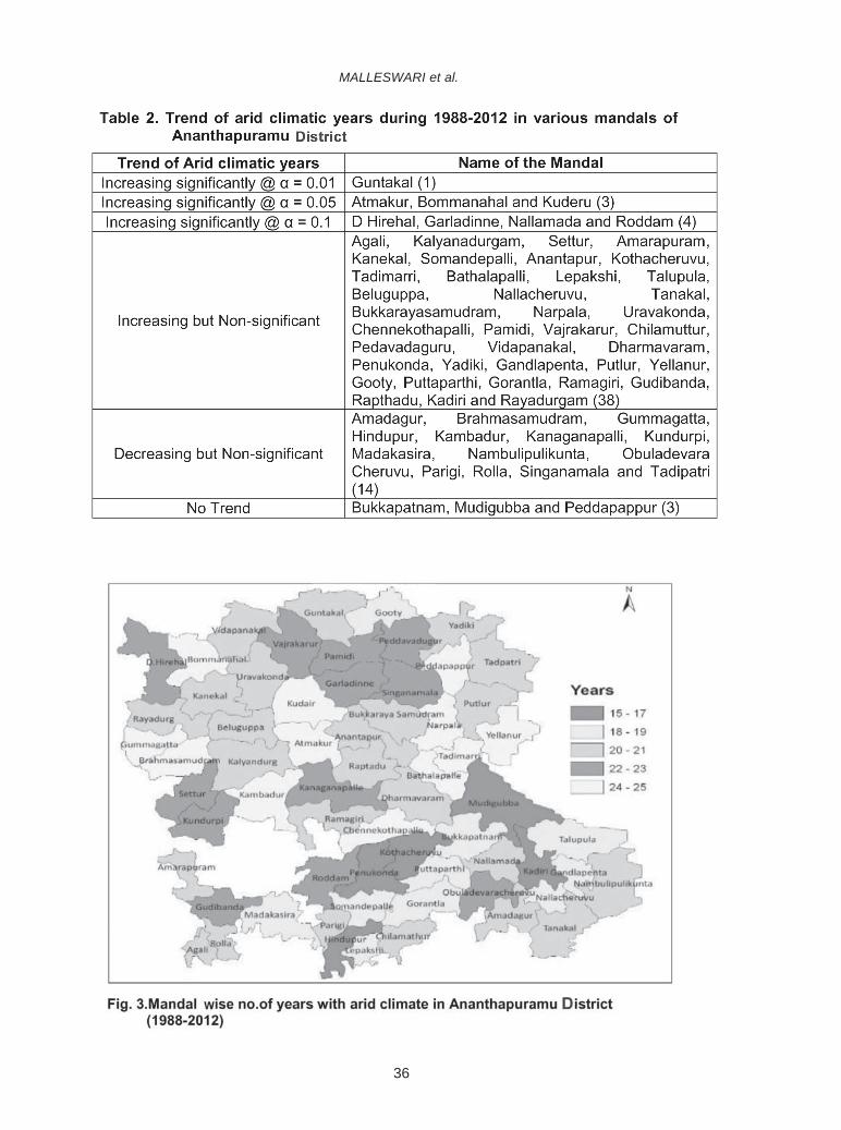
36
MALLESWARI et al.

37
MICRO LEVEL CLIMATIC CLASSIFICATION FOR ANANTHAPURAMU DISTRICT
They opined that there is a need to revise climaticclassification at least once in 30 years; may be morefrequently in future since more warming trends havebeen projected for future. Such an exercise may helpin knowing the spatial shifts of climatic zones, whichhas bigger implications for crop planning, waterresources assessment and launching of specialschemes on drought including disaster management.
CONCLUSION
Based on the investigation it could be statedthat there is an immediate need to concentrate oncontingency crop planning and drought preparednessin Guntakal, Atmakur, Bommanahal, Kuderu, DHirehal, Garladinne, Nallamada, Roddam,Pedavadagur, Peddapappur, CK Palli, Yellanurmandalsof Ananthapuramu district. Also, “weatherindices” shall be developed for crops rather than“climate indices” for successful growth of crops asclimate indices are ‘annual’ indices and do not fit forcrop health management thereby yields.
REFERENCES
Bhattacharjee, J, C., Roy Chaudhury, C., Landey,R, J and Pandey, S. 1982.BioclimaticAnalysis of India. NBSSLUP Bulletin. 7.Nagpur, India. pp.21.
Krishna Kumar, K., Patwardhan, S, K., Kulkarni, A.,Kamala, K., Koteswara Rao, K and Jones,R.2011. Simulated projections for summermonsoon climate over India high by aresolution regional climate model(PRECIS). Current Science.101:312–326.
Krishnan, A. 1988. Delineation of soil climatic zonesof India and its application in agriculture.Fertilizer News.33:11–19.
Raju, B.M. K., Rao, K, V., Venkateswarlu, B., Rao,A. V. M .S., Rama Rao, C. A., Rao, V. U.M., Bapuji Rao, B., Ravi Kumar, N., Dhakar,R., Swapna, N and Latha, P. 2013.Revisiting climatic classification in India :A district level analysis. CurrentScience.105 (4): 492-495.
Rao, K. N., George, C. J and Ramasastri, K. S.1972.Agroclimatic Classification of India.Agricultural Meteorology Division, IndiaMeteorological Department, Pune, India.
Salmi, T., Maatta, A., Anttila, P., Ruoho-Airola, T andAmnell, T. 2002. Detecting trends of annualvalues of atmospheric pollutants by theMann-Kendall test and Sen’s SlopeEstimates – the Excel Template ApplicationMAKESENS. Publications on Air QualityNo. 31. Finnish Meteorological Institute,Helsinki, Finland.pp.12-15.
Thornthwaite, C. W and Mather, J. R .1955.The waterbalance. Publications in Climatology.Drexel Institute of Technology, Laboratoryof Climatology, Centerton, New Jersey. 8(1):82-86.
Venkataraman, S and Krishnan, A. 1992. Crops andWeather. Publications and InformationDivision, Indian Council of AgriculturalResearch, New Delhi. pp.586.

38
INTRODUCTION
Potassium is one of major and essentialplant nutrients has instrumental role in plant nutritionand physiology. Many chemical methods such as1N NH4OAc, Mehlich-3, salts and dilute acids werestudied by researchers for evaluation of availablepotassium (K) in soils (Srinivasa Rao and Takkar,1997 and Mehta et al., 2001). Though, N N NH4OAcis a better extractant for assessing available K statusof soils has been reported by number of workers,the results obtained under AICRP on croppingsystems indicated that the response to applied Khave been observed in soils analyzing high inavailable K. Potassic fertilizer scheduling is done onthe basis of available K in soil measured by N NNH4OAc. A pot culture study was conducted toquantify the role of potassium required for plantgrowth using maize as test crop. To evaluate therelative efficiency of extractants with reference to dry
COMPARISION OF EXTRACTANTS TO ASSESS POTASSIUM AVAILABILITY INSOILS OF MAJOR CROPPING SYSTEMS IN KURNOOL DISTRICT
I.RAJEEVANA, P.KAVITHA, M.SREENIVASA CHARI AND M.SRINIVASA REDDYDepartment of Soil Science and Agricultural Chemistry,
Agricultural College, Acharya N.G. Ranga Agricultural University, Mahanandi- 518 501
Date of Receipt: 21.2.2017 Date of Acceptance:04.4.2017
ABSTRACT Sixty representative surface soil samples (0-15 cm) were collected during 2015-16 from five major cropping systems
(viz., rice-rice, fallow-bengalgram, groundnut-groundnut maize-maize, rice-maize/mustard) covering 13 mandals in Kurnool districtto compare the extractants to assess potassium availability in relation with K uptake studies in soils of major cropping systems.Thesoils under study were moderately coarse to fine in texture neutral to slightly alkaline, non saline and non-calcareous. Among theextractants tried, the relative efficiency of K releasing extractants were in the order: 1 N HNO3 > Mehilich-3 > N .N NH4OAc >0.01M CaCl2 > distilled water. Highest amount of potassium was extracted in maize-maize cropping system and lowest ingroundnut-groundnut cropping system with all the extractants. Relative efficiency of extractants also evaluated with referenceto dry matter yield, content and uptake of K by maize crop. All these K extractants were positively correlated with each other,though these extractants removed different quantities of K. The plant parameters i.e. dry matter; K content and K uptake of maizecrop were highest in maize-maize cropping system and lowest in groundnut –groundnut cropping system with the all extractants.Among the 5 extractants tried, 1N HNO3 showed the highest significant and positive correlation with yield (0.897**), content(0.890**) and uptake (0.933**) of potassium of maize crop followed by N NH4OAc and Mehilich-3. The highest positive andsignificant correlation of plant parameters was found with N N NH4OAc followed by 1 N HNO3 in maize-maize cropping system,fallow-bengal gram cropping system and groundnut-groundnut cropping system, whereas, incase of rice-maize/mustard croppingsystem and rice-rice cropping system 1 N HNO3 showed the highest correlation with plant parameters followed by N N NH4OAc.A close observation of the data indicated that 1 N HNO3 can be used along with N N NH4OAc for assessing available potassium insoils of major cropping systems in Kurnool district.
E-mail: [email protected]
J.Res. ANGRAU 45(2) 38-49, 2017
matter yield, K content and uptake of K. The role ofpotassium may vary from crop to crop and soil tosoil, mainly due to existence of variation in agroclimatic zones and nature of soil minerals supplyingthe nutrient. The information exclusively on soilsunder different cropping systems is in adequate. Thepresent investigation was conducted on majorcropping systems in Kurnool district to study the Kstatus and to evaluate the relative efficiency of anextractant for available potassium in the soil forsupplementing the crop with proper amounts offertilizer K.
MATERIAL AND METHODS
The study was undertaken in the Departmentof Soil Science and Agricultural Chemistry,Agricultural College, Mahanandi during the year2015-16. Sixty representative surface soil samples(0-15 cm) in bulk were collected from five cropping
39
systems (black and red soils viz. rice-rice, rice-maize/mustard, maize-maize, fallow-bengalgram,groundnut-groundnut in Kurnool district. Soil sampleswere extracted with neutral normal ammoniumacetate for K status. Based on K content 30 soilsamples are selected for K studies. The soil samplescollected were air dried and passed through 2 mmsieve. Each sample was then sub-sampled, byquartering and finally a representative soil samplewas preserved in a polythene bag for laboratoryanalysis. The selected soils were analyzed for theirintial soil properties and potassium releasecharacteristics. The particle size analysis wascarried out by Bouyoucous hydrometer method. ThepH and EC were determined in 1:2 soils, watersuspension using pH meter and EC meter. The freeCaCO3 content was determined as per proceduregiven by Piper. The texture of the soils has rangedfrom sandy loam to clay and moderately coarse tofine texture. Water soluble potassium wasdetermined in 1:5 soil: water extract, after 5 minutesequilibration and potassium in the aliquot wasdetermined by flame photometer. Potassium wasextracted in the N N NH4OAc (soil: extractant ratioof 1:5 equilibrating for 5 min) and the potassium inthe aliquot was determined by flame photometer. Thepotassium was estimated by boiling the soil with 1NHNO3 (soil: acid ratio 1:10) for 10 minutes and the Kcontent in the aliquot was determined by flamephotometer. Potassium was extracted with 0.01 M(calcium chloride (soil: extractant ratio of 1:10,equilibrating for 30 min) and the potassium in thealiquot was determined by flame photometer(Srinivasa Rao and Takkar, 1997). Potassium wasextracted with 0.02 M CH3COOH, 0.25 M NH4NO3,and 0.015 M NH4F, 0.013 M HNO3 and 0.001M EDTA(Mehilich-3) maintaining 1:10 soil: extractant ratioequilibrating for 5 minutes. The potassium in theextract was determined by flame photometer. A pot
culture experiment was conducted (by using 5 Kgeach of 2.0 mm sieved soil of different croppingsystem were taken in earthen pots) and P-3396maize hybrid was used as test crop. A commonrecommended dose of nitrogen and phosphorousapplied to all the treatments as per recommendeddose 250 N and 60 Kg ha-1 P2O5, respectively.Potassium was not applied to crop. The maizeseedlings @ three per pot were sown in each pot.Two plants were removed at 10 DAS and incorporatedin same pot so that only one plant was maintainedin each pot and the crop is harvested at 60 DAS.Plant samples collected at 60 DAS were processedand subjected to the tri acid digestion mixture ofHNO3: HClO4: H2SO4 (9:4:1) and the K content wasdetermined by using flame photometer. The drymatter and K content were determined. Thepotassium uptake was calculated using the followingformula and expressed in g pot-1.
Nutrient content (%) × Dry matter production (g pot -1)
Nutrient uptake (g pot -1) = —————————
100
RESULTS AND DISCUSSION
The pH of soils used in the study varied from6.9 in red soils of Yembavi in groundnut-groundnutcropping system to 8.4 in black soils ofBheemunipadu of rice-mustard cropping system(Table1 ), indicating that soils under investigationwere neutral to slightly alkaline. The electricalconductivity of soils ranged from 0.10 dSm-1 in redsoils of Yembavi of groundnut-groundnut croppingsystem to 0.69 dSm-1 in black soils ofVenkateswarapuram in fallow bengalgram croppingsystem with a mean value of 0.31 dSm-1, soils werenon-saline and non-calcareous. The texture of thesoils varied from moderately coarse to fine in texturei.e. sandy loam to clay (Table 1).
RAJEEVANA et al.

40
Distilled water extractable K
The highest mean distilled water extractablepotassium was observed in rice-mustard/maizecropping system (17 mg kg-1) followed by maize-maize cropping system (16 mg kg-1), rice-ricecropping system (13 mg kg-1), fallow bengalgramcropping system (9 mg kg-1) and lowest in groundnut-groundnut cropping system (7 mg kg-1) (Table 2).The distilled water extracted lower amounts of K thanthat of the other extractants because distilled wateris the softest extractant possible (Rathore et al.,2000). This was in conformity with the results of SivaPrasad (2014).
0.01 M CaCl2 extractable K
The mean value of 0.01 M CaCl2 extractablepotassium was higher in rice-rice cropping system(50 mg kg-1) followed by maize-maize croppingsystem (39 mg kg-1) , rice-mustard/maize croppingsystem (38 mg kg-1), fallow bengal gram croppingsystem (33 mg kg-1) and the lower values werenoticed in groundnut-groundnut cropping system (20mg kg-1) (Table 2).
The potassium extracted with 0.01 M CaCl2is lower than N.N.NH4OAc and high compared todistilled water. Generally soils with high clay contentshow high K release with dilute salt solution. Similarfindings were reported by Srinivasa Rao and Takkar(1997). Lakshminarayana et al. (2011) also foundlowest amount of available K with 0.01 M CaCl2 thanthat of 1N HNO3 and N.N NH4OAc, which might bedue to its low solubilization effect on nonexchangeable and lattice K forms. Similar reportswere also made by Bedi et al. (2002).
N.N. NH4OAc extractable K
Ammonium acetate was the most commonlyused extractant, which extracts, both exchangeableand water soluble K. The highest mean available form
of potassium was higher in maize-maize croppingsystem (357mg kg-1) followed by fallow bengal gramcropping system (292 mg kg-1), rice-mustard/maizecropping system (269 mg kg-1), rice-rice croppingsystem (182 mg kg-1) while the lower value werefound in groundnut-groundnut cropping system (153mg kg-1) (Table 2).
Mehilich-3 extractable-K
The mean value of Mehilich-3 extractablepotassium was higher in maize-maize croppingsystem (403 mg kg-1) followed by fallow bengal gramsystem (337 mg kg-1), rice-mustard/maize croppingsystem (300 mg kg-1) and rice-rice cropping system(238 mg kg-1) and the lower value were recorded ingroundnut-groundnut cropping system (201 mgkg-1) (Table 2).
1 N Boiling HNO3 extractable K
The mean value of 1 N Boiling HNO3
extractable potassium was found to be higher inmaize-maize cropping system (770 mg kg-1) followedby fallow bengal gram system (639 mg kg-1), rice-mustard/maize cropping system (534 mg kg-1) , rice-rice cropping system (417 mg kg-1) and lower valueswere noticed in groundnut-groundnut croppingsystem (358 mg kg-1) (Table 2). Among all theextractants, significantly higher amounts of K wereextracted by 1 N HNO3 because in addition toexchangeable K, some of the non-exchangeable Kis brought into solution by the breakdown of primaryand secondary clay minerals (Pati Ram and Prasad,1983). The mineral acids release more K than organicacids since mineral acids add higher H+ activity forthe same concentration and were obviously moreeffective in solubilising potassium from minerals(Ghosh, 1985). Similar findings were also reportedby Singh et al. (1992); Kalyani (2012). On the basisof extractability of potassium the extractants werein the order of r; 1 N HNO3 > Mehilich-3 > N.N
COMPARISION OF SOIL EXTRACTANTS TO ASSESS POTASSIUM AVAILABILITY

41
NH4OAc > 0.01M CaCl2 > distilled water. Higheramounts of potassium were extracted in maize-maizecropping system while the lower amounts wererecorded in lowest in groundnut-groundnut croppingsystem with all the extractants.
Potassium study by pot culture studies
The plant parameters i.e. dry matter, Kcontent and K uptake of maize crop were highest inSrinagaram village of maize-maize cropping systemand lowest in Balapala palli village of groundnut –groundnut cropping system. A wide variation in plantparameters in different soils was observed due tothe variation in potassium supplying power of soils(Nath and Dey , 1982) and also observed the variationin dry matter yields in the alluvial soils of Assamand in Aridisols of Rajasthan (Sharma and Swami,2000). The value of dry mater varied from 9.63(Balapalapalli) to 44.26 g pot-1 (Srinagaram) with amean value of 26.35 g pot- 1 (Table 3). The percent Kcontent ranged from 1.35 per cent in Balapalapalli to3.50 per cent in Srinagaram with a average value of2.30 percent. Similarly the K uptake was ranged from0.13 g pot-1 in Balapalapalli to 1.55 g pot-1 inSrinagaram with a mean of 0.65 g pot-1 .
Correlation coefficients (r) among the extractantsof potassium
The data presented in the Table 4 showsthat the variability in the amount of potassiumextracted between these methods is attributed tothe concentration of extractant. These extractantsdesorbed solution, exchangeable, non-exchangeableand some of the lattice K. The correlation coefficientsbetween K extracted by these chemical methodsare shown in the Table 4. All these K extractantswere positively correlated with each other, thoughthese extractants removed different quantities of Kwhich indicated that these methods can be used for
assessment of availability of K in present investigatedsoils and also amount of potassium extracted werecomparable. Similar reports were made by Bedi etal. (2002).
Correlation co-efficient (r) between extractingagents and plant parameters
Among the 5 extractants tried, 1N HNO3
showed maximum positive and significant correlationwith yield, content and uptake of potassium of maizecrop followed by N NH4OAc and Mehilich-3 (Table5). The relative efficiency of the extractants amongthe different cropping systems was studied byworking out correlation co-efficient betweenextractants and plant parameters and data waspresented in the Tables 6 to 10. The data revealedthat the higher significant and positive correlation ofplant parameters was found with N N NH4OAcfollowed by 1 N HNO3 in maize-maize croppingsystem, fallow-Bengal gram cropping system andgroundnut-groundnut cropping system. In case ofrice-maize/mustard cropping system and rice-ricecropping system, 1 N HNO3 showed the higherpositive and significant correlation with plantparameters followed by N N NH4OAc. These resultsare in conformity with the findings of Liangxue andBates (1990). Siva Prasad (2014) also reported thatamong the eight extractants tried, 1N HNO3 showedhigh positive correlation with dry matter yields anduptake of shoot and whole plant and also showedpositively significant correlation with the shoot Kcontent of bajra crop in Neubauer’s rapid seedlingtechnique followed by Mehilich-3 and N NH4OAc.Similar reports were given by Swamanna (2015). Aclose observation of the data indicated that 1 N HNO3
can be used along with N N NH4OAc for assessingavailable potassium in soils of major croppingsystems in Kurnool district.
RAJEEVANA et al.

42
S.
ECC
aNo
Villa
ge N
ame
Cro
ppin
g sy
stem
GPS
coo
rdin
ates
pH(d
SCO
3O
.CTe
xtur
em
-1)
(%)
(mg)
1R
ARS,
Nan
dyal
Ric
e-ric
eN
:150 2
8.50
0
E:0
780 3
0.15
98.
20.
220.
680.
47C
lay
2Ba
ttalu
ruR
ice-
rice
N:1
50 14.
102
E
:078
0 28.
127
8.1
0.46
0.49
0.43
Silt
y lo
am
3N
alla
gatla
Ric
e-ric
eN
:150 1
3.21
9
E:0
780 3
0.15
77.
90.
202.
270.
44S
ilty
clay
loam
4Ka
min
enip
alli
Ric
e-ric
eN
:150 2
3.47
9
E:0
780 3
3.19
77.
50.
180.
220.
27Lo
am
5Ye
rragu
didi
nna
Ric
e-ric
eN
:150 1
1.18
6
E:0
780 3
1.91
27.
40.
212.
720.
36S
ilty
clay
loam
6M
.C. f
arm
Ric
e-ric
eN
:150 2
5.57
7
E:0
780 2
2.56
37.
30.
321.
580.
46S
andy
loa
m
7Sr
inag
aram
Mai
ze-m
aize
N:1
50 27.
141
E
:078
0 33.
734
8.3
0.68
0.22
0.44
San
dy c
lay
loam
8Ta
mad
apal
liM
aize
-mai
zeN
:150 2
8.52
4
E:0
780 3
2.90
08.
10.
270.
220.
55S
ilty
clay
loam
9Ve
lpan
uru
Mai
ze-m
aize
N:1
50 42.
042
E
:078
0 31.
273
8.2
0.20
1.36
0.46
San
dy c
lay
10M
ahan
andi
Mai
ze-m
aize
N:1
50 26.
212
E
:078
0 37.
344
7.9
0.20
1.59
0.45
Silt
y cl
ay lo
am
11N
alla
kalv
aM
aize
-mai
zeN
:150 5
2.56
8
E:0
780 4
1.42
57.
20.
172.
040.
34Lo
am
12M
.C.fa
rmM
aize
-mai
zeN
:150 2
8.41
6
E:0
780 2
3.49
27.
40.
181.
450.
48S
andy
loam
13Ka
nala
Ric
e-m
usta
rdN
:150 2
5.81
4
E:0
780 2
7.58
18.
20.
190.
900.
39S
ilty
clay
loam
14Bh
emun
ipad
uR
ice-
mus
tard
N:1
50 23.
.332
E
:078
0 31.
676
8.4
0.55
2.07
0.33
San
dy c
lay
loam
15Bo
llava
ram
Ric
e-m
aize
N:1
50 27.
512
E
:078
0 24.
421
7.9
0.30
2.32
0.41
San
dy c
lay
loam
16R
ythu
naga
ram
Ric
e-m
usta
rdN
:150 2
8.40
6
E:0
780 3
2.47
57.
30.
570.
450.
43Lo
am
17Ay
yava
rikod
uru
Ric
e-m
aize
N:1
50 31.
234
E
:078
0 31.
687.
20.
221.
810.
44S
andy
cla
y lo
am
18G
ajul
apal
liR
ice-
mai
zeN
:150 2
4.26
3
E:0
780 3
8.04
67.
50.
102.
120.
41S
andy
cla
y lo
am
19R
ARS,
Nan
dyal
Fallo
w b
enga
lgra
mN
:150 2
8.15
0
E:0
780 3
0.22
98.
10.
682.
040.
50S
ilty
clay
loam
20Ve
nkat
eswa
rwpu
ram
Fallo
w b
enga
lgra
mN
:150 3
2.34
0
E:0
780 2
2.56
38.
30.
691.
680.
51S
ilty
clay
loam
Tabl
e 1.
Phy
sico
-che
mic
al p
rope
rtie
s of
exp
erim
enta
l soi
ls
Con
td...
COMPARISION OF SOIL EXTRACTANTS TO ASSESS POTASSIUM AVAILABILITY

43
S.
ECC
aNo
Villa
ge N
ame
Cro
ppin
g sy
stem
GPS
coo
rdin
ates
pH(d
SCO
3O
.CTe
xtur
em
-1)
(%)
(mg)
21N
erav
ada
Fallo
w b
enga
lgra
mN
:150 3
3.75
2
E:0
780 2
4.79
38.
00.
171.
130.
48S
ilty
loam
22Ba
lapa
nuru
Fallo
w b
enga
lgra
mN
:150 2
9.91
8
E:0
780 2
0.19
78.
20.
261.
810.
47S
ilty
clay
loam
23Ko
ulur
uFa
llow
ben
galg
ram
N:1
50 33.
334
E
:078
0 25.
194
8.0
0.21
0.90
0.53
Silt
y cl
ay lo
am
24Bo
yire
vula
Fallo
w b
enga
lgra
mN
:150 4
1.09
7
E:0
780 3
3.61
67.
80.
310.
180.
34S
andy
cla
y lo
am
25M
.C.fa
rmG
roun
dnut
-gro
undn
utN
:150 5
3.12
1
E:0
780 3
3.37
47.
40.
11.
0.45
0.27
San
dy lo
am
26Sh
anka
rapa
lliG
roun
dnut
-gro
undn
utN
:150 5
2.67
2
E:0
770 6
2.47
27.
10.
190.
900.
27S
andy
loam
27M
udda
ram
Gro
undn
ut-g
roun
dnut
N:1
50 53.
451
E
:077
0 66.
537
7.2
0.14
0.22
0.21
San
dy lo
am
28Ba
lapu
ram
Gro
undn
ut-g
roun
dnut
N:1
50 54.
326
E
:077
0 63.
612
7.1
0.26
5.21
0.42
Loam
29Ba
lapa
lapa
lliG
roun
dnut
-gro
undn
utN
:150 5
5.25
1
E:0
770 7
1.69
17.
20.
660.
220.
34S
andy
loam
30Ye
mba
viG
roun
dnut
-gro
undn
utN
:150 4
8.78
0
E:0
780 2
1.42
06.
90.
102.
720.
24S
andy
loam
M
ean
0.31
2.13
0.40
RAJEEVANA et al.C
ontd
...

44
1 RARS, Nandyal R-R 12 51 225 353 5702 Battaluru R-R 12 31 190 210 3873 Nallagatla R-R 16 65 183 256 4284 Kaminenipalli R-R 11 34 82 106 2105 Yerragudidinna R-R 10 46 130 184 2706 M.C. farm R-R 17 70 279 320 635
Mean 13 50 182 238 4177 Srinagaram M-M 22 40 779 820 15868 Tamadapalli M-M 15 45 338 394 7309 Velpanuru M-M 14 38 355 376 852
10 Mahanandi M-M 13 36 215 265 41611 Nallakalva M-M 9 25 131 172 33112 M.C.farm M-M 20 48 326 392 703
Mean 16 39 357 403 77013 Kanala R-MU 9 18 246 268 36414 Bhemunipadu R-MU 13 37‘ 131 124 26815 Rythunagaram R-MU 21 48 357 404 75816 Bollavaram R-MA 11 26 371 415 82017 Ayyavarikoduru R-MA 18 40 206 221 32818 Gajulapalli R-MA 28 57 305 365 668
Mean 17 38 269 300 53419 RARS, Nandyal FB 8 36 261 303 62320 Venkateswarwpuram FB 11 45 362 402 85321 Neravada FB 6 31 210 278 45322 Balapanuru FB 10 26 326 390 68023 Kouluru FB 13 38 475 515 96024 Boyirevula FB 5 23 117 136 267
Mean 9 33 292 337 63925 M.C.farm GN-GN 8 18 201 264 42126 Shankarapalli GN-GN 10 23 203 243 43627 Muddaram GN-GN 6 15 71.5 101 18928 Balapuram GN-GN 7 24 301 375 74129 Balapalapalli GN-GN 8 17 57.5 102 16630 Yembavi GN-GN 5 25 81 119 193
Mean 7 20 153 201 358
Table 2. Efficiency of different extracting agents of potassium in soils of major cropping systems in Kurnool district (mg kg-1 soil)
R- R: rice-rice, M-M: maize-maize, R-MA: rice-maize, R-MU: rice-mustard, FB: fallowbengalgram,GN-GN:groundnut-groundnut
S.No
Village name Croppingsystem
Distilledwater
extractableK
0.01MCaCl2
extractableK
N NNH4OAC
extractableK
Mehilich 3extra
ctable K
1N boilingHNO3
extractableK
COMPARISION OF SOIL EXTRACTANTS TO ASSESS POTASSIUM AVAILABILITY

45
Table 3. Dry matter, K content and K uptake of maize crop in studied soils
S.No Village Name Drymatter K content K uptake(g pot-1) (%) (g pot -1)
1 RARS, Nandyal rice 28.91 2.20 0.64
2 Battaluru 27.86 2.03 0.57
3 Nallagatla 25.98 2.08 0.54
4 Kaminenipalli 11.74 1.45 0.17
5 Yerragudidinna 23.99 1.95 0.47
6 M.C. farm, rice 32.07 2.59 0.83
7 Srinagaram 44.26 3.50 1.55
8 Tamadapalli 34.89 2.70 0.94
9 Velpanuru 35.98 3.25 1.17
10 Mahanandi 25.05 2.35 0.59
11 Nallakalva 21.76 1.91 0.42
12 M.C. farm, maize 33.35 2.70 0.90
13 Kanala 26.77 2.46 0.66
14 Bhemunipadu 18.37 1.73 0.32
15 Rythunagaram 33.36 3.21 1.07
16 Bollavaram 36.06 3.20 1.15
17 Ayyavarikoduru 23.19 2.03 0.47
18 Gajulapalli 29.47 2.33 0.69
19 RARS,Nandyal Bengalgram 28.42 2.35 0.67
20 Venkateswarwpuram 32.37 2.95 0.95
21 Neravada 24.99 2.26 0.56
22 Balapanuru 31.36 2.45 0.77
23 Kouluru 38.16 2.75 1.05
24 Boyirevula 14.37 1.71 0.02
25 M.C.farm, groundnut 22.84 2.15 0.49
26 Shankarapalli 24.80 2.24 0.56
27 Muddaram 10.52 1.41 0.15
28 Balapuram 28.93 2.40 0.69
29 Balapalapalli 9.63 1.35 0.13
30 Yembavi 11.17 1.40 0.16
Mean 26.35 2.30 0.65
RAJEEVANA et al.

46
Table 4. Inter correlations between different extractants
Distilled 0.01M 1N NH4OAc Mehilich- 3 1 N HNO3
water K CaCl2 K K K K
Distilled water K 1.000
0.01M CaCl2 K 0.708** 1.000
1N NH4OAc K 0.480** 0.292 1.000
Mehilich- 3 K 0.534** 0.329*** 0.986** 1.000
1 N HNO3 K 0.400* 0.331*** 0.950** 0.987** 1.000
* Significant at 0.05 per cent level; **Significant at 0.01 per cent level ***Significant at 0.1 per cent level
Table 5. Correlation co-efficient (r) between different extractants and plant parameters
Dry matter K content K uptake
Distilled water 0.556** 0.507** 0.556**
0.01M CaCl2 0.466** 0.358* 0.391*
1N NH4OAc 0.896** 0.887** 0.931**
Mehilich- 3 0.889** 0.885** 0.927**
1 N HNO3 0.897** 0.890** 0.933**
*Significant at 0.05 per cent level; **Significant at 0.01 per cent level
Table 6. Correlation co-efficient (r) between different extractants of K and plant parameters in rice-rice cropping system
Dry matter K content K uptake
Distilled water 0.841** 0.751** 0.798**
0.01M CaCl2 0.623** 0.533** 0.511**
1N NH4OAc 0.923** 0.869** 0.939**
Mehilich- 3 0.920** 0.852** 0.926**
1 N HNO3 0.945** 0.902** 0.964**
**Significant at 0.01 per cent level
COMPARISION OF SOIL EXTRACTANTS TO ASSESS POTASSIUM AVAILABILITY
Extractants
ExtractantsPlant parameters
ExtractantsPlant parameters

47
Table 7. Correlation co-efficient (r) between different extractants of K and plant parameters of maize-maize cropping system
Dry matter K content K uptake
Distilled water 0.541** 0.693** 0.642**
0.01M CaCl2 0.572** 0.74** 0.66**
1N NH4OAc 0.912** 0.961** 0.971**
Mehilich- 3 0.854** 0.872** 0.879**
1 N HNO3 0.846** 0.917** 0.912**
**Significant at 0.01 per cent level
Table 8. Correlation co-efficient (r) between different extractants of K and plant parameters of rice-maize/rice mustard cropping system
Dry matter K content K uptake
Distilled water 0.936** 0.880** 0.914**
0.01M CaCl2 0.676** 0.858** 0.759**
1N NH4OAc 0.969** 0.887** 0.944**
Mehilich- 3 0.986** 0.895** 0.965**
1 N HNO3 0.966** 0.942** 0.964**
**Significant at 0.01 per cent level
Table 9. Correlation co-efficient (r) between different extractants of K and plant parameters of fallow-bengal gram cropping system
Dry matter K content K uptake
Distilled water 0.140NS -0.01 NS 0.02NS
0.01M CaCl2 0.04NS -0.13 NS -0.07 NS
1N NH4OAc 0.991** 0.941** 0.962**
Mehilich- 3 0.981** 0.907** 0.933**
1 N HNO3 0.946** 0.880** 0.925**
**Significant at 0.01 per cent level ; NS- Non- significant
RAJEEVANA et al.
ExtractantsPlant parameters
ExtractantsPlant parameters
ExtractantsPlant parameters
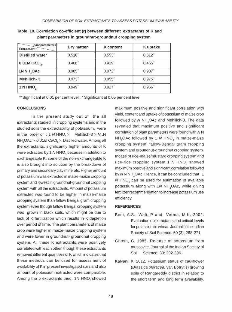
48
CONCLUSIONS
In the present study out of the allextractants studied in cropping systems and in thestudied soils the extractability of potassium, werein the order of : 1 N HNO3 > Mehilich-3 > N .NNH4OAc > 0.01M CaCl2 > Distilled water. Among allthe extractants, significantly higher amounts of Kwere extracted by 1 N HNO3 because in addition toexchangeable K, some of the non-exchangeable Kis also brought into solution by the breakdown ofprimary and secondary clay minerals. Higher amountof potassium was extracted in maize-maize croppingsystem and lowest in groundnut-groundnut croppingsystem with all the extractants. Amount of potassiumextracted was found to be higher in maize-maizecropping system than fallow Bengal gram croppingsystem even though fallow Bengal cropping systemwas grown in black soils, which might be due tolack of K fertilization which results in K depletionover period of time. The plant parameters of maizecrop were higher in maize-maize cropping systemand were lower in groundnut- groundnut croppingsystem. All these K extractants were positivelycorrelated with each other, though these extractantsremoved different quantities of K which indicates thatthese methods can be used for assessment ofavailability of K in present investigated soils and alsoamount of potassium extracted were comparable.Among the 5 extractants tried, 1N HNO3 showed
maximum positive and significant correlation withyield, content and uptake of potassium of maize cropfollowed by N NH4OAc and Mehilich-3. The datarevealed that maximum positive and significantcorrelation of plant parameters were found with N NNH4OAc followed by 1 N HNO3 in maize-maizecropping system, fallow-Bengal gram croppingsystem and groundnut-groundnut cropping system.Incase of rice-maize/mustard cropping system andrice-rice cropping system 1 N HNO3 showedmaximum positive and significant correlation followedby N N NH4OAc. Hence, it can be concluded that 1N HNO3 can be used for estimation of availablepotassium along with 1N NH4OAc, while givingfertilizer recommendation to increase potassium useefficiency.
REFERENCES
Bedi, A.S., Wali, P and Verma, M.K. 2002.Evaluation of extractants and critical levelsfor potassium in wheat. Journal of the IndianSociety of Soil Science. 50 (3): 268-271.
Ghosh, G. 1985. Release of potassium frommuscovite. Journal of the Indian Society ofSoil Science. 33: 392-396.
Kalyani, K. 2012. Potassium status of cauliflower(Brassica oleracea. var. Botrytis) growingsoils of Rangareddy district in relation tothe short term and long term availability.
Table 10. Correlation co-efficient (r) between different extractants of K and plant parameters in groundnut-groundnut cropping system
Dry matter K content K uptake
Distilled water 0.510** 0.553** 0.512**
0.01M CaCl2 0.466** 0.419* 0.465**
1N NH4OAc 0.985** 0.972** 0.987**
Mehilich- 3 0.973** 0.955** 0.975**
1 N HNO3 0.949** 0.927** 0.956**
**Significant at 0.01 per cent level ; * Significant at 0.05 per cent level
COMPARISION OF SOIL EXTRACTANTS TO ASSESS POTASSIUM AVAILABILITY
ExtractantsPlant parameters
49
M.Sc. Thesis submitted to Acharya N.G.Ranga Agricultural University, Hyderabad,India.
Laxminarayana, K., Sanjeebbharali and Patiram.2011. Evaluation of chemical extractionmethods for available potassium in ricesoils of Meghalaya. Journal of the IndianSociety of Soil Science. 59 (3): 295-299.
Liangxue, L and Bates, E.T. 1990. Evaluation of soilextractants for the prediction of plantavailable potassium in Ontario soils.Canadian Journal of Soil Science. 70: 607-615.
Mehta, S.C., Shiel, R.S., Grewal, K.S and Mittal,S.B. 2001. Relative efficiency of differentextractants for non-exchangeable K releasein soils. Journal of Potassium Research.17:48-5l.
Nath, A. K and Dey, S.K. 1982.Studies on potassiumrelease pattern in various textural types ofalluvial soils of Assam by the methods ofexhaustive cropping. Journal of the IndianSociety of Soil Science.27:268-271.
Pati Ram and Prasad, R.N. 1983. Potassiumsupplying power of soils from the East Khasihills of Meghalaya. Journal of the IndianSociety of Soil Science.31: 506-510.
Rathore, H. S., Khatri, P. B and Swami, B. N. 2000.Comparision of methods of availablepotassium assessment for Ustochrepts inRajasthan. Journal of Indian Society of SoilScience. 48 (2): 621-623.
Sharma, R.K and Swami, B.N.2000. Studies on Kreleasing capacity of Aridisols of Rajasthan.Agropedology.10:67-74.
Siva Prasad, P.N. 2014. Studies on availablepotassium in rice (Oryza sativa L.) growingsoils of canal ayacut in kurnool district.M.Sc. Thesis submited to Acharya N.G.Ranga Agricultural University, Hyderabad.
Srinivasa Rao, Ch and Takkar, P.N. 1997. Evaluationof different extractants for measuring thesoil potassium determination of criticallevels for plant-available K in smectitic soilsfor Sorghum. Journal of the Indian Societyof Soil Science. 45(1): 113-119.
Swamanna, J. 2015. Potassium releasecharacteristics and response to potassiumapplication in rice (Oryza sativa L.) growingsoils of Kurnool district. M.Sc. Thesissubmitted to Professor JayashankarTelangana State Agricultural University.Hyderabad.
RAJEEVANA et al.

50
INTRODUCTION
The predominant cropping system in rainfedareas of Krishna agro-climatic zone of AndhraPradesh is with long duration crops such as cotton,chillies, etc under high input management. Withincreasing cost of cultivation and lower minimumsupport price, cotton and chilli farmers are under riskespecially in rainfed areas. The crops are also beingsubjected to abiotic and biotic stresses frequentlyresulting in farmers falling into debt trap andconsequent distress. The maize-chickpea sequenceis found to be profitable than sole crop and also helpsin soil fertility maintenance on long run in Krishnazone of Andhra Pradesh (Sharma and Behera, 2009).If this crop sequence is introduced to the Krishnaagro-climatic zone of Andhra Pradesh, it will bebeneficial in many ways. Both the crops togetherrequire comparatively shorter period to that of cottonand chilli and at the same time risk free with securedincome to the farmer and sustainable to the soilhealth. Maize and chickpea crops has good marketvalue and fetch higher prices than MSP announced
YIELD AND ECONOMICS OF MAIZE-CHICKPEA SEQUENCE AS INFLUENCED BYSOWING TIME AND NITROGEN LEVELS
M. RATNAM, B. VENKATESWARLU, E. NARAYANA, T.C.M NAIDU AND A. LALITHAKUMARI
Regional Agricultural Research Station,Acharya N.G. Ranga Agricultural University, Guntur-522 034
Date of Receipt: 28.2.2017 Date of Acceptance:19.4.2017
ABSTRACTA field experiment was conducted on clay soils of Regional Agricultural Research Station, Guntur during kharif and rabi
of 2013-14 and 2014-15 to find out the influence of sowing time and nitrogen levels on yield and economics of maize-chickpeasequence under rainfed agro-climatic condition of Krishna zone. Sowing time and nitrogen levels significantly influenced theeconomic yield of preceding maize and succeeding chickpea under of maize-chickpea sequence. From the sequence of precedingkharif maize followed by succeeding rabi chickpea, maximum net return of Rs.1,38,154 ha-1 and Rs.1,38,936 ha-1, respectivelyduring the first and the second year was obtained with 1st FN of July sowing with 200 % of Recommended Dose of Nitrogen (RDN)to preceding kharif maize and 100 % RDN to succeeding rabi chickpea followed by 2nd FN July sowing with 150 % RDN topreceding kharif maize and 75 % RDN to succeeding rabi chickpea. While ,the lower net return of Rs. 53,232 ha-1 and Rs. 50,919ha-1 were obtained with 2nd FN July sowing with 100% of RDN to preceding kharif maize and 0% RDN to succeeding rabi chickpea.The benefit-cost ratio of maize-chickpea sequence ranged from 1.1 to 3.6 in first year and 1.2 to 3.9 in the second year withdifferent treatments. The higher B:C ratio was obtained in 1st FN July sowing with 200 % RDN to preceding maize and 100% RDNto succeeding chickpea during both the years of experimentation.
E-mail: [email protected]
J.Res. ANGRAU 45(2) 50-58, 2017
by GoI (MSP-Maize: Rs. 1310 q-1 and Chickpea:Rs.3100 q-1, respectively) (CACP, 2013). Among themaize based cropping systems, maize-chickpea isone which is recently introduced due to the changingscenario of natural resource base. Therefore,introduction of maize-chickpea with appropriate inputmanagement under rainfed conditions of Krishna zonemay sustain the economy of the rainfed farmers.Hence, the present investigation was carried out tostudy the economic returns of the sequence.
MATERIAL AND METHODS
A field experiment was conducted atRegional Agricultural Research Station, Guntur(Latitude:160181, Longitude: 800291, Altitude:33 m).The climate is sub-tropical with mean annual rainfallof 950 mm. The soil of experimental field was clayloam in texture, neutral to slightly alkaline in reaction(pH 7.8 to 8.2) low in available N (204 kg ha-1), highin P2O5 (96.5 kg ha-1) and K2O (886.5 kg ha-1) andmedium in organic carbon (0.51%), respectively. Theexperiment was conducted for two successive kharifand rabi seasons of 2013-14 and 2014-15 in Krishnaagro-climatic zone of Andhra Pradesh. The
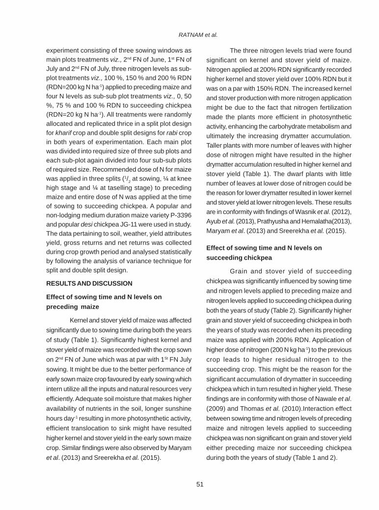
51
experiment consisting of three sowing windows asmain plots treatments viz., 2nd FN of June, 1st FN ofJuly and 2nd FN of July, three nitrogen levels as sub-plot treatments viz., 100 %, 150 % and 200 % RDN(RDN=200 kg N ha-1) applied to preceding maize andfour N levels as sub-sub plot treatments viz., 0, 50%, 75 % and 100 % RDN to succeeding chickpea(RDN=20 kg N ha-1). All treatments were randomlyallocated and replicated thrice in a split plot designfor kharif crop and double split designs for rabi cropin both years of experimentation. Each main plotwas divided into required size of three sub plots andeach sub-plot again divided into four sub-sub plotsof required size. Recommended dose of N for maizewas applied in three splits (1/2 at sowing, ¼ at kneehigh stage and ¼ at taselling stage) to precedingmaize and entire dose of N was applied at the timeof sowing to succeeding chickpea. A popular andnon-lodging medium duration maize variety P-3396and popular desi chickpea JG-11 were used in study.The data pertaining to soil, weather, yield attributesyield, gross returns and net returns was collectedduring crop growth period and analysed statisticallyby following the analysis of variance technique forsplit and double split design.
RESULTS AND DISCUSSION
Effect of sowing time and N levels onpreceding maize
Kernel and stover yield of maize was affectedsignificantly due to sowing time during both the yearsof study (Table 1). Significantly highest kernel andstover yield of maize was recorded with the crop sownon 2nd FN of June which was at par with 1St FN Julysowing. It might be due to the better performance ofearly sown maize crop favoured by early sowing whichintern utilize all the inputs and natural resources veryefficiently. Adequate soil moisture that makes higheravailability of nutrients in the soil, longer sunshinehours day-1 resulting in more photosynthetic activity,efficient translocation to sink might have resultedhigher kernel and stover yield in the early sown maizecrop. Similar findings were also observed by Maryamet al. (2013) and Sreerekha et al. (2015).
The three nitrogen levels triad were foundsignificant on kernel and stover yield of maize.Nitrogen applied at 200% RDN significantly recordedhigher kernel and stover yield over 100% RDN but itwas on a par with 150% RDN. The increased kerneland stover production with more nitrogen applicationmight be due to the fact that nitrogen fertilizationmade the plants more efficient in photosyntheticactivity, enhancing the carbohydrate metabolism andultimately the increasing drymatter accumulation.Taller plants with more number of leaves with higherdose of nitrogen might have resulted in the higherdrymatter accumulation resulted in higher kernel andstover yield (Table 1). The dwarf plants with littlenumber of leaves at lower dose of nitrogen could bethe reason for lower drymatter resulted in lower kerneland stover yield at lower nitrogen levels. These resultsare in conformity with findings of Wasnik et al. (2012),Ayub et al. (2013), Prathyusha and Hemalatha(2013),Maryam et al. (2013) and Sreerekha et al. (2015).
Effect of sowing time and N levels onsucceeding chickpea
Grain and stover yield of succeedingchickpea was significantly influenced by sowing timeand nitrogen levels applied to preceding maize andnitrogen levels applied to succeeding chickpea duringboth the years of study (Table 2). Significantly highergrain and stover yield of succeeding chickpea in boththe years of study was recorded when its precedingmaize was applied with 200% RDN. Application ofhigher dose of nitrogen (200 N kg ha-1) to the previouscrop leads to higher residual nitrogen to thesucceeding crop. This might be the reason for thesignificant accumulation of drymatter in succeedingchickpea which in turn resulted in higher yield. Thesefindings are in conformity with those of Nawale et al.(2009) and Thomas et al. (2010).Interaction effectbetween sowing time and nitrogen levels of precedingmaize and nitrogen levels applied to succeedingchickpea was non significant on grain and stover yieldeither preceding maize nor succeeding chickpeaduring both the years of study (Table 1 and 2).
RATNAM et al.

52
Economics of maize-chickpea sequence
Gross and net returns and benefit-cost ratiowere worked out for preceding maize, succeedingrabi chickpea separately and the system by takinginto consideration of all the inputs used in kharif andrabi seasons, and the economic yield for both theseasons during the two years of the study arepresented in (Table 3 and 4). From the sequence ofpreceding kharif maize followed by succeeding rabichickpea, maximum net return of Rs.1,38,154 ha-1
and Rs.1,38,936 ha-1, respectively during the firstand the second year was obtained with 1st FN ofJuly sowing with 200% of RDN to preceding kharifmaize and 100 % RDN to succeeding rabi chickpeafollowed by 2nd FN July sowing with 150% RDN topreceding kharif maize and 75% RDN to succeeding
Table 1. Kernel yield of maize as influenced by sowing time and nitrogen levels
Treatments drymatter accumulation Kernel yield Stover yield (g m-2) at harvest (q ha-1) (t ha-1)
2013 2014 2013 2014 2013 2014
Main Plots: Sowing time (A)
2nd FN of June 2094.11 1894.11 95.52 94.87 12.38 12.29
1st FN of July 1920.89 1720.89 93.48 92.83 11.14 10.99
2nd FN of July 1637.67 1437.67 77.71 77.06 10.55 10.40
SEm ± 52.78 74.71 3.19 3.18 0.40 0.45
CD @ 5% 207.24 207.42 12.52 12.50 1.58 1.77
C V % 8.40 9.41 10.76 10.84 10.65 12.03
Sub-plots: N Levels (B)
100 % RDN 1606.76 1406.78 81.40 80.75 9.48 9.38
150 % RDN 1936.11 1706.78 91.35 90.70 12.39 12.18
200 % RDN 2109.78 1909.78 93.96 93.31 12.20 12.11
SEm ± 68.06 96.23 2.61 2.61 0.37 0.39
CD @ 5 % 209.70 209.70 8.05 8.10 1.13 1.19
C V % 10.83 12.12 8.82 8.88 9.65 10.30
Interaction NS NS NS
NS - Non - Significant
rabi chickpea. While, the lower net return of Rs.53,232 ha-1 and Rs. 50, 919 ha-1 were obtained with2nd FN July sowing with 100% of RDN to precedingkharif maize and 0% RDN to succeeding rabichickpea. The benefit- cost ratio of maize chickpeasequence ranged from 1.1 to 3.6 in first year and 1.2to 3.9 in the second year with different treatments.The higher B:C ratio was obtained with 1st FN Julysowing with 200 % RDN to preceding maize and100% RDN to succeeding rabi chickpea. Higher yieldbenefiting higher return could be the reason for currentresults. These results are in accordance with thefindings of Saini and Vinod Kumar (2001), Moshaand Raghavaiah (2003), Nawale et al. (2009),Lingaraju et al. (2010), Jnanesha et al. (2012) andVidyavathi et al. (2011) and Mohankumar andHiremath (2015).
YIELD AND ECONOMICS OF MAIZE-CHICKPEA SEQUENCE

53
CONCLUSION
From the study it can be concluded thatsowing maize during 1st FN of July with 200 % RDNfollowed by 100 % RDN to succeeding chickpea wasfound to be the best in terms of yield of maize-chickpea sequence as well as economic returns fromthe system.
REFERENCESCACP. 2013. Minimum support prices recommended
by CACP and fixed by Government.Retrieved from website(www.cacp.dacnet.nic.in) on 10.2.2017.
Ayub, Muhammad, Tahir, Muhammad, Abrar,Muhammad and Khaliq, Abdul. 2013. Yieldand quality response of forage maize to
Table 2. Grain yield of succeeding chickpea as influenced by sowing time and nitrogen levels
Treatments drymatter accumulation Kernel yield Stover yield (g m-2) at harvest (q ha-1) (t ha-1)
2013-14 2014-15 2013-14 2014-15 2013-14 2014-15
Main plots: Maize sowing window (A)
2nd FN of June 193.59 183.84 13.39 13.25 1.34 1.92
1st FN of July 294.99 287.57 17.43 17.42 2.95 2.91
2nd FN of July 272.18 265.02 15.50 15.39 2.72 2.65
SEm ± 11.25 8.79 0.09 0.11 0.04 0.07
CD @ 5 % 38.26 34.43 0.28 0.34 0.12 0.22
CV (%) 5.30 20.44 2.72 3.34 7.12 13.47
Sub plots: N applied to maize
100% RDN 194.97 198.81 14.05 13.99 1.95 1.93
150% RDN 237.89 217.01 14.77 14.72 2.38 2.36
200% RDN 327.89 320.61 17.49 17.35 3.28 3.18
SEm ± 21.19 6.98 0.13 0.25 0.02 0.05
CD @ 5 % 64.28 21.49 0.38 0.76 0.07 0.15
CV (%) 3.73 17.00 4.80 9.70 4.89 12.04
sub-sub plots: N applied to chickpea
0 % RDN 224.88 215.60 1224 12.20 2.22 2.20
50 % RDN 249.49 240.95 1462 14.48 2.49 2.45
75 % RDN 265.82 257.87 1637 16.29 2.67 2.65
100 % RDN 274.16 267.47 1852 18.45 2.76 2.67
SEm ± 25.10 13.72 0.16 0.27 0.02 0.06
CD @ 5 % NS 45.04 0.49 0.82 0.07 0.19
CV (%) 9.49 6.95 5.90 9.81 4.18 19.98
Interaction NS NS NS
RATNAM et al.
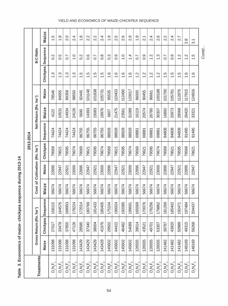
54
D1N
1F1
1310
9827
017
1581
1556
674
2289
579
569
7442
441
2278
546
1.3
0.2
1.5
D1N
1F2
1310
9833
478
1645
7656
674
2294
779
621
7442
410
531
8495
51.
30.
51.
8
D1N
1F3
1310
9837
855
1689
5356
674
2292
179
595
7442
414
934
8935
81.
30.
72.
0
D1N
1F4
1310
9847
126
1782
2456
674
2300
079
674
7442
424
126
9855
01.
31.
02.
4
D1N
2F1
1434
2928
585
1720
1456
674
2289
579
569
8675
556
9092
445
1.5
0.2
1.8
D1N
2F2
1434
2937
340
1807
6956
674
2294
779
621
8675
514
393
1011
481.
50.
62.
2
D1N
2F3
1434
2938
004
1814
3356
674
2292
179
595
8675
515
083
1018
381.
50.
72.
2
D1N
2F4
1434
2941
976
1854
0556
674
2300
079
674
8675
518
976
1057
311.
50.
82.
4
D1N
3F1
1456
0229
502
1751
0456
674
2289
579
569
8892
866
0795
535
1.6
0.3
1.9
D1N
3F2
1456
0244
422
1900
2456
674
2294
779
621
8892
821
475
1104
031.
60.
92.
5
D1N
3F3
1456
0246
482
1920
8556
674
2292
179
595
8892
823
561
1124
901.
61.
02.
6
D1N
3F4
1456
0254
089
1996
9156
674
2300
079
674
8892
831
089
1200
171.
61.
42.
9
D2N
1F1
1265
5539
014
1655
6956
674
2289
579
569
6988
116
119
8600
01.
20.
71.
9
D2N
1F2
1265
5543
521
1700
7656
674
2294
779
621
6988
120
574
9045
51.
20.
92.
1
D2N
1F3
1265
5549
701
1762
5656
674
2292
179
595
6988
126
780
9666
11.
21.
22.
4
D2N
1F4
1265
5553
307
1798
6256
674
2300
079
674
6988
130
307
1001
881.
21.
32.
6
D2N
2F1
1414
8239
787
1812
6956
674
2289
579
569
8480
816
892
1017
001.
50.
72.
2
D2N
2F2
1414
8243
920
1854
0256
674
2294
779
621
8480
820
973
1057
811.
50.
92.
4
D2N
2F3
1414
8250
989
1924
7156
674
2292
179
595
8480
828
068
1128
761.
51.
22.
7
D2N
3F1
1481
6949
315
1974
8456
674
2289
579
569
9149
526
420
1179
151.
61.
22.
8
D2N
3F2
1481
6956
268
2044
3756
674
2294
779
621
9149
533
321
1248
161.
61.
53.
1
Tabl
e 3
. Eco
nom
ics
of m
aize
- chi
ckpe
a se
quen
ce d
urin
g 20
13-1
4
Trea
tmen
tsM
aize
Chi
ckpe
aSe
quen
ceM
aize
Gro
ss R
etur
n (R
s. h
a-1)
Cos
t of
Cul
tivat
ion
(Rs.
ha-1
)N
et R
etur
n (R
s. h
a-1)
B:C
Rat
io
Mai
zeC
hick
pea
Sequ
ence
Mai
zeM
aize
Chi
ckpe
aSe
quen
ceM
aize
2013
-201
4
Con
td...
YIELD AND ECONOMICS OF MAIZE-CHICKPEA SEQUENCE

55
D2N
3F3
1481
6958
972
2071
4156
674
2292
179
595
9149
536
051
1275
461.
61.
63.
2
D2N
3F4
1481
6969
659
2178
2856
674
2300
079
674
9149
546
659
1381
541.
62.
03.
6
D3N
1F1
1025
4230
259
1328
0156
674
2289
579
569
4586
873
6453
232
0.8
0.3
1.1
D3N
1F2
1025
4235
924
1384
6656
674
2294
779
621
4586
812
977
5884
50.
80.
61.
4
D3N
1F3
1025
4242
105
1446
4756
674
2292
179
595
4586
819
184
6505
20.
80.
81.
6
D3N
1F4
1025
4251
246
1537
8856
674
2300
079
674
4586
828
246
7411
40.
81.
22.
0
D3N
2F1
1193
1836
420
1557
3856
674
2289
579
569
6264
413
525
7616
91.
10.
61.
7
D3N
2F2
1193
1839
662
1589
8056
674
2294
779
621
6264
416
715
7935
91.
10.
71.
8
D3N
2F3
1193
1850
097
1694
1556
674
2292
179
595
6264
427
176
8982
01.
11.
22.
3
D3N
2F4
1193
1853
688
1730
0656
674
2300
079
674
6264
430
688
9333
21.
11.
32.
4
D3N
3F1
1220
1241
313
1633
2556
674
2289
579
569
6533
818
418
8375
61.
20.
82.
0
D3N
3F2
1220
1247
126
1691
3856
674
2294
779
621
6533
824
179
8951
71.
21.
12.
2
D3N
3F3
1220
1252
920
1749
3256
674
2292
179
595
6533
829
999
9533
71.
21.
32.
5
D3N
3F4
1220
1258
586
1805
9856
674
2300
079
674
6533
835
586
1009
241.
21.
52.
7
Trea
tmen
tsM
aize
Chi
ckpe
aSe
quen
ceM
aize
Gro
ss R
etur
n (R
s. h
a-1)
Cos
t of
Cul
tivat
ion
(Rs.
ha-1
)N
et R
etur
n (R
s. h
a-1)
B:C
Rat
io
Mai
zeC
hick
pea
Sequ
ence
Mai
zeM
aize
Chi
ckpe
aSe
quen
ceM
aize
2013
-201
4
RATNAM et al.C
ontd
...
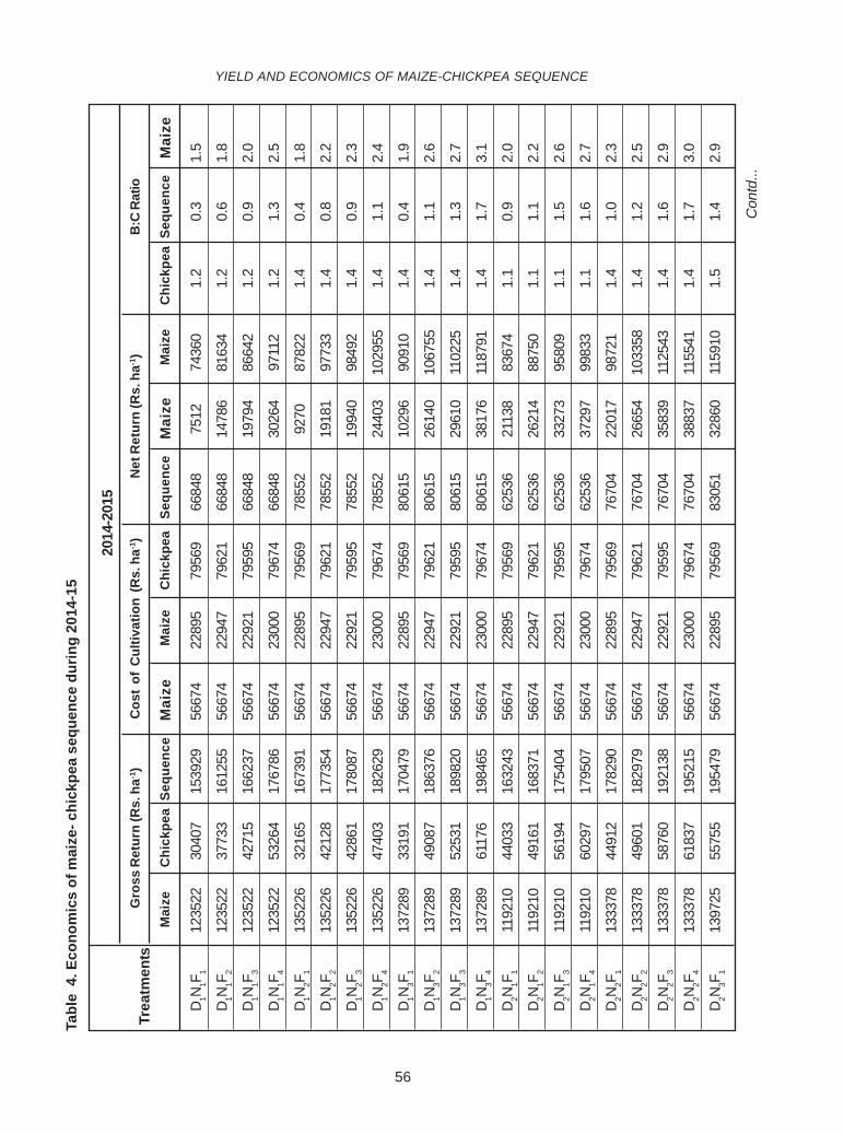
56
D1N
1F1
1235
2230
407
1539
2956
674
2289
579
569
6684
875
1274
360
1.2
0.3
1.5
D1N
1F2
1235
2237
733
1612
5556
674
2294
779
621
6684
814
786
8163
41.
20.
61.
8
D1N
1F3
1235
2242
715
1662
3756
674
2292
179
595
6684
819
794
8664
21.
20.
92.
0
D1N
1F4
1235
2253
264
1767
8656
674
2300
079
674
6684
830
264
9711
21.
21.
32.
5
D1N
2F1
1352
2632
165
1673
9156
674
2289
579
569
7855
292
7087
822
1.4
0.4
1.8
D1N
2F2
1352
2642
128
1773
5456
674
2294
779
621
7855
219
181
9773
31.
40.
82.
2
D1N
2F3
1352
2642
861
1780
8756
674
2292
179
595
7855
219
940
9849
21.
40.
92.
3
D1N
2F4
1352
2647
403
1826
2956
674
2300
079
674
7855
224
403
1029
551.
41.
12.
4
D1N
3F1
1372
8933
191
1704
7956
674
2289
579
569
8061
510
296
9091
01.
40.
41.
9
D1N
3F2
1372
8949
087
1863
7656
674
2294
779
621
8061
526
140
1067
551.
41.
12.
6
D1N
3F3
1372
8952
531
1898
2056
674
2292
179
595
8061
529
610
1102
251.
41.
32.
7
D1N
3F4
1372
8961
176
1984
6556
674
2300
079
674
8061
538
176
1187
911.
41.
73.
1
D2N
1F1
1192
1044
033
1632
4356
674
2289
579
569
6253
621
138
8367
41.
10.
92.
0
D2N
1F2
1192
1049
161
1683
7156
674
2294
779
621
6253
626
214
8875
01.
11.
12.
2
D2N
1F3
1192
1056
194
1754
0456
674
2292
179
595
6253
633
273
9580
91.
11.
52.
6
D2N
1F4
1192
1060
297
1795
0756
674
2300
079
674
6253
637
297
9983
31.
11.
62.
7
D2N
2F1
1333
7844
912
1782
9056
674
2289
579
569
7670
422
017
9872
11.
41.
02.
3
D2N
2F2
1333
7849
601
1829
7956
674
2294
779
621
7670
426
654
1033
581.
41.
22.
5
D2N
2F3
1333
7858
760
1921
3856
674
2292
179
595
7670
435
839
1125
431.
41.
62.
9
D2N
2F4
1333
7861
837
1952
1556
674
2300
079
674
7670
438
837
1155
411.
41.
73.
0
D2N
3F1
1397
2555
755
1954
7956
674
2289
579
569
8305
132
860
1159
101.
51.
42.
9
Tabl
e 4
. Eco
nom
ics
of m
aize
- chi
ckpe
a se
quen
ce d
urin
g 20
14-1
5
Trea
tmen
tsM
aize
Chi
ckpe
aSe
quen
ceM
aize
Gro
ss R
etur
n (R
s. h
a-1)
Cos
t of
Cul
tivat
ion
(Rs.
ha-1
)N
et R
etur
n (R
s. h
a-1)
B:C
Rat
io
Mai
zeC
hick
pea
Sequ
ence
Mai
zeM
aize
Chi
ckpe
aSe
quen
ceM
aize
2014
-201
5
Con
td...
YIELD AND ECONOMICS OF MAIZE-CHICKPEA SEQUENCE
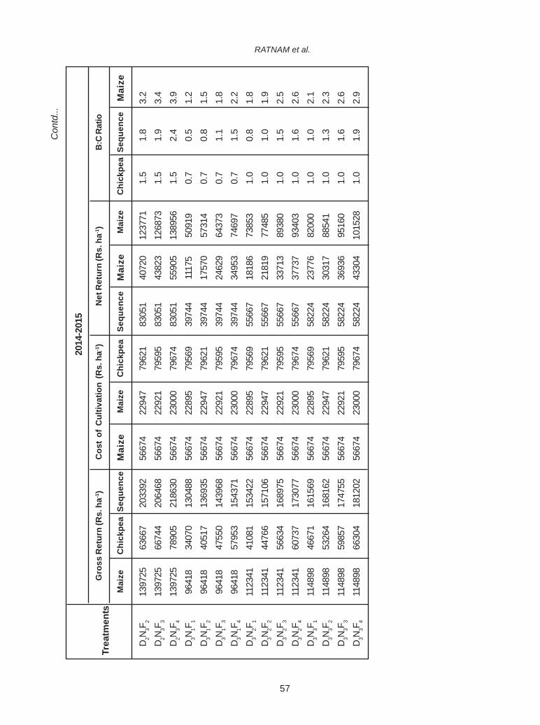
57
D2N
3F2
1397
2563
667
2033
9256
674
2294
779
621
8305
140
720
1237
711.
51.
83.
2D
2N3F
313
9725
6674
420
6468
5667
422
921
7959
583
051
4382
312
6873
1.5
1.9
3.4
D2N
3F4
1397
2578
905
2186
3056
674
2300
079
674
8305
155
905
1389
561.
52.
43.
9D
3N1F
196
418
3407
013
0488
5667
422
895
7956
939
744
1117
550
919
0.7
0.5
1.2
D3N
1F2
9641
840
517
1369
3556
674
2294
779
621
3974
417
570
5731
40.
70.
81.
5D
3N1F
396
418
4755
014
3968
5667
422
921
7959
539
744
2462
964
373
0.7
1.1
1.8
D3N
1F4
9641
857
953
1543
7156
674
2300
079
674
3974
434
953
7469
70.
71.
52.
2D
3N2F
111
2341
4108
115
3422
5667
422
895
7956
955
667
1818
673
853
1.0
0.8
1.8
D3N
2F2
1123
4144
766
1571
0656
674
2294
779
621
5566
721
819
7748
51.
01.
01.
9D
3N2F
311
2341
5663
416
8975
5667
422
921
7959
555
667
3371
389
380
1.0
1.5
2.5
D3N
2F4
1123
4160
737
1730
7756
674
2300
079
674
5566
737
737
9340
31.
01.
62.
6D
3N3F
111
4898
4667
116
1569
5667
422
895
7956
958
224
2377
682
000
1.0
1.0
2.1
D3N
3F2
1148
9853
264
1681
6256
674
2294
779
621
5822
430
317
8854
11.
01.
32.
3D
3N3F
311
4898
5985
717
4755
5667
422
921
7959
558
224
3693
695
160
1.0
1.6
2.6
D3N
3F4
1148
9866
304
1812
0256
674
2300
079
674
5822
443
304
1015
281.
01.
92.
9
Trea
tmen
tsM
aize
Chi
ckpe
aSe
quen
ceM
aize
Gro
ss R
etur
n (R
s. h
a-1)
Cos
t of
Cul
tivat
ion
(Rs.
ha-1
)N
et R
etur
n (R
s. h
a-1)
B:C
Rat
io
Mai
zeC
hick
pea
Sequ
ence
Mai
zeM
aize
Chi
ckpe
aSe
quen
ceM
aize
2014
-201
5
RATNAM et al.C
ontd
...

58
nitrogen levels and inoculation with PGPRs.Crop and Environment. 4 (1): 35-38.
Jnanesha, A.C and Alagundagi, S.C. 2012. Integratednutrient management practices in maize-chickpea sequence cropping under broadbed and furrow in model watershed-Dharwad. Karnataka Journal of AgriculturalSciences. 25(4):154-157.
Lingaraju, B. S., Parameshwarappa, U. K., Hulihalliand Basavaraju, B. 2010. Effect of organicson production and economic feasibility inmaize-chickpea sequence Indian Journal ofAgricultural Science. 44 (3): 211-215.
Maryam Jasemi, Fereshteh Darabi and RahimNaseri. 2013. Effect of planting date andnitrogen fertilizer application on grain yieldand yield components in maize (SC 704).American-Eurasian Journal of Agricultureand Environmental Science. 13(7): 914-919.
Mosha, K and Raghavaiah,V.R. 2003. Integratednutrient management in maize-groundnutsequence. PhD Thesis submitted toAcharya N.G Ranga Agricultural University,Hyderabad.
Mohankumar, R and Hiremath, S.M.2015. Residualeffect of maize hybrids, plant population andfertility levels on performance of chickpeain maize-chickpea sequence. KarnatakaJournal of Agricultural Sciences. 28 (4): 482-485.
Nawale, S. S., Pawar, A. D., Lambade, B. M andUgale, N.S. 2009. Yield maximization ofchickpea through Integrated NutrientManagement (INM) applied to sorghum-chickpea sequence under irrigatedconditions.Legume Research. 32(4): 282-285.
Prathyusha, C and Hemalatha, S. 2013. Yield andeconomics of speciality corn at various
levels of nitrogen application underpongamia + maize agrisilvi system.International Journal of Advanced Research.1 (6): 476-481.
Saini, S.S and Vinod Kumar.2001. Studies onmicrobial biomass and available nutrientsunder integrated nutrient management insorghum-chickpea sequence. PhD Thesissubmitted to Maharana Pratap Universityof Agriculture and Technology, Udaipur.
Sharma, A.R and Behera ,U.K. 2009. Recycling oflegume residues for nitrogen economy andhigher productivity in maize (Zea mays)-wheat (Triticum aestivum) cropping system.Nutrient Cycling in Agroecosystems. 83:197-210.
Sreerekha, M., Subbaiah, G., Veeraraghavaiah, R.,Ashokarani, Y and Prasunarani, P. 2015.Influence of rabi legumes and nitrogen levelson growth and yield of summer maize.Andhra Agricultural Journal. 62 (3): 518-522.
Thomas Abraham, Thenua, O.V.S and Shivakumar,B.G. 2010. Impact of levels of irrigation andfertility gradients on drymatter production,nutrient uptake and yield on chickpea (Cicerarietinum) intercropping system. LegumeResearch. 33 (1) : 10-16.
Vidyavathi, G. S., Dasogh, B., Babalad, N .S.,Hebsur, S. K., Gali, Patil S. G andAlagawadi, A.R. 2011. Influence of nutrientmanagement practices on crop responseand economic in different cropping systemsin vertisols. Karnataka Journal of AgriculturalSciences. 24 (4): 455-460.
Wasnik Vinod Kumar, Reddy, A. P.K and Sudhanshu,S. Kasbe. 2012. Performance of wintermaize (Zea mays L.) under different ratesof nitrogen and plant population in southernTelangana region. Crop Research. 44 (3):269-273.
YIELD AND ECONOMICS OF MAIZE-CHICKPEA SEQUENCE

59
INTRODUCTION
In India, municipal solid waste generatedduring 2011-12 was 1,27,486 tonnes per day (TPD),out of which, 89,334 TPD (70%) of MSW wascollected and 15,881 TPD (12.45%) was processedor treated. In Andhra Pradesh, in toto it was reportedas 11, 500 TPD out of which 4200 TPD was fromHyderabad alone. There was an increase by about2.7 times of that reported in 1999-2000 as per MoEFin 2012.
Greater Hyderabad Municipal Corporationproposed ‘Integrated Municipal Solid WasteManagement Project’ in Jawaharnagar village,Shameerpet mandal, Rangareddy district forenvironmental clearance. As of now, in the East Zone,there are about 1,77,874 households and of them,1,27,580 are covered by tricycles for collection ofmunicipal solid waste. Similarly, in the West Zone,of the 2,23,611 households, about 1,51,064 arecovered by tricycles. The proposed auto-tippers, aftercollecting garbage from door-to-door, will also goaround the localities to clean up open dumps. Thecapital here generates 3,800 metric tons of garbagea day, of which it has been now established that
EFFECT OF URBAN COMPOST APPLICATION TO SOIL ONGROUND WATER QUALITY
V. RAMBABU NAIK, P. PRABHU PRASADINI and V. SAILAJADepartment of Soil Science and Agricultural Chemistry, College of Agriculture,
Professor Jayashankar Telangana State Agricultural University, Rajendranagar, Hyderabad-500030
Date of Receipt: 18.2.2017 Date of Acceptance: 28.4.2017
ABSTRACTA laboratory soil column experiment was conducted to study threat of heavy metals addition to ground water when
urban compost was applied to soil as manure. The treatments imposed were : T1 - Control, T2 - Urban compost @ 20 t ha-1, T3 -Urban compost @ 40 t ha-1, T4 - T2 + FYM @ 10 t ha-1, T5 - T3 + FYM @ 10 t ha-1, T6 - T2+ Humic acid @ 20 kg ha-1, T7 - T3 + Humic acid@ 20 kg ha-1, T8 - T2 + Biochar @ 5 t ha-1 and T9 - T3 + Biochar @ 5 t ha-1. The leachates collected during nine leaching events withthree pore volumes of water were analysed for pH, EC, nitrates, COD and heavy metals. It was found that the treatments effectwas significant on all the parameters studied. NO3-N of leachates was more than 10 ppm in Urban compost + FYM treatments andwhen urban compost was added @ 40 t ha-1. Iron, Zinc and Cr were not detected in the leachates of any treatment. Mn wasrecorded in treatments where biochar was applied. Heavy metals namely Pb, Ni, Co and Cd were high with high dose of urbancompost more so in combinations of biochar, humic acid and FYM in descending order in case of Pb and Ni, and no specific trendin case of Co and Cd.
J.Res. ANGRAU 45(2) 59-63, 2017
about 3,200 metric tons is transported to the dumpyard. The urban compost is being added toagricultural land for both, waste disposal and toimprove soil fertility. Hence, an attempt was madeto study the impact of use of urban compost inagricultural soils on ground water quality.
MATERIAL AND METHODS
Leachate studies were conducted on soilcolumns to examine the transport of heavy metalsbeyond the depth of 45 cm in the Department ofEnvironmental Science and Technology, College ofAgriculture, Acharya N.G. Ranga AgriculturalUniversity (Presently PJTSAU )Rajendranagar in theyear 2012. Soil passed through 2 mm sieve waspacked in the column from bottom to top to a heightof 45 cm maintaining the bulk density of 1.6 Mg m-3.A space of 5 cm was provided at the top (above thesoil surface) for the application of water. Top 15 cmof the column was filled with 1/3rd of the calculatedquantity of soil mixed with urban compost (UC) with/without amendments as per the treatment. Thecolumns were mounted on plastic funnels providedwith plastic jar for collection of leachates. The
E-mail: [email protected]

60
treatments imposed were : T1 - Control, T2 - Urbancompost @ 20 t ha-1, T3 - Urban compost @ 40 tha-1, T4 -T2 + FYM @ 10 t ha-1, T5 - T3 + FYM @ 10 tha-1, T6 -T2 + Humic acid @ 20 kg ha-1, T7 -T3 + Humicacid @ 20 kg ha-1, T8 -T2 + Biochar @ 5 t ha-1 and T9
-T3 + Biochar @ 5 t ha-1.
Leachate study
The leaching study was carried out basedon pore volume. A pore volume is the volume of waterrequired to replace water in a certain volume ofsaturated porous media. Accordingly, one porevolume of each column prepared was equal to 1480ml of water. For every leaching event 493.3 ml waterwas used and nine leaching events were done (threepore volumes).
The columns were allowed to saturate for24 hours, then the first leachate was collected byadding 493.3 ml of water i.e., 1/3 pore volume.Similarly, after every 24 hours, leachates werecollected upto ninth leaching event. Accumulatedleachate was analyzed for pH, EC, nitrates,micronutrients (Fe, Mn, Zn and Cu), heavy metals(Pb, Ni, Co, Cd and Cr) and chemical oxygen demand(COD) following standard procedures of wateranalysis (Tandon, 1999). The water used for leachatestudies was with pH of 7.43, EC of 0.25 dS m-1,COD of 111.65 and NO3-N of 0.99 mg L-1. The recordedvalues of heavy metals were 0.013, 0.018, 0.019,0.138 and 0.309 ppm for Cu, Cd, Ni, Pb and Co,respectively. Iron, Mn, Zn and Cr were not detected.
The data obtained from the laboratory soilcolumn experiment was analysed in CompletelyRandomized Design with factorial and thesignificance was tested by ‘F’ test.
RESULTS AND DISCUSSION
In order to know the extent of leaching of heavymetals when urban compost was applied alone or incombination with farm yard manure/ humic acid/biochar to soil, accumulated leachates collectedduring nine leaching events were analysed (Table 1)and discussed hereunder.
Reaction (pH)
The pH of leachate from urban composttreatment application was on par with Control (soilalone). There was an increase in pH with the additionof FYM and Biochar (BC) over the respective basedosage of urban compost; however, no trend wasnoticed on humic acid (HA) addition along with urbancompost (Table 1). Application of Urban compost @20 t ha-1 did not affect the pH of the leachate but ahigher level of 40 t ha-1 increased the pH of leachate.Addition of FYM along with Urban compost (T4 andT5) increased pH of leachates compared to T2 (UC@ 20 t ha-1) and T3 (UC @ 40 t ha-1). FYM leads toacidification of the soil by the way of leaching ofexchangeable bases (Ca2+, Mg2+, Na+ and K+) intosoil solution and subsequently resulting in theirleaching. Rama Krishna (2008) also reported thesame. However, the pH was within the range suitablefor irrigation use (Tandon, 1999). In the treatmentsT8 (UC @ 20 t ha-1 + Biochar @ 5 t ha-1) and T9 (UC@ 40 t ha-1 + Biochar 5 t ha-1) the mean pH values(7.48, 7.54, respectively) were higher compared toT1 (control), which could be because of alkalinity ofthe biochar.
Electrical Conductivity
Electrical conductivity, an index of saltloading, was significantly influenced by the additionof organic sources. The mean value of EC of leachatessignificantly increased in all the treatments comparedto the control (Table 1). Among all the treatments,the leachate of the treatment T5 (UC @ 40 t ha-1 +FYM @ 10 t ha-1) recorded the highest value andlowest was recorded in T1 (control). Increase in ECvalues was very well correlated with the applicationof urban compost along with farm yard manure,humic acid and biochar in the form of differenttreatments. Significantly higher alkalinity of leachatefrom urban compost and FYM treated soil could bedue to the acid leaching of base components in tothe leachate. Higher EC of leachate from biocharapplied soil could be due to the reason that the saltsadded to soil through organic sources might getdissolved in water and leached down into leachates.However, the percent increase in EC was highest
RAMBABU NAIK et al.

61
Trea
tmen
tpH
ECCO
DNO
3-NM
nCu
Ni
PbCo
Cd
dS m
-1
mg
L-1
ppm
T 1 S
oil a
lone
7.43
2.51
211.
651.
00BD
L*0.
013
0.01
90.
138
0.30
90.
018
T 2U
C @
20
t ha--
17.
432.
6321
3.28
5.39
BDL
0.01
70.
020
0.14
80.
317
0.01
9
T 3U
C @
40
t ha-1
7.45
2.70
380.
6310
.09
BDL
0.01
60.
047
0.17
20.
242
0.01
4
T 4U
C @
20
t ha-1
+ F
YM
@ 1
0 t h
a-17.
612.
7627
2.34
13.0
9BD
L0.
017
0.06
40.
171
0.32
30.
021
T 5U
C @
40
t ha-1
+ F
YM
@ 1
0 t h
a-17.
603.
6431
5.00
14.9
4BD
L0.
019
0.10
80.
186
0.24
60.
016
T 6U
C @
20
t ha--
1 +
HA
@ 2
0 K
g ha
-17.
682.
9920
0.16
3.81
BDL
0.02
20.
166
0.26
10.
317
0.01
4
T 7U
C @
40
t ha-1
+ H
A@
20
Kg
ha-1
7.36
2.91
232.
724.
48BD
L0.
020
0.21
00.
343
0.27
80.
015
T 8U
C @
20
t ha--
1 +
BC
@ 5
t ha
-17.
482.
6321
6.57
5.09
1.63
00.
022
0.19
20.
334
0.35
60.
016
T 9U
C @
40
t ha-1
+ B
C @
5 t
ha-1
7.54
2.80
239.
542.
903.
590
0.02
30.
210
0.36
00.
321
0.02
0
CD
(5%
)0.
020
0.04
418
.582
1.57
50.
015
0.00
40.
018
0.01
10.
018
0.00
4
SE
M +
0.00
70.
015
6.20
60.
526
0.00
50.
001
0.00
60.
004
0.00
60.
001
Tabl
e 1.
Effe
ct o
f urb
an c
ompo
st a
pplic
atio
n to
soi
l on
leac
hate
s (m
ean
over
3 c
olum
ns)
UC
– U
rban
Com
post
; HA
- Hum
ic A
cid;
BC
- Bio
char
; *B
DL-
Bel
ow D
etec
tabl
e Li
mit
and
was
take
n as
zer
o fo
r sta
tistic
al a
naly
sis;
CO
D –
Che
mic
al O
xyge
n D
eman
d
EFFECT OF URBAN COMPOST APPLICATION ON GROUND WATER QUALITY

62
with FYM combination followed by humic acid andbiochar. Ananda et al. (2006) also reported anincrease in electrical conductivity due to theapplication of organic sources.
Chemical Oxygen Demand
COD was significantly influenced by differenttreatments of urban compost with FYM, humic acidand biochar. The increase in COD on application ofurban compost was non-significant when applied@ 20 t ha-1 and was significant when applied @ 40 tha-1 compared to Control. Shaheda Niloufer et al.(2013) also observed high COD values in the groundwater because of the leachate percolation from MSWlandfill. No specific trend was observed with theaddition of FYM/biochar component to urbancompost.With the conjunctive use of humic acid,COD values recorded were low compared toapplication of UC alone, which might be due to theinteraction of both urban compost and humic acid.
Nitrates (NO3-N)
Nitrates content was high when urbancompost was applied to soil compared to T1 (control)was high, but not significant when applied @ 20 tha-1. NO3-N of leachates was more than 10 ppm inUrban compost + FYM treatments and when urbancompost was added @ 40 t ha-1. In the treatmentsof T4 (UC @ 20 t ha-1+ FYM @ 10 t ha-1) and T5 (UC@ 40 t ha-1 + FYM @ 10 t ha-1) the mean NO3-Nvalues (13.09, 14.94 mg l-1) were higher comparedto T2. However, addition of humic acid (T6 and T7 ) andbiochar (T8 and T9) along with urban compostdecreased nitrates content in leachate which couldbe due to their interaction with urban compost. Theleachate quality with respect to NO3-N was‘moderate’ (5 to 30 mg l-1) as per Tandon (1999).Ground water contamination with nitrates leachedfrom MSW landfill sites in Chennai was observed byRaman and Narayanan (2008).
Heavy metals
Data on heavy metals content as given inTable 1 indicates the significant effect of treatments.
Iron, Zinc and Chromium
Iron, zinc and chromium were not detectedin the leachates of any treatment and in the waterused for the leachate study.
Manganese
Mn was not detected in leachates from thetreatments, T1 to T7 and in the water used for thestudy. But in treatments where biochar was added@ 5 t ha-1 (T8 and T9) Mn was recorded as 1.630 and3.590 ppm, respectively indicating that applicationof biochar increased the availability of Mn.Manganese content in leachates was higher thanirrigation water standards i.e., 0.2 ppm as per Tandon(1999) and ground water WHO standards whichshould be < 0.4 ppm (Musa et al., 2013).
Copper
Urban compost application, T2 (20 t ha-1) andT3 (40 t ha-1), recorded significantly higher values ofCu compared to control (T1), however, they werestatistically on par. This could be because of highercopper content in urban compost. The values werehigher with addition of FYM, humic acid and biocharin ascending order compared to T2 and T3.
Nickel
Ni content in leachates was found increasedwith successive addition of urban compost (T2 andT3) compared to T1 (control). Similarly, addition ofFYM, humic acid and biochar recorded higher Nivalues of leachates, compared to respective dosesof urban compost, T2 (UC @ 20 t ha-1) and T3 (UC @40 t ha-1). The leachate from soil column where urbancompost was applied @ 40t ha-1 along with humicacid or biochar were higher than the permissiblelimits of irrigation water (<0.2ppm as perTandon,1999) and ground water (<0.02 ppm as perWHO standards as reported by Musa et al., in 2013).The finding of possibility of contamination of groundwater by leaching of Ni was in accordance with thereports of Seyede (2013).
Lead
Application of urban compost @ 20 and 40 tha-1 resulted in significantly higher values of Pb inleachates over control. Similarly, inclusion of FYM@ 10 t ha-1, humic acid @ 20 kg ha-1 and biochar @5 t ha-1 to urban compost also resulted in significantlyhigher Pb content in leachates compared to
RAMBABU NAIK et al.

63
respective urban compost doses i.e., T2, UC @ 20 tha-1 and T3, UC @ 40 t ha-1. Lead limits were incompliance with standards of irrigation water i.e., <5 ppm as per Tandon (1999) and WHO ground waterstandard of max.0.4 ppm (Musa et al., 2013). Theleaching of lead from MSW dump sites into theground water was recorded by Effiong and Percy(2013).
Cobalt
Cobalt content varied significantly among thetreatments. In general, it was high with urban compostapplication @ 20 t ha-1 compared to control, but whileadding more urban compost to 40 t ha-1 recordedlow Co value (0.242 ppm). The same trend wasnoticed in treatment combinations of UC @ 40 tha-1 + FYM/humic acid/biochar compared to theirrespective combinations with UC @ 20 t ha-1
.
Cadmium
In general, Cd values in leachates werehigher than the permissible limit of max.0.003 ppmin ground water as per World Health Organization(Musa et al., 2013). Urban compost application @20 t ha-1 to soil resulted in slightly higher Cd contentin leachate compared to control. The leaching of Cdfrom MSW dump sites into the ground water wasrecorded by Effiong and Percy (2013). It was observedthat Biochar addition @ 5 t ha-1 could decrease theCd content in leachate when urban compost wasapplied in lower dose @ 20 ha-1 but was not effectivewith respect to Cd in leachate at higher dose of 40 tha-1. Whereas humic acid @ 20 kg ha-1 was effectivein reducing Cd content of leachates at both doses ofurban compost application.
CONCLUSION
Urban compost application to soil to 40 tha-1 (with similar quality as that used in the study)could be applied to soil with caution as there is apossibility of addition of lead and nickel to groundwater on continuous use over a period of time.
REFERENCES
Ananda, M.G., Ananda, M.R., Reddy, V.C andKumar, M.Y.A. 2006. Soil pH, electrical
conductivity and organic carbon content ofsoil as influenced by paddy-groundnutcropping system and different organicsources. Environment and Ecology (1):158-160.
Effiong, U.E and Percy, C.O. 2013. Leachate qualitycharacteristics: A case study of twoindustrial solid waste dump sites. Journalof Environmental Protection. 4: 984-988.
Musa, O.K., Shaibu, M.M and Kudamnya, E.A.2013. Heavy metal concentration in groundwater around Obajana and its Environs, Kogistate, North Central Nigeria. AmericanInternational Journal of ContemporaryResearch. 3 (8):170-177.
Rama Krishna, S.V.S.S. 2008. Mobility andaccumulation of nutrients and heavy metalsin soil by effective microbial (EM) compostapplication. M.Sc Thesis submitted toAcharya N. G. Ranga AgriculturalUniversity, Hyderabad.
Raman, N and Narayanan, D.S. 2008. Impact of solidwaste on ground water and soil qualitynearer to pallavaram solid waste landfill sitein Chennai. Rasayan Journal of Chemistry.1 (4): 828-836.
Seyede, B.K. 2013. Impact of municipal wasteleachate application on soil properties andaccumulation of heavy metals in wheat(Triticum aestivum L). International Journalof Scientific Research in EnvironmentalSciences (IJSRES). 1(1): 1-6.
Shaheda Niloufer, Swamy, A.V.V.S and SyamalaDevi, K. 2013. Ground water quality in thevicinity of municipal solid waste dump sitesin Vijayawada, A.P. International Journal ofEngineering and Science Research. 3 (8):419-425.
Tandon,H.L.S.1999. Methods of analysis of soils,plants, waters and fertilizers. FertilisersDevelopment and ConsultationOrganization, New Delhi. pp.143.
EFFECT OF URBAN COMPOST APPLICATION ON GROUND WATER QUALITY
64
INTRODUCTION
Maize (Zea mays L.) is one of the mostimportant crops among the cereals in the worldagricultural economy both as food and fodder crop.In India, during 2014-15 maize was cultivated in 9.2million ha with 24.17 million tonnes production, andwith a productivity of 2.56 t ha-1. In Andhra Pradesh,the crop is cultivated in an area of 0.99 mha with4.23 million tonnes production and 4257 kg ha-1
(AICRP on Maize, 2016). Among the several factors,most dominant factor responsible for the lower yieldsof maize are weeds, which competes with crop fornutrients, water, sunlight and space. Wide spacing,intensive use of inputs and initial slow growth of maizeare some of the factors responsible for increasedweed growth. With the discovery of syntheticherbicides in the early 1930s, there was a shift incontrol methods towards high input and target-oriented ones (Singh et al., 2003). Nowadays labourcomponent in agriculture is becoming scarce. Useof herbicides to manage weeds forms an excellentalternative to manual weeding. In India, till date onlypre-emergence application of atrazine /pendimethalin
WEED MANAGEMENT WITH PRE AND POST EMERGENCEHERBICIDES IN MAIZE
A. SUBBARAMI REDDY *, A. S. RAO, G. SUBBA RAO, T .C. M. NAIDU,A. LALITHA KUMARI AND N. TRIMURTHULU
Regional Agricultural Research Station,Acharya N.G. Ranga Agricultural University, Guntur-522 034
Date of Receipt: 16.2.2017 Date of Acceptance: 10.4.2017
ABSTRACTA field experiment was conducted at the Regional Agricultural Research Station, Guntur, Andhra Pradesh during rabi
season of 2013 and 2014 to evaluate the efficacy of pre emergence herbicides atrazine, pendimethalin and post-emergenceherbicides tembotrione and topramezone combinations against weed flora in maize. The experimental field was highly infestedwith Cynodon dactylon, Dactyloctenium aegyptium and Digitaria arvensis among grasses, Cyperus rotundus among sedges,Trianthema portulacastrum, Cleome viscosa, Euphorbia hirta and Phyllanthus niruri among broad leaf weeds. Lowest weeddensity and weed dry weight was recorded in application of atrazine@ 1.25 kg a.i ha-1 as pre-emergence followed by topramezone@ 25 g a.i ha-1 at 20 DAS as post-emergence (T6), pendimethalin @ 0.75 kg a.i ha-1 as pre-emergence followed by topramezone@ 25 g a.i ha-1 at 20 DAS as post-emergence (T8), atrazine@ 1.25 kg a.i ha-1 as pre-emergence followed by tembotrione@110 ga.i ha-1 at 20 DAS as post-emergence (T7) and pendimethalin @ 0.75 kg a.i ha-1 as pre-emergence followed by tembotrione@110g a.i ha-1 at 20 DAS as post-emergence (T9) where sequential application of herbicides at all stages of crop growth.
J.Res. ANGRAU 45(2) 64-74, 2017
E- mail: [email protected]; * Part of PhD thesis of author
has been widely recommended for the control ofweeds in maize. There is a need of post-emergenceherbicide usage for management of weeds whichoccur at 15-25 days of crop and offer severecompetition for growth resources, thereby loweringthe productivity of maize. Hence, it is proposed totest the new post emergence herbicides withoutresidual effect in maize has greater field applicability.In most farming systems, competition for N is themost important factor than that of for all other nutrientsand it is well known that large fraction of the millionsof tonnes of nutrients added to soils every year arenot taken up by crop plants, as up to 50% of addednitrogen and 0.4 to 90% of added phosphorus goingwaste from crop fields (Simpson et al., 2011). Thissituation can be alleviated by employing microbialinoculants, which are beneficial to soil andrhizobacteria capable of promoting plant growth whilereducing fertilizer inputs up to 50% without any yieldloss compared to fully fertilized controls (Hayat etal., 2010). Keeping all these in view, the presentinvestigation was proposed to evaluate different preand post emergence herbicides against mixed weed

65
complex in maize during rabi season of 2013 and2014.
MATERIAL AND METHODS
A field experiment was conducted at theRegional Agricultural Research Station, Guntur,during rabi season of 2013 and 2014 in split plotdesign with nine weed management treatments asmain plots and three fertilizer treatments as sub plotsand all the treatments replicated thrice. Details aregiven below:
Main plots
T1- Weedy check, T2- Atrazine@ 1.25 kg a.i ha-1 aspre-emergence, T3- Pendimethalin @ 0.75 kg a.iha-1 as pre-emergence ,T4- Topramezone @ 25 ga.i ha-1 at 20 DAS as post-emergence , T5-Tembotrione@110 g a.i ha-1 at 20 DAS as post-emergence, T6- Atrazine@ 1.25 kg a.i ha-1 as pre-emergence, fb Topramezone @ 25 g a.i ha-1 at 20DAS as post-emergence , T7- Atrazine@ 1.25 kga.i ha-1 as pre-emergence fb Tembotrione@110 ga.i ha-1 at 20 DAS as post-emergence, T8-Pendimethalin @ 0.75 kg a.i ha-1 as pre-emergence fb Topramezone @ 25 g a.i ha-1 at 20DAS as post-emergence , T9- Pendimethalin @0.75 kg a.i ha-1 as pre-emergence fbTembotrione@110 g a.i ha-1 at 20 DAS as post-emergence.
Sub-Plots
F1- 50% RDF+ bio consortium (Azospirillum (5 kgha-1) + phosphate solubilizing bacteria (5 kgha-1) + potash solubilizing bacteria (5 kg ha-1)+vasicular arbuscular mycorrhiza (12.5 kg ha-1)+ vermicompost (500 kg ha-1)
F2- 75% RDF+ bioconsortium (Azospirillum (5 kg ha-
1) + phosphate solubilizing bacteria (5 kg ha-1) +potash solubilizing bacteria (5 kg ha-1) + vasiculararbuscular mycorrhiza (12.5 kg ha-1) +vermicompost (500 kg ha-1) ; F3- 100% RDF
Maize crop variety pioneer 30 V 92 is usedfor the study in both the years in main plots of size9.6 m x 4.8 m and sub plots 4.8 m x 2.9 m.Herbicides were sprayed with Knapsack sprayer fittedwith flat fan nozzle. The different cultural practicesrecommended for maize crop were adopted duringthe crop growth period. Weed sampling was donerandomly by placing a 0.5 m x 0.5 m quadrate attwo different locations in the experimental unit toassess the weed flora at 30, 90 DAS and at harvestingstages. Dry weight of total weed species wasrecorded after drying and expressed in g m-2.
The original data on weed densities andweed weights were subjected to square roottransformation (Vx+0.5) before statistical analysis.The original values were given in parentheses.Statistical significance was tested by applying F-test at 0.05 level of probability and critical differences(CD) were calculated for those parameters, whichturned significant (P< =0.05) to compare the effectsof different treatments.
RESULTS AND DISCUSSION
Weed flora of the experimental plot duringthe course of investigation were collected, identifiedand presented in Table 1. There were fifteen speciesof weeds belonging to eleven different families. Theweed flora consisted of four different grassesbelonging to poaceae family with Cynodon dactylonwas predominant weed in the experimental field. Insedges only Cyperus rotundus was recorded whereas incase of dicots, ten weed species belonging tonine different families were observed. Of which,Trianthema portulacastrum, Cleome viscosa,Euphorbia hirta and Phyllanthus niruri were the majorweeds observed. Vanaja (2007) and Srividya et al.(2011) have reported the similar weed flora in theirexperiments conducted in black soils of Krishna Zoneof Andhra Pradesh.
All the weed management practicesinfluenced the weed density in maize in both the
SUBBARAMI REDDY et al.

66
years of study at all the stages of crop growth whencompared to weedy check. At 30 DAS (Table 2) allthe weed management practices were on par witheach other except atrazine@ 1.25 kg a.i ha-1 aspre-emergence (T2) and pendimethalin @ 0.75 kg a.iha-1 as pre-emergence (T3). The lowest total weeddensity (2.9 and 2.9 number m-2) was recorded inatrazine@ 1.25 kg a.i ha-1 as pre-emergence fbtopramezone @ 25 g a.i ha-1 at 20 DAS as post-emergence (T6) and was on par with T8 atrazine @1.25 kg a.i ha-1 as pre-emergence followed bytembotrione@110 g a.i ha-1 at 20 DAS as post-emergence (T7) and pendimethalin @ 0.75 kg a.iha-1 as pre-emergence followed by tembotrione@110g a.i ha-1 at 20 DAS as post-emergence (T9) withwhich it was at par., and significantly superior to restof the treatments. The reduced weed density in thesetreatments (T6 toT9) may be due to the fact that theweeds were controlled by sequential application attwo stages i.e., pre emergence and post emergenceat 20 DAS. Similar line of observations were reportedby Patel et al. (2006) and Malviya and Singh (2007).Significantly lower weed dry density was recordedin topramezone @ 25 g a.i ha-1 at 20 DAS as post-emergence (T4) and tembotrione@110 g a.i ha-1 at20 DAS as post-emergence (T5) treatments becauseof the post-emergence spray at 20 DAS whicheffectively controlled the weeds and resulted in lowweed density at 30 DAS. At 90 DAS (Table 3) andat harvest (Table 4) almost similar trend was noticedin both the years of study in which all the sequentialapplications were on par with each other. With regardto nutrient management treatments there is nosignificant difference among the treatments on weeddensity at all stages of crop growth. All the threenutrient practices (F1,F2 and F3)are on-par with eachother at 30 DAS, 90 DAS and maturity during boththe years of study.
Critical review of the data indicates thatsequential application of pre emergence herbicidesfollowed by post emergence application oftopramezone or tembotrione reduced the weed
density considerably and resulted in lowest weeddensity among these treatments. The betterperformance of sequential application might be dueto the effective control of weeds at critical stages.The present findings are in conformity with thefindings of Sreenivas and Satyanarayana (1994),Sinha et al. (2003) and Sonawane et al.(2014).Nutrient management practices did not showany impact on weed density at any stage of the cropand there was no interaction effect among thetreatments in both the years.
Total weed dry matter
Total weed dry matter was recorded at 30,90 DAS and at maturity during both the years ofinvestigation. At 30 DAS (Table 5) all herbicidaltreatments were significantly superior over weedycheck in both the years of studies. Significantly, thelowest weeds dry weight (2.9 and 3.3 g. m-2) of totalweeds was recorded in atrazine @ 1.25 kg a.i ha-1
as pre-emergence followed by topramezone @ 25 ga.i ha-1 at 20 DAS as post-emergence (T6) ascompared to all other treatments except, treatmentstopramezone @ 25 g a.i ha-1 at 20 DAS as post-emergence (T4), tembotrione @110 g a.i ha-1 at 20DAS as post-emergence (T5), pendimethalin @ 0.75kg a.i ha-1 as pre-emergence followed bytopramezone @ 25 g a.i ha-1 at 20 DAS as post-emergence (T8), atrazine @ 1.25 kg a.i ha-1 as pre-emergence followed by tembotrione@110 g a.i ha-1
at 20 DAS as post-emergence (T7) and pendimethalin@ 0.75 kg a.i ha-1 as pre-emergence followed bytembotrione@110 g a.i ha-1 at 20 DAS as post-emergence (T9) with which it was at par. This couldbe attributed to reduced weed competition in the initialstage and control of late emerged weeds bysequential spray which led to lower weeds densityand lower weed dry matter. Similar findings werereported by Patel et al. (2006) and Ahmed andsusheela (2012). Significantly lower weed dry weightwas recorded in topramezone @ 25 g a.i ha-1 at 20DAS as post-emergence (T4) and tembotrione@110g a.i ha-1 at 20 DAS as post-emergence (T5)
WEED MANAGEMENT IN MAIZE

67
treatments because of the post-emergence spray at20 DAS which effectively controlled the weeds andresulted in low weed dry weight at 30 DAS.Thehighest weed dry weight (12.7 and 13.4 gm-2,respectively) was recorded in weedy check duringboth the years of study. Similar trend was continuedat 90 DAS (Table 6) and at harvest (Table 7) alsoduring both the years of study.
All the nutrient treatments (F1, F2 andF3)are on-par with each other at 30 DAS,90 DASand maturity during both the years of study. There
was no significance among the nutrient managementtreatments in sub plots during the two years of studyand there was no interaction affect among thetreatments. An appraisal of the data indicated thatthe weed dry matter showed gradual increase uptoharvest even though the weed density declined after60 DAS. This may be because of accumulation ofmore dry matter in weeds which was due to lowercompetition among weeds for resources. It alsoindicated that nutrient levels did not influenced theweed dry matter at any stage of the crop growth.
Table 1. Weed flora of the experimental field
S.No Botanical Name Common Name FamilyI Grasses1 Cynodon dactylon Bermuda grass Poaceae
2 Dactyloctenium aegyptium Crow foot grass Poaceae
3 Digitaria sanguinalis Large crab grass Poaceae
4 Panicum repens Torpedo grass Poaceae
II Sedges
1 Cyperus rotundus Purple nutsedge Cyperaceae
III Broad leaf weeds1 Borreria hispida Button weed Rubiaceae2 Cleome viscosa Wild mustard Capparidaceae3 Commelina benghalensis Day flower Commelinaceae4 Euphorbia hirta Garden spurge Euphorbiaceae5 Phyllanthus niruri Stone breaker Euphorbiaceae6 Sida acuta Broom weed Malvaceae7 Trianthema portulacastrum Horse pursulane Aizoaceae8 Tribulus terrestris Puncture vine Zygophyllaceae9 Trichodesma indicum Indian borage Boraginaceae10 Tridax procumbense Mexican Daisy Compositae
SUBBARAMI REDDY et al.

68
T 1W
eedy
chec
k9.
2 (86
.3)
8.8 (
78.3
)9.
0 (8
2.0)
9.0 (
82.2
)9.
3 (87
.0)
8.9 (
80.3
)9.
1 (82
.0)
9.1 (
83.1
)T 2
Atra
zine@
1.25
kg ai
ha-1
as pr
e-em
erge
nce
4.9 (
24.3
)4.
8 (24
.0)
5.0 (
25.0
)4.
9 (24
.4)
4.8 (
23.0
)4.
8 (23
.0)
4.5 (
21.7
)4.
8 (22
.6)
T 3Pe
ndim
etha
lin @
0.75
kg ai
ha-1
as pr
e-em
erge
nce
5.1 (
27.3
)5.
4 (30
.7)
5.0 (
26.0
)5.
2 (28
.0)
5.7 (
32.3
)5.
5 (31
.0)
5.1 (
27.3
)5.
4 (30
.2)
T 4To
pram
ezon
e @ 25
g ai
ha-1 at
20 D
AS as
post-
emer
genc
e3.
9 (14
.7)
3.9 (
14.7
)3.
7 (13
.3)
3.8 (
14.2
)4.
1 (16
.7)
4.0 (
15.3
)3.
7 (13
.7)
3.9 (
15.2
)T 5
Tem
botri
one@
110 g
ai ha
-1 at
20 D
AS as
post-
emer
genc
e4.
1 (16
.0)
3.9 (
14.7
)4.
0 (15
.3)
4.0 (
15.3
)4.
2 (17
.3)
4.1 (
16.3
)3.
9 (14
.7)
4.1 (
16.1
)T 6
Atra
zine@
1.25
kg ai
ha-1
as pr
e-em
erge
nce f
bto
pram
ezon
e @ 25
g ai
ha-1 at
20 D
AS as
post-
emer
genc
e2.
9 (8.
0)2.
9 (7.
7)3.
0 (8.
3)2.
9 (8.
0)2.
8 (7.
7)2.
8 (7.
7)3.
0 (8.
7)2.
9 (8.
0)T 7
Atra
zine@
1.25
kg ai
ha-1
as pr
e-em
erge
nce f
bte
mbo
trion
e@11
0 gai
ha-1 at
20 D
ASas
post-
emer
genc
e3.
3 (10
.7)
3.5 (
11.7
)3.
3 (10
.3)
3.4 (
10.9
)3.
4 (11
.0)
3.3 (
10.7
)3.
4 (11
.3)
3.4 (
11.0
)T 8
Pend
imet
halin
@ 0
.75
kg a
i ha-1
aspr
e-em
erge
nce f
b top
ram
ezon
e @ 25
g ai
ha-1 at
20 D
AS as
post-
emer
genc
e3.
0 (9.
0)3.
0 (8.
7)3.
2 (9.
7)3.
1 (9.
1)3.
1 (9.
3)3.
0 (8.
3)3.
4 (11
.0)
3.1 (
9.6)
T 9Pe
ndim
etha
lin @
0.7
5 kg
ai h
a-1 as
pre-
emer
genc
e fb t
embo
trion
e@11
0 gai
ha-1 at
20 D
AS as
post-
emer
genc
e3.
5 (12
.0)
3.4 (
11.3
)3.
4 (11
.3)
3.5 (
11.6
)3.
7 (13
.0)
3.1 (
9.3)
3.7 (
13.3
)3.
5 (11
.9)
Mean
4.4 (
23.1
)4.
4 (22
.4)
4.4 (
22.4
)4.
6 (24
.1)
4.4 (
22.4
)4.
4 (22
.6)
Wee
d man
agem
ent p
racti
ces (
Main
)0.5
0.632
.70.4
1.227
.8Nu
trien
t leve
ls (S
ub)
0.1NS
11.7
0.1NS
10.8
Wee
d man
agem
ent p
ract
ices x
Nut
rient
leve
ls0.8
NS0.7
NS
Note
: Dat
a tra
nsfo
rmed
to “x
+0.5
tran
sfor
mat
ions
. Fig
ures
in pa
rent
hesis
are o
rigin
al va
lues
; RDF
: Rec
omm
ende
d dos
e of fe
rtiliz
ers;
MI: M
icrob
ial in
ocul
ant
Tabl
e 2.
Den
sity
of t
otal
wee
ds (N
o. m
-2) a
t 30
DA
S in
mai
ze a
s in
fluen
ced
by h
erbi
cide
s ap
plic
atio
n
Wee
d m
anag
emen
t pra
ctic
es (M
ain)
T. No.
2013
-14
2014
-15
Mea
nM
ean
Nut
rient
Lev
els
(Sub
)N
utrie
nt L
evel
s (S
ub)
F1F2
F3F1
F2F3
50%
RDF+
MI
75%
RDF+
MI
100%
RDF
50%
RDF+
MI
75%
RDF+
MI
100%
RDF
WEED MANAGEMENT IN MAIZE
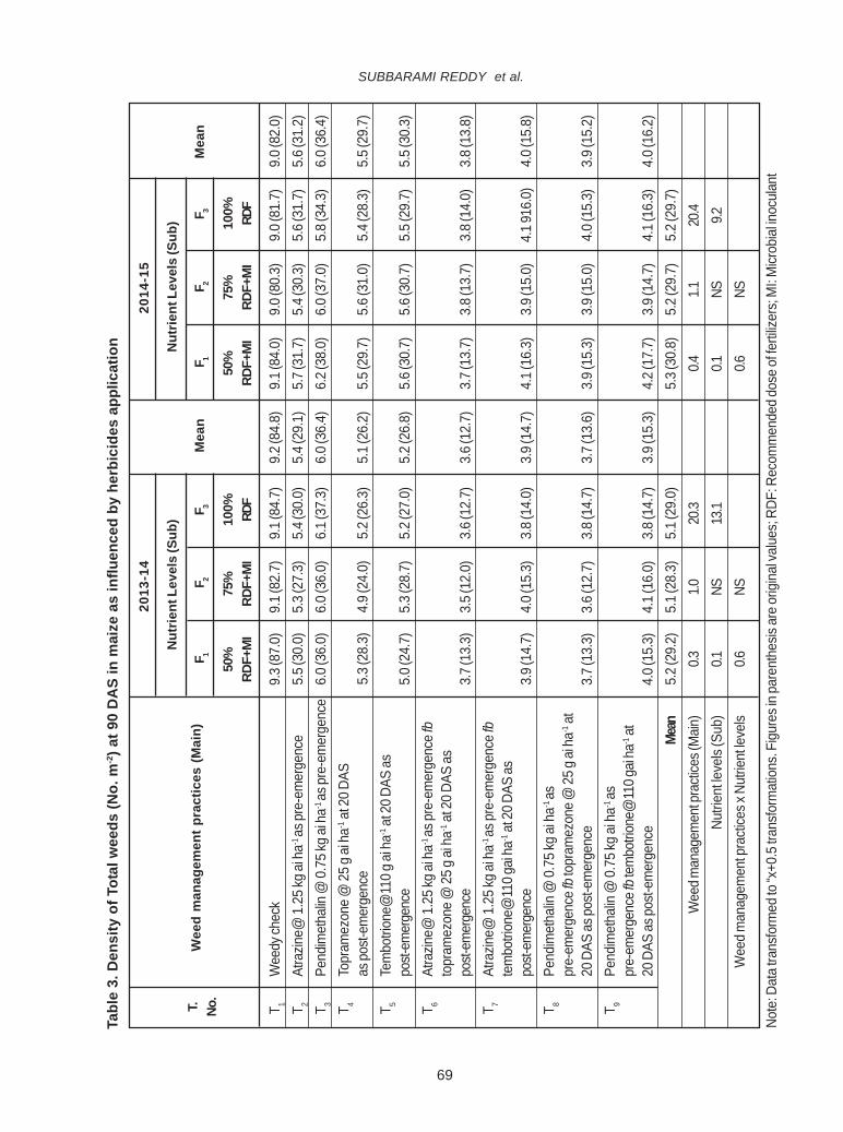
69
T 1W
eedy
chec
k9.
3 (87
.0)
9.1 (
82.7
)9.
1 (84
.7)
9.2 (
84.8
)9.
1 (84
.0)
9.0 (
80.3
)9.
0 (81
.7)
9.0 (
82.0
)T 2
Atra
zine@
1.25
kg ai
ha-1
as pr
e-em
erge
nce
5.5 (
30.0
)5.
3 (27
.3)
5.4 (
30.0
)5.
4 (29
.1)
5.7 (
31.7
)5.
4 (30
.3)
5.6 (
31.7
)5.
6 (31
.2)
T 3Pe
ndim
etha
lin @
0.75
kg ai
ha-1
as pr
e-em
erge
nce
6.0 (
36.0
)6.
0 (36
.0)
6.1 (
37.3
)6.
0 (36
.4)
6.2 (
38.0
)6.
0 (37
.0)
5.8 (
34.3
)6.
0 (36
.4)
T 4To
pram
ezon
e @ 25
g ai
ha-1 at
20 D
ASas
post-
emer
genc
e5.
3 (28
.3)
4.9 (
24.0
)5.
2 (26
.3)
5.1 (
26.2
)5.
5 (29
.7)
5.6 (
31.0
)5.
4 (28
.3)
5.5 (
29.7
)T 5
Tem
botri
one@
110 g
ai ha
-1 at
20 D
AS as
post-
emer
genc
e5.
0 (24
.7)
5.3 (
28.7
)5.
2 (27
.0)
5.2 (
26.8
)5.
6 (30
.7)
5.6 (
30.7
)5.
5 (29
.7)
5.5 (
30.3
)T 6
Atra
zine@
1.25
kg ai
ha-1
as pr
e-em
erge
nce f
bto
pram
ezon
e @ 25
g ai
ha-1 at
20 D
AS as
post-
emer
genc
e3.
7 (13
.3)
3.5 (
12.0
)3.
6 (12
.7)
3.6 (
12.7
)3.
7 (13
.7)
3.8 (
13.7
)3.
8 (14
.0)
3.8 (
13.8
)T 7
Atra
zine@
1.25
kg ai
ha-1
as pr
e-em
erge
nce f
bte
mbo
trion
e@11
0 gai
ha-1 at
20 D
AS as
post-
emer
genc
e3.
9 (14
.7)
4.0 (
15.3
)3.
8 (14
.0)
3.9 (
14.7
)4.
1 (16
.3)
3.9 (
15.0
)4.
1 916
.0)
4.0 (
15.8
)T 8
Pend
imet
halin
@ 0
.75
kg a
i ha-1
aspr
e-em
erge
nce f
b top
ram
ezon
e @ 25
g ai
ha-1 at
20 D
AS as
post-
emer
genc
e3.
7 (13
.3)
3.6 (
12.7
)3.
8 (14
.7)
3.7 (
13.6
)3.
9 (15
.3)
3.9 (
15.0
)4.
0 (15
.3)
3.9 (
15.2
)T 9
Pend
imet
halin
@ 0
.75
kg a
i ha-1
aspr
e-em
erge
nce f
b tem
botri
one@
110 g
ai ha
-1 at
20 D
AS as
post-
emer
genc
e4.
0 (15
.3)
4.1 (
16.0
)3.
8 (14
.7)
3.9 (
15.3
)4.
2 (17
.7)
3.9 (
14.7
)4.
1 (16
.3)
4.0 (
16.2
)Me
an5.
2 (29
.2)
5.1 (
28.3
)5.
1 (29
.0)
5.3 (
30.8
)5.
2 (29
.7)
5.2 (
29.7
)W
eed m
anag
emen
t pra
ctice
s (M
ain)
0.31.0
20.3
0.41.1
20.4
Nutri
ent le
vels
(Sub
)0.1
NS13
.10.1
NS9.2
Wee
d man
agem
ent p
ract
ices x
Nut
rient
leve
ls0.6
NS0.6
NS
Note
: Dat
a tra
nsfo
rmed
to “x
+0.5
tran
sfor
mat
ions
. Fig
ures
in pa
rent
hesis
are o
rigin
al va
lues
; RDF
: Rec
omm
ende
d dos
e of fe
rtiliz
ers;
MI: M
icrob
ial in
ocul
ant
Tabl
e 3.
Den
sity
of T
otal
wee
ds (N
o. m
-2) a
t 90
DA
S in
mai
ze a
s in
fluen
ced
by h
erbi
cide
s ap
plic
atio
n
Wee
d m
anag
emen
t pra
ctic
es (M
ain)
T. No.
2013
-14
Nut
rient
Lev
els
(Sub
)
F 1
50%
RDF+
MI
2014
-15
Mea
n
Nut
rient
Lev
els
(Sub
)
F 2F 3
F 1F 2
75%
RDF+
MI
100%
RDF
50%
RDF+
MI
75%
RDF+
MI
Mea
nF 3
100%
RDF
SUBBARAMI REDDY et al.

70
T 1W
eedy
chec
k8.
4 (70
.7)
8.2 (
66.3
)8.
3 (68
.0)
8.3 (
68.3
)8.
3 (69
.7)
8.2 (
67.3
)8.
0 (65
.0)
8.2 (
67.3
)T 2
Atra
zine@
1.25
kg ai
ha-1
as pr
e-em
erge
nce
4.6 (
20.7
)4.
3 (18
.3)
4.7 (
21.3
)4.
5 (20
.1)
4.9 (
23.3
)4.
7 (21
.3)
4.8 (
23.7
)4.
8 (22
.8)
T 3Pe
ndim
etha
lin @
0.75
kg ai
ha-1
as pr
e-em
erge
nce
5.0 (
25.0
)5.
2 (27
.3)
5.0 (
25.0
)5.
1 (25
.8)
5.1 (
26.3
)5.
2 (26
.7)
5.1 (
26.0
)5.
1 (26
.3)
T 4To
pram
ezon
e @ 25
g ai
ha-1 at
20DA
S as
post-
emer
genc
e4.
6 (20
.3)
4.5 (
18.0
)4.
4 (19
.3)
4.5 (
19.2
)4.
5 (20
.3)
4.5 (
22.3
)4.
5 (21
.3)
4.5 (
21.3
)T 5
Tem
botri
one@
110 g
ai ha
-1 at
20 D
AS as
post-
emer
genc
e4.
2 (17
.3)
4.5 (
20.0
)4.
7 (22
.0)
4.5 (
19.8
)4.
6 (20
.7)
4.6 (
20.7
)4.
6 (21
.3)
4.6 (
20.9
)T 6
Atra
zine@
1.25
kg ai
ha-1
as pr
e-em
erge
nce f
bto
pram
ezon
e @ 25
g ai
ha-1 at
20 D
AS as
post-
emer
genc
e2.
7 (7.
3)2.
6 (7.
0)2.
5 (7.
0)2.
6 (7.
1)2.
9 (8.
3)2.
9 (8.
3)2.
8 (8.
0)2.
9 (8.
2)T 7
Atra
zine@
1.25
kg ai
ha-1
as pr
e-em
erge
nce f
bte
mbo
trion
e@11
0 g ai
ha-1 at
20 D
AS as
post-
emer
genc
e2.
9 (8.
3)3.
1 (10
.0)
2.9 (
8.0)
3.0 (
8.8)
3.1 (
9.3)
3.0 (
8.7)
3.2 (
10.0
)3.
1 (9.
3)T 8
Pend
imet
halin
@ 0
.75
kg a
i ha-1
aspr
e-em
erge
nce f
b top
ram
ezon
e @ 25
g ai
ha-1 at
20 D
AS as
post-
emer
genc
e2.
8 (7.
3)2.
9 (8.
0)2.
8 (8.
3)2.
8 (7.
9)3.
0 (8.
7)3.
3 (10
.3)
2.8 (
8.0)
3.0 (
9.0)
T 9Pe
ndim
etha
lin @
0.7
5 kg
ai h
a-1 as
pre-
emer
genc
e fb t
embo
trion
e@11
0 g ai
ha-1 at
20 D
AS as
post-
emer
genc
e3.
1 (9.
3)3.
1 (9.
0)2.
9 (9.
0)3.
0 (9.
1)3.
2 (9.
7)3.
0 (9.
0)3.
3 (10
.7)
3.2 (
9.8)
Mean
4.2 (
20.7
)4.
3 (20
.4)
4.2 (
20.9
)4.
4 (21
.8)
4.4 (
21.6
)4.
4 (21
.6)
Wee
d man
agem
ent p
racti
ces (
Main
)0.3
0.818
.60.3
0.920
.3Nu
trien
t leve
ls (S
ub)
0.1NS
17.7
0.2NS
18.5
Wee
d man
agem
ent p
ract
ices x
Nut
rient
leve
ls0.5
NS0.5
NS
Note
: Dat
a tra
nsfo
rmed
to “x
+0.5
tran
sfor
mat
ions
. Fig
ures
in pa
rent
hesis
are o
rigin
al va
lues
; RDF
: Rec
omm
ende
d dos
e of fe
rtiliz
ers;
MI: M
icrob
ial in
ocul
ant
Tabl
e 4.
Den
sity
of t
otal
wee
ds (N
o. m
-2) a
t har
vest
in m
aize
as
influ
ence
d by
her
bici
des
appl
icat
ion
Wee
d m
anag
emen
t pra
ctic
es (M
ain)
T. No.
2013
-14
Nut
rient
Lev
els
(Sub
)
F 1
50%
RDF+
MI
2014
-15
Mea
nM
ean
Nut
rient
Lev
els
(Sub
)
F 2F 3
F 1F 2
F 3
75%
RDF+
MI
100%
RDF
50%
RDF+
MI
75%
RDF+
MI
100%
RDF
WEED MANAGEMENT IN MAIZE

71
T 1W
eedy
chec
k13
.1 (1
71.5
)12
.5 (1
56.4
)12
.7 (1
59.7
)12
.8 (1
62.5
)13
.6 (1
84.8
)13
.1 (1
73.1
)13
.6 (1
84.4
)13
.4 (1
80.8
)T 2
Atra
zine@
1.25
kg ai
ha-1
as pr
e-em
erge
nce
5.3 (
27.8
)5.
5 (31
.6)
5.2 (
26.8
)5.
3 (28
.7)
5.8 (
33.8
)5.
9 (34
.2)
5.7 (
32.0
)5.
8 (33
.3)
T 3Pe
ndim
etha
lin @
0.75
kg ai
ha-1
as pr
e-em
erge
nce
5.7 (
32.5
)5.
4 (28
.6)
5.4 (
28.3
)5.
5 (29
.8)
6.6 (
43.2
)5.
7 (31
.8)
5.7 (
32.5
)6.
0 (35
.8)
T 4To
pram
ezon
e @ 25
g ai
ha-1 at
20 D
ASas
post-
emer
genc
e3.
3 (10
.7)
3.8 (
14.3
)3.
5 (11
.8)
3.6 (
12.2
)3.
9 (14
.9)
3.9 (
16.1
)3.
9 (14
.9)
3.9 (
15.3
)T 5
Tem
botri
one@
110 g
ai ha
-1 at
20 D
ASas
post-
emer
genc
e3.
8 (14
.3)
4.0 (
16.1
)3.
5 (11
.6)
3.8 (
14.0
)3.
8 (14
.3)
4.0 (
15.7
)4.
3 (18
.3)
4.1 (
16.1
)T 6
Atra
zine@
1.25
kg ai
ha-1
as pr
e-em
erge
nce f
bto
pram
ezon
e @ 25
g ai
ha-1 at
20 D
ASas
post-
emer
genc
e2.
7 (6.
7)3.
0 (9.
0)2.
9 (8.
2)2.
9 (8.
0)3.
2 (9.
9)3.
3 (10
.7)
3.4 (
11.3
)3.
3 (10
.6)
T 7At
razin
e@ 1.
25 kg
ai ha
-1 as
pre-
emer
genc
e fb
tem
botri
one@
110 g
ai ha
-1 at
20 D
ASas
post-
emer
genc
e3.
2 (9.
5)3.
3 (10
.7)
3.2 (
10.1
)3.
2 (10
.1)
3.4 (
10.8
)3.
8 (13
.9)
3.7 (
13.6
)3.
6 (12
.8)
T 8Pe
ndim
etha
lin @
0.75
kg ai
ha-1
as pr
e-em
erge
nce f
b top
ram
ezon
e @ 25
g ai
ha-1
at 20
DAS
as po
st-e
mer
genc
e3.
0 (8.
5)3.
4 (11
.4)
2.9 (
8.1)
3.1 (
9.4)
3.2 (
10.1
)3.
4 (11
.2)
3.6 (
12.7
)3.
4 (11
.3)
T 9Pe
ndim
etha
lin @
0.75
kg ai
ha-1
as pr
e-em
erge
nce
fb te
mbo
trion
e@11
0 g ai
ha-1 at
20 D
ASas
post-
emer
genc
e3.
3 (10
.5)
3.5 (
12.0
)3.
2 (10
.0)
3.4 (
10.9
)3.
6 (12
.8)
3.5 (
12.1
)3.
6 (12
.8)
3.6 (
12.6
)Me
an4.
8 (32
.4)
4.9 (
32.2
)4.
7 (30
.5)
5.2 (
37.2
)5.
2 (35
.4)
5.3 (
36.9
)W
eed m
anag
emen
t pra
ctice
s (M
ain)
0.30.9
18.4
0.31.0
19.1
Nutri
ent le
vels
(Sub
)0.1
NS10
.80.1
NS12
.6W
eed m
anag
emen
t pra
ctice
s X N
utrie
nt le
vels
0.5NS
0.6NS
Note
: Dat
a tra
nsfo
rmed
to “x
+0.5
tran
sfor
mat
ions
. Fig
ures
in pa
rent
hesis
are o
rigin
al va
lues
; RDF
: Rec
omm
ende
d dos
e of fe
rtiliz
ers;
MI: M
icrob
ial in
ocul
ant
Tabl
e 5.
Dry
wei
ght o
f tot
al w
eeds
at 3
0 D
AS
(g m
-2) i
n m
aize
as
influ
ence
d by
her
bici
des
appl
icat
ion
Wee
d m
anag
emen
t pra
ctic
es (M
ain)
T. No.
2013
-14
Nut
rient
Lev
els
(Sub
)
F 1
50%
RDF+
MI
F 2
75%
RDF+
MI
2014
-15
Mea
nM
ean
Nut
rient
Lev
els
(Sub
)
F 3F 1
F 2F 3
100%
RDF
50%
RDF+
MI
75%
RDF+
MI
100%
RDF
SUBBARAMI REDDY et al.

72
T 1W
eedy
chec
k14
.3 (2
03)
13.4
(179
)13
.3 (1
76)
13.6
(186
)16
.5 (2
71)
15.8
(249
)15
.3 (2
39.0
)15
.8 (2
53)
T 2At
razin
e@ 1.
25 kg
ai ha
-1 as
pre-
emer
genc
e7.
6 (58
.3)
7.3 (
54.7
)7.
1 (52
.1)
7.3 (
55.0
)8.
1 (64
.8)
8.4 (
70.6
)7.
9 (63
.9)
8.1 (
66.4
)T 3
Pend
imet
halin
@ 0.
75 kg
ai ha
-1 as
pre-
emer
genc
e8.
3 (69
.5)
7.8 (
61.6
)9.
0 (80
.7)
8.4 (
70.6
)9.
2 (84
.2)
8.7 (
75.3
)8.
9 (79
.8)
8.9 (
79.7
)T 4
Topr
amez
one @
25 g
ai ha
-1 at
20 D
ASas
post-
emer
genc
e7.
3 (53
.1)
7.3 (
52.5
)7.
1 (51
.6)
7.2 (
52.4
)7.
4 (54
.0)
7.4 (
54.1
)7.
2 (52
.7)
7.3 (
53.6
)T 5
Tem
botri
one@
110 g
ai ha
-1 at
20 D
ASas
post-
emer
genc
e7.
7 (58
.6)
6.8 (
46.2
)7.
6 (57
.9)
7.4 (
54.2
)7.
7 (59
.9)
7.0 (
48.7
)7.
6 (58
.2)
7.4 (
55.6
)T 6
Atra
zine@
1.25
kg ai
ha-1
as pr
e-em
erge
nce f
bto
pram
ezon
e @ 25
g ai
ha-1 at
20 D
ASas
post-
emer
genc
e4.
8 (22
.9)
5.6 (
31.9
)4.
5 (19
.8)
5.0 (
24.9
)4.
8 (23
.4)
5.7 (
32.5
)4.
6 (20
.6)
5.0 (
25.5
)T 7
Atra
zine@
1.25
kg ai
ha-1
as pr
e-em
erge
nce f
bte
mbo
trion
e@11
0 g ai
ha-1 at
20 D
AS as
post-
emer
genc
e5.
1 (25
.3)
5.8 (
34.4
)5.
1 (26
.0)
5.3 (
28.6
)5.
1 (26
.2)
5.9 (
34.9
)5.
2 (27
.2)
5.4 (
29.4
)T 8
Pend
imet
halin
@ 0.
75 kg
ai ha
-1 as
pre-
emer
genc
efb
topr
amez
one @
25 g
ai ha
-1 at
20DA
S as
post-
emer
genc
e4.
8 (22
.6)
5.6 (
31.4
)4.
9 (24
.0)
5.1 (
26.0
)4.
9 (23
.4)
5.7 (
32.3
)5.
0 (24
.5)
5.2 (
26.7
)T 9
Pend
imet
halin
@ 0.
75 kg
ai ha
-1 as
pre-
emer
genc
efb
tem
botri
one@
110 g
ai ha
-1 at
20 D
ASas
post-
emer
genc
e5.
5 (29
.2)
6.0 (
35.2
)5.
3 (27
.5)
5.6 (
30.6
)5.
5 (29
.9)
6.0 (
36.5
)5.
3 (27
.7)
5.6 (
31.4
)Me
an7.
2 (60
.3)
7.3 (
58.6
)7.
1 (57
.3)
7.7 (
70.7
)7.
8 (70
.5)
7.4 (
66.0
)W
eed m
anag
emen
t pra
ctice
s (M
ain)
0.41.2
18.6
0.51.6
21.5
Nutri
ent le
vels
(Sub
)1.8
NS14
.30.2
NS10
.7W
eed m
anag
emen
t pra
ctice
s X N
utrie
nt le
vels
0.7NS
0.9NS
Note
: Dat
a tra
nsfo
rmed
to “x
+0.5
tran
sfor
mat
ions
. Fig
ures
in pa
rent
hesis
are o
rigin
al va
lues
; RDF
: Rec
omm
ende
d dos
e of fe
rtiliz
ers;
MI: M
icrob
ial in
ocul
ant
Tabl
e 6.
Dry
wei
ght o
f tot
al w
eeds
at 9
0 D
AS
(g m
-2) i
n m
aize
as
influ
ence
d by
her
bici
des
appl
icat
ion
Wee
d m
anag
emen
t pra
ctic
es (M
ain)
T. No.
2013
-14
Nut
rient
Lev
els
(Sub
)
F 1
50%
RDF+
MI
F 2
75%
RDF+
MI
2014
-15
Mea
nM
ean
Nut
rient
Lev
els
(Sub
)
F 3F 1
F 2F 3
100%
RDF
50%
RDF+
MI
75%
RDF+
MI
100%
RDF
WEED MANAGEMENT IN MAIZE
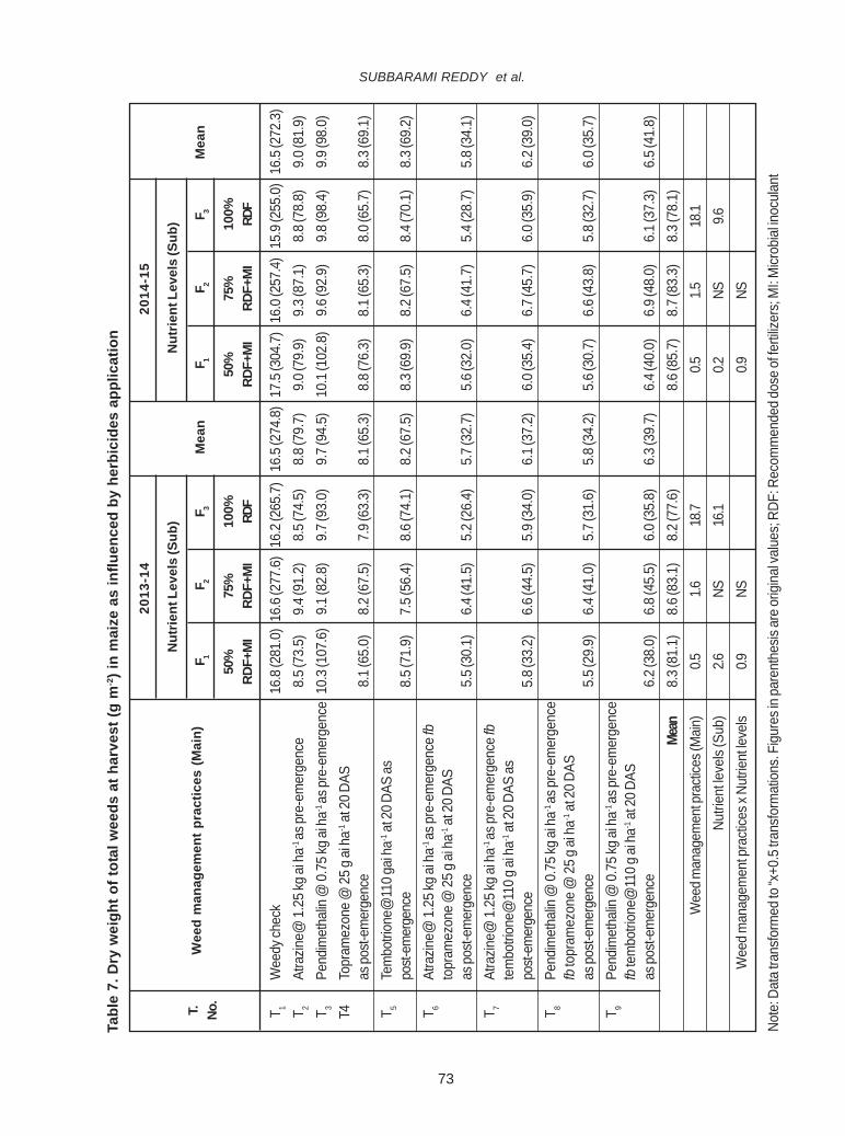
73
T 1W
eedy
chec
k16
.8 (2
81.0
)16
.6 (2
77.6
)16
.2 (2
65.7
)16
.5 (2
74.8
)17
.5 (3
04.7
)16
.0 (2
57.4
)15
.9 (2
55.0
)16
.5 (2
72.3
)T 2
Atra
zine@
1.25
kg ai
ha-1
as pr
e-em
erge
nce
8.5 (
73.5
)9.
4 (91
.2)
8.5 (
74.5
)8.
8 (79
.7)
9.0 (
79.9
)9.
3 (87
.1)
8.8 (
78.8
)9.
0 (81
.9)
T 3Pe
ndim
etha
lin @
0.75
kg ai
ha-1
as pr
e-em
erge
nce
10.3
(107
.6)
9.1 (
82.8
)9.
7 (93
.0)
9.7 (
94.5
)10
.1 (1
02.8
)9.
6 (92
.9)
9.8 (
98.4
)9.
9 (98
.0)
T4To
pram
ezon
e @ 25
g ai
ha-1 at
20 D
ASas
post-
emer
genc
e8.
1 (65
.0)
8.2 (
67.5
)7.
9 (63
.3)
8.1 (
65.3
)8.
8 (76
.3)
8.1 (
65.3
)8.
0 (65
.7)
8.3 (
69.1
)T 5
Tem
botri
one@
110 g
ai ha
-1 at
20 D
AS as
post-
emer
genc
e8.
5 (71
.9)
7.5 (
56.4
)8.
6 (74
.1)
8.2 (
67.5
)8.
3 (69
.9)
8.2 (
67.5
)8.
4 (70
.1)
8.3 (
69.2
)T 6
Atra
zine@
1.25
kg ai
ha-1
as pr
e-em
erge
nce f
bto
pram
ezon
e @ 25
g ai
ha-1 at
20 D
ASas
post-
emer
genc
e5.
5 (30
.1)
6.4 (
41.5
)5.
2 (26
.4)
5.7 (
32.7
)5.
6 (32
.0)
6.4 (
41.7
)5.
4 (28
.7)
5.8 (
34.1
)T 7
Atra
zine@
1.25
kg ai
ha-1
as pr
e-em
erge
nce f
bte
mbo
trion
e@11
0 g ai
ha-1 at
20 D
AS as
post-
emer
genc
e5.
8 (33
.2)
6.6 (
44.5
)5.
9 (34
.0)
6.1 (
37.2
)6.
0 (35
.4)
6.7 (
45.7
)6.
0 (35
.9)
6.2 (
39.0
)T 8
Pend
imet
halin
@ 0.
75 kg
ai ha
-1 as
pre-
emer
genc
efb
topr
amez
one
@ 2
5 g
ai h
a-1 at
20 D
ASas
post-
emer
genc
e5.
5 (29
.9)
6.4 (
41.0
)5.
7 (31
.6)
5.8 (
34.2
)5.
6 (30
.7)
6.6 (
43.8
)5.
8 (32
.7)
6.0 (
35.7
)T 9
Pend
imet
halin
@ 0.
75 kg
ai ha
-1 as
pre-
emer
genc
efb
tem
botri
one@
110 g
ai ha
-1 at
20 D
ASas
post-
emer
genc
e6.
2 (38
.0)
6.8 (
45.5
)6.
0 (35
.8)
6.3 (
39.7
)6.
4 (40
.0)
6.9 (
48.0
)6.
1 (37
.3)
6.5 (
41.8
)Me
an8.
3 (81
.1)
8.6 (
83.1
)8.
2 (77
.6)
8.6 (
85.7
)8.
7 (83
.3)
8.3 (
78.1
)W
eed m
anag
emen
t pra
ctice
s (M
ain)
0.51.6
18.7
0.51.5
18.1
Nutri
ent le
vels
(Sub
)2.6
NS16
.10.2
NS9.6
Wee
d man
agem
ent p
ract
ices x
Nut
rient
leve
ls0.9
NS0.9
NS
Note
: Dat
a tra
nsfo
rmed
to “x
+0.5
tran
sfor
mat
ions
. Fig
ures
in pa
rent
hesis
are o
rigin
al va
lues
; RDF
: Rec
omm
ende
d dos
e of fe
rtiliz
ers;
MI: M
icrob
ial in
ocul
ant
Tabl
e 7.
Dry
wei
ght o
f tot
al w
eeds
at h
arve
st (g
m-2) i
n m
aize
as
influ
ence
d by
her
bici
des
appl
icat
ion
Wee
d m
anag
emen
t pra
ctic
es (M
ain)
2013
-14
Nut
rient
Lev
els
(Sub
)
F 1
50%
RDF+
MI
F 2
75%
RDF+
MI
2014
-15
Mea
nM
ean
Nut
rient
Lev
els
(Sub
)
F 3F 1
F 2F 3
100%
RDF
50%
RDF+
MI
75%
RDF+
MI
100%
RDF
T. No.
SUBBARAMI REDDY et al.

74
CONCLUSION
Sequential application of herbicides i.e.,atrazine @ 1.25 kg a.i ha-1 as pre-emergence followedby topramezone @ 25 g a.i ha-1 at 20 DAS as post-emergence (T6) found to be superior and recordedlowest weed density and weed dry weight at allstages of crop growth. It can also be inferred thatnutrient levels have not shown any impact on weeddensity and weed dry weight at all stages of cropgrowth at any stage of crop growth. It was alsoconcluded that there is no interaction effect betweenweed management ant nutrient managementtreatments.
REFERENCES
Ahmed, A. M. A and Susheela, R. 2012. Weedmanagement studies in kharif maize. TheJournal of Research ANGRAU. 40 (3): 121-123.
All India Coordinated Research Project on Maize.2016. Trends in area, production andproductivity of maize. Annual MaizeWorkshop at University of AgriculturalSciences, Bangalore from 10-16 April,2016. Retrieved from the website (http://w w w . i i m r . r e s . i n / d o c u m e n t s /Directors%20Review%202016.pdf) on10.2.2017.
Hayat, R., Ali, S., Amara, V., Khalid, R and Ahmed,I. 2010. Soil beneficial bacteria and theirrole in plant growth promotion: A review.Annals of Microbiology. 60(4): 579-598.
Malviya, A and Singh, B. 2007. Weed dynamics,productivity and economics of maize (Zeamays L.) as affected by integrated weed
management under rainfed condition. IndianJournal of Agronomy. 52 (4): 321-324.
Patel, B.D., Chaudhari, D.D., Patel, V. J and Patel,R.B.2006. Pre- and post-emergenceherbicides for weed control in greengramand their residual effect on succeedingcrops. Indian Journal of Weed Science.48(1): 40–43.
Simpson, R.J., Oberson, A., Culvenor, R.A., Ryan,M.H., Veneklass, E.J and Lambers, H.2011.Strategies and agronomicinterventions to improve the phosphoroususe efficiency of farming systems. PlantSoil. 342 (1-2): 89-120.
Singh, H.P., Batish, D.R and Kohli, R.K. 2003.Allelopathic interactions and allelechemicals :new possibilities for sustainableweed management. Critical Reviews inPlant Sciences. 22:239-311.
Sonawane, R.K., Dandge, M.S., Kambel, A.S andShingrup, P.V. 2014. Effect of herbicideson nutrient uptake by weeds, crops andyield of kharif maize. Biennial Conferenceof Indian Society of Weed Science. pp.95.
Sreenivas, G and Satyanarayana, V. 1994. Integratedweed management in rainy season maize.Indian Journal of Agronomy. 39 (1): 166-167.
Srividya, S., Chandrasekhar, K and Veeraraghavaiah,R. 2011. Effect of tillage and herbicide useon weed management in maize. The AndhraAgricultural Journal. 58 (2): 123-126.
Vanaja, C.H. 2007.Weed management studies inkharif maize. M.Sc Thesis submitted toAcharya N.G. Ranga Agricultural University,Rajendranagar, Hyderabad.
WEED MANAGEMENT IN MAIZE

75
INTRODUCTION
Market intelligence is an essential functionfor the formulation of a sound price and trade policy,and its successful implementation. It serves as amechanism for understanding the behavior of relevantfactors; and helps in the evolution of a proper pricingpolicy and generating outlook information. Marketinformation creates competitive market process andchecks the growth of monopoly or profiteering byindividuals. It is the lifeblood of a market, becauseeveryone engaged in production, and in buying andselling of products is continually in need of marketinformation. This is true where agriculturalcommodities are concerned, because their pricesfluctuate more widely than those products of othersectors. The research in agricultural marketing insub-Saharan Africa, particularly of applied nature, hasbeen meagre and scanty because of the strenuousand time consuming job of collecting and maintaininga credible data from different market functionaries,because in most cases market functionaries are notready to part with correct information and data, thus,
GENERATING MARKET INFORMATION AND MARKET OUTLOOK OF MAJORCASSAVA MARKETS IN AFRICA: A DIRECTION FOR NIGERIA TRADE
INVESTMENT AND POLICYM. S. SADIQ, I. P SINGH, I.J. GREMA, S.M. UMAR AND M.A. ISAH
Department of Agricultural Economics,Swami Keshwanand Rajasthan Agricultural University, Bikaner – 334 006
Date of Receipt: 07.3.2017 Date of Acceptance: 02.5.2017
ABSTRACTThe findings confirmed the presence of cointegration, implying long-run price association among the related markets.
For additional evidence as to whether and in which direction price transmission was occurring between the markets pair, Grangercausality test indicated four unidirectional causalities: Rwanda-Nigeria; Ghana-Rwanda; Nigeria-Madagascar and Madagascar-Rwanda, while the remaining market pairs showed no causal relation between them. The impulse response functions conductedconfirmed the result of cointegration, but the magnitude of price transmission was found relatively low in some market pairs thatwere spatially integrated. Further, the findings indicated usefulness of cassava trading in the major cassava markets in Africagiven that explosive volatility pattern was not observed. ARIMA model could be used successfully for modeling as well asforecasting of yearly prices of cassava in the major markets in Africa given its good performance in terms of explained variabilityand predicting power. Based on findings, network design for major cassava markets across Africa at almost equal distance fromeach other to enhance market integration and better price transmission among them was recommended. Also, the high degree ofmarket integration observed in this case indicate that the major cassava markets in Africa were quite competitive, thus, providinglittle justification for extensive and costly intervention designed to enhance market efficiency via improved competition.
E-mail: [email protected]
J.Res. ANGRAU 45(2) 75-82, 2017
making marketing research in sub-Saharan Africanot to make headway for long, as such, a lot of scopeexists for research in this field. Therefore, there isan urgent need for an analysis of the most relevantvariables in marketing research. This research looksinto the perspective of cassava marketing in sub-Saharan Africa considering its nascent stage.Examples of studies on cassava marketing are Ibanaet al.(2009); Ijiako et al.(2013); Kwasi and Kobina(2014), and Ospina-Patino and Ezedinma (2015), butthe major drawback is that all these studies focusedon domestic marketing of this product; with noevidence based studies on international trade outlookof this commodity despite its emerging marketpotentials in the world. It is a known fact that theneed for research in cassava marketing has beenrecognized by the planners and policy makers, giventhat, research in this aspect can contribute to theestablishment of facts and evolution of the policymeasures that may be necessary for developing asuccessful marketing strategy with respect toproduction, consumption, distribution and pricing. A

76
smooth functioning of the marketing system isessential for price stability and for proper incentivesto the producers. In the present context, whenagricultural production is on the increase, themarketing system should be suitably altered tosustain the increase by providing efficient and promptservices. This can be achieved by keeping a constantwatch on developments and by anticipating theproblems in marketing of this commodity. Marketinformation is essential for the government, forcreating a policy environment for a smooth conductof the marketing business, and for the protection ofall the groups of persons associated with this. Also,it is essential at all the stages of marketing, fromthe sale of the produce at the farm until the goodsreach the last/final consumer.
MATERIAL AND METHODS
Africa is a continent comprising 63 politicalterritories, representing the largest of the greatsouthward projections from the main mass of Earth’ssurface. Yearly data on producer cassava prices ($/tons) in Ghana, Nigeria, Madagascar and Rwandamarkets spanning from 1991 to 2014 were sourcedfrom the FAOSTAT databank. Analytical techniquesused are described below:
Empirical Models
1. Model Selection Criteria
The information criteria are computed for the VARmodels of the form:
Yt = A1Yt-1 + ….. + AnYt-n + Bq Xt + …….. + BqXt-q
+ CDt + ……………………. (1)
Where Yt is K-dimensional. The lag order of theexogenous variables Xt, q, and deterministic term Dt
have to be pre-specified. For a range of lag orders nthe model is estimated by OLS. The optimal lag ischosen by minimizing one of the following informationcriteria:
AIC (n) = log det { } + (2/T) nK2 ….. (2)
HQ (n) = log det { } + (2log log T/T) nK2 ...(3)
SC (n) = log det { } + (log T/T) nK2 … (4)
FPE (n) = (T + n*/T-n*)k det { } .. (5)
Where { } is estimated by T-1 UtU1t, n*
is the total number of parameters in each equationof the model when n is the lag order of theendogenous variables, also counting the deterministicterms and exogenous variables. The sample lengthis the same for all different lag lengths and isdetermined by the maximum lag order.
2. Augmented Dickey Fuller Test
The Augmented Dickey-Fuller test (ADF) is the testfor the unit root in a time series sample (Blay et al.,2015). The autoregressive formulation of the ADF testwith a trend term is given below:
......… (6)
Where, pit is the price in market i at the time t, pit
(pit – pt-1) and is the intercept or trend term. Thejoint hypothesis to check the presence of unit rootis: statistic. Failure of therejection of null hypothesis means that the series isnon-stationary.
3. Johansen’s Co-integration Test
The Johansen procedure is a multivariategeneralization of the Dickey-Fuller test and theformulation is as follows (Johansen, 1988):
pt = A1 pt-1 + ……………………. (7)
So that
pt = A1 pt-1 – pt-1 + ………………… (8)
pt = (A1- I) pt-1 + ………………………. (9)
pt = + …………………………..... (10)
Where, pt and are (n×1) vectors; At is an (n x n)matrix of parameters; I is an (n x n) identity matrix;
and is the (At-1) matrix. The rank of (At -1) matrix
equals the number of co-integrating vectors. Thecrucial thing to check is whether (At-1) consists of all
SADIQ et al.

77
zeroes or not. If it does, then it implies that all the{pt} in the above VAR are unit root processes, andthere is one linear combination of which is stationary,and hence the variables are not co-integrated. Therank of matrix is equal to the number ofindependent co-integrating vectors. Both trace andmax test were used to determine the presence ofco-integrating relationship among and between theprice series. Using the estimates of the characteristicroots, the tests for the number of characteristic rootsthat are insignificantly different from unity wereconducted using the following statistics:
…….. (11)
…………………… (12)
Where, denotes the estimated values of thecharacteristic roots (eigen values) obtained from the
estimated matrix; and T is the number of usable
observations.
4. Granger Causality Test
Granger (1969) causality test was used to determinethe order and direction of short-term and long-termequilibrium relationships. Whether market p1 Grangercauses market p2 or vice-versa was checked usingthe following model:
,...… (13)
A simple test of the joint significance of wasused to check the Granger causality, i.e.
5. Vector Error Correction Model (VECM)
After establishing the multiple co-integratingrelationships among price series, Vector ErrorCorrection Model (VECM) was constructed todetermine the short-term disturbances and theadjustment mechanism to estimate the speed ofadjustment. The VECM explains the difference
and it is shown below:
…. (14)
It includes the lagged differences in both x and y,which have a more immediate impact on the value of
. For example, if increases by one
percentage point, then would increase by
percentage point. The value of indicates thepercentage point would change in the long-run inresponse to changes in x. Therefore, part of thechange in could be explained by y correctingitself in each period to ultimately reach the long-runpath with x. The amount by which the value of ychanges (or corrected) in each period is signified by
. This coefficient ( ) indicates the percentageof the remaining amount that y has to move to returnto its long- run path with x. In explaining changes ina variable, the VECM accounts for its long-runrelationship with other variables. The advantage ofVECM over an ordinary OLS model is that it accountsfor dynamic relationships that may exist between adependent variable and explanatory variable, whichmay span over several periods.
6. Impulse Response Functions
Granger causality tests do not determine the relativestrength of causality effects beyond the selected timespan. In such circumstances, causality tests areinappropriate because these tests are unable toindicate how much feedback exists from one variableto the other beyond the selected sample period(Rahman and Shahbaz, 2013; Beag and Singla,2014). The best way to interpret the implications ofthe models for patterns of price transmission,causality and adjustment are to consider the timepaths of prices after exogenous shocks, i.e. impulseresponses (Beag and Singla, 2014). The impulseresponse function traces the effect of one standarddeviation or one unit shock to one of the variables oncurrent and future values of all the endogenousvariables in a system over various time horizons
MARKET INFORMATION AND MARKET OUTLOOK OF CASSAVA MARKETS IN AFRICA

78
(Sadiq et al., 2016). For this study the generalizedimpulse response function (GIRF) originallydeveloped by Koop et al. (1996) and suggested byPesaran and Shin (1998) was used. The GIRF in thecase of an arbitrary current shock, and history,
is specified below:
........(15)
For n = 0, 1
7. GARCH Model
The representation of the GARCH (p, q) is given as:
(Autoregressive process) …………………. (16)
And the variance of random error is:
Where, Yt is the price in the ith period of the ith marketp is the order of the GARCH term and q is the order
of the ARCH term. The sum of gives the
degree of persistence of volatility in the series. Thecloser is the sum to 1; the greater is the tendency ofvolatility to persist for a longer time. If the sumexceeds 1, it is indicative of an explosive series witha tendency to meander away from the mean value.
8. ARIMA Model
A generalization of ARMA models which incorporatesa wide class of non-stationary time-series is obtainedby introducing the differencing into the model. Thesimplest example of a non-stationary process whichreduces to a stationary one after differencing is
Random Walk. A process is said to follow an
integrated ARMA model, denoted by ARIMA
is ARMA (p, q), and
the model is written below:
…….(19)
Where, and WN indicates white
noise. The integration parameter d is a non-negativeinteger. When d = 0, ARIMA (p, d, q) = ARMA (p, q).
Forecasting Accuracy
For measuring the accuracy in fitted time seriesmodel, mean absolute prediction error (MAPE),relative mean square prediction error (RMSPE) andrelative mean absolute prediction error (RMAPE) werecomputed using the following formulae (Paul, 2014):
MAPE = 1/T ……. (20)
RMPSE = 1/T ….. (21)
RMAPE = 1/T X 100 … (22)
Where, At = Actual value; Ft = Future value, and T=Time period(s)
RESULTS AND DISCUSSION
Summary statistics of yearly producer prices ofcassava in major cassava markets in Africa
The summary statistics of yearly prices ofcassava spanning from 1991 to 2014 are presentedin Table 1. The perusal of Table 1 reveals that theminimum values of the average prices varied from$38.96 per ton in Ghana market to $120.77 per tonin Nigeria market, while the maximum values of theaverage prices varied from $200.00 per ton inMadagascar market to $541.90 per ton in Nigeriamarket during the period under consideration. Theaverage prices per ton were found to be $111.99 inGhana market, $219.78 in Nigeria market, $130.13in Madagascar market and $228.30 in Rwandamarket. The standard deviation in prices was foundto be minimum in Madagascar market ($40.99 perton) and maximum in Nigeria market ($122.70 perton) during the period under consideration. Slightinstability in cassava prices were noticed in all theselected markets, with it being highest in Nigeriamarket during the period under consideration, whichmight be due to fluctuation in arrivals as a result ofseasonality. All the selected markets exhibitedpositively skewed distribution in their respective
SADIQ et al.

79
prices from year 1991 to 2014. Almost all the selectedmarkets showed a platykurtic (fat or short-tailed)probability distribution function except Nigeria market
which showed a leptokurtic (slim or long-tailed)pattern of distribution for the entire period underconsideration.
Table 1. Summary statistics of yearly producer prices of cassava in major cassava markets in Africa ($ per ton)
Market Min Max Mean STD CV Skewness Kurtosis IQ range
Ghana 38.96 210.00 111.99 50.71 0.45 0.36 -1.02 82.94
Nigeria 120.77 541.90 219.78 122.70 0.55 1.83 1.96 63.79
Madagascar 65.41 200.00 130.13 40.99 0.31 0.13 -1.28 74.12
Rwanda 79.78 368.81 228.30 87.12 0.38 0.011 -1.29 158.43
Lag Selection Criteria
Because of sensitivity of time series to laglength and to ensure that errors are white noise inADF, the information criteria viz., Akaike informationcriterion (AIC), Hannan–Quinn criterion (HQC) andSchwarz Bayesian criterion (BIC) were used toselect appropriate lag length for the analyses. Thetest results as shown in Table 2 reveal that the
optimum lag length appropriate for the specifiedvariables is lag 2 as indicated by the asterisks amongthe information criteria. This means that the optimumlag length for the series should be lag 2 in order toobtain more interpretable parsimonious models.However, it should be noted that when all theselection criteria agree, the selection is clear, but ina situation of conflicting results, the selection criteriawith the highest lag order is considered.
Table 2. Lag selection criteria
Lag(s) AIC BIC HQC
1 41.06 42.05 41.29
2 40.67* 42.45* 41.09*
Unit Root Test
To investigate the market integration,Augmented Dickey Fuller (ADF) test for unit root testwas conducted and the results shown in Table 3.The ADF values of all the series were non-significantat 5 per cent level of significance, indicating theexistence of unit root in the series; implying non-stationary nature of the data, but at first differencelevel, the ADF values for all the series were significantat 5 percent level of significance, implying that theseprice series were free from the consequences of unitroot; meaning that the price series were stationary
at first difference. ADF-GLS test, which provides analternate method for correcting serial correlation andheteroscedasticity, was used to validate the results.The results of the unit root test did not reject the nullhypothesis of presence of unit root when the serieswere considered at level. The first differenced serieswere found to be stationary, i.e., these are integratedof order one. Having ensured I(1) of the price series,the relationship between these markets wasestimated using the co-integration test; theconformation that each level series is I(1) allowed toproceed for Johansen’s cointegration test.
MARKET INFORMATION AND MARKET OUTLOOK OF CASSAVA MARKETS IN AFRICA
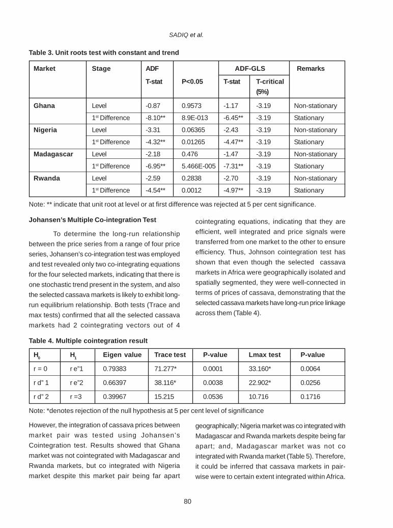
80
Table 3. Unit roots test with constant and trend
Market Stage ADF ADF-GLS Remarks
T-stat P<0.05 T-stat T-critical(5%)
Ghana Level -0.87 0.9573 -1.17 -3.19 Non-stationary
1st Difference -8.10** 8.9E-013 -6.45** -3.19 Stationary
Nigeria Level -3.31 0.06365 -2.43 -3.19 Non-stationary
1st Difference -4.32** 0.01265 -4.47** -3.19 Stationary
Madagascar Level -2.18 0.476 -1.47 -3.19 Non-stationary
1st Difference -6.95** 5.466E-005 -7.31** -3.19 Stationary
Rwanda Level -2.59 0.2838 -2.70 -3.19 Non-stationary
1st Difference -4.54** 0.0012 -4.97** -3.19 Stationary
Note: ** indicate that unit root at level or at first difference was rejected at 5 per cent significance.
Johansen’s Multiple Co-integration Test
To determine the long-run relationshipbetween the price series from a range of four priceseries, Johansen’s co-integration test was employedand test revealed only two co-integrating equationsfor the four selected markets, indicating that there isone stochastic trend present in the system, and alsothe selected cassava markets is likely to exhibit long-run equilibrium relationship. Both tests (Trace andmax tests) confirmed that all the selected cassavamarkets had 2 cointegrating vectors out of 4
cointegrating equations, indicating that they areefficient, well integrated and price signals weretransferred from one market to the other to ensureefficiency. Thus, Johnson cointegration test hasshown that even though the selected cassavamarkets in Africa were geographically isolated andspatially segmented, they were well-connected interms of prices of cassava, demonstrating that theselected cassava markets have long-run price linkageacross them (Table 4).
Table 4. Multiple cointegration result
H0 H1 Eigen value Trace test P-value Lmax test P-value
r = 0 r e”1 0.79383 71.277* 0.0001 33.160* 0.0064
r d” 1 r e”2 0.66397 38.116* 0.0038 22.902* 0.0256
r d” 2 r =3 0.39967 15.215 0.0536 10.716 0.1716
Note: *denotes rejection of the null hypothesis at 5 per cent level of significance
However, the integration of cassava prices betweenmarket pair was tested using Johansen’sCointegration test. Results showed that Ghanamarket was not cointegrated with Madagascar andRwanda markets, but co integrated with Nigeriamarket despite this market pair being far apart
geographically; Nigeria market was co integrated withMadagascar and Rwanda markets despite being farapart; and, Madagascar market was not cointegrated with Rwanda market (Table 5). Therefore,it could be inferred that cassava markets in pair-wise were to certain extent integrated within Africa.
SADIQ et al.
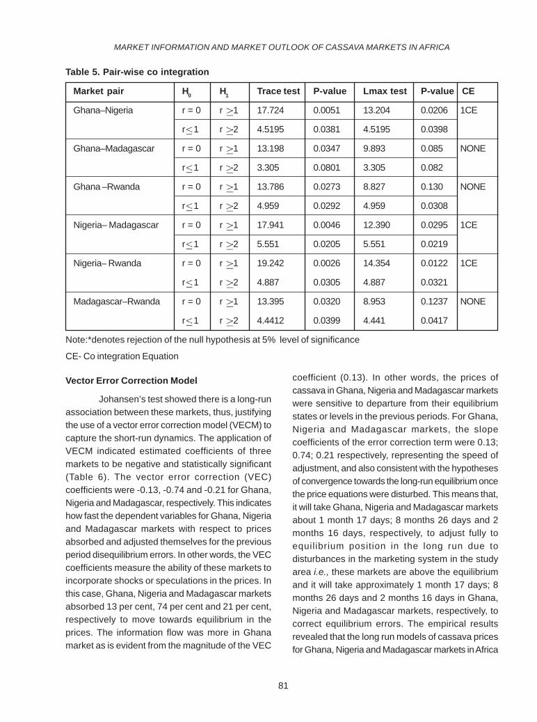
81
Table 5. Pair-wise co integration
Market pair H0 H1 Trace test P-value Lmax test P-value CE
Ghana–Nigeria r = 0 r 1 17.724 0.0051 13.204 0.0206 1CE
r 1 r 2 4.5195 0.0381 4.5195 0.0398
Ghana–Madagascar r = 0 r 1 13.198 0.0347 9.893 0.085 NONE
r 1 r 2 3.305 0.0801 3.305 0.082
Ghana –Rwanda r = 0 r 1 13.786 0.0273 8.827 0.130 NONE
r 1 r 2 4.959 0.0292 4.959 0.0308
Nigeria– Madagascar r = 0 r 1 17.941 0.0046 12.390 0.0295 1CE
r 1 r 2 5.551 0.0205 5.551 0.0219
Nigeria– Rwanda r = 0 r 1 19.242 0.0026 14.354 0.0122 1CE
r 1 r 2 4.887 0.0305 4.887 0.0321
Madagascar–Rwanda r = 0 r 1 13.395 0.0320 8.953 0.1237 NONE
r 1 r 2 4.4412 0.0399 4.441 0.0417
Note:*denotes rejection of the null hypothesis at 5% level of significance
CE- Co integration Equation
Vector Error Correction Model
Johansen’s test showed there is a long-runassociation between these markets, thus, justifyingthe use of a vector error correction model (VECM) tocapture the short-run dynamics. The application ofVECM indicated estimated coefficients of threemarkets to be negative and statistically significant(Table 6). The vector error correction (VEC)coefficients were -0.13, -0.74 and -0.21 for Ghana,Nigeria and Madagascar, respectively. This indicateshow fast the dependent variables for Ghana, Nigeriaand Madagascar markets with respect to pricesabsorbed and adjusted themselves for the previousperiod disequilibrium errors. In other words, the VECcoefficients measure the ability of these markets toincorporate shocks or speculations in the prices. Inthis case, Ghana, Nigeria and Madagascar marketsabsorbed 13 per cent, 74 per cent and 21 per cent,respectively to move towards equilibrium in theprices. The information flow was more in Ghanamarket as is evident from the magnitude of the VEC
coefficient (0.13). In other words, the prices ofcassava in Ghana, Nigeria and Madagascar marketswere sensitive to departure from their equilibriumstates or levels in the previous periods. For Ghana,Nigeria and Madagascar markets, the slopecoefficients of the error correction term were 0.13;0.74; 0.21 respectively, representing the speed ofadjustment, and also consistent with the hypothesesof convergence towards the long-run equilibrium oncethe price equations were disturbed. This means that,it will take Ghana, Nigeria and Madagascar marketsabout 1 month 17 days; 8 months 26 days and 2months 16 days, respectively, to adjust fully toequilibrium position in the long run due todisturbances in the marketing system in the studyarea i.e., these markets are above the equilibriumand it will take approximately 1 month 17 days; 8months 26 days and 2 months 16 days in Ghana,Nigeria and Madagascar markets, respectively, tocorrect equilibrium errors. The empirical resultsrevealed that the long run models of cassava pricesfor Ghana, Nigeria and Madagascar markets in Africa
MARKET INFORMATION AND MARKET OUTLOOK OF CASSAVA MARKETS IN AFRICA
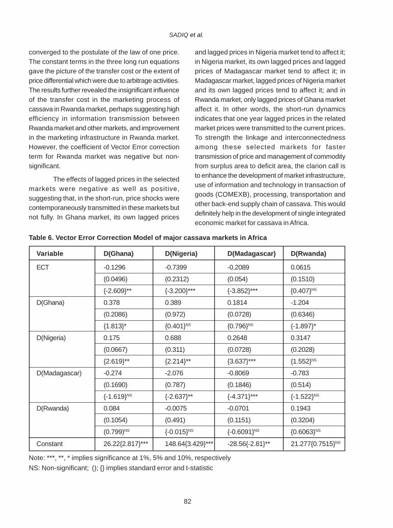
82
converged to the postulate of the law of one price.The constant terms in the three long run equationsgave the picture of the transfer cost or the extent ofprice differential which were due to arbitrage activities.The results further revealed the insignificant influenceof the transfer cost in the marketing process ofcassava in Rwanda market, perhaps suggesting highefficiency in information transmission betweenRwanda market and other markets, and improvementin the marketing infrastructure in Rwanda market.However, the coefficient of Vector Error correctionterm for Rwanda market was negative but non-significant.
The effects of lagged prices in the selectedmarkets were negative as well as positive,suggesting that, in the short-run, price shocks werecontemporaneously transmitted in these markets butnot fully. In Ghana market, its own lagged prices
and lagged prices in Nigeria market tend to affect it;in Nigeria market, its own lagged prices and laggedprices of Madagascar market tend to affect it; inMadagascar market, lagged prices of Nigeria marketand its own lagged prices tend to affect it; and inRwanda market, only lagged prices of Ghana marketaffect it. In other words, the short-run dynamicsindicates that one year lagged prices in the relatedmarket prices were transmitted to the current prices.To strength the linkage and interconnectednessamong these selected markets for fastertransmission of price and management of commodityfrom surplus area to deficit area, the clarion call isto enhance the development of market infrastructure,use of information and technology in transaction ofgoods (COMEXB), processing, transportation andother back-end supply chain of cassava. This woulddefinitely help in the development of single integratedeconomic market for cassava in Africa.
Table 6. Vector Error Correction Model of major cassava markets in Africa
Variable D(Ghana) D(Nigeria) D(Madagascar) D(Rwanda)
ECT -0.1296 -0.7399 -0.2089 0.0615
(0.0496) (0.2312) (0.054) (0.1510)
{-2.609}** {-3.200}*** {-3.852}*** {0.407}NS
D(Ghana) 0.378 0.389 0.1814 -1.204
(0.2086) (0.972) (0.0728) (0.6346)
{1.813}* {0.401}NS {0.796}NS {-1.897}*
D(Nigeria) 0.175 0.688 0.2648 0.3147
(0.0667) (0.311) (0.0728) (0.2028)
{2.619}** {2.214}** {3.637}*** {1.552}NS
D(Madagascar) -0.274 -2.076 -0.8069 -0.783
(0.1690) (0.787) (0.1846) (0.514)
{-1.619}NS {-2.637}** {-4.371}*** {-1.522}NS
D(Rwanda) 0.084 -0.0075 -0.0701 0.1943
(0.1054) (0.491) (0.1151) (0.3204)
(0.799)NS {-0.015}NS {-0.6091}NS {0.6063}NS
Constant 26.22{2.817}*** 148.64{3.429}*** -28.56{-2.81}** 21.277{0.7515}NS
Note: ***, **, * implies significance at 1%, 5% and 10%, respectivelyNS: Non-significant; (); {} implies standard error and t-statistic
SADIQ et al.

83
Granger Causality Test
After determining cointegration amongdifferent cassava markets, Granger causality wasalso estimated between the selected pairs of cassavamarkets in Africa. The Granger causality shows thedirection of price formation between two markets andrelated spatial arbitrage, i.e., physical movement ofthe commodity to adjust the prices difference. Theresults of Granger causality tests showed that allthe three F-statistics for the causality tests ofproducer prices in Nigeria market on other marketswere not statistically significant, thus, the nullhypothesis of no Granger causality was accepted ineach case for Nigeria market. Besides, Madagascarmarket had two, while Ghana and Rwanda marketseach had one F-statistics statistically significant onother market prices (Table 7).
According to the Granger causality tests,there were unidirectional causalities between these
market pairs: Rwanda-Nigeria, Ghana-Rwanda;Madagascar-Nigeria and Madagascar-Rwandamarkets, meaning that a price change in the formermarket in each pair Granger causes the priceformation in the latter market, whereas the pricechange in the latter market was not fed back by theprice change in the former market in each pair. Bi-directional causality was not observed, thus,indicating there was no perfect price transmissionmechanism between any cassava market pair.Further, two market pairs, Ghana-Nigeria andMadagascar-Ghana have no direct causality betweenthem, indicating that neither the former in each marketpair Granger causes the price formation in latter, northe latter in each market pair granger causes theprice formation in the former. In other words, therewas no long-run price transmission between thesemarket pairs.
Table 7. Pair wise Granger causality tests of selected markets
H0 T-stat Prob. Granger cause Direction
Ghana Nigeria 0.754 0.490 No None
Ghana Nigeria 0.098 0.907 No
Madagascar Ghana 0.284 0.757 No None
Madagascar Ghana 0.486 0.626 No
Nigeria Rwanda 0.961 0.408 No Unidirectional
Nigeria Rwanda 7.769 0.006** Yes
Rwanda Ghana 1.999 0.175 No Unidirectional
Rwanda Ghana 6.103 0.014** Yes
Madagascar Nigeria 4.296 0.037** Yes Unidirectional
Madagascar Nigeria 2.460 0.124 No
Rwanda Madagascar 1.196 0.333 No Unidirectional
Rwanda Madagascar 11.145 0.005** Yes
Note: **denotes rejection of the null hypothesis at 5% level of significance
MARKET INFORMATION AND MARKET OUTLOOK OF CASSAVA MARKETS IN AFRICA

84
VECM Diagnostic checking
Autocorrelation tests for all the selected marketsindicate that the residuals are free from serialcorrelation as evident from Ljung-Box Q-statisticswhich are not different from zero at 5 per centprobability level, meaning that the residuals are purelyrandom. Also, the Arch effects indicate that the errorterm have no arch effects as evident from the LM
test statistics which are not different from zero at 5per cent probability level. The tests of normalityindicate that the residuals are normally distributedas is clear from Doornik-Hansen test which is notdifferent from zero at 5 per cent probability level.Therefore, it can be inferred that the model usedcertified all the necessary criteria for it to be termedbest fit (Table 8).
Table 8. VECM Diagnostic checking
Test Statistic P-value
Autocorrelation Ljung-Box Q (Eq1) 4.872 0.0875
Ljung-Box Q (Eq2) 0.761 0.684
Ljung-Box Q (Eq3) 0.274 0.872
Ljung-Box Q (Eq4) 0.168 0.92
Arch effect LM-Test (Eq1) 2.594 0.273
LM-Test (Eq2) 3.256 0.196
LM-Test (Eq3) 1.452 0.484
LM-Test (Eq4) 0.517 0.772
Normality Doornik-Hansen test 11.038 0.1996
Impulse Response Functions
The results of impulse response functionsshow how and to what extent a standard deviationshock in one of the cassava markets affects thecurrent as well as future prices in all the integratedmarkets over a period of ten years. When the effectof a shock dies out over time, the shock is said tobe transitory and when the effect of a shock doesnot die out over time, the shock is said to bepermanent. It can be observed that when a standarddeviation shock is given to any market, the effectson other markets will either be permanent or transitoryi.e. the responses of other markets appear ordisappear between second and tenth years.
The graphs indicate that an orthogonalizedshock to the prices in Ghana market will havepermanent effect on the prices in Rwanda marketand transitory effects on the prices in Nigeria and
Madagascar markets; while an orthogonalized shockto the prices of cassava in Nigeria market will exerttransitory effects on Ghana and Madagascarmarkets, and a permanent on the price in Rwandamarket. According to this model, unexpected shocksthat are local to Madagascar market will havepermanent effects on the prices in Ghana and Nigeriamarkets, and a transitory effect on Rwanda market;while unexpected shock that are local to Rwandamarket would have only permanent effects on theprices in Ghana, Nigeria and Madagascar markets.A shock originating from the Ghana market wouldbe less transmitted to Nigeria and Madagascarmarkets, and more transmitted to Rwanda market,but a shock originating from Nigeria and Madagascarmarket would be relatively less transmitted to Ghanamarket, and relatively more transmitted to Ghanamarket if the shock originates from Rwanda market.Like Ghana market, a shock given to the Nigeria
SADIQ et al.

85
market would be transmitted to a lesser extent toother markets except Rwanda market, implying thatGhana and Nigeria markets would be relativelymarket followers and will not play a significant rolein international cassava markets of Africa. Animportant point to be noted is that the producer pricesin the Madagascar market is positively related toprices in Ghana and Nigeria markets and inversely
related to the prices in the Rwanda market. On theother hand, the results of Rwanda market impulseresponse confirm that the price transmission fromRwanda to other markets occur in large proportions,thus, implying that the Rwanda market hasdominance in price determination in other cassavamarkets (Fig. 1).
Fig. 1. Impulse response functions
MARKET INFORMATION AND MARKET OUTLOOK OF CASSAVA MARKETS IN AFRICA
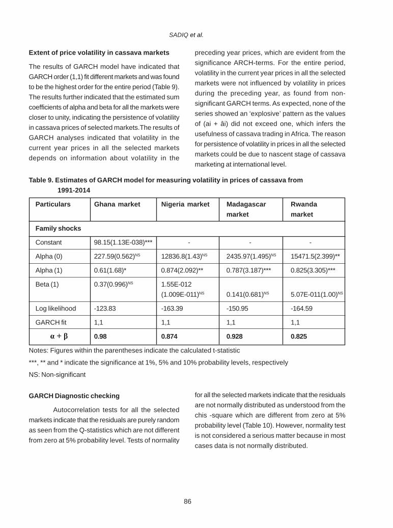
86
Extent of price volatility in cassava markets
The results of GARCH model have indicated thatGARCH order (1,1) fit different markets and was foundto be the highest order for the entire period (Table 9).The results further indicated that the estimated sumcoefficients of alpha and beta for all the markets werecloser to unity, indicating the persistence of volatilityin cassava prices of selected markets.The results ofGARCH analyses indicated that volatility in thecurrent year prices in all the selected marketsdepends on information about volatility in the
preceding year prices, which are evident from thesignificance ARCH-terms. For the entire period,volatility in the current year prices in all the selectedmarkets were not influenced by volatility in pricesduring the preceding year, as found from non-significant GARCH terms. As expected, none of theseries showed an ‘explosive’ pattern as the valuesof (ai + âi) did not exceed one, which infers theusefulness of cassava trading in Africa. The reasonfor persistence of volatility in prices in all the selectedmarkets could be due to nascent stage of cassavamarketing at international level.
Table 9. Estimates of GARCH model for measuring volatility in prices of cassava from 1991-2014
Particulars Ghana market Nigeria market Madagascar Rwandamarket market
Family shocks
Constant 98.15(1.13E-038)*** - - -
Alpha (0) 227.59(0.562)NS 12836.8(1.43)NS 2435.97(1.495)NS 15471.5(2.399)**
Alpha (1) 0.61(1.68)* 0.874(2.092)** 0.787(3.187)*** 0.825(3.305)***
Beta (1) 0.37(0.996)NS 1.55E-012(1.009E-011)NS 0.141(0.681)NS 5.07E-011(1.00)NS
Log likelihood -123.83 -163.39 -150.95 -164.59
GARCH fit 1,1 1,1 1,1 1,1
0.98 0.874 0.928 0.825
Notes: Figures within the parentheses indicate the calculated t-statistic
***, ** and * indicate the significance at 1%, 5% and 10% probability levels, respectively
NS: Non-significant
GARCH Diagnostic checking
Autocorrelation tests for all the selectedmarkets indicate that the residuals are purely randomas seen from the Q-statistics which are not differentfrom zero at 5% probability level. Tests of normality
for all the selected markets indicate that the residualsare not normally distributed as understood from thechis -square which are different from zero at 5%probability level (Table 10). However, normality testis not considered a serious matter because in mostcases data is not normally distributed.
SADIQ et al.

87
Table 10. Diagnostic checking for GARCH
Model Market ARCH-LM Test Normality Test (Chi2)
GARCH Ghana 0.7433 (0.989) 2.81 (0.000)
Nigeria 0.5809 (0.559) 43.7 (0.000)
Madagascar 0.5312 (0.943) 3.06 (0.002)
Rwanda 0.3836 (0.180) 2.73 (0.000)
Note: Values in parentheses are probability
Forecasting using ARIMA
Various combinations of the ARIMA models were triedafter first differencing of all the four series and basedon the smallest AIC value; the best ARIMA modelwas selected. Among all the ARIMA models tested,
ARIMA (0,1,1) model have the minimum AIC valuesfor price series of Ghana; Nigeria and Rwandamarkets, while ARIMA (1,1, 0) model has minimumAIC value for Madagascar market price series (Table11a).
Table 11a. AIC values of different ARIMA models
Market Criteria 1,1,1 1,1,0 0,1,1
Ghana AIC 213.8948 217.6009 211.9551**
BSC 218.4367 221.0074 215.3616
Nigeria AIC 286.3866 284.3922 284.3897**
BSC 290.9286 287.7987 287.7962
Madagascar AIC 229.0783 227.0941** 227.8623
BSC 233.6203 230.5006 231.2688
Rwanda AIC 261.8691 261.0318 260.9208**
BSC 265.2755 260.3028 263.1918
Note: **denotes best ARIMA model
Out of total 23 data points (1991 to 2014), first 18data points (from 1991 to 2009) were used for modelbuilding and the remaining 5 data points (from 2010to 2014) were used for model validation. One-stepahead forecasts of producer prices for all the selected
markets along with their corresponding standarderrors using naïve approach for the period 2009 to2014 (total 5 data points) in respect of above fittedmodels were computed (Table 11b).
MARKET INFORMATION AND MARKET OUTLOOK OF CASSAVA MARKETS IN AFRICA

88
Table 11b. One step ahead forecast of prices
Date Ghana market Nigeria market Madagascar Rwanda market market
Actual Forecast Actual Forecast Actual Forecast Actual Forecast
2010 168.95 156.58 142.45 113.93 172.44 184.65 312.27 314.33
2011 176.96 170.58 142.91 141.63 168.08 178.11 265.85 312.53
2012 184.00 183.89 152.55 141.24 170.00 174.94 297.21 271.84
2013 196.00 191.22 161.68 151.19 179.00 174.31 368.81 293.95
2014 210.00 201.70 171.00 160.30 200.00 180.44 337.23 359.20
The forecasting ability of ARIMA (0,1,1)models of price series for Ghana, Nigeria and Rwandamarkets; and forecasting capability of ARIMA (1,0,1)model for Madagascar market price series werejudged on the basis of mean absolute prediction error
(MAPE), relative mean absolute prediction error(RMAPE) and root mean square error (RMSE) values(Table 11c). A perusal of Table 11c reveals that for allthe price series for all the selected markets, RMAPEvalues were less than 10 per cent, indicating theaccuracy of the models used in the study.
Table 11c. Validation of models
Market MAPE RMSPE RMAPE (%)
Ghana 6.388 0.31608 3.48
Nigeria 12.46 1.582 8.22
Madagascar 0.586 0.729 0.711
Rwanda 5.904 5.4004 0.820
One step ahead out of sample forecast ofproducer prices of cassava for the above four marketsduring the periods 2015 to 2024 were computed. Theforecast values along with their corresponding lowerand upper 95 per cent confidence intervals are givenin Table 11d and Fig.2. As indicated, cassava pricesin Nigeria and Rwanda markets will be volatile duringthe periods from 2014 to 2024, as reflected by thewider confidence intervals associated with the ARIMAforecasts during this period. These imply that theconfidence intervals associated with the one-step-ahead out of sample forecasts during this period are
relatively large. Alternatively, while the confidenceintervals of cassava price forecasts for Ghana andMadagascar markets do fluctuate, they tend to bemore stable relative to the forecasts intervals forNigeria and Rwanda markets. These imply theconfidence intervals associated with the one-stepahead out of sample forecasts during these periodsare relatively smaller. This, in part, might reflect therelatively constant growth of the cassava productionduring the period 2015 to 2024. The fitted modelsalong with the predicted data points are also depictedin figures 2-5 to visualize the performance of fittedmodels.
SADIQ et al.

89
Table 11d. Out of sample forecast of cassava prices in selected markets
Year Ghana market Nigeria market
Forecast Upper CL Lower CL Forecast Upper CL Lower CL
2015 215.08 262.16 168.00 169.62 371.15 102.82
2016 222.91 280.18 165.64 167.91 457.39 147.69
2017 229.89 298.11 161.68 166.20 522.54 121.81
2018 237.13 314.12 160.15 164.49 576.99 110.47
2019 244.29 329.33 159.26 162.78 624.67 135.66
2020 251.48 343.81 159.15 161.07 667.55 158.41
2021 258.66 357.77 159.55 159.36 706.81 129.32
2022 265.84 371.29 160.39 157.65 743.21 128.76
2023 273.02 384.45 161.59 155.94 777.28 117.02
2024 280.20 397.30 163.10 154.23 809.40 134.28
Year Madagascar market Rwanda market
Forecast Upper CL Lower CL Forecast Upper CL Lower CL
2015 196.57 254.34 138.80 340.05 466.38 213.72
2016 203.05 270.25 135.85 340.05 507.63 172.47
2017 205.51 285.75 125.28 340.05 540.56 139.54
2018 209.60 299.25 119.96 340.05 568.81 111.29
2019 213.03 311.84 114.23 340.05 593.93 129.53
2020 216.73 323.67 109.79 340.05 616.78 141.19
2021 220.32 334.91 105.73 340.05 637.88 151.96
2022 223.96 345.68 102.23 340.05 657.58 162.01
2023 227.57 356.05 99.09 340.05 676.13 171.47
2024 231.19 366.08 96.31 340.05 693.71 180.44
Note: CL- Confidence Level
ARIMA Diagnostic Checking
The model verification is concerned with checkingthe residuals of the model to see if they containedany systematic pattern which still could be removedto improve the chosen ARIMA. The results ofautocorrelation tests for all the selected marketsindicate that the residuals are purely random asevidence from the Ljung-Box Q-statistics which arenot significantly different from zero at 5 percent
probability level (Table 12). This proved that theselected ARIMA (0,1,1) model for price series ofGhana, Nigeria and Rwanda markets; and ARIMA(1,1,0) model for Madagascar market wereappropriate model for forecasting. Also, the ARCHeffect tests showed no arch effects in the residualsas evident from Lagrange multiplier test which is notdifferent from zero at 5 percent probability level. Thenormality tests for all the selected markets indicate
MARKET INFORMATION AND MARKET OUTLOOK OF CASSAVA MARKETS IN AFRICA

90
that the residuals are not normally distributed asobserved from the Chi- square values which aresignificantly different from zero at 5% probability level(Table 12). However, normality test is not considered
as a serious matter because in most cases data arenot normally distributed. Therefore, the selectedmodels were the best fit.
Table 12. Diagnostic checking for best ARIMA models
Market ARIMA Autocorrelation test Normalitymodel (Ljung-Box Q) Arch test (LM) Test (Chi2)
Ghana 0,1,1 2.577(0.108) 2.939 (0.230) 0.414 (0.000)
Nigeria 0,1,1 0.0993 (0.753) 0.451(0.798) 13.16 (0.0014)
Madagascar 1,1,0 0.0358 (0.850) 4.715 (0.095) 2.895 (0.000)
Rwanda 0,1,1 2.982 (0.084) 2.702 (0.259) 6.511(0.038)
CONCLUSIONS
The study investigated cointegration,causality, price transmission, price volatility and priceforecasts among major cassava markets in Africa.ADF tests results indicated that all the price serieswere integrated of order 1. The results indicated thatdifferent cassava markets in Africa were well-integrated and have long-run price association acrossthem. The market pair-wise cointegration testconfirmed that all the market pairs did not have anyprice association between them, indicating that themajor cassava markets in Africa were poorlyintegrated when considered pair-wise. Someinferences were drawn from the market integration:Price transmission occurred due to the flow of marketinformation which was consequence of developmentin information technologies; the speed of convergencedepends on the market regulations and policychanges; and market integration is an indicator ofefficient functioning of markets. VECM resultsindicate that Ghana, Nigeria and Madagascar marketswere above the equilibrium, and it will takeapproximately 1 month 17 days; 8 months 26 daysand 2 months 16 days, respectively to correct theirrespective equilibrium error. Also, Granger causalitytests showed only four market pairs hadunidirectional causalities, while all the remaining
market pairs had no causal direction on priceformation between them. Situation of market pairbidirectional causality was not observed between themajor cassava markets in Africa. Further, results ofimpulse response functions confirmed that thespeeds as well as magnitude of shocks given toGhana and Nigeria markets were relatively lesstransmitted to other markets, thus indicating thesemarkets to be trend followers rather than trendsetters. This implies that the geographical situationand optimal distance between the market places holdthe mutual forces on commodity movements andprice formation. Therefore, the researchers advocatethat the network of agricultural producer marketsshould be well-designed so as to keep equal distancefrom each other, because it will not only boost adirect inter-market competition, but will also controlthe massive/high marketing margins of agriculturalcommodities. The produce can be moved to thedeficit areas thereby providing benefits to bothproducers and consumers. The extent of volatility incurrent prices due to family or internal shocks, asmeasured by the coefficients of GARCH model,indicated persistence volatility in all the markets, butnot of the explosive type, thus indicating usefulnessof cassava trading in Africa. Lastly, findings revealedthat the ARIMA model could be used successfully
SADIQ et al.
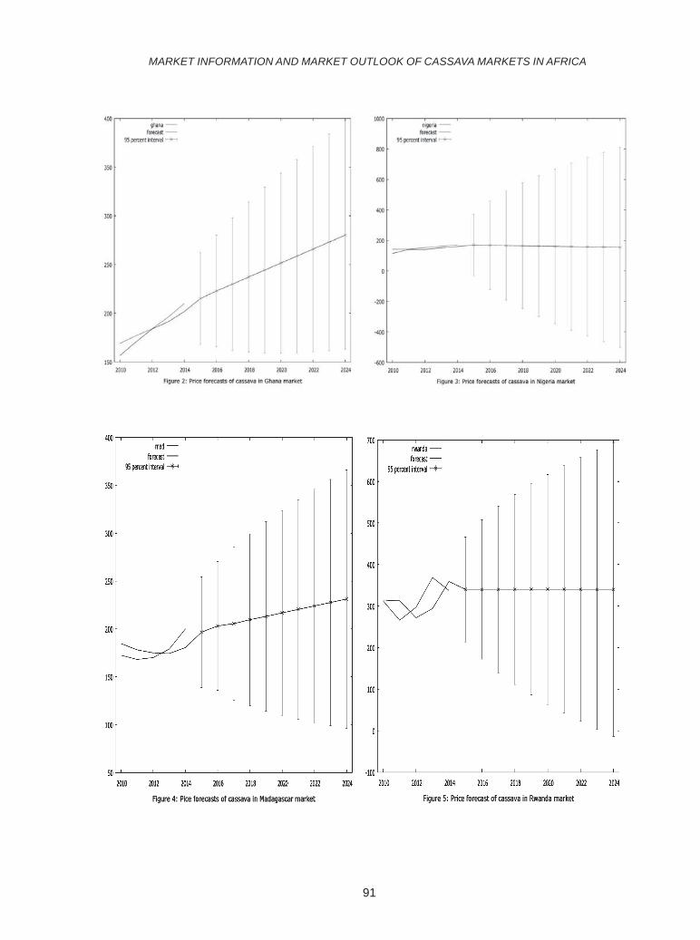
91
MARKET INFORMATION AND MARKET OUTLOOK OF CASSAVA MARKETS IN AFRICA
92
for modeling as well as forecasting of yearly producerprice of cassava in major cassava markets in Africa,given that the model has demonstrated a goodperformance in terms of explained variability andpredicting power. The findings of the present studywill serve as direct support for the potential use ofaccurate forecasts in decision-making for farmers,middlemen as well as consumers.
REFERENCES
Beag, F.A and Singla, N.2014.Cointegration, causalityand impulse response analysis in majorapple markets of India. AgriculturalEconomics Research Review. Vol.27(2):289-298.
Blay, J.K., Maiadua, S.U and Sadiq,M.S.2015.Horizontal market integration andprice transmission between m a i z e ,sorghum and millet in Dawanau market,Kano State, Nigeria: Evidence from non-linear vector error correction model. GlobalJournal of Agricultural Economics,Extension and Rural Development. Vol.3(10):330-337.
Granger, C.W.J.1969.Investigating causal relationsby econometric models and cross-spectralmethods. Econometrica: Journal of theEconometric Society. Vol. 37(1):424-438.
Ibana, S. E., Nkang, N.M and Ezedinma, C.2009.Price transmission and marketintegration: A test of the central markethypothesis of geographical markets forcassava products in Nigeria. Global Journalof Pure and Applied Sciences. Vol. 15(1):3-4.
Johansen, S. 1998. Statistical analysis ofcointegration vectors. Journal of economicdynamics and control. 12(2-3):231-254.
Koop, G., Pesaran, H and Potter, S.M.1996.Impulseresponse analysis in non-linear multivariate
models. Journal of Econometrics. Vol.74(1):119-148.
Kwasi, B.R and Kobina, B.J.2014. Cassava marketsintegration analysis in the central region ofGhana. Indian Journal of Economics andDevelopment, Vol. 10(4):319-329.
Ojiako, I.A., Ezedinma, C., Okechukwu, R.U andAsumugha, G.N.2013.Spatial integrationand price transmission in selected cassavaproducts’ markets in Nigeria: A case of Gari.World Applied Sciences Journal. Vol.22(9):1373-1383.
Ospina-Patino, M.T and Ezedinma, C. 2015.Understanding the linkage of urban and ruralmarkets of cassava products in Nigeria.Africa Journal of Agricultural Research. Vol.10(40):3804-3813.
Paul, R.K.2014.Forecasting wholesale price ofpigeonpea using long memory Time-Seriesmodels. Agricultural Economics ResearchReview. Vol. 27(2): 167-176.
Pesaran, H.H and Shin, Y. 1998. Generalized impulseresponse analysis in linear multivariatemodels. Economics Letters. Vol. 58(1):17-29.
Rahman, M.M and Shahbaz, M.2013.Do imports andforeign capital inflows lead EconomicGrowth? cointegration and causalityanalysis in Pakistan. South Asia EconomicJournal. Vol. 14(1): 59-81.
Sadiq, M.S., Singh, I.P., Suleiman Aminu, Umar,S.M., Grema, I.J., Usman, B.I., Isah, M.Aand Lawal, A.T.2016. Price transmis-sion,volatility and discovery of gram in someselected markets in Rajasthan state, India.International Journal of Environment,Agriculture and Biotechnology. Vol. 1(1):74-89.
SADIQ et al.

93
INTRODUCTION
For cultivated crops, conservation insitumeans continued cultivation and management byfarmers of crop populations in the agro systemswhere the crop has evolved. There are global effortson conservation of traditional resources and wisdom.
The public and private sector investmenttowards this goal is growing in India as well. Indiahas made significant progress in setting up a regimefor the management of its plant genetic resource(Biber-Klemm et al., 2005). India was endowed withmore than two lakh rice varieties, with Kerala as oneof the centres of diversity of rice. The antiquity ofrice cultivation in the state dates back to 3000 BC(Manilal, 1990). It is reported that nearly 2000traditional varieties were predominantly cultivated inKerala. Demographic, social, policy and climaticforces have triggered fast disappearance of many ofthese landraces, leading to fast erosion of thediversity base. Presently, the extent of coverage ofHigh Yielding Varieties (HYVs) of rice in the state isnearly 93%, which is dominated by a few varieties.The worry of substitution of diverse set of geneticallyvariable crop land races by a few genetically uniform
CONSERVATION OF TRADITIONAL RICE VARIETIES FOR CROPDIVERSITY IN KERALA
P. INDIRA DEVI, SEBIN SARA SOLOMON and MRIDULA NARAYANANDepartment of Agricultural Economics, College of Horticulture,
Kerala Agricultural University, Thrissur, Kerala- 680656
Date of Receipt: 25.2.2017 Date of Acceptance: 06.4.2017
ABSTRACTDespite the declining area and production under rice in Kerala over the past decade, a positive growth trend in
productivity is witnessed due to High Yielding Varieties (HYVs). The main objective of this study is to compare the social,economic, management and sustainability aspects of traditional varieties and HYVs of rice in general and to study their performanceunder the unique ecosystem of Pokkali, in Kerala. The tremendous decline in area of traditional varieties (-17.21%), reflected inthe output (-17.79%), dropping their productivity from 1842 tonnes per ha to 1645 tonnes per ha. On comparision, highestproductivity was seen for HYVs under irrigation (3845 kg ha-1) and the lowest productivity for traditional varieties (TVs) underrainfed condition (1522 kg ha-1).The results confirm the hypothesis that HYVs have a significant positive influence on the cropyield. When 1.38 per cent higher yield is estimated due to the adoption of HYVs, the risk is also high, 7.08 for HYVs and 6.12 percent for TVs. Still, some personal and economic attributes encourage the continued adoption of TVs, in small and marginal farmholdings. This facilitates developing effective policy for in-situ conservation of indigenous land races ensuring local participation.Thestrategies may include market/legal instruments or efforts in creating awareness and incentivizing the conservation efforts.
E-mail:[email protected]
J.Res. ANGRAU 45(2) 93-99, 2017
modern varieties is widely expressed in literature(Brush, 1991). It has translated into the creation ofgene banks around the world, i.e., ex situconservation (Plucknett et al., 1987). However, thereis a disadvantage that the genetic resourcesconserved ex situ are frozen at the evolutionary clockwhen they are collected (Jackson, 1995). Thisnaturally underlines the importance of in situconservation efforts.
This paper analyses the present status andtrend in the cultivation of traditional varieties (TVs)and HYVs of rice in Kerala. The relative productionmerits of traditional vs. high yielding varieties andthe societal behaviour towards conservation are alsodiscussed based on data from an ecologicallysensitive organic farming rice tract. The informationmay facilitate developing a suitable policy for in situconservation of indigenous land races.
MATERIAL AND METHODS
This paper involves analysis of both primaryand secondary data based on rice farming. The dataon area, production and productivity of (HYVs) and(TVs) published by Directorate of Economics and

94
Statistics, Government of Kerala for the period from1995 to 2011 was compiled and statisticallyanalysed. The average annual growth rate andcoefficient of variation was estimated.
The primary data was gathered from theidentified respondents of the prominent rice growingareas of the state. The study area, Pokkali tract isspread over 5,500 hectares throughout the districtsof Ernakulam, Thrissur and Alappuzha of Kerala inSouthern India. Pokkali (pronounced Pokkaalli) is aunique saline tolerant rice variety that is cultivatedin an organic way in the water-logged coastal regionsof Kerala. One season of rice is followed by prawnfarming thus facilitating nutrient recycling. Noexternal chemical or organic inputs are applied. Thus,the organically-grown Pokkali is famed for its peculiartaste and high protein content and it has got theGeographical Indication (GI) registration for itsuniqueness.
The data for the study was gathered throughpersonal interview method using structured interviewschedule. For this purpose, 37 farmers were randomlychosen and post-stratified based on the variety (HighYielding Variety /Traditional Variety) cultivated. Thisincluded farmers who have been cultivating traditionalvariety (Pokkali) and those are cultivating HYV(Vytilla 6) for the past 5- 10 years.
To quantify the contribution of technology(variety) and resource use efficiency in the HYV andTVs, Cobb-Douglas production function was fitted,
Y= aX1b1. X2
b2. X3b3eµ
where,
Y= output of rice (kg ha-1)
X1= seed rate (kg ha-1)
X2= labour (man days ha-1)
X3= variety as dummy variable (TV-0, HYV- 1)
ì= Random disturbance term in conformity with the OLS assumptions
bi= Slope parameter of regression function
a= Scale parameter
The social factors that influenced the farmer’sdecision to choose the variety were analyzedemploying the probit model:
Pi = 1 where Pi is the probability that 1 + e –z
i the farmers use traditional varieties
Pi = 1- 1 where Pi is the probability 1 + e –z
i that the farmers use HYVs
Taking logarithm on both sides,
Ln (Pi) = Zi = a + â i + Xi +ei
1-Pi
Where Xi is the vector of independentvariables and âi is are the coefficients to be estimated.The independent variables were the age, educationof the farmer and the area under rice cultivation. Itwas hypothesized that age and education havepositive influence on the selection of traditionalvarieties while the area under rice farming is havingnegative influence.
RESULTS AND DISCUSSION
Rice production scenario in Kerala
Kerala state, where the staple food is rice,is producing only one-fifth of the domesticrequirement. At the same time, area under ricecultivation and the production has been exhibiting adeclining trend over the past several years (1995-2011). Table 1 detail the trend in the area, productionand productivity of rice during this period. The averagerate of decline in area during the period 1995-2011 isestimated at 4.84 per cent per annum. In 1995-96the rice area was 4.71 lakh ha which had declined to2.13 lakh ha in 2010-11. The production has comedown from 9.53 lakh tonnes to 5.98lakh tonnes duringthe same period. The rate of decline was to the tuneof 3.68 per cent per annum.
The productivity of rice exhibits a positivegrowth trend at 1.48 per cent per annum which limitsthe external dependence to some extent. Thisincrease in productivity is mainly attributed to the
INDIRA DEVI et al.

95
coverage of High Yielding Varieties. Many highyielding/improved varieties are released by KeralaAgricultural University for the different riceecosystems of Kerala. Most widely acceptedvarieties include Uma, Jyothi, Jaya, Anaswara andMattaTriveni. The production from HYVs was reportedas 3.87 lakh tonnes in 1995-96, which increased to
4.98 lakh tonnes in 2010-11 at a growth rate of 1.59per cent per annum. The increase in HYV coverageduring the same period was 1.2 per cent per annum(1.64 lakh ha to 1.98 lakh ha) and the productivityimprovement was to the tune of 0.39 per cent perannum i.e. from 2362tonnes per hectare to 2513tonnes per hectare.
Table 1.Trend in rice production in Kerala (1995-2011)
Variety Area Production Productivity
HYV 1.20** 1.59*** .39***
Traditional -17.21*** -17.79*** -.70***
Total -4.84*** -3.68*** 1.48***
*** Significant at 1% level ** Significant at 5% level
Source : Farm Guide (2012)
Thus, it is clear that the decline in area andproduction is mainly in the case of TVs. The veryhigh rate of decline in area under cultivation is mainlyobserved in the case of TVs (-17.21%), which iscorrespondingly reflected in the output as well(-17.79%). Obviously, the productivity has also beendeclining from 1842 tonnes per hectare to 1645tonnes per hectare. The traditional varieties of Kerala,which were location specific, thus, slowlydisappeared causing erosion to the diversity baseand rich traditional wealth. The varieties in this groupare Pokkali, Cheruvirippu, Chettivirippu,Orumundakkan, Thavalakkannan, Chitteniand manyothers.
There are three major rice growing seasonsin Kerala, Autumn[1st season (April/May to Sept /Oct )] , Winter[2nd season ( Sept/Oct to Dec/ Jan )]and Summer [3rd season ( Dec/ Jan to March/ April)]. The TVs were mainly grown in winter season.During 1995-96, 56 per cent of TV coverage was in
winter season. The comparatively high straw yield(1:1grain: straw ratio in TVs and 2:1 in HYVs) in TVswas the major reason for the choice. The harvestingtime in winter was favourable for drying and stalkingthe straw for year round purpose. Consequent to thedecline in the livestock population (from 33.99 lakhin 1996 to 17.40 lakh in 2007) the demand for strawalso declined. This naturally might have triggered thereplacement of traditional varieties with HYVs evenin winter season. By 2010-11, coverage of TVs inwinter season has come down to 13,101 ha.However, the rate of decline was lowest in winter (-14.9%) compared to autumn (-23.39%) and summer(- 23.8%).
It is to be noted that the entire decline inrice area is in TV coverage during winter and summerseasons, whereas the HYV coverage is showing anincrease over years, the rate of increase beinghighest during winter season. Thus, extend of spreadof the HYV’s is more prominent in this season.
CONSERVATION OF TRADITIONAL RICE VARIETIES

96
Table 2. Season wise growth rate of rice area in Kerala (1995-2011)
Autumn Summer Winter Overall
HYV -0.21 2.65* 1.32 1.20**
Traditional -23.39*** -14.9*** -23.8*** -17.21***
* 10% level of significance ** 5% level of significance *** 1 % level of significance
Source : Farm Guide (2012)
Irrigation is a critical input in HYV cultivation,as it is a pre-condition for fertilizer use, especiallyduring winter and summer. Of the total rice area,63.31 per cent is irrigated (2004-05). HYVs are mainlygrown under irrigated condition, occupying 88 percent of total irrigated rice cultivation. Sixty-five percent of total rice production of Kerala is also from
irrigated area and the bulk of it is from HYVs (90.4%).Comparing the productivity between HYVs andtraditional varieties grown under irrigated and rainfedconditions, highest productivity was seen for HYVsunder irrigation (3845 kg ha-1) and the lowestproductivity for traditional varieties grown under rainfedcondition (1522 kg ha-1), which is expected(Table 3).
Table 3. Season wise area, production and productivity of rice in Kerala (2004-05)
HYV TV
Irrigated Rainfed Irrigated Rainfed
Area (in ha)
Autumn 20798 58210 893 6897
Winter 105514 14059 20787 12476
Summer 35184 4717 425 1
Total 161496 76986 22105 19374
Production (in tonnes)
Autumn 522337 178353 1046 10088
Winter 250535 22911 39759 22324
Summer 88794 350 607 1
Total 391666 201614 41412 32413
Productivity (kg ha-1)
Autumn 3830 3537 1783 2226
Winter 3614 3447 2911 2724
Summer 3845 3319 2866 1522
Source : Farm Guide (2012)
VarietySeason
Variety
Season
INDIRA DEVI et al.
97
Difference in area, production andproductivity can be seen for the three seasons in thecase of HYVs and TVs under irrigated and non-irrigated conditions. For HYVs grown non irrigatedsituation, crop productivity is more in summerseason. Under rainfed conditions HYVs were grownextensively in autumn season compared to winterand summer. The production (178,353 tones) andproductivity (3537 kg ha-1) is also highest in thisseason. Hence, it can be concluded that for HYVs,highest productivity can be observed in summerseason if it is irrigated and under rainfed condition,productivity is higher in autumn season.
In the case of traditional varieties highestarea (20,787 ha), production (39,759 tonnes) andproductivity (2911 kg ha-1) was observed in winterseason, under irrigated condition. However, the areaunder TVs during winter season has been reducingat the rate of -14.9 per cent. The situation was thesame under rainfed conditions too i.e., the highestarea, production and productivity was observed inwinter season. The productivity of TVs was observedto be highest in winter season, both under irrigatedand rainfed conditions. At the same time, the extendof coverage of the varieties shows a decline in thisseason, over the years.
Thus, it can be concluded that the declinein rice area is mainly in the cultivation of TVs. Evenwhen the threat of water scarcity and climate changeimpacts are predicted, the spread of HYVs are fast.The decline of area under traditional varieties in winterseason is a major matter of concern, as it was themajor season during which traditional varieties weregrown and the performance was best.
The Varietal effect
The improved varieties released by KAU fromRice Research Station, Vytilla, which is the stationfor rice research in the Pokkali tracts of Kerala areVytilla 1, Vytilla 2, Vytilla3, Vytilla 4, Vytilla 5, Vytilla6, Vytilla 7 and Vytilla 8 of which Vytilla 6 is the
most popular among the respondent farmers. Thetraditional variety Pokkali was grown by 23 farmers.
The management of Pokkali cultivationfollows organic methods, mainly due to geographicalpeculiarities. The land is prepared by strengtheningbunds and making mounds of 1m height and 0.5mbase on which seeds are sown. The seed raterecommended for Vytilla varieties are 100 kg ha-1andfor local variety is 80-100 kg ha-1. The seeds aresprouted on the mounts and when the seedlingsreach the height of 40-45 cm (in 30-35 days), themounds are cut into pieces with a few seedlings,which are uniformly spread in the field. Later the gapfilling is done.
Generally, chemical fertilizers are not usedin Pokkali cultivation. Organic manure content inthese soils is reported to be high due to shrimpfarming and crop residue of the previous crop. Hence,they do not apply any organic manure. Weeding isthe only intercultural operation performed. Harvestingis done by cutting only the panicles leaving the restof the biomass for decaying. Thus, there is nodifference in management practices between thesetwo groups. The socio-economic status of the ricefarmers showed that more than 50 per cent of thefarmers are above 50 years of age. More than three-fourth of the respondents had schooling less thantwelve years. The average family size is 4- 5 membersper family.
The production response of Vytilla andPokkali varieties was examined with the help ofCobb-Douglas Production function fitted to the crosssectional farm level data collected from the farmers.The production function was estimated using OrdinaryLeast Square Technique. The estimates are given inthe Table 4. The result of the analysis pooling theobservation confirms the hypothesis that HYVs hasa significant positive influence on the crop yield. Thecoefficient estimates the increase in yield at 1.38per cent higher due to the adoption of HYVs comparedto traditional varieties. This naturally acts as a strong
CONSERVATION OF TRADITIONAL RICE VARIETIES
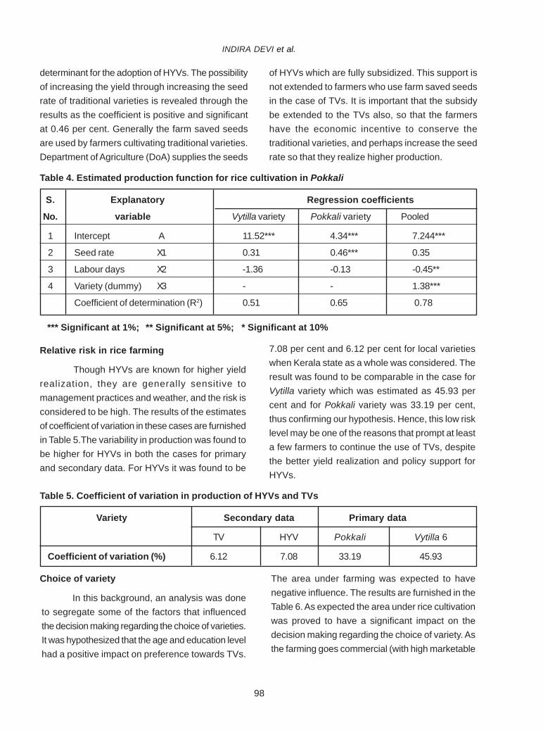
98
Choice of variety
In this background, an analysis was doneto segregate some of the factors that influencedthe decision making regarding the choice of varieties.It was hypothesized that the age and education levelhad a positive impact on preference towards TVs.
The area under farming was expected to havenegative influence. The results are furnished in theTable 6. As expected the area under rice cultivationwas proved to have a significant impact on thedecision making regarding the choice of variety. Asthe farming goes commercial (with high marketable
determinant for the adoption of HYVs. The possibilityof increasing the yield through increasing the seedrate of traditional varieties is revealed through theresults as the coefficient is positive and significantat 0.46 per cent. Generally the farm saved seedsare used by farmers cultivating traditional varieties.Department of Agriculture (DoA) supplies the seeds
of HYVs which are fully subsidized. This support isnot extended to farmers who use farm saved seedsin the case of TVs. It is important that the subsidybe extended to the TVs also, so that the farmershave the economic incentive to conserve thetraditional varieties, and perhaps increase the seedrate so that they realize higher production.
Table 4. Estimated production function for rice cultivation in Pokkali
S. Explanatory Regression coefficients
No. variable Vytilla variety Pokkali variety Pooled
1 Intercept A 11.52*** 4.34*** 7.244***
2 Seed rate X1 0.31 0.46*** 0.35
3 Labour days X2 -1.36 -0.13 -0.45**
4 Variety (dummy) X3 - - 1.38***
Coefficient of determination (R2) 0.51 0.65 0.78
*** Significant at 1%; ** Significant at 5%; * Significant at 10%
Relative risk in rice farming
Though HYVs are known for higher yieldrealization, they are generally sensitive tomanagement practices and weather, and the risk isconsidered to be high. The results of the estimatesof coefficient of variation in these cases are furnishedin Table 5.The variability in production was found tobe higher for HYVs in both the cases for primaryand secondary data. For HYVs it was found to be
7.08 per cent and 6.12 per cent for local varietieswhen Kerala state as a whole was considered. Theresult was found to be comparable in the case forVytilla variety which was estimated as 45.93 percent and for Pokkali variety was 33.19 per cent,thus confirming our hypothesis. Hence, this low risklevel may be one of the reasons that prompt at leasta few farmers to continue the use of TVs, despitethe better yield realization and policy support forHYVs.
Table 5. Coefficient of variation in production of HYVs and TVs
Variety Secondary data Primary data
TV HYV Pokkali Vytilla 6
Coefficient of variation (%) 6.12 7.08 33.19 45.93
INDIRA DEVI et al.

99
Table 6. Estimated logit regression coefficients of factors influencing the choice of traditional variety
CONCLUSION
The rice cultivation in Kerala is facing seriouschallenges. The shrinking area under rice farming isattributed to demographic, social, economical andpolitical factors. The general decline in area undercultivation, wiped out the traditional varieties at afaster pace due to obvious reasons of policy supportand relative economics in favour of HYVs. Thesituation is no different in Pokkali area as well. Thebetter yield realization and policy factors favour thespread of Vytilla varieties (HYVs) despite higher levelsof risk. The cultivation of local varieties is slowlygetting confined to small and marginal rice holdings,for subsistence income and domestic consumption.The policy intervention at this juncture warrantsfocused efforts for conservation of the traditionalvarieties. All the supports extended to HYVs are tobe extended to TVs (farm saved seeds) and thereshould be institutional arrangements to market theorganically grown and locally preferred varieties tobe procured at higher price to compensate for thedifference in yield. The incentive for conserving thetraditional variety can be considered as the policyinstrument.
REFERENCES
Biber-Klemm, S., Cottier, T., Cullet, P and Berglas,D.S. 2005.The current law of plant geneticresources and traditional knowledge. In:Right to Plant Genetic Resources andTraditional Knowledge. Biber-Klemm, S.,Cottier, T., Cullet, P. and Berglas, D.S.(Eds.). 4th Edition. Oxfordshire: CABinternational: pp. 56-111.
Brush, S.B. 1991. Farmer based approach toconserving crop germplasm. EconomicBotany. 45(2): 153-165.
Farm Guide. 2012. Directorate of Economics andStatistics, Government of Kerala. pp.11-21.
Jackson, M.T. 1995. Protecting the heritage of ricebiodiversity. Geojournal. 35: 267-274.
Manilal, K.S. 1990.Ethnobotany of rices of Malabar.In: Contribution to ethno botany. Jain, S.K.(Ed.). Scientific Publishers, Jodhpur. pp.243 – 253.
surplus) the tendency is to go for HYVs. At lowerlevel, subsistence farming, where area under farmingis small, the marketable surplus is low. Thus, thesmall and marginal farmers may prefer low risk
strategies to ensure the farm income, throughchoosing the TVs. Thus, the coverage of the Pokkalivariety is restricted to only small/marginal farms.Further, the TV Pokkali is preferred for its specialculinary properties, taste and qualities.
S.No. Variable (Xi) Coefficient ( ) Standard Error
1 Constant -1.180 1.643
2 Age (years) .145 0.389
3 Education .703 0.874
4 Rice area (in ha) -.579* 0.433
*Significant at 10%
CONSERVATION OF TRADITIONAL RICE VARIETIES

100
INTRODUCTION
A majority of the world’s poor belong toagricultural based rural households. Small andmarginal farmers in India constitute 85 per cent ofthe operated holdings and are cultivating 44.5 percent of operated area. While indebtedness is oftencited as the immediate reason for distress (ReserveBank of India, 2006; Satish, 2007) and deeper issueswere related to lower scale of operation, lack ofinformation, poor communication linkages with thewider markets and consequent exploitation byintermediaries in procuring inputs and marketing freshproduce, access to and cost of credit (Dev, 2005)and in isolated cases aggressive loan recoverypractices (Sriram, 2008).
A variety of approaches had emerged toresolve the problems faced by small and marginalfarmers like formation of co-operative credit societies,private participation promoted through contractfarming and encouraging different forms of communityorganizations like Self Help Groups (SHGs), CommonInterest Groups (CIGs), Farmers clubs, NewGeneration Co-operatives (NGC) and producercompany (PC) the newly emerged concept. It is new
MARKETING EFFICIENCY AND MARKET COMPETITIVENESS OF FARMERPRODUCER COMPANIES (FPCs) - A CASE OF
TELANGANA AND KARNATAKA STATES
M.KANDEEBAN and Y.PRABHAVATHIInstitute of Agribusiness Management, Acharya N.G. Ranga Agricultural University, Tirupati – 517 502
Date of Receipt: 17.4.2017 Date of Acceptance:30.5.2017
ABSTRACT India is predominantly dominated by small and marginal farmers and the growing trend of sub-division and fragmentation
of landholdings continues to fuel the proliferation of small and marginal farmers. The concept of Farmer Producer Companies(FPCs) is a way forward to address several problems of small and marginal farmers. Two farmer producer companies (FPCs)from Karnataka state and three FPCs from Telangana state were taken for the study. Marketing costs, marketing margins,marketing efficiency and price spread were analyzed from the major two marketing channels viz., FPC channel and Farmerschannel. It was observed that marketing efficiency and producer share in consumer rupee was higher in FPC channel due toreduction in transaction costs. Moreover, FPC farmers received better prices compared to MSP and modal prices in bothTelangana and Karnataka states for the year 2014-15 compared to 2015-16, which indicates farmers forming as producercompanies have added advantages in terms of increase in income level and supply chain efficiency .
J.Res. ANGRAU 45(2) 100-107, 2017
E-mail:[email protected]
legal entity of the producers of any kind, viz.,agricultural produce, forest produce, artisanproducts, and any other local produce where themembers are primary producers and company to beregistered as per companies Act of 1956. CurrentlyFarmer Producer Companies (FPCs) work indynamic, ever evolving market economies andpromote entrepreneurial spirit. A majority FPCs beingoperated in India were mainly driven to improve theefficiency of supply chain and thereby reducemarketing costs. Against this background the studywas undertaken with the following objectives. Thedata collected pertains to agricultural year 2015-16.The objectives of the study are to analyse themarketing costs and marketing margins incurred byFPCs, to analyze the marketing efficiency and pricespread of FPCs and to estimate the marketcompetitiveness of the FPCs.
Producer Organisations
Producer organizations are formal ruralorganizations whose members organized themselveswith the objective of improving farm income throughimproved production, marketing, and local processingactivities (Rondot and Collion, 2000). The main goal

101
of the producer organisation was to provide servicesthat support producers in their farming activities,including the marketing of the farm products. (Bijmanand Wollni, 2008). Producer company as a newanswer in not only rectifying the imperfect experiencesof cooperatives but also strengthening the leverageof small and marginal farmers through collectivemeans, and integrating their livelihoods intoremunerative markets. (Shylendra, 2009)
Market Competitiveness
The competitiveness rests on cost reductionstrategies which can be achieved through economiesof scale, either in terms of input provision, technicalassistance or commercial logistic through farmer’sorganization (Estelle and Danies, 2005). The FarmerProducer Organizations (FPO) were best structuresin eliminating the various transaction costs ofmarketing in the economy using the tools ofTransaction Cost Economics (TCE) (Varun Prasad,
2013). Farmer organisations have the potential toimprove services and reduce transaction costs, butissues such as downward accountability, poormanagement need to be addressed (Robert andPeter, 2014)
MATERIAL AND METHODS
From the total list of farmers’ producer companiesavailable in Small Farmers Agribusiness Consortiumwebsite (SFAC), the producer companies existingin Karnataka and Telangana states were taken andclassified based on various promoters involved in it.Out of total eight and nine FPCs in Karnataka andTelangana States, purposively three FPCs fromMahabubnagar district of Telangana and two fromBijapur district of Karnataka states were selectedsince these FPCs were promoted by the samepromoter. The FPCs under study were growing onesingle crop i.e. redgram. A set of pre-tested scheduleswere used to collect pertinent data from farmershareholders.
District Name of the FPCs
Bijapur(Karnataka) 1. Kalkeri Farmers services producer company( KFSPC)
2 . Jalwad Farmers services producer company ( JFSPC)
Mahabubnagar 1. Angadiraichur Farmers services producer company ( AFSPC)(Telangana) 2. Hasnabad Farmers services producer company ( HFSPC)
3. Kodangal Farmers services producer company ( KFSPC)
Marketing Cost
The actual expenses incurred (handling charges,assembling charges, transport and storage costs,expenses incurred for secondary services) in bringingthe produce from producers to consumers constitutemarketing costs.
The Marketing cost was estimated with the help offollowing formula
C = CF + Cm1 + Cm2 +Cm3 + ......... + Cmi ————-1
Where,
C = Total cost of marketing (Rs q-1)
CF = Cost paid by the producer (Rs q-1)
Cmi = Cost incurred by the ith middle in theprocess of marketing (Rs q-1)
Marketing Margin
Marketing margins are costs of equipment,transport, labour, capital, risk, and management. Itis the summation of share earned by various marketintermediaries for moving the produce from producerto consumer in a marketing channel.
KANDEEBAN and PRABHAVATHI

102
Marketing Efficiency
The Marketing efficiency of differentMarketing channels considered under the study wasestimated by Acharya and Agarwal’s Approach
ME = FP / (MC + MM) —————— 2
Where,
ME = Index of marketing efficiency
FP = Price received by the farmer
MC = Total marketing costs
MM = Net marketing margins
Producers Share in Consumers’ Rupee
It is the price received by the producerexpressed as percentage of the retail price (pricepaid by the consumer). If Pr is the retail price and Pfis the producers’ price, then the producers’ share inconsumers’ rupee (Ps) may be worked out as follows;
Ps = (Pf / Pr) * 100 ———————— 3
Where,
Ps = Producers’ share in consumers’ rupee
Pf = Price received by the producer
Pr = Price paid by the consumer
RESULTS AND DISCUSSION
i) Marketing Channels
The following marketing channels were beingoperated majorly in the study area in marketingof redgram.
(i). Farmers – Commission Agent – Trader – Miller– Wholesaler – Retailer – Consumer
(ii). Farmers – Farmer Producer Company - Trader- Miller – Wholesaler – Retailer – Consumer
ii) Analysis of Marketing costs and MarketingMargins
a) Marketing Costs
The costs involved in marketing of redgram inchannel I and Channel II were analyzed andresults are presented in table 1.
Table 1. Analysis of marketing costs under different channels in the marketing of red gram (Rs q-1)
Marketing Costs (Rs q-1)
S. No Functionaries Traditional Marketing FPC (Channel II)(Channel I)
1 Producer – Farmer 240 (8.78) 25 (1.1)
2 Commission Agent 102 (3.73) 0
3 Farmer Producer Company 0 38 (1.54)
4 Trader 190 (6.95) 190 (7.71)
5 Processor 1805 (66.06) 1805 (73.28)
6 Wholesaler 185 (6.77) 185 (7.51)
7 Retailer 210 (7.68) 210 (8.53)
8 Total 2,732 (100) 2,463 (100)
(Figures in parentheses indicate the percentages to total costs incurred)
MARKETING EFFICIENCY AND COMPETITIVENESS OF FARMER PRODUCER COMPANIES

103
It is observed from Table1 that totalmarketing cost incurred for redgram in Channel Iwas Rs. 2732/- per quintal and in channel II was Rs.2463/- per quintal. It implied that farmers whodisposed the produce on their own incurred relativelymore costs (Rs.269 q-1) compared to the FPCshareholder farmers. Within the channel, marketing
cost incurred by the processor was more comparedto other market functionaries followed by retailer,trader, wholesalers and commission agents.
b) Marketing margins
The marketing margins incurred in marketingof redgram in Channel I and Channel II wereanalyzed and results are presented in Table 2.
Table 2. Analysis of marketing margins under different channels in the marketing of redgram (Rs Q-1)
Marketing Margin (Rs q-1)
S. No Functionaries Traditional Marketing FPC(Channel I) (Channel II)
1 Producer – Farmer 0 0
2 Commission Agent 138 (14.55) 0
3 Farmer Producer Company 0 105(11.47)
4 Trader 110 (11.6) 110 (12.02)
5 Processor 395(41.66) 395(43.16)
6 Wholesaler 115 (12.13) 115(12.56)
7 Retailer 190 (20.04) 190(20.76)
8 Total 948(100) 915(100)
(Figures in parentheses indicate the percentages to total margins incurred)
It is inferred from Table 2 that the marginsearned in marketing of redgram through Channel II(Rs.915/-) was less than Channel I (Rs.948/-), whichimplied that the when the farmer was selling hisproduce to FPC, marketing margins earned by marketfunctionaries is minimized (3%). Compared to totalmarketing margins, margins earned by processors,traders, wholesalers and retailers were more inchannel II and channel I.
iii) Analysis of Marketing Efficiency and PriceSpread
a) Marketing Efficiency
Marketing efficiency is the measure ofavailability of information to all the participantsin a market that provides maximumopportunities to buyers and sellers to effecttransaction with minimum transaction costs.The results of marketing efficiency arepresented in Table 3.
KANDEEBAN and PRABHAVATHI
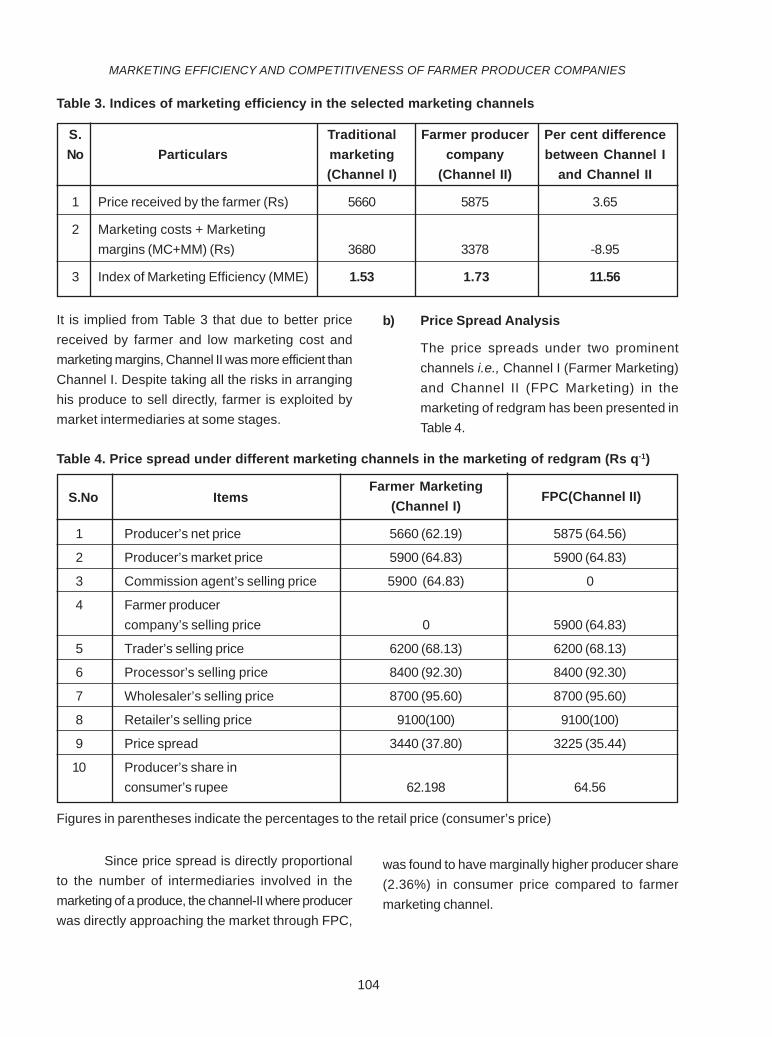
104
Table 3. Indices of marketing efficiency in the selected marketing channels
S. Traditional Farmer producer Per cent differenceNo Particulars marketing company between Channel I
(Channel I) (Channel II) and Channel II
1 Price received by the farmer (Rs) 5660 5875 3.65
2 Marketing costs + Marketingmargins (MC+MM) (Rs) 3680 3378 -8.95
3 Index of Marketing Efficiency (MME) 1.53 1.73 11.56
It is implied from Table 3 that due to better pricereceived by farmer and low marketing cost andmarketing margins, Channel II was more efficient thanChannel I. Despite taking all the risks in arranginghis produce to sell directly, farmer is exploited bymarket intermediaries at some stages.
b) Price Spread Analysis
The price spreads under two prominentchannels i.e., Channel I (Farmer Marketing)and Channel II (FPC Marketing) in themarketing of redgram has been presented inTable 4.
Table 4. Price spread under different marketing channels in the marketing of redgram (Rs q-1)
Farmer Marketing(Channel I)
1 Producer’s net price 5660 (62.19) 5875 (64.56)
2 Producer’s market price 5900 (64.83) 5900 (64.83)
3 Commission agent’s selling price 5900 (64.83) 0
4 Farmer producercompany’s selling price 0 5900 (64.83)
5 Trader’s selling price 6200 (68.13) 6200 (68.13)
6 Processor’s selling price 8400 (92.30) 8400 (92.30)
7 Wholesaler’s selling price 8700 (95.60) 8700 (95.60)
8 Retailer’s selling price 9100(100) 9100(100)
9 Price spread 3440 (37.80) 3225 (35.44)
10 Producer’s share inconsumer’s rupee 62.198 64.56
Figures in parentheses indicate the percentages to the retail price (consumer’s price)
Since price spread is directly proportionalto the number of intermediaries involved in themarketing of a produce, the channel-II where producerwas directly approaching the market through FPC,
was found to have marginally higher producer share(2.36%) in consumer price compared to farmermarketing channel.
FPC(Channel II)S.No Items
MARKETING EFFICIENCY AND COMPETITIVENESS OF FARMER PRODUCER COMPANIES

105
iii) Market Competitiveness
Marketing competitiveness of FPC over otherfarmers was analyzed taking intoconsideration Minimum support price (MSP),FPC selling price and open market price forredgram prevailing for the year 2013-14 and
2014-15 in Telangana and Karnataka statesand results are presented in the tables shownbelow. The modal prices prevailing in Tandurmarket of Telangana and Gulbarga market ofKarnataka for redgram were taken as they aremajor markets for redgram in respectivestates.
Table 5. Red gram prices in Telangana and Karnataka (2014-15)
Month/ Market MSP (Rs q-1) FPC selling price Modal price(Rs q-1) (Rs q-1)
Red gram prices in Telangana (2014-15)
December 4350 5472 4997.73
January 4350 5323 4847.98
February 4350 5172 5854.41
Average 4350 5323.33 5233.37
Red gram prices in Karnataka (2014-15)
December 4350 5470.1 4874.64
January 4350 5322.5 5151.70
February 4350 5172.2 5831.29
Average 4350 5321.6 5287.21
It is observed from the Table 5 that FPCsselling price for the year 2014-15 in the state ofTelangana and Karnataka were higher than that ofboth MSP (Rs.4350/Qn) and average modal price.Though the market committee ensures care to gradethe produce brought for sale by the farmers, yet thesystem has some limitations, which does not reflecttruly on the quality of the produce. Such limitationsare overcome in the FPCs in which the farmers wererewarded with better price for their produce. The year2014-15 incidentally happens to be a bright year for
pulses in general. The price received by the farmersis quite encouraging. But it was not the same storyin the year 2013-14, during which period the redgramprices were more often less than the MSP. This couldbe observed from the Table 6 that the price of redgramin open market was less compared to MSP. Thisproblem was fixed to certain extent by theinvolvement of FPCs through SFAC, which procuredthe members produce at MSP. This is also could beput forth on the positive side because the pricereceived in the open market was very discouraging.
KANDEEBAN and PRABHAVATHI

106
Red gram prices in Karnataka (2013-14)
December 4300 4300 3894.28
January 4300 4300 4030.38
February 4300 4300 4000.85
Average 4300 4300 3975.17
CONCLUSIONS
The disadvantages they face are high unittransaction costs in almost all non-labourtransactions. The study undertaken on FPCsrevealed that they not only help farmers buy or sellbetter due to scale benefits but also lowerstransaction cost for sellers and buyers besidesproviding technical help in production and creatingsocial capital. As encouraging the formation of FPChas many advantages, state governments, NGOsand other stake holders involved for the benefit offarming community should play an active role inmotivating farmers to organize themselves as FPCand render all sort of technical, financial, marketing, capacity building and mentoring assistance for theirsustenance in long run.
REFERENCES
Bijman, J and Wollni, M. 2008. Producerorganizations and vertical coordination: aneconomic organization theory perspective.Paper presented at the InternationalConference on Cooperative Studies (ICCS).Köln. October, 2008. pp. 1-17.
Dev, S. M. 2005. Agriculture and rural employmentin the budget. Economic and PoliticalWeekly. 40(14): 1410-1418.
Estelle, B and Denis, S. 2005. The role of small scaleproducer organisations to address marketaccess. Centre de CooperationInternationale en Recherché Agronomiquepour le Developpment, CIRD TERA. 1 (60/5): 73.
Table 6. Red gram prices in Telangana and Karnataka (2013-14)
Month/ Market MSP FPC selling price Modal price(Rs q-1) (Rs q-1) (Rs q-1)
Red gram prices in Telangana (2013-14)
December 4300 4300 3784.37
January 4300 4300 4167.30
February 4300 4300 3990.85
Average 4300 4300 3979.84
MARKETING EFFICIENCY AND COMPETITIVENESS OF FARMER PRODUCER COMPANIES
107
Reserve Bank of India. 2006. Report of the WorkingGroup to Suggest Measures to AssistDistressed Farmers.02 June 2014. Retrievedfrom website (http://rbidocs.rbi.org.in/rdocs/PublicationReport/Pdfs/78889.pdf) on10.4.2017.
Robert, M. M and Peter, D. 2014. Privatisation,empowerment and accountability: What arethe policy implications for establishingeffective farmer organisations. Land UsePolicy. 36: 285– 295.
Rondot, P and Collion, M.H. 2000. AgriculturalProducer Organizations: Their Contributionto Rural Capacity Building and PovertyReduction. Report of a Workshop,Washington, D.C., June 28-30. 1999:81.
Satish, P. 2007. Agricultural credit in the post-reformera: A target of systematic policy coarctation.Economic and Political Weekly: pp.2567-2575.
Shylendra, H. S. 2009. New Governance andDevelopment, Challenges of AddressingPoverty and Inequality. AcademicFoundation, New Delhi.
Sriram, M. 2008. Agrarian distress and rural credit:Peeling the onion. State of India’sLivelihoods: The 4P Report, AccessDevelopment Services. New Delhi: 177-188.
Varun Prasad. 2013. CCS working Paper 293 -Contract Farming through Farmer ProducerOrganizations (FPOs) in India. July, 2013.pp. 1-46.
KANDEEBAN and PRABHAVATHI

108
INTRODUCTION
Knowledge is key ingredient in applicationof any technology. It reflects an array of informationpossessed by an individual. It plays a pivotal role inunderstanding the intricacies involved in any givenphenomena. The Krishi Vigyan Kendra (KVK)s arerendering a great help to the farmers in increasingthe level of knowledge on various crops, theseinstitutions conducting different programmes toenlighten the farmers on various crop productiontechnologies. Rice is one of the main crops ofKarimnagar district and the present paper focuseson knowledge mapping of the farmers on riceproduction technologies in Karimnagar district.
MATERIAL AND METHODS
Ex-post facto research design combined withexploratory type of research design was used, asthe selected phenomena have already occurred andthe researcher had no control over the same. TheKVK Jammikunta of Telangana State (FormerlyAndhra Pradesh) along with its 15 adopted villageswas selected for the study (2013-14). A sample of60 rice growing farmers who are adopting the KVKtechnologies and 30 rice farmers who are not coveredunder KVK production technologies were selectedfrom the adopted villages. A schedule was developed
KNOWLEDGE MAPPING ON RICE ( Oryza sativa L.) PRODUCTIONTECHNOLOGIES BY THE FARMERS OF KARIMNAGAR DISTRICT IN
TELANGANA STATEN. VENKATESHWAR RAO, P.K. JAIN, N. KISHORE KUMAR AND
M. JAGAN MOHAN REDDYKrishi Vigyan Kendra, Jammikunta, Karimnagar District – 505 122
Date of Receipt: 27.2.2017 Date of Acceptance:29.4.2017
ABSTRACT The present paper highlights the knowledge levels of farmers on rice production technologies in Karimnagar district of
Telangana State (Formerly Andhra Pradesh). Ex-post facto research design was adopted for study. Total ninety (90) farmerswere selected for study of rice crop knowledge mapping (2013-14). Out of 90 farmers, 60 farmers are KVK adopted farmers and30 farmers were KVK non adopted farmers. High level of knowledge of rice production technologies is observed among the KVKJammikunta adopted farmers in all the rice production technologies compared to the non adopted farmers.
J.Res. ANGRAU 45(2) 108-116, 2017
E-mail:[email protected]
with 29 technologies to assess the knowledge levelsof the rice growing farmers which is measured on 2point continuum i.e. yes and no, with the scores of2,1, respectively. Accordingly, the respondents weregrouped on the basis of frequency and percentage.
RESULTS AND DISCUSSION
It is observed from Table 1 that majority(43.34%) of the KVK adopted rice farmers had highlevel of knowledge followed by medium (31.66%) andlow (25.00%) whereas, majority (40.00%) of the KVKnon adopted rice farmers had medium level ofknowledge followed by low (33.34%) and high(26.66%).These results are in conformity with theresults of Balamatti (1994), Bhat (1993) and Rao etal. (2012).
Comparision between KVK adopted and nonadopted rice farmers in terms of level ofknowledge of rice production technologies
It is evident from the Table 2 that calculated‘Z’ Value (3.53) is greater than table ‘Z’ value at 0.01level of probability. Hence, the null hypothesis wasrejected and hence it could be concluded that thereexists a significant difference between mean scoresof KVK adopted and non adopted farmers.
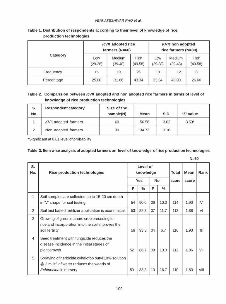
109
Table 1. Distribution of respondents according to their level of knowledge of rice production technologies
KVK adopted rice KVK non adopted farmers (N=60) rice farmers (N=30)
Low Medium High Low Medium High(29-38) (39-48) (49-58) (29-38) (39-48) (49-58)
Frequency 15 19 26 10 12 8
Percentage 25.00 31.66 43.34 33.34 40.00 26.66
Table 2. Comparision between KVK adopted and non adopted rice farmers in terms of level of knowledge of rice production technologies
S. Respondent category Size of theNo. sample(N) Mean S.D. ‘Z’ value
1. KVK adopted farmers 60 56.58 3.02 3.53*
2. Non adopted farmers 30 34.73 3.16
*Significant at 0.01 level of probability
Table 3. Item wise analysis of adopted farmers on level of knowledge of rice production technologies
N=60
S. Level ofNo. Rice production technologies knowledge Total Mean Rank
Yes No score score
F % F %
1 Soil samples are collected up to 15-20 cm depthin ‘V’ shape for soil testing 54 90.0 06 10.0 114 1.90 V
2 Soil test based fertilizer application is economical 53 88.3 07 11.7 113 1.88 VI
3 Growing of green manure crop preceding torice and incorporation into the soil improves thesoil fertility 56 93.3 04 6.7 116 1.93 III
4 Seed treatment with fungicide reduces thedisease incidence in the initial stages ofplant growth 52 86.7 08 13.3 112 1.86 VII
5 Spraying of herbicide cyhalofop butyl 10% solution@ 2 ml lt-1 of water reduces the weeds ofEchinocloa in nursery 50 83.3 10 16.7 110 1.83 VIII
Category
VENKATESHWAR RAO et al.
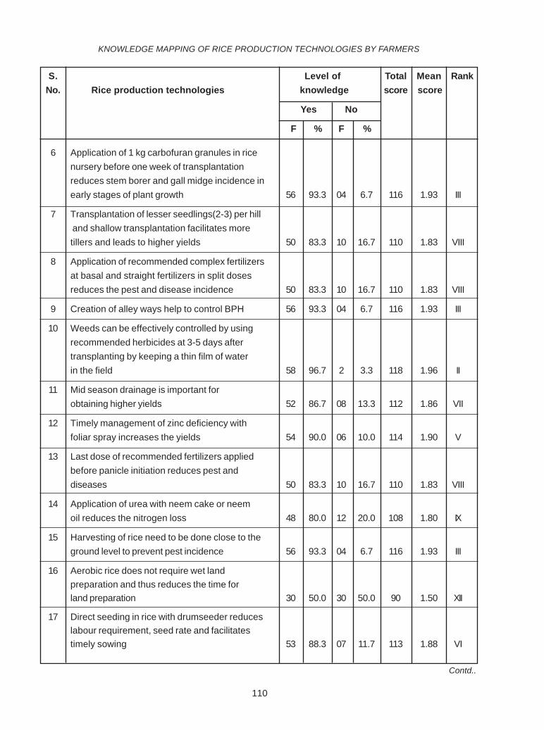
110
S. Level of Total Mean RankNo. Rice production technologies knowledge score score
Yes No
F % F %
6 Application of 1 kg carbofuran granules in ricenursery before one week of transplantationreduces stem borer and gall midge incidence inearly stages of plant growth 56 93.3 04 6.7 116 1.93 III
7 Transplantation of lesser seedlings(2-3) per hill and shallow transplantation facilitates moretillers and leads to higher yields 50 83.3 10 16.7 110 1.83 VIII
8 Application of recommended complex fertilizersat basal and straight fertilizers in split dosesreduces the pest and disease incidence 50 83.3 10 16.7 110 1.83 VIII
9 Creation of alley ways help to control BPH 56 93.3 04 6.7 116 1.93 III
10 Weeds can be effectively controlled by usingrecommended herbicides at 3-5 days aftertransplanting by keeping a thin film of waterin the field 58 96.7 2 3.3 118 1.96 II
11 Mid season drainage is important forobtaining higher yields 52 86.7 08 13.3 112 1.86 VII
12 Timely management of zinc deficiency withfoliar spray increases the yields 54 90.0 06 10.0 114 1.90 V
13 Last dose of recommended fertilizers appliedbefore panicle initiation reduces pest anddiseases 50 83.3 10 16.7 110 1.83 VIII
14 Application of urea with neem cake or neemoil reduces the nitrogen loss 48 80.0 12 20.0 108 1.80 IX
15 Harvesting of rice need to be done close to theground level to prevent pest incidence 56 93.3 04 6.7 116 1.93 III
16 Aerobic rice does not require wet landpreparation and thus reduces the time forland preparation 30 50.0 30 50.0 90 1.50 XII
17 Direct seeding in rice with drumseeder reduceslabour requirement, seed rate and facilitatestimely sowing 53 88.3 07 11.7 113 1.88 VI
Contd..
KNOWLEDGE MAPPING OF RICE PRODUCTION TECHNOLOGIES BY FARMERS

111
S. Level of Total Mean RankNo. Rice production technologies knowledge score score
Yes No
F % F %
18 Direct seeding in rice with drumseeder reducesthe crop period by 7-10 days and will alsoavoid one irrigation 53 88.3 07 11.7 113 1.88 VI
19 direct seeding in rice with drumseeder yieldsat par with normal transplantation 53 88.3 07 11.7 113 1.88 VI
20 In SRI high yields will be obtained with lowcost of cultivation and with low water consumption 50 83.3 10 16.7 110 1.83 VIII
21 Post emergence herbicide cyalofop butyl @400 ml acre-1 and ethoxy sulfuron @ 50 gm acre-1
spraying at 2-3 leaf stage of weeds willeffectively control all the weeds 45 75.0 15 25.0 105 1.75 X
22 Post emergence herbicide bispyribac sodium @120 ml acre-1 effectively controls both themonocots and broad leaved weeds 45 75.0 15 25.0 105 1.75 X
23 WGL -32100(Warangal Sannalu), a fine grainvariety has good cooking quality, will come toharvest 15 days early than BPT 5204 and giveshigher yield than BPT 5204 55 91.7 05 8.3 115 1.91 IV
24 NLR 34449, a fine grain variety has goodcooking quality and blast tolerance and giveshigher yield than BPT 5204 50 83.3 10 16.7 110 1.83 VIII
25 Low seed rate per acre with proper managementpractices will also give higher yields and resultin low cost of cultivation 50 83.3 10 16.7 110 1.83 VIII
26 Grain discolouration (panicle mite) will beeffectively controlled with prophylactic spray withprofenophos @ 400 ml and propiconazole@200 ml acre-1 before panicle emergence. 50 83.3 10 16.7 110 1.83 VIII
27 Hybrid seed production in rice gives higher netreturns compared to normal rice cultivation 60 100.0 0 0.0 120 2.00 I
28 Stem borer will be effectively controlled throughmass trapping with pheromone traps 40 66.7 20 33.3 100 1.66 X I
29 Seed production gives higher net returnscompared to normal rice cultivation 60 100.0 0 0.0 120 2.00 I
VENKATESHWAR RAO et al.

112
Table 4. Item wise analysis of non adopted farmers on level of knowledge of rice production technologies
N=60
S. Level of Total Mean RankNo. Rice production technologies knowledge score score
Yes No
F % F %
1 Soil samples are collected up to 15-20 cm depthin ‘V’ shape for soil testing 15 50.0 15 50.0 45 1.50 V
2 Soil test based fertilizer application is economical 15 50.0 15 50.0 45 1.50 V
3 Growing of green manure crop preceding to riceand incorporate into the soil improves thesoil fertility 22 73.3 08 26.7 52 1.73 II
4 Seed treatment with fungicide reduces thedisease incidence in the initial stages ofplant growth 18 60.0 12 40.0 48 1.60 IV
5 Spraying of herbicide cyhalofop butyl 10%solution @ 2 ml lt-1 of water reduces the weedsof echinocloa in nursery 15 50.0 15 50.0 45 1.50 V
6 Application of 1 kg carbofuran granules in ricenursery before one week of transplantationreduces stem borer and gall midge incidencein early stages of plant growth 15 50.0 15 50.0 45 1.50 V
7 Transplantation of lesser seedlings(2-3) per hilland shallow transplantation facilitates moretillers and leads to higher yields 18 60.0 12 40.0 48 1.60 IV
8 Application of recommended complex fertilizers atbasal and straight fertilizers in split dosesreduces the pest and disease incidence 20 66.7 10 33.3 50 1.66 III
9 Creation of alley ways help to control BPH 20 66.7 10 33.3 50 1.66 III
10 Weeds can be effectively controlled by usingrecommended herbicides at 3-5 days aftertransplanting by keeping a thin film of waterin the field 20 66.7 10 33.3 50 1.66 III
11 Mid season drainage is important for obtaininghigher yields 20 66.7 10 33.3 50 1.66 III
KNOWLEDGE MAPPING OF RICE PRODUCTION TECHNOLOGIES BY FARMERS

113
12 Timely management of zinc deficiency withfoliar spray increases the yields 20 66.7 10 33.3 50 1.66 III
13 Last dose of recommended fertilizers appliedbefore panicle initiation reduces pestand diseases 18 60.0 12 40.0 48 1.60 IV
14 Application of urea with neem cake or neemoil reduces the nitrogen loss 15 50.0 15 50.0 45 1.50 V
15 Harvesting of rice need to be done close tothe ground level to prevent pest incidence 20 66.7 10 33.3 50 1.66 III
16 Aerobic rice does not require wet landpreparation and thus reduces the time forland preparation 10 33.4 20 66.6 40 1.33 VI
17 Direct seeding in rice with drumseederreduces labour requirement, seed rate andfacilitates timely sowing 10 33.4 20 66.6 40 1.33 VI
18 Direct seeding in rice with drumseeder reducesthe crop period by 7-10 days and will alsoavoid one irrigation 10 33.4 20 66.6 40 1.33 VI
19 Direct seeding in rice with drumseeder yields atpar with normal transplantation 10 33.4 20 66.6 40 1.33 VI
20 In SRI, high yields will be obtained with lesscost of cultivation and less water consumption 10 33.4 20 66.6 40 1.33 VI
21 Post emergence herbicide cyalofop butyl@ 400 ml acre-1 and ethoxy sulfuron @ 50 gmacre-1 spraying at 2-3 leaf stage of weeds willeffectively control all the weeds 15 50.0 15 50.0 45 1.50 V
22 Post emergence herbicide bispyribac sodium@ 120 ml acre-1 effectively controls both themonocots and broad leaved weeds 15 50.0 15 50.0 45 1.50 V
23 WGL -32100(Warangal Sannalu) a fine grainvariety has good cooking quality will come toharvest 15 days lesser and gives higheryield than BPT 5204 20 66.7 10 33.3 50 1.66 III
S. Level of Total Mean RankNo. Rice production technologies knowledge score score
Yes No
F % F %
VENKATESHWAR RAO et al.

114
S. Level of Total Mean RankNo. Rice production technologies knowledge score score
Yes No
F % F %
24 NLR 34449 a fine grain variety has goodcooking quality will have blast tolerance andgives higher yield than BPT 5204 20 66.7 10 33.3 50 1.66 III
25 Lesser seed rate per acre with propermanagement practices will also give higheryields with lesser cost of cultivation 20 66.7 10 33.3 50 1.66 III
26 Grain discolouration (panicle mite) will effectivelycontrolled as prophylactic spray with profenophos@ 400 ml and propiconazole@ 200 ml acre-1
before panicle emergence 15 50.0 15 50.0 45 1.50 V
27 Hybrid seed production in rice gives higher netreturns compared to normal rice cultivation 25 83.3 5 16.7 55 1.83 I
28 Stem borer will be effectively controlled throughmass trapping with pheromone traps 15 50.0 15 50.0 45 1.50 V
29 Seed production in rice gives higher net returnscompared to normal rice cultivation 25 83.3 5 16.7 45 1.83 I
Table 3 indicates the item analysis of the KVKadopted farmers in rice crop on level of knowledgepossessed by them on rice technologies. It can benoted from Table 3 that ranks were assigned to alltechnologies based on the total score obtained oneach technology. The technologies on which therespondents had high level of knowledge are hybridrice and varietal seed production ranked 1st followedby weed management with recommendedherbicides(2nd ), green manuring to improve the soilfertility, application of carbofuran granules in nursery,creation of alley ways to control BPH (3rd rank),WGL 32100 a fine grain variety gives higher yieldthan BPT 5204 (4th ), method of soil sample collectionand timely management of zinc deficiency with foliarspray increases the yields (5th), soil test basedfertilizer application, direct seeding reduces seed
rate, labour requirement and crop period with lessercost of cultivation( 6th), seed treatment with fungicidereduces the disease incidence in the initial stagesof plant growth and mid season drainage is importantfor obtaining higher yields(7th), spraying of herbicidecyhalofop butyl 10% solution @ 2 ml lt-1 of waterreduces the weeds of echinocloa in nursery,transplantation of lesser seedlings(2-3) per hill andshallow transplantation facilitates more tillers leadsto higher yields, application of complex fertilizers atbasal and straight fertilizers in split up withrecommended doses reduces the pest and diseaseincidence, last dose of fertilizers applied beforepanicle initiation reduces pest and diseases, in SRIhigher yields will be obtained with lesser cost ofcultivation and with lesser water, NLR-34449 a finegrain variety has good cooking quality will have blast
KNOWLEDGE MAPPING OF RICE PRODUCTION TECHNOLOGIES BY FARMERS

115
tolerance and gives higher yield than BPT 5204,lesser seed rate per acre with proper managementpractices will also give higher yields with lesser costof cultivation and grain discolouration (Panicle mite)will effectively controlled as prophylactic spray withprofenophos @ 400 ml and propiconazole@ 200 mlacre-1 before panicle emergence ( 8th), application ofurea with neem cake or neem oil reduces the nitrogenloss (9th), post emergence herbicide cyalofop butyl@ 400 ml acre-1 and ethoxy sulfuron @ 50 gmacre-1 spraying at 2-3 leaf stage of weeds willeffectively control all the weeds, post emergenceherbicide bispyribac sodium @ 120 ml acre-1 willeffectively controls both the monocots and broadleaved weeds(10th), stem borer will be effectivelycontrolled through mass trapping with pheromonetraps (11th) and aerobic rice does not require wet landpreparation reduces the time for land preparation withlesser labour and lesser seed rate (12th), respectively.The KVK adopted farmers had lowest level ofknowledge on aerobic rice and mass trapping withpheromone traps will effectively controls stem borer.
In case of non adopted KVK farmers, thepractices such as hybrid rice and varietal seedproduction ranked 1st followed by green manuring toimproves the soil fertility (2nd), application of complexfertilizers at basal and straight fertilizers in split upwith recommended doses reduce the pest anddisease incidence, creation of alley ways to controlBPH, weed management by using recommendedherbicides, mid season drainage (3rd), seedtreatment, transplantation of lesser seedlings withshallow transplantation(4th), soil sample collection,soil test based fertil izer application, weedmanagement in nursery, usage of post emergenceherbicides(5th), direct seeding in rice reduces seedrate, labour requirement and lesser crop period withlesser cost of cultivation(6th), etc. The non adoptedKVK farmers had low level of knowledge on directseeding and SRI cultivation.
It is visible from the Table 1 that majority ofthe adopted rice farmers had high level of knowledgewhere as non adopted farmers had medium level ofknowledge. The item analysis of level of knowledgeof adopted rice farmers indicates that majority of themhad high knowledge on hybrid and varietal seedproduction followed by chemical weed management,improving soil fertility with green manures, BPHcontrol with the alleys, collecting the soil samples,soil test based fertilizer application, etc. The reasonsfor high level of knowledge on these technologiescould be suitability of the agro ecosystem ofKarimnagar district for hybrid and varietal seedproduction, as this was clearly envisaged by the KVKScientists to the rice farmers. Realising the ill effectsof continuous application of inorganic fertilizers, thefarmers were resorted to the application of greenmanures to improve the soil fertility. The continuousorganization of farmers field school, farmer – scientistinteractions, field days and focused groupdiscussions by the KVK scientists resulted information of alleys in rice crop to control the BPH,the farmers were experienced through a series ofmethod demonstrations conducted by KVKScientists on methods of collecting the soil samplesfor testing. The farmers were empowered andenriched on necessary competencies to apply theneed based fertilizers based on the results generatedfrom soil testing as it gives more economic returns.The adopted rice farmers had lowest level ofknowledge on aerobic rice due to non availability oftractor drawn seed cum ferti drill.
It could be witnessed from Table 4 that thenon adopted rice farmers had high level of knowledgeon hybrid and varietal seed production followed bygreen manuring for soil fertility, applying the complexfertilizers at basal and straight fertilizers in splitdoses, formation of alleys to control the BPH,chemical weed management, mid season drainage,seed treatment,etc. The non adopted rice farmers of
VENKATESHWAR RAO et al.
116
KVK are seldom inspired and motivated andinfluenced by the actions and deeds of their fellowadopted rice farmers. These non adopted farmerswant to replicate the successful practices carriedby the adopted farmers. Hence, the same level ofknowledge of adopted farmers on these technologiesis reflected in case of non adopted farmers also. Theseed of green manure crops is provided on subsidizedrate to the farmers by the government, hence moreknowledge. The non-adopted rice farmers had lowlevel of knowledge on direct seeding and SRIcultivation due to lack of interest, motivation andinspiration.
CONCLUSION
High level of knowledge of rice productiontechnologies was seen among the farmers adoptedby the KVK, Jammikunta compared to the nonadopted farmers. This could be due to the multiplicityof the transfer of technology mechanisms followedby the KVK scientists in the adopted villages
especially for the benefit of farmers adopted by theKVK.
REFERENCES
Balamatti, A.M., 1993. A study on rice cultivationpattern of Siddhi farmers and their socio-economic characteristics, Yellapur,Karnataka. M.Sc. Thesis submitted toUniversity of Agricultural Sciences,Dharwad.
Bhat, P.L. 1994. A study to identify the determinantsof yield gaps and constraints in ricecultivation of Jammu and Kashmir State.M.Sc. Thesis submitted to Andhra PradeshAgricultural University, Hyderabad.
Rao, N.V., Ratnakar, R and Jain, P.K., 2012. Impactof Farmer Field Schools in KVK adoptedvillages on level of knowledge and extent ofadoption of improved practices of rice. TheJournal of Research ANGRAU. XL(1) : 35-41.
KNOWLEDGE MAPPING OF RICE PRODUCTION TECHNOLOGIES BY FARMERS

117
Sex ratio is an important social indicator tomeasure the extent of equity between males andfemales in any society. In India, it has been observedthat mill ions of male population has beenoutnumbering the female population. The report of2011 Census of India shows 940 females per every1000 males (source: censusindia.gov.in). Accordingto Sen (1990), in countries where women and menreceive similar care the ratio is about 1005. Thisproblem of low sex ratio has further been aggravatedby low and the declining child sex ratio across allstates of India since 1961. Studies have providedevidence that it is excessive female mortality beforebirth, at birth, in infancy and in childhood, whichmainly account for the imbalance in sex ratios andmissing of large number female children( UNICEF,2014)This increasing gap between boys and girlsespecially in the age groups of 0-6 years gives us abetter picture of overall sex ratio and also the statusof girl child in Indian environment. The Northern andSouthern states exhibit considerable differences.While the north has lower levels of literacy and percapita income levels, the south generally exhibitshigher literacy levels, high percapita income levels,better health facilities and higher female participationrates. Studies have documented correlations of lowsex ratios at birth with higher education, social classand economic status. Objectives of the study are toexamine the trends in overall sex ratio and child sexratio across different states of India; to analyse theeffect of child sex ratio on overall sex ratio; to identifythe underlying causes of changes in child sex ratio
INTER TEMPORAL VARIATIONS IN SEX RATIO IN INDIA: STATE WISE ANALYSISP. KANAKA DURGA
National Institute of Agricultural Extension Management, Rajendranagar,Hyderabad – 500 030
Date of Receipt: 06.4.2017 Date of Acceptance:25.5.2017
J.Res. ANGRAU 45(2) 117-122, 2017
and overall sex ratio.Trends in overall sex ratio(OSR)and child sex ratio (CSR) and literacy levels areexamined across selected states of India with thehelp of various Census Reports. The data on percapita income is obtained from Economic Survey ofIndia (Source: www.indiastat.com). The followingregression models are specified to find out the effectof child sex ratio on overall sex ratio.
Model 1: OSRi = ¥1 +¥2CSRi + ui ——————1
Where OSR = overall sex ratio; CSR = Child sexratio; ¥1 and ¥2 are parameters
Model 2 : OSRi = 1 + 2 CSRi + 3 PIi + ui
Where OSR = overall sex ratio; CSR = child sexratio; PI = Percapita income; â1, â2,â3 areparameters
Trends in Sex Ratio: The low sex ratio before 1991was mainly due to the sex differentials in mortality(Visaria,1971). According to him, the contributionsof migration, under enumeration of females and sexratios at birth are having only a marginal influence.The overall sex ratio has shown a secular-decliningtrend except some marginal increases in thecensuses of 1951, 1981 and 2001. The sex ratio in2011 was 940, seven points higher than the sex ratioof 933 recorded in 2001. Although there was amarginal increase in general sex ratio at the nationallevel in 1981 and 2011, the child sex ratio has beencontinuously declining for the last five decades from976 in 1961 to 914 in 2011. It is observed that up to1991 the child sex ratio is more than overall sexratio. However, reversal of that trend can be observedfrom 2001 census onwards (Table 1).
Research Note
E-mail:[email protected]

118
Table 1. Sex Ratio in India
Census Year Overall Sex Ratio Child sex ratio Difference between( Females per (0-6 years) child sex ratio1000 Males) and overall sex ratio
1951 946 - -
1961 941 976 +35
1971 931 964 +33
1981 935 962 +27
1991 927 945 +18
2001 933 927 -06
2011 940 914 -26
Source: Office of the Registrar General and Census Commissioner, India
The child sex ratio is more than the overallsex ratio up to 1991. Between 1961 and 1991 thesupremacy of child sex ratio declined from 35 pointsto 18 points but still higher when compared to overallsex ratio. It was in the year 2001 that the child sexratio deteriorated and by 2011 there was a huge gapof 26 points. The child sex ratio has not only beenfalling but also from 2001 onwards it has been fallingshort of overall sex ratio and more steeply in 2011(Table 1). Socio-cultural discrimination against femalechildren is the main reason for female mortality mainly
because of life-sustaining inputs like food, nutrition,health care were denied to girl child (Miller, 1981).The overall sex ratio has exhibited a declining trendin all regions except in Northern and southern part ofthe country. In North India, the sex ratio is lowestand remained lowest throughout the period underconsideration. Maximum improvement in overall sexratio can be observed in north India followed by southIndia. In fact, in other regions the sex ratio has showna decline (Table 2).
Table 2. Overall Sex Ratio of Different Regions of India
Regions Census Year
South India 997 989 982 987 986 997 1010 13
North East India 966 941 920 918 921 940 959 -07
North India 768 785 801 808 827 821 866 98
East India 962 961 945 945 929 942 947 -15
Central India 985 970 959 959 949 955 961 -24
West India 985 962 939 943 936 931 934 -51
India 946 941 930 934 927 933 940 -06
Source: www.indiastat.com
Changebetween2011 and
19511951 1961 1971 1981 1991 2001 2011
KANAKA DURGA et al.

119
Child sex ratio is found to be highest in north easternregion in all the census years. Except north India,all other regions have exhibited declining trend withalmost same magnitude of change between 2011and 1991 (Table 3). Based on the spread of the datathe states are categorized into high, medium andlow levels of sex ratio. All four southern states fallunder the category of high sex ratio with regard tooverall sex ratio but with regard to child sex ratiothese states could not occupy the same category
except Kerala. Along with the southern states fournorth eastern states (Tripura, Mizoram, Meghalayaand Manipur) fall under the category of high sex ratiostates. This shows that the southern and northeastern states have been doing fairly well in terms ofoverall and child sex ratio when compared with otherstates. Almost all northern (Haryana, Punjab, UP,Jammu& Kashmir) and western states (Rajasthan,Maharastra, Gujarat) are under the category of lowsex ratio states (Table 4).
Table3.Child Sex Ratio (0-6 years of Age) in India : Region Wise
Change Regions Census Year between 2011
and 19911991 2001 2011
South India 960 954 948 -6North East India 978 969 956 -13North India 916 866 870 4East India 966 954 940 -14Central India 962 952 938 -14West India 938 909 896 -13India 945 927 914 -13
Source: Office of the Registrar General and Census Commissioner, India.
Table 4. Status of different states as per the overall Sex Ratio and Child Sex Ratio (2011 Census)
Overall Sex Ratio Child Sex Ratio
Status States Status States
High (above 960) AP*, Karnataka, Kerala, High Kerala, Arunachal Pradesh,Tamilnadu, Manipur, Meghalaya, (above 950) Assam, Meghalaya, Mizoram, Tripura, Himachal Mizoram, Tripura,Pradesh, Uttarakhand, Orissa, Chattisgarh, West BengalChattisgarh, Goa
Moderate Assam, West Bengal, Moderate AP, Karnataka, Tamilnadu,(between 960 Jharkand (between Manipur, Nagaland, Bihar,to 940) 950 to 914) Jharkand, Orissa, Goa
Low (below 940) Arunachal Pradesh Nagaland, Low Delhi, Haryana, HimachaHaryana, Jammu & Kashmir, UP, (below 914) Pradesh, Jammu & Kashmir,Punjab, Delhi, Bihar, MP, Gujarat, Punjab, UP, Uttarakhand,Maharastra, Rajasthan MP, Rajasthan,
Gujarat, Maharastra
*United AP
INTER TEMPORAL VARIATIONS IN POPULATION SEX RATIO IN INDIA

120
Table 5. Overall Sex Ratio of major states of India
ChangeRegion State 1991 2001 2011 Between 1991
and 2011
South India Andhra Pradesh 972 978 992 20
Karnataka 960 964 968 8
Kerala 1036 1058 1084 48
Tamil Nadu 974 986 995 21
North India Haryana 865 861 877 12
Punjab 882 874 893 11
Uttar Pradesh 876 898 908 32
East India Bihar 907 921 916 9
Orissa 971 972 978 7
West Bengal 917 934 947 30
West India Gujarat 934 921 918 -16
Maharashtra 934 922 925 -9
Rajasthan 910 922 926 16
Central India Madhya Pradesh 912 920 930 18
Source: Office of the Registrar General and Census Commissioner, India.
Among the southern states only Kerala achieved highest overall sex ratio and also highest improvementbetween 1991 to 2011. The least improved sex ratio state is Orissa during the same period (Table 5).
KANAKA DURGA et al.
With regard to child sex ratio almost all statesperformed low only with the exception of Kerala andTamilnadu. In these states, the child sex ratio isalmost constant between 1991 and 2011. The fall inchild sex ratio is very steep in western and northernstates (Table 6). There is hardly any state, whichhas child sex ratio of 1000 or more. It can be inferredthat the sex ratio imbalances are more severe in thenorth western region, which stretching fromUttaranchal in the north runs up to Maharastra in thewest across Himachal Pradesh, Punjab, Chandigarh,Haryana, Delhi, Rajasthan and Gujarat. This declinehas also been steep in the northern region. Kerala isthe only state recorded a favorable sex ratio forfemales. Many research works have been carriedout in finding out the answers for continuous fall insex ratio in India. Recent studies of female
infanticide, new biases in sex ratios at birth and infantand child mortality rates indicate that extreme formsof daughter discrimination resulting in death havepersisted (Miller, 1989). The hypotheses tested isthat as the child sex ratio declines, the overall sexratio also declines unless the health conditions ofthe adult females improves as a result of increase inincomes. This hypothesis is tested with the help oftwo models. Model 1 uses the change in child sexratio as independent variable and change in overallsex ratio as dependent variable.
The results of the Model 1 are as follows:OSRi = 33.965 +0.6549 CSRi
t value (3.34) R2 = 0.497
The results show that for every 10 pointsdecline in child sex ratio resulted in fall in overall
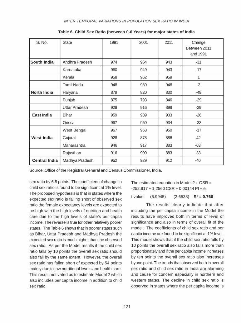
121
sex ratio by 6.5 points. The coefficient of change inchild sex ratio is found to be significant at 1% level.The proposed hypothesis is that in states where theexpected sex ratio is falling short of observed sexratio the female expectancy levels are expected tobe high with the high levels of nutrition and healthcare due to the high levels of state’s per capitaincome. The reverse is true for other relatively poorerstates. The Table 6 shows that in poorer states suchas Bihar, Uttar Pradesh and Madhya Pradesh theexpected sex ratio is much higher than the observedsex ratio. As per the Model results if the child sexratio falls by 10 points the overall sex ratio shouldalso fall by the same extent. However, the overallsex ratio has fallen short of expected by 54 pointsmainly due to low nutritional levels and health care.This result motivated us to estimate Model 2 whichalso includes per capita income in addition to childsex ratio.
The estimated equation in Model 2 : OSR =-252.917 + 1.2560 CSR + 0.00144 PI + ei
t value (5.9945) (2.6538) R2 = 0.766
The results clearly indicate that afterincluding the per capita income in the Model theresults have improved both in terms of level ofsignificance and also in terms of overall fit of themodel. The coefficients of child sex ratio and percapita income are found to be significant at 1% level.This model shows that if the child sex ratio falls by10 points the overall sex ratio also falls more thanproportionately and if the per capita income increasesby ten points the overall sex ratio also increasesbyone point. The trends that observed both in overallsex ratio and child sex ratio in India are alarmingand cause for concern especially in northern andwestern states. The decline in child sex ratio isobserved in states where the per capita income is
INTER TEMPORAL VARIATIONS IN POPULATION SEX RATIO IN INDIA
Table 6. Child Sex Ratio (between 0-6 Years) for major states of India
S. No. State 1991 2001 2011 ChangeBetween 2011
and 1991
South India Andhra Pradesh 974 964 943 -31
Karnataka 960 949 943 -17
Kerala 958 962 959 1
Tamil Nadu 948 939 946 -2
North India Haryana 879 820 830 -49
Punjab 875 793 846 -29
Uttar Pradesh 928 916 899 -29
East India Bihar 959 939 933 -26
Orissa 967 950 934 -33
West Bengal 967 963 950 -17
West India Gujarat 928 878 886 -42
Maharashtra 946 917 883 -63
Rajasthan 916 909 883 -33
Central India Madhya Pradesh 952 929 912 -40
Source: Office of the Registrar General and Census Commissioner, India.

122
KANAKA DURGA et al.
high which is a cause for concern and needsimmediate attention of policy makers and thegovernment.
REFERENCES
Censusofindia.2011. Sex ratio. Retreived from website( h t t p : / / c e n s u s i n d i a . g o v . i n /Census_Data_2001/India_at_glance/fsex.aspx on 30.3.2017).
Coale, A.J. 1991. Excess female mortality and thebalance of sexes in the population: Anestimated number of missing females.Population and development Review. 17(3):517-23.
Miller, B.D. 1981. The endangered sex. CornellUniversity Press, Ithaca, NewYork. pp.26-29.
Miller, B.D. 1989. Changing patterns of juvenile sexratios in rural India: 1961 to1971. Economicand Political Weekly. 24 (22): 1229-35.
Sen, A. 1992. Missing Women. British MedicalJournal.pp. 304.
Sen, A. 1990. More than 100 Million Women areMissing. New York Review of Books. pp. 61-66.
UNICEF.1995 .The State of World’s Children 1995Report. Oxford University Press publishedfor UNICEF. pp. 28-29.
UNICEF. 2014 .The State of World’s Children 2014in numbers: Every child counts Report.Newyork.pp.118-121.
Visaria, P. 1971. The sex ratio of the population ofIndia. Monograph 10, Census of India, NewDelhi: Office of the Registrar General, India.pp.36-38.

123
GUIDELINES FOR THE PREPARATION OF MANUSCRIPT
1. Title of the article should be short, specific, phrased to identify the content and indicate the nature ofstudy.
2. Names should be in uppercase prefixed with initials and separated by commas. For more than twoauthors the names should be followed by ‘and’ in lowercase before the end of last name. Full addressof the place of research in small letters should be typed below the names. E-mail i.d of the first author/ corresponding author may be given as foot note.
3. The full length paper should have the sub heads ABSTRACT, INTRODUCTION, MATERIAL ANDMETHODS, RESULTS AND DISCUSSION, CONCLUSION(S) and REFERENCES-all typed in uppercaseand bold font - 12. The research note will have only one sub head i.e. REFERENCES.
4. ABSTRACT: The content should include the year, purpose, methodology and salient findings of theresearch in brief not exceeding 200 words. It should be so arranged that the reader need not refer to thearticle except for details.
5. INTRODUCTION : Should be with title and indicate the reasons which prompted the research, objectivesand the likely implication. The review of recent literature should be pertinent to the problem. The contentmust be brief and precise.
6. MATERIAL AND METHODS : Should include very clearly the experimental techniques and the statisticalmethods adopted. Citation of standard work is sufficient for the well known methods.
7. RESULTS AND DISCUSSION : Great care should be taken to highlight the important findings withsupport of the data well distinguished by statistical measures like CD, r, Z test etc. Too descriptiveexplanation for the whole data is not desirable. The treatments should be briefly expressed instead ofabbreviations like T1, T2 , etc. The discussion should be concise and relate to the limitations or advantagesof the findings in comparision with the work of others.
8. REFERENCES : Literature cited should be latest. References dating back to more than 10 years arenot desirable. Names of authors, their spelling and year of publication should coincide both inthe text and references. The following examples should be followed while listing the references fromdifferent sources.
Journals and Bulletins
Abdul Salam, M and Mazrooe, S.A. 2007. Water requirement of maize (Zea mays L.) as influenced by
planting dates in Kuwait. Journal of Agrometeorology. 9 (1) : 34-41.
Hu, J., Yue, B and Vick, B.A. 2007. Integration of trap makers onto a sunflower SSR marker linkage mapconstructed from 92 recombinant inbred lines. Helia. 30 (46) :25-36.

124
Books
AOAC. 1990. Official methods of analysis. Association of official analytical chemists. 15th Edition. WashingtonDC. USA. pp. 256.
Federer, W.T. 1993. Statistical design and analysis for intercropping experiments. Volume I : Two Crops.Springer – Verlag, Cornell University, Ithaca, New York, USA. pp. 298-305.
Thesis
Ibrahim, F. 2007. Genetic variability for resistance to sorghum aphid (Melanaphis sacchari, Zentner) in sorghum.Ph.D. Thesis submitted to Acharya N.G. Ranga Agricultural University, Hyderabad.
Seminars / Symposia / Workshops
Naveen Kumar, P.G and Shaik Mohammad. 2007. Farming Systems approach – A way towards organicfarming. Paper presented at the National symposium on integrated farming systems and its role towardslivelihood improvement. Jaipur, 26 – 28 October, 2007. pp.43-46.
Proceedings of Seminars / Symposia
Bind, M and Howden, M. 2004. Challenges and opportunities for cropping systems in a changing climate.Proceedings of International crop science congress. Brisbane –Australia. 26 September – 1 October 2004.pp. 52-54. (website : www.cropscience 2004.com on 03-11-2004).
Tables and Graphs : The data in tables should not be duplicated in graphs and vice versa. Mean data formain treatment effects should be presented with appropriate SE± and CD values wherever necessary.The 2 or3 way tables should be furnished only if the results are consistent over years and aredistinguished to haveconsideration of significant practical value. SE± and CD values however,should be furnished in the tables forall interactions and should be explained in the results anddiscussion. The treatments should be mentionedatleast in short forms if they are lengthy, but not simply abbreviated as T1, T2 and T3, etc. The weights andmeasures should be given in the metric system following the latest units eg. kg ha–1, kg ha–1 cm, mg g–1, dSm–1, g m–3, C mol kg–1 etc.
Typing : The article should be typed in 12 pt font on A4 size paper leaving a margin of 2 cm on all sides.There should be a single line space between the rows in abstract and double line in rest. Verifythe manuscript thoroughly for errors before submitting it for publication.
Note : Latest issue of the Journal may be consulted. Further details can be obtained from the book“Editors Style Manual, Edition 4. American Institute of Biological Sciences, Washington DC”.
URL : http://www.angrau.ac.in/Publications
E-mail : [email protected]

125
THE JOURNAL OF RESEARCH ANGRAU
DECLARATION CERTIFICATE TO BE SUBMITTED BY THE AUTHOR(S)
Certified that the article entitled __________________________________________________________
____________________________________________________________________________________
1. is based on my / our original research work / M.Sc / Ph.D thesis (strike off whichever is not applicable)
2. The article has been seen by all the authors and the order of authorship is agreed.
3. The results presented have not been published or submitted for publication elsewhere in part or full underthe same or other title
4. The names of the authors are those who made a notable contribution.
5. No authorship is given to anyone who did not make a notable contribution.
S.No. Name/s Present address Permanent address Signature
1.
2.
3.
CERTIFICATE BY THE COMPETENT AUTHORITY
( Professor & Head of the Department/ Principal Scientist of the station/ Associate Director of Research).
Certified that the article ————————————————————————————————————
———————————————————————————————————————————————
authored by —————————————————————————————————————————
———————————————————————— is fit for publication. It fulfills all the requirements for
publication in The Journal of Research ANGRAU.
Name :
Signature :
Office seal :
Note: In case it is not possible to obtain the signature of a particular author for reasons beyondhis/her reach, the reasons thereof should be explained.

126
ESSENTIAL REQUIREMENTSFOR CONSIDERATION OF PUBLICATION OF ARTICLES
1. Research of not less than 2 years and of high standard will be considered as full length paper. Ifnecessary, it will be considered as Research Note.
2. M.Sc. Research of one year should be submitted in the style and format of Research Note.
3. The total number of pages should not exceed 10 for full paper and 5 pages for Research Note includingtables and figures.The figures should be legible.
4. Previous research of 5 years old before the date of submission will not be considered.
5. All the authors should subscribe for the Journal either as annual/life member.
6. The manuscript should be submitted (soft copy as e-mail) as per the guidelines of the Journal [email protected]
7. The manuscript should accompany the declaration certificate and subscription enrolment form(scannedsoft copy).
8. The authors should accept the editorial / reviwer comments until the quality of the paper is improved.
9. The revised manuscript should be submitted as a soft copy(e-mail) at [email protected]
10. Demand Draft may be drawn in favour of COMPTROLLER, ANGRAU, payable at Guntur.
SUBSCRIPTION TARIFF
ANNUAL
Individual : Rs. 300/- author
Institution : Rs. 1200/-
LIFEIndividual (till retirement) : Rs. 1200/-
1. Publications : Managing Editor - Journal of Research ANGRAU, Agricultural Information &CommunicationCentre,Guntur.The DD should be mailed to the Managing Editor,The Journal of Research ANGRAU,ESR ENCLAVE, BALAJI NAGAR, M.G. INNER RING ROAD, GUNTUR – 522 509.
Note : Latest issue of the Journal may be consulted. The weights and measures should be given in the metricsystem following the latest units eg. kg ha-1, kg ha-1 cm, mg g-1, dSm-1, g m-3, C mol kg-1 , etc.
Typing : The article should be typed in 12pt font on A4 size paper leaving a margin of 2 cm on all sides. Thereshould be a single line space between the rows in abstract and double line in rest.The article shallbe printed on only one side of paper.
URL : http://www.angrau.ac.in/publications
E-mail : [email protected]
127
SUBSCRIPTION ENROLLING FORM
I/we,herewith enclose D.D. No.....................................................................................................
dated ....................................for Rs. ............................... drawn in favour of COMPTROLLER, ANGRAU
payable at Guntur as individual annual/individual life/Institutional annual Membership for The Journal of Research
ANGRAU for the calendar year (January - December) ..................
S.No. Name of the Address for Name of the Signatureauthors correspondence article
1.
2.
3.
4.
Note: DDs shall be sent to Managing Editor, The Journal of Research ANGRAU, ESR Enclave,Balaji Nagar, M.G. Inner Ring Road, Guntur - 522 509.

128
Statement About The Ownership And Other Particulars About JournalTHE JOURNAL OF RESEARCH ANGRAU
Form IV (SEE RULE 8)
Place of Publication : Guntur
Periodicity of publication : Once in three months (Quarterly)
Printer’s Name : Ritunestham Press, Guntur
Nationality : INDIAN
Address : Ritunestham PressD.No. 8-198, Kornepadu, Guntur - 522 017
Publisher’s Name : Dr. R. Veeraraghavaiah
Address : Dean, P.G. Studies, Administrative Office,Acharya N.G. Ranga Agricultural University,Mahatma Gandhi Inner Ring Road,Guntur- 522 509, Andhra Pradesh
Editor’s Name : Dr. R.Veeraraghavaiah
Nationality : INDIAN
Address : Dean, P.G. Studies, Administrative Office,Acharya N.G. Ranga Agricultural University,Mahatma Gandhi Inner Ring Road,Guntur, - 522 509, Andhra Pradesh
Name and address of the individuals : Acharya N.G.Ranga Agricultural University,who own the newspaper and partners or Administrative Office,share holders holding more than one Mahatma Gandhi Inner Ring Road,percent of the total capital Guntur- 522 509, Andhra Pradesh.
I, Dr.R.Veeraraghavaiah, hereby declare that the particulars given above are true to the best of my knowledgeand belief
Date : 04.7.2017 Sd./-R.Veeraraghavaiah Signature of the Publisher

ANGRAU/July 2017 Regd. No. 25487/73
Printed at Ritunestham Press, Guntur and Published by Dr. R. Veeraraghavaiah, Dean, P.G. Studies and Editor,The Journal of Research ANGRAU, Acharya N.G. Ranga Agricultural University, Lam, Guntur - 522 034
E-mail : [email protected], www.angrau.ac.in/publications
THE JOURNAL OFRESEARCHANGRAU
ACHARYA N.G. RANGA AGRICULTURAL UNIVERSITY
Lam, Guntur - 522 034The J. Res. ANGRAU, Vol. XLV No. (2), pp 1-130, April-June, 2017
Indexed by CAB International (CABI)www.cabi.org and www.angrau.ac.in
The J. Res. A
NG
RA
U, Vol. XLV N
o. (2), pp 1-130, April-June, 2017
ISSN No. 0970-0226