1_descriptivo

Análisis multivariante en R: aplicación en ecología

Rosana Ferrero

5 de febrero de 2014

Índice

1. Análisis descriptivo de datos multivariantes con R 21.1. EJEMPLO EN R. . . . . . . . . . . . . . . . . . . . . . . . . . . . . . . . . . . . . . . . . . . . . 2

1

1. Análisis descriptivo de datos multivariantes con R

1.1. EJEMPLO EN R.

Este famoso conjunto de datos del iris (de Fisher o Anderson) da las medidas en centímetros de lalongitud de las variables sépalo y la anchura y la longitud y la anchura del pétalo, respectivamente, por 50flores de cada uno de 3 especies de iris. Las especies son setosa Iris, versicolor y virginica.

iris es una trama de datos con 150 casos (filas) y 5 variables (columnas) con nombre Sepal.Length,Sepal.Width, Petal.Length, Petal.Width, y especies.

data(iris) #abrimos el archivo de datos

# El archivo contiene un encabezado con los nombres de las variables# (header=T) y utiliza la comna como decimal (dec= , )head(iris)

## Sepal.Length Sepal.Width Petal.Length Petal.Width Species## 1 5.1 3.5 1.4 0.2 setosa## 2 4.9 3.0 1.4 0.2 setosa## 3 4.7 3.2 1.3 0.2 setosa## 4 4.6 3.1 1.5 0.2 setosa## 5 5.0 3.6 1.4 0.2 setosa## 6 5.4 3.9 1.7 0.4 setosa

tail(iris)

## Sepal.Length Sepal.Width Petal.Length Petal.Width Species## 145 6.7 3.3 5.7 2.5 virginica## 146 6.7 3.0 5.2 2.3 virginica## 147 6.3 2.5 5.0 1.9 virginica## 148 6.5 3.0 5.2 2.0 virginica## 149 6.2 3.4 5.4 2.3 virginica## 150 5.9 3.0 5.1 1.8 virginica

names(iris) #nombres de los datos

## [1] "Sepal.Length" "Sepal.Width" "Petal.Length" "Petal.Width"## [5] "Species"

str(iris)

## 'data.frame': 150 obs. of 5 variables:## $ Sepal.Length: num 5.1 4.9 4.7 4.6 5 5.4 4.6 5 4.4 4.9 ...## $ Sepal.Width : num 3.5 3 3.2 3.1 3.6 3.9 3.4 3.4 2.9 3.1 ...## $ Petal.Length: num 1.4 1.4 1.3 1.5 1.4 1.7 1.4 1.5 1.4 1.5 ...## $ Petal.Width : num 0.2 0.2 0.2 0.2 0.2 0.4 0.3 0.2 0.2 0.1 ...## $ Species : Factor w/ 3 levels "setosa","versicolor",..: 1 1 1 1 1 1 1 1 1 1 ...

# I. explorar cada variable por separado

# 1) variables cuantitativassummary(iris)

## Sepal.Length Sepal.Width Petal.Length Petal.Width

2

## Min. :4.30 Min. :2.00 Min. :1.00 Min. :0.1## 1st Qu.:5.10 1st Qu.:2.80 1st Qu.:1.60 1st Qu.:0.3## Median :5.80 Median :3.00 Median :4.35 Median :1.3## Mean :5.84 Mean :3.06 Mean :3.76 Mean :1.2## 3rd Qu.:6.40 3rd Qu.:3.30 3rd Qu.:5.10 3rd Qu.:1.8## Max. :7.90 Max. :4.40 Max. :6.90 Max. :2.5## Species## setosa :50## versicolor:50## virginica :50######

var(iris$Sepal.Length)

## [1] 0.6857

hist(iris$Sepal.Length)plot(density(iris$Sepal.Length))

Histogram of iris$Sepal.Length

iris$Sepal.Length

Fre

quen

cy

4 5 6 7 8

05

1015

2025

30

3

4 5 6 7 8

0.0

0.1

0.2

0.3

0.4

density.default(x = iris$Sepal.Length)

N = 150 Bandwidth = 0.2736

Den

sity

# 2) variables cualitativastable(iris$Species)

#### setosa versicolor virginica## 50 50 50

pie(table(iris$Species))barplot(table(iris$Species))

4

setosa

versicolor

virginica

5

setosa versicolor virginica

010

2030

4050

# II. explorar las variables en conjuntocov(iris[, 1:4])

## Sepal.Length Sepal.Width Petal.Length Petal.Width## Sepal.Length 0.68569 -0.04243 1.2743 0.5163## Sepal.Width -0.04243 0.18998 -0.3297 -0.1216## Petal.Length 1.27432 -0.32966 3.1163 1.2956## Petal.Width 0.51627 -0.12164 1.2956 0.5810

cor(iris[, 1:4])

## Sepal.Length Sepal.Width Petal.Length Petal.Width## Sepal.Length 1.0000 -0.1176 0.8718 0.8179## Sepal.Width -0.1176 1.0000 -0.4284 -0.3661## Petal.Length 0.8718 -0.4284 1.0000 0.9629## Petal.Width 0.8179 -0.3661 0.9629 1.0000

aggregate(Sepal.Length ~ Species, summary, data = iris)

## Species Sepal.Length.Min. Sepal.Length.1st Qu.## 1 setosa 4.30 4.80## 2 versicolor 4.90 5.60## 3 virginica 4.90 6.22## Sepal.Length.Median Sepal.Length.Mean Sepal.Length.3rd Qu.## 1 5.00 5.01 5.20## 2 5.90 5.94 6.30

6

## 3 6.50 6.59 6.90## Sepal.Length.Max.## 1 5.80## 2 7.00## 3 7.90

boxplot(Sepal.Length ~ Species, data = iris)with(iris, plot(Sepal.Length, Sepal.Width, col = Species, pch = as.numeric(Species)))plot(iris$Petal.Length, iris$Petal.Width, pch = 21, bg = c("red", "green3",

"blue")[unclass(iris$Species)], main = "Iris Data")pairs(iris[1:4], main = "Iris Data", pch = 21, bg = c("red", "green3",

"blue")[unclass(iris$Species)])


4.5

5.0

5.5

6.0

6.5

7.0

7.5

8.0

7

4.5 5.0 5.5 6.0 6.5 7.0 7.5 8.0

2.0

2.5

3.0

3.5

4.0

Sepal.Length

Sep

al.W

idth

8

1 2 3 4 5 6 7

0.5

1.0

1.5

2.0

2.5

Iris Data

iris$Petal.Length

iris$

Pet

al.W

idth

9

Sepal.Length

2.0 2.5 3.0 3.5 4.0 0.5 1.0 1.5 2.0 2.5

4.5

6.0

7.5

2.0

3.0

4.0

Sepal.Width

Petal.Length

13

57

4.5 5.5 6.5 7.5

0.5

1.5

2.5

1 2 3 4 5 6 7

Petal.Width

Iris Data

panel.cor <- function(x, y, digits = 2, prefix = "", cex.cor, ...) {usr <- par("usr")on.exit(par(usr))par(usr = c(0, 1, 0, 1))r <- abs(cor(x, y))txt <- format(c(r, 0.123456789), digits = digits)[1]txt <- paste(prefix, txt, sep = "")if (missing(cex.cor))

cex.cor <- 0.8/strwidth(txt)text(0.5, 0.5, txt, cex = cex.cor * r)

}pairs(iris[1:4], main = "Iris Data", pch = 21, bg = c("red", "green3",

"blue")[unclass(iris$Species)], upper.panel = panel.cor)

10

Sepal.Length

2.0 2.5 3.0 3.5 4.0

0.12 0.87

0.5 1.0 1.5 2.0 2.5

4.5

6.0

7.5

0.82

2.0

3.0

4.0

Sepal.Width 0.43 0.37

Petal.Length

13

57

0.96

4.5 5.5 6.5 7.5

0.5

1.5

2.5

1 2 3 4 5 6 7

Petal.Width

Iris Data

# gráficos 3Dlibrary(scatterplot3d)scatterplot3d(iris$Petal.Width, iris$Sepal.Length, iris$Sepal.Width)# library(rgl) plot3d(iris$Petal.Width, iris$Sepal.Length,# iris$Sepal.Width)

11

0.0 0.5 1.0 1.5 2.0 2.5

2.0

2.5

3.0

3.5

4.0

4.5

45

67

8

iris$Petal.Width

iris$

Sep

al.L

engt

h

iris$

Sep

al.W

idth

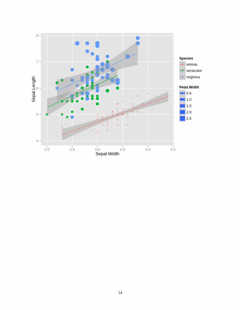
# gráficos más complejos: ggplot2library(ggplot2)qplot(Sepal.Length, Sepal.Width, data = iris, facets = Species ~ .)qplot(x = Sepal.Width, y = Sepal.Length, data = iris, geom = c("point",

"smooth"), color = Species, size = Petal.Width, method = "lm")qplot(x = Sepal.Width, y = Sepal.Length, data = iris, geom = c("point",

"smooth"), color = Species, size = Petal.Width, method = "lm", facets = ~Species)qplot(x = Sepal.Width, y = Sepal.Length, data = iris, geom = c("point",

"smooth"), color = Species, size = Petal.Width, method = "lm", facets = Species ~.)

12

2.0

2.5

3.0

3.5

4.0

4.5

2.0

2.5

3.0

3.5

4.0

4.5

2.0

2.5

3.0

3.5

4.0

4.5

setosaversicolor

virginica

5 6 7 8Sepal.Length

Sep

al.W

idth

13

4

5

6

7

8

2.0 2.5 3.0 3.5 4.0 4.5Sepal.Width

Sep

al.L

engt

h

Species

setosa

versicolor

virginica

Petal.Width

0.5

1.0

1.5

2.0

2.5

14


4

5

6

7

8

2.0 2.5 3.0 3.5 4.0 4.52.0 2.5 3.0 3.5 4.0 4.52.0 2.5 3.0 3.5 4.0 4.5Sepal.Width

Sep

al.L

engt

h

Species

setosa

versicolor

virginica

Petal.Width

0.5

1.0

1.5

2.0

2.5

15

4

5

6

7

8

4

5

6

7

8

4

5

6

7

8

setosaversicolor

virginica

2.0 2.5 3.0 3.5 4.0 4.5Sepal.Width

Sep

al.L

engt

h

Species

setosa

versicolor

virginica

Petal.Width

0.5

1.0

1.5

2.0

2.5

# gráficos más complejos: ggplot2library(reshape2)iris$flower_id <- rownames(iris)

iris_melted <- melt(iris)

## Using Species, flower_id as id variables

head(iris_melted)

## Species flower_id variable value## 1 setosa 1 Sepal.Length 5.1## 2 setosa 2 Sepal.Length 4.9## 3 setosa 3 Sepal.Length 4.7## 4 setosa 4 Sepal.Length 4.6## 5 setosa 5 Sepal.Length 5.0## 6 setosa 6 Sepal.Length 5.4

split_variable <- strsplit(as.character(iris_melted$variable), split = "\\.")iris_melted$flower_part <- sapply(split_variable, "[", 1)iris_melted$measurement_type <- sapply(split_variable, "[", 2)iris_melted$variable <- NULLhead(iris_melted)

## Species flower_id value flower_part measurement_type## 1 setosa 1 5.1 Sepal Length

16

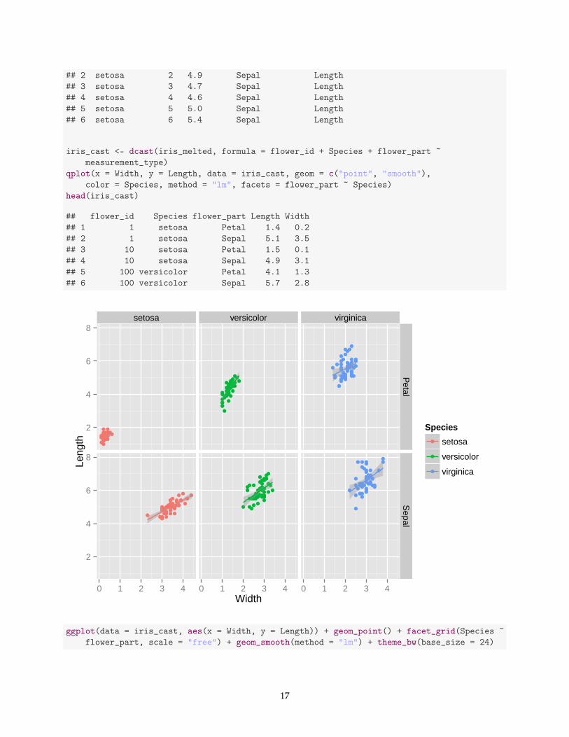
## 2 setosa 2 4.9 Sepal Length## 3 setosa 3 4.7 Sepal Length## 4 setosa 4 4.6 Sepal Length## 5 setosa 5 5.0 Sepal Length## 6 setosa 6 5.4 Sepal Length

iris_cast <- dcast(iris_melted, formula = flower_id + Species + flower_part ~measurement_type)

qplot(x = Width, y = Length, data = iris_cast, geom = c("point", "smooth"),color = Species, method = "lm", facets = flower_part ~ Species)

head(iris_cast)

## flower_id Species flower_part Length Width## 1 1 setosa Petal 1.4 0.2## 2 1 setosa Sepal 5.1 3.5## 3 10 setosa Petal 1.5 0.1## 4 10 setosa Sepal 4.9 3.1## 5 100 versicolor Petal 4.1 1.3## 6 100 versicolor Sepal 5.7 2.8


2

4

6

8

2

4

6

8

Petal

Sepal

0 1 2 3 4 0 1 2 3 4 0 1 2 3 4Width

Leng

th

Species

setosa

versicolor

virginica

ggplot(data = iris_cast, aes(x = Width, y = Length)) + geom_point() + facet_grid(Species ~flower_part, scale = "free") + geom_smooth(method = "lm") + theme_bw(base_size = 24)

17

Petal Sepal

123456

34567

5678

setosaversicolor

virginica

0.0 0.5 1.0 1.5 2.0 2.52.0 2.5 3.0 3.5 4.0 4.5Width

Leng

th

my_plot <- ggplot(data = iris_cast, aes(x = Width, y = Length, shape = flower_part,color = flower_part)) + geom_point() + facet_grid(~Species) + geom_smooth(method = "lm")

my_plot

18


2

4

6

8

0 1 2 3 4 0 1 2 3 4 0 1 2 3 4Width

Leng

th

flower_part

Petal

Sepal

library(ggthemes)my_plot + theme_excel(base_size = 24)my_plot + theme_wsj(base_size = 18)

19


2

4

6

8

0 1 2 3 4 0 1 2 3 4 0 1 2 3 4Width

Leng

th

flower_part

Petal

Sepal

20


2

4

6

8

0 1 2 3 4 0 1 2 3 4 0 1 2 3 4

flower_part Petal Sepal

Fuente de algunos gráficos: https://github.com/raphg/Biostat-578/blob/master/AdvancedgraphicsinR.Rpres

21

1_descriptivo

Documents

Transcript of 1_descriptivo