Bearings By Andre Lam (18) Lau Wai Soong (19) Ivan Leo (20) Lim Bing Wen (21) Triangle Trigonometry.
8/4/2019 1992 Lim Vibration Sea Bearings
http://slidepdf.com/reader/full/1992-lim-vibration-sea-bearings 1/14
Journal of Sound and Vibration (1992) 153(l), 37-50
V I BR A T I O N T R A N SM I SS I O N T H R O U G H R O LLI NG ELEM EN T
BEARING S , PART IV: ST ATIST ICAL ENERGY ANALYSIS
T. C. LIM? AND R. SINGH
Department of Mechanical Engineering, 7he Ohio Stat e Univ ersity , 206 W est 18th Avenue,
Columbus, Ohio 43210-1107, U.S.A.
(Received 6 December 1989, and accepted in revised form 7 January 1991)
A theoretical coupling loss factor for the vibration transmission through a rolling element
bearing problem has been developed for the statistical energy analysis (SEA ) technique.This scheme includes the bearing stiffness matrix developed earlier in the companionpaper Part I. The same problem has been analyzed previously by using deterministic
vibration mod els in Parts II and III. In this pap er, a new analytical proc edure is develo ped
to obtain the coupling loss factor between the shaft and casing w hich is based on thesolution of the boundary value problem at the plate-bearing interface. Several example
cases are chosen to demonstrate the salient features of this method: I, a plate-cantilevered
beam problem; II, case I with circular shaft-bearing replacing the cantilevered beam; III,a shaft-bearing-plate system. Exam ple case I is a revised version of the problem analyzed
earlier by Lyon and Eichler (reference [6] of this paper). Our proposed calculation indicatesan improve ment in the coupling loss facto r prediction for a thin plate-cantileve red beam
system. Exam ple case II deals with the development of a theoretical scheme to compute
coupling loss factor for a bearing system. This development is extended further to predictmean-square vibratory response of a rectangular plate for example case III. Results ofthe statistical energy analysis comp are well with the predictions yielded by deterministic
model of Part II. Predictions for example cases I and III are found to be in good agreem entwith m easurements.
1. INTRODUCTION
It has been show n in Parts I-III [l-3], by using classical lumped parameter and dynamic
finite element (FEM ) techniques, that the proposed bearing model is clearly superior to
the existing simple models for predicting vibration transmission through bearings in a
shaft-bearing-plate system. Although the proposed models have been shown to be reliableup to a moderately high frequency, it is conceivable that these models are inadequate at
very high frequencies where the modal density tends to be high. Classical vibration models
do not predict modes accurately in this frequency regime, and even if it is possible to do
so by employing closely spaced nodal points, such models require a significantly large
computational effort. Moreover, the vast amount of predicted response spectra at many
spatial points w ould be difficult to interpret. Accordingly, asymptotic or statistical m ethods
must be adopted; typical techniques include the statistical energy analysis [4-81,
asymptotic modal analysis [9-111 and asymptotic analysis using infinite system imped-
ances [12].
This study is concentrated on the development of a theoretical broadba nd coupling
loss factor, which is a key parameter for the statistical energy a nalysis (SEA), of a
shaft-bearing-plate system. The SEA method has been applied successfully to those
structural and acoustic systems which exhibit high modal overlap and weak coupling
t Currently with Structural Dynamics Research Corporation, Milford, Ohio 4515 0, U.S.A.
37
0022460X /92/040037 + 14 %03.00/O @ 1992 Academic Press Limited

8/4/2019 1992 Lim Vibration Sea Bearings
http://slidepdf.com/reader/full/1992-lim-vibration-sea-bearings 2/14
38 T. C. LIM AND R. SINGH
between subsystems [4-8, 13-181 . However several unresolved research issues still exist
[5,8-10,19,20]. The specific objectives of this study are (i) to develop a theoretical
scheme to compute a coupling loss factor for a typical rolling element bearing system,
(ii) to demonstrate the applicability of SEA to the bearing problem, (iii) to analyze the
following three example cases: I, a plate-cantilevered rectangular beam; II, case I with
circular shaft-bearing system replacing the cantilevered beam; III, a circular shaft-
bearing-plate-mount system; and finally, (iv), to perform parametric studies to examine
the characteristics of vibratory energy transfer through bearings. The first and second
example cases are revised a nd extended versions of a study performed by Lyon and
Eichler [4,6]. The final example case examines an experimental set-up which was analyzed
earlier in Part II [2] by using the deterministic finite element method. Predictions yielded
by each method will be compared with the experimental results.
2. LITERATU RE REVIEW
A majority of publications are on the application of SEA to dynamic systems with high
modal overlap a nd weak coupling such as structural-acoustical interactions in a fuselage
[4,13,21], interior noise predictions [ 131, and vibratory energy transmission in mechan ical
equipme nt [4]. Of interest here is analytical or experimental estimation of SEA parameters
for simple structural systems described by a flat plate, a cylinder and/or a shaft [4,6,7, 141.
In these studies, structural connections are often assum ed rigid such as in the ideally
welded case.
Lyon and Eichler [4,6] in 1964 and Lyon and Scharton [7] in 1965 developed analytical
expressions for the coupling loss factor n in several connected structures, such as a plate
bonded to a cantilevered beam [4,6]. Here 71 was derived by assum ing a semi-infinite
beam attached to an infinite plate an d by further assum ing that only a dynamic mom ent
coupling at the joint can describe the motion/force transmission phenomenon. This
problem is re-examined in this study and is then extended to a circular shaft-bearing-
plate-mount system. In addition. Lyon and Eichler [4,6] also developed SEA models of
two structures inter-connected through a single (scalar) stiffness element. Typical examples
include two discrete masse s coupled by a linear spring, and a plate attached to a
single-degree-of-freedom resonator [4]. The longitudinal vibration of linearly coupled
rods was analyzed by Remington and M anning [18] in 1975 . Loss factors of typical line
or point connected structures such as a plate welded to a cylinder, cross-beams and two
perpendicular plates bolted or welded together have been calculated assum ing ideal rigid
joints [4, 6, 7, 22, 231. But a compliant bearing support problem is yet to be analyzed.
3. EXAMPLE CASE I: COUPLING LOSS FACTOR OF PLATE-CANTILEVERED BEAM
SYSTEM
First, we attempt to rework the plate-cantilevered beam problem of Lyon and Eichler
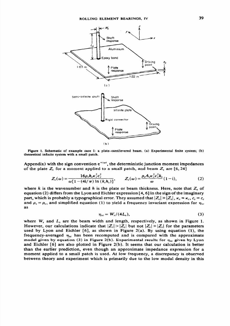
[4,6] as shown in Figure 1. Only flexural motions of the rectangular plate and rectangular
beam are considered in this case. Accordingly, Lyon and Eichler [4 ,6] developed an
expression for the coupling loss factor n sCwhich describes the vibratory energy transfer
between the beam(s) and the plate(c) due to a mom ent coupling at the joint,
(1 )
where K, = m is the radius of gyration, c, = m is the wave speed, m, is the ma ss
and Re ( ) implies the real part of a complex variable (a list of symbols is given in the
8/4/2019 1992 Lim Vibration Sea Bearings
http://slidepdf.com/reader/full/1992-lim-vibration-sea-bearings 3/14
ROLLING ELEMEN T BEARINGS, IV 39
Shaftresponse
Semi-infinite shaft Shaftresponse
Figure 1. Schem atic of example case I: a plate-cantilevered beam. (a) Experim ental finite system; (b)
theoretical infinite system with a small patch.
Appendix) with the sign convention e+‘“‘, the deterministic junction mom ent impedancesof the plate 2, for a mom ent applied to a small patch, and beam 2, are [6,24]
16p,h,&f
zc(~)=o[I-(4i/?r)ln(k,h,~)]’Z,(w) =
~,A,;:c:k, (I _ i),(2 )
where k is the wavenumber and h is the plate or beam thickness. Here, note that 2, of
equation (2) differs from the Lyon and Eichler expression [4,6] in the sign of the imaginary
part, which is probably a typographical error. They assumed that ]Z,] >> ZS], K, = K,, c , = cc
and pS = pe, and simplified equation (1 ) to yield a frequency invariant expression for qSC
as
77X W/(4&), (3)
where W , and L, are the beam width and length, respectively, as shown in Figure 1.
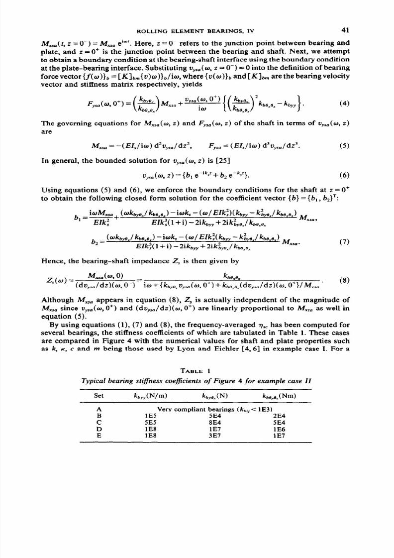
However, our calculations indicate that IZ,] > ]Z,] but not ]Z,] >> Z,l for the param eters
used by Lyon and Eichler [6], as shown in Figure 2(a). By using equation (l), the
frequency-averaged T,, has been recomputed and is compared with the approximate
model given by equation (3) in Figure 2(b). Experimental results for vSCgiven by Lyonand Eichler [6] are also plotted in Figure 2(b). It seems that our calculation is better
than the earlier prediction, even though an approximate impedance expression for a
mom ent applied to a small patch is used. At low frequency, a discrepancy is observed
between theory and experiment which is primarily due to the low modal density in this

8/4/2019 1992 Lim Vibration Sea Bearings
http://slidepdf.com/reader/full/1992-lim-vibration-sea-bearings 4/14
40 T. C. LIM AND R. SINGH
I .0 ____-__-_ __ ______ -_-______ _
;‘.~1 , I,,,,,
loo locc
Frequency (Hz)
- Low modal
z - density
b < It I,D A
I
g 10-Z: I
s _-----r &f____ ------ -_-----_--__D IrEa I *u I n *
A h
L L) ,
,o -3 (b) i , I I II,,,
102 103
One-third octave band center frequency (Hz)
Figure 2. Comp arison between the Lyon and Eichler approximation [4,6] and our propose d formulation
for example case I. (a) Com parison of ]Z,]/]Z, +Z,]; - - -, approximate mode l; -, proposed . (b) Com parisonof predicted qsc with experimen tal results given by Lyon and Eichier [4,6]; A, experim ent; -, least squares
curve fit of experimental data; -, proposed ; - - -, approximate mode l.
regime. The presence of a low natural frequency may be due to the compliant epoxy
bond between the beam and plate. However, above the threshold frequency where many
modes participate, shown as a vertical line in Figure 2(b), the slope of the least squares
straight line fit on the experimental data is nearly the same as the predicted v,,.
4. EXAMPLE CASE II: COUPLING LOSS FACTOR OF CIRCULAR SHAFT-BEARING-
PLATE SYSTEM
Next, we modify Figure 1 by inserting a ball bearing between the circular shaft (which
replaces the rectangular beam in Figure 1) and the rectangular plate. Aga in, a semi-infiniteshaft and an infinite plate are assum ed. For SEA , we reduce the system to a plate subsystem
and a shaft-bearing subsystem. The coupling loss factor T,, is still given by equation (l),
but 2, must be modified to account for the compliant bearing.
Consider a shaft with boundary conditions shown in Figure 3. The bearing end is
subjected to zero transverse velocity u ,,~~(, z = O-) = 0 and a sinusoidally varying mom ent
1-+alSemi - lnfmte shaft
Figure 3. Boundary conditions fo r example ca se II: semi-infinite shaft-bearing system.
8/4/2019 1992 Lim Vibration Sea Bearings
http://slidepdf.com/reader/full/1992-lim-vibration-sea-bearings 5/14
ROLLING ELEMENT BEARINGS, IV 41
A4,,,( f, 2 = 0) = M,,, e’“‘. Here, z = O- refers to the junction point between bearing and
plate, and z = O+ is the junction point between the bearing and shaft. Next, we attempt
to obtain a boundary condition at the bearing-shaft interface using the boundary condition
at the plate-bearing interface. Substituting u,,,,( o, z = O-) = 0 into the definition of bearing
forcevector {f(w)}b = [K]bm{u)~)} / io, where {u(o)}* and [ Klb,,, are the bearing velocity
vector and stiffness matrix respectively, yields
(4)
The governing equations for MX so(o, z) and Fyso(o, z) of the shaft in terms of 2)yso(o,)
are
M ,,, = -( EIJiw) d*v,,,f dz2, F,,, = (El&) d3uys./dz3. (5)
In general, the bounded solution for t)ys.(o, z) is [25]
vysa(w,z) = {b, epik”+ b2 e-“ s’}.
Using equations (5) and (6), we enforce the boundary conditions for the shaft at z = O+
to obtain the following closed form solution for the coefficient vector {b} = {b, , b2}T:
iwM,,,b,=s+
(wkbye,/bexex)iwk - (w/ EIkf)(kb,, k2b,exlbxex). .
s E I k z ( 1+ 1) - Zlk,,,, + 2 i k i y O x /k b O x O xM x.30,
b _ (~kbyex/kb~x~x) iwk -(w/E%(kb,, - kiye,/k,oxox) M2-
EIk:( 1+ i) - 2ikbYyt-2 ik & +/ k b O x O x X S a ’ (7)
Hence, the bearing-shaft impedance 2, is then given by
MxsAw, ) k Q 9,
z(w)= (duy, , / W(w , 0 - j = iw + {kbye ,uysah 0 ’ ) f kb , , (duy, , / dz) (w , 0+) /M , , , *
(8 )
Although M,, , appears in equation (8), 2, is actually independent of the magnitude of
M,, , since +(w, O+) and (du,,,/dz)(w, O+) are linearly propo rtional to M,, , as well in
equation (5).
By using equations (l), (7) and (8), the frequency-averaged n,, has been computed forseveral bearings, the stiffness coefficients of which are tabulated in Table 1. These cases
are compared in Figure 4 with the numerical values for shaft and plate properties such
as k, K, c and m being those used by Lyon and Eichler [4,6] in example case I. For a
TABLE 1
Ty pica l bearing s t i$ness coef ic ien t s o f Figure 4 for exam ple case I I
Set
AB
C
DE
h&N/m) kbyq(N) k,,,_(Nm)
Very compliant bearings (k,, < lE3)lE5 SE4 2E4
5E5 8E4 SE4lE8 lE7 lE6lE8 3E7 lE7
8/4/2019 1992 Lim Vibration Sea Bearings
http://slidepdf.com/reader/full/1992-lim-vibration-sea-bearings 6/14
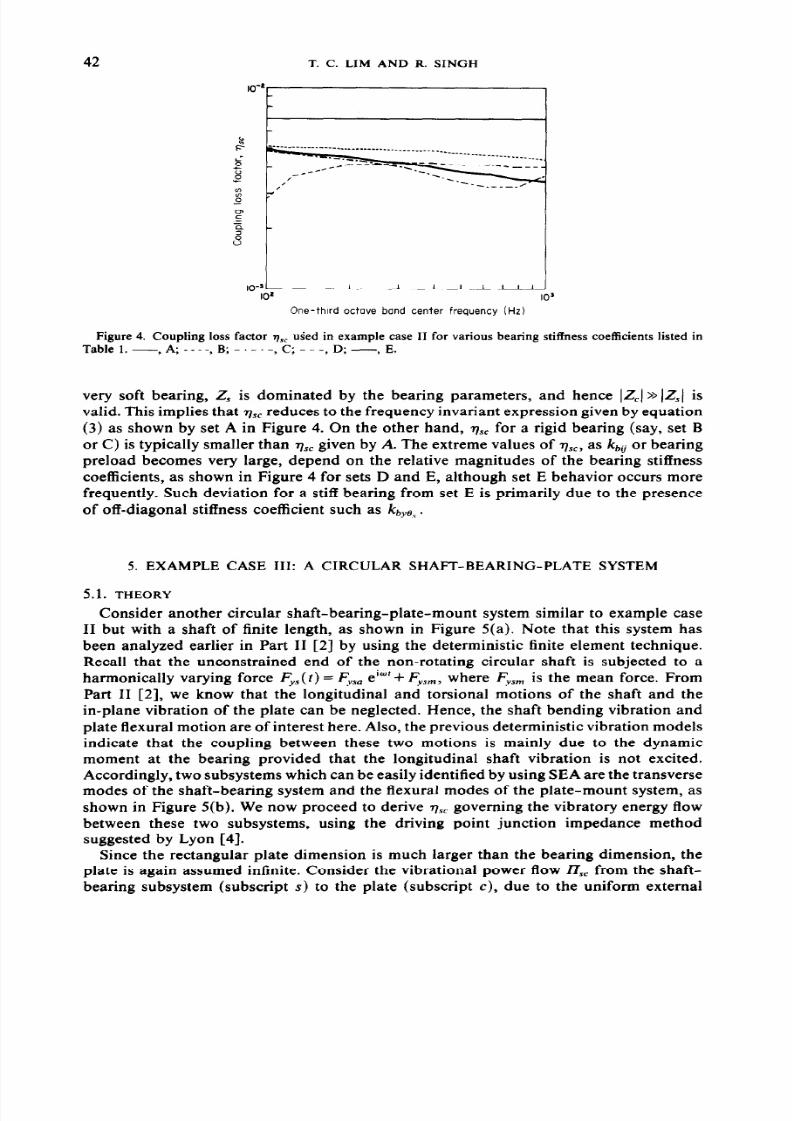
42 T. C. LIM AND R. SINGH
10-a I 1 1 I1 II1
IO' IO'
One- th rd oc tave band cen te r f requency (Hz)
Figure 4. Coup ling loss factor v,~ uSed in exam ple case II for various bearing stiffness coefficients listed inTablel.-,A;----,B;-.-.-,C;---,D;-,E.
very soft bearing, 2, is dominated by the bearing parameters, and hence lZ,l>> JZ,( is
valid. This implies that n ,, reduces to the frequency invariant expression given by equation
(3) as shown by set A in Figure 4 . On the other hand, q,, for a rigid bearing (say, set B
or C) is typically smaller than nlscgiven by A. The extreme values of nsc, as kbiior bearing
preload becomes very large, depend on the relative m agnitudes of the bearing stiffness
coefficients, as show n in Figure 4 for sets D and E, although set E behavior occurs more
frequently. Such deviation for a stiff bearing from set E is primarily due to the presenceof off-diagonal stiffness coefficient such as kby,, .
5. EXAMPLE CASE HI: A CIRCULAR SHAFT-BEARING-PLATE SYSTEM
5.1. THEORY
Consider another circular shaft-bearing-plate-mount system similar to example case
II but with a shaft of finite length, as shown in Figure 5(a). Note that this system has
been analyzed earlier in Part II [2] by using the deterministic finite element technique.
Recall that the unconstrained end of the non-rotating circular shaft is subjected to aharmonically varying force F,,(t) = F;,, eiwt+ F;,,, where F,,, is the mean force. From
Part II [2], we know that the longitudinal and torsional motions of the shaft and the
in-plane vibration of the plate can be neglected. Hence, the shaft bending vibration and
plate flexural motion are of interest here. Also, the previous deterministic vibration models
indicate that the coupling between these two motions is mainly due to the dynamic
mom ent at the bearing provided that the longitudinal shaft vibration is not excited.
Accordingly, two subsystems which can be easily identified by using SEA are the transverse
modes of the shaft-bearing system and the flexural modes of the plate-mount system, as
shown in Figure 5(b). We now proceed to derive nsc governing the vibratory energy flow
between these two subsystems, using the driving point junction impedance methodsuggested by Lyon [4].
Since the rectangular plate dimension is much larger than the bearing dimension, the
plate is again assumed infinite. C onsider the vibrational power flow 17,, from the shaft-
bearing subsystem (subscript s) to the plate (subscript c), due to the uniform external

8/4/2019 1992 Lim Vibration Sea Bearings
http://slidepdf.com/reader/full/1992-lim-vibration-sea-bearings 7/14
ROLLING ELEMENT BEARINGS, IV 43
‘“\G-x(a)
- - --> Energy diss ipatkm
I
l a te -mount sys tem qr
( f lexuml modes )
t
----> Energy i s s ipa t ion
E,(w), n,(w)
(b )
Figure 5. Exam ple case III: (a) schema tic of the circular shaft-bearing-plate-mount system described in
references [2,26] and (b) SEA model of the physical system.
Gaussian random force over a frequency bandwidth do with center frequency w,
where nj and E’ (j = s, c) refer to subsystem modal density and total vibratory energy
respectively. The modal densities per Hz of a shaft n, and rectangular plate n,, given for
bending motion with simply supported boundary conditions [4], are
n, = L,?p,?rd~/4EIsw2, n,=A,lh,J3p,(l-C12)lE, (10)
where p is the material density, A, is the plate surface area, L, is the shaft length, E is
the modulus of elasticity, I, is the area moment of inertia of the shaft, o is the bandwidth
center frequency, h, is the plate thickness, d, is the shaft diameter, p is the Poisson ratio,
and the subscripts s and c denote the shaft and the plate respectively. Since the plate is
assumed to be reasonably well damped and geometrically large, equation (9) is approxi-
mated assuming n, >> , or EC/n, +c Es/n, to yield
n,,(o) =Rc(~)I~Es(~). (11)
For the shaft, Es = m,( Vz), where m, is the shaft ma ss and (Vz) is mean square shaft

8/4/2019 1992 Lim Vibration Sea Bearings
http://slidepdf.com/reader/full/1992-lim-vibration-sea-bearings 8/14

8/4/2019 1992 Lim Vibration Sea Bearings
http://slidepdf.com/reader/full/1992-lim-vibration-sea-bearings 9/14
ROLLING ELEMENT BEARINGS, IV
Th e non-zero elements of coefficient matrix [B] of dimension 4 are
45
B,,=Lw
Elk: - i k b,,, + B,*=lik 2
0-EIkz-ik,,,,,,+3
k b& %
B,,=i‘(
k 2Elk : - kby y+ -
k, B,,=i
k 2
w-Elk:-k,,,+-
bW % W k h e,
B2, = B22=-B23=-B24=1, B3,=-1B41=le ,-iksLs
BS2=1Bd2=-le ,ik,L,
k L
B,, = -B ,, = -e- 1 5,k L
B34= Bu=e 5 I. (16)
Both [B] and {b} = {b, , b2, b, , b,}T can be easily obtained numerically. The bearing-shaft
impedance 2, is still given by equation (8).
The same procedure may be applied to obtain the driving point force impedance for
a harmonically varying transverse force F,,,( t, z = 0). Note that the origin is redefined atthe forcing point, as shown in Figure 6(b) for convenience. The boundary conditions are
E,,,(w,z=O)=E,,,, &= (w, z =O ) = 0, t)ys,(w, z = -L;) = 0 and (du,,,/dz)(w, -J!J = 0.
In a manner similar to that of the previous analysis, one obtains
k&(W , z = -Ls) = -{kbexer du , ,Jdz ) (w , - t z )+ kby e ,Vpa(w , -L f ) )/ (iw ) ,
Fys a(w , Z = -LS) = -{kby ex(doy , ,/dx ) (w , -L :)+kby y$sa(w , -L t ) )/ (iw ) . (17)
These prescribed boundary conditions again yield a set of algebraic p roblem similar to
equation (15). The non-zero elements of the coefficient matrix [B] of dimension 4 are
83, = (- ik ,k b, , i - k , ,, + Elk s) e ik JLs, B32 = ( ikS k bexex k , ,, - I-EZk f ) e - ik*Ls ,
BgJ = (- k ,kb, , + k by e,- Elk :) ekS 4, B34 = ( kS k bexex k b , , - E lk f ) e -ksLs ,
BJ1 = ( ik ,k , ,, - k b, ,, , iElk :) e iks LA , B42 = (- ik ,kb, , - kb,,, ,+ i EIk: ) eS iksLs ,
B a = ( k s k b y e , k b y y+ Elk :) ek sL *, B u = ( -k s k b y e , - k b, ,, - EIk z ) eeksL *. (18)
The right-hand side vector {b} of the algebraic problem is (0, F,, ,w /(EIk ~), 0 , O }T. The
force impedance at the driving point is then given by Z,(w, z = 0) = Fysa/u,_,(w, 0).
Accordingly, the input power is J7, = (1/2)F$, Re {(l/Z,)*} where Re { } is the real part
of the complex variable and ( )* implies complex conjugation. .
We can now compute the vibratory energy transfer & through the bearing and the
steady state subsystem energy levels ES an d EC by applying the energy balances to both
subsystems shown in Figure 5 (b); here TJ,,= n,,n,/ n, :
Es(w)=a(% + %s)
J%(W)17 %
w(775%%%c+ 77*% 1’ w W I, + %%c+ rlsr)cs 1.(20)
Since E = m ( V’), the following velocity levels may be obtained at any center frequency

8/4/2019 1992 Lim Vibration Sea Bearings
http://slidepdf.com/reader/full/1992-lim-vibration-sea-bearings 10/14
46 T. C. LIM AND R. SINGH
-15010 0 1000 10000
One- th i rd oc tave band cen te r f requency (Hz)
Figure 7. Compariosn between theory ( ) and experiment [26] (0) for example case III with a finiteshaft. Here plate mobility level in dB is 10 log,, ( V:) re ( Vz) = I.0 (m/s)’ for F,,, = 1 O N.
One- th i rd oc tave band cen te r f requency (Hz)
Figure 8. Comparison between theory ( )for a semi-infinite shaft.
and experiment [26] (0) for example case III. Here theory is
10-C
tIO-” . * * a ’ . ’ .
0 5000 IO
Frequency (Hz)
Figure 9.case HI.
Predicted co upling loss factor 7)s~ or a semi-infinite (-) and a finite shaft (-) shaft in exam ple

8/4/2019 1992 Lim Vibration Sea Bearings
http://slidepdf.com/reader/full/1992-lim-vibration-sea-bearings 11/14
ROLLING ELEMENT BEARINGS, IV 41
o from either equation (19) or (20):
(21)
5.2. VALIDATION AND PARAMETRIC STUDIES
In order to validate our SEA formulation, we compare the mean square mobility level
of the plate with experimental data provided by reference [26] as reported earlier in Part
II [2]. Note that although all non-zero bearing stiffness coefficients kbti were computed
and given in Part II [2], only k,,, = 3.69E8, kb,,,X= 3.52E5 and k b O X O X4*19E4 are used
as they appear to be the most significant ones according to the proposed theory. By using
equation (20), (Vz) has been computed, and is compared with experimental results in
Figure 7. Theoretical predictions for three values of frequency-invariant dissipation loss
factor 7, = 7, are given since the choice of structural damping seems to be critical for
SEA . It can be seen from Figure 7 that the experimental data are approximately boundedby v5 = O-0003 and v5 = 0.03, w hich are typical values for a lightly damp ed structure. It
is possible that 75 and vE vary with frequency in the experiment; this is not included in
our calculations. Accordingly, the agreement between theory and experiment is deemed
to be excellent.
Further comparison between theory and experiment can be made for the case of a
semi-infinite shaft considered in the example case II. By using equations (l), (7) and (8)
for 7),,, the mobility levels were computed and found to be given by straight lines, as
shown in Figure 8. These lines represent the asymptotic behavior of the system when the
shaft is very long: i.e., L, + co. Again , most experimental data are bounded within the
range given by n5 = 0*0003 to 0.03. Next consider the finite shaft length L , = 1.32 m ofhigh modal density n,. In Figure 9 the coupling loss factor Q, for this compared with
the result for a semi-infinite shaft. It can be seen that nsC or the semi-infinite shaft follows
the frequency -averaged values of the finite shaft. Finally, plate mobility leve ls predicted
by SEA for these two cases are compared in Table 2 with the results yielded by the
deterministic finite element model of Part II. Here, a nominal dissipation loss factor
7)s= rlr = 0.003 w as chosen for calculations. It is evident that S EA is indeed applicable
for this physical system.
TABLE 2
Com par ison o f resu l t s for exam ple case I I I
Plate mobility level (dB re( V2),P,= 1 O m2/ N2s2)
One-third octave Deterministic SEA predictionband center Experiment FEM method ,
frequency (Hz) WI P I Finite shaft Semi-infinite shaft
400 -102 -105 -102 -89500 -92 -96 -87 -9163 0 -95 -94 -90 -93
800 -88 -97 -93 -951000 -87 -95 -97 -971250 -97 -108 -101 -1001600 -108 -115 -106 -1042000 -106 -107 -112 -106

8/4/2019 1992 Lim Vibration Sea Bearings
http://slidepdf.com/reader/full/1992-lim-vibration-sea-bearings 12/14
48 T. C. LIM AND R. SINGH
6. CONCLUDING REMARKS
The vibration transm ission through a bearing in a generic shaft-bearing-plate system
has been analyzed by using the SEA technique. A new theoretical procedure has been
developed to compute the frequency-averaged coupling loss factor which relies on the
solution of the boundary value problem at the plate-bearing interface. This scheme
incorporates the rolling element bearing stiffness matrix developed earlier as a part of
the deterministic vibration models in the compan ion papers Parts I-III [l-3]. The
proposed formulation has been applied to a physical set-up consisting of a shaft canti-
levered to a plate through a bearing support. The vibratory response of the rectangular
plate predicted by SEA has been found to be in good agreement with measurem ents and
with the results of the deterministic models of Part II. There are still several unresolved
issues which require further research. For example, a more precise analysis of the mom ent
applied to a plate through a beam in example case I is required. Improved estimation
procedures for damping associated with bearing systems are needed. Perhaps of more
importance is the extension of proposed methodology to rotating m achinery noise and
vibration problems. In fact, work is in progress with application to the gearboxes.
ACKNOWLEDGMENT
We wish to thank the NASA L ewis Research Center for supporting this research at
The Ohio State University, and J. S. Lin and D. R. Houser for providing the experimental
data of case III.
REFERENCES
1. T. C. LIM and R. SINGH 1990 Journnl ofSound and Vibration 139(2), 179-199. Vibrationtransmission throu gh rolling element bearings, part I: bearing stiffness formulation.
2. T. C. L IM and R. SINGH 1990 Journal ofSound and Vibration 139(Z), 201-225. Vibration
transmission throu gh rolling element bearings, pa rt II: system studies.3. T. C. LIM and R. SINGH 1991 Journal of Sound and Vibration 151(l), 31-54. Vibration
transmission through rolling element bearings, part III: geared rotor system studies.4. R. H. LYON 1975 Statistical Energy Analysis of Dynamical Systems. Cambridge, Massachusetts:
The MIT Press.5. J. WOODHOUSE 1981 Applied Acoustics 14, 455-469. An introduction to statistical energ y
analysis of structural vibration.6. R. H. LYON and E. EICHLER 1964 Journalof th e Acous t i ca l Society of America 36(7), 1344-1354.
Random vibration of connected structures.7. R. H. LYON and T. D. SCHARTON 1965 Journal of the Acoustical Society of America 38(2),
253-261. Vibrat ional-energy transmission in a three -eleme nt structure.
8. R. S. LANGLEY 1989 Journal of Sound and Vibration 135,499-508. A general derivation of the
statistical energy analysis equations for coupled dynamic systems.9. E. H. DOWELL and Y. KUBOTA 1985 Journal of Applied Mechnics 52, 949-957. Asymptotic
mod al analysis and statistical energy analysis of dynamical system s.10. Y. KUBOTA and E. H. DOWELL 1986 Joumulof Sound and Vibration 106,203-216. Experimental
investigation of asymptotic modal analysis for a rectangular plate.11. Y. KUBOTA, H. D. DIONNE and E. H. DOWELL 1988 Journal of Vibration, Acoustics, Stress,
and Reliability in Design 110,371-37 6. Asymptotic modal analysis and statistical energy analysisof an acoustic cavity.
12. E.SKUDRZYK 1980 Journal of the Acoustical Society of America 67(4), 1105-1135. The
mean-value method of predicting the dynamic response of complex vibrators.13. V. R. MILL ER 1980 M.S. I l resis, The Ohio State University. Prediction of interior noise by
statistical energy analysis (SEA) method.14. B. L. CLARKSON and K. T. BROWN 1985 Journal of Vibration, Acoustics, Stress, and Reliability
in Design 107, 357-360. Acoustic radiation damping.

8/4/2019 1992 Lim Vibration Sea Bearings
http://slidepdf.com/reader/full/1992-lim-vibration-sea-bearings 13/14
ROLLING ELEMENT BEARINGS, IV 49
15. J. C. SUN, H. B. SUN, L. C. CH OW and E. J. RICHAR DS 1986JournalofSound and Vibration
104 ,243-257.Predict ionsof tot al loss facto rs of structures, art I I : loss facto rs of sand-fi l led
structure.
16. G. J. STIMP SON, J. C. SUN and E. J. RIC HAR DS 1 986Journal of Sound and Vibration 107,
107-120. Predicting sound pow er radiation from built-up structures using statistical energyanalysis.
17. A. J. KEANE and W. G. PRICE 1987 ournal ofSound and Vibration 117, 363-386. Statistical
energy analysis of strongly coupled systems.18. P. J. REMI NGTON and J. E. MANNING 197 5 ournalo f the Acoustical Society of America 57(2),
374-379. Com parison of statistical energy analysis po wer flow predictions with an “exact”calculation.
19. J. WOODHOUSE 1981 ournalof theAcousticalSocieryofAmericn 69(6), 1695-1709. An approach
to the theoretical background of statistical energy analysis applied to structual vibration.20 . P. W. SMITH, JR. 1979Journalof the Acoustical Society of America 65(3), 695-698. Statistical
models of coupled dynamical systems and the transition from weak to strong coupling.21. G. P. MATH UR, J. E. MANNING and A. C. AUBERT 1988NO ISE-CON 88, Purdue University ,
W est Lafayette. Bell 222 helicop ter cabin noise: analytical modeling and flight test validation.22. J. L. GUYADER , C. BOISSON and C. LESUEUR 198 2 ournal of Sound and Vibration 81, 81-92.
Energy transm ission in finite couple d plates, p art 1: theory .23. W. L. GHERING and D. RAJ 1987 Proceedings of the W inter Annual Meeting of the Am erican
Society of Mechnicul Engineers, Bost on, 81-90. Comparison of statistical energy analysis predic-
tions with experimental results for cylinder-plate-beam structures.24. I. DYER 1960 ournalof the AcousficulSocietyofAmericu 32( lo), 1290-1296. Moment impedance
of plates.25. L. CREMER, M. HECKEL and E. E. UNGAR 1973 Structure-Borne Sound. Berlin: Springer-
Verlag.26 . J. S. LIN 1989M.S. Thesis, The Ohio Stat e University. Experimental analysis of dynamic fo rce
transmissibility throu gh bearings.
APPENDIX: LIST OF SYMB OLS
plate surface areashaft cross-sectional area
wave speed
flexural rigidity of the shafttotal vibratory energy level in the shaft-bearing (s) subsystem and plate (c) subsystem
applied alternating shear force on the shaftapplied mean sh ear force on the shaft
bearing force vectorplate thicknessproposed bearing stiffness matrix of dimension 6
bearing stiRtress coefficient, i, j = x, y , z , S,, 0,,, Brshaft (s) or plate (c) wavenumbershaft lengthalternating shaft bending mom ent about x direction
plate massshaft mass
plate modal densityshaft modal density
real part of a complex numbertimespatially and frequency bandwidth averaged mean square mobilityalternating shaft tranverse velocity
bearing velocity vectordriving point plate impeda nce at bearing junctiondriving point sha ft impe dance at bearing junctiondriving point shaft impedance at forcing locationdissipation loss factor for the shaft-bearing (s) or plate (c) subsystemscoupling loss factor

8/4/2019 1992 Lim Vibration Sea Bearings
http://slidepdf.com/reader/full/1992-lim-vibration-sea-bearings 14/14
5 0 T. C. LIM AND R. SING H
radius of gyration
;; external pow er input to the shaft-bearing (s) subsystem
ZC net pow er transfer from the shaft-bearing (s) subsystem to plate (c) subsystems
P material density
bandwidth center frequency
Y,* complex conjugate