CONTROL APPLICATIONS USING NEURAL NETWORKS

by

Barton Earl Showalter

S. B., Massachusetts Institute of Technology

(1987)

SUBMITTED TO THE DEPARTMENT OF AERONAUTICS AND ASTRONAUTICS

IN PARTIAL FULFILLMENT OF THE REQUIREMENTS FOR THE

DEGREE OF MASTER OF SCIENCE

at the

MASSACHUSETTS INSTITUTE OF TECHNOLOGY

September, 1988

Signature of Author

'-I~~~~~~- &- ,"Department of Aeronautics and Astronautics/vL,? .

Approved byN\J

A

Certified by

William D. GoldenthalTechnical Supervisor, CSDL

Professor Wallace E. VanderVeldeThesis Supervisor

Accepted by,..,. --- -Professor Harold Y. Wachman/-z'J i_.k .. _ 'li.k --'uiental Graduate Committee

WP 07 188! W1TH '*fa V'

'I 3 M.. T'

' -~0'1- 3-,: .''it th

w~~ I - S

- "

CONTROL APPLICATIONS USING NEURAL NETWORKS

by

Barton Earl Showalter

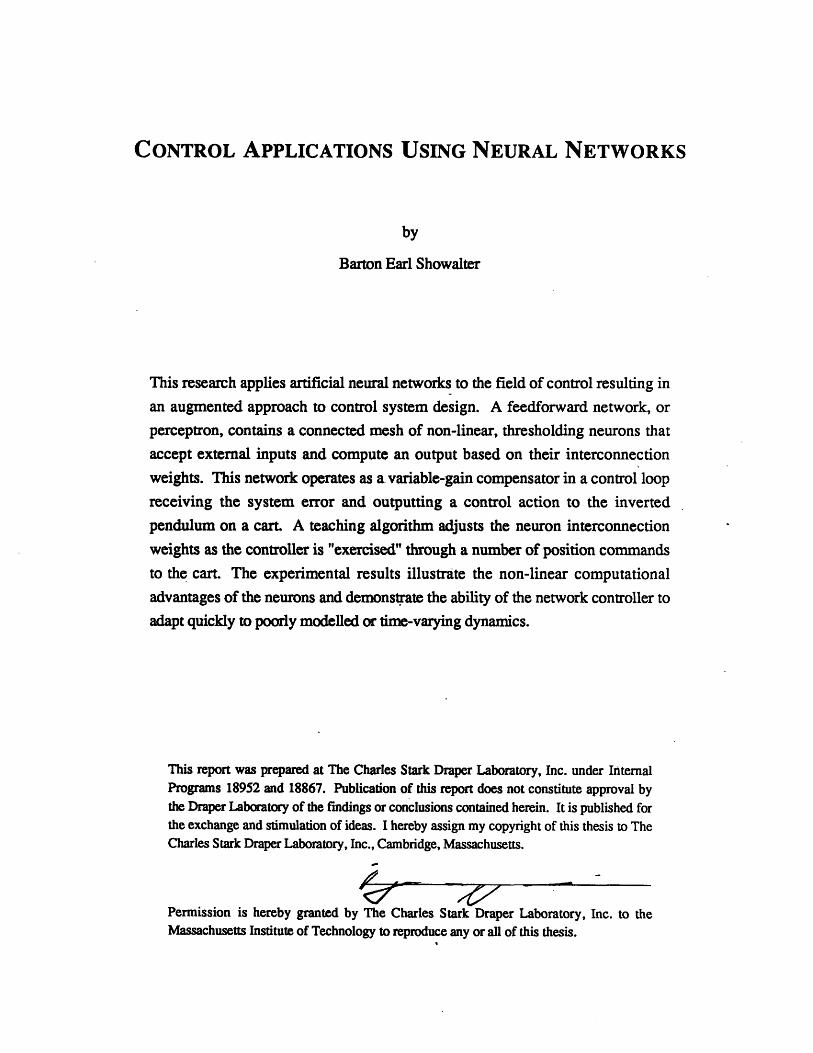
This research applies artificial neural networks to the field of control resulting in

an augmented approach to control system design. A feedforward network, or

perceptron, contains a connected mesh of non-linear, thresholding neurons that

accept external inputs and compute an output based on their interconnection

weights. This network operates as a variable-gain compensator in a control loop

receiving the system error and outputting a control action to the inverted

pendulum on a cart. A teaching algorithm adjusts the neuron interconnection

weights as the controller is "exercised" through a number of position commands

to the cart. The experimental results illustrate the non-linear computational

advantages of the neurons and demonstrate the ability of the network controller to

adapt quickly to poorly modelled or time-varying dynamics.

This report was prepared at The Charles Stark Draper Laboratory, Inc. under InternalPrograms 18952 and 18867. Publication of this report does not constitute approval bythe Draper Laboratory of the findings or conclusions contained herein. It is published forthe exchange and stimulation of ideas. I hereby assign my copyright of this thesis to TheCharles Stark Draper Laboratory, Inc., Cambridge, Massachusetts.

Permission is hereby granted by The Charles Stark Draper Laboratory, Inc. to theMassachusetts Institute of Technology to reproduce any or all of this thesis.

TABLE OF CONTENTS

1 INTRODUCTION 1

1.1 The History of Neural Networks ................. 1

1.2 Advantages of Neural Networks ..................... 3........ .. .... 3

1.3 Control Applications ................................................................ 3

2 PERCEPTRONS 5

2.1 Neurons ................... 5...............................................

2.1.1 Summation Function ................... 6...............................6

2.1.2 Output Function ........... 6................. ... ..6

2.2 Perceptron Substructure ........................... 82.3 The Perceptron as a Controller . . ......................................... 9

2.4 Network Propagation ................ ........... ................. ........ 112.4.1 Complete Propagation ....................... ..... .. .... 122.4.2 One-Step Propagation . ........................................ 12

2.5 Teaching ........................................................................... 12

3 NETWORK TEACHING STRATEGIES 15

3.1 The Neural Network as a Controller ............................. 15

3.2 Teaching Neural Networks Using Error Propagation .. .......... 16

3.2.1 The Lesson .............................................................. 17

3.2.2 Learning Rate and Momentum ....................................... 17

3.2.3 Periodic Updating ........................................ ........ ....... 173.2.4 Weight Initialization .................................................... 17

3.3 Backpropagation ...... 18

3.3.1 Teaching Controllers Using Backpropagation ....................... 18

3.3.2 Applying Backpropagation ............................................ 19

3.4 Forpropagation .................................................................... 203.4.1 Teaching Controllers Using Forpropagation ........................ 20

3.4.2 Applying Forpropagation .............................................. 21

4 THE PLANT 23

4.1 Problem Definition ............................................................... 234.2 Equations of Motion ............................................................. 24

5 THE REFERENCE 27

5.1 Need for the Reference ........................................................... 27

5.2 Background on Model Reference .... ........................... 285.2.1 Initial Information ....................................................... 285.2.2 System Reset ............................................................ 28

5.2.3 State Variables to Track ................................................. 29

Tracking Only Cart Position and Velocity ......... ........ 29

Tracking All State Variables ........................................... 30

5.2.4 Weight Update Interval . ............................... 305.2.5 Weight Update Test ................................ 30

5.3 Design of the Reference .......................................................... 31

6 THE NETWORK 33

6.1 The Network Control Loop .................................... 336.1.1 Variable Definitions ..................................................... 336.1.2 The Neural Network .................................................... 346.1.3 The Plant .............................................................. 34

6.1.4 The Gain Matrices ..................................................... 35

6.2 Operation of the Network Control Loop ......................... 35

6.3 Controller Architectures ................... ................... 6.................6.3.1 The Full-State Pole Position Controller .............................. 37

Classical Control Technique ........................................... 37

Analogous Network Controller .. 39

6.3.2 The Full-State Cart Position Controller .............................. 39

Classical Control Technique .40

Analogous Network Controller ....................................... 42

7 THE ADAPTER 44

7.1 The Forpropagation Control Loop .. .................................... 44

7.2 Operation of the Adapter ......................................................... 45

7.3 Forpropagation Algorithm Derivation . ........................ 46

7.3.1 Gradient Descent ........................................................ 47

7.3.2 The Neuron Error ....................................................... 48

The Dynamic Sign ...................................................... 49

The Propagation Term ................................. 50Final Expression for the Neuron Error ............................... 52

7.3.3 Weight Change Equation.................................52

8 IMPLEMENTATION 5 4

8.1 Neural-Network-Controller............. ............ .......................... 54

8.2 Pole-Exec .................................................. ....... 568.3 Forprop ............................................................................ 57

8.4 Pole-Dynamics ..................... 58

8.5 Big-Graph ................... ................... .. ......... ... 59

9 EXPERIMENTAL RESULTS 60

9.1 The Classical Controller ......................................................... 609.2 The Neural Network Controller ................................................. 63

9.3 Summary of the Results ................................ 74

10 RECOMMENDATIONS AND CONCLUSIONS 78

10.1 Conclusions ................ 8......................................... 78

10.2 Recommendations for Further Work ........................................... 79

10.2.1 Partial-State Feedback Controllers .................................... 80

10.2.2 Adjustable Reference ................................................... 81

APPENDIX 82

A. 1 Pole-exec.lisp ..................................................................... 82

A.2 Forprop.lisp ........... ...... 91

A.3 Pole-dynamics.lisp ................. ....................... ..... 103

REFERENCES 112

ACKNOWLEDGEMENTS

I owe a special thanks to Professor Wally VanderVelde, my thesis supervisor, for

his technical guidance and patience. I hope he has learned something about neural

networks through our friendly association.

Thanks also to my friends at C. S. Draper Laboratory, especially the basketball

crew, to whom I apologize again for not playing in the big game. Many thanks to Bill

Goldenthal, my technical supervisor, who approached me with an exciting thesis topic and

allowed me to pursue some original ideas. I am also indebted to Jim Cervantes, the Lisp

guru, for hours of free-lance hacking and software consulting that somehow brought the

Neural Network Controller to fruition. Another rising star on the Symbolics, Doug

Eberman, also provided me with a nice graphing package and overall software support.

As for general sounding block and MacYahtzee companion, that distinction must go

to my officemate and Texas-Ex, Walter Baker. The "can I erase this?" board, Speed

Reversi, and afternoon outings with Gambi will be greatly missed.

Thanks to Carol, Ifeanyi and the kids for being my family in Boston. Finally,

thanks to Mom, Dad, and the sibs for all their long-distance support during my five year

vacation at MIT.

To My Wife

LIST OF SYMBOLS

E error between actual and commanded plant state

f(netj) neuron output function at the value of netj

f '(netj) slope of the neuron output function at the value of net

F control force on cart (N)

g gravity (9.8 m/sec2)

G 1 gain matrix for network inputs

G2 gain matrix for network outputs

K1, K2 gains on the classical controller Xloop

K3, K4 gains on the classical controller 0 loop

L pole length (m)

L' effective pole length (m)

M cart mass (kg)

m pole mass (kg)

Mp percent overshoot

net vector containing all neuron internal states

netj sum of the weighted inputs or internal state of neuron j

o vector containing all neuron external states

oj ' output or external state of neuronj

Pik propagation term from neuron i to output neuron k

Pkk propagation term for output neuron k

R residual between actual plant state and model reference state

Rh residual of input neuron h

s Laplace operator

tj target output of neuron j

u network input vector

U plant input vector containing control commands

UM model reference vector containing target plant control commands

wij connection weight from neuron i to neuron j

Awij(P+ 1) current connection weight change

Awij(p) previous connection weight change

X cart position (m)

Xc commanded cart position

X cart velocity (m/sec)

Xc commanded cart velocity

X cart acceleration (m/sec2 )

y network output vector

Y plant output vector containing state variables

YD desired state of the plant

YM model reference vector containing target plant state

Si error of neuron j(h)ji error of neuron j for the residual input h

E£ scalar adaptive error

co damping coefficient of classical controller 8 loop

damping coefficient of classical controller Xloop

r/ learning coefficient

0 pole position (rad)

0c commanded pole position

0 pole velocity (rad/sec)

0c commanded pole velocity

9 pole acceleration (rad/sec2)

A constant determining steepness of the sigmoid function

14 momentum coefficient

Pc coefficient of friction between cart wheels and track

. YP coefficient of friction between pole and pivot

7hk dynamic sign for plant state Yh due to control command Uh

am0 natural frequency of classical controller 0 loop

Calx natural frequency of classical controller X loop

1 INTRODUCTION

The emerging technology of neural networks offers intriguing computational

advantages to the field of control system design. A collection of interconnected, non-linear

neurons provides a parallel processing structure that can build an input/output mapping of

arbitrary form. Furthermore, simple methodologies can adjust the neuron interconnection

weights to teach the network new configurations. These properties, among others,

motivate this research to use a neural network as an adaptive compensator in a control loop.

An informed approach to the problem requires a good background knowledge of the

history of neural networks briefly discussed in Section 1.1. Section 1.2 defines the

desirable characteristics of neural networks relating to control system design. The specific

expectations of this research appear in Section 1.3 with particular emphasis on the problem

conception.

1.1 THE HISTORY OF NEURAL NETWORKS

For many years a debate between symbolism and connectionism has raged in the

field of artificial intelligence. Symbolism uses a series of symbolically coded messages in a

computer program to solve problems analytically or heuristically. Connectionism relies on

communication by excitatory and inhibitory signals passed between simple neuron-like

processing nodes known collectively as a neural network. These two fields have seen

research interest in them wax and wane over the past forty years. Today both fields

remain strong foundations of artificial intelligence, but a resurgence in connectionism offers

many new possible applications, especially in the fields of signal processing and automatic

control.

The first major spark in the field of neural networks was a paper entitled A Logical

1

Calculus of the Ideas Immanent in Nervous Activity written by McCulloch and Pitts in

1943. Their "neuro-logical networks" with linear threshold elements attempted to exploit

the computational nature and structure of biological nerve cells. In 1947, the same authors

wrote a second paper, How We Know Universals, describing the first practical application

of a "neural network" to recognize particular spatial patterns invariant of geometrical

transformations. With these two revolutionary papers, the field of neural networks was

born.

Donald Hebb's book, The Organization of Behavior, laid the foundations of

learning and internal representation in networks. To this day, many learning algorithms for

simple feedforward networks find their basis in Hebb's work. Minsky in 1951 built the

first "mind-like" machine that used a reinforcement-based learning rule to teach a collection

of forty electronic units. However, by the end of the 1950's, the advent of the serial

computer shifted research emphasis in artificial intelligence from neural net-works and

learning towards effective heuristic-based programs.

With the publication of Principles of Neurodynamics by Rosenblatt in 1962,

interest in neural networks again swelled. The author proved important convergence

properties of simple feedforward networks with non-linear neurons. These perceptrons

could solve many interesting problems using the simple methodology that punishes the

effects of individual neurons which fail to contribute to a desirable output. This learning

algorithm was not foolproof as it failed mysteriously on seemingly simple exercises. Later,

Minsky and Papert in their book, Perceptrons, addressed this problem concluding that the

limitations of such an architecture to learn is inherent in its ability to represent.

The pessimism of Perceptrons again took the field of connectionism into an ebb of

activity for most of the 1970's, but the 1980's saw yet another revival in learning

machines. Hopfield published a number of important papers on his completely

interconnected symmetric network which associated inputs to outputs. Recently, the two

volume work of Rumelhart and McClelland and The PDP Research Group called Parallel

2

Distributed Processing proposed a new algorithm to teach perceptrons. This new rule,

termed "backpropagation", uses input/output pairs to teach a perceptron with hidden

neurons. This was a significant development since a perceptron with hidden layers

sandwiched between the input and output layer is capable of more complex mappings.

1.2 ADVANTAGES OF NEURAL NETWORKS

There are a number of reasons for interest in neural networks and their application

to controller design. Of great importance is the way in which a network stores empirical

knowledge in the neuron interconnection weights. Information is smeared across a number

of units that collectively arrive at an answer. If one particular neuron fails, the effect on the

stored memory is minimal and if subsequent neurons fail, the system degrades gracefully.

This is a property usually not found in other adaptive approaches. Furthermore, the

perceptron constructs memory through association, giving it the ability to operate

effectively in a region it has yet to explore.

Neural networks are also capable of learning good behavior in new or changing

environments. With the work of Rumelhart and McClelland, a perceptron of sufficient

hidden layers can be taught any conceivable transfer from input to output. The application

of the teaching rules is very simple and permits greater flexibility than other current

adaptive routines.

Finally, the actual development of network controllers in hardware offers a

tremendous speed advantage due to the parallel processing of the nodes. Hopfield

investigated implementing his network on a microchip and found staggering improvements

in processing time.

1.3 CONTROL APPLICATIONS

The main thrust of this research is to develop a control system that is capable of

3

adapting quickly to poorly modelled environments using neural network technology. In the

past, researchers have approached this problem in a number of ways, each with its own set

of limitations. One method, called gain scheduling, builds a string of controllers designed

to operate about specific linearized conditions. As the plant moves from one envelope into

another the algorithm switches controllers. This brute force method requires not only good

knowledge of all the possible operating regions, but also increased computer memory.

Since it is constrained to a fixed table of controllers, the methodology does not allow "on

the fly" adjustments. Other approaches involve current adaptive techniques which have

failed to perform adequately in many situations, often "blowing up" after a long period of

good performance.

This paper offers a new approach that uses the neural network as a variable-gain

compensator in the control loop. The network receives the system error and outputs the

appropriate control commands to the plant. Initially, the plant may perform poorly, but

after "exercising" the network controller the weights adjust to achieve good performance.

If the plant's dynamics change over time, the network senses a degradation in performance

and makes the necessary weight changes. Assuming a reasonable range of operating

conditions, the network continuously reviews the plant performance and adjusts the

weights, resulting in an effective controller for all operating regimes.

4

2 PERCEPTRONS

This chapter provides background information concerning the internal mechanics of

the perceptron. A neural network is a mesh of neurons that exchange signals across

directed, weighted connections. A perceptron is a special network of neurons arranged in

layers. Each layer only receives inputs from downstream layers and can only output to

upstream layers. Section 2.1 introduces the neuron and its related processing functions.

The effect of hidden layers on generating an input/output mapping are presented in Section

2.2. Section 2.3 discusses the perceptron as a controller. Section 2.4 introduces network

propagation algorithms using recursive methods. Finally a brief overview of teaching a

neural network is offered in Section 2.5. The material focuses mainly on the perceptron

and its properties with some general comments on neural networks.

2.1 NEURONS

A neuron is an independent processing unit with an arbitrary number of inputs and

one output. A signal path between neurons carries a connection weight or strength. An

input to a neuron is the product of the activation along an input line and the associated

weight. Each neuron performs two functions:

1) combine the weighted inputs

2) apply the output function

These two functions transform the input or internal state of the neuron to an output or

external state. The aggregate effect of the functions is the input/output characteristic of the

neuron which can be linear or non-linear. Linear neurons offer simplified mathematics, but

5

lack the important thresholding capabilities of their non-linear counterparts.

Internal

wne t

wijoi

External

oj

f(nej)

Figure 2.1 -Model of a Neuron

2.1.1 Summation Function

The internal state of the neuron is equal to the sum of the weighted inputs.

netj= iji

Each incoming line contributes the product of the signal strength and connection weight to

the neuron internal state.

2.1.2 Output Function

The output function alters the internal state of the neuron by applying a thresholding

function.

oj = f(netj)

There are a number of candidate functions which limit the neuron output.

6

oj

Hard Limiter

Figure 2.2 - Output Functions Ranging from 0 to 1

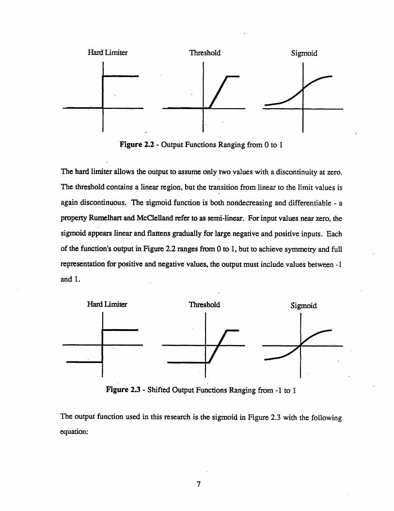
The hard limiter allows the output to assume only two values with a discontinuity at zero.

The threshold contains a linear region, but the transition from linear to the limit values is

again discontinuous. The sigmoid function is both nondecreasing and differentiable - a

property Rumelhart and McClelland refer to as semi-linear. For input values near zero, the

sigmoid appears linear and flattens gradually for large negative and positive inputs. Each

of the function's output in Figure 2.2 ranges from 0 to 1, but to achieve symmetry and full

representation for positive and negative values, the output must include values between -1

and 1.

Hard Limiter Threshold Sigmoid

/1LZFigure 2.3 - Shifted Output Functions Ranging from -1 to 1

The output function used in this research is the sigmoid in Figure 2.3 with the following

equation:

7

Threshold Sigrnoid

f(x, ) = 2 -0.51 -Ax

where x is the input to the sigmoid and X is a constant determining the steepness of the

slope at the origin.

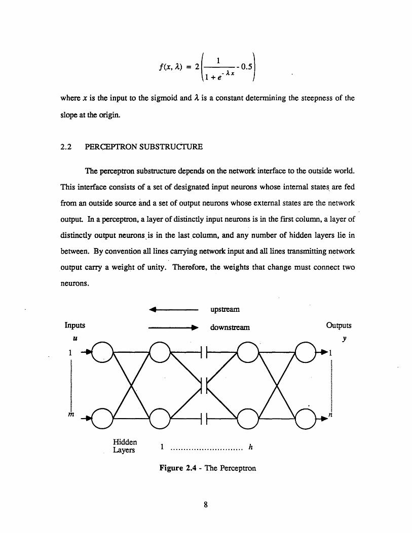
2.2 PERCEPTRON SUBSTRUCTURE

The perceptron substructure depends on the network interface to the outside world.

This interface consists of a set of designated input neurons whose internal states are fed

from an outside source and a set of output neurons whose external states are the network

output. In a perceptron, a layer of distinctly input neurons is in the first column, a layer of

distinctly output neurons, is in the last column, and any number of hidden layers lie in

between. By convention all lines carrying network input and all lines transmitting network

output carry a weight of unity. Therefore, the weights that change must connect two

neurons.

.4

Inputs

u

upstream

downstream Outputs

Y

n

HiddenLayers 1 ............................ hLayers

Figure 2.4 - The Perceptron

8

1

m

The perceptron in Figure 2.4 contains m inputs, n outputs, p neurons, and h layers.

The network input vector u and the output vectory are defined as:

I / I U. I

' IlU2

U I

'°"'I

I V I

Y2

A.Yn

The vectors of the neuron internal state net and external state o are defined as:

net =

nert

net2

0 =

I - I

r01

02

The output vector y is a subset of the output vector for all neurons, o.

2.3 THE PERCEPTRON AS A CONTROLLER

The perceptron as a compensator in a control loop establishes a mapping between

its input and output neurons. The input neurons receive the measured state variables of the

plant and the output neurons transmit the control variables to the plant. A simple problem

9

11

I

V

. a.

I "'

0 1

| .

with two inputs and one output can be visualized in two-dimensions as a phase plot. The

range of the two input values are graphed along the x and y axis. For any state of the plant

there exists a value on the graph for the output.

u = f(x,y)

Though the visualization of the decision region is difficult, this argument can be generalized

to any number of m inputs and n outputs.

The power of a perceptron to solve a particular mapping from input to output

increases with the addition of hidden layers. Furthermore, the flexibility of a perceptron

depends on the complexity of the decision shape it can create in a mapping space. A simple

example attempts to separate the two classes A and B in a two-dimensional mapping space.

A perceptron with no hidden layer can only separate the classes by a hyperplane (or line in

two dimensions). A perceptron with one hidden layer effectively separates the classes

using open or closed convex regions, whereas a perceptron with two or more hidden layers

can form an arbitrary boundary.

No Hidden One Hidden Two HiddenLayer Layer Layers

Figure 2.5 - Possible Decision Regions for Various Perceptron Structures

Since the number of hidden layers defines the input/output capabilities of the

network, the complexity of the desired controller dictates the network structure. If the

10

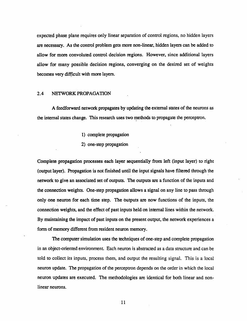
expected phase plane requires only linear separation of control regions, no hidden layers

are necessary. As the control problem gets more non-linear, hidden layers can be added to

allow for more convoluted control decision regions. However, since additional layers

allow for many possible decision regions, converging on the desired set of weights

becomes very difficult with more layers.

2.4 NETWORK PROPAGATION

A feedforward network propagates by updating the external states of the neurons as

the internal states change. This research uses two methods to propagate the perceptron.

1) complete propagation

2) one-step propagation

Complete propagation processes each layer sequentially from left (input layer) to right

(output layer). Propagation is not finished until the input signals have filtered through the

network to give an associated set of outputs. The outputs are a function of the inputs and

the connection weights. One-step propagation allows a signal on any line to pass through

only one neuron for each time step. The outputs are now functions of the inputs, the

connection weights, and the effect of past inputs held on internal lines within the network.

By maintaining the impact of past inputs on the present output, the network experiences a

form of memory different from resident neuron memory.

The computer simulation uses the techniques of one-step and complete propagation

in an object-oriented environment. Each neuron is abstracted as a data structure and can.be

told to collect its inputs, process them, and output the resulting signal. This is a local

neuron update. The propagation of the perceptron depends on the order in which the local

neuron updates are executed. The methodologies are identical for both linear and non-

linear neurons.

11

2.4.1 Complete Propagation

To achieve a complete propagation the neurons must be updated beginning with the

input layer. The methodology continues updating the neurons by progressing through the

network layers to the output layer. This has the effect of carrying the network input

downstream from the input layer to the output layer. The output of the last neuron reaches

steady-state given a constant input.

1 * 2 ' 3 * 4

Figure 2.6 - Complete Propagation Sequence

2.4.2 One-Step Propagation

One-step propagation begins on the output layer and works upstream to the input

layer. In this fashion, each neuron fires using old external states of neurons yet to update.

This technique does not require storing of old values to achieve memory in the system.

4 - 3 4 2 4 1

Figure 2.7 - One-Step Propagation Sequence

2.5 TEACHING

Teaching a network means changing the neuron connection weights. Not all neural

12

networks are taught, some begin with a defined set of weights which never change. The

basic learning rule for a perceptron proposed by Hebb increases the weights along the paths

whose signals tended to produce the desired output. A weight along a path whose signal

caused the output to diverge from the desired could be decreased or kept unchanged.

Hebbian learning is rarely used in this simple form today, but almost all teaching

algorithms are descended from this manner of adjusting the connection strength.

This research teaches the perceptron using a group of learning rules known as error

propagators. Each of these algorithms involve a number of steps.

1) Evaluate the performance of the network

2) Generate a local error at the point of evaluation

3) Propagate the local error to all contributing neurons

4) Change the weights between neurons according to their error

Error propagators employ a gradient descent in the local error with respect to weight

changes.

Rumelhart and McClelland's learning rule, called backpropagation, evaluates the

network performance using desired input/output pairs. The local error originates at the

network output. These errors are then recursively "backward propagated" to all the

contributing neurons. The connection weight between two neurons changes according to

the error of both neurons. When the network operates as a compensator in a control loop,

backpropagation requires knowledge of the network output or control action given an input

or state of the plant. This constrains the weights to converge on a preset control law.

This research proposes a new algorithm, calledforpropagation, which generates a

local error based on a comparison of the actual and target network input. This evaluation

uses a desired plant state or network input instead of a desired control action to the plant.

The local error originates at the inputs and is "forward propagated" to the output neurons

13

using a term which relates the change in input to an associated change in output.

Forpropagation then proceeds like backpropagation using the neuron errors to adjust the

weights. The weights then converge on values that result in a target response of the plant

regardless of the necessary control action.

14

3 NETWORK TEACHING STRATEGIES

This chapter compares two methods for teaching neural networks which operate as

compensators in a control loop. Both algorithms, classified as error propagators, use

gradient descent techniques to adjust the connection weights of a perceptron with semi-

linear neurons. Backpropagation is a popular method effective in many problems, but not

well-suited for control applications. Since backpropagation requires input/output pairs, the

network output must be known which requires prior knowledge of the desired

compensator. This constrains the network to converge on a predetermined set of weights.

As a result, a new technique termed forpropagation specifically addresses the problem of

teaching a compensator. Section 3.1 discusses the architecture of a controller with a

network compensator. Section 3.2 introduces issues related to the general method of error

propagation teaching algorithms. Sections 3.3 and 3.4 give quick overviews of the

backpropagation and forpropagation algorithms.

3.1 THE NEURAL NETWORK AS A CONTROLLER

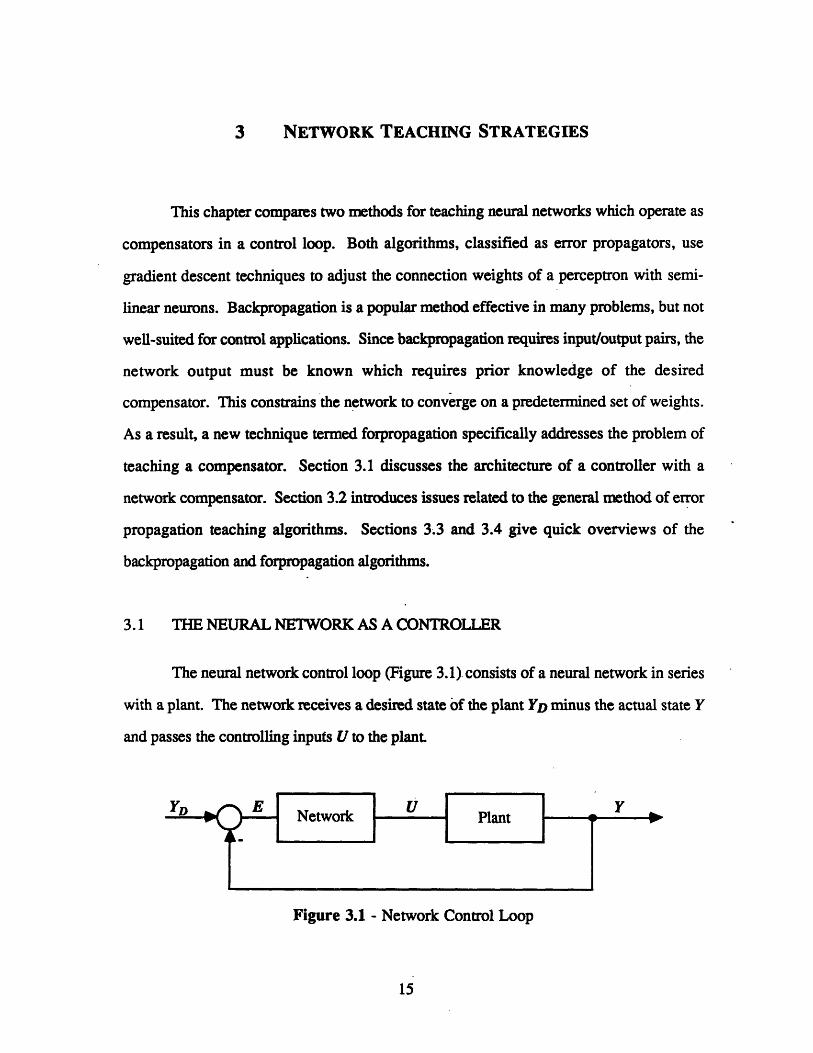
The neural network control loop (Figure 3.1) consists of a neural network in series

with a plant. The network receives a desired state of the plant YD minus the actual state Y

and passes the controlling inputs U to the plant.

Figure 3.1 - Network Control Loop

15

The network acts as a compensator in the control loop. By changing the connection

weights the network can produce any desirable transfer between input and output. If the

network maintains memory either from resident neuron memory or through one-step

propagation, then it is a dynamic compensator. A network continually taught while

operating within the control loop is an adaptive compensator.

The connection weights change according to a learning rule which uses an

evaluation of the network's performance as a controller. One current approach to this

problem uses the backpropagation algorithm which evaluates the network output based on a

desired input/output pair. Unfortunately, this requires complete knowledge of the desired

control function. At best, the network will learn a target controller but cannot adjust the

compensator parameters on-line.

The main theoretical contribution of this research is a second approach to teaching a

network in a control loop. This new approach, named forpropagation, produces an

evaluation at the network input based on the difference between the actual state variables

and their commanded values. By tracking the plant state exclusively there is no need to

specify an initial controller, the network converges on the weights necessary to control the

plant. If the dynamics vary over time, the network senses the error and adjusts the weights

accordingly.

3.2 TEACHING NEURAL NETWORKS USING ERROR PROPAGATION

The method for teaching networks using error propagation produces a gradient

descent in error with respect to weight changes. At every step, the routine calculates theaE

partial derivatives F of the total error with respect to each weight then moves a certainaE

distance in the direction of the negative gradient vector W. Assuming no problems

with local minima, the error will ultimately reach zero. The following sections introduce

topics common to all error propagation methods.

16

3.2.1 The Lesson

Error propagation of all types adheres to a strategy of data presentation with weight

changes known as the lesson structure. Sometimes the teaching session occurs off-line in a

procedure calledfixed learning. After the network is taught, it is used in an application

with fixed weights. Another common method involves on-line or adaptive learning. Here

the weights are continuously adjusted while the network performs its function.

3.2.2 Learning Rate and Momentum

The learning coefficient T7 dictates how quickly the weights change. Ideally this is

as high as possible without leading to oscillations or instability in the weight changes. An

effective way to increase the learning rate while filtering out high frequency oscillations is

to include a momentum coefficient I which includes the effect of the last weight change on

the current change. This keeps the weights from adjusting drastically due to high-

frequency noise. Some researchers set i + T7 = 1, while others let the coefficients vary

freely. A typical setting would be 4u = 0.9 and = 0.1.

3.2.3 Periodic Updating

Often it is desirable to accumulate the weight change over several presentations of

data and then incrementally adjust the weights. Sejnowski [27, 28] used this procedure

when he presented the letters of a word sequentially and then adjusted the weights once for

each word according to the summed contribution of each letter. This method allows the

network to treat a sequential set of data as one.

3.2.4 Weight Initialization

Weight initialization with most teaching rules is a crucial step incorporating prior

information. With error propagation the network can start as a clean slate. However, it is

17

necessary to initialize the weights to small random values to break the symmetry of the

network and allow connections to assume different weights. Usually the weights are

uniformly distributed over a small range of positive and negative numbers.

The closer the initial weights are to the desired final answer, the faster the network

converges. In addition, if the starting weights are much larger than the target values, the

network receives misleading information from the plant resulting in weight instability.

Assuming the neurons operate in their linear region, the network weights could be

initialized using the best information of the final control law. This represents a "first-cut

linear guess" at the desired compensator.

3.3 BACKPROPAGATION

Backpropagation in feedforward networks employs the generalized delta rule to

teach a network input/output pairs. The method adjusts the connection weights by

evaluating the error of the output layer. A teaching session using backpropagation cycles

through a number of input/output pairs. For each presentation, the weights change slightly

to register the effect of that pair on the final network.

After a sufficient teaching period, the network possesses the ability to associate an

input with a corresponding output. For example, suppose the network is taught using

desired outputs that are the squares of the corresponding inputs. Also assume only the

pairs of odd numbers and their squares are used to teach the network. In theory, after the

teaching is complete, the network will not only output the squares of the odd number

inputs, but it should also build the association to estimate the even number squares.

3.3.1 Teaching Controllers Using Backpropagation

Figure 3.2 shows the network control loop augmented by a backpropagation

adapter. Since the network adjusts the weights while attempting to control the plant this is

18

a form of adaptive learning. The reference in the figure represents the desired compensator

for the plant. The network at best can only mimic the reference. structure. If the reference

compensator is poorly designed or the plant dynamics are not well known, the network

controller cannot perform well. The adapter receives the residual R and applies the rules of

backpropagation to the network.

Figure 3.2 - Backpropagation Control Loop

This design builds a compensator into the associative memory of the network.

When the network operates as a controller, it associates certain states of the plant with

approximate control actions. Unfortunately, the approach requires knowledge of a

controller and assumes no plant modelling errors. In most control systems, the desired

state of the plant is known but not the desired control action. This need for a desired output

severely limits the capabilities of backpropagation as a teacher for a controller.

3.3.2 Applying Backpropagation

Teaching a network using backpropagation, or any other neural network teaching

algorithm, requires adherence to a number of rules. Foremost, the network must be a

perceptron with semi-linear neurons. Special attention must be paid to the ordering of steps

19

to change the weights as well as the setting of a number of teaching parameters.

Backpropagation is applied in two steps. First, the routine generates the neuron

errors recursively starting at the output using the following equations for output and hidden

neurons:

output neurons j = (tj -o) f'(net)

hidden neurons 6, = f(netj) X wjkk

where t is the target output and oj is the actual output. Second, the weights are changed

according to:

Awij ( + 1) = Tl 6i oi + p Awij(P)

where il is the learning coefficient, # the momentum coefficient, Awi (P) is the weight

change made during the previous lesson, and Awij ( + 1) is the weight change for the

current lesson.

3.4 FORPROPAGATION

Forpropagation adjusts the connection weights based on an evaluation of the inputs.

The weights continually adjust as the network attempts to control the plant. If the error

grows too large or the plant becomes unstable, the system reinitializes and a new lesson

begins. After a number of lessons, the weights converge on values that produce a desired

response in the plant. Forpropagation is a natural methodology allowing the user to specify

a performance for the plant. If the plant dynamics change, the network senses the error and

adjusts the weights to again achieve the desired response.

3.4.1 Teaching Controllers Using Forpropagation

Figure 3.3 shows the network control loop now augmented by a forpropagation

20

adapter. The reference in the figure represents the overall desired plant response. The

adapter receives a residual based on the desired and actual plant states and applies the rules

of forpropagation to the network.

r

Figure 3.3 - Forpropagation Control Loop

Each of the major components of Figure 3.3 are discussed at length in the upcoming

chapters.

3.4.2 Applying Forpropagation

Forpropagation, like backpropagation, requires a perceptron with semi-linear

neurons. Issues related to gradient descent techniques also remain unchanged. A complete

derivation of the forpropagation algorithm explaining all terms and notation appears in

Chapter 7.

Forpropagation performs three operations. First, it calculates the propagation terms

beginning at the output using the two equations for the output and hidden neurons:

output neurons

hidden neurons

Pkk = f'(netk)

Pik = f(net,) E w ijPjkJ

21

Second, the routine generates the neuron errors 6 for both the hidden and output neurons

using the residual vector R.

(h)output neurons a8k = -R h kP k k

(h) outputshidden neurons 6 = -R h hpjk

k

where rhkis defined as the dynamic sign term. A neuron error represents how

forpropagation changes the neuron's weighted sum input (i.e. - its upstream connection

weights) to decrease the value of the residual. Finally, the weights are adjusted using the

equation:

residuals (h)

Awij(p+ l) = oi 6 + Awij(P)h

where 77 is the learning coefficient, p the momentum coefficient, Awij (p) is the weight

change made during the previous lesson, and Awj (p + 1) is the weight change for the

current lesson.

22

4 THE PLANT

The dynamic problem chosen for the neural network controller is the inverted

pendulum on a cart. This chapter defines the plant and its state variables and presents the

derivation of the equations of motion.

4.1 PROBLEM DEFINITION

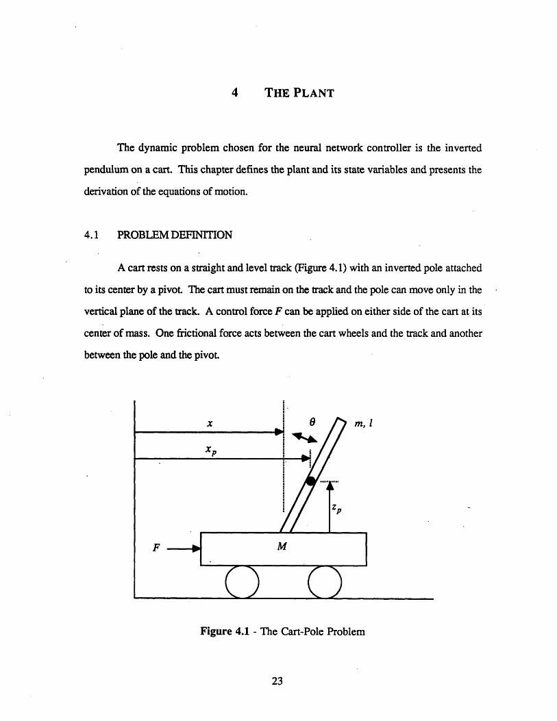
A cart rests on a straight and level track (Figure 4.1) with an inverted pole attached

to its center by a pivot. The cart must remain on the track and the pole can move only in the

vertical plane of the track. A control force F can be applied on either side of the cart at its

center of mass. One frictional force acts between the cart wheels and the track and another

between the pole and the pivot.

Figure 4.1 - The Cart-Pole Problem

23

Full-state feedback includes the cart's position X and velocity X and the pole's angular

position 0 and velocity . The two measurements Xp and Zp are used in the Lagrangian

derivation of the equations of motion. The important parameters include:

g = gravity (9.8 m/sec2 )

M = mass of cart

m = mass of pole

L = half length of pole

p = coefficient of friction of cart on track

/Up = coefficient of friction of pole on cart

4.2 EQUATIONS OF MOTION

To derive the equations of motion of the cart-pole problem using Lagrangians, first

define the coordinate transformations Xp and Zp, and their first derivative:

Xp = X+Lsin8

Xp = X + LcosO 0

Zp = L cosO

Zp = - L sine

Now write the kinetic energy of the system Ek including terms for the cart's translational

energy and the pole's translational and rotational-energy.

Ek = MX +m + + --m L 0

Substituting the definitions of Xp and Zp and simplifying:

24

.2 .21 '2 m L2 +mLcosX

Ek = (M+m)X +mL

The potential energy of the system Ep depends only on the pole.

Ep = mgZp = mgLcosO

Now write the Lagrangian of the system.

1 .2 2.2 A = Ek -E p = (M+m)X +-mL 9 +mLcosOXO-mgLcos9

The forcing terms for X and 0 are:

xx = F-c I sgn(X)

The = -balance equations in both Xand are defined as:The force balance equations in both X and O are defined as:

d aAd.t'a

d ad

aA

ax

aA- =

Evaluating the above equations and rearranging gives the two equations in X

describe the motion of the cart-pole.

F(t) + m L (t) sin(t) - (t) cos(t) -F(t) + m L 9 (t) sin (t) - 0t) coso(t)-)X(t) M+m

gsine(t) + cosO(t) -a.. _

.2F(t) - m L 9 (t) sinO(t)

M+m+csgn(X(t))

M+m

These are the two equations used in the cart-pole simulation. For a given state of the plant,

25

and 0 that

t =

Pp 9(t)

mL

PC sg~t))

the routine first determines 8 and X and then uses a numerical integration scheme to

determine the pole and cart positions and velocities. A simplified set of dynamic equations

assume:

* no friction (uc = 0 and pp = O)

* small angles (sin = 8 and cos = 1)

* cart mass is much greater than pole mass (M + m = M and m = 0)

Now the equations defining the motion of the cart-pole are:

* g F= go .FL L'M

FX=-MM

where L' is the effective pole length defined as:

1 L2 2L' ML2 -ML +ML2 4

= ML ML 3

These simplified state equations are used in Chapter 6 to motivate an architecture for the

neural network compensator.

26

5 THE REFERENCE

The plant and the reference controller run simultaneously and are given identical

commanded positions. The reference is a simplified plant model (no friction, nominal

dynamic parameters) with a linear control law that responds in a desired manner to control

commands. The teaching algorithm adjusts the network weights "on the fly" according to

the difference between the reference and plant states. If the deviations between the two

responses becomes significant, the system is reset and a new lesson begins. After the

teaching is completed, the network weights should converge on values that result in similar

performance of the reference and plant.

5.1 NEED FOR THE REFERENCE

The reference is necessary due to the formulation of the forpropagation algorithm.

The equations adjust the weights to achieve a gradient descent of some measure. If that

measure is the system error E, the weights constantly change to decrease E. This results in

unbounded weights since a newly commanded position of the cart is perceived as a

discontinuous increase in E. With each teaching pass, forpropagation changes the weights

to move the cart faster and faster to the commanded value. Eventually the gains of the

network compensator become too large and the system reaches instability.

As an alternative approach, forpropagation uses the residual R which is the

difference between the actual plant state and the desired reference state. The reference and

the plant receive identical commanded positions and the reference "shows" the plant the

appropriate response. Here forpropagation is well-suited to null the residual by adjusting

the connection weights. If the cart is moving too fast with respect to the reference, the

weights change to slow the cart down; and, if the cart lags the reference, the weights

27

change to speed up the response. The reference always provides the identical response

characteristics for the plant to follow. If significant changes are made to the plant

dynamics, the weights will again adjust to mimic the reference.

5.2 BACKGROUND ON MODEL REFERENCE

This section discusses a number of issues related to teaching with a reference.

Most of the observations result from experimental work with the neural network controller

simulation.

5.2.1 Initial Information

Ideally, the initial values of the network weights are as close as possible to the final

weights after convergence. In this situation, the controller slightly adjusts its internal

representation to satisfy the performance requirements. However, if the initial network

weights are significantly different from the target, the controller must go through an

intensive and carefully structured learning session.

5.2.2 System Reset

System reset is a necessary action when teaching the network in a "carefully

structured learning session." As the deviations between the plant and reference increases,

the chance for spurious weight change and instability also increases. Consider the simple

-example when the cart-pole begins at X = 0 and is commanded to a positive position P.

Assume the plant lags behind and the reference reaches P first. The reference then

overshoots the commanded position and begins moving back to P with a negative X and

a negative 9c. Meanwhile the plant has yet to reach P and continues with a positive X

and a positive Oc. At that instant the network controller receives ill-advised information on

28

the desired pole position and desired cart velocity. In this situation the system should be

reset.

-4-

commandedposition

P

Figure 5.1 - The Lag Problem

The system also maintains a reset limit on the absolute pole position and velocity to insure

no teaching past the "point of no return". Here the maximum control force F cannot

recover a falling pole. This issue of resetting the system for another lesson is critical and

should be addressed with much care.

5.2.3 State Variables to Track

Tracking a state variable means comparing its value with the reference over time and

generating an error used in adjusting the weights. In the cart-pole problem there are four

possible state variables to track: pole position, pole velocity, cart position, and cart

velocity.

Tracking Only Cart Position and Velocity

The final objective is to control the cart position so it seems logical to choose to

track only the cart position and its velocity. The only requirement on the pole is that it

29

remains erect regardless of the time history of its position and velocity. Furthermore, with

a change in cart mass or pole length, the network controller will undoubtedly require a

different response in the pole to achieve the same response in cart position. This may

present a problem when the network controller commands an unrealistic and irrecoverable

pole position. However, the thresholding effects of the neurons do limit this action.

Tracking All State Variables

This approach is not recommended unless problems arise with keeping the pole

upright. Perhaps an acceptable approach would be to leniently track the pole position and

velocity to insure balancing.

5.2.4 Weight Update Interval

The weight update interval is a crucial setting in the learning algorithm. One

approach updates the weights much faster than the system's highest natural frequency.

This offers quick learning and recovery, but is very sensitive to higher order disturbances

and noise which often lead to instability. Another approach allows the network controller

to perform for a long interval of time without changing the weights. This "mimic and

adjust" procedure produces a more stable system impervious to higher order effects, but

relies on many lessons to teach the desired weights.

5.2.5 Weight Update Test

The simulation uses two modes of update. The mandatory or forced update always

adjusts the weights at the scheduled time regardless of the performance of the network

controller. This approach continuously adjusts the weights even when the plant closely

follows the reference. The second method, the optional update, changes the weights only

if the adapter error is above a certain threshold.

30

5.3 DESIGN OF THE REFERENCE

The reference controller design assumes nominal dynamic parameters - a cart mass

M of 1 kilogram and a pole length L of 1 meter. The controller commands F in the range of

±10 Newtons and limits 0 c to ±15 degrees. The controller was designed using pole

placement to achieve the quickest possible response in X with a of approximately 0.7.

F = 69.3 0+ 13.2 + 4.9X+2.0(X- X )

The reference response, used by the forpropagation algorithm, first reaches an Xc of 5 m in

5.44 sec, overshoots by 4.4%, and settles to within 2% in 9.56 sec.

2

Err0r

0

(m)

-2

-4

-6(sec)

0 5 10 15

Graph 5.1 - The Reference Response

The task of this controller is to produce a reference response used in the

forpropagation algorithm. The controller operates on an unchanged plant model of M = 1

kg and L = 1 m, producing the identical reference response for all of the experiments. As

the plant dynamic parameters change, the network controller attempts to mimic this

response from the reference. Plant perturbations in pole length or cart mass that take place

31

in the control loop are not reflected in the reference model, thus the reference response

always remains the same.

32

6 THE NETWORK

This chapter introduces the operation of the neural network as a fixed-gain

compensator for the plant in a feedback loop. The network topology is specific to the

control problem. In this research, the number of input neurons and output neurons match

the number of state variables and control variables, respectively. Furthermore, with the

cart-pole problem, the network infrastructure resembles the inner and outer loop

organization of the classical compensator.

6.1 THE NETWORK CONTROL LOOP

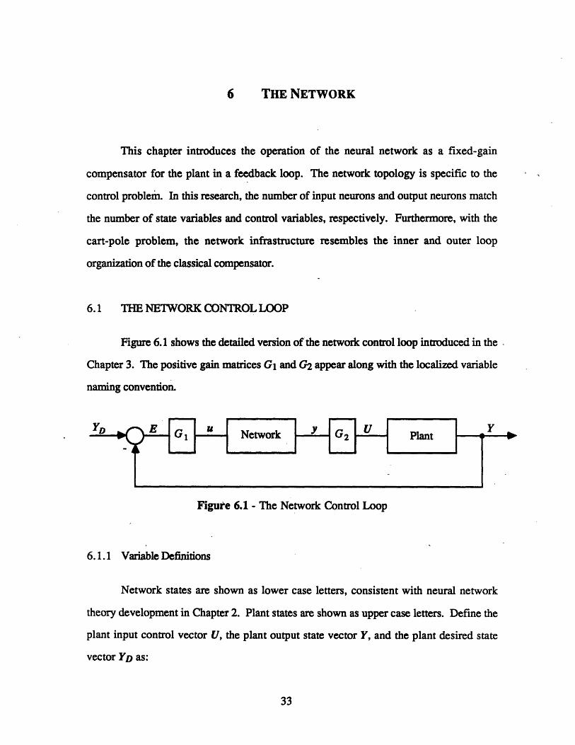
Figure 6.1 shows the detailed version of the network control loop introduced in the

Chapter 3. The positive gain matrices G1 and G2 appear along with the localized variable

naming convention.

Figure 6.1 - The Network Control Loop

6.1.1 Variable Definitions

Network states are shown as lower case letters, consistent with neural network

theory development in Chapter 2. Plant states are shown as upper case letters. Define the

plant input control vector U, the plant output state vector Y, and the plant desired state

vector YD as:

33

I FTT aI1

U2

Uj

ti1

Y2

Z D1

YD2

vOF

The network receives the system error E equal to the desired state YD minus the actual

state Y and passes the controlling inputs U to the plant. The output y of the network is a

function of the input u, the connection weights, and sometimes the old output states.

6.1.2 The Neural Network

The network box contains the network structure, interconnection weights, and

propagation function for the perceptron. Complete propagation allows the network to settle

to a steady state for each time step. The network output is a function of only the current

inputs and the weights. One-step propagation passes a signal one layer forward for each

time step. The output for this type of propagation is a function of the current input, the

network weights, and the effects of previous input values held on signal lines within the

network. This propagation incorporates memory and is used later in a design of a

partial-state feedback controller. Techniques for complete or one-step propagation of linear

or non-linear perceptrons appear in Chapter 2.

6.1.3 The Plant

The plant contains the control problem dynamics. It receives a control action and

outputs its state variables. A full-state feedback controller uses all independent state

34

a Y . I

I �· -- m ·

U= Y

I �I

9 TZ S as a

V _ ·2

YD=

I - I m r

variables to control the plant whereas a partial-state feedback controller uses only a subset.

The experimental work of this paper uses an inverted pole on a cart as the plant (see

Chapter 4).

6.1.4 The Gain Matrices

The gain matrices G1 and G2 contain positive, non-zero entries along the diagonal.

They are used to appropriately scale the variables of the plant and network. The gains in

G1 are chosen to keep the network input bounded by the sigmoid function. A gain on a

state variable causes the sigmoid to saturate at a particular value for that variable. This

saturation point depends on the desired operation envelope of the plant. The experiments

of Chapter 9 used the following four gains in G1 for the state variables of the cart-pole.

The gains in G2 determine the relationship between the network outputs and the controlling

inputs to the plant. For the cart-pole problem the single network output is multiplied by a

factor of 10 to produce a control force range of ± 10 Newtons.

6.2 OPERATION OF THE NETWORK CONTROL LOOP

At each time step, the simulation integrates the equations of motion of the plant and

updates the control action by propagating the network. At a less frequent rate, the program

adjusts the network interconnection weights based on the performance of the controller.

Nominally, the equations of motion and control action are updated at 25 Hz while the

weights are adjusted at 5 Hz. After 5 time steps of normal fixed-gain operation, the

35

Gains in G1

0 8.0

o 4.0

X 0.3

X 0.9

network weights are adjusted. Discussion of the weight change algorithm appears in the

Chapter 7.

There are three ordered events for one complete time step of the network control

loop. First, the system determines the error vector:

E =YD-Y

Next, it propagates the network, either complete or one-step, using the input vector:

u = G1E

The full-state controllers use complete propagation which allows the network to' settle to a

steady-state output. Partial-state controllers require a memory of past input values and use

one-step propagation. Finally, the system numerically integrates the plant dynamics using

the new controlling input vector

U = G2y

6.3 CONTROLLER ARCHITECTURES

This section establishes the infrastructure of the network used as a full-state

compensator for the cart-pole problem. Since all necessary state variables are available to

control the plant, the compensator requires no memory and uses complete propagation.

Steps are taken to develop controllers using classical methods which in turn motivate the

design of analogous network structures. Section 6.3.1 derives a classical controller to

balance the pole and proposes a network counterpart. Section 6.3.2 develops a

compensator to control the cart position while balancing the pole and again presents an

analogous network structure. Since the purpose of this section is to determine the general

structure of the network compensator, a simple model of the cart-pole will suffice.

36

6.3.1 The Full-State Pole Position Controller

The initial task of the cart-pole problem is to balance the pole, or ideally, control the

pole position. First, the problem is solved using classical control techniques and then an

analogous design of a network is proposed.

Classical Control Technique

Using the simplified state equations of the cart-pole found in Chapter 4, the

expression governing 0 including the forcing term F is:

O- + L'M =0

where g is the force of gravity, L' is the effective length of the pole, and M is the mass of

the cart. Rearrange and differentiate to get the transfer function in terms of the Laplace

operator s.

· S

0 L'M

The resulting control loop is:

Figure 6.2 - Theta Control Loop

37

A judicious choice of K3 and K4 places the two closed loop poles in any desired

configuration. From the block diagram in Figure 6.2, assuming Oc is zero, F can be

rewritten as:

F = -K 3K4 + K40

Combine the above equation with the simplified state equation and factor out 0.

0 +L'M + L'M 0[s2 + VMS ( | + t~i~f,4)] = 0

Compare this result to the general second order equation:

2 2s + 2 oO)no + )O 0

where Co is the damping coefficient and o0 is the natural frequency. The two equations

determining K3 and K4 for a given choice of 'o and ono are:

2

Con + L'K3 =

2 Co hO

K4 = 2 0nwoL' M

The preceding derivation of the O controller using classical techniques does not constrain

the control input F. First choose a desired eo (usually .707) and then in an iterative

procedure choose the desired aon and check if the resulting gains give a reasonable control

action. To realize a large cono requires a large control input F. After readjustment of cOno to

fit within the control limits of the system, the final transfer function is:

2

0 Csteno + Lo

O 2 2s + 2 oOwns + OnO

38

Analogous Network Controller

The equivalent neural network controller requires two gains on the angular position

and velocity. The final network structure for the 0 controller is simple requiring only two

input neurons and one output neuron.

6

6

F

Figure 6.3 - Network Structure of Theta Controller

Assuming Oc is zero and the neurons operate in their linear region, the corresponding

control law as a function of the perceptron weights is:

F = w23 9 + W13(0- e )

6.3.2 The Full-State Cart Position Controller

The next task is to integrate the results of the 0 controller into a complete design to

control the cart's position while balancing the pole. Again the method involves the classical

approach leading to an equivalent network structure.

39

Classical Control Technique

The design of the control loop for X requires an important assumption. If the

natural frequency of the loop is sufficiently larger than the natural frequency of the X

loop, then there are two approximations. First, the transfer from Oc to 0 in the X loop is

unity. With respect to the slow X loop, the loop maintains virtually no error. Secondly,

the design of the X loop controller ignores the second order term in 0.

g" @+L' = °

This equation, using the first assumption, becomes:

X g = g Oc

The block diagram for the X loop is now second order and can be written as:

Figure 6.4 - Simplified X Control Loop

This problem with the important assumptions is identical to. the loop design but with a

simpler plant. Wise choices of K1 and K2 will place the two closed loop poles in any

desired configuration. With Xc treated as zero, the equation governing X is now a function

of Oc

X =g O = -K 1K 2 gX - K 2 gX

Rearrange and factor out X:

40

X[s2 + K2gs + KIK 2g]= 0

Again compare this equation to the standard second order system to find the equations for

K1 and K2 given a ax and w,n.

0)nxK1 =2 x

2 x nxK2

The X control law does not explicitly limit the internally commanded 0. Again,

choose an aox and determine if it is attainable. A large AOnx in the X loop requires a large

Oc which the controller may not be able to handle. It is important to define reasonable

operating regions for the controller or include a limiter in the loop.

After choosing the two gains for the inner loop 0 controller and the two gains for

the outer loop X controller, the final control law is:

F = K4 0 - KK - K2K3K4 - K 1K2 K3 K4(X- X)

also in block diagram form:

Figure 6.5 - Full X Control Loop

and as a transfer function:

41

A

X

Xc

2 2

S + 2 nO s + -OnS -+ 2 nxInO + L| nxonO L+ 2Creones + OneL' S L

Analogous Network Controller

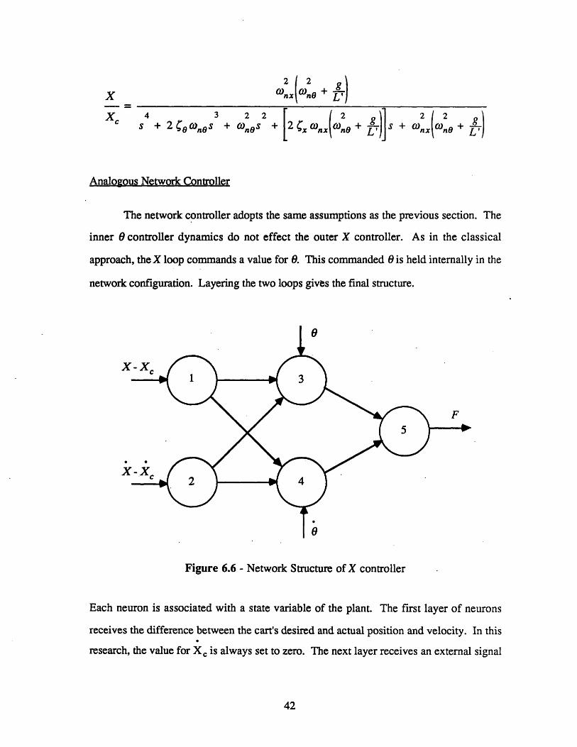
The network controller adopts the same assumptions as the previous section. The

inner controller dynamics do not effect the outer X controller. As in the classical

approach, the X loop commands a value for 9. This commanded 9 is held internally in the

network configuration. Layering the two loops gives the final structure.

0

X

X

F

a

Figure 6.6 - Network Structure of X controller

Each neuron is associated with a state variable of the plant. The first layer of neurons

receives the difference between the cart's desired and actual position and velocity. In this

research, the value for Xc is always set to zero. The next layer receives an external signal

42

of the actual angular position and velocity of the pole. The network internally generates the

negative of the desired signals for pole position and velocity and feeds these values into the

second layer of neurons. As a result, nodes 3 and 4 receive the difference between the

desired and actual pole position and velocity. The control law as a function of the network

weights with the neurons operating in the linear region is:

F = (w 3 5 w13+ W4 5 W14) (X-X)

+ (w 35 w2 3 + W4 5 W24) X + w3 5 0 + w 45 0

Since there are six weights to determine four control gains, there is not a unique solution of

weights for a particular control law.

43

7 THE ADAPTER

The adapter implements the forpropagation algorithm to adjust the network weights

according to a measure of error. This error or residual is the difference between the

measured state variables of the plant and their corresponding desired values. Section 7.1

presents the architecture of the forpropagation control loop. Section 7.2 introduces a

summary of the operation of the adapter with emphasis on the three steps necessary to

apply forpropagation. Finally, Section 7.3 shows that the forpropagation -weight change

algorithm performs a gradient descent.

7.1 THE FORPROPAGATION CONTROL LOOP

The forpropagation control loop appears in Figure 7.1. The network input u and

output y are lower case whereas the plant input U and output Y are upper case. G1 and

G2, discussed in Section 6.1.4, are the gain matrices that scale the variables of the plant

and network.

Figure 7.1 - Forpropagation Control Loop

44

The model reference receives the commanded state of the plant YD and outputs the

desired plant response YM. The adapter uses R, the difference between the actual plant

output Y and YM, to adjust the network weights. This residual R has the same dimensions

as the network input u.

I y, - ,.. \ /R, \

R =

Rj 2

D.

m- Mm/ \ m

The adaptive error e is a scalar and is defined as:

e=-R R2

As e decreases, the actual plant response closely resembles the reference response. The

weights are continually updated until the adaptive error e is below a particular threshold.

7.2 OPERATION OF THE ADAPTER

The adapter changes the individual neuron connection weights while the network

operates as a compensator in the control loop. The adapter receives the residual R,

calculates the adapter error e, and determines whether the weights should change. If is

above a preset threshold, the weights are adjusted according to the forpropagation

algorithm.

Forpropagation, derived and discussed in Section 7.3, performs a gradient descent

in the adaptive error E with respect to network weight changes. A summary of the weight

adjustment algorithm proceeds in three steps. Step 1 calculates the propagation terms p

beginning at the output using the two equations for the output and hidden neurons.

45

m r -·

2 - M2

.

hidden neurons

output neurons

Step 2 generates the neuron errors a for b

residual vector R.

hidden neurons

output neurons

Pik = f'(net) X w ijPjk

Pkk = f'(netk)

oth the hidden and output neurons using the

(h) - otutsj) = -Rh L ChkPjk

k

(h)

k = -RhIghkPkk

where lrhk is defined as the dynamic sign term. Finally, Step 3 adjusts the weights using

the equation:

. residual (h)

Awij(p + l) = n oi S + aw (p@)h

where is the learning coefficient, u the momentum term, Aw (P) is the weight change

made during the previous lesson, and Awj (p + 1) is the weight change for the current

lesson.

After making the weight changes using these three steps, the newly taught network

is used in the control loop. If the adjustments do not reduce e below a preset threshold, the

process is repeated.

7.3 FORPROPAGATION ALGORITHM DERIVATION

The following is a detailed derivation of forpropagation. Many of the techniques of

gradient descent parallel the work of Rumelhart and McClelland [26]. The specific

subscript h is used in conjunction with the residual input R. Output neurons are denoted by

subscript k, while subscripts i andj refer to any neuron. The weight that connects neuron i

46

to a downstream neuron j is denoted by wij. The output of neuron i is oi and the sum of its

weighted inputs is neti.

7.3.1 Gradient Descent

A gradient descent in the adapter error e with respect to a weight change can now be

developed by showing that:

- a weight change equationawij

This relationship insures that a small change in the weight wij results in a small decrease in

the overall adapter error e. Using the chain rule, expand the left side into partial fractions.

ae ae anetj (h) anetjawu anetj aw aw i

(h)The first term 8j , defined as the error of neuron j for the residual Rh, is evaluated in

Section 7.3.2. Express the second term using the fact that the network input netj is the sum

of the upstream neuron outputs og multiplied by the connection weights wgj.

anetj a Wj

The partial derivative is nonzero for only one term in the summation, so the equation can be

simplified and evaluated.

anet a(wio) awi awij

The weight change equation -is proportional to the output oi of neuron i multiplied by the(h)

error 6j of neuronj.

aE (h)

aw =j iLi

47

7.3.2 The Neuron Error

The neuron error is defined as:() a5 e1 anetj

This expression can be expanded using partial fractions.

(h) a ase aRh

netj aR anetj

The error states how forpropagation must change the neuron's internal state, or weighted

sum input netj, to decrease the adapter error . A fieuron contributes an error term to e for

each residual Rh. To determine the error of neuron j for a particular residual Rh, sum over

all the network outputs Yk the weight change effects.

(h) aas ae outs aRh a k

i aR h k aYk anetj

This expression states that forpropagation must adjust a neuron's upstream weights in

proportion to the effect of those weights on output control commands. Evaluate the term

relating the change in e with respect to a change in a residual Rh using the definition of the

adapter error.

a(2R aR) 2+ 1 2 R)2} R2R2+ . .+jR

RhaRh aRh aRh

Now the equation can be written as:

(h) oujuts aRh ayk

-i R k ak anetj

The next two sections discuss the terms after the summation sign.

48

The Dynamic Sign

The inputs and outputs of a perceptron controller are tied to the plant. It is

necessary to know at least a crude approximation of how a network output (actuator

command) effects a residual input. The xhk term "completes the loop" and relates the

residual Rh to an output Yk. This research only uses the sign information of the

relationship between the plant input and output.

First, define xhk as the change in a residual Rh with respect to a change in the

network output Yk.

aR h

hk= ay 1,

The subscript * means "while operating about a nominal condition". This important

restriction insures that Mhk maintains the true dynamic information of the plant. In the

example of the cart-pole, if the pole falls past the "point of no return", any allowable

control force on the cart will not move the pole back to the balanced position. This instance

leads to an incorrect calculation of the 7hk term that relates the pole position to the control

force. Now assume sh. is computed when the pole is close to the vertical. Here a positive

control force F results in a decrease in and vice-versa for a negative F. This Xhk

determined about a nominal operating condition contains the correct dynamic information of

the cart-pole plant.

Rewrite the equation for lrhk using the definition of the residual Rh = Yh - YMh

and the relationship Uk = c Yk where c is a positive constant in the gain matrix G2 (see

Figure 7.1).

aRh7h =Y -ayk *

*

49

Since the model reference response YMh is unchanged by the input to the plant Uk, the

equation becomes:

arhI hk = C-

In its simplest form rk contains the sign information of the impulse response of the plant

state Yh for the controlling input to the plant Uk.

au,

During the experiments of this research, rhk does not change but could be updated

periodically using plant perturbations in real-time. Each update would represent a local

linearization of the plant controls to the state variables.

The Propagation Term

(h) aYkThe final term in the equation for the neuron error ij is anei which relates the

change in the output of neuron k due to a change in the input of an upstream neuron j.

Since the network output Yk is the external state of the output neuron k, this expression can

be generalized for any neuron i and any downstream neuron j.

aoiPi= aneti

This is the definition of the linearized sensitivity term or propagation term Pij. Essentially,

Pij represents the effects of connection weights and saturation functions along the path

between neurons i and j. A simple case will illustrate the idea. Figure 7.2 represents a

signal path from neuron 1 to neuron 3. The interconnection weights appear in the boxes.

50

netl 03

Figure 7.2 - Simple Feedforward Path

The final expression for P13 contains interconnection weights and the effects of neuron

saturation. Expand p13 using the chain rule.

ao3 aO03 anet3 a 2 anet2 aolP13 = net3= 0anet 2 1 anet

Each factor of the form:

ao- a

anet anetnet)= (net)

contributes the effect of neuron saturation which is always positive. The factor f'(netj) is

the slope of the sigmoid function at the point netj which is very small for extremely

negative or positive inputs and reaches a maximum for an input of zero (see Figure 2.3).

Each factor of the form:

anet1 a - a(wiioi)aoi = -Wgj = = ij

contributes the interconnection weight wij to the product. The final expression forpl3 is:

P13 = w 12 W 2 3 f'(netl) f'(net2) f'(net 3)

This simple exercise suggests a recursive procedure to find all of the propagation

terms for a network. First, generate the propagation term for each output neuron.

Pkk = f (nek)

Then working back from the output layer, recursively compute the propagation terms from

the hidden and input neurons to the output neurons.

Pik = f'(neti) I wijPjkJ

51

Final Expression for the Neuron Error

(h)Now the error of a hidden neuron j for the residual Rh can be written in a

simpler form

(h) outLpts

aj -= -Rh L h 7kPjk (hidden neuron)k

where rhk is the dynamic sign term between the residual h and the output neuron k, and Pjk

is the propagation term from the input of neuron j to the output of neuron k. The error for

an output neuron is simpler since it only registers the effect of its own output on the

residual h.

(h)

a k= -Rklkk (output neuron)

As an example consider a network with a single output neuron k. For each residual

h, the neuron error for both the hidden neurons and the one output neuron simplifies to:

(h)hidden 83 = -R h x hkPjk

(h)output k = -R.hhkpkk

7.3.3 Weight Change Equation

Begin with the original definition of the weight change equation.

ae ae anetjweight change equation a - -

awij anetj aW ij

Using the definitions developed in-the previous sections, sum over the weight changes for

each residual input to the network. This involves summing the errors for all the residuals h

at neuron j.

52

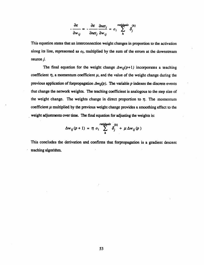
ae ae anetj residuals (h), = - 0i t 'jaw ii anetj awij h

This equation states that an interconnection weight changes in proportion to the activation

along its line, represented as oi, multiplied by the sum of the errors at the downstream

neuron j.

The final equation for the weight change Awij(p+l) incorporates a teaching

coefficient 77, a momentum coefficient g, and the value of the weight change during the

previous application of forpropagation Awiy(p). The variable p indexes the discrete events

that change the network weights. The teaching coefficient is analogous to the step size of

the weight change. The weights change in direct proportion to 77. The momentum

coefficient y multiplied by the previous weight change provides a smoothing effect to the

weight adjustments over time. The final equation for adjusting the weights is:

residuaL (h)

Aw y(p + 1) = , + PAwi (p)h

This concludes the derivation and confirms that forpropagation is a gradient descent

teaching algorithm.

53

8 IMPLEMENTATION

The Neural Network Controller Simulator, written in Common Lisp, runs on the

Symbolics 3600 computer. The program is organized into modules which perform specific

tasks. This chapter reviews the operation of the Neural-Network-Controller, Pole-Exec,

Forprop, Pole-Dynamics, and Big-Graph modules. Source listings of the Pole-Exec,

Forprop, and Pole-Dynamics programs appear in the Appendices.

8.1 NEURAL-NETWORK-CONTROLLER

This Neural-Network-Controller directs the high level control of the simulator. In

addition to organizing the graphical displays, it also contains the system menu.

Neural Network Controller

Figure 8.1 - Initial Display of the Simulator

54

Ntwork Connguretlon Neuron Informatlon Phase Plane Plot

Layered x - r - noainel type: HIDDE

Input Weightsl 360.291 01.212

C * output weights .

Interl states ".1 -.tsrnai stats: 5

-v.e -I. -. 5 5. 16 .oui lmRu: vR t thet t l.2I W.OOTh, h

Error v. Time COMMAND MENU Bart's Pole BalancerDe the tcn 9.99 .co 99.99

. Tlaeha w theted a 99.6 d a W.WMErr or V.. tis MN a 66.9O kick * oan .

Display OptbssRot Type

o..

·. I. 2.0I I

"Msurl etwork Controller connand: DynrencsNeral Ietwuok Controller connends Display Optionsnta l etwork Controller conandt

Figure 8.1 shows the display of the simulator before running an experiment called

Nominal. The window is arranged into six panes:

* Network Configuration

* Neuron Information

-* Phase-Plane Plot

* General Plot

* System Menu

* Cart-Pole

The Network Configuration pane displays the experiment name and the infrastructure of the

network. Information on the connection weights and state of the darkened neuron appears

in the adjacent Neuron Information pane. The user can click on a neuron and display the

statistics or change the neuron parameters while the simulation is running. The Phase

Plane Plot pane shows the current control decision for the cart-pole in 0 - space. The

General Plot pane displays the user's choice of single or multiple value plots of the

cart-pole state variables. The System Menu contains all of the high-level simulator

commands that allow the user to adjust on-line any of the parameters related to the

forpropagation algorithm, the cart-pole simulator, and the display. The Cart-Pole pane

displays an animated picture of the plant. The vertical line below the track indicates the

commanded position of the cart. The user can command a new desired cart position "on

the fly" by dragging the line with the mouse.

Figure 8.2 now shows a snapshot of the experiment in progress. Dark circles in

the Phase Plane Plot represent a positive control force F and light circles a negative F. The

magnitude of F is proportional to the radius of the circle. The General Plot Pane indicates

the cart position error is approaching the zero horizontal line. The Cart Pane displays

55

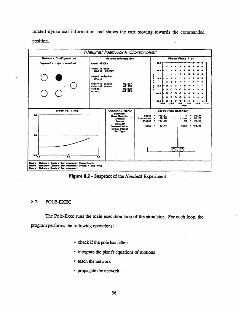
related dynamical information and shows the cart moving towards the commanded

position.

Figure 8.2 - Snapshot of the Nominal Experiment

8.2 POLE-EXEC

The Pole-Exec runs the main execution loop of the simulator. For each loop, the

program performs the following operations:

· check if the pole has fallen

· integrate the plant's equations of motions

· teach the network

· propagate the network

56

Neural Nsetwork ControllerNetwork Configuration Neuron Informatlon Phase Plane Plot

Layered x - pr - nominal type: HIDDEIN .

input ueights: * 099.147 99.229

output weights: 00 906.213 h 1. 0 0 0 e e _ C

internal state: 02.387external state: 09.983 e -. eO O0 0 o o

e nbdo: 82.98 O O O O o0 o 0

© © -3" -6.60 0 000 0 0 . a-21.0 -1S.6 -5.0 .S 15.6 21.8

Theta

Error vs. Time COMMAND MENU Bart's Pole BalancerExperiment

Phase Plane lot theta = -9.51 x = 9.94Dynamics theta-onr * 99.90 x-con - 91.20Teacher thetad = -92.15 xd = 99.56Evalutor

["'/~~~ I ~Comnd Vues tne = 03.44 kick = -09.09Dlspiay Options

Plot Type6.5

-2.5.a 2.0 4.a

I Ihural Network Controller command: ExpernimentNeural etuork Controller commend: Phase Plane PlotNeural Network Controller conmndl

. .. ~~~~~~~~~~~~~~~~~~~~~~~~~~~~~~~~~~~~~

Pole-Exec also allows the user to create, stop, start, and reset a number of user-defined

experiments.

8.3 FORPROP

Forprop contains the software to create, propagate, and teach networks. The

program builds a network given the following characteristics:

* the number and type of neurons in each layer

* the connections between each layer or neuron

* the initialization of the interconnection weights

* the type of propagation function

All experiments for this research use neurons whose internal function sums the weighted

inputs and whose output function is sigmoidal. One common sigmoid function used by

Rumelhart and McClelland ranges from 0 to 1:

f(x, ) = 1-A xl+e

but does not allow explicit representation of positive and negative values. The shifted

sigmoid function used for this research ranges- from -1 to 1:

f(x, l) = 2 1 - 0.5)

where the constant AZ determines the steepness of the sigmoid.

The neuron interconnections are directed, weighted signal lines between two

neurons. They are usually specified through simple layer-to-layer connections where each

neuron in an upstream layer feeds a signal to each neuron in a downstream layer. The code

57

also handles neuron-to-neuron and neuron-to-layer connections. Any signals of neurons

from downstream layers to neurons of upstream layers is forbidden in the perceptron

structure. The interconnection weights can be initialized over a uniform distribution range

or they can be set to specific values.

The software supports both complete and one-step propagation. A network is

propagated with external inputs fed into any of the neurons. These network inputs are

scaled to take advantage of the limiting characteristics of the neurons. The propagation

routine receives a list of values to be input into specific neurons, propagates the neurons

with. those inputs, and returns the external state of the output neurons.

The Forprop module also contains all the teacher routines necessary to adjust the

network weights using forpropagation. First, the program calculates the propagation terms

and the neuron errors given the current state of the network weights and plant. Then the

weights are adjusted using the equations derived in Chapter 7. The cart-pole simulation

runs at 25 Hz and the teacher adjusts the weights at 5 Hz, or every fifth time step. For all

experiments, the learning coefficient r7 is set to 0.01 and the momentum coefficient ]Y is set

to 0.9.

8.4 POLE-DYNAMICS

Pole-Dynamics contains all of the cart-pole simulation software. The main purpose

of this program is to update the equations for cart acceleration X and the pole acceleration

0.

X( = F(t) + m L (t) sin (t) - O(t cos (t))- csgn((t))X(t) =MM+m

58

.2

gsin6(t) +cos0(t) - F(t) - m L (t) sinO(t) + lcsgn t) p (t)

=gsine>L 4 m cos 0(t)\3 M+m )

The following simple integration filters compute the velocities and positions of the cart and

pole:

h(tl) = (t+l ) + Ath(t)

h(t+l) = (t+2.0 ) At+h(t)

Pole-Dynamics uses the same dynamic update equations to simulate the classical controller

and the model reference controller. This module also allows for uniform distribution noise

to be added to any state variable.

8.5 BIG-GRAPH

Big-Graph allows the user to plot any state variable versus time. The routine

supports dual graphs which will be used extensively in Chapter 9 to superimpose the

reference and network controller responses.

59

9 EXPERMENTAL RESULTS

This chapter compares the neural network controller to the fixed-gain classical

controller. The initial results show the network controller converges on the reference

response when the plant dynamic parameters are identical to the model reference

parameters. Furthermore, the network controller, while still being taught by the nominal

reference response, adapts quickly to significant changes in cart mass and pole length. For

the same parameter perturbations, the classical controller fails to balance the pole. Section

9.1 discusses the limitations of the classical controller while Section 9.2 presents

experiments showing the adaptability and performance of the neural network controller.

9.1 THE CLASSICAL CONTROLLER

With a commanded cart position Xc of 5 m, a cart mass M of 1 kg, and a pole

length L of 1 m, the classical controller gives the following response in cart position X.

E 0rr (m)or -2

-4

-6

60

(sec)0 5 10 15

Graph 9.1 - Classical - Response in X (M = 1 kg, L = 1 m)

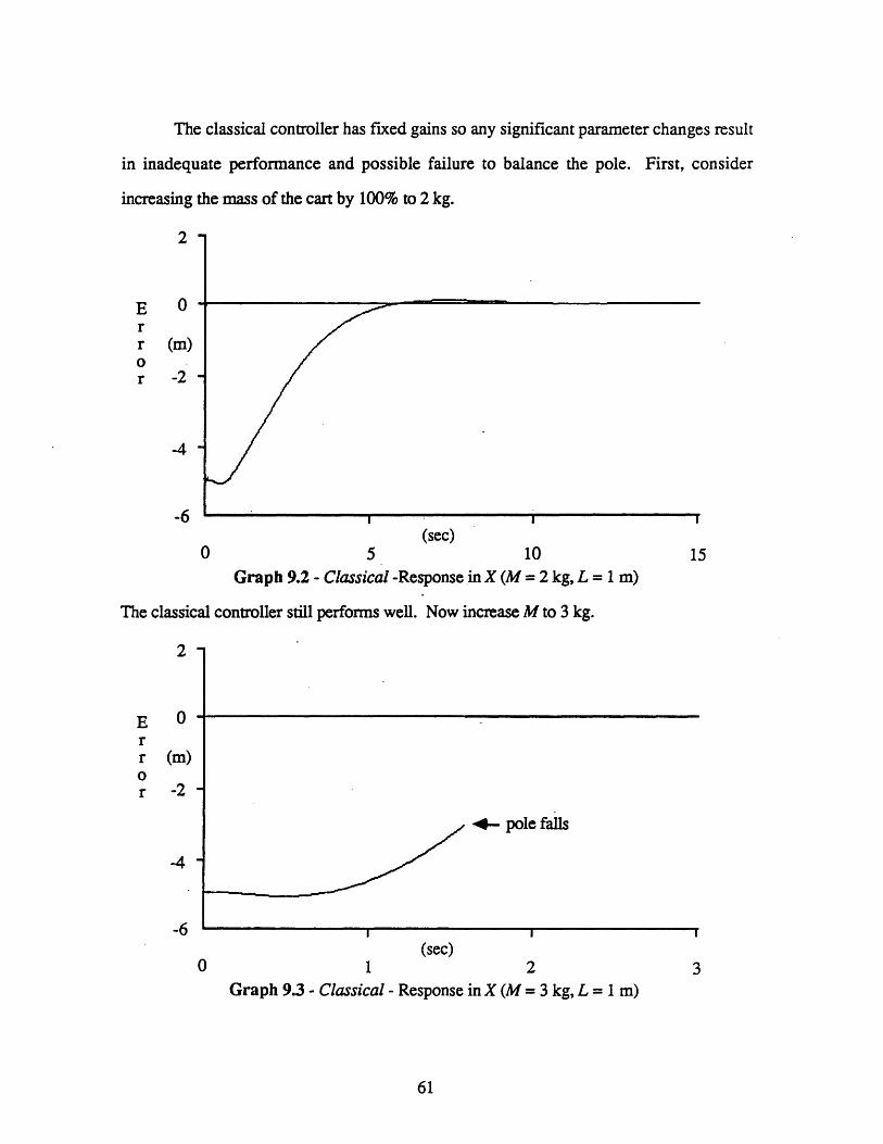
The classical controller has fixed gains so any significant parameter changes result

in inadequate performance and possible failure to balance the pole. First, consider

increasing the mass of the cart by 100% to 2 kg.

2

E 0rr (m)or -2

-4

-6(sec)

0 5 10

Graph 9.2 - Classical -Response in X (M = 2 kg, L = 1 m)

The classical controller still performs well. Now increase M to 3 kg.

E 0rr (m)or -2

-4

-6

0

15

4- pole falls

3

61

I I

(sec)1 2

Graph 9.3 - Classical - Response in X (M = 3 kg, L = 1 m)

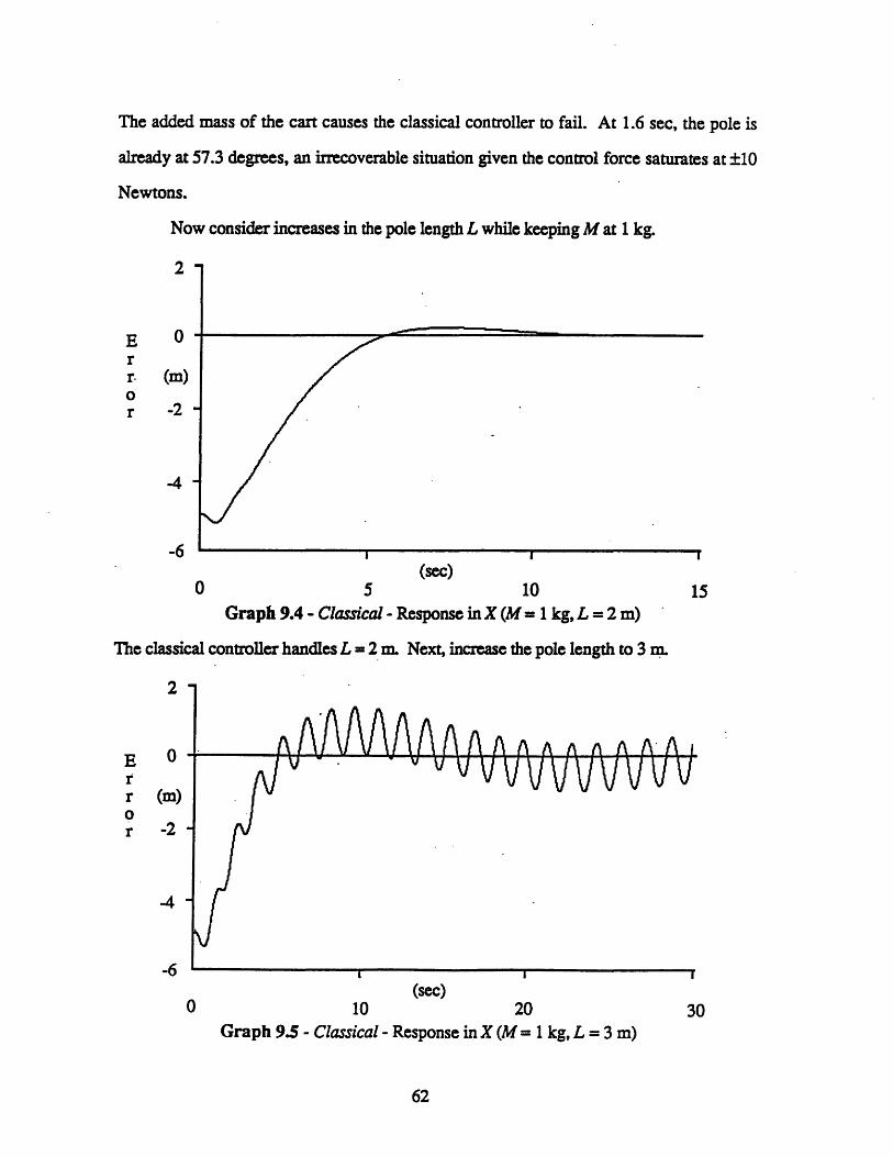
The added mass of the cart causes the classical controller to fail. At 1.6 sec, the pole is

already at 57.3 degrees, an irrecoverable situation given the control force saturates at ±10

Newtons.

Now consider increases in the pole length L while keeping M at 1 kg.

2

E 0rr (m)or -2

-4

-6(sec)

0 5 10

Graph 9.4 - Classical - Response inX (M = 1 kg, L = 2 m)

The classical controller.handles L = 2 m. Next, increase the pole length to 3 m.

15

AA AAAAAV v VvvU VVVV v

A A n n A A'A i

30

62

E 0-rr (m)O

r -2

-4-

-6

0

I I

(sec)10 20

Graph 9.5 - Classical - Response in X (M = 1 kg, L = 3 m)

w ........ *JF 0*0| |0| _ · · · · · I_··__··I _ _· r·_·l

ZI

The added length of the pole causes an oscillation (1.32 m peak-to-peak) and a substantially

longer settling time. Despite keeping the pole upright, the classical controller reveals severe

limitations at this parameter setting.

9.2 THE NEURAL NETWORK CONTROLLER

This section takes the neural network controller through a series of experiments

which illustrate distinct advantages over the classical controller. The first network

controller experiment called Linear-Initialization confirms that the interconnection weights

converge to a desired configuration. For this experiment, the weights are initialized using

the reference controller gains assuming the neurons operate in the linear region. The

network attempts to control a plant with dynamic parameters (M = 1 kg, L = 1 m) identical

to the model reference. To teach the network, the user gives the controller a string of 5 m

commands allowing for settling time in between. The superimposed graphs of the initial

network response and the reference response are almost the same, but the assumption of

linear neurons is not valid. After five commands, the weights converge to give a response

very close to the reference.

2

E 0rr (m)or -2

-4

-6

63

(sec)0 5 10 15

Graph 9.6 - Linear-Initialization - lst Response in X (M = 1 kg, L = 1 m)

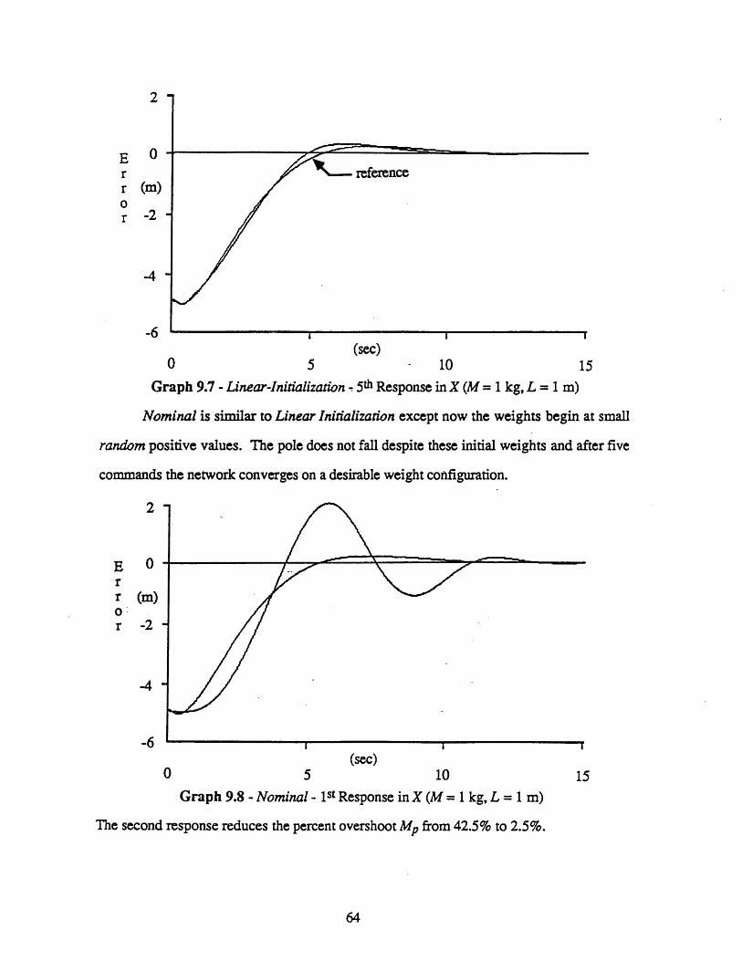
2

E 0rr (m)0r -2

-4

-6(sec)

0 5 10 15

Graph 9.7 - Linear-Initialization, 5th Response in X (M = 1 kg, L = 1 m)

Nominal is similar to Linear Initialization except now the weights begin at small

random positive values. The pole does not fall despite these initial weights and after five

commands the network converges on a desirable weight configuration.

2

E rr (m)0 r -2

-4

-6(sec)

0 5 10

Graph 9.8 - Nominal - 1St Response in X (M = 1 kg, L = 1 m)

The second response reduces the percent overshoot Mp from 42.5% to 2.5%.

15

64

2

E 0rr (m)or -2

-4

-6

reference

(sec)0 5 - 10 15

Graph 9.9 - Nominal - 2nd Response inX (M = 1 kg, L = 1 m)

Finally, the fifth response has an overshoot of 4.3% compared to the reference Mp of

4.4%.

2

E 0rr(m)or -2

-4

-6(sec)

0 5 10 15

Graph 9.10 - Nominal - 5th Response in X (M = 1 kg, L = 1 m)

Linear Big M uses the initial weights in the Linear Initialization experiment but now

the cart mass is set to 3 kg. The classical controller fails to keep the pole upright with this

parameter setting. The network also fails to balance the pole on the first two tries.

65

2

E 0rr(m)0r -2

-4

-6(sec)

0 2.5 5 7.5

Graph 9.11 - Linear Big M - 1st and 2nd Response inX (M = 3 kg, L = 1 m)

The network controller keeps the pole upright on the third response, but the curve diverges

from the reference in its early stages.

2

E 0rr (m)or -2

-4

-6(sec)

0 5 10

Graph 9.12 - LinearBig M- 3rd Response inX (M = 3 kg, L = 1 m)

An intermediate fifth response shows good progress in following the reference,

15

66

-

2

E 0rr (m)or -2

-4

-6

reference

(sec)0 5 10

Graph 9.13 - Linear Big M- 5th Response in X (M = 3 kg, L = 1 m)

and eventually the weights settle to give a good seventh response.

Z

E 0rr (m)or -2

-4

-6

15

(sec)0 5 10 15

Graph 9.14 - Linear Big M - 7 th Response in X (M = 3 kg, L = 1 m)

Random Big M uses random initial weights as in the Nominal experiment with a

cart mass of 3 kg. The network fails to balance the pole on the first try after overshooting

the desired cart position by 170.0%.

67

8

4

E 0 -rr (m)0o

r -4-

o

4- pole falls

-o , i

(sec)0 2.5 5 7.5

Graph 9.15 - Random Big M - 1St Response in X (M = 3 kg, L = 1 m)

The pole also falls in the second response after the cart overshoots Xc by 52.5% and

overcompensates on the recovery.

8

4-

E 0rr (m)or -4

-Q

\- pole falls

-u I I I

(sec)0 5 10 15

Graph 9.16 - Random Big M- 2nd Response in X (M = 3 kg, L = 1 m)

The third response successfully reaches the desired cart position with an Mp of 24.5% and

a settling time 1.5 sec longer than the reference response

68

- - s ^ s s

2

E 0rr (m)0r -2

-4

-6(sec)

0 5 10 15

Graph 9.17 - Random Big M- 3rd Response in X (M = 3 kg, L = 1 m)

The weights eventually settle to give a tenth response that closely follows the reference.

2

E 0rr (m)or -2

-4

-6(sec)

0 5 10 15

Graph 9.18 - Random Big M - 10th Response in X (M = 3 kg, L = 1 m)

Linear Big L begins with an initial linear guess for the weights and attempts to

balance a cart-pole with an M of 1 kg and an L of 3 m. With these settings the classical

controller experiences a slow settling time with a large oscillation (1.32 m peak-to-peak)

69

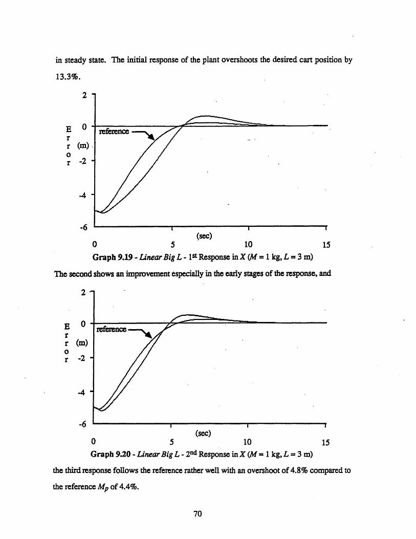
in steady state. The initial response of the plant overshoots the desired cart position by

13.3%.

2

E Orr (m)or -2

-4

-6(sec)

0 5 10 15

Graph 9.19 - Linear Big L - 1t Response in X (M = 1 kg, L = 3 m)

The second shows an improvement especially in the early stages of the response, and

2

E 0rr (m)0r -2

-4

-6(sec)

0 5 10 15

Graph 9.20 - Linear Big L - 2nd Response in X (M = 1 kg, L = 3 m)

the third response follows the reference rather well with an overshoot of 4.8% compared to

the reference Mp of 4.4%.

70

2

E 0rr (m)or -2

-4

-6(sec)

0 5 10 15

Graph 9.21 - Linear Big L - 3rd Response in X (M = 1 kg, L = 3 m)

Finally, the fourth response mimics the reference despite a larger dip at the beginning due

to the increased pole length.

2

E 0rr (m)or -2

-4

-6(sec)

0 5 10 15

Graph 9.22 - Linear Big L - 4th Response in X (M = 1 kg, L = 3 m)

Random Big L begins with small random weights and attempts to balance the cart-

pole with an M of 1 kg and an L of 3 m. The cart-pole overshoots the desired position on

the first response by 41.5%.

71

2

E 0rr (m)or -2

-4

-6(sec)

0 5 10

Graph 9.23 - Random Big L - 1St Response in X (M = 1 kg, L = 3 m)

The second response decreases the overshoot to 11.3%, and

E Orr (m)

r -2

-4

-6(sec)

0 5 10

Graph 9.24 - Random Big L - 2nd Response in X (M = 1 kg, L = 3 m)

the third response almost duplicates the reference.

72

15

15

2

E 0rr (m)0r -2

-4

-6

reference

(sec)0 5 10 15

Graph 9.25 - Random Big L - 3rd Response in X (M = 1 kg, L = 3 m)

After only four position commands to the cart-pole, the network controller learns to imitate

the response of the reference.

2

E 0rr (m)0r -2

-4

-6(sec)

0 5 10 15

Graph 9.26 - Random Big L - 4th Response in X (M = 1 kg, L = 3 m)

The last experiment, Big Xc, demonstrates the thresholding effects of the neurons

for large commanded cart positions. After Linear Initialization converges on a set of

weights, the cart is commanded to 10 m. For any Xc larger than 5 m, the classical

73

controller must use limiters on Oc to keep the pole balanced. The network controller relies

only on the thresholding characteristics of the neurons.

4

E Orr (m)0r -4

-8

-12(sec)

0 5 10 15

Graph 9.27 - Big Xc- Response in X (M = 1 kg, L = 1 m)

3 SUMMARY OF THE RESULTS

Each of these experiments highlights an important capability of the network

controller. In general, an experiment takes less than ten commands to converge on a good

set of weights, and often the plant and reference responses are close after only two or three

commands. The network typically converges quicker with an initial linear guess of the

weights than with originally random weights.

The following two tables summarize the results of the experiments that started with

random weights. A measure of similarity between the plant and reference responses is the

difference in percent overshoot Mp. For all the experiments, the network controller

attempts to duplicate the target overshoot of 4.4% of the reference response. Table 9.1

displays the results of the experiments where M was increased and L remained at 1 m. A

"*" indicates the network controller failed to balance the pole.

74

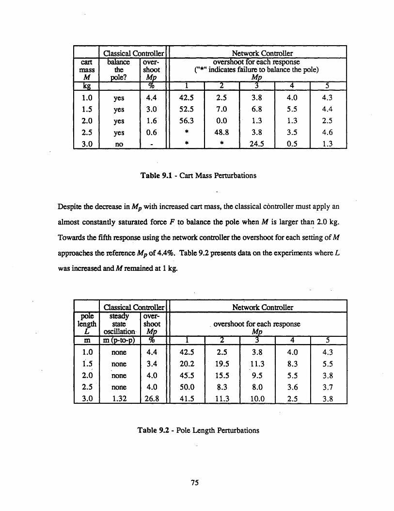
Table 9.1 - Cart Mass Perturbations

Despite the decrease in Mp with increased cart mass, the classical controller must apply an

almost constantly saturated force F to balance the pole when M is larger than 2.0 kg.

Towards the fifth response using the network controller the overshoot for each setting of M

approaches the reference Mp of 4.4%. Table 9.2 presents data on the experiments where L

was increased and M remained at 1 kg.

Table 9.2 - Pole Length Perturbations

75

Classical Controller Network Controllercart balance over- overshoot for each responsemass the shoot ("*" indicates failure to balance the pole)M pole? Mp Mp

kg % 1 2 3 4 5

1.0 yes 4.4 42.5 2.5 3.8 4.0 4.3

1.5 yes 3.0 52.5 7.0 6.8 5.5 4.4

2.0 yes 1.6 56.3 0.0 1.3 1.3 2.5

2.5 yes 0.6 * 48.8 3.8 3.5 4.6

3.0 no - * * 24.5 0.5 1.3

Classical Controller Network Controllerpole steady over-

length state shoot . overshoot for each responseL oscillation Mp MPm m(p-to-p) 1 1 2 3 4 5

1.0 none 4.4 42.5 2.5 3.8 4.0 4.3

1.5 none 3.4 20.2 19.5 11.3 8.3 5.5

2.0 none 4.0 45.5 15.5 9.5 5.5 3.8

2.5 none 4.0 50.0 8.3 8.0 3.6 3.7

3.0 1.32 26.8 41.5 11.3 10.0 2.5 3.8

At L larger than 2.0 m the classical controller waves the pole back and forth before settling

on the commanded cart position. At L = 3.0 m the classical controller fails to reach the

commanded position due to a severe oscillation in steady state. All of the fifth responses

for the network controller show an Mp close to the target value of 4.4%.

The final weights of the experiment offer important insight into the operation of the

neural network controller. Since the network configuration contains six adjustable weights

(see Figure 9.1) and the compensator for the cart-pole only requires 4 gains, there is not a

unique set of desired weights. Forpropagation attempts to "smear" the information of a

four-gain compensator into six weights.

0

X

x

W3 5

F

9

Figure 9.1 - Network Configuration

Table 9.3 shows the final value of the weights for some of the experiments.

76

initialL M weights Wei hts After Convergence

m kg w13 w14 w23 w24 w35 w45

1.0 1.0 linear 0.73 0.63 0.61 0.52 1.02 0.65

1.0 1.0 random 0.47 0.51 0.47 0.65 1.00 0.66

1.0 3.0 linear 0.61 0.55 0.60 0.57 1.12 0.56

1.0 3.0 random 0.51 0.57 0.41 0.35 1.21 0.91

3.0 1.0 linear 0.64 0.63 0.52 0.54 1.29 0.85

3.0 1.0 random 0.67 0.64 0.57 0.51 1.28 0.94

Table 9.3 - Network Weights

As the cart mass M or the pole length L increases, w35 and w45 consistently converge to

larger values. This suggests the network controller learns to quickly adjust to small

deviations in 0 and when the plant dynamics make it more difficult to balance the pole.

77

10 RECOMMENDATIONS AND CONCLUSIONS

The neural network controller performs well under the various exercises of

Chapter 9. This demonstrates the ability of forpropagation to seek and maintain weight

configurations capable of controlling the cart-pole in various operating envelopes. Section

10.1 presents closing comments on the experiments and general statements on the findings

of this research. Work in this field is far from complete and Section 10.2 offers some new

avenues of investigation to pursue.

10.1 CONCLUSIONS

The first experiment, Linear-Initialization, confirmed the stability of the

forpropagation algorithm. As the network controller approached the response of the

reference, the weights adjusted less dramatically and any small changes over later

responses integrated out to near zero. Nominal demonstrated the ability of the network

controller to learn a good weight configuration given no prior knowledge. Positive results

insured the gradient search technique invoked by forpropagation would work even with

initial weights far from the target. Linear Big M and Linear Big L showed the network

controller surpassing the capabilities of the fixed-gain classical controller in the presence of

a large change in cart mass or pole length. However, the weights for these experiments

began with a linear guess giving the network important initial information. Finally, in the

Nominal Big M and Nominal Big L experiments, the network controller outperformed the

classical controller given no prior knowledge.

Big Xc revealed the effect of the non-linear neurons in the network. After the

weights converged in the Linear-Initialization experiment, the cart-pole was commanded to

10 m, a task the classical controller would rely on limiters to perform. The network

78

controller, with the aid of the non-linear neurons, did not command a pole angle greater

than 15 degrees and moved the cart to the desired position. This result shows that limiting

effects, artificially produced in the classical controller, are naturally inherent in the network

controller.

The network inner-outer loop infrastructure proved essential for a successful

controller. The first layer received X - Xc and X and passed commanded positions for 0

and to the second layer. This separation of layers by inner and outer loop construction

can be used in many applications where this assumption is valid. Due to this infrastructure,

the network contained six adjustable weights as opposed to the four gains of the reference

controller. The network used this redundancy to "smear" the knowledge of the controller

into six weights. This common property of neural networks builds weight configurations

that allow small contributions from all neurons.

Overall, the forpropagation algorithm teamed with the network structure

accomplished tasks a similar network taught using backpropagation could not perform.

The forpropagation teaching sessions did not require any initial knowledge but merely a

reference to show the general response. Furthermore, the plant was only tracked in X and

X allowing 0 and to take on any time responses necessary. The action of the pole

over a response to a commanded cart position can vary greatly depending on the pole length

and cart mass. In the Big M and Big L experiments, the commanded pole positions were

modest compared to the classical controller.

10.2 RECOMMENDATIONS FOR FURTHER WORK

Through the course of this work, two important fields of study related to network

controllers were identified but not investigated thoroughly. All previous experiments

assumed full use of state variables, but Section 10.2.1 suggests a new approach to

implement partial-state feedback for the cart-pole controller. Section 10.2.2 presents the

79

idea of adjusting the reference to always insure peak system performance.

10.2.1 Partial-State Feedback Controllers

The architectures for partial-state feedback controllers closely resemble their full-

state counterparts but require memory to estimate the unavailable state variables.

Consequently, these controllers use one-step propagation which allows values from two

time steps to be differenced to estimate a velocity for the cart or pole. First, this section

considers the network that merely balances the pole. A value for the pole velocity is

estimated by differencing two pole positions over time. After determining , the

controller looks similar to the full-state version with two weighted inputs summed at the

output neuron to arrive at a control action F.

e- 0 c

Figure 10.1 - Proposed Network Structure of Partial-State 0 Controller

The partial-state X controller, which balances the pole while regulating the cart

position, cascades two triangular forms of the partial-state 0 controller. The first neuron

triad receives X - Xc and differences previous inputs to arrive at an estimate for X.

Signals proportional to X and X are then multiplied by weights and summed at an

intermediate linear neuron. This linear neuron also receives 0 and outputs a value

80

97

proportional to 0- Oc to the next triad of neurons. Again, differencing gives an estimate of

. The final control action is a function of - Oc and multiplied by weights.

X -X 4

Figure 10.2 - Proposed Network Structure of Partial-State X Controller

This architecture, though slightly more complicated than the full-state feedback network,

implements the same representation assuming the differencing operation is relatively

accurate.

10.2.2 Adjustable Reference

For all experiments the reference remained the same. This was adequate to prove

convergence qualities and performance capabilities of the forpropagation algorithm.

However, a new approach that adjusts the reference can maintain optimal performance in all

operating environments. If the dynamic problem becomes simpler, then the control action

F could give a better response than the current reference. An algorithm could make small

adjustments to the reference depending on a time history of the control action. If F rarely

peaks, the reference response can be improved and a full range of control action can yield a

better response. However, if F is constantly saturating and the network controller is

struggling, the reference response can be slightly degraded.

81

.4r

APPENDIX

The appendix contains the important source code listings of the neural network

simulator. The three programs, Pole-Exec, Forprop, and Pole-Dynamics, do not represent

all of the code necessary for the simulator. Various programs dealing only with graphics,

support routines, or simple utility functions do not appear. This section provides the top-

level and critical lower-level routines for the simulator.

A. 1 POLE-EXEC.LISP

Pole-Exec runs the top-level loop of the simulator and handles all operations on

experiments. The user can create, stop, run, and reset the experiments defined in this

program.

POLE-EXEC FLAVOR

(defflavor pole-exec((process)

(process-run-f)(net-type)(net)

(dynamics (make-instance 'pole-state))(teacher (make-instance 'teacher))(network-pane)(pane-b)(phase-pane)(menu-pane)(duration-pane)(cart-pane)

(keyboard-io-pane)(network-pane-update-f t)

(pane-b-update-f t)

(phase-pane-update-f nil)(phase-pane-x-abs 7)

82

(phase-pane-y-abs 7)

(duration-pane-update-f t)

(duration-pane-update-inc-f t)

(cart-pane-update-f nil)(discrete-f t)

(lesson 0)

(count 0)

(suspend-f)(scale 1.0)

(scale-exp -.005)(grade 0.0)

(total-count 0)

(final-count 3000)(neuron-update-f)(neuron-on-display)(old-circle-data nil)

(pathname "M :>bes>test.lisp")(banner "this is a test"))

0:initable-instance-variables:writable-instance-variables)

POLE-EXEC METHODS

(defmethod (run-experiment pole-exec) (controller)(if process

(mom-menu "Experiment Already Running, Big Dummy" '(nil "Abort" nil))

(progn

(setq process-run-f t)

(setq process

(process-run-function "Neural Loop Process" 'run-loop self)))))

(defmethod (stop-experiment pole-exec) ()

(cond (process-run-f(setq process-run-f nil)

(si:process-sleep 120)

(setq process nil))

(t (mom-menu "No Experiment Is Running" '(nil "Abort" nil)))))

(defmethod (reset-experiment pole-exec) ()(if process-run-f (stop-experiment self))

(setq lesson 0)

(setf (pole-state-lesson dynamics) 0)(setq suspend-f nil)

83

(initialize-weights net)

(balance dynamics)(balance (pole-state-reference dynamics))(setf (pole-state-time dynamics) 0.0)(seff (pole-state-desired-x dynamics) 0.0)(seff (pole-state-time (pole-state-reference dynamics)) 0.0)(setq neuron-update-f nil)(cond-every(pane-b-update-f(init pane-b))

(network-pane-update-f(init network-pane net)).

((not (pole-state-clascon-f dynamics))(int phase-pane)(setf phase-pane-update-f nil)))

(init duration-pane net)

(init cart-pane dynamics))

BLIP READER METHODS

(defmethod (loop-net-blip-reader pole-exec) ()(loop do (handle-neuron-click self (send network-pane :any-tyi))))

(defmethod (handle-neuron-click pole-exec) (blip)(if (listp blip)

(if (> (length blip) 2)

(if (eq (car blip) 'typeout-execute)(cond ((or (= (second blip) 0) ( (second blip) 1))

(setq neurn-on-display (car (third blip)))

(if oldcircle-data

(parn(send network-pane ':draw-filled-in-circle

(first old-cire-data)

(second old-circle-data)

(third old-circle-data)

tvalu-andca)

(send network-pane ':draw-circle

(first old-cirdcle-data)

(second old-circle-data)

(third old-circle-data))))

(send network-pane ':draw-filled-in-circle

(second (third blip))

(third (third blip))

(fourth (third blip)))

84

(setq old-circle-data (cdr (third blip)))

(show-weight neuron-on-display pane-b)

(setq neuron-update-f (= 0 (second blip))))

((= 2 (second blip)) (change-neuron (car (third blip))))

((= 3 (second blip))

(if old-circe-data

(send network-pane ':draw-filled-in-circle ;erase black circle

(frst old-ccle-data)(second old-circle-data)

(third old-circle-data)

tvalu-andca)

(send network-pane ':draw-circle ;redraw white circle

(first old-circleata)

(second oldcircle-data)

(third old-circle-data))

(setq old-circledata nil)))(setq neuron-on-display (network-threshold net))

(show-weight neuron-on-display pane-b)

(setq neuron-update-f t)))))))

MAIN EXECUTION LOOP

(defmethod (run-loop pole-exec) ()(send network-pane :set-io-buffer (tv:make-io-buffer 1024))(send network-pane :select)(if (pole-state-write-stats-f dynamics)

(append-to-streams'(,pathname) banner))(loop while process-run-f

do

(cond ((not suspend-f)

(setq lesson (1+ lesson))

(setf (pole-state-lesson dynamics) (1+ (pole-state-lesson dynamics).))(if (member (plot-pane-plot-type duration-pane) '(2 3))

(init duration-pane net))

(setq count 0)

(setf (pole-state-duration dynamics) 0)

(balance dynamics)

(balance (pole-state-reference dynamics))

(set-kick dynamics

(* (pole-state-initial-kick dynamics) (if (zerop (mod lesson 2)) -1 1)))

(set-kick (pole-state-reference dynamics)

(* (pole-state-initial-kick dynamics) (if (zerop (mod lesson 2)) -1 1)))

(setq scale 1.0))

85

(t (setq suspend-f nil)))

(loop while (and process-run-f(not (funcall (teacher-trip-function teacher) dynamics)))

do

(setq count (1 + count))

(seff (pole-state-duration dynamics) (* count (pole-state-dt dynamics)))(if (and (pole-state-write-stats-f dynamics)

(zerop (mod count (pole-state-write-stats-frequency dynamics))))

(append-to-streams '(,pathname)"-% time = -2,2,6$ x-comrn = -2,2,6$ kick = 2,2,6$-%

theta = -2,2,6$ thetad = -2,2,6$ x ="

(pole-state-time dynamics)

(pole-state-desired-x dynamics)

(pole-state-kick dynamics)

(pole-state-theta dynamics)

(pole-state-thetad dynamics)

(pole-state-x dynamics)

(pole-state-xd dynamics)))

(if cart-pane-update-f

(update cart-pane cart-pane dynamics))

(if phase-pane-update-f(update phase-pane (pole-state-theta dynamics) (pole-state-thetad dynamics)

(/ (pole-state-kick dynamics) 10.0)))

(zl:selectq (plot-pane-plot-type duration-pane)(1 (update duration-pane lesson (* count (pole-state-dt dynamics))))(2 (update duration-pane (* count (pole-state-dt dynamics))

(- (pole-state-x dynamics) (pole-state-desired-x dynamics))))

(3 (update duration-pane (* count (pole-state-cdt dynamics))

(- (pole-state-x dynamics) (pole-state-desired-x dynamics))

(* count (pole-state-dt dynamics))

(- (pole-state-x (pole-state-reference dynamics))

(pole-state-desired-x (pole-state-reference dynamics))))))

(handle-neuron-click self (send network-pane :any-tyi-no-hang))(if neuron-update-f (update pane-b neuron-on-display))(cond ((pole-state-clascon-f dynamics)

(if (pole-state-time-fudge-f dynamics) (cl:sleep 0.04))

(update dynamics)

(set-kick dynamics (clascon dynamics)))

(t

(update dynamics)

(update (pole-state-reference dynamics) dynamics)

(evaluate dynamics net scale)

(if (teacher-teacher-on-f teacher) (teach teacher net dynamics))

(propagate net (process-inputs dynamics))

(set-kick dynamics (* 10.0 (first (get-outputs net))))

(set-kick (pole-state-reference dynamics)

86

(clascon (pole-state-reference dynamics) dynamics))))

finally

(if (and process-run-f duration-pane-update-f)

(zl:selectq (plot-pane-plot-type duration-pane)(1 (update duration-pane lesson (* count (pole-state-dt dynamics))))

(2 (update duration-pane (* count (pole-state-dt dynamics))

(- (pole-state-x dynamics) (pole-state-desired-x dynamics))))

(3 (update duration-pane (* count (pole-state-dt dynamics))

(- (pole-state-x dynamics) (pole-state-desired-x dynamics))

(* count (pole-state-dt dynamics))

(- (pole-state-x (pole-state-reference dynamics))

(pole-state-desired-x (pole-state-reference dynamics))))))

(if (not process-run-f) (setq suspend-f t))

(send keyboard-io-pane :select)))))

EXPERIMENTS

(defmethod (create-experiment-menu pole-exec) ()(zl:selectq (mom-menu "Choose Experiment"

'(nil

"Theta and x Classical Controller"

"Layered x - fpr - linear-initialization"

"Layered x - fpr - nominal""Layered x - fpr - linear big M"

"Layered x - fpr - nominal big M"

"Layered x - fpr - linear big L""Layered x -fpr - nominal big L"

nio)

(1 (setq net

(create-network

'((1 input neuron2 (3.0)) (1 output neuron2 (5.0)))

'((Ho4- 0 1))

'((net nil nil uniform (0.0 0.3)))

'propagate-feedforward))

(seff (network-experiment-name net) " Theta and x Classical Controller')(send network-pane :clear-window)

(setq network-pane-update-f nil)

(send pane-b :clear-window)

(setq pane-b-update-f nil)

(send phase-pane :clear-window)

(setq phase-pane-update-f nil)

(seff (pole-state-clascon-f dynamics) t))

87

(2 (setq net

(create-network

'((2 input neuron2 (2.0 1.0)) (2 hidden neuron2 (2.0 1.0))

(1 output neuron2 (2.0)))

'((I-to-I 0 1) (-to- 1 2))

'((I-to-l-custom 0 1 nil ((0.548 0.0) (0.670 0.0)))

(I-to-l-custom 1 2 nil ((1.216) (0.462))))

popagate-feedforward))(setf (network-experiment-name net)" Layered x - fpr - linear-initialization")(seff (pole-state-x-neuron dynamics) (nth 0 (network-sequentials net)))(setf (pole-state-xd-neuron dynamics) (nth 1 (network-sequentials net)))(seff (pole-state-theta-neuron dynamics) (nth 2 (network-sequentials net)))(seff (pole-state-thetad-neuron dynamics) (nth 3 (network-sequentials net)))(setf (pole-state-theta-continuous-scale dynamics) 8.0)(seff (pole-state-thetad-continuous-scale dynamics) 4.0)(seff (pole-state-x-continuous-scale dynamics) 0.30)(setf (pole-state-xd-continuous-scale dynamics) 0.90)(setf (pole-state-process-inputs-function dynamics)

layered-x)

(seff (pole-state-evaluate-function dynamics) 'evaluate-4ref)(setf (teacher-learning-coefficient teacher) 0.01)(setf (teacher-update-interval teacher) 5)(seff (teacher-teach-function teacher) Ipr))

(3 (setq net

(create-network

'((2 input neuron2 (2.0 1.0)) (2 hidden neuron2 (2.0 1.0))

(1 output neuron2 (2.0)))

'((I-to-l 0 1 )(-to 1 2))

'((-to-l 0 1 uniform (0.0 0.3))(I-to-I 1 2 uniform (0.0 0.3)))

propagate-feedforward))

(seff (network-experiment-name net)" Layered x - fpr - nominal")(seff (pole-state-x-neuron dynamics) (nth 0 (network-sequentials net)))(setf (pole-state-xd-neuron dynamics) (nth 1 (network-sequentials net)))(setf (pole-state-theta-neuron dynamics) (nth 2 (network-sequentials net)))(setf (pole-state-thetad-neuron dynamics) (nth 3 (network-sequentials net)))(setf (pole-state-theta-continuous-scale dynamics) 8.0)(setf (pole-state-thetad-continuous-scale dynamics) 4.0)(setf (pole-state-x-continuous-scale dynamics) 0.30)(seff (pole-state-xd-continuous-scale dynamics) 0.90)(seff (pole-state-process-inputs-function dynamics)

layered-x)

(seff (pole-state-evaluate-function dynamics) 'evaluate-4ref)(seff (teacher-learning-coefficient teacher) 0.01)(seff (teacher-update-interval teacher) 5)

88

(seff (teacher-teach-function teacher) pr))

(4 (setq net

(create-network

'((2 input neuron2 (2.0 1.0)) (2 hidden neuron2 (2.0 1.0))

(1 output neuron2 (2.0)))

'((I-to-I 01) (I-to-l 1 2))

'((I-to-l-custom 0 1 nil ((0.548 0.0) (0.670 0.0)))

(I-to-l-custom 1 2 nil ((1.216) (0.462))))

'propagate-feedforward))

(seff (network-experiment-name net)" Layered x - fpr - linear big M")(seff (pole-state-x-neuron dynamics) (nth 0 (network-sequentials net)))(seff (pole-state-xd-neuron dynamics) (nth 1 (network-sequentials net)))(seff (pole-state-theta-neuron dynamics) (nth 2 (network-sequentials net)))(seff (pole-state-thetad-neuron dynamics) (nth 3 (network-sequentials net)))(seff (pole-state-theta-continuous-scale dynamics) 8.0)(seff (pole-state-thetad-continuous-scale dynamics) 4.0)(seff (pole-state-x-continuous-scale dynamics) 0.30)(seff (pole-state-xd-continuous-scale dynamics) 0.90)(seff (pole-state-process-inputs-function dynamics)

layered-x)

(seff (pole-state-evaluate-function dynamics) 'evaluate-4ref)(seff (pole-state-mc dynamics) 3.0)

(seff (teacher-ieamingcoefficient teacher) 0.01)(seff (teacher-update-interval teacher) 5)(seff (teacher-teach-function teacher) pr))

(5 (setq net

(crate-nework'((2 input neuron2 (2.0 1.0)) (2 hidden neuron2 (2.0 1.0))

(1 output neuron2 (2.0)))

'((I-to-I 0 1) (I-to-I 1 2))

'((I-to-l 0 1 uniform (0.0 0.3))

(to- 1 2 uniform (0.0 0.3)))

propagate-feedforward))

(seff (network-experiment-name net)" Layered x - fpr - nominal big L")(seff (pole-state-x-neuron dynamics) (nth 0 (network-sequentials net)))(seff (pole-state-xd-neuron dynamics) (nth 1 (network.sequentials net)))(seff (pole-state-theta-neuron dynamics) (nth 2 (network-sequentials net)))

(seff (pole-state-thetad-neuron dynamics) (nth 3 (network-sequentials net)))(seff (pole-state-theta-continuous-scale dynamics) 8.0)(seff (pole-state-thetad-continuous-scale dynamics) 4.0)(seff (pole-state-x-continuous-scale dynamics) 0.30)(seff (pole-state-xd-continuous-scale dynamics) 0.90)(seff (pole-state-process-inputs-function dynamics)

layered-x)

89

(seff (pole-state-evaluate-function dynamics) 'evaluate-4ref)(seff (pole-state-mc dynamics) 3.0)(seff (teacher-learning-coefficient teacher) 0.01)(seff (teacher-halt-function teacher) 'haltl)(seff (teacher-update-interval teacher) 5)

(seff (teacher-teach-function teacher) Ypr))))

(6 (setq net

(create-network

'((2 input neuron2 (2.0 1.0)) (2 hidden neuron2 (2.0 1.0))

(1 output neuron2 (2.0)))

'((I-to-I 0 1) (I-to-l 1 2))

'((I-to--custom 0 1 nil ((0.548 0.0) (0.670 0.0)))

(I-to-l-custom 1 2 nil ((1.216) (0.462))))

'propagate-feedforward))

(seff (network-experiment-name net) " Layered x - fpr - linear big L")(seff (pole-state-x-neuron dynamics) (nth 0 (network-sequentials net)))(seff (pole-state-xd-neuron dynamics) (nth 1 (network-sequentials net)))(seff (pole-state-theta-neuron dynamics) (nth 2 (network-sequentials net)))(seff (pole-state-thetad-neuron dynamics) (nth 3 (network-sequentials net)))(seff (pole-state-theta-continuous-scale dynamics) 8.0)(seff (pole-state-thetad-continuous-scale dynamics) 4.0)(seff (pole-state-x-continuous-scale dynamics) 0.30)(seff (pole-state-xd-continuous-scale dynamics) 0.90)(seff (pole-state-process-inputs-function dynamics)

layered-x)

(seff (pole-state-evaluate-function dynamics) 'evaluate-4ref)(seff (pole-state-I dynamics) 1.5)

(seff (teacher-learning-coefficient teacher) 0.01)(seff (teacher-update-interval teacher) 5)

(seff (teacher-teach-function teacher) pr))

(7 (setq net

(create-network

'((2 input neuron2 (2.0 1.0)) (2 hidden neuron2 (2.0 1.0))

(1 output neuron2 (2.0)))

'((I-to-l 0 1) (I-to-I 1 2))

'((I-to-I 0 1 uniform (0.0 0.3))

(I-to-I 1 2 uniform (0.0 0.3)))

'propagate-feedforward))

(seff (network-experiment-name net)" Layered x - fpr - nominal big L")

(setf (pole-state-x-neuron dynamics) (nth 0 (network-sequentials net)))(seff (pole-state-xd-neuron dynamics) (nth 1 (network-sequentials net)))(seff (pole-state-theta-neuron dynamics) (nth 2 (network-sequentials net)))(seff (pole-state-thetad-neuron dynamics) (nth 3 (network-sequentials net)))(seff (pole-state-theta-continuous-scale dynamics) 8.0)

90

(serf (pole-state-thetad-continuous-scale dynamics) 4.0)(serf (pole-state-x-continuous-scale dynamics) 0.30)

(serf (pole-state-xd-continuous-scale dynamics) 0.90)(seff (pole-state-process-inputs-function dynamics)

layered-x)

(seff (pole-state-evaluate-function dynamics) 'evaluate-4ref)(seff (pole-state-l dynamics) 1.5)

(seff (teacher-learning-coefficient teacher) 0.01)(seff (teacher-halt-function teacher) 'haltl)(sef (teacher-update-interval teacher) 5)(serf (teacher-teach-function teacher) lpr))))

A.2 FORPROP.LISP

Forprop defines all flavors (data structures) and methods (functions on data

structures) related to neurons, networks, and teachers. The program contains routines to

create, propagate (complete or one-step), and teach (forpropagation or backpropagation) the

network

NEURON FLAVOR

(defflavor neuron(id-type

(actor'acivate-summer)outputter(internal-state 0.0)

(last-internal-state 0.0)

(external-state 0.0)

(last-external-state 0.0)

(error o.0)

(last-error 0.0)

mbdadynamic-sign

(max-sigmoid-input 10.0)

(min-sigmoid-input -1 0.0))

(node):initable-instance-variables

91

:writable-instance-variables)

(defflavor neuron1((outputter 'output-sigmoidl))(neuron)

:initable-instance-variables:writable-instance-variables)

(defflavor neuron2((outputter 'output-sigmoid2))(neuron)

:initable-instance-variables:writable-instance-variables)

(defflavor neuron-linear((outputter 'output-linear))(neuron)

:initable-instance-variables:writable-instance-variables)

NEURON METHODS

(defmethod (round-x-state neuronl) ((if (> extemal-state 0.5) 1 0))

(defmethod (round-x-state neuron2) ((if (> extemal-state 0.0) 1 0))

(defmethod (set-ex-state neuron) (ex-state)(serf last-external-state external-state)(serf extemal-state ex-state))

(defmethod (set-error neuron) (new-error)(setf last-error error)

(serf error new-error))

NEURON-TEACHERS

BACKPROPAGATION

92

(defmethod (teach-backprop-errors neuron) ()(setq error

(* (deriv-output-sigmoid self)(loop for neuron-alist in output-alist

for n = (first neuron-alist)

for weight = (cdr neuron-alist)

summing (* weight (neuron-error n))))))

(defmethod (teach-backprop-weights neuron) (from-neuron teacher)(let* ((old-weight (get-old-weight from-neuron self))

(weight (get-weight from-neuron self))(last-weight-change (- weight old-weight)))

(set-weight

from-neuron self (+ old-weight(+ (* (teacher-learning-coefficient teacher)

error (neuron-extemal-state from-neuron))

(* (teacher-momentum-coefficient teacher)

last-weight-change))))))

FORPROPAGATION

(defmethod (teach-forprop-errors neuron) ()(setq error

(* (deriv-output-sigmoid self)(loop for neuron-alist in input-alist

for n - (first neuron-alist)

for weight = (cdr neuron-alist)summing (* weight (neuron-error n))))))

(defmethod (teach-forprop-weights neuron) (from-neuron teacher)(let* ((old-weight (get-old-weight from-neuron self))

(weight (get-weight from-neuron self))(last-weight-change (- weight old-weight)))

(set-weight

from-neuron self (+ old-weight(+ (* (teacher-leaming-coefficient teacher)

(neuron-external-state from-neuron)

(neuron-error from-neuron))

(* (teacher-momentum-coefficient teacher)

last-weight-change))))))

FORPROPAGATION WITH REFERENCE (FPR)

93

(defmethod (teach-fpr-weights neuron) (to-neuron teacher)(let* ((old-weight (get-old-weight self to-neuron))

(weight (get-weight self to-neuron))(last-weight-change (- weight old-weight)))

(set-weightself to-neuron (+ old-weight

(+ (* (teacher-learning-coefficient teacher)(deriv-output-sigmoid self)

(deriv-output-sigmoid to-neuron)

error)

(* (teacher-momentum-coefficient teacher)

last-weight-change))))))

NEURON-INITIALIZERS

(defmethod (initialize neuron) (arglist)(setf lambda (first arglist))

(setf dynamic-sign (second arglist)))

NEURON-ACTIVATORS

(defmethod (activate-summer neuron) (&optional (ext-input 0.0))(let ((temp (+ (loop for input-neuron-alist in (node-input-alist self)

summing (* (cdr input-neuron-alist)

(neuron-external-state (first input-neuron-alist))))

ext-input)))

(sef last-internal-state internal-state)(setf internal-state temp)))

NEURON-OUTPUTTERS

(defmethod (output neuron) ()(funcall outputter self))

(defmethod (output-sigmoidl neuron) ()(setf last-external-state external-state)(setf external-state

(/1.0 (+ 1.0 (exp (min max-sigmoid-input

(max nin-sigmoid-input

94

(* -1.0 internal-state larrda))))))))

(defmethod (output-sigmoid2 neuron) ()

(self last-extemal-state external-state)(self external-state

(*2.0(-(/1.0 (+1.0

(exp (min max-sigmoid-input

(max min-sigmoidinput

( -1.0 internal-state lambda)))))) 0.5))))

(defmethod (output-linear neuron) ()(seff last-external-state external-state)(self external-state internal-state))

DERIVATIVE OUTPUT FUNCTIONS

(defmethod (deriv-output-sigmoid neuron) ()(funcalt (intem (string-append 'deriv- (neuron-outputter self))) self))

(defmethod (deriv-output-sigmoidl neuron) ()(* external-state (- 1.0 external-state)))

(defmethod (deriv-output-sigmoid2 neuron) ()(let ((val (exp (min max-sigmoid-input

(max min-sgmoid-input

-1.0 internalstate lambda))))))

( (* 2.0 lambda val) (square (+ 1.0 val)))))

NETWORK FLAVOR

(defflavor network

((irputs)(hiddens)

(outputs)

(threshold)

(sequentials)

(layers)

(teacher-list)creation-list

oonnection-list

weight-init-list

LIST OF NEURONS CONNECTED AS INPUTSLIST OF INTERNAL NEURONSLIST OF NEURON CONNECTED AS OUTPUTONE THRESHOLD NEURONDIRECTED LIST OF ALL NEURONSLIST OF LAYERSLIST OF TEACHER LOOPSDEFINES STRUCTURE OF NET (NEURONS)

DEFINES CONNECTIONS OF NEURONSDEFINES INITIAL CONNECTION WEIGHTS

95

teacher-init-list DEFINES HOW TO TEACH NET

propagator FULL OR ONE-STEP PROPAGATION FUNCTION

experiment-name)

0:initable-instance-variables:writable-instance-variables)

NETWORK METHODS

(defun create-network(creation-list connection-list weight-init-list propagator)

(let ((net (make-instance 'network:creation-list creation-list

:connection-list connection-list

weight-init-list weight-init-list

propagator propagator)))

(initialize net)

(connect net)

(initialize-weights net)

net))

(defun create-network-from-file (filename)(with-open-file (stream filename

:direction :input

:characers t)

(create-network(read stream)

(read stream)

(read stream)

(read stream)

(read stream))))

(defmethod (initialize network) ()(loop for layer-process-list in creation-list

for number-to-create = (first layer-process-list)

for id-type = (second layer-process-list)

for neuron-type = (third layer-process-list)for creation-args = (fourth layer-process-list)

do (if (equal id-type 'threshold)

(let ((new-neuron (make-instance neuron-type)))

(initialize new-neuron creation-args)

(serf (neuron-id-type new-neuron) id-type)

(seff threshold new-neuron))

(loop for n from 1 to number-to-create

96

for new-neuron = (make-instance neuron-type)

do (initialize new-neuron creation-args)

(self (neuron-id-type new-neuron) id-type)

(setf sequentials(append sequentials (list new-neuron)))

collecting new-neuron into layer-list

finally (let ((layer (create-layer layer-list)))

(setf layers (append layers (list layer)))

(cond ((equal id-type 'input)

(setf inputs layerist))

((equal id-type 'hidden)

(self hiddens (append hiddens (list layer-list))))

((equal id-type 'output)

(seff outputs layer-lst))))))))

(defmethod (connect network) ((loop for connection in connection-list

for conn = (first connection)for from-num - (second connection)for to-num = (third connection)do (cond ((equal conn 'I-to-l)

(connect (nth from-num layers) (nth to-num layers)))

((equal conn I-to-net)

(loop for neuron-to in sequentials

do (connect threshold neuron-to)))

((equal conn 'n-to-n)

(connect (nth from-num sequentials) (nth to-num sequentials)))

((equal conn 'n-to-I)

(connect-node-to-layer (nth from-num sequentials) (nth to-num layers)))

((equal onn 'l-to-n)

(connect-layer-to-node (nth from-num layers) (nth to-num sequentials))))))

(defmethod (initialize-weights network) )(loop for weight-init in weight-init-list

for type = (first weight-init)for from-num - (second weight-init)for to-num - (third weight-init) -for weight-func - (intern (string-append 'initialize-weights- (fourth weight-init)))for weight-func-args = (fifth weight-init)do (cond ((equal type 'net)

(loop for neuron in sequentials

do (loop for output-neuron-alist in (node-output-alist neuron)

for output-neuron = (first output-neuron-alist)

do (set-weight neuron output-neuron

(funcal weight-func weight-func-args) t))))((equal type 'net-t)

97

(loop for neuron in (append sequentials (list threshold))do (loop for output-neuron-alist in (node-output-alist neuron)

for output-neuron = (first output-neuron-alist)

do (set-weight neuron output-neuron

(funcall weight-func weight-func-args) t))))

((equal type 'net-t-custom)

(loop for neuron in (append sequentials (list threshold))for weight-list in weight-func-args

do (loop for output-neuron-alist in (node-output-alist neuron)

for output-neuron = (first output-neuron-alist)

forweight in weight-list

do (set-weight neuron output-neuron weight t))))

((equal type 1-to-l)

(let ((from-layer (nth from-num layers))

(to-layer (nth to-num layers)))

(loop for from-neuron in (layer-nodes from-layer)

do (loop for to-neuron in (layer-nodes to-layer)

do (if (assoc to-neuron (node-output-alist from-neuron))

(set-weight

from-neuron to-neuron

(funcall weight-func weight-func-args) t))))))

((equal type 1-to-I-custom)

(let ((from-layer (nth from-num layers))

(to-layer (nth to-num layers)))

(loop for from-neuron in (layer-nodes from-layer)

for weight-list in weight-func-args

do (loop for to-neuron in (layer-nodes to-layer)

for weight in weight-list

do (set-weight from-neuron to-neuron weight t))))))))

NETWORK PROPAGATORS

(defmethod (propagate network) (input-values)(funcall propagator self input-values))

(defmethod (propagate-feedforward network) (input-values)(if threshold (set-ex-state threshold 0.1))(loop for nlayer from 0

for neuron-list in (append (list inputs) hiddens (list outputs))

do (loop for nneuron from 0for neuron in neuron-list

do (let ((ext-input (nth nneuron (nth nlayer input-values))))

(if ext-input

(activate-summer neuron ext-input)

98

(activate-summer neuron))

(output neuron)))))

(defmethod (propagate-feedforward-step network) (input-values)(if threshold (set-ex-state threshold 0.1))(loop for nlayer from (1- (length layers))

for neuron-list in (append (list outputs) hiddens (list inputs))do (loop for nneuron from 0

for neuron in neuron-list

do (let ((ext-input (nth nneuron (nth nlayer input-values))))

(if ext-input

(activate-summer neuron ext-input)

(activate-summer neuron))

(output neuron)))))

NETWORK BACKPROP METHODS

(defmethod (teach-backprop-errors network) ()(loop for neuron-list in (zl:reverse hiddens)

do (loop for neuron in neuron-listdo (teach-backprop-errors neuron))))

(defmethod (teach-backprop-weights network) (teacher)(if threshold

(loop for to-neuron-alist in (node-output-alist threshold)for to-neuron - (first to-neuron-alist)do (teach-backprop-weights to-neuron threshold teacher)))

(loop for from-neuron-list in (append (list inputs) hiddens)do (loop for from-neuron in from-neuron-list

do (loop for to-neuron-alist in (node-output-alist from-neuron)

for to-neuron = (first to-neuron-alist)

do (teach-backprop-weights to-neuron from-neuron teacher)))))

NETWORK FORPROP METHODS

(defmethod (teach-forprop-errors network) ()(loop for neuron-list in (append hiddens (list outputs))

do (loop for neuron in neuron-listdo (teach-forprop-errors neuron))))

(defmethod (teach-forprop-weights network) (teacher)(if threshold

99

(loop for to-neuron-alist in (node-output-alist threshold)for to-neuron = (first to-neuron-alist)

do (teach-forprop-weights to-neuron threshold teacher)))(loop for from-neuron-list in (append (list inputs) hiddens)

do (loop for from-neuron in from-neuron-listdo (loop for to-neuron-alist in (node-output-alist from-neuron)

for to-neuron = (first to-neuron-alist)

do (teach-forprop-weights to-neuron from-neuron teacher)))))

NETWORK FPR METHODS

(defmethod (teach-fpr-weights network) (teacher)(loop for neuron-list in (append (list inputs) hiddens)

do (loop for from-neuron in neuron-listdo (loop for to-neuron-alist in (node-output-alist from-neuron)

for to-neuron = (first to-neuron-alist)

do (teach-fpr-weights from-neuron to-neuron teacher)))))

GENERAL NETWORK METHODS

(defmethod (get-outputs network) ()(loop for neuron in outputs

collecting (neuron-external-state neuron)))

(defmethod (get-rounded-outputs network) ()(loop for neuron in outputs

collecting (round-x-state neuron)))

(defmethod (get-externals-of-layer network) (nlayer)(loop for neuron in (layer-nodes (nth nlayer layers))

collecting (neuron-external-state neuron)))

(defmethod (get-intemals-of-layer network) (nlayer)(loop for neuron in (layer-nodes (nth nlayer layers))

collecting (neuron-intemal-state neuron)))

(defmethod (get-errors-of-layer network) (nlayer)(loop for neuron in (layer-nodes (nth nlayer layers))

collecting (neuron-error neuron)))

(defmethod (set-output-error-with-actual-desired network) (actual-values desired-values)(loop for output-neuron in outputs

100

for actual-value in actual-valuesfor desired-value in desired-valuesfor x-state = (neuron-external-state output-neuron)do (set-error output-neuron (* (deriv-output-sigmoid output-neuron)

(- desired-value actual-value)))))

(defmethod (set-input-error-with-actual-desired network) (actual-values desired-values)(loop for input-neuron in inputs

for actual-value in actual-values

for desired-value in desired-valuesfor x-state = (neuron-external-state input-neuron)

do (set-error input-neuron (* (deriv-output-sigmoid input-neuron)(- desired-value actual-value)))))

(defmethod (set-output-error-with-error network) (errors)(loop for output-neuron in outputs

for error in errors

do (seff (neuron-error output-neuron) (* (deriv-output-sigmoid output-neuron) error))))

(defmethod (set-input-error-with-error network) (errors)(loop for input-neuron in inputs

for error in errors

do (seff (neuron-error input-neuron) (* (deriv-output-sigmoid input-neuron) error))))

(defmethod (set-input-and-threshold-error-with-error network) (errors)(loop for input-neuron in (append inputs (list threshold))

for error in errors

do (seff (neuron-error input-neuron) (* (deriv-output-sigmoid input-neuron) error))))

(defmethod (calc network) (input)(propagate self input)(get-outputs self))

TEACHER FLAVOR

(defflavor teacher((teach-function)

(teacher-on-f t)

(learning-coefficient 0.1)

(momentum-coefficient 0.9)

(update-interval 1)

(update-count 0)

(trip-function 'simple-trip)

(halt-function 'no-halt))

101

0:initable-instance-variables:writable-instance-variables)

TEACHER METHODS

(defmethod (teach teacher) (network dynamics)(cond (teacher-on-f

(setq update-count (1+ update-count))(if ( 0 (mod update-count update-interval))

(if (not (funcall halt-function dynamics))

(funcall teach-function self network))))))

(defmethod (backprop teacher) (network)(teach-backprop-errors network)(teach-backprop-weights network self))

(defmethod (forprop teacher) (network)(teach-forprop-errors network)(teach-forprop-weights network self))

(defmethod (fpr teacher) (network)(teach-fpr-weights network self))

TEACHER MENU

(defmethod (teacher-menu teacher) ()(declare (special It11 t21 t31 It41 t51 t61 t71))

(tv:choose-variable-values-locally'(("teacher-function" :choose(backprop forprop forprop-wts fpr bpr) teach-function)("teacher on" :boolean teacher-on-f)("learning coefficient" :number learning-coefficient)("momentum coefficient" :number momentum-coefficient)("update interval" :number update-interval)("trip function" :choose (no-trip simple-trip trip1) trip-function)("halt function" :choose (no-halt halti) halt-function))

"Teacher Variables ')

WEIGHT INITIALIZATION FUNCTIONS

102

(defun initialize-weights-gaussian (arglist)(gaussian (first arglist) (second arglist)))

(defun initialize-weights-uniform (arglist)(si:random-in-range (first arglist) (second arglist)))

(defun initialize-weights-constant (arglist)(first arglist))

A.3 POLE-DYNAMICS.LISP

Pole-Dynamics uses simple numerical techniques to integrate the equations of

motion of the cart-pole. This code also runs the classical controller and maintains the

system reset responsibilities.

POLE-STATE FLAVOR

(defflavor pole-state((reference (make-instance 'pole-state

refererce nil))(theta-wander-max 0.2)

(thetad-wander-max 0.4)

(x-wander-max 0.4)

(xd-wander-max 0.6)

(g -9.8)

(mc 1.0)

(mp 0.01)

(1 0.5)

(uc 0.0)(up 0.0)

(dt 0.02)

(time 0.0)

(duration 0.0)

(duration-history (make-array 10000 :element-type 'float :initial-element 0.0))

103

(lesson 0.0)(lesson-history (make-array 10000 :element-type 'float :initial-element 0.0))

(kick 0.0)

(kick-history (make-array 10000 :element-type 'fYloat :initial-element 0.0))

(last-kick 0.0)

(initial-kick 0.0)

(x 0.0)

(x-history (make-array 10000 :element-type 'float :initial-element 0.0))(last-x 0.0)

(desired-x 0.0)

(desired-x-history (make-array 10000 :element-type Yloat :initial-element 0.0))

(xd 0.0)

(xd-history (make-array 10000 :element-type 'float :initial-element 0.0))(last-xd 0.0)

(desired-xd 0.0)

(desired-xd-history (make-array 10000 :element-type 'float :initial-element 0.0))

(xdd 0.0)

(xdd-history (make-array 10000 :element-type 'float :initial-element 0.0))(last-xdd 0.0)

(theta 0.0)

(theta-history (make-array 10000 :element-type 'float :initial-element 0.0))(last-theta 0.0)

(desired-theta 0.0)

(desired-theta-history (make-array 10000 :element-type 'float :initial-element 0.0))

(thetad 0.0)

(thetad-history (make-array 10000 :element-type 'float :initial-element 0.0))

(last-thetad 0.0)

(desired-thetad 0.0)(desired-thetad-history (make-array 10000 :element-type float :initial-element 0.0))

(thetadd 0.0)

(thetadd-history (make-array 10000 :element-type 'float :initial-element 0.0))

(last-thetadd 0.0)

(theta-continuous-scale 10.0)

(thetad-continuous-scale 2.5)

(x-continuous-scale 5.0)

(xd-continuous-scale 10.0)

(kick-noise-mag 3.0)

104

(theta-noise-mag 0.01)

(thetad-noise-mag 0.01)

(x-noise-mag 0.02)

(xd-noise-mag 0.02)

(kick-noise-f)

(theta-noise-f)

(thetad-noise-f)

(x-noise-f)

(xd-noise-f)

(theta-neuron)

(thetad-neuron)

(x-neuron)

(xd-neuron)

(layer-f)

(clascon-f)

(cc-theta-gain 69.3)

(cc-thetad-gain 13.2)

(cc-x-gain 2.0)

(cc-xd-gain 4.9)

(cc-max-kick 10.0)

(cc-max-theta-com .1745)

(time-fudge-f nil)

(process-inputs-function)(process-reference-inputs-function)

(filter-on)

(evaluate-function)

(show-stats-f nil)

(write-stats-f nil)

(write-stats-frequency 1)

(draw-theta-c-f nil))

0:initable-instance-variables:writable-instance-variables)

POLE-STATE METHODS

(defun create-plant ((make-instance 'pole-state))

(defmethod (update-x pole-state) ()(setq last-x x)

105

(if filter-on (setq x (integrator xd last-xd last-x dt))(setq x (+ x (* xd dt)))))

(defmethod (update-xd pole-state) ()(setq last-xd xd)(if fiter-on (setq xd (integrator xdd last-xdd last-xd dt))

(setq xd (+ xd (* xdd dt)))))

(defmethod (update-theta pole-state) ()(setq last-theta theta)(if filter-on (setq theta (integrator thetad last-thetad last-theta dt))

(setq theta (+ theta (* thetad dt)))))

(defmethod (update-thetad pole-state) ()(setq Jast-thetad thetad)(if filter-on (setq thetad (integrator thetadd last-thetadd last-thetad dt))

(setq thetad (+ thetad (* thetadd dt)))))

(defmethod (update-xdd pole-state) ()(without-floating-underflow-traps(setq last-xdd xdd)(setq xdd (I (+ kick

(* mp I (- (* (square thetad) (sin theta)) (* thetadd (cos theta))))

(- (* uc(sgn xd))))(+ mc m)))))

(defmethod (update-thetadd pole-state) ()(without-floating-underflow-traps(setq last-thetadd thetadd)(setq thetadd (I (+ (- (* g (sin theta)))

(* (cos theta)

( (+ (- kik)(- (* mp I (square theta) (sin theta)))

(* uc (sgn xd))

(+ mc mp)))(- (/ ( up thetad) mp I)))

(* I (- 1.333333 (/ (* mp (square (cos theta)))(+ mc mp))))))))

(defmethod (update-noise pole-state) ()(if kick-noise-f

(setq kick (+ kick (- (random (* kick-noise-mag 2.0)) kick-noise-mag))))(if theta-noise-f

(setq theta (+ theta (- (random (* theta-noise-mag 2.0)) theta-noise-mag))))(if thetad-noise-f

(setq thetad (+ thetad (- (random (* thetad-noise-mag 2.0)) thetad-noise-mag))))

106

(if x-noise-f(setq x (+ x (- (random (* x-noise-mag 2.0)) x-noise-mag))))

(if xd-noise-f(setq xd (+ xd (- (random (* xd-noise-mag 2.0)) xd-noise-mag)))))

(defmethod (theta-com pole-state) ()(cond (layer-f

(if (= time 0.0) 0.0

(+ (neuron-internal-state theta-neuron) theta)))

(clascon-f(max (- cc-max-theta-com)

(min cc-max-theta-com

(/ (+ (* cc-x-gain (- x desired-x))(* cc-xd-gain xd))

(- cc-theta-gain)))))

(t desired-theta)))

(defmethod (record-history pole-state) ()(let ((i (round (/ time dt))))

(if (<- i 9999)

(progn

(seff (aref duration-history i) duration)

(seff (aref lesson-history i) lesson)

(seff (aref kick-history i) kick)

(setf (aref x-history i) x)

(seff (aref desired-x-history i) desired-x)(seff (aref xd-history i) xd)

(seff (aref desired-xd-history i) desired-xd)

(seff (aref xdd-history i) xdd)

(seff (aref theta-history 0 theta)

(seff (aref desired-theta-history i) desired-theta)(seff (aref thetad-history i) thetad)

(seff (aref desired-thetad-history i) desired-thetad)

(seff (aref thetadd-history i) thetadd)))))

(defmethod (update pole-state) (&optional dynamics)(record-history self)(setq time (+ time dt))

(update-noise self);; This order is very important!!(update-x self)

(update-xd self)(update-theta self)(update-thetad self)(update-thetadd self)(update-xdd self)

107

(if dynamics (seff desired-x (pole-state-desired-x dynamics))))

(defmethod (balance pole-state) ()(setq x 0.0)(setq last-x 0.0)

(setq xd 0.0)

(setq last-xd 0.0)

(setq xdd 0.0)(setq last-xdd 0.0)

(setq theta 0.0)(setq last-theta 0.0)

(setq thetad 0.0)(setq last-thetad 0.0)

(setq thetadd 0.0)(setq last-thetadd 0.0)

(setq kick 0.0)

(setq last-kick 0.0))

CLASSICAL CONTROLLER

(defmethod (clascon pole-state) (&optional dynamics)(max (- cc-max-kdck)

(min a>-max-kick

(+ (* cc-theta-gain theta)(* cc-thetad-gain thetad)

(max (- (* cc-theta-gain cc-max-theta-com))

(min (* cc-theta-gain cc-max-theta-com)

(+ (* ccx-gain (- x

(VdynamiCs(pole-state-desied-x dynamics)

desiecdx)))

( cc-xd-gain xd))))))))

PROCESS INPUTS FUNCTIONS

(defmethod (process-inputs pole-state) (&optional args)(funcall process-inputs-function self args))

(defmethod (continuous-theta-thetad pole-state) (&optional args)(if args

(let ((theta-in (first args))

(thetad-in (second args)))

108

(list (list (* theta-in theta-continuous-scale) (* thetad-in thetad-continuous-scale))))(list (list (* (- theta desired-theta) theta-continuous-scale)

(* (- thetad desired-thetad) thetad-continuous-scale)))))

(defmethod (continuous-theta-thetad-x-xd pole-state)(&optbnal args)

(i args

(let ((theta-in (first args))

(thetad-in (second args)))

(list (list (* theta-in theta-continuous-scale)(* thetad-in thetad-continuous-scale) 0.0 0.0)))

(list (list (* theta theta-continuous-scale)(* thetad thetad-continuous-scale)(* x x-continuous-scale)(* xd xd-continuous-scale)))))

(defmethod (layered-x pole-state)(&optional args)

(i args(let ((theta-in (first args))

(thetad-in (second args)))

(list (list 0.0 0.0)

(list (* theta-in theta-continuous-scale)

(* thetad-in thetad-continuous-scale))))(list (list (* (- x desired-x) x-continuous-scale)

(* (- xd desired-xd) xd-continuous-scale))(list (* theta theta-continuous-scale)

(* thetad thetad-continuous-scale)))))

TEACHER TRIP FUNCTIONS

(defmethod (no-trip pole-state) ()nil)

(defmethod (simple-trip pole-state) ()(or-

(> (abs theta) theta-abs)

(> (abs thetad) thetad-abs)))

(defmethod (tripi pole-state) ()(or

(> (abs theta) theta-abs)

(> (abs thetad) thetad-abs)(> (abs (- theta (pole-state-theta reference))) theta-wander-max)

109

(> (abs (- thetad (pole-state-thetad reference))) thetad-wander-max)(> (abs (- x (pole-state-x reference))) x-wander-max)

(> (abs (- xd (pole-state-xd reference))) xd-wander-max)))

TEACHER HALT FUNCTIONS

(defmethod (no-halt pole-state) ()nil)

(defmethod (hait1 pole-state) ()(or

(; (abs (- x (pole-state-x reference))) 0.2)

(< (abs (- xd (pole-state-xd reference))) 0.2)))

POLE-STATE MENUS

(defmethod (noise-menu pole-state) ()(declare (special Itl It21 1t31 41 t51 t41t61 It71 It81 1t91 It101))

(tv:choose-variable-values-locally

(("theta noise on ? " :boolean theta-noise-f)("theta noise magnitude" :number theta-noise-mag)("thetad noise on ? " :boolean thetad-noise-f)("thetad noise magnitude" :number thetad-noise-mag)("x noise on ? " :boolean x-noise-f)("x noise magnitude" :number x-noise-mag)("xd noise on ? " :boolean xd-noise-f)("xd noise magnitude" :number xd-noise-mag)("kick noise on ? " :boolean kick-noise-f)("kick noise magnitude" :number kick-noise-mag))

"Noise Parameters )

(defmethod (state-variables-menu pole-state) ()(declare (special It11 t21 t31 t41 t51 It61 t71 It81 1t91 It101))

(tv:choose-variable-values-locally'(("theta" :number theta)("desired-theta" :number desired-theta)("theta-d" :number thetad)("theta-dd" :number thetadd)("x" :number x)

("desired-x" :number desired-x)("x-d" :number xd)

110

("x-dd" :number xdd)("kick" :number kick))

"State Variables "))

(defmethod (dynamic-parameters-menu pole-state) ((declare (special It1 I t21 t31 It41 It51 t61 It71 It81 t91 It101

(tv:choose-variable-values-locally'(("gravity" :number g)("mass of cart" :number mc)

("mass of pole" :number mp)

("length of pole" :number I)("friction cart on track" :number uc)("friction pole on cart" :number up)("initial kick on cart" :number initial-kick)("integration step" :number dt)("filter on?" :boolean filter-on)("elapsed time" :number time)("theta step multiplier" :number theta-step-mult)("max theta step" :number max-theta-step)("x step multiplier" :number x-step-mult)("max x step" :number max-x-step))

"Dynamic Parameters " )

(defmethod (command-values-menu pole-state) ((declare (special It11 It21 It31 1t41 t51 t61 t71 It81 It91 t1 01))

(tv:choose-variable-values-locally'(("desired-theta" :number desired-theta)("desired-x" :number desired-x))

"Command Values ))

(defmethod (clascon-menu pole-state) ((declare (special It11 t21 t31 It41 It51 61 t71 t81 t91 t1 01))

(tv:choose-variable-values-locally'(("clascon running" :boolean clascon-f)("theta gain" :number cc-theta-gain)("thetad gain" :number cc-thetad-gain)("x gain" :number cc-x-gain)("xd gain" :number cc-xd-gain)("max kick" :number cc-max-kick)

("max theta command" :number cc-max-theta-com))

111

Itl 1 1 Itl 21 Itil 31Itl 1))

REFERENCES

[1] Athans, M. and F.C. Schweppe, "Gradient Matrices and Matrix Calculations,"

Technical Note 1965-53, Lincoln Laboratory, Lexington, MA, November 17,

1965.

[2] Baker, Walter L., "State-Space Formulation of a Neural Network," Personal notes,

C. S. Draper Laboratory, Cambridge, MA, February 9, 1988.

[3] Barto, Andrew G. and Richard S. Sutton, and Peter S. Brouwer, "Associative

Search Network: A Reinforcement- Learning Associative Memory," Biological

Cybernetics, Vol. 40, pp. 201-211, 1981.

[4] Barto, Andrew G. and Richard S. Sutton, "Landmark Learning: An Illustration of

Associative Search," Biological Cybernetics, Vol. 42, pp. 1-8, 1981.

[5] Barto, Andrew G., "Adaptive Neural Networks for Learning Control: Some

Computational Experiments," Proceedings of the IEEE Workshop on Intelligent

Control, 1985.

[6] : Brewer, John W., "Kroneker Products and Matrix Calculus in System Theory,"

IEEE Transactions on Circuits and Systems, Vol. CAS-25, No. 9, September

1978.

[7] Coleman, Bernard D. and Victor J. Mizel, "Generalization of the Perceptron

Convergence Theorem," Brain Theory Newsletter, Vol. 1, No. 4, May, 1976.

[8] Friedland, Bernard, Control System Design, McGraw-Hill Inc., New York, NY,

1986.

[9] Gelb, Arthur (ed), Applied Optimal Estimation, The MIT Press, Massachusetts

Institute of Technology, Cambridge, MA, 1974.

112

[10] Hall, Steven Ray, "A Failure Detection Algorithm for Linear Dynamic Systems,"

Ph.D Thesis, Massachusetts Institute of Technology, June 1985.

[11] Hopfield, J. J. and D. W. Tank, "Neural Computation of Decisions in Optimization

Problems," Biological Cybernetics, Vol. 52, pp 141-152, 1985.

[12] Hopfield, J. J., "Neural Networks and Physical Systems with Emergent Collective

Computational Abilities," Proceedings of the National Academy of the SciencesUSA, Vol. 79, pp 2554-2558, April 1982.

[13] Hopfield, J. J., "Neurons with Graded Response Have Collective Computational

Properties Like Those of Two-State Neurons," Proceedings of the National

Academy of the Sciences USA, Vol. 81, pp -3088-3092, May 1984.

[14] Hopfield, John J. and David W. Tank, "Computing with Neural Circuits: A

Model," Science, Vol. 233, pp. 625-633, August 8, 1986.

[15] Jorgensen,.Chuck and Chris Matheus, "Catching Knowledge in Neural Nets," AI

Expert, December 1986.

[16] Kailath, Thomas, Linear Systems, Prentice-Hall Inc., Englewood Cliffs, NJ,

1980.

[17] Kandel and Schwartz, Principles of Neural Science 2 ed., Elsevier Science-

Publishing Co., 1985.

[18] Kirkpatrick, S., C. D. Gelatt, and M. P. Vecchi, "Optimization by Simulated

Annealing," Science, Vol. 220, Num. 4598, May 13, 1983.

[19] Lee, Y. W., Statistical Theory of Communidation, John Wiley and Sons, New

York, NY, 1960.

[20] Levy, Bernard C. and Milton B. Adams, "Global Optimization with Stochastic

Neural Networks," presented at IEEE First International Conference on Neural

Networks, San Diego, CA, June 21-24, 1987.

113

[21] Lippman, R. P., "An Introduction to Computing with Neural Nets," IEEE ASSP

Magazine, Vol.4, No. 2, pp 4-22, April 1987.

[22] Minsky, M. and S. Papert, Perceptrons: An Introduction to Computational

Geometry, MIT Press, Cambridge, MA, 1969.

[23] Ogata, Katshuhiko, Modern Control Engineering, Prentice-Hall Inc., Englewood

Cliffs, NJ, 1970.

[24] Palm, G., "On Representation and Approximation of Nonlinear Systems,"

Biological Cybernetics, Vol. 31, pp. 119-124, 1978.

[25] Pao, Yoh-Han, "A Connectionist-Net Approach to Autonomous Machine Learning

of Effective Process Control Strategies," Center for Automation and Intelligent

Systems Research, Case Western Reserve University, 1987.

[26] Rumelhart, D. E., J. L. McClelland, and the PDP Research Group, Parallel

Distributed Processing. Vol. 1: Foundations, Vol. 2: Psychological and Biological

Models, MIT Press, Cambridge, MA, 1986.

[27] Sejnowski, T. J. and C. R. Rosenberg, "Parallel Networks That Learn to

Pronounce English Text," Complex Systems, Vol. 1, pp. 145-168, 1987.

[28] Sejnowski, Terrance J. and Charles R. Rosenberg, "NETtalk: A Parallel Network

that Learns to Read Aloud," The Johns Hopkins University Electrical Engineering

and Computer Science Department, Technical Report JHU/EECS-86/01, Baltimore,

MD, 1986.

[29] Simmons, George F., Differential Equations, McGraw-Hill Inc., New York, NY,

1972.

[30] Stevens, Charles S., "The Neuron," Scientific American, September 1979.

[31] Strang, Gilbert, Introduction to Applied Mathematics, Wellesley-Cambridge Press,

Wellesley, MA, 1986.

114

[32] Sutton, Richard S. and Brian Pinette, "The Learning of World Models by

Connectionist Networks," Proceedings of the 7th Annual Conference on Cognitive

Science, August 1985.

[33] Sutton, Richard S., "Temporal Credit Assignment in Reinforcement Learning,"

Ph.D Thesis, University of Massachusetts at Amherst, February 1984.

[34] Thomas, George B. Jr. and Ross L. Finney, Calculus and Analytic Geometry,

Addison-Wesley Publising Co., Reading, MA, May 1982.

115