193.136.60.49193.136.60.49/docs/computing_aggregate_quantities_in_large_scale... · Computing...
170
Computing Aggregate Quantities in Large- Scale and Dense Sensor Networks PhD Thesis CISTER-TR-160201 Maryam Vahabi
Transcript of 193.136.60.49193.136.60.49/docs/computing_aggregate_quantities_in_large_scale... · Computing...

Computing Aggregate Quantities in Large-Scale and Dense Sensor Networks
PhD Thesis
CISTER-TR-160201
Maryam Vahabi
PhD Thesis CISTER-TR-160201 Computing Aggregate Quantities in Large-Scale and Dense ...
© CISTER Research Center www.cister.isep.ipp.pt
1
Computing Aggregate Quantities in Large-Scale and Dense Sensor Networks
Maryam Vahabi
CISTER Research Center
Polytechnic Institute of Porto (ISEP-IPP)
Rua Dr. António Bernardino de Almeida, 431
4200-072 Porto
Portugal
Tel.: +351.22.8340509, Fax: +351.22.8321159
E-mail:
http://www.cister.isep.ipp.pt
Abstract
Although the information technology transformation of the 20th century appeared revolutionary, a bigger change is on the horizon. The term cyber-physical system (CPS)has come to describe the research and technological efforts that will ultimately allow theinterlinking of the real-world physical objects and the cyber-space efficiently.Technological advances in hardware design enable the emergence of low-cost singleembedded computer equipped with sensing, processing and communication capabilities.This makes it economically feasible to densely deploy networks with very large quantitiesof such nodes. Accordingly, it is possible to take a very large number of sensor readingsfrom the physical world, compute quantities and take decisions out of them.Very dense networks offer a better resolution of the physical world and therefore abetter capability of detecting the occurrence of an event; this is of paramount importancefor a number of foreseeable applications. Environmental monitoring and structural healthmonitoring (SHM) are two examples of such applications. In this Thesis, we considerdensely instrumented CPS applications.Considering the typical limited capabilities of sensor nodes (in terms of communication and processing), computing an estimate of the state of the physical world is challenging. In general, the main challenge of dense sensing networks is categorized into twodistinct classes: data transmission and data aggregation.Assume a large-scale dense networked sensor system, whose nodes have a commonsensing goal: to measure a physical phenomenon and also to compute different featuresfrom the distribution of sensor readings in order to trigger a set of control commands forthe actuators in a timely manner. Based on the aforementioned challenges, we formulatethe Thesis hypothesis as follows: we believe that it is possible to extract certain featuresof a physical phenomenon in a dense sensor network, in a reliable and timely way, andwith a time complexity that is essentially independent of the number of sensor nodes.Therefore, the primary objective of this Thesis is to devise technologies and methodologies that enable extracting certain features of a physical phenomenon monitored bya dense sensing network in a timely and reliable manner. To reach this primary objective, a set of scientific and technical objectives have been identified. The first objectiveis to devise an error recovery scheme for the slotted WiDOM protocol in a noisy wireless channel. This scheme should enable reliable data transmission in harsh environmentswhere sensor nodes are more prone to interference. The second objective is to devisean aggregation mechanism that captures the dynamics of the physical quantities and selfadapts according to the physical changes. This mechanism allows obtaining an accurateinterpolation for a dynamic physical quantity. The third objective is to devise algorithmsto identify various features in a distribution of a physical phenomenon. Feature extraction algorithms enable identifying the location and the boundaries of events in dense sensing applications.

FACULDADE DE ENGENHARIA DA UNIVERSIDADE DOPORTO
Computing Aggregate Quantities in
Large-Scale and Dense Sensor
Networks
Maryam Vahabi
DISSERTATION
Doctoral Program in Electrical and Computer Engineering
Supervisor: Eduardo Manuel de Médicis Tovar
January 19, 2016

c©Maryam Vahabi, 2016
Computing Aggregate Quantities in Large-Scaleand Dense Sensor Networks
Maryam Vahabi
Doctoral Program in Electrical and Computer Engineering
Approved by:
President: Prof. José Alfredo Ribeiro da Silva Matos
External Referee: Prof. Nicolas Navet
External Referee: Prof. Leandro Buss Becker
FEUP Referee: Prof. Manuel Alberto Pereira Ricardo
FEUP Referee: Prof. Paulo José Lopes Machado Portugal
Supervisor: Prof. Eduardo Manuel Médicis Tovar
January 19, 2016


Abstract
Although the information technology transformation of the 20th century appeared rev-olutionary, a bigger change is on the horizon. The term cyber-physical system (CPS)has come to describe the research and technological efforts that will ultimately allow theinterlinking of the real-world physical objects and the cyber-space efficiently.
Technological advances in hardware design enable the emergence of low-cost singleembedded computer equipped with sensing, processing and communication capabilities.This makes it economically feasible to densely deploy networks with very large quantitiesof such nodes. Accordingly, it is possible to take a very large number of sensor readingsfrom the physical world, compute quantities and take decisions out of them.
Very dense networks offer a better resolution of the physical world and therefore abetter capability of detecting the occurrence of an event; this is of paramount importancefor a number of foreseeable applications. Environmental monitoring and structural healthmonitoring (SHM) are two examples of such applications. In this Thesis, we considerdensely instrumented CPS applications.
Considering the typical limited capabilities of sensor nodes (in terms of communica-tion and processing), computing an estimate of the state of the physical world is chal-lenging. In general, the main challenge of dense sensing networks is categorized into twodistinct classes: data transmission and data aggregation.
Assume a large-scale dense networked sensor system, whose nodes have a commonsensing goal: to measure a physical phenomenon and also to compute different featuresfrom the distribution of sensor readings in order to trigger a set of control commands forthe actuators in a timely manner. Based on the aforementioned challenges, we formulatethe Thesis hypothesis as follows: we believe that it is possible to extract certain featuresof a physical phenomenon in a dense sensor network, in a reliable and timely way, andwith a time complexity that is essentially independent of the number of sensor nodes.
Therefore, the primary objective of this Thesis is to devise technologies and method-ologies that enable extracting certain features of a physical phenomenon monitored bya dense sensing network in a timely and reliable manner. To reach this primary objec-tive, a set of scientific and technical objectives have been identified. The first objectiveis to devise an error recovery scheme for the slotted WiDOM protocol in a noisy wire-less channel. This scheme should enable reliable data transmission in harsh environmentswhere sensor nodes are more prone to interference. The second objective is to devisean aggregation mechanism that captures the dynamics of the physical quantities and selfadapts according to the physical changes. This mechanism allows obtaining an accurateinterpolation for a dynamic physical quantity. The third objective is to devise algorithmsto identify various features in a distribution of a physical phenomenon. Feature extraction
i

ii
algorithms enable identifying the location and the boundaries of events in dense sensingapplications.
Resumo
Embora a transformação tecnológica da informação no século 20 pareceu revolucionária,uma mudança ainda maior está no horizonte. O termo cyber-physical system (CPS)chegou para descrever a investigação e os esforços tecnológicos que permitirão a interli-gação dos objetos físicos do mundo real ao ciber-espaço de forma eficiente.
Os avanços tecnológicos no design de hardware permitiram o surgimento de computa-dores embebidos únicos de baixo custo, equipado com capacidades de detecção, proces-samento e comunicação. Isto torna economicamente viável implantações densas de redescom grandes quantidades de tais nós. Deste modo, é possível fazer grande número deleituras dos sensores do mundo físico, calcular quantidades e tomar decisões locais.
Redes muito densas oferecem uma melhor resolução do mundo físico e, portanto, umamelhor capacidade de detectar a ocorrência de um evento; isso é de suma importância paraum número de aplicações previstas. Monitoramento ambiental e monitoramento de inte-gridade estrutural (SHM) são dois exemplos de tais aplicações. Nesta Tese, consideramosaplicações CPS densamente instrumentadas.
Considerando as capacidades limitadas típicas de nós sensores (em termos de comu-nicação e processamento), o cálculo de uma estimativa do estado do mundo físico é umdesafio. Em geral, o principal desafio das redes densas de sensoriamento é dividida emduas classes distintas: transmissão de dados e de agregação de dados.
Suponha que um sistema de rede de sensores densa e de grande escala, cujos nóstêm objetivo comum de sensoriamento: medir um fenômeno físico e calcular diferentescaracterísticas da distribuição das leituras dos sensores, a fim de desencadear um conjuntode comandos de controle para atuadores de forma temporal. Com base nos desafios acimamencionados, formulamos a hipótese de Tese como se segue: acreditamos que é possívelextrair certas características de um fenómeno físico de uma rede de sensores densa, deuma maneira fiável e atempada, e com uma complexidade de tempo que é essencialmenteindependente do número de nodos de sensores.
Portanto, o objetivo principal deste trabalho é desenvolver tecnologias e metodolo-gias que permitam a extração de certas características de um fenômeno físico monitoradopor uma rede densa de de sensores de forma temporal e confiável. Para alcançar esteobjectivo primordial, um conjunto de objectivos científicos e técnicos foram identifica-dos. O primeiro objectivo é conceber um sistema de recuperação de erro para o protocoloWiDOM em um canal sem fio ruidoso. Este regime deve permitir a transmissão de dadosconfiável em ambientes ruidosos onde nós sensores estao mais propensos à interferência.O segundo objectivo é conceber um mecanismo de agregação que captura a dinâmica dasquantidades físicas, que se auto adapta de acordo com as mudanças físicas. Este mecan-ismo permite a obtenção de uma interpolação rigorosa para a quantidade física dinâmica.
iii

iv
O terceiro objectivo é conceber algoritmos para identificar várias características em umadistribuição de um fenômeno físico. Algoritmos de extração de características permitemidentificar a localização e os limites de eventos em aplicações de sensoriamento densas.

Acknowledgements
First and foremost, I would like to thank my supervisor, Eduardo Tovar for his continu-ous support during my PhD. His guidance helped me in all the time of research, duringpaper submissions and writing the Thesis. Despite his busy schedule as the director ofCISTER/INESC-TEC, he was always very helpful. I feel fortunate for having had theopportunity to conduct research in such a supportive place.
I also like to thank Björn Andersson for his guidance during the first two years ofmy PhD when he was at CISTER/INESC-TEC. I enjoyed his immense knowledge andenthusiasm that inspired and motivated me.
I should express my gratitude to Stefano Tennina, who was always available withpatience to discuss and find solutions. I think he is one of the most patient, respectedmentors I have ever met. It was really a pleasant experience to work with him as he hasdeep knowledge in the sensor network area and real-world experiments.
Several contributions in this Thesis resulted from collaborations with other researchersin our lab. Vikram Gupta was always coming to meetings with nice ideas, and we werediscussing on many interesting research problems. Michele Albano and Raghu Rangara-jan were also very helpful in consolidating those ideas. Their deep knowledge helped meto provide efficient algorithms.
I also thank Patrick Meumeu Yomsi, Artem Burmyakov and João Loureiro for thestimulating discussions and the rest of my fellow students to make the lab environment atCISTER more alive and cheerful. I wish to acknowledge all who contributed in adminis-trative and everyday bureaucracy: Sandra, Inês and Cristiana.
Finally, I would like to thank my beloved mother for always inspiring me to excelin academics. My father for encouraging me in my childhood and taught me to remaincurious. He is not with us anymore, but I hope that I have made him proud. My father-and mother-in-law were always encouraging me to pursue my studies. I sincerely hopethat I continue to meet their expectations. Finally, and most importantly, I would like tothank my dear husband and best friend, Hossein Fotouhi, for his support, encouragement,patience and unwavering love. He made these years the best years of my life.
This work was supported by FCT (Portuguese Foundation for Science and Technology),
under PhD grant SFRH/BD/67096/2009.
v

vi

Contents
1 Introduction 1
1.1 Research and Application Context . . . . . . . . . . . . . . . . . . . . . 11.2 Research Challenges and Problem Statement . . . . . . . . . . . . . . . . 31.3 Thesis Hypothesis . . . . . . . . . . . . . . . . . . . . . . . . . . . . . . 71.4 Research Objectives and Approach . . . . . . . . . . . . . . . . . . . . . 81.5 Research Contributions . . . . . . . . . . . . . . . . . . . . . . . . . . . 91.6 Structure of the Thesis . . . . . . . . . . . . . . . . . . . . . . . . . . . 10
2 Background and Related Work — Binary/Countdown MAC Protocols 11
2.1 Introduction . . . . . . . . . . . . . . . . . . . . . . . . . . . . . . . . . 112.2 Binary/Countdown MAC Protocols . . . . . . . . . . . . . . . . . . . . . 132.3 Binary/Countdown MAC Protocols in Wireless . . . . . . . . . . . . . . 172.4 Slotted WiDOM . . . . . . . . . . . . . . . . . . . . . . . . . . . . . . . 192.5 Other Prioritized Wireless MAC Protocols . . . . . . . . . . . . . . . . . 232.6 Summary . . . . . . . . . . . . . . . . . . . . . . . . . . . . . . . . . . 27
3 Background and Related Work – In-network Data Aggregation 29
3.1 Data Aggregation Techniques . . . . . . . . . . . . . . . . . . . . . . . . 293.2 Boundary Detection Techniques . . . . . . . . . . . . . . . . . . . . . . 313.3 Scalablity Issues . . . . . . . . . . . . . . . . . . . . . . . . . . . . . . . 323.4 Computing Aggregate Quantities by Exploiting Dominance . . . . . . . . 333.5 The Basic Interpolation Algorithm . . . . . . . . . . . . . . . . . . . . . 343.6 The Differential Interpolation Algorithm . . . . . . . . . . . . . . . . . . 363.7 Basic Interpolation Algorithm with Fault Tolerance . . . . . . . . . . . . 373.8 Interpolation Algorithm for Non-smooth Signals . . . . . . . . . . . . . . 393.9 Concluding Remarks . . . . . . . . . . . . . . . . . . . . . . . . . . . . 40
4 Improving the Reliability of Slotted WiDOM 41
4.1 Introduction . . . . . . . . . . . . . . . . . . . . . . . . . . . . . . . . . 414.2 Ack-Enabled Slotted WiDOM . . . . . . . . . . . . . . . . . . . . . . . 434.3 Calculating Response Time for Ack-Enabled WiDOM . . . . . . . . . . 464.4 Implementation and Practical Aspects . . . . . . . . . . . . . . . . . . . 53
4.4.1 Experimental Setup . . . . . . . . . . . . . . . . . . . . . . . . . 574.4.2 Interference Pattern . . . . . . . . . . . . . . . . . . . . . . . . . 584.4.3 Evaluation . . . . . . . . . . . . . . . . . . . . . . . . . . . . . 61
4.5 Concluding Remarks . . . . . . . . . . . . . . . . . . . . . . . . . . . . 73
vii

viii CONTENTS
5 Self-Adaptive Approximate Interpolation scheme 75
5.1 Motivation . . . . . . . . . . . . . . . . . . . . . . . . . . . . . . . . . . 755.2 Novel Approximate Interpolation Scheme . . . . . . . . . . . . . . . . . 77
5.2.1 The Learning Phase . . . . . . . . . . . . . . . . . . . . . . . . 795.2.2 The Interpolation Phase . . . . . . . . . . . . . . . . . . . . . . 805.2.3 Defining The Parameters of Tmatrix . . . . . . . . . . . . . . . . . 805.2.4 The Assessment Phase . . . . . . . . . . . . . . . . . . . . . . . 82
5.3 Algorithm Evaluation . . . . . . . . . . . . . . . . . . . . . . . . . . . . 835.3.1 The Efficiency of Tmatrix . . . . . . . . . . . . . . . . . . . . . . 835.3.2 Performance Evaluation of Self-Adaptive Scheme . . . . . . . . . 84
5.4 Summary . . . . . . . . . . . . . . . . . . . . . . . . . . . . . . . . . . 87
6 Feature Extraction in Densely Sensed Environments 89
6.1 Feature Extraction . . . . . . . . . . . . . . . . . . . . . . . . . . . . . . 896.2 Motivation . . . . . . . . . . . . . . . . . . . . . . . . . . . . . . . . . . 906.3 System Model . . . . . . . . . . . . . . . . . . . . . . . . . . . . . . . . 916.4 Feature Extraction Using Augmenting Functions . . . . . . . . . . . . . 93
6.4.1 Aβ Distance Augmenting Function . . . . . . . . . . . . . . . . 946.4.2 Aγ Vector Augmenting Function . . . . . . . . . . . . . . . . . . 976.4.3 Aδ Joint Augmenting Function . . . . . . . . . . . . . . . . . . 99
6.5 Computing Global Extrema in MBD Networks . . . . . . . . . . . . . . 1006.5.1 The Cluster-based Approach . . . . . . . . . . . . . . . . . . . . 1016.5.2 The Ripple-based Approach . . . . . . . . . . . . . . . . . . . . 102
6.6 Evaluation . . . . . . . . . . . . . . . . . . . . . . . . . . . . . . . . . . 1086.6.1 Computing the Execution Time of M Function, TM . . . . . . . 1096.6.2 Identifying the Active Regions . . . . . . . . . . . . . . . . . . . 1116.6.3 Convex-hull Around Active Regions . . . . . . . . . . . . . . . . 1156.6.4 Non-circular Active Regions . . . . . . . . . . . . . . . . . . . . 1196.6.5 The Impact of Network Density . . . . . . . . . . . . . . . . . . 1216.6.6 Alternative Flooding Approaches . . . . . . . . . . . . . . . . . 121
6.7 Concluding Remarks . . . . . . . . . . . . . . . . . . . . . . . . . . . . 122
7 Conclusions, Perspective and Future Directions 123
7.1 Summary of the Work . . . . . . . . . . . . . . . . . . . . . . . . . . . . 1237.1.1 Review of Research Objectives . . . . . . . . . . . . . . . . . . . 1247.1.2 Main Research Contributions . . . . . . . . . . . . . . . . . . . 1247.1.3 Validation of the Hypothesis . . . . . . . . . . . . . . . . . . . . 125
7.2 Future Directions . . . . . . . . . . . . . . . . . . . . . . . . . . . . . . 125
Author’s List of Publications 129
List of Figures
1.1 An example of a distribution of a physical quantity (signal) over a 2Ddeployment of dense sensor network. . . . . . . . . . . . . . . . . . . . . 6
2.1 Arbitration in dominance/binary-countdown protocols. . . . . . . . . . . 142.2 Dominance/Binary-countdown arbitration motivating examples. (a) Ex-
ample application with TDMA-like MAC; (b) possible solution by ex-ploiting the properties of a CAN-like MAC, where priorities are assignedat runtime according to the sensed values; (c) possible solution using aCAN-like MAC with fixed priorities for the messages. . . . . . . . . . . 16
2.3 Timing order of the WiDOM protocol. . . . . . . . . . . . . . . . . . . . 182.4 Hardware platform. . . . . . . . . . . . . . . . . . . . . . . . . . . . . . 202.5 Dominant and recessive signal sequence with bit stuffing. . . . . . . . . . 212.6 Synchronization signal burst. . . . . . . . . . . . . . . . . . . . . . . . . 212.7 Timing order of the slotted WiDOM protocol. . . . . . . . . . . . . . . . 22
3.1 Interpolation example (taken from [APE+08]). . . . . . . . . . . . . . . 363.2 Interpolation at location P. . . . . . . . . . . . . . . . . . . . . . . . . . 39
4.1 Timing of slotted WiDOM with a master node including three phases ofsynchronization, tournament and data-exchange (time intervals are notdrawn to scale). . . . . . . . . . . . . . . . . . . . . . . . . . . . . . . . 44
4.2 Error caused by a noise burst with length of one timeslot. . . . . . . . . . 454.3 level-i busy period; lower index shows higher priority. The upward arrow
indicates the release time of the message. . . . . . . . . . . . . . . . . . 474.4 An example of queuing delay wi,q; lower index shows higher priority and
upward arrows indicate the release time of the message. . . . . . . . . . . 484.5 Experimental setup including 10 MicaZ sensor nodes that generates peri-
odic traffic, one master node to signal the start of tournament, one gatewayto collect sensor measurements and an interferer to generate noise and 3sniffers to log data. . . . . . . . . . . . . . . . . . . . . . . . . . . . . . 57
4.6 Spectrum occupancy in presence of interference. The spectrum analyzeralso shows the effect of nearby IEEE 802.11 wireless routers. . . . . . . . 59
4.7 Example of data transmission under HNC and LNC interference. . . . . . 604.8 Packet loss ratio of Ack-enabled WiDOM and original WiDOM. . . . . . 634.9 Response time comparison of Ack-enabled WiDOM and original WiDOM un-
der different noise conditions. . . . . . . . . . . . . . . . . . . . . . . . 67
ix

x LIST OF FIGURES
4.10 Response time comparison of original WiDOM with different Ps in a non-lossy environment. The numbers indicate the value of the average re-sponse time. . . . . . . . . . . . . . . . . . . . . . . . . . . . . . . . . . 68
4.11 Average response time for Ack-enabled and original WiDOM in HNC. . . 70
4.12 Average response time for Ack-enabled and original WiDOM in LNC. . . 70
4.13 Average response time for Ack-enabled and original WiDOM in SPNC. . 70
4.14 Average response time for original WiDOM in non-lossy environmentwith Ps = 15 ms and Ps = 10 ms and different data rates. . . . . . . . . . 71
4.15 Energy loss ratio for Ack-enabled WiDOM vs. original WiDOM in HNC,LNC and SPNC environments. . . . . . . . . . . . . . . . . . . . . . . . 72
4.16 Packet loss ratio vs. average energy cost per packet for Ack-enabledWiDOM and original WiDOM under HNC, LNC and SPNC environments. 73
5.1 The proposed self-adaptive algorithm with Learning and Assessment func-tionalities. . . . . . . . . . . . . . . . . . . . . . . . . . . . . . . . . . . 78
5.2 Signal translation during the execution of interpolation algorithm. . . . . 79
5.3 Average error in a sample computed by the BIA and the novel self-adaptiveapproach. . . . . . . . . . . . . . . . . . . . . . . . . . . . . . . . . . . 84
5.4 The average error of samples computed by the BIA and the self-adaptiveapproaches with TS = 25 rounds and TA = 3×TS. . . . . . . . . . . . . . 85
5.5 The zoom in view of the average error of samples computed by self-adaptive approach with TS = 25 rounds and TA = 3×TS. . . . . . . . . . 86
6.1 An example of a 2-D physical quantity field with 10,000 sensor nodes.Each data point corresponds to a value sensed by an individual node. . . . 91
6.2 An example of augmented function Aβ of the normalized input signalwith various β in the range of [0.11, 0.5) in 1-D domain. . . . . . . . . . 94
6.3 An example of boundary detection for a hexagonal-shape event. . . . . . 99
6.4 An example of boundary detection around the peaks with a non-uniformdistribution. . . . . . . . . . . . . . . . . . . . . . . . . . . . . . . . . . 99
6.5 Cluster-based approach: (a) cluster formation and black-node tree (B)construction. Rco = 5 and we assume r = Rco/2. With the given virtualrange r, 18 clusters are constructed; (b) cluster interfering graph Gi (withd = 14). This graph is used by the leader node to compute the activa-tion timeslot for each cluster. Two clusters are assumed to be interferingif the distance between the cluster leaders is less than 3× r; (c) timeslotassignments (the chromatic number for the interfering graph is 6). . . . . 101
6.6 Ripple propagation throughout the network: (a) an initiator sensor nodethat signals start of a tournament. Sensor nodes within the communicationrange of this node then perform one tournament; (b) nodes participating inthe previous tournament become initiator nodes in this round; (c) and (d)ripple moves toward the border of the network; and (e) all sensor nodesare activated. . . . . . . . . . . . . . . . . . . . . . . . . . . . . . . . . 103

LIST OF FIGURES xi
6.7 An example of the worst case scenario to determine the required numberof tournament (N ). Assuming D = 12
√2 and Rco = 2
√2, the number of
tournaments will be N = 2×⌈ DRco⌉ = 12, i.e. two times the number of
circles depicted in this figure. It takes six tournaments to activate the nodewith MIN and another six tournaments to receive back the global MIN bythe initiative sensor node. . . . . . . . . . . . . . . . . . . . . . . . . . . 106
6.8 Compute MIN in the MBD network. The evolution of determining theMIN value is shown in (a)-(f). The network diameter D = 5 and commu-nication range Rco = 2. Pale numbers show inactive sensor nodes; dottedcircles show the communication range in an SBD; the effective sensornodes are shown in bold. . . . . . . . . . . . . . . . . . . . . . . . . . . 107
6.9 Example of hidden terminal problem during a tournament execution (weassume three priority bits) (a) network topology, (b) execution of tourna-ment that leads to an error in node N3, and (c) execution of tournament,including an extra time slot for bit retransmission. . . . . . . . . . . . . . 107
6.10 Six scenarios with different active regions; each sensor node sets the valueof β = 10 to compute its priority —see Equation (6.1-6.3). Each circlerepresents one filtering zone that is computed by two readings from thesensor network and excludes sensor nodes located inside the circle fromparticipation in the future iteration(s) of the algorithm. πs is set to 10% ofthe global maximum value. . . . . . . . . . . . . . . . . . . . . . . . . . 112
6.11 The effect of termination threshold, πs on the detection of active regions.The algorithm terminates when a new detected peak is (a) 20% and (b)30% of the global maximum value. . . . . . . . . . . . . . . . . . . . . . 113
6.12 The number of rounds and the accuracy of active region estimation underthe different scenarios for various πs = {10%,20%,30%} of the globalmaximum. . . . . . . . . . . . . . . . . . . . . . . . . . . . . . . . . . . 113
6.13 The effect of β on the accuracy. . . . . . . . . . . . . . . . . . . . . . . 113
6.14 Execution time of Aβ (β = 10, πs = 20%) in an MBD network with dif-ferent communication ranges for the cluster-based approach: {C(14,7),C(40,20)} and the ripple-based approach: {R(14), R(40)}. . . . . . . . . 114
6.15 Six scenarios with different active regions; solid lines show the boundarycomputed by our algorithm with ε = 1◦ and 40 iterations of the algorithm,and dash lines show the boundary computed by the random algorithmwith 150 random readings. . . . . . . . . . . . . . . . . . . . . . . . . . 116
6.16 The number of rounds for Aγ (no-pkt-dom) and random approach (no-pkt-rnd) and the average coverage area estimation for Aγ (cov-area-dom)and random approach (cov-area-rnd) in different scenarios. . . . . . . . . 117
6.17 The number of rounds in Aγ with different marginal extension angle, ε . . 117
6.18 The average of estimated coverage area with different marginal extensionangle, ε and its standard deviation. . . . . . . . . . . . . . . . . . . . . . 118
6.19 Execution time of Aγ (γ = 1,ε = 15◦) in an MBD network with dif-ferent communication ranges for the cluster-based approach: {C(14,7),C(40,20)} and the ripple-based approach: {R(14), R(40)}. . . . . . . . . 118

xii LIST OF FIGURES
6.20 Aβ versus Aδ , dash lines show the boundaries provided by Aδ , and solidlines refer to active regions detected by Aβ ; (a) β = 30, γ = 0.3; (b)β = 30, γ = 0.2; with β = 10 for Aβ . . . . . . . . . . . . . . . . . . . . 119
6.21 Aγ versus Aδ , dash lines show the boundaries provided by Aδ and solidlines refer to that given by Aγ (a) β = 30, γ = 0.3; (b) β = 30, γ = 0.2;with ε = 15◦ for Aγ . . . . . . . . . . . . . . . . . . . . . . . . . . . . . 120
6.22 Execution time of different augmenting functions in an MBD networkwith different communication ranges for cluster-based approach {C(14,7),C(40,20)} and ripple-based approach {R(14), R(40)}: (a) consideringscenarios depicted in (Figure 6.21-a) and (b) considering scenarios de-picted in (Figure 6.21-b). . . . . . . . . . . . . . . . . . . . . . . . . . . 120
6.23 The computation time of various feature extraction techniques (Aβ , Aγ
and Aδ ) for scenario sc2 with πs = 20%, ε = 15◦, γ = 1, θ = π/4. . . . . 1206.24 The impact of density on the performance of each technique for scenario
sc2. . . . . . . . . . . . . . . . . . . . . . . . . . . . . . . . . . . . . . 121

List of Tables
2.1 WiDOM parameters. . . . . . . . . . . . . . . . . . . . . . . . . . . . . 23
4.1 Different cases of WCRT computation. lp(i) / hp(i) corresponds to the setof message streams with priority lower / higher than message stream mi. . 48
4.2 List of symbols used in the computation of WCRT of a set of messagestreams. . . . . . . . . . . . . . . . . . . . . . . . . . . . . . . . . . . . 49
4.3 Tasks’ configuration. . . . . . . . . . . . . . . . . . . . . . . . . . . . . 564.4 Timeout values experimentally measured on MicaZ platform. . . . . . . . 584.5 Response time in HNC. . . . . . . . . . . . . . . . . . . . . . . . . . . . 644.6 Response time in LNC. . . . . . . . . . . . . . . . . . . . . . . . . . . . 654.7 Response time in SPNC. . . . . . . . . . . . . . . . . . . . . . . . . . . 664.8 Response time for original WiDOM in non-lossy environment. . . . . . . 66
6.1 Summary of the symbols and notations used in this chapter. . . . . . . . . 936.2 Computation time of the MIN value in the cluster-based and the ripple-
based approaches . . . . . . . . . . . . . . . . . . . . . . . . . . . . . . 110
xiii

xiv LIST OF TABLES
List of Algorithms
1 Basic Interpolation Algorithm . . . . . . . . . . . . . . . . . . . . . . . . 352 Differential Interpolation Algorithm . . . . . . . . . . . . . . . . . . . . . 373 Faulty Node Tolerant Algorithm . . . . . . . . . . . . . . . . . . . . . . . 38
4 Send-Task . . . . . . . . . . . . . . . . . . . . . . . . . . . . . . . . . . . 535 Receive-Task . . . . . . . . . . . . . . . . . . . . . . . . . . . . . . . . . 546 Management-Task . . . . . . . . . . . . . . . . . . . . . . . . . . . . . . 55
7 Learning functionality . . . . . . . . . . . . . . . . . . . . . . . . . . . . 798 Assessment functionality . . . . . . . . . . . . . . . . . . . . . . . . . . . 82
9 Distance augmenting function (Aβ ) executed on each sensor node ni . . . 9610 Vector augmenting function Aγ , executed on each sensor node ni . . . . . . 9811 Cluster-based approach . . . . . . . . . . . . . . . . . . . . . . . . . . . 10212 Function timeslot-assignment(Gi), executed on the leader node . . 10413 Ripple-based approach, executed on each sensor node ni . . . . . . . . . . 105
xv

xvi LIST OF ALGORITHMS

Abbreviations
BB Black BurstsBIA Basic Interpolation AlgorithmCAN Controller Area NetworkCOTS Commercial-Off-The-ShelfCPS Cyber-Physical SystemCSMA Carrier Sense Multiple AccessDB-MAC Delay Bounded Medium Access ControlDIA Differential Interpolation AlgorithmDSME Deterministic and Synchronous Multi-channel ExtensionEDF Earliest Deadline FirstGTS Guaranteed Time SlotsHIPERLAN High Performance Local Area NetworkHNC High Noisy ChannelISM Industrial, Scientific and MedicalLNC Low Noisy ChannelMAC Medium Access ControlMBD Multiple Broadcast DomainsMCU Micro-Controller UnitMVDS Minimum Virtual Dominating SetPCF Point Coordination FunctionPIFS PCF Inter-Frame SpaceQoS Quality-of-ServiceRAM Random-Access MemoryRF Radio FrequencyRIG Register Interfering GraphRTOS Real-Time Operating SystemSBD Single Broadcast DomainSHM Structural Health MonitoringSPNC Sporadic Noisy ChannelTDMA Time Division Multiple AccessTFSS Time For Signal SensingTTSMNG Time To Start ManaginTTSRCV Time To Start ReceivingWAI Weighted-Average InterpolationWCRT Worst Case Response TimeWIA-PA Wireless network for Industrial Automation - Process Automation
xvii

xviii Abbreviations
WiDOM Wireless DominanceWirelessHART Wireless Highway Addressable Remote TransducerWLAN Wireless Local Area NetworksWSN Wireless Sensor Network
Chapter 1
Introduction
Although the information technology transformation of the 20th century appeared rev-
olutionary, a bigger change is on the horizon. The term cyber-physical system (CPS)
has come to describe the research and technological efforts that will ultimately allow the
interlinking of the real-world physical objects and the cyber-space efficiently [ECPS02,
SLMR05].
The integration of physical processes and computing is not new. Embedded systems
have been in place over the last few decades and these systems often combine physical
processes with computing. The revolution is coming from the massively deploying net-
worked embedded computing devices, allowing instrumenting the physical world with
pervasive networks of sensor-rich embedded computation [SLMR05].
1.1 Research and Application Context
Technological advances in hardware design enable the emergence of low-cost single em-
bedded computer equipped with sensing, processing and communication capabilities.
This makes it economically feasible to densely deploy networks with very large quantities
of such nodes. Accordingly, it is possible to take a very large number of sensor readings
from the physical world, compute quantities and take decisions out of them. Very dense
networks offer a better resolution of the physical world and therefore a better capability
of detecting the occurrence of an event; this is of paramount importance for a number
1

2 Introduction
of foreseeable applications. Environmental monitoring and structural health monitoring
(SHM) are two examples of such applications.
In this Thesis, we consider densely instrumented CPS applications.
In [LDB+09], the authors report a densely deployment of sensor nodes for environ-
mental monitoring with high data resolution and fidelity. Such a high resolution sensing
enables a more precise understanding of the variability and the dynamics of the environ-
mental parameters.
High spatial resolution is also used in structural health monitoring to accurately iden-
tify structural damages by analyzing the measured data through mathematical model-
ing [SCMSJ11]. SHM is relevant in aircraft, civil infrastructure (e.g. bridges and build-
ing) and laboratory specimens (e.g. beams and composite plates) [CGJ+04], just to pro-
vide a few examples.
In addition to detect the structural damage in a physical infrastructure, the aircraft in-
dustry is also considering the benefit of using dense sensing (and actuation), to minimize
the carbon footprint. Active flow control [DM10, TPB+12] is one such technological
developments that allows significant reduction of drag and therefore, related fuel con-
sumption and pollution emissions [R+04]. One approach to achieve the flow control is to
perform local adjustments of the skin surfaces using a very dense deployment of sensor,
controller, and actuator nodes (smart skin patches) embedded in the aircraft wings and
fuselage [DOBY14].
Many research projects (e.g. [LSBP02, LBP03, VLVS+03]) have considered dense
deployment of sensing devices using substrate surface as a platform for power supply
and communication bus. The Pushpin project [LSBP02] is a system with identical dense
sensing devices, where sensor nodes have the form factor of pushpins. Employing these
small sensor devices with such density is envisioned as an enabler for an electric skin.
The Tribble (Tactile Reactive Interface Built By Linked Elements) project [LBP03] is
a dense sensing system consisting of 20 hexagonal and 12 pentagonal tiles connected as a
sphere resembling a soccer ball. The tiles communicate neighbor to neighbor. Tribble was
designed as a test-bed for dense sensing to investigate applications involving multi-modal
electronic skins.

1.2 Research Challenges and Problem Statement 3
Pin & Play [VLVS+03] are networking objects that are used on surfaces such as walls
and boards. The purpose of Pin & Play is to network objects in everyday environments by
literally pinning them to a networked surface. The following section will address possible
classes of applications which can benefit from dense sensing.
1.2 Research Challenges and Problem Statement
The scale of densely instrumented CPS poses huge challenges in terms of inter-connectivity
and timely data processing. In this Thesis, we will look at efficient, scalable data acquisi-
tion methods for such dense CPS applications. CPS systems with high spatial resolution
sensing must typically fulfill the following aggregation requirements (R1 to R5):
R1. Computation (for estimating the state of the physical world) must be based on sen-
sor readings from many sensor nodes, potentially all sensor nodes. The rationale
for this requirement is that if the computation is based only on sensor readings from
a single sensor node or a small subset of sensor nodes, we derive no benefit from
the large and densely deployed number of sensor nodes available.
R2. Sensor nodes must be able to communicate. The rationale for R2 follows from R1.
R3. Broadcast media (such as a shared wired bus or a wireless channel) must be used
for communication. The rationale for R3 follows from the fact that a point-to-point
communication network is too expensive as the number of sensor nodes becomes
large.
R4. The computation (for estimating the state of the physical world) must be performed
within low and bounded delay. Note that the communication process is a part of
this computation. The rationale for R4 follows from the fact that control algorithms
must obtain an estimate of the physical world that is not too old.
R5. The computation (for estimating the state of the physical world) must be scalable.
The rationale for R5 follows from the fact that unscalable computation leads to an
outdated estimation of the physical world. Considering the communication cost,

4 Introduction
for sensor networks of size m in a single broadcast domain, based on R3, any com-
putation that fulfills R1 will have a time-complexity that depends on the number of
sensor nodes (O(m)).
Considering the limited capabilities of sensor nodes (in terms of communication and
processing), computing an estimate of the state of the physical world, while fulfilling
all the aforementioned requirements is challenging. In general, the main challenge of
dense sensing networks is categorized into two distinct classes: data transmission and
data aggregation.
Data Transmission in Dense Networks. Sensor nodes must communicate through a
shared broadcast medium such as shared bus or a wireless channel. The medium access
control (MAC) plays a key role in managing the data exchange in wired or wireless me-
dia. In this Thesis we focus on the wireless case since it simplifies inter-connectivity in
dense deployments. However, the challenge is that wireless channels are much more error
prone than wired cabling [CVV08]. Besides causing higher communication latency and
jitters, transmission errors also directly affect the network reliability by increasing the
packet drop rates. In dense networks, it is assumed that collecting data from all sensor
nodes compensate the reading losses due to the high correlation of measurements among
neighbor nodes. Nevertheless, collecting all the information from such networks is time
consuming and less practical. It is therefore needed to devise techniques to reduce the
number of packet exchanges.
There exists a class of MAC protocols based on dominance (also called binary count-
down protocols) [MW79], which are used in the CAN bus (controller area network) [Bos91]
and WiDOM [PAT07]. By assigning priority levels to different nodes’ traffic, dominance-
based protocols allow transmissions to the node that has the most constructive information
(e.g. measuring the highest/lowest readings) for issuing proper control commands. In this
way, dominance-based MAC protocols provide time-bounded guarantees for data trans-
mission. However, employing this type of MAC protocols comes with a cost. Consider
the case where a high priority packet drops due to an interference in an unreliable wireless

1.2 Research Challenges and Problem Statement 5
medium. Since there is no other packet with the same information, the control command
is impaired due to the lack of information in the lost packet.
In general, real-time service guarantees are divided into two classes: hard real-time
and soft real-time. In hard real-time systems, end-to-end delay upper-bounds must be
guaranteed. The arrival of a message after its deadline (known as deadline miss) is consid-
ered as a system failure. Conversely, in soft real-time systems, a probabilistic guarantee is
required and infrequent deadline misses are tolerable. In this Thesis, we aim at providing
a deterministic end-to-end delay guarantee.
From a layered view, the MAC sub-layer should provide channel access delay (single-
hop) guarantees. In this Thesis we consider dominance-based MAC protocols that also
excel in the computation of complex aggregate quantities. There exists a valid upper-
bound for message transmission delays in the CAN [DBBL07] and WiDOM [PAT07]
MAC protocols. In this Thesis we provide a valid upper-bound on end-to-end delay for
the slotted version of the WiDOM protocol, since slotted WiDOM provides a lower over-
head as compared to the original WiDOM protocol. In this Thesis we also consider an
error recovery scheme to improve the reliability of slotted WiDOM under noisy chan-
nel conditions. Timeliness analysis that considers these mechanisms is also an important
contribution of this Thesis.
In this Thesis, we consider reliability and timeliness requirements in
densely deployed CPS.
Data Aggregation in Dense Networks. Collecting sensor readings from all sensor nodes
in a densely deployed environment is quite costly, both in time and energy. Various sen-
sor nodes may often detect common physical phenomena, thus increasing the chance of
redundant correlated readings. Therefore, in-network filtering and processing techniques
can definitely help to conserve time in real-time applications. Previous research [APT07]
has made available algorithms for computing certain aggregate quantities such as MIN,
MAX or COUNT, with a time-complexity that is independent of the number of nodes (as
we will explain in Chapter 3). These algorithms are based on dominance protocols, and
are used as the basic building blocks for computing other aggregated quantities [PGAT09,
6 Introduction
0
20
40
60
80
100
020
4060
80100
1
1.5
2
2.5
3
3.5
4
x−axisy−axis
Sen
sed
valu
e
Boundaries of peaks
Peaks
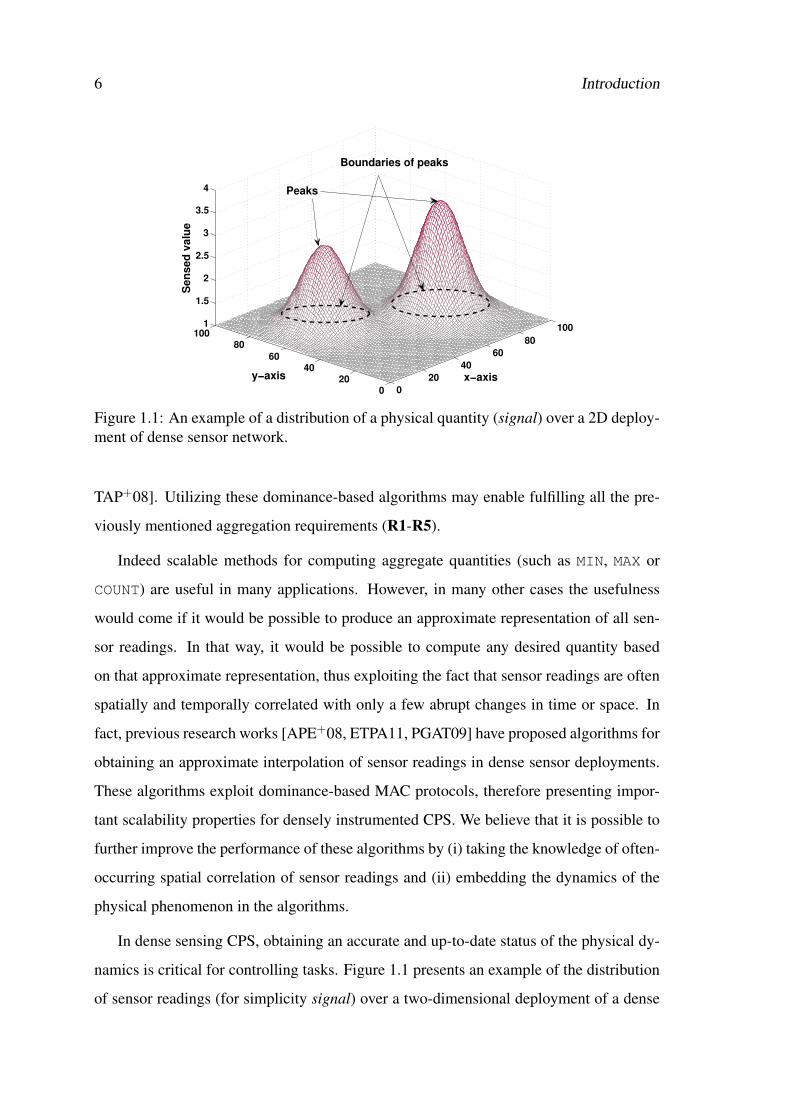
Figure 1.1: An example of a distribution of a physical quantity (signal) over a 2D deploy-ment of dense sensor network.
TAP+08]. Utilizing these dominance-based algorithms may enable fulfilling all the pre-
viously mentioned aggregation requirements (R1-R5).
Indeed scalable methods for computing aggregate quantities (such as MIN, MAX or
COUNT) are useful in many applications. However, in many other cases the usefulness
would come if it would be possible to produce an approximate representation of all sen-
sor readings. In that way, it would be possible to compute any desired quantity based
on that approximate representation, thus exploiting the fact that sensor readings are often
spatially and temporally correlated with only a few abrupt changes in time or space. In
fact, previous research works [APE+08, ETPA11, PGAT09] have proposed algorithms for
obtaining an approximate interpolation of sensor readings in dense sensor deployments.
These algorithms exploit dominance-based MAC protocols, therefore presenting impor-
tant scalability properties for densely instrumented CPS. We believe that it is possible to
further improve the performance of these algorithms by (i) taking the knowledge of often-
occurring spatial correlation of sensor readings and (ii) embedding the dynamics of the
physical phenomenon in the algorithms.
In dense sensing CPS, obtaining an accurate and up-to-date status of the physical dy-
namics is critical for controlling tasks. Figure 1.1 presents an example of the distribution
of sensor readings (for simplicity signal) over a two-dimensional deployment of a dense

1.3 Thesis Hypothesis 7
sensor network. Each data point in the signal represents a value measured by a sensor
node. Extracting features of the signal distribution, such as peaks and boundaries, is very
challenging in terms of timeliness and scalability. The main concern is to collect a subset
of readings with the most constructive information in a timely way. For instance, for very
dynamic signals (like pressure in air flow control application), there must exist a function-
ality that detects the rate of change in the dynamics of the signal and embed the change
into the algorithm. Dominance-based MAC protocols offer the potential to efficiently
compute simple aggregate quantities (MIN, MAX). These protocols require an interference
free medium for data transmission. However, this cannot be a valid assumption for wire-
less case.
We address the following challenges in this Thesis:
– How to devise a reliable data transmission for slotted WiDOM protocol that con-
siders a more realistic channel model that encompass interference.
– How to devise efficient aggregation algorithms that self adapt according to the
dynamics of the physical quantity and thus mitigating the accuracy problem (see
Chapter 3) of previously proposed algorithms.
– How to extract more sophisticated features (such as peaks or boundaries) also in a
scalable and efficient way.
1.3 Thesis Hypothesis
Consider a large-scale dense networked sensor system, whose nodes have a common sens-
ing goal: to measure a physical phenomenon and also to compute different features from
the distribution of sensor readings in order to trigger a set of control commands for the
actuators in a timely manner. Based on the aforementioned reasoning and problem state-
ment, we formulate the hypothesis as follows:
We believe that it is possible to extract certain features of a physical phe-
nomenon (e.g., the location and the intensity of an event, and the area af-
fected by the event) in a dense sensor network, in a reliable and timely way,
8 Introduction
and with a time complexity that is essentially independent of the number of
sensor nodes.
1.4 Research Objectives and Approach
The primary objective of this Thesis is to devise technologies and methodologies that
enable extracting certain features of a physical phenomenon monitored by a dense sensing
network in a timely and reliable manner. To reach this primary objective, a set of scientific
and technical objectives have been identified.
The first objective is to devise an error recovery scheme for the slotted WiDOM pro-
tocol in a noisy wireless channel. This scheme should enable reliable data transmission
in harsh environments where sensor nodes are more prone to interference. Typically,
wireless sensor nodes operate in the 2.4 GHz Industrial, Scientific and Medical (ISM)
band, which is shared by IEEE 802.15.1 (Bluetooth) and the far more powerful IEEE
802.11b/WiFi. Moreover, most commodity wireless devices (e.g. baby monitors, walkie-
talkies, and microwave ovens) use the same 2.4 GHz ISM band. Since all these systems
coexist in the ISM wireless spectrum, providing an error recovery scheme is paramount.
The approach we will follow will exploit an error recovery scheme by implementing data
acknowledgment (Ack) in slotted WiDOM protocol. This approach is further explained
in Chapter 4.
The second objective is to devise an aggregation mechanism that captures the dynam-
ics of the physical quantities and self adapts according to the physical changes. This
mechanism allows obtaining an accurate interpolation for a dynamic physical quantity.
To do so, we design an add-on functionality for the existing interpolation algorithm that
provides a set of change pattern metrics and updates these metrics in real-time. Further
details on this approach is explained in Chapter 5.
The third objective is to devise algorithms to identify various features in a distribution
of a physical phenomenon. Feature extraction algorithms enable identifying the location
and the boundaries of events in dense sensing applications. To achieve this objective a
set of functions were used for extracting various features from a distribution of physical

1.5 Research Contributions 9
quantity. These functions take advantage of prioritized MAC design to compute MIN/MAX
and employ them as the main element for the feature extraction purpose. we will describe
this approach in Chapter 6.
1.5 Research Contributions
We outline the scientific and technological contributions of the Thesis in the next para-
graph.
In the course of the work that led to this Thesis, we designed, implemented and val-
idated a reliable data transmission mechanism for slotted WiDOM protocol. In that di-
rection, in an initial phase of the work, we evaluated the schedulability analysis of slotted
WiDOM [VA10]. We then further extended the initial schedulability analysis by consider-
ing the error recovery mechanism for the case where sensor nodes suffer from interference
in the wireless channel. We devised the Ack-enabled slotted WiDOM in the Nano-RK
operating system [ERR05] and evaluated this protocol in a noisy environment. The most
important results are compiled and published as [VTTA15];
Another important set of results concerns the design and implementation of an adap-
tive aggregation algorithm that detects variations in the dynamics of the physical quantity
in real-time [VTA13]. These dynamics are embedded into the interpolation mechanism
to compensate the errors in the approximated representation of the physical quantity. The
implementation details of this algorithm are provided in this Thesis in Chapter 5.
At last but not the least, we designed and implemented several feature extraction
mechanisms suitable for dense sensor deployments. In particular, three distinct functions
were proposed to provide the location of peaks and the boundaries around them in the
distribution of a physical quantity (signal) [VGAT14]. An extension of the feature extrac-
tion mechanism to multi-hop dense network was then proposed [VGA+15]. Two distinct
approaches were used: (i) a classical clustering technique that extracts centrally the fea-
tures of the corresponding cluster and then transmit the information to the destination;
and (ii) a new technique (ripple-based) that employs flooding to find MIN/MAX globally.
In the ripple-based approach the features are computed in the same way as in a single

10 Introduction
broadcast domain. We compared these two approaches and showed their performance in
various scenarios. The code for this implementation is also available on-line [Vah15].
1.6 Structure of the Thesis
The remainder of this Thesis is organized as follows. In Chapter 2 we provide the neces-
sary background on dominance-based MAC protocols. Timeliness aspects are discussed
and other real-time MAC protocols, and characteristics are briefly surveyed. In Chapter
3 we review previous relevant work that exploits dominance-based MAC protocols to ef-
ficiently compute aggregate quantities. We discuss relevant aggregate quantities such as
MIN (the basic building block used in all algorithms aiming for computation other aggre-
gation quantities) and the more complex one (that includes positioning information) and
main focus of our work: complex feature extraction.
Chapters 4, 5 and 6 describe the main contributions attained in this research work. In
Chapter 4, we detail a novel proposal to improve the reliability of slotted WiDOM under
noisy channel conditions. Besides describing the implementation of the error detection
mechanism, we propose a novel response-time formulation that enables computing the
upper-bound on message transmission delay for slotted WiDOM. In Chapter 5, we present
and discuss the results on a novel sophisticated adaptive method to compute approximate
interpolation in densely-deployed sensor systems. In this method we present an add-on
functionality that computes the change pattern metric of the physical signal in order to
provide more accurate approximate representation of the physical signal. In Chapter 6 we
propose a set of algorithms that identify the main features of a sensor reading distribu-
tion and extend the proposed functionality to a large multi-hop dense network in a fully
distributed manner by leveraging the inherent properties of the dominance-based MAC
protocols.
Finally, in Chapter 7, we conclude this Thesis by providing a summary of the research
contributions and an outline of potential research challenges that build on the current
results.

Chapter 2
Background and Related Work —
Binary/Countdown MAC Protocols
In this chapter, we provide relevant background information regarding the family of
medium access control protocols used as a basis throughout the research work described
in this Thesis. First, a brief introduction to binary/countdown MAC protocol is provided.
Then, the adaptation of that MAC protocol to the wireless case, dubbed WiDOM (wireless
dominance), is described and important related research efforts surveyed.
2.1 Introduction
Real-time computing systems are those systems in which correctness of the system de-
pends not only on the logical result of computation but also on the time at which the results
are produced [SSH99]. This implies that, unlike more traditional information and com-
munication systems, where there is a separation between correctness and performance, in
real-time computing systems correctness and performance are tightly interrelated. Only
a few decades ago, real-time computing systems were an important but narrow niche of
computer systems, consisting mainly of military systems, air traffic control and embed-
ded systems for manufacturing and process control. This association caused that real-time
systems problems did not attract widespread interest from the computer community.
11

12 Background and Related Work — Binary/Countdown MAC Protocols
Meanwhile, the emergence of large-scale distributed systems, enabled by advances
in networking technology, has broaden real-time concerns into a mainstream enterprise,
with clients in a wide variety of industries and academic disciplines. Terms such as
“Cooperating-Objects” [MM09], “Cyber-Physical Systems” or “Internet of Things” [AIM10,
Kop11, SGLW09, COM09] have come to describe the research and technological efforts
that will ultimately efficiently allow interlinking the real world physical objects and cy-
berspace.
The integration of physical processes and computing is however nothing dramatically
new: embedded systems have been in place since a long time to denote systems that
combine physical processes with computing. The revolution is coming from extensively
networking embedded computing devices, in a blend that involves sensing, actuation,
computation, networking, pervasiveness and physical processes. And interaction with
the physical world always implies timeliness as a main concern in the design process.
This tendency has been establishing real-time technology as a priority for commercial
strategy and academic research for the foreseeable future and also for a wider number of
applications.
Collecting data from high-density networks can make use of specific properties of
the communication medium to collect aggregates in a fast and energy-efficient manner.
WiDOM [PAT07] is such a medium access control protocol that can be employed to ef-
ficiently compute aggregates in a timely manner with significantly lesser message ex-
changes, as shown in [PAT07, ETPA11]. With that approach, the number of messages
exchanged and time to gather an aggregate are not dependent on the number of nodes
in a given broadcast domain, thus facilitating dense networks without correspondingly
high-energy and temporal costs.
Acquiring the representation of the physical world must be done with a low (and
bounded) delay. Due to the large number of devices, which potentially offers high spatial
resolution, communication becomes challenging, and obtaining a representation of the
physical world with a low (and bounded) delay can be a major obstacle. So, the desire for
high spatial resolution may come at the cost of precluding high temporal resolution.
In [SAL+03] the authors outline various challenges in real-time communication in
2.2 Binary/Countdown MAC Protocols 13
sensor networks. Quality-of-Service oriented approaches, like those described in [FLE06],
provide probabilistic timing and reliability guarantees based on the application require-
ments. Such provisions are necessary in systems with real-time requirements, and espe-
cially in critical systems employed in for example, aeronautical applications. Reducing
the radio power can help not only to achieve energy-savings, but can also limit the radio-
coverage in dense networks, thereby reducing packet collisions. Low-power radio de-
signs [SAL+03, FLE06] have been proposed that can help on achieving the above goals.
Another approach to reduce the delay induced by wireless communication is the adop-
tion of decentralized computation. The analysis of sensor data within a small cluster of
nodes or locally on single nodes with the objective of extracting data features relevant for
the application will contribute to the reduction of the communication traffic. However,
it must be ensured that the energy and time saved on the communication is not lost with
the additional processing. The computation capabilities of the node must be then adapted
accordingly, using for example reconfigurable computing [HZG09].
2.2 Binary/Countdown MAC Protocols
Many emerging embedded applications are designed to respond to stimuli from the en-
vironment. Typically, these events are triggered sporadically; that is, the exact time of
a transmission request is unknown but a lower bound on the time between two consecu-
tive transmission requests from the same message stream is known. Such traffic is called
sporadic message streams.
While many scheduling algorithms and analysis techniques for wireless communica-
tions are available for periodic messages, the case of sporadic messages is less studied.
Most of the current wireless protocols cannot be analyzed to offer pre-run-time guaran-
tees that sporadic messages meet deadlines, and the protocols that do offer such guaran-
tees rely on polling, which is inefficient when the deadline is short and the minimum time
between two consecutive requests is long.
In wired networks, sporadic messages can be efficiently scheduled using the con-
troller area network (CAN) bus [Bos91], and this has already proven to be useful in
14 Background and Related Work — Binary/Countdown MAC Protocols
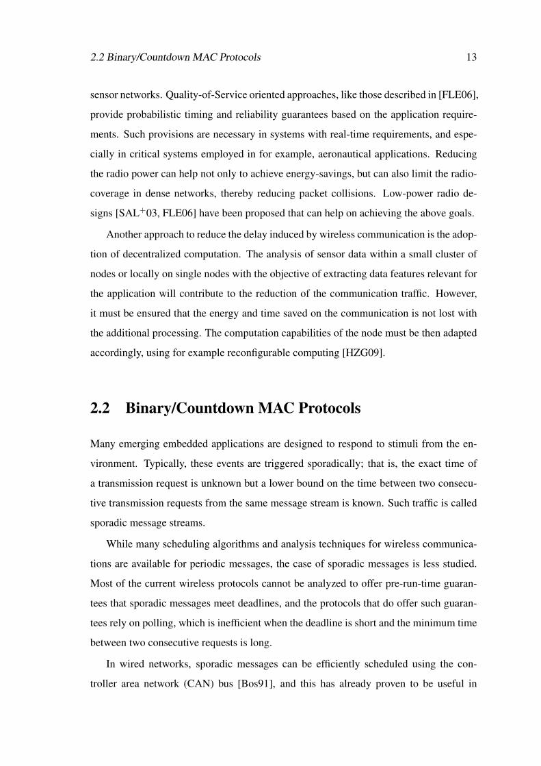
Figure 2.1: Arbitration in dominance/binary-countdown protocols.
industry, as witnessed by the pervasive use of the CAN bus. It has a medium access
control (MAC) protocol which is collision-free and prioritized, and hence it is possible to
schedule the bus such that if message characteristics (minimum inter-arrival times, trans-
mission times, jitter, etc.) are known, then it is possible to compute upper-bounds on
message delays [BLDB06, THW94].
This MAC protocol belongs to a family called dominance or binary countdown pro-
tocols [MW79]. In such protocols, messages are assigned unique priorities, and before
nodes try to transmit, they perform a contention resolution phase named arbitration such
that the node trying to transmit the highest-priority message succeeds.
During the arbitration (depicted in Figure 2.1), each node sends the message priority,
bit-by-bit, starting with the most significant one, while simultaneously monitoring the
medium. The medium must be devised in such a way that nodes will only detect a “1”
value if no other node is transmitting a “0”. Otherwise, every node detects a “0” value
regardless of what the node itself is sending. For this reason, a “0” is said to be a dominant
bit, while a “1” is said to be a recessive bit. Therefore, low numbers in the priority field
of a message represent high priorities.
If a node contends with a recessive bit but hears a dominant bit, then it will refrain

2.2 Binary/Countdown MAC Protocols 15
from transmitting any further bits, and will proceed only monitoring the medium. Finally,
exactly one node reaches the end of the arbitration phase, and this node (the winning node)
proceeds with transmitting the data part of the message. As a result of the contention for
the medium, all participating nodes will have knowledge of the winner’s priority.
Besides its ability to handle efficiently sporadic message streams, binary/countdown
MAC protocols can also be efficiently exploited to compute aggregate quantities. The
following example illustrates this.
The problem of obtaining aggregated quantities (e.g., MIN) in a single broadcast do-
main can be solved with a naive algorithm: every node broadcasts its sensor reading
sequentially. Hence, all nodes know all sensor readings and then they can obtain the ag-
gregated quantity. This has the drawback that in a broadcast domain with m nodes, at least
m broadcasts are required to be performed. Considering a network designed for m≥ 100,
the naive approach can be inefficient; it causes a large delay.
Let us consider the simple application scenario as depicted in Figure 2.2 (a), where a
node (node N1) needs to know the minimum (MIN) temperature reading among its neigh-
bors. Let us assume that no other node attempts to access the medium before this node.
A naive approach would imply that N1 broadcasts a request to all its neighbors and then
N1 would wait for the corresponding replies from all of them.
As a simplification, assume that nodes orderly access the medium in a time division
multiple access (TDMA) fashion, and that the initiator node knows the number of neigh-
bor nodes. Then, N1 can derive a waiting timeout for replies based on this knowledge.
Clearly, with this approach, the execution time depends on the number of neighbor nodes
(m).
Figure 2.2 (c) depicts another naive approach, but using a CAN-like MAC protocol.
Assume, in that case, that the priorities the nodes use to access the medium are ordered
according to the nodes’ ID, and are statically defined prior to runtime. Note that in order
to send a message, nodes have to perform arbitration before accessing the medium. When
a node wins, it sends its response and stops trying to access the medium. It is clear
that using a naive approach with CAN brings no timing advantages as compared to the
previous naive solution (Figure 2.2 (a)).

16 Background and Related Work — Binary/Countdown MAC Protocols
(a) Naïve algorithm (TDMA-like MAC) (b) Novel algorithm (CAN-like MAC)
(c) Naïve algorithm (CAN-like MAC)
Figure 2.2: Dominance/Binary-countdown arbitration motivating examples. (a) Exampleapplication with TDMA-like MAC; (b) possible solution by exploiting the properties of aCAN-like MAC, where priorities are assigned at runtime according to the sensed values;(c) possible solution using a CAN-like MAC with fixed priorities for the messages.
With such an approach, to obtain the minimum temperature among its neighbors, node
N1 needs to perform a broadcast request that will trigger all its neighbors to contend for
the medium using the prioritized MAC protocol. If neighbors access the medium using
the value of their temperature reading as the priority, the priority winning the contention
for the medium will be the minimum temperature reading.
With this scheme, more than one node can win the contention for the medium. But,
considering that at the end of the arbitration the priority of the winner is known to all
nodes, no more information needs to be transmitted by the winning node. In this scenario,
the time to obtain the minimum temperature reading only depends on the time to perform

2.3 Binary/Countdown MAC Protocols in Wireless 17
the contention for the medium, not on m. If, for example, one wishes that the winning
node transmits information (such as its location) in the data packet, then one can code the
priority of the nodes by adding a unique number (for example, the node ID) in the least
significant bits, such that priorities will be unique. Such use, results in a time complexity
of log m.
A similar approach can be used to obtain the maximum (MAX) temperature reading. In
that case, instead of directly coding the priority with the temperature reading, nodes will
use the bitwise negation of the temperature reading as the priority. Upon completion of
the medium access contention, given the winning priority, nodes perform bitwise negation
again to know the maximum temperature value.
MIN and MAX are just two simple and pretty much obvious examples of how aggregate
quantities can be obtained with a minimum message complexity (and therefore time com-
plexity) by exploiting binary/countdown MAC protocols, provided that message priorities
are dynamically assigned at runtime upon the values of the sensed quantity.
2.3 Binary/Countdown MAC Protocols in Wireless
WiDOM was proposed [PAT07] to solve the problem of sporadic messages scheduled on
a wireless channel, and it relies on adapting dominance/binary countdown protocols to
the wireless channel.
This adaptation is non-trivial due to the following reasons: (i) implementations of
dominance protocols for a wired medium are based on a wired-AND behavior of the
bus, where the dominant signal overwrites the recessive signal; (ii) these implementations
require that nodes are able to monitor the medium while transmitting—clearly this does
not easily extend to the case of wireless channels— and (iii) due to non-idealistic of the
used transceivers and nature of the wireless medium. In the following we explain the way
WiDOM overcomes all the mentioned issues.
WiDOM is composed of three phases: synchronization; contention resolution or tour-
nament; and data exchange —see Figure 2.3. In all dominance/binary countdown pro-
tocols, nodes need to agree on a common time before starting the contention resolution

18 Background and Related Work — Binary/Countdown MAC Protocols
… F E H G H H G ETG Tx/ Rx
(npriobit )
Synchronizat ion
phase
Tournament
phase
Data exchange
phase
Tim e
Ci”
Ci
Ci’
Figure 2.3: Timing order of the WiDOM protocol.
phase. This phase is of paramount importance since a small time drift in transmitting the
priority bits may lead to an erroneous result. Hence, the synchronization is needed to
provide a common reference point in time so that all nodes can start the competition at
the same time and it should happen right before the tournament phase.
In the initial version of WiDOM, at the start of synchronization, nodes should wait for
a long period of idle time “F” —see Figure 2.3, such that no node disrupts an ongoing
tournament. Then nodes with a pending message wait for another time span “E” to com-
pensate for the potential clock drift and also ensuring that all nodes have enough time to
listen for “F” time units. Afterwards, nodes start sending a carrier pulse for a duration of
“H” time units that signals the start of a tournament and establishes a common time refer-
ence. To do so, they have to switch from receive mode to send mode, which takes “SWX”
units of time. By sending this signal, all nodes restart their timers and synchronization
ends.
In the tournament phase, nodes transmit the priority of the message contending for the
medium bit-by-bit. If a node loses the contention of a bit (i.e. it transmits a recessive bit
and receives a dominant bit), it does not continue further bits and only proceed listening
to the medium to find out the priority of the winner. If a node does not lose the contention
during the current bit, it will proceed with the contention for the next bit.
The nodes that have a dominant bit, start transmitting a pulse of carrier for the duration
of “H” units of time, while nodes with a recessive bit perform carrier sensing for the same
time span. Also, note that the fact that wireless transceivers are not able to send and
receive simultaneously poses no problem to WiDOM since when a node has a dominant
2.4 Slotted WiDOM 19
bit, there is no need for reception and when a node has a recessive bit, it sends nothing; it
performs carrier sensing.
There is also a guarding time interval “G” to separate pulses of carrier waves. This
guarding time interval makes the protocol robust against clock inaccuracies, and takes
into account that signals need a non-zero time to propagate from one node to another. At
the end of the tournament, the node that does not receive a pulse wins the competition and
waits for “ETG” time units before starting data transmission.
2.4 Slotted WiDOM
The original implementation of WiDOM, explained in the previous section, is based on
commercial off-the-shelf (COTS) wireless sensor network (WSN) platforms. That ver-
sion of WiDOM implies a significant additional overhead. Part of that overhead is due
to technological limitations, importantly the switching time between transmission and re-
ception mode, that can be alleviated by carefully chosen hardware. Another part of that
overhead is caused by the required synchronization in which nodes should wait for a long
period of silence before any data transmission.
Slotted WiDOM is a more recent version of WiDOM aimed at reducing the overhead.
To do so, the authors have developed an add-on platform (called WiFLEX [PGAT09,
Gom08]) to perform the tournament phase more efficiently (lower overhead) and with
lower energy consumption. A novel synchronization mechanism that exploits an out-of-
band signaling technique was introduced in the design.
Most WSN platforms use the Chipcon CC2420 radio [T. 07], which does not offer the
desirable characteristics needed for the WiDOM implementation. In terms of hardware,
the WiFLEX approach consists of two small boards: the WiFLEX-main board (simply
main board), illustrated in Figure 2.4-(a), and the WiFLEX-daughter board (daughter
board), illustrated in Figure 2.4-(b). This platform can be plugged into common WSN
platforms such as the MicaZ [I. 04] or FireFly [MRR07]—see Figure 2.4.
The main board sends and receives pulses during the tournament, while the daughter
board, which is also known as WiFLEX-rxsync, is only responsible for receiving syn-

20 Background and Related Work — Binary/Countdown MAC Protocols
(c) WiFLEX_daughter board stacked
on the WiFLEX_main board
(d) WiFLEX platform stacked on
Firefly sensor
(e) WiFLEX platform stacked on
MicaZ sensor
(a) WiFLEX_main board
(b) WiFLEX_daughter board
Figure 2.4: Hardware platform.
chronization pulses. Figure 2.4-(c) shows how these two boards are assembled. The main
board is equipped with a low-power Micro-Controller Unit (MCU) in order to run the
MAC protocol on both the WiFLEX and the host platforms concurrently, and to provide
a mechanism for higher level communication between those two platforms. The MCU
controls two independent radio modules embedded in the main board: (i) one transmitter
and (ii) one receiver that share a single antenna. This antenna is assigned to each radio
module through a high-frequency switch under the MCU supervision.
Another single receiver module has been used in the daughter board that is always
ready to receive the synchronization signal. The advantage of using the separate receiver
(daughter board) is the possibility of setting it perpetually in reception mode and eliminat-
ing the switch time and maintaining accurate synchronization. Furthermore, by utilizing
out-of-band signaling for synchronization, nodes are not forced to wait for a long duration
of “F” time units. This allows a major reduction of the protocol overhead.
Poor balanced data (large number of consecutive 1’s or 0’s) results in unreliable sig-
nal detection on the receivers. To avoid this problem it is best to use data that has equal
number of 1’s and 0’s in a period of time. To provide such a balanced data on the receiver
2.4 Slotted WiDOM 21
Tx I dle Tx I dle Rx I dle Tx I dle
Dom inant bit
Bit stuffing
Recessive bit
Bit stuffing
1
0
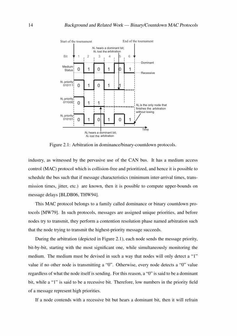
Figure 2.5: Dominant and recessive signal sequence with bit stuffing.
of the main board, a bit stuffing technique is exploited during the tournament phase. The
idea behind this technique is to introduce redundant information to maintain channel ac-
tivity. To do so, a dominant bit is coded as a “1” + “0” signal sequence and a recessive bit
as two consecutive “0” bits and then introducing a bit stuffing composed of a “1” + “0”
signal sequence after each dominant or recessive bit. See Figure 2.5 for illustration of this
principle.
In the tournament phase the radio module on the main board exchanges the data only
during priority bit exchange and after that it stays idle until the next tournament phase.
Since the radio activity is not maintained, the same problem may occur in the detection
of the first priority bit. To solve this problem, a special start symbol or preamble has been
introduced at the beginning of the tournament phase. Two consecutive dominant bits are
sufficient to allow a correct detection between noise and the start of an incoming priority
bit without imposing high overhead.
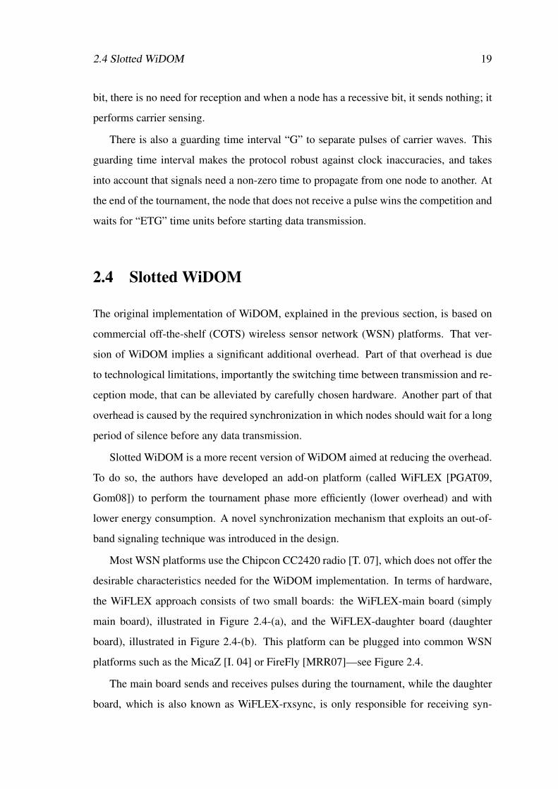
The same policy is also applied in the synchronization signal transmission. To main-
tain channel activity, a burst of consecutive sequence of “0” + “1” with the same pulse
duration is used. A longer duration of “1” pulse (for a duration of time for signal sens-
ing – TFSS) is then considered to signal the reception of a synchronization signal — see
Figure 2.6.
1
0
Tx
Idle
Tx
Idle
Tx
Idle
Tx
Idle
Idle
Tx
Tx Synch. Signal
TFSS
Start of synchronizat ion phase
End of synchronizat ion phase
Figure 2.6: Synchronization signal burst.

22 Background and Related Work — Binary/Countdown MAC Protocols
… TFSS A* B* H G H G H G H G ETG Tx/ Rx TFSS
Preamble (npriobit )x2
Synchronizat ion
phase
Tournament
phase
Data exchange
phase
Start of receiving
synch signal
Tim e
A*: (Prio_Tra); Transferring priority from WSN host platform to WiFLEX.
B*: (Win_Prio); Transferring winner priority from WiFLEX to WSN host platform.
Ci”
Ci
Ps
Figure 2.7: Timing order of the slotted WiDOM protocol.
This synchronization signal is broadcast periodically with a period of PS. Given the
periodic nature of such synchronization signal, which creates timeslots, we call this ver-
sion of WiDOM “slotted WiDOM”.
Summing up all the implementation details, the “superframe” of the Slotted WiDOM pro-
tocol is as depicted in Figure 2.7. There are three important issues that deal with the
add-on circuitry that is used in this implementation of WiDOM. These are outlined next.
(i) In the tournament phase, before going through the competition, the priority of the
enqueued message should be notified to the WiFLEX board and at the end of the
competition, the priority of the winner should be reported back to the WSN host
platform. Thus, in the slotted WiDOM , we need to consider two time intervals (A
and B) for internal communications between the two boards.
(ii) Only those nodes that have messages in their queues wait for receiving the synch
signal; this means that if a node enqueues a message slightly after the synch signal
broadcast, it will not participate in the currently on-going tournament, even if the
tournament phase formally has not started, yet.
(iii) Due to hardware shortcomings, bit stuffing is used after each priority bit and due
to the same reason two dominant bits instead of a single one should be sent as
preamble, to indicate the start of the contention period.

2.5 Other Prioritized Wireless MAC Protocols 23
Table 2.1: WiDOM parameters.
Parameter Description Implementation
PS Synchronization signal periodicity slotted WiDOMTFSS Time needed to sense synchronization signal slotted WiDOMA (PRIO_TRA) Priority transmission from WSN host to Wi-
FLEXslotted WiDOM
B (WIN_PRIO) Winner priority reported by WiFLEX slotted WiDOMH Carrier pulse duration BothG Guarding time Bothnpriobits Number of priority bits BothETG Guarding time at the end of tournament BothCi Time to transmit a message from message
stream i
Both
E Time to cope with synchronization imperfection WiDOMF Initial idle period for synchronization WiDOM
Table 2.1 summarizes all the parameters and their meaning for the two versions of
WiDOM.
2.5 Other Prioritized Wireless MAC Protocols
Guaranteeing timely delivery of critical traffic is a major challenge in time critical ap-
plications. Many research works have focused on minimizing the energy consumption
of these hardly resource-constrained networks. However, the real-time support to high
priority traffic within such applications has started to be investigated only recently. Some
attempts to support time guarantees in conventional protocols by assigning priorities to
the network traffic are reported in [SZBG14, AC01, SK96].
The definition of the WLAN standard, IEEE 802.11 [CWKS97], stimulated the de-
velopment of many prioritized carrier sense multiple access (CSMA) schemes. Some of
these variants, [AC01, BCV01, JC99], propose to fine tune the parameters defined in the
standard in order to guarantee that deadlines are met for each traffic flow. Some others,
e.g., [TWTLB11], suggest to combine time division multiple access (TDMA) approaches
with a traffic scheduler. Nevertheless, unless some additional scheduling features, such
as those described in [WIA11], are used, these techniques suffer from two drawbacks:
(i) they do not fully achieve a priority-based scheduling, since it may happen that a high
24 Background and Related Work — Binary/Countdown MAC Protocols
priority message has to wait in the transmission queue for a lower priority message to be
sent; and (ii) collisions may still occur, as a result of using CSMA in the IEEE 802.11.
Both problems certainly lead to deadline misses in real-time applications.
Due to collisions, nodes may suffer from long access delays before being able to trans-
mit. A conventional method is to send jamming signals (called Black Bursts, BB) in order
to win access for the transmission of higher priority messages [SK96, SK99]. Same ap-
proach is employed in the HIPERLAN protocol [JMMR97]. In BB-based protocols, a
station with real-time traffic waits until a channel becomes idle for a PCF 1 Inter-Frame
Space (PIFS) period and then contends for the channel by transmission of jamming sig-
nals. The collision interval between two or more pulses of energy is measured in order to
resolve the contention. The longest jamming transmission wins the channel access. After
transmitting the BB signal, a node waits for an observation time to check if any node is
transmitting a longer BB. If the channel remains idle during this time, the node sends its
data frame. A recent work [SZBG14] proposed the use of BB signals to distinguish the
highest priority and critical control packets. The drawbacks of BB signals lie in (i) the in-
ability to cope with the hidden terminal problem, and (ii) the unreliability in the presence
of interference.
Strawman [ÖMV+12] is designed for duty-cycled low-power networks. A Straw-
man round starts by receiving a COLLISION REQUEST packet. The senders interpret
this packet as the beginning of a new round, and contend for the channel by sending a
COLLISION packet of random length. Similar to the BB-based approach, the receiver es-
timates the length of the longest COLLISION packet and broadcasts a DECISION packet
containing the longest measured length, implicitly informing the corresponding transmit-
ter that it is granted access to the channel. Employing DECISION packets helps to allevi-
ate the hidden terminal problem. However, emitting pulses of energy or dummy packets,
a station wastes considerable channel bandwidth and energy to send each outgoing frame.
Moreover, this overhead (the length of BB or COLLISION packet) will increase linearly
with the number of priority levels since the maximum length of the black burst is propor-
tional to the number of priority levels. Therefore, only a small number of priority levels
1Point Coordination Function

2.5 Other Prioritized Wireless MAC Protocols 25
can be supported.
Another technique [YV06], not based on IEEE 802.11, implements prioritization by
using two separate narrow band busy-tones to communicate that a node is backlogged
with a high-priority message. This technique has the drawback of requiring very spe-
cialized hardware, requiring extra bandwidth (for the narrow band signals). Also, it only
supports two priority levels.
MAC protocols have also been proposed from the real-time systems community with
the goal of meeting deadlines [ZKI10, SRS12, KOK14]. Some protocols use tables
(sometimes called TDMA templates) with explicit start times of message transmission.
These tables are created at run-time either in a distributed fashion [CBBS03] or centrally
by a leader [LSR04]. It is also conceivable to use a TDMA template designed before run-
time [KG93] and use it to schedule wireless traffic. However, all these time-table driven
approaches have the drawback of requiring that sporadic message streams are dealt with
using polling, which, as previously stated, is inefficient.
Another approach, Implicit-EDF [CZSB02], is based on the assumption that all nodes
know the traffic on the other nodes that compete for the medium, and all these nodes
execute the EDF scheduling algorithm. Unfortunately, this algorithm is based on the
assumption that a node knows the arrival time of messages on other nodes, and this implies
that polling must be used to deal with sporadic message streams.
The standard IEEE 802.15.4 [80206] provides a Guaranteed Time Slots (GTS) mech-
anism to allocate specific duration within a superframe for soft real-time traffic. The
IEEE 802.15.4e Working Group redesigned the existing IEEE 802.15.4 MAC standard to
support emerging needs of embedded industrial applications. The Deterministic and Syn-
chronous Multi-channel Extension (DSME) mechanism in IEEE 802.15.4e [80212] is
one of the main extensions that provides prioritized channel access by reserving specific
DSME guaranteed time slots for high priority traffic. Through the DSME prioritization
method, the high priority messages are not transmitted immediately after their generation.
Devices wait for dedicated slots to transmit the messages. Thus, whenever a high prior-
ity message is generated after the dedicated time slot is passed, the device must wait for
the next assigned slots, thus the standard do not allow to resolve the priority inversion

26 Background and Related Work — Binary/Countdown MAC Protocols
problem.
Several industrial standards such as WirelessHART [wir10], ISA-100.11a [ISA09]
and WIA-PA [WIA11] leverage IEEE 802.15.4 physical layer with a low rate of maxi-
mum 250 kbps and a low implementation complexity for resource-constrained devices.
They mainly utilize TDMA approaches to provide guaranteed access to the wireless
medium. An adaptive scheduling algorithm can effectively improve the timeliness sup-
port by means of delay optimization or mitigation [TLB12, LRY+12]. The standards also
adopt packet-level channel hopping to improve the reliability of individual wireless links
by combating external interference and multi-path fading.
ISA-100.11a, WirelessHART and WIA-PA provide a limited service differentiation in
MAC schemes. They support four traffic categories. High-priority packets are allowed to
access the medium prior to low-priority packets. Hence, all data flows should be allocated
into one of these four classes of traffic flow and then a polling-based mechanism resolves
the competition among these traffic levels.
Another work called GinMAC [SBR10] is proposed to deliver data in a timely manner.
This protocol encompasses three procedures: off-line network dimensioning, an exclu-
sive TDMA schedule and delay conform reliability control to support timeliness require-
ments. In the implementation of GinMAC the traffic patterns and channel characteristics
are known a-priori and all complex calculations including slot allocation is done offline.
Due to off-line dimensioning, the protocol has a more predictable performance. Although
GinMAC can support mission-critical data delivery, it has some limitations. For example,
the protocol is tailored for a control loop setting in which sensor data must be forwarded
to the sink, resulting in a convergecast traffic pattern. Some mission-critical applications,
such as battlefield tracking, may create different traffic patterns and thus cannot be sup-
ported by GinMAC. Furthermore, as GinMAC is a TDMA-based protocol with exclusive
slot usage, it is suitable for a dense albeit relatively small network. In order to remove
this scalability restriction, additional work is required.
In [WUT05], a MAC protocol based on a binary countdown was proposed. However,
the binary countdown arbitration was employed such that collisions can cause deadline
misses.

2.6 Summary 27
2.6 Summary
This chapter provided background material on medium access control protocols relevant
to the proposed research work. We briefly introduced the binary/countdown MAC pro-
tocol. The main advantages of this MAC design were defined in terms of (i) timeliness
support for event-triggered messages and (ii) simultaneous non-destructive transmission
of information in a single broadcast domain. These will be shown to be important charac-
teristics to be exploited for efficient distributed computations in densely deployed sensor
networks.
Both wired (CAN bus) and wireless (WiDOM) versions of this MAC design were
described, including an add-on hardware to eliminate the shortcoming of the original
WiDOM implementation: slotted WiDOM.
While the CAN bus implements error recovery schemes, no such mechanism have
been devised for the WiDOM protocol. That would be relevant given the error prone
nature of wireless channels. We will address this challenge in Chapter 4 and propose a
novel solution to the problem.

28 Background and Related Work — Binary/Countdown MAC Protocols
Chapter 3
Background and Related Work –
In-network Data Aggregation
One of the key purposes of sensor network deployments is to collect data from the phys-
ical environment in order to obtain the desired information about the status of the phe-
nomena of interest. Data aggregation is defined as the process of aggregating data from
multiple sensor nodes to eliminate the redundant transmission and therefore to prolong
network lifetime. In this chapter, we survey various techniques of data aggregation in
sensor networks. A special focus is then given to the use of dominance-based technolo-
gies for computing aggregate quantities.
3.1 Data Aggregation Techniques
Data aggregation is used either to fuse data from different sensors to eliminate redundant
transmissions [KEW02, WFS08] or to fuse data and apply signal processing for comput-
ing some properties such as MIN (MAX), AVERAGE or SUM [MSFC02].
Data aggregation techniques are tightly coupled with how data is gathered at the sen-
sor nodes (data-centric) as well as how packets are routed through the network (routing-
centric) [FRWZ07]. There are two well-known categories for packet forwarding in the
network: tree-based and cluster-based approaches.
29

30 Background and Related Work – In-network Data Aggregation
According to the tree-based approach [IGE+03, LRS02, XHE01], first there is the
need to construct a spanning tree that is rooted at the sink node. Upon receiving a request
from the sink, nodes start performing in-network aggregation along the aggregation tree
by proceeding level by level from their leaves to their root. So, if two or more messages
arrive to a given node, their aggregate can be easily computed. The main drawback of this
approach is that due to channel impairments, it is possible to lose an aggregated data. In
fact, a single message at a given level of the tree may aggregate the data coming from the
whole related sub-tree. When a packet is lost at a given level of the tree, the data coming
from the related sub-tree will be lost as well.
The cluster-based approaches [Hei00, MR04, YG02, ZNLF04] are also based on a
hierarchical organization of the network. Initially, nodes are subdivided into clusters and
a special node, called cluster-head, is selected in each cluster. The cluster-head nodes are
elected in order to aggregate data locally and transmit the result of such an aggregation to
the sink. If the sink node loses the packet coming from a cluster-head, it will lose all the
information about the underlying cluster.
Several studies have been done on real-time data aggregation. Most of these stud-
ies couple the aggregation mechanism with the underlying routing or MAC approaches.
Zhang et al. [ZJX10] investigated the problem of maximizing information collection un-
der a delay bound constraint for CSMA/CA-based MAC protocols in sensor networks.
They proposed an optimal algorithm and a distributed heuristic algorithm to allocate the
maximal allowable transmission delay at each sensor node. Although, their approach
does not guarantee the reception of all measurements; they have achieved the information
collection ratio of 95% in the best case.
A different approach to route packets by performing data aggregation is presented
in [DBMC04], where the routing and the MAC protocols are jointly designed. The pri-
mary objective of the Delay Bounded Medium Access Control (DB-MAC) [DBMC04]
scheme is to minimize the latency for delay bounded applications while taking advantage
of data aggregation mechanisms for increased energy efficiency.
However, considering a dense network, all the aforementioned protocols suffer from
poor timeliness. The time complexity of finding a simple aggregate quantity (e.g. MIN)

3.2 Boundary Detection Techniques 31
depends on either the number of nodes in the same broadcast domain, if a TDMA MAC
approach is used, or on the number of allowable retransmissions and some none deter-
ministic factors, if a contention-based MAC protocol is used.
3.2 Boundary Detection Techniques
Boundary detection in sensor networks often aimed in various applications. There are
different approaches to address the problem of boundary detection and determining the
extent of an event in sensor networks [CG03, NM03, WGM06, SBP04, ATS14].
Chintalapudi and Govindan presented localized edge detection techniques based on
statistics, image processing, and classification [CG03]. Nowak and Mitra described a
method for hierarchical boundary estimation using recursive dyadic partitioning [NM03].
They developed an inverse proportionality relation between energy consumption and the
mean-square error in boundary detection and showed that their method is near-optimal
with respect to this fundamental trade-off. Another hierarchical boundary estimation is
proposed in [ATS14], where a contiguous two-dimentional shape of an event is found
with a threshold-based boundary detection.
Other schemes represent the boundary of an event or the signal landscape of a sensor
network compactly using in-network aggregation [BGHS06, GSW09, HHMS03, DRK11,
HR10]. Gandhi et al. studied the problem of monitoring the events of sensor networks
using sparse sampling [GSW09]. However, their algorithm requires the prior knowledge
of the event geometry (e.g. circle, ellipse, or rectangle) for computational efficiency.
Similar method has been explored in [DRK11], which utilized a regression-based spatial
estimation technique to determine discrete points on the boundary. Ham et al. present
a distributed boundary detection based on in-network aggregation in which only sensor
nodes that identify a boundary transmit their observation to the remote station [HR10].
To that end, they first applied a Delaunay triangulation to determine the neighbors of
each node and then generate boundary segments between neighboring sensors. However,
this algorithm cannot be known as a fully decentralized approach since the two steps
mentioned above should be done centrally through a remote station.

32 Background and Related Work – In-network Data Aggregation
There are also contour-based methods for deciding the type of an event [XLCL06,
LL10]. In these works, the authors consider energy-efficient techniques to construct and
incrementally update a number of two-dimentional contour maps in a sensor network.
Another field of research involving detecting holes and topological features in a sensor
network is presented in [Fun05, KFPF06]. In these approaches, local connectivity graphs
are used to infer static features of an event but these approaches require the involvement
of all the nodes in the network.
3.3 Scalablity Issues
Most of the techniques mentioned in Sections 3.1 and 3.2 exploit the opportunities for par-
allel transmission and of en-route aggregation of data. However, in densely instrumented
systems where even a very small area may contain several hundreds of sensor nodes, the
performance of the common data aggregation techniques is limited by the fact that nodes
in the same broadcast domain cannot transmit in parallel. Thus, the time-complexity of
those approaches also heavily depends on the number of sensor nodes. This results in
long delays for collecting the information of all nodes and obtaining the required set of
measurements.
In this context, dominance-based protocols have emerged as an enabler protocol for
efficient aggregation techniques offering a much lower time complexity. The following
subsections describe in detail techniques that exploit dominance-based MAC protocols to
efficiently compute aggregate qualities with a time complexity that is independent of the
number of nodes in a broadcast domain. Basic aggregate quantities such as MIN will be
addressed, as well more complex ones such as approximate interpolation, which builds
on the MIN “primitive”.

3.4 Computing Aggregate Quantities by Exploiting Dominance 33
3.4 Computing Aggregate Quantities by Exploiting Dom-
inance
It is possible to devise algorithms for sensor data processing such that its time-complexity
is independent of the number of nodes. In fact, if each node uses the value of its sensor
reading instead of an arbitrary priority, the node winning the contention for the medium
will be the one with the minimum (MIN) of the sensed values [APE+08, ETPA11, PGAT09].
It is straight forward for the case where all measured values are non-negative. However,
for the case where negative values are involved, sensor nodes should add an offset to their
measurements before starting the arbitration, in order to be sure that all values are non-
negative. In [APE+08], it is demonstrated that CAN-enabled platforms can be used to
compute various aggregate quantities. In [PGAT09] the authors show the same, but using
slotted WiDOM.
In order to understand how a dominance-based MAC protocol can be used to effi-
ciently compute an aggregate quantity, consider a simple example of how to compute the
minimum of all sensor readings. One naïve approach as shown in Figure 2.2 (a) would
be to use a time-division multiple-access (TDMA) scheme and assign one timeslot to
each sensor node and let a sensor node transmit its sensor reading in its slot. After one
TDMA cycle, a node knows all sensor readings and the MIN value can be computed but,
unfortunately, the time-complexity is O(m), where m is the number of sensor nodes. The
same type of naïve scheme can be implemented with a prioritized MAC protocol. Fig-
ure 2.2 (c) shows this. Nodes contend with each other and each time the winner sends
its measured value to the sink and similarly the MIN value is computed. Now consider
a prioritized MAC protocol where a sensor node uses its sensed data as its priority. The
MAC protocol will grant medium access to the sensor node with the minimum sensor
reading —see Figure 2.2 (b). Since a dominance-based prioritized MAC protocol makes
all sensor nodes know the priority of the sensor node which was granted the medium, it
holds that all sensor nodes will know the minimum of the sensor reading. This makes it
possible to compute MIN.
The importance of the above method is that its time-complexity is independent of

34 Background and Related Work – In-network Data Aggregation
the number of nodes in the broadcast domain. Similarly, the maximum value (MAX) can
be obtained by this method. The only difference is that for computing the MAX value
nodes use the bitwise negation of their sensed values as their priorities and compete for
channel. The computation time of this method has a time complexity of O(npriobits),
where npriobits is the number of bits used to represent the data (priority).
Other aggregate quantities (even if approximations) such as COUNT, AVERAGE, and
SUM can be computed using same building block as explained in computing MIN and
MAX [APT09]. It is also possible to track how a physical quantity varies over an area ob-
served by a dense network with the time-complexity that does not depend on the number
of sensor nodes.
In our work we are particularly interested in how to perform sensing in a densely
deployed sensor network. Approximate interpolation is an approach we will exploit.
3.5 The Basic Interpolation Algorithm
Each node is assumed to be able to take sensor readings and to know its location. All
nodes use the same function to interpolate the sensor data. Nodes start with the inter-
polation function being a flat surface. Then, at each round, one node, which is called
control point, will be selected and broadcast its measured value together with its location.
Upon receiving the message, other nodes re-compute the interpolation function and this
procedure iterates for a predefined number of iterations (k). Since at each iteration one
control point is selected, k also represents the number of control points used to obtain an
interpolation.
In order to find the most effective subset of control points, the technique described
previously for finding the MIN value is used. In the Basic Interpolation Algorithm (BIA)
[APE+08], the node with the highest interpolation error has the highest priority to send
its value. For a node ni, the interpolation error ei is defined as the absolute difference of
its sensor value, vi, and its interpolated value, f (xi,yi):
ei = |vi− f (xi,yi)| (3.1)

3.5 The Basic Interpolation Algorithm 35
where xi and yi are space coordinates and the function f (x,y) approximates the sensor
readings throughout the area of interest. The next step is to provide an interpolation
function which is represented by a set of control points S. Each control point pi ∈ S has
three attributes: xi, yi and vi. The value of the approximate interpolation at the location
(xi,yi) is given by vi . In each iteration, the node with the highest interpolation error
is found and is added to the set of control points, S. The interpolation function f (x,y)
—also called weighted-average interpolation (WAI) function [SS04, She, TOMO05]— is
mathematically defined as follows:
f (x,y) =
0 if S = /0
vi ∃Pi ∈ S : xi = x∧ yi = y
Σi∈svi·wi(x,y)Σi∈swi(x,y)
otherwise
(3.2)
where wi(x,y) is a weight that is inversely proportional to the distance between the ith
control point and the point in the location (x,y), and is given by:
wi(x,y) =1
(xi− x)2 +(yi− y)2(3.3)
Algorithm 1 shows the pseudo code corresponding to BIA. It must be mentioned that
this procedure is executed by all nodes so that all of them have the same approximation of
the interpolation. This algorithm is valid for the case where we deal with a smooth phys-
ical signal that exhibits comparably (to the time the computation takes) slow variations
over time. It is also assumed that there are no faulty sensors in the network.
Algorithm 1: Basic Interpolation Algorithm
input : Number of iteration (k)output: Approximate interpolation of sensor readings
1 S← /02 for i = 1 : k do
3 re-compute the interpolation value according to Equation 3.24 calculate ei
5 select the sensor node ni with maximum ei
6 add the node ni to the set of control points S
7 end

36 Background and Related Work – In-network Data Aggregation
(a) Original Signal (b) Interpolated Signal
Figure 3.1: Interpolation example (taken from [APE+08]).
Figure 3.1 illustrates the operation of the BIA scheme for a given example. Fig-
ure 3.1 (a) shows how a physical quantity varies as a function of space coordinates x and
y. Figure 3.1 (b) shows an interpolation which is an approximate representation of this
physical quantity; the lines indicate the location of control points in the set S.
In the following sub-sections we discuss variations of the algorithm that address the
above mentioned shortcomings.
3.6 The Differential Interpolation Algorithm
BIA is good when the physical quantity changes very little during the execution of the in-
terpolation algorithm. There are applications that track a low changing phenomenon such
as temperature or humidity. However, this is not the case of some others such as active air
flow control in aircraft [TPB+12, LRT15]. Ignoring the dynamics of the physical quan-
tities causes the interpolation represented by the set of control points S to significantly
diverge from the real state of the physical quantity being monitored.
A possible solution to tackle this problem — the differential interpolation algorithm
(DIA) proposal [ETPA11]— is to embed the physical change pattern into the interpolation
algorithm. To do so, each time after adding a new control point to the set S (Line 6 in
Algorithm 1), the previous selected control points in S should be updated based on a
model that emulates the dynamics of the physical environment. The pseudo-code of the
updated algorithm is shown in Algorithm 2. An application designer must define the
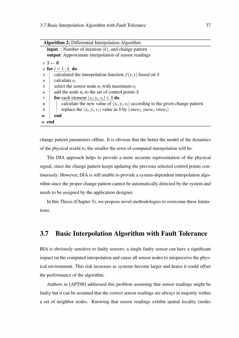
3.7 Basic Interpolation Algorithm with Fault Tolerance 37
Algorithm 2: Differential Interpolation Algorithm
input : Number of iteration (k), and change patternoutput: Approximate interpolation of sensor readings
1 S← /02 for i = 1 : k do
3 calculated the interpolation function f (x,y) based on S
4 calculate ei
5 select the sensor node ni with maximum ei
6 add the node ni to the set of control points S
7 for each element (xi,yi,vi) ∈ S do
8 calculate the new value of (xi,yi,vi) according to the given change pattern9 replace the (xi,yi,vi) value in S by (xnewi,ynewi,vnewi)
10 end
11 end
change pattern parameters offline. It is obvious that the better the model of the dynamics
of the physical world is, the smaller the error of computed interpolation will be.
The DIA approach helps to provide a more accurate representation of the physical
signal, since the change pattern keeps updating the previous selected control points con-
tinuously. However, DIA is still unable to provide a system-dependent interpolation algo-
rithm since the proper change pattern cannot be automatically detected by the system and
needs to be assigned by the application designer.
In this Thesis (Chapter 5), we propose novel methodologies to overcome these limita-
tions.
3.7 Basic Interpolation Algorithm with Fault Tolerance
BIA is obviously sensitive to faulty sensors; a single faulty sensor can have a significant
impact on the computed interpolation and cause all sensor nodes to misperceive the phys-
ical environment. This risk increases as systems become larger and hence it could offset
the performance of the algorithm.
Authors in [APT08] addressed this problem assuming that sensor readings might be
faulty but it can be assumed that the correct sensor readings are always in majority within
a set of neighbor nodes. Knowing that sensor readings exhibit spatial locality (nodes
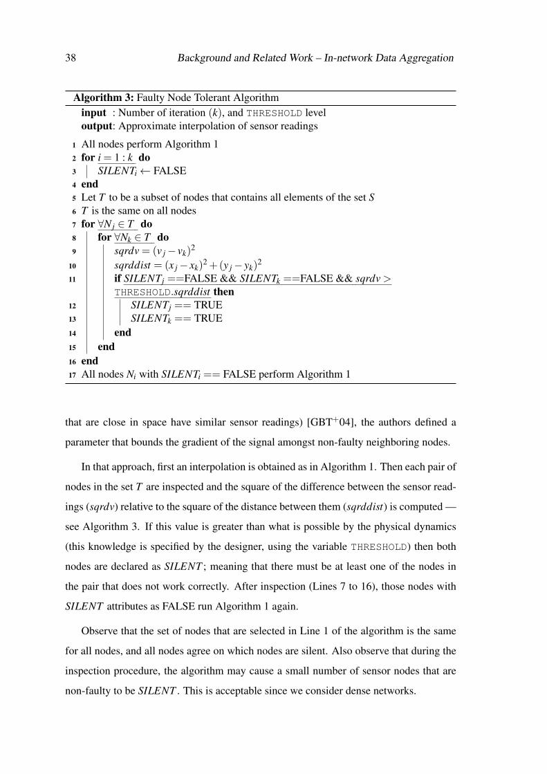
38 Background and Related Work – In-network Data Aggregation
Algorithm 3: Faulty Node Tolerant Algorithm
input : Number of iteration (k), and THRESHOLD leveloutput: Approximate interpolation of sensor readings
1 All nodes perform Algorithm 12 for i = 1 : k do
3 SILENTi← FALSE4 end
5 Let T to be a subset of nodes that contains all elements of the set S
6 T is the same on all nodes7 for ∀N j ∈ T do
8 for ∀Nk ∈ T do
9 sqrdv = (v j− vk)2
10 sqrddist = (x j− xk)2 +(y j− yk)
2
11 if SILENTj ==FALSE && SILENTk ==FALSE && sqrdv >THRESHOLD.sqrddist then
12 SILENTj == TRUE13 SILENTk == TRUE14 end
15 end
16 end
17 All nodes Ni with SILENTi == FALSE perform Algorithm 1
that are close in space have similar sensor readings) [GBT+04], the authors defined a
parameter that bounds the gradient of the signal amongst non-faulty neighboring nodes.
In that approach, first an interpolation is obtained as in Algorithm 1. Then each pair of
nodes in the set T are inspected and the square of the difference between the sensor read-
ings (sqrdv) relative to the square of the distance between them (sqrddist) is computed —
see Algorithm 3. If this value is greater than what is possible by the physical dynamics
(this knowledge is specified by the designer, using the variable THRESHOLD) then both
nodes are declared as SILENT ; meaning that there must be at least one of the nodes in
the pair that does not work correctly. After inspection (Lines 7 to 16), those nodes with
SILENT attributes as FALSE run Algorithm 1 again.
Observe that the set of nodes that are selected in Line 1 of the algorithm is the same
for all nodes, and all nodes agree on which nodes are silent. Also observe that during the
inspection procedure, the algorithm may cause a small number of sensor nodes that are
non-faulty to be SILENT . This is acceptable since we consider dense networks.
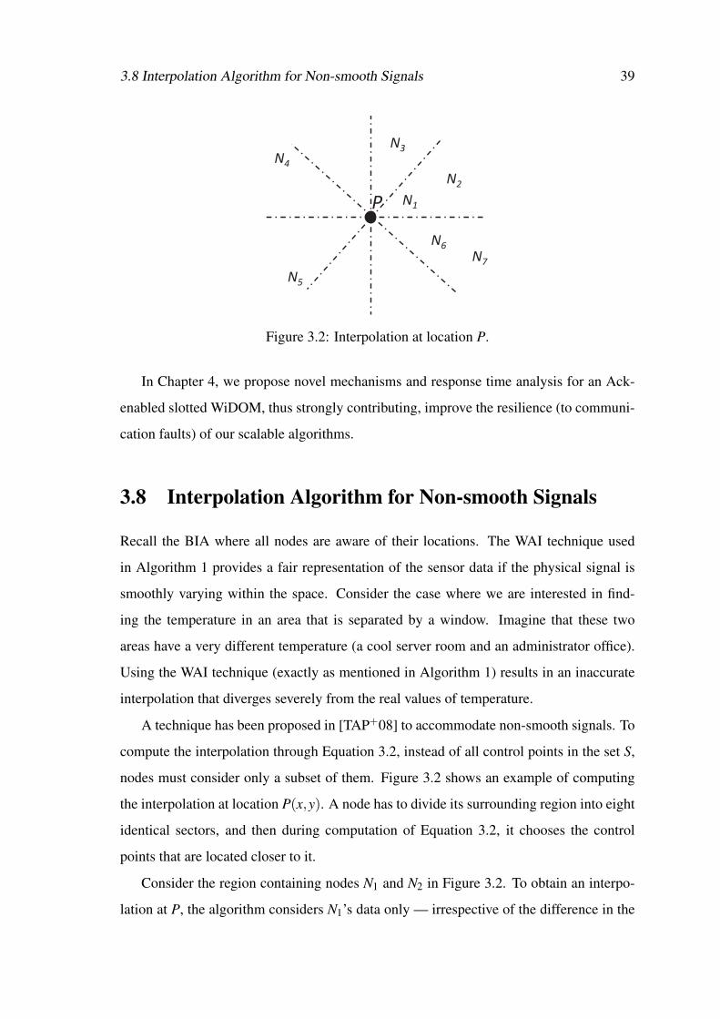
3.8 Interpolation Algorithm for Non-smooth Signals 39
P
N5
N4
N3
N1
N2
N7
N6
Figure 3.2: Interpolation at location P.
In Chapter 4, we propose novel mechanisms and response time analysis for an Ack-
enabled slotted WiDOM, thus strongly contributing, improve the resilience (to communi-
cation faults) of our scalable algorithms.
3.8 Interpolation Algorithm for Non-smooth Signals
Recall the BIA where all nodes are aware of their locations. The WAI technique used
in Algorithm 1 provides a fair representation of the sensor data if the physical signal is
smoothly varying within the space. Consider the case where we are interested in find-
ing the temperature in an area that is separated by a window. Imagine that these two
areas have a very different temperature (a cool server room and an administrator office).
Using the WAI technique (exactly as mentioned in Algorithm 1) results in an inaccurate
interpolation that diverges severely from the real values of temperature.
A technique has been proposed in [TAP+08] to accommodate non-smooth signals. To
compute the interpolation through Equation 3.2, instead of all control points in the set S,
nodes must consider only a subset of them. Figure 3.2 shows an example of computing
the interpolation at location P(x,y). A node has to divide its surrounding region into eight
identical sectors, and then during computation of Equation 3.2, it chooses the control
points that are located closer to it.
Consider the region containing nodes N1 and N2 in Figure 3.2. To obtain an interpo-
lation at P, the algorithm considers N1’s data only — irrespective of the difference in the
40 Background and Related Work – In-network Data Aggregation
data values at N1 and N2. Intuitively, if the difference is significant, for example due to
a wall in between the two nodes, then taking N2’s data into account will lead to interpo-
lation inaccuracy. In other words, N1’s data “masks” N2’s. Following this argument, the
nearest neighbor of P from each of the sectors constructs the subset T ⊂ S that is used to
compute interpolation. Therefore, in this example, T = (N1,N3,N4,N5,N6).
Although this method provides a viable solution for non-smooth signals, it increases
the time-complexity of the algorithm and only offer a fair interpolation if it runs for a
large number of iterations, which implies the use of a large number of control points.
3.9 Concluding Remarks
In this chapter, we surveyed previous relevant works on data aggregation and boundary
detection. We showed that the related works are unable to efficiently satisfy the real-time
requirements considering the nature of dense sensing systems. We stressed the importance
of dominance-based MAC protocols to support aggregate quantity computations in such
dense sensed environments.
We reviewed relevant work that has been exploiting dominance-based approach. We
identified some limitations in those works, for which we propose solutions in Chapters 4,
5 and 6 of this Thesis

Chapter 4
Improving the Reliability of Slotted
WiDOM
In this chapter, we focus on a new version of WiDOM (dubbed slotted WiDOM), which
offers lower overhead as compared to the original version, and propose a new schedula-
bility analysis for slotted WiDOM that considers message streams with release jitter. In
order to provide a timing analysis with higher practical value, the effect of transmission
faults must be taken into account. Therefore, in our novel analysis, we consider the case
where messages are transmitted in more realistic wireless channels affected by noise and
interference.
4.1 Introduction
In order to guarantee the timeliness of a message stream, there must exist a pre-run-time
analysis to show whether it is feasible to accommodate this set of message streams such
that no messages miss their deadlines. Indeed, the design of a real-time and reliable
wireless MAC protocol that is able to efficiently handle event-driven (sporadic) messages
needs the following requirements to be met:
R1 A prioritized MAC protocol should exist for a wireless channel. Among all com-
puter nodes that request to transmit, this protocol grants the right to transmit on the
channel to the computer node with the highest priority message;
41

42 Improving the Reliability of Slotted WiDOM
R2 The overhead related to the arbitration of the prioritized MAC protocol should scale
(grow slowly) with the number of priority levels;
R3 A schedulability analysis should exist for the prioritized MAC protocol;
R4 The schedulablity analysis should take into consideration the case where corrupted
messages in a noisy channel impose the need for retransmission.
Finally, in order to obtain an efficient system, the following requirement should also be
satisfied:
R5 The overhead related to the arbitration of the prioritized MAC protocol should be low.
Unfortunately, the current state of the art cannot fulfill all these requirements. The
Controller Area Network (CAN) [Bos91], which is devised for a wired channel, offers
many priority levels (hence fulfilling R2). For the wireless version of CAN, dubbed
WiDOM [PAT07, AT06], there exists a corresponding schedulability analysis as well
(hence fulfilling R1, R2 and R3), but the existing analysis is based on the assumption
that no errors can happen during the message transmission (missing R4). Another prob-
lem with this protocol is that it imposes a large overhead (missing R5). On this account,
the slotted WiDOM [13], already mentioned in Chapter 2, offers low overhead (hence
fulfilling R1, R2 and R5) but no schedulability analysis is available for it. The develop-
ment of a schedulability analysis for slotted WiDOM — with the capability of analyzing
the responsiveness of message streams that suffer from release jitter and also experience
noise on the channel — would, however, offer us the missing piece in fulfilling the five
requirements listed above.
In this chapter, we also introduce a technique for error recovery in the slotted WiDOM
such that the protocol is made more reliable under poor channel conditions. We develop a
novel schedulability analysis for slotted WiDOM taking into account the erroneous trans-
missions of messages which may happen under noisy conditions. Previous work [PAT07]
has already provided the schedulability analysis of WiDOM, but that analysis is only ap-
plicable to the basic implementation, not to the slotted version. It also considers that all
messages are transmitted over an error-free channel.

4.2 Ack-Enabled Slotted WiDOM 43
In the following sections, we first explain the error recovery mechanism proposed
for the slotted WiDOM and then we present a new schedulability analysis that takes into
account the erroneous transmissions of message.
4.2 Ack-Enabled Slotted WiDOM
Besides physical aspects related to signal propagation, in a wireless channel a commu-
nication error may result from the interference due to various transmitters sharing the
same frequency band, like Wi-Fi, Bluetooth and other sensor networks. It may also come
from the presence, in the vicinity, of electromagnetic sources such as electric motors or
microwave ovens.
To minimize the impact of external interferers on the reliability of the system, we im-
plement an error recovery scheme based on acknowledgment (Ack) packet transmission
after receiving any data packet. Through this scheme, if the sender does not receive back
an Ack packet from the receiver during a predefined period of time, it will re-issue the
data transmission. In other words, the sender retries to send the same packet in the next
tournament and retransmit the data until it receives the Ack from the intended receiver.
It should be mentioned that the retransmission of the corrupted packet may not happen
immediately after the erroneous transmission, since a higher priority message may be
enqueued while the sender is waiting for the Ack of the previous transmission.
Note that the error recovery method that we use for WiDOM is not exactly similar to
the one that is used in the CAN bus. Unlike CAN, we do not need to globalize a detected
error because in this version of WiDOM we are dealing with unicast transmissions, not
multicast. To save more resources, we do not assign an individual timeslot for sending the
Ack packet, since the Ack packet size is comparatively smaller than the data packet size
and can be transmitted at the end of data transmission within the same timeslot. Figure 4.1
shows the “superframe” of the slotted WiDOM protocol. The ACK box in the figure is
considered to accommodate the switching time (from send mode to the receive mode) and
also the time duration a node needs to wait to receive the Ack message from the receiver.
Accordingly, the periodicity of PS should be chosen in a way that a message with the
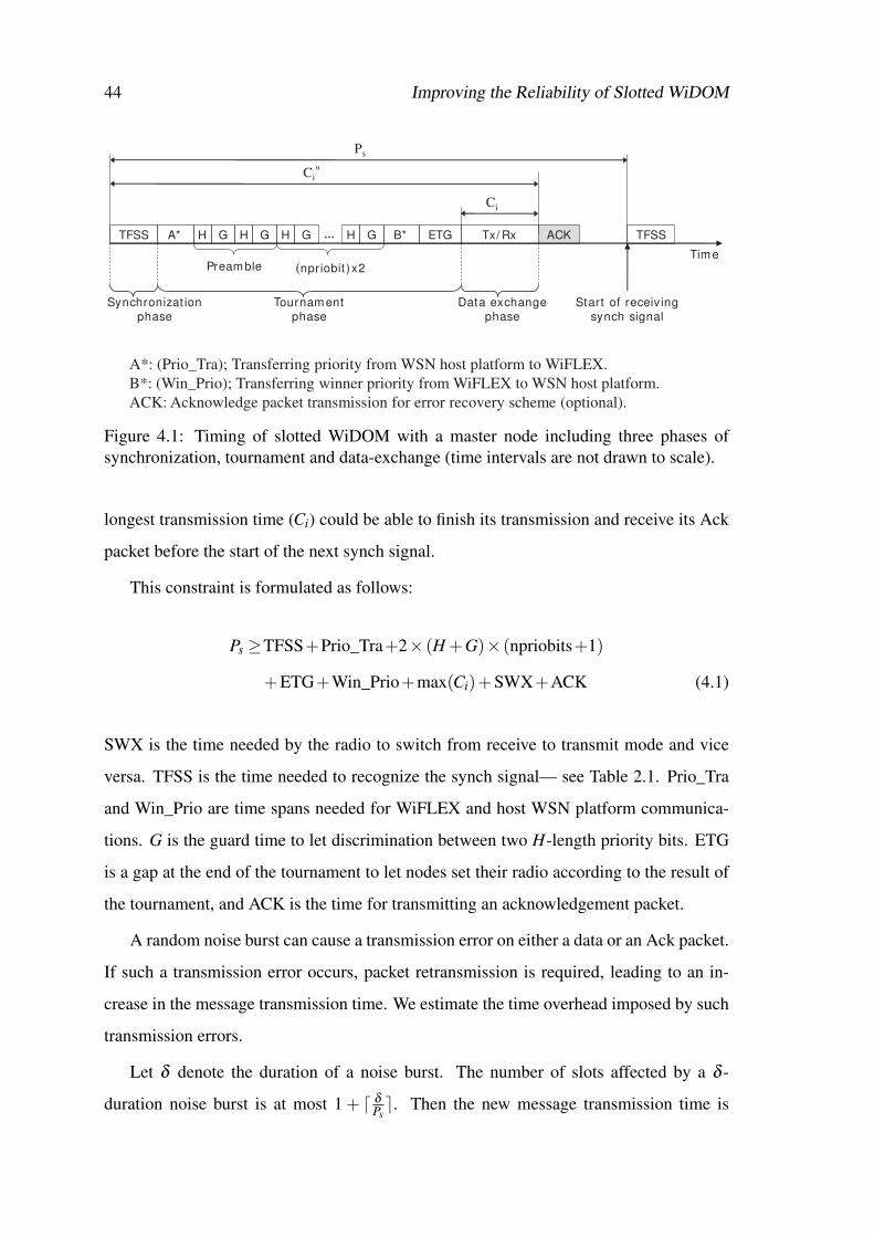
44 Improving the Reliability of Slotted WiDOM
… TFSS A* B* H G H G H G H G ETG Tx/ Rx ACK TFSS
Preamble (npriobit )x2
Synchronizat ion
phase
Tournament
phase
Data exchange
phase
Start of receiving
synch signal
Tim e
A*: (Prio_Tra); Transferring priority from WSN host platform to WiFLEX.
B*: (Win_Prio); Transferring winner priority from WiFLEX to WSN host platform.
ACK: Acknowledge packet transmission for error recovery scheme (optional).
Ci”
Ci
Ps
Figure 4.1: Timing of slotted WiDOM with a master node including three phases ofsynchronization, tournament and data-exchange (time intervals are not drawn to scale).
longest transmission time (Ci) could be able to finish its transmission and receive its Ack
packet before the start of the next synch signal.
This constraint is formulated as follows:
Ps ≥TFSS+Prio_Tra+2× (H +G)× (npriobits+1)
+ETG+Win_Prio+max(Ci)+SWX+ACK (4.1)
SWX is the time needed by the radio to switch from receive to transmit mode and vice
versa. TFSS is the time needed to recognize the synch signal— see Table 2.1. Prio_Tra
and Win_Prio are time spans needed for WiFLEX and host WSN platform communica-
tions. G is the guard time to let discrimination between two H-length priority bits. ETG
is a gap at the end of the tournament to let nodes set their radio according to the result of
the tournament, and ACK is the time for transmitting an acknowledgement packet.
A random noise burst can cause a transmission error on either a data or an Ack packet.
If such a transmission error occurs, packet retransmission is required, leading to an in-
crease in the message transmission time. We estimate the time overhead imposed by such
transmission errors.
Let δ denote the duration of a noise burst. The number of slots affected by a δ -
duration noise burst is at most 1 + ⌈ δPs⌉. Then the new message transmission time is

4.2 Ack-Enabled Slotted WiDOM 45
TFSS
Time
Tournament Tx/Rx ACK TFSS Tx/Rx ACK
Ps Ps
Noise burst
Noise burst
Tournament
Figure 4.2: Error caused by a noise burst with length of one timeslot.
delayed by (D(δ )), computed as follows:
D(δ ) = Ps×(
1+
⌈
δ
Ps
⌉)
. (4.2)
Figure 4.2 shows an example of a noise burst with duration of one timeslot (δ = Ps)
that can add a delay of up to 2Ps on the message transmission time.
Given F(∆t), an error function modeling the interference in a wireless channel during
an interval ∆t, the maximum incremental delay due to the error recovery scheme is:
E(∆t) = D(δ )×F(∆t). (4.3)
Similarly to the technique proposed by the authors in [BVN+11], we consider two
different types of noise sources: (i) a periodic noise burst with the period of Tp and the
burst duration of δp; and (ii) a sporadic noise burst with a minimum inter-arrival time of Ts
and a burst duration of δs. The sporadic noise models the interference caused by packet-
based radios (e.g., Wi-Fi, Bluetooth) while the periodic noise models the interference
induced by other electromagnetic noise sources. So, being K the number of periodic
noise sources and J the sporadic ones, the overall delay within the interval ∆t due to the
error recovery process is given by [BVN+11]:
E(∆t) =K
∑n=1
(⌈
∆t
(Tp)n
⌉
×D((δp)n)
)
+J
∑n=1
(⌈
∆t
(Ts)n
⌉
×D((δs)n)
)
. (4.4)
The choice of using the deterministic noise patterns allows deriving the response time
analysis of message streams in a closed form. This is obviously in some cases a simplifi-
cation, but it also reproduces some realistic noise conditions as described in [BVN+11].

46 Improving the Reliability of Slotted WiDOM
In this Thesis, we validate our findings with a real experimental testbed. Certainly, some
other realistic scenarios would require the consideration of non-deterministic noise mod-
els. Although not in the scope of this work, the consideration of those non-deterministic
noise models would require adapting our response time analytical framework using stochas-
tic approaches, such as those described in [MCG13].
4.3 Calculating Response Time for Ack-Enabled WiDOM
The schedulability analysis presented in this section borrows the ideas from previously
published CAN analysis [DBBL07]. It provides feasibility tests based on Worst Case
Response Time (WCRT) computation. However, our analysis is non-trivial and slightly
different from [DBBL07] since it deals with:
– the slotted nature of the protocol;
– the error detection approach, by including acknowledgment (Ack)-based mecha-
nism and packet retransmissions, rather than redundancy through the repetition of
(six) consecutive identical symbols [DBBL07], i.e., assuming more realistic wire-
less channel models; and
– the release jitter that generally occurs when messages are being queued.
The WCRT of a message stream (mi) is known to be the longest response time among
all message instances q that enter the ready queue for a period of time called level-i busy
period. A level-i busy period is a time interval [t0, t1) such that both t0 and t1 are beginning
of a non-faulty superframe (i.e., superframes where all the three phases perform normally
without any error occurrence). For each superframe in [t0, t1) it holds that either (i) all
transmitted packets have higher priority than mi, or (ii) at most one transmitted packet
with lower priority than mi is transmitted in the first superframe (started at t0). Figure 4.3
shows an example of a level-i busy period.
The preliminary WiDOM analysis, presented in [PAT07], is simplistic in the following
aspects:

4.3 Calculating Response Time for Ack-Enabled WiDOM 47
Time
Stream 1
Stream 2
Stream mi
Stream mi+1
t0 t1
Tx
Tx
Tx
Tx
Ps Ps Ps Ps
Figure 4.3: level-i busy period; lower index shows higher priority. The upward arrowindicates the release time of the message.
– It assumes that no transmission error can happen. It is not realistic to ignore the
transmission errors, especially for error-prone wireless channels, when providing
pre-run-time guarantees for mission-critical applications.
– It does not consider the release jitter that generally occurs while messages are being
queued.
Consequently, following the analysis in [DBBL07], we observe that the WCRT of an
instance q of a message stream mi can be divided into four components as follows.
1. The queuing delay wi,q , which corresponds to the longest time interval from the
start of the busy period until when the instance q starts a successful transmission
(see Figure 4.4). In general, wi,q comprises two elements: (i) blocking imposed by
the messages of lower priority set l p(i) and (ii) interference caused by set of higher
priority messages hp(i).
2. The transmission time C′′i , as the time span needed to finish a transmission, which
includes the tournament duration and the time needed to detect the synch signal
—see Figure 4.1.
3. The release jitter (or queuing jitter [PGAT09]) Ji, which is defined as the largest
difference between the initiating time of an event and the time at which the message,
triggered by the event, has been enqueued.
4. The error overheads Ei, including the time for receiving Ack packets, the retrans-
mission time and the duration of a noise burst, which is provoked by an interference
source.
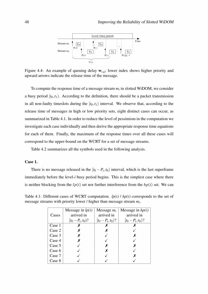
48 Improving the Reliability of Slotted WiDOM
TimeStream m1
Stream m2
q1,0
q2,0
q1,1
q2,1
...
q2,Q2−1
Level-i busy period
Tx
Tx
Tx
Tx Tx
w2,1
Figure 4.4: An example of queuing delay wi,q; lower index shows higher priority andupward arrows indicate the release time of the message.
To compute the response time of a message stream mi in slotted WiDOM, we consider
a busy period [t0, t1). According to the definition, there should be a packet transmission
in all non-faulty timeslots during the [t0, t1) interval. We observe that, according to the
release time of messages in high or low priority sets, eight distinct cases can occur, as
summarized in Table 4.1. In order to reduce the level of pessimism in the computation we
investigate each case individually and then derive the appropriate response time equations
for each of them. Finally, the maximum of the response times over all these cases will
correspond to the upper-bound on the WCRT for a set of message streams.
Table 4.2 summarizes all the symbols used in the following analysis.
Case 1.
There is no message released in the [t0−Ps, t0) interval, which is the last superframe
immediately before the level-i busy period begins. This is the simplest case where there
is neither blocking from the l p(i) set nor further interference from the hp(i) set. We can
Table 4.1: Different cases of WCRT computation. lp(i) / hp(i) corresponds to the set ofmessage streams with priority lower / higher than message stream mi.
Message in lp(i) Message mi Message in hp(i)
Cases arrived in arrived in arrived in[t0−Ps, t0)? [t0−Ps, t0)? [t0−Ps, t0)?
Case 1 ✗ ✗ ✗
Case 2 ✗ ✗ X
Case 3 ✗ X ✗
Case 4 ✗ X X
Case 5 X ✗ ✗
Case 6 X ✗ X
Case 7 X X ✗
Case 8 X X X
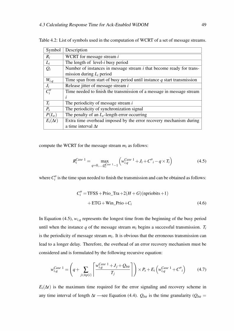
4.3 Calculating Response Time for Ack-Enabled WiDOM 49
Table 4.2: List of symbols used in the computation of WCRT of a set of message streams.
Symbol Description
Ri WCRT for message stream i
Li The length of level-i busy periodQi Number of instances in message stream i that become ready for trans-
mission during Li periodWi,q Time span from start of busy period until instance q start transmissionJi Release jitter of message stream i
C′′i Time needed to finish the transmission of a message in message streami
Ti The periodicity of message stream i
Ps The periodicity of synchronization signalP(Le) The penalty of an Le-length error occurringEi(∆t) Extra time overhead imposed by the error recovery mechanism during
a time interval ∆t
compute the WCRT for the message stream mi as follows:
RCase 1i = max
q=0,...,QCase 1i −1
(
wCase 1i,q + Ji +C′′i−q×Ti
)
(4.5)
where C′′i is the time span needed to finish the transmission and can be obtained as follows:
C′′i =TFSS+Prio_Tra+2(H +G)(npriobits+1)
+ETG+Win_Prio+Ci (4.6)
In Equation (4.5), wi,q represents the longest time from the beginning of the busy period
until when the instance q of the message stream mi begins a successful transmission. Ti
is the periodicity of message stream mi. It is obvious that the erroneous transmission can
lead to a longer delay. Therefore, the overhead of an error recovery mechanism must be
considered and is formulated by the following recursive equation:
wCase 1i,q =
(
q+ ∑j∈hp(i)
⌈
wCase 1i,q + J j +Qbit
Tj
⌉)
×Ps +Ei
(
wCase 1i,q +C′′i
)
(4.7)
Ei(∆t) is the maximum time required for the error signaling and recovery scheme in
any time interval of length ∆t —see Equation (4.4). Qbit is the time granularity (Qbit =

50 Improving the Reliability of Slotted WiDOM
4/250000 = 16µs) [PAT07].
The number of message requests Qi of the message stream mi that become ready for
transmission before the end of the busy period is given by:
Qi =
⌊
LCase 1i + Ji
Ti
⌋
+1 (4.8)
where Li is the length of the longest level-i busy period and can be computed recursively
by:
LCase 1i = ∑
j∈hp(i)∪i
⌈
LCase 1i + J j
Tj
⌉
×Ps +Ei
(
LCase 1i
)
. (4.9)
To investigate the remaining cases, we follow the same reasoning as above and adapt
the analytical formulations as needed. Note that in each case we should replace the ap-
propriate superscript in the response time equations.
Case 2.
There is an instance of the hp(i) message stream released in the [t0−Ps, t0) interval.
This case is rather similar to Case 1 except that we need to consider more interference
imposed by the hp(i) message stream. Therefore, Ri and Qi can be calculated similarly as
Case 1 (Equation (4.5) and Equation (4.8)), but we must consider the following changes
in the computation of wi,q and Li:
wCase 2i,q =(q+ ∑
j∈hp(i)
⌈wCase 2
i,q +Ps + J j +Qbit
Tj⌉)×Ps +Ei(w
Case 2i,q +C′′i ) (4.10)
LCase 2i = ∑
j∈hp(i)∪i
⌈
LCase 2i +Ps + J j
Tj
⌉
×Ps +Ei
(
LCase 2i
)
. (4.11)
Case 3.
In this case, neither hp(i) nor l p(i) messages occur in the [t0−Ps, t0) interval, but
an instance q of the message stream mi is released in [t0−Ps, t0) slightly after the synch

4.3 Calculating Response Time for Ack-Enabled WiDOM 51
signal’s broadcast. As described in Chapter 2, only nodes with non-empty ready queue
wait to receive the synch signal. Thus, the instance q misses participating in the current
tournament phase and should wait for the next superframe. As a consequence, this case
is similar to Case 1, but the duration of an extra superframe must be added into Equa-
tion (4.5), resulting in:
RCase 3i =Ps + max
q=0,...,QCase 3i −1
(
wCase 3i,q + Ji +C′′i−q×Ti
)
. (4.12)
Case 4.
There is no l p(i) message released in the [t0−Ps, t0) interval, but both hp(i) and an
instance q of the message stream mi are released during such interval. With the same
reasoning stated in Case 2, Equation (4.7) and Equation (4.9) are rewritten as follows:
wCase 4i,q =
(
q+ ∑j∈hp(i)
⌈
wCase 4i,q +Ps + J j +Qbit
Tj
⌉)
×Ps +Ei
(
wCase 4i,q +C′′i
)
(4.13)
LCase 4i = ∑
j∈hp(i)∪i
⌈
LCase 4i +Ps + J j
Tj
⌉
×Ps +Ei
(
LCase 4i
)
. (4.14)
Then Ri is expressed as follows:
RCase 4i =Ps + max
q=0,...,QCase 4i −1
(
wCase 4i,q + Ji +C′′i−q×Ti
)
. (4.15)
Case 5.
There is an instance of l p(i) released in the [t0−Ps, t0) interval but no other messages,
neither mi nor hp(i) are released in the same period. Following the same reasoning as in
Case 1, we should revise the computation of wi,q and Li with a blocking term, obtaining:

52 Improving the Reliability of Slotted WiDOM
wCase 5i,q =
(
q+ ∑j∈hp(i)
⌈
wCase 5i,q + J j +Qbit
Tj
⌉
+1
)
×Ps +Ei
(
wCase 5i,q +C′′i
)
(4.16)
LCase 5i =
(
1+ ∑j∈hp(i)∪i
⌈
LCase 5i + J j
Tj
⌉
)
×Ps +Ei
(
LCase 5i
)
. (4.17)
Case 6.
In this case, both hp(i) and l p(i) messages are released within the [t0−Ps, t0) interval.
Knowing that the low priority message is suppressed by the higher priority one, we can
consider this case exactly the same as Case 2 where there is no l p(i) message instance
released.
Case 7.
There is no hp(i) message in the [t0−Ps, t0) interval, but both l p(i) message and an
instance q from message stream mi are released during this interval. It is clear that the
l p(i) message cannot impose any blocking to the response time computations; thus this
case is equivalent to Case 3.
Case 8.
An instance of hp(i), l p(i) and the message stream mi are released within the [t0−Ps, t0)
interval. Following the same rationale as in the last two cases, l p(i) message is suppressed
by higher priority messages, which results in similar equations as in Case 4.
Finally, by looking at all the possible scenarios, and observing that the response time
in Case 4 is greater than or equal to the response times of Case 1, Case 2 and Case 3, the
WCRT of a message stream mi is given by:
Ri = max(
RCase 4i ,RCase 5
i
)
. (4.18)

4.4 Implementation and Practical Aspects 53
4.4 Implementation and Practical Aspects
We implemented the Ack-enabled WiDOM in the Nano-RK operating system [ERR05].
To the best of our knowledge, this is the first reported implementation of WiDOM (either
slotted or unslotted) with an acknowledgement mechanism.
Nano-RK is a Real-Time Operating System (RTOS) designed for wireless sensor net-
works. It employs an energy-efficient time management scheme using one-shot timer
interrupts, instead of polling interrupts. Due to that policy, the scheduler executes with
the periodicity of such timer, i.e., approximately every 1 ms. Consequently, every time-
related events, such as task periods and event wake-ups, will experience at most a 1 ms
jitter with respect to their targeted time. Nevertheless, to enhance the accuracy of our
estimations, jitter has been taken into account into our analytical computations.
Each sender node has three periodic tasks running on Nano-RK: Send-Task; Receive-
Task and Management-Task. The pseudo-code for those tasks are presented as Algo-
rithm 4, Algorithm 5 and Algorithm 6, respectively. At each request of Send-Task the
variable Gnt_N is incremented by one. That variable is used to record the number of re-
quests for packet transmission generated during an experiment. The arrival time of each
Algorithm 4: Send-Task
1 while TRUE do
2 Gnt_T ← keep the current time3 Gnt_N++4 LockSend ← TRUE5 SendPkt()
6 SSentFlag← 0
7 LockSend ← FALSE8 Wait until next period9 end
10 Procedure SendPkt()11 if successful access to hardware=1 and my_ID=winner_ID then
12 if Transmission=original then
13 Txed_N++14 end
15 Transmit the packet over radio16 T T SRCV ← TRUE17 end

54 Improving the Reliability of Slotted WiDOM
request is stored in the variable Gnt_T, in order to check the possibility of retransmissions
in case of an unsuccessful data exchange.
Since the tournament phase is performed by a WiFLEX board, which is shared by two
tasks (Send-Task and Management-Task), the access to that resource needs arbitration.
This has been implemented by regulating the way tasks call a SendPkt() function, through
a global flag (LockSend), which is set by the Send-Task only.
Through the SendPkt() function the nodes start contending for the channel. Based on
the WiDOM protocol, each node uses its given ID number as its packet priority, and if
two or more nodes access the channel at the same time, the collision will be resolved by
the given priorities. As a result, if a node wins the tournament, it sends its packet and
then “activates” the Receive-Task in order to wait for the reception of the corresponding
acknowledgment packet. To do so, it sets a global flag (T T SRCV , time to start receiving)
to TRUE — see Algorithm 4, line 16.
When the Receive-Task executes, one of the following conditions might hold: (i) the
global flag T T SRCV has not been set, so the task suddenly exits, or (ii) the flag has been
set by the Send-Task. In the latter case, the node switches to receive mode and waits to
receive an Ack packet. If the received Ack packet is the expected one, i.e., it contains the
correct information including the source ID and the sequence number of the recent data
transmission, then the global flag “SSentFlag” (i.e., successful sent) will be set to TRUE.
Algorithm 5: Receive-Task
1 while TRUE do
2 if T T SRCV = FALSE then
3 Wait until next period4 else
5 Wait to receive the Ack packet6 if received Ack is correct then
7 SSentFlag← 1
8 end
9 T T SRCV ← FALSE10 T T SMNG ← TRUE11 Wait until next period12 end
13 end

4.4 Implementation and Practical Aspects 55
Algorithm 6: Management-Task
1 while TRUE do
2 if T T SMNG = FALSE then
3 Wait until next period4 else
5 Now← current time6 Elapsed_T ← Now − Gnt_T
7 if Elapsed_T >(Send_Task_period −Ps) and SSentFlag = 0 and LockSend = FALSE
then
8 SendPkt()
9 end
10 T T SMNG← FALSE11 Wait until next period12 end
13 end
Either the Ack has been received or not, the Receive-Task ends up by “activating” the
Management-Task to execute — see Algorithm 5, line 10.
Similarly, the Management-Task encounters one of these two situations when it re-
quests to be executed: (i) the first situation occurs when the “T T SMNG” flag (time to
start managing) is FALSE; in this case the task is released to the scheduler and waits for
the next activation — see Algorithm 6, and (ii) the second situation occurs when the
T T SMNG is TRUE, which usually happens after an unsuccessful transmission of data
packet (i.e. not receiving an Ack packet). Then, if the T T SMNG is TRUE, a retransmis-
sion is needed. The first step for retransmission is to get the current time and check if
there is enough time to perform a retransmission. To do so, it is needed to compute the
elapsed time by subtracting the current time to the Gnt_T time, recorded at the beginning
of the Send-Task. If there is enough time for a slot with duration Ps before the next ac-
tivation of Send-Task (which is defined by the Send-Task period), then it is possible to
retransmit the packet. However, the retransmission should be performed if the SSentFlag
is still FALSE. In this case, the task calls the SendPkt() function, ensuring that the shared
resource is currently available. Taking advantage of locks and flags, we are able to tar-
get an efficient way to control the execution of each task at the appropriate time instant.
Table 4.3 shows the values Nano-RK allows to set for each task’s configuration. A small
number in Task_prio implies higher priority and the period of the Send-Task defines the

56 Improving the Reliability of Slotted WiDOM
data rate of the nodes in each experiment.
Table 4.3: Tasks’ configuration.
Parameter ValueSend_Task_prio 2Send_Task_period MSG-PeriodSend_Task.SchType NON-PREEMPTIVEReceive_Task_prio 3Receive_Task_period 15 msReceive_Task.SchType PREEMPTIVEManagemant_Task_prio 4Managemant_Task_period 15 msManagemant _Task.SchType PREEMPTIVE
When a packet has no chance to be transmitted within its deadline, it is said that a
deadline miss event occurred. In order to estimate how often this happens, at the end of
each experiment, the difference between the number of generated packets (Gnt_N) and
the number of actually transmitted packets (Txed_N) is computed. Similarly, to measure
the response time, each node measures the delay between the instant of the Send-Task
execution until the actual packet transmission. Then, this delay (Wi) piggybacks within
the packet payload. Since we have used a hardware-timer with a time resolution of 1 µs,
all the measured values have the accuracy of 1 µs. Upon receiving a packet, the receiver
extracts the Wi and computes the response time (Ri) according to the following expression:
Ri =Wi +Ci (4.19)
where Ci is the duration of the data exchange phase (refer to Figure 4.1).
With the help of sniffer devices [KCG+11] and a custom-designed log file’s parser,
built in C and bash programming, we were able to measure the packet loss ratio and the
WCRT-miss ratio. Furthermore, to enrich the comparison of the performance between the
original WiDOM and the novel Ack-based protocol, the energy consumed by the nodes at
different data rates is also shown. Finally, to better appreciate the trade-offs between the
performance indices, the behavior of the packet loss ratio against the energy consumption
is presented.
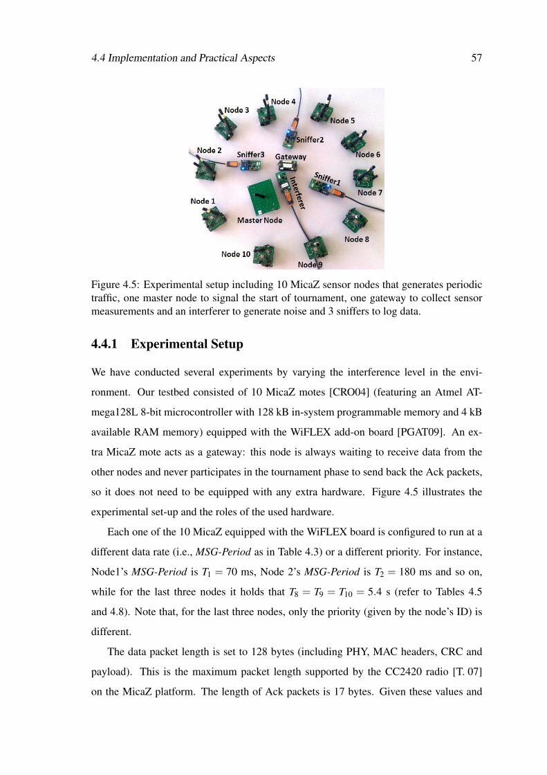
4.4 Implementation and Practical Aspects 57
Figure 4.5: Experimental setup including 10 MicaZ sensor nodes that generates periodictraffic, one master node to signal the start of tournament, one gateway to collect sensormeasurements and an interferer to generate noise and 3 sniffers to log data.
4.4.1 Experimental Setup
We have conducted several experiments by varying the interference level in the envi-
ronment. Our testbed consisted of 10 MicaZ motes [CRO04] (featuring an Atmel AT-
mega128L 8-bit microcontroller with 128 kB in-system programmable memory and 4 kB
available RAM memory) equipped with the WiFLEX add-on board [PGAT09]. An ex-
tra MicaZ mote acts as a gateway: this node is always waiting to receive data from the
other nodes and never participates in the tournament phase to send back the Ack packets,
so it does not need to be equipped with any extra hardware. Figure 4.5 illustrates the
experimental set-up and the roles of the used hardware.
Each one of the 10 MicaZ equipped with the WiFLEX board is configured to run at a
different data rate (i.e., MSG-Period as in Table 4.3) or a different priority. For instance,
Node1’s MSG-Period is T1 = 70 ms, Node 2’s MSG-Period is T2 = 180 ms and so on,
while for the last three nodes it holds that T8 = T9 = T10 = 5.4 s (refer to Tables 4.5
and 4.8). Note that, for the last three nodes, only the priority (given by the node’s ID) is
different.
The data packet length is set to 128 bytes (including PHY, MAC headers, CRC and
payload). This is the maximum packet length supported by the CC2420 radio [T. 07]
on the MicaZ platform. The length of Ack packets is 17 bytes. Given these values and
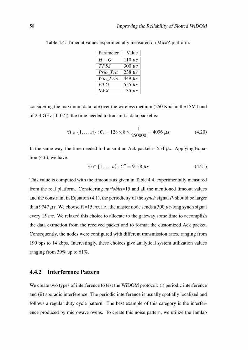
58 Improving the Reliability of Slotted WiDOM
Table 4.4: Timeout values experimentally measured on MicaZ platform.
Parameter Value
H +G 110 µs
T FSS 300 µs
Prio_Tra 238 µs
Win_Prio 449 µs
ET G 555 µs
SWX 35 µs
considering the maximum data rate over the wireless medium (250 Kb/s in the ISM band
of 2.4 GHz [T. 07]), the time needed to transmit a data packet is:
∀i ∈ {1, . . . ,n} : Ci = 128×8× 1
250000= 4096 µs (4.20)
In the same way, the time needed to transmit an Ack packet is 554 µs. Applying Equa-
tion (4.6), we have:
∀i ∈ {1, . . . ,n} : C′′i = 9158 µs (4.21)
This value is computed with the timeouts as given in Table 4.4, experimentally measured
from the real platform. Considering npriobits=15 and all the mentioned timeout values
and the constraint in Equation (4.1), the periodicity of the synch signal Ps should be larger
than 9747 µs. We choose Ps=15 ms, i.e., the master node sends a 300 µs-long synch signal
every 15 ms. We relaxed this choice to allocate to the gateway some time to accomplish
the data extraction from the received packet and to format the customized Ack packet.
Consequently, the nodes were configured with different transmission rates, ranging from
190 bps to 14 kbps. Interestingly, these choices give analytical system utilization values
ranging from 39% up to 61%.
4.4.2 Interference Pattern
We create two types of interference to test the WiDOM protocol: (i) periodic interference
and (ii) sporadic interference. The periodic interference is usually spatially localized and
follows a regular duty cycle pattern. The best example of this category is the interfer-
ence produced by microwave ovens. To create this noise pattern, we utilize the Jamlab
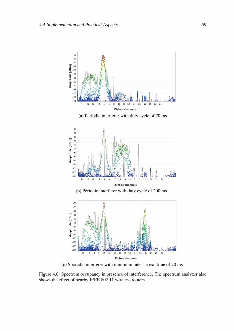
4.4 Implementation and Practical Aspects 59
-50
-55
-60
-65
-70
-75
-80
-85
-90
-95
-100
-105
-110
11 12 13 14 15 16 17 18 19 20 21 22 23 24 25 26
Am
plitu
de [
dB
m]
Zigbee channels
(a) Periodic interferer with duty cycle of 70 ms
-50
-55
-60
-65
-70
-75
-80
-85
-90
-95
-100
-105
-110
11 12 13 14 15 16 17 18 19 20 21 22 23 24 25 26
Am
plitu
de [
dB
m]
Zigbee channels
(b) Periodic interferer with duty cycle of 200 ms.
-50
-55
-60
-65
-70
-75
-80
-85
-90
-95
-100
-105
-110
11 12 13 14 15 16 17 18 19 20 21 22 23 24 25 26
Am
plitu
de [
dB
m]
Zigbee channels
(c) Sporadic interferer with minimum inter-arrival time of 70 ms.
Figure 4.6: Spectrum occupancy in presence of interference. The spectrum analyzer alsoshows the effect of nearby IEEE 802.11 wireless routers.

60 Improving the Reliability of Slotted WiDOM
THNC= 70 ms ≈ PS
HNC
Time
TLNC= 200 ms ≈ PS
LNC
Time
Interference burst Interference free
Tx
Tx Re-Tx
Re-Tx
Tx Re-Tx Tx Re-Tx Tx Re-Tx
Tx Tx Re-Tx Re-Tx Tx
Transmit request Retransmit request
Stream mi
Stream mi
Figure 4.7: Example of data transmission under HNC and LNC interference.
tool [BVN+11] running on an extra MicaZ node (“interferer” node in Figure 4.5). We
set the interferer’s duty cycle to 70 ms and 200 ms to compare the performance of the
WiDOM protocol under different noise densities. We refer to the environment with higher
noise burst rate as the High Noisy Channel (HNC) scenario —see Figure 4.6 (a), and the
one with with lower noise burst rate as the Low Noisy Channel (LNC) scenario —see
Figure 4.6 (b). Both periodic interferers send three packets with length of 128 bytes in
burst to occupy the channel for the duration of one slot, Ps=15 ms —considering data rate
of 250 Kb/s.
Figure 4.7 aims at clarifying, with an example, how the HNC and LNC channel con-
ditions impact on the message stream transmissions. The message streams have the same
data rate in both scenarios, i.e., the transmit requests generation time is the same. Clearly,
the HNC scenario leads to more collisions than the LNC one, thus more frequent retrans-
missions.
The sporadic noise model emulates in a fully controlled way the interference gener-
ated by heavily loaded Wi-Fi access points. To generate this type of interference traffic,
we used a simple model, inspired by the Markov model presented in [BVT+10], con-
sisting of two states: “clear channel” and “interference”. Differently from the Jamlab
tool [BVT+10], in our model, instead of considering fully random and irregular interfer-
ence pattern, we generate a fixed duration of “interference” to keep the burst length equal
to one Ps period. In this state, the interferer broadcasts unmodulated signals. The duration
of the “clear channel” state is defined through a constant slot 5 ms duration multiplied by

4.4 Implementation and Practical Aspects 61
a random variable R, uniformly distributed over the interval [14,200] ms. Hence, the time
duration of staying on the clear channel state will be a random time period from 70 ms
up to 1 s. In other words, the minimum inter-arrival time between two consecutive noise
bursts is set to 70 ms. We refer to this scenario as the Sporadic Noisy Channel (SPNC)
scenario —see Figure 4.6 (c).
All interferers generate noise in the Channel 15 of the IEEE 802.15.4 spectrum. In
all scenarios, interferers are generating packets and transmitting them with the highest
power level (0 dBm). As it is shown by the spectrum analyzer (Figure 4.6), the radiation
power in all situations is the same, but the density of noise bursts is quite high in the
Figure 4.6 (a) as compared to that in Figure 4.6 (b). It can be also observed that in the
presence of a sporadic noise source, the channel spends more time in clear channel state
as compared to the periodic noise source with duty cycle of 70 ms. Note that the spectrum
analyzer visualizes the status of the entire ZigBee bandwidth, including the noise coming
from WiFi/IEEE 802.11 wireless routers on the adjacent channels.
4.4.3 Evaluation
We utilize different interference patterns to evaluate the reliability and the robustness of
the WiDOM protocol against noise, while having a predictable response time for message
streams. Our evaluation focuses on five network performance indices as indicated next.
Packet loss ratio: the ratio of the data (measurements) missed in the gateway over
total number of the generated data by sender nodes.
Deadline miss ratio: the ratio of messages that missed their deadlines over the total
number of generated messages. In all scenarios, the deadline is considered to be implicit
which is equal to the message periodicity.
WCRT miss ratio: the ratio of messages that have been sent after their calculated
WCRT over the total number of generated messages.

62 Improving the Reliability of Slotted WiDOM
Average response time: the average of all received messages response time in the
gateway from any sender.
Energy consumption: the average energy consumption of each node, expressed as a
function of the number of packets sent and received.
We run the experiment for both the original and the Ack-enabled versions of WiDOM in
different noisy environments. All experiments were run for about 40 minutes, which cor-
responds to more than 40000 message transmission requests.
4.4.3.1 Packet Loss Ratio
Figure 4.8 depicts the packet loss ratio for both versions of the WiDOM protocol, under
different noise conditions. According to the results, two observations can be made. First,
the packet loss ratio for the Ack-enabled WiDOM is much smaller than that of the original
version of the WiDOM protocol in all scenarios. This is due to the implementation of Ack
packets, which provide a legitimate feedback on transmission status for the sender nodes,
giving them a chance for retransmitting the lost packets.
Second, the high noisy channel (HNC) jeopardizes the network performance much
more than the low noisy channel or the SPNC case. As it is illustrated in Figure 4.8,
SPNC is less destructive, since the packet loss ratio under SPNC is lower than the one
under HNC for both WiDOM versions. Two reasons contribute to this: (i) in heavy noisy
channels there is a higher risk of collision for both data and Ack packets; and (ii) a higher
collision rate inherently leads to more retransmission requests in the case of Ack-enabled
WiDOM, which increases the traffic load.
Moreover, in each scenario the packet loss ratio is almost flat against the data rate.
One could think that for higher transmission rates there ought to be higher amounts of
packet loss. Indeed, this happens in absolute terms, but in terms of packet loss ratio (i.e.,
percentage), the effect is minimal.
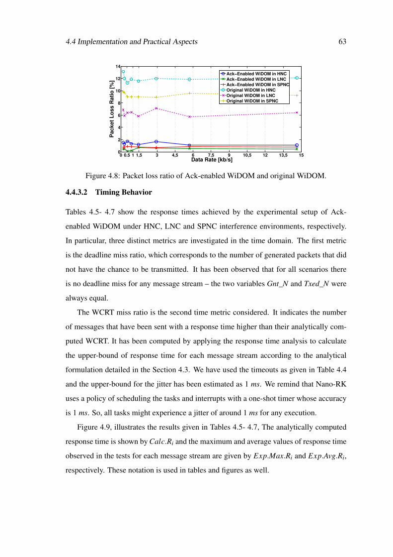
4.4 Implementation and Practical Aspects 63
0 0.5 1 1,5 3 4,5 6 7,5 9 10,5 12 13,5 150
2
4
6
8
10
12
14
Data Rate [kb/s]
Pa
ck
et
Lo
ss
Ra
tio
[%
]
Ack−Enabled WiDOM in HNC
Ack−Enabled WiDOM in LNC
Ack−Enabled WiDOM in SPNC
Original WiDOM in HNC
Original WiDOM in LNC
Original WiDOM in SPNC
Figure 4.8: Packet loss ratio of Ack-enabled WiDOM and original WiDOM.
4.4.3.2 Timing Behavior
Tables 4.5- 4.7 show the response times achieved by the experimental setup of Ack-
enabled WiDOM under HNC, LNC and SPNC interference environments, respectively.
In particular, three distinct metrics are investigated in the time domain. The first metric
is the deadline miss ratio, which corresponds to the number of generated packets that did
not have the chance to be transmitted. It has been observed that for all scenarios there
is no deadline miss for any message stream – the two variables Gnt_N and Txed_N were
always equal.
The WCRT miss ratio is the second time metric considered. It indicates the number
of messages that have been sent with a response time higher than their analytically com-
puted WCRT. It has been computed by applying the response time analysis to calculate
the upper-bound of response time for each message stream according to the analytical
formulation detailed in the Section 4.3. We have used the timeouts as given in Table 4.4
and the upper-bound for the jitter has been estimated as 1 ms. We remind that Nano-RK
uses a policy of scheduling the tasks and interrupts with a one-shot timer whose accuracy
is 1 ms. So, all tasks might experience a jitter of around 1 ms for any execution.
Figure 4.9, illustrates the results given in Tables 4.5- 4.7, The analytically computed
response time is shown by Calc.Ri and the maximum and average values of response time
observed in the tests for each message stream are given by Exp.Max.Ri and Exp.Avg.Ri,
respectively. These notation is used in tables and figures as well.
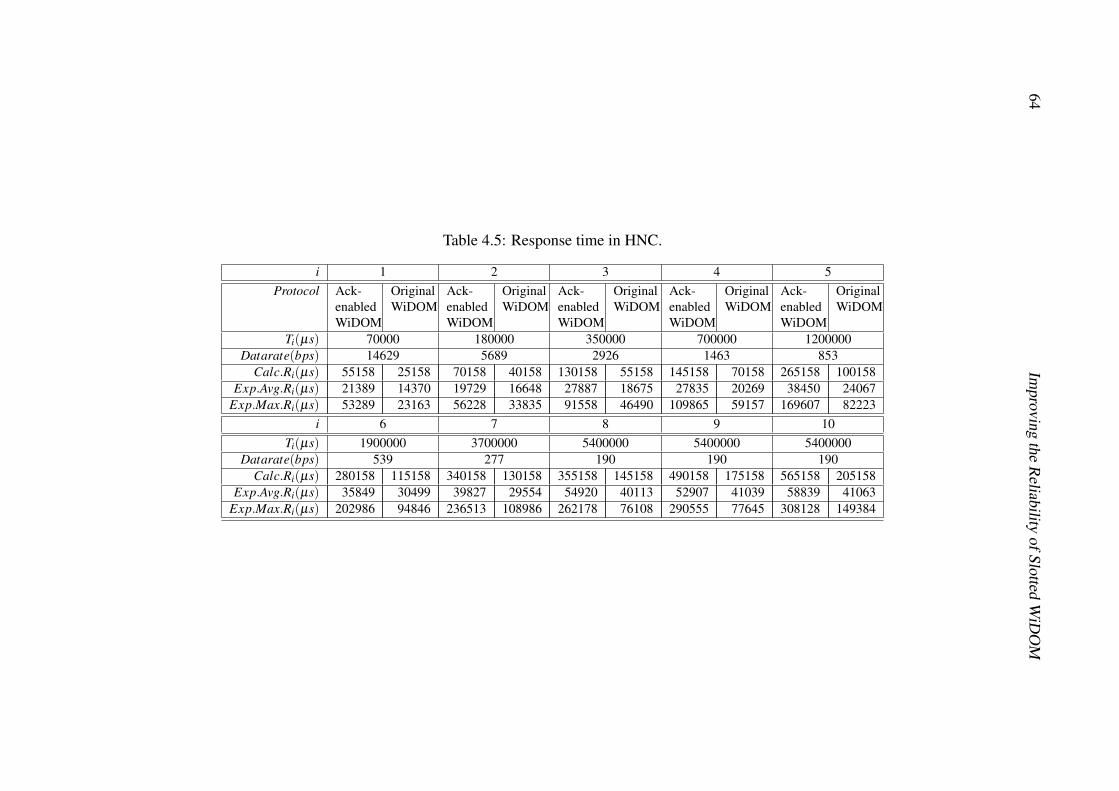
64Im
pro
vin
gth
eR
eliability
of
Slo
ttedW
iDO
M
Table 4.5: Response time in HNC.
i 1 2 3 4 5
Protocol Ack-enabledWiDOM
OriginalWiDOM
Ack-enabledWiDOM
OriginalWiDOM
Ack-enabledWiDOM
OriginalWiDOM
Ack-enabledWiDOM
OriginalWiDOM
Ack-enabledWiDOM
OriginalWiDOM
Ti(µs) 70000 180000 350000 700000 1200000Datarate(bps) 14629 5689 2926 1463 853
Calc.Ri(µs) 55158 25158 70158 40158 130158 55158 145158 70158 265158 100158Exp.Avg.Ri(µs) 21389 14370 19729 16648 27887 18675 27835 20269 38450 24067
Exp.Max.Ri(µs) 53289 23163 56228 33835 91558 46490 109865 59157 169607 82223
i 6 7 8 9 10
Ti(µs) 1900000 3700000 5400000 5400000 5400000Datarate(bps) 539 277 190 190 190
Calc.Ri(µs) 280158 115158 340158 130158 355158 145158 490158 175158 565158 205158Exp.Avg.Ri(µs) 35849 30499 39827 29554 54920 40113 52907 41039 58839 41063
Exp.Max.Ri(µs) 202986 94846 236513 108986 262178 76108 290555 77645 308128 149384
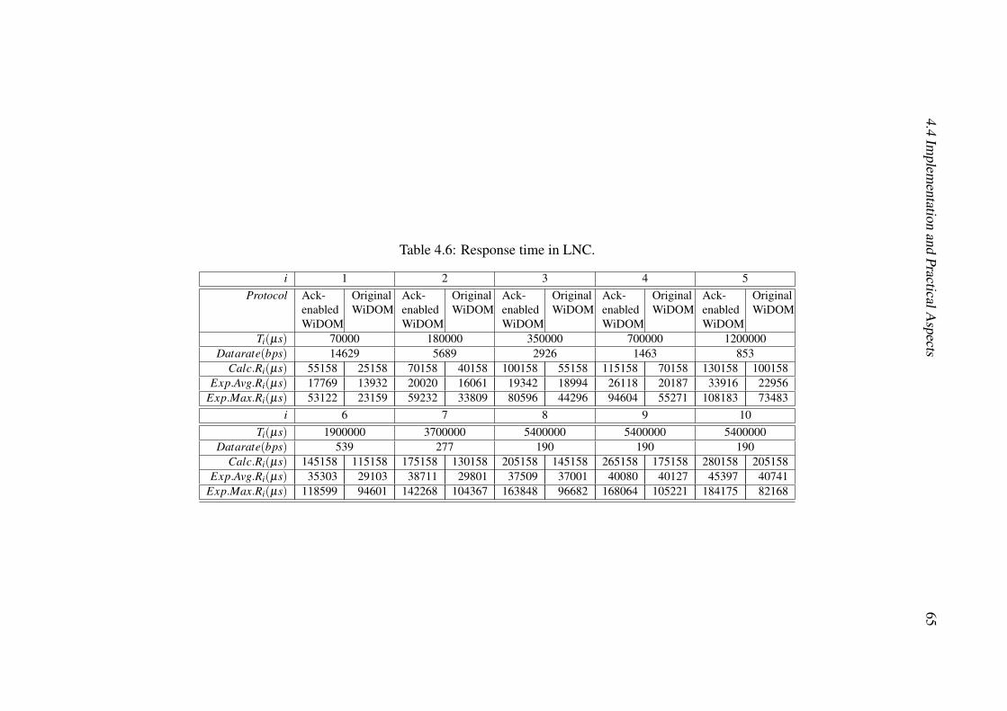
4.4
Implem
entatio
nan
dP
racticalA
spects
65
Table 4.6: Response time in LNC.
i 1 2 3 4 5
Protocol Ack-enabledWiDOM
OriginalWiDOM
Ack-enabledWiDOM
OriginalWiDOM
Ack-enabledWiDOM
OriginalWiDOM
Ack-enabledWiDOM
OriginalWiDOM
Ack-enabledWiDOM
OriginalWiDOM
Ti(µs) 70000 180000 350000 700000 1200000Datarate(bps) 14629 5689 2926 1463 853
Calc.Ri(µs) 55158 25158 70158 40158 100158 55158 115158 70158 130158 100158Exp.Avg.Ri(µs) 17769 13932 20020 16061 19342 18994 26118 20187 33916 22956
Exp.Max.Ri(µs) 53122 23159 59232 33809 80596 44296 94604 55271 108183 73483
i 6 7 8 9 10
Ti(µs) 1900000 3700000 5400000 5400000 5400000Datarate(bps) 539 277 190 190 190
Calc.Ri(µs) 145158 115158 175158 130158 205158 145158 265158 175158 280158 205158Exp.Avg.Ri(µs) 35303 29103 38711 29801 37509 37001 40080 40127 45397 40741
Exp.Max.Ri(µs) 118599 94601 142268 104367 163848 96682 168064 105221 184175 82168
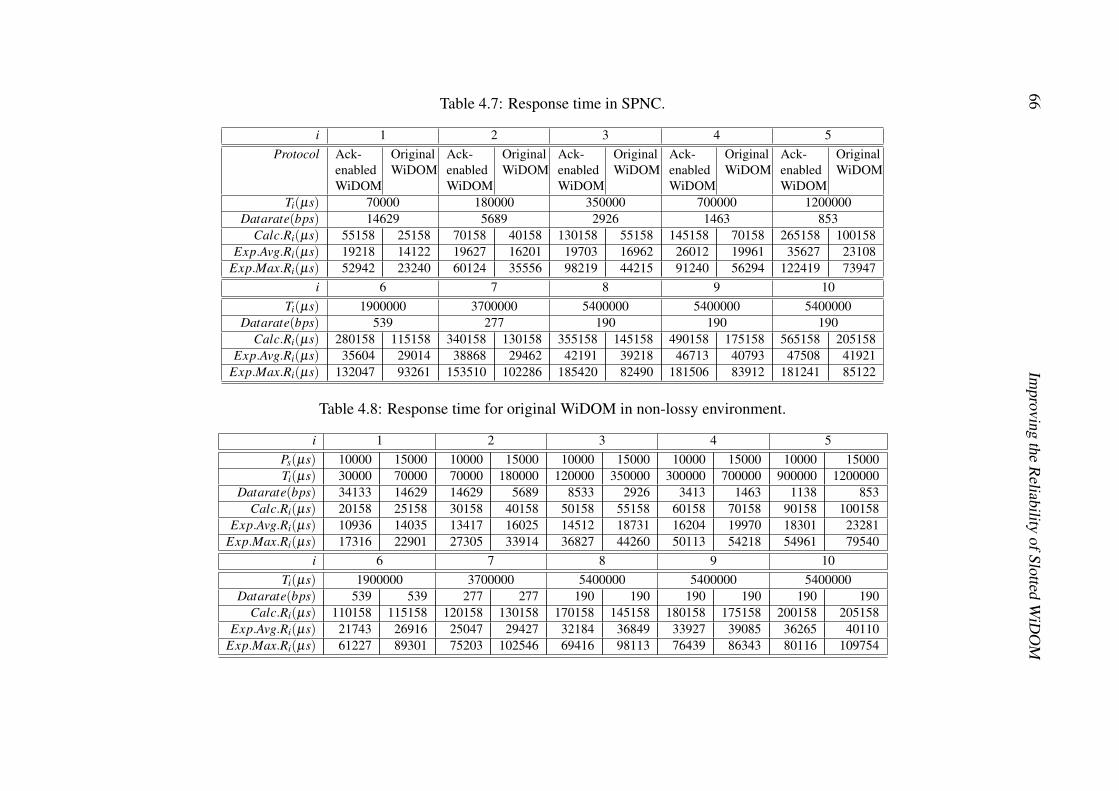
66Im
pro
vin
gth
eR
eliability
of
Slo
ttedW
iDO
M
Table 4.7: Response time in SPNC.
i 1 2 3 4 5
Protocol Ack-enabledWiDOM
OriginalWiDOM
Ack-enabledWiDOM
OriginalWiDOM
Ack-enabledWiDOM
OriginalWiDOM
Ack-enabledWiDOM
OriginalWiDOM
Ack-enabledWiDOM
OriginalWiDOM
Ti(µs) 70000 180000 350000 700000 1200000Datarate(bps) 14629 5689 2926 1463 853
Calc.Ri(µs) 55158 25158 70158 40158 130158 55158 145158 70158 265158 100158Exp.Avg.Ri(µs) 19218 14122 19627 16201 19703 16962 26012 19961 35627 23108
Exp.Max.Ri(µs) 52942 23240 60124 35556 98219 44215 91240 56294 122419 73947
i 6 7 8 9 10
Ti(µs) 1900000 3700000 5400000 5400000 5400000Datarate(bps) 539 277 190 190 190
Calc.Ri(µs) 280158 115158 340158 130158 355158 145158 490158 175158 565158 205158Exp.Avg.Ri(µs) 35604 29014 38868 29462 42191 39218 46713 40793 47508 41921
Exp.Max.Ri(µs) 132047 93261 153510 102286 185420 82490 181506 83912 181241 85122
Table 4.8: Response time for original WiDOM in non-lossy environment.
i 1 2 3 4 5
Ps(µs) 10000 15000 10000 15000 10000 15000 10000 15000 10000 15000Ti(µs) 30000 70000 70000 180000 120000 350000 300000 700000 900000 1200000
Datarate(bps) 34133 14629 14629 5689 8533 2926 3413 1463 1138 853Calc.Ri(µs) 20158 25158 30158 40158 50158 55158 60158 70158 90158 100158
Exp.Avg.Ri(µs) 10936 14035 13417 16025 14512 18731 16204 19970 18301 23281Exp.Max.Ri(µs) 17316 22901 27305 33914 36827 44260 50113 54218 54961 79540
i 6 7 8 9 10
Ti(µs) 1900000 3700000 5400000 5400000 5400000Datarate(bps) 539 539 277 277 190 190 190 190 190 190
Calc.Ri(µs) 110158 115158 120158 130158 170158 145158 180158 175158 200158 205158Exp.Avg.Ri(µs) 21743 26916 25047 29427 32184 36849 33927 39085 36265 40110
Exp.Max.Ri(µs) 61227 89301 75203 102546 69416 98113 76439 86343 80116 109754

4.4 Implementation and Practical Aspects 67
0
100
200
300
400
500
600
1 2 3 4 5 6 7 8 9 10
Resp
on
se t
ime (
ms)
Node ID
Calc. Ri
Exp. Avg. Ri
Exp. Max. Ri
(a) Ack-enabled WiDOM in HNC environment.
0
50
100
150
200
250
1 2 3 4 5 6 7 8 9 10
Resp
on
se t
ime (
ms)
Node ID
Calc. Ri
Exp. Avg. Ri
Exp. Max. Ri
(b) Original WiDOM in HNC environment.
0
50
100
150
200
250
300
1 2 3 4 5 6 7 8 9 10
Resp
on
se t
ime (
ms)
Node ID
Calc. Ri
Exp. Avg. Ri
Exp. Max. Ri
(c) Ack-enabled WiDOM in LNC environment.
0
50
100
150
200
250
1 2 3 4 5 6 7 8 9 10
Resp
on
se t
ime (
ms)
Node ID
Calc. Ri
Exp. Avg. Ri
Exp. Max. Ri
(d) Original WiDOM in LNC environment.
0
100
200
300
400
500
600
1 2 3 4 5 6 7 8 9 10
Resp
on
se t
ime (
ms)
Node ID
Calc. Ri
Exp. Avg. Ri
Exp. Max. Ri
(e) Ack-enabled WiDOM in SPNC environment.
0
50
100
150
200
250
1 2 3 4 5 6 7 8 9 10
Resp
on
se t
ime (
ms)
Node ID
Calc. Ri
Exp. Avg. Ri
Exp. Max. Ri
(f) Original WiDOM in SPNC environment.
Figure 4.9: Response time comparison of Ack-enabled WiDOM and original WiDOM un-der different noise conditions.
Figure 4.9, clearly shows that no message experiences a response time higher than
the calculated WCRT in all the considered scenarios, which substantiates the fact that
the analytical model for the WCRT provides a fairly good upper-bound to the expected
response time.
The average value of response time, Exp.Avg.Ri, is the third and last metric consid-
ered in the timing category. It clearly shows how the Ack-enabled mechanism slightly
increases the response time for all the message streams.
As expected, this is what the system pays to achieve the good results in terms of packet

68 Improving the Reliability of Slotted WiDOM
10.936'
13.417'
14.512'16.204'
18.301'
21.743'25.047'
32.184'
33.927'
36.265'
0
50
100
150
200
250
1 2 3 4 5 6 7 8 9 10
Re
sp
on
se
tim
e (
ms
)
Node ID
Calc. Ri
Exp. Avg. Ri
Exp. Max. Ri
(a) Original WiDOM with Ps = 10 ms.
14.035'16.025'
18.731'19.97'
23.281'
26.916'29.427'
36.849'39.085'
40.11'
0
50
100
150
200
250
1 2 3 4 5 6 7 8 9 10
Re
sp
on
se
tim
e (
ms
)
Node ID
Calc. Ri
Exp. Avg. Ri
Exp. Max. Ri
(b) Original WiDOM with Ps = 15 ms.
Figure 4.10: Response time comparison of original WiDOM with different Ps in a non-lossy environment. The numbers indicate the value of the average response time.
loss ratio (as shown in Figure 4.8). Moreover, while the original WiDOM is almost indif-
ferent to the various noise patterns, from the experimental results shown in the tables it
can be observed that heavier noise leads to larger response times for the Ack-enabled slot-
ted WiDOM. These results are not surprising since, as the noise density increases more
packet collisions occur and consequently a higher number of retransmissions. Accord-
ingly, for the original WiDOM, the average response time of message streams does not
vary significantly with the channel conditions. The reason is that there is no mechanism
devised in original WiDOM that takes into account the noise of the channel. Nodes send
their packet only once according to their arrival schedules and there is no feedback to let
them know about their transmission status.
The last observation led us to run another experiment for the original WiDOM in a
non-lossy environment, in order to push the system to its limits. Since we are using the
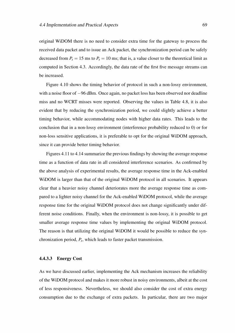
4.4 Implementation and Practical Aspects 69
original WiDOM there is no need to consider extra time for the gateway to process the
received data packet and to issue an Ack packet, the synchronization period can be safely
decreased from Ps = 15 ms to Ps = 10 ms; that is, a value closer to the theoretical limit as
computed in Section 4.3. Accordingly, the data rate of the first five message streams can
be increased.
Figure 4.10 shows the timing behavior of protocol in such a non-lossy environment,
with a noise floor of−96 dBm. Once again, no packet loss has been observed nor deadline
miss and no WCRT misses were reported. Observing the values in Table 4.8, it is also
evident that by reducing the synchronization period, we could slightly achieve a better
timing behavior, while accommodating nodes with higher data rates. This leads to the
conclusion that in a non-lossy environment (interference probability reduced to 0) or for
non-loss sensitive applications, it is preferable to opt for the original WiDOM approach,
since it can provide better timing behavior.
Figures 4.11 to 4.14 summarize the previous findings by showing the average response
time as a function of data rate in all considered interference scenarios. As confirmed by
the above analysis of experimental results, the average response time in the Ack-enabled
WiDOM is larger than that of the original WiDOM protocol in all scenarios. It appears
clear that a heavier noisy channel deteriorates more the average response time as com-
pared to a lighter noisy channel for the Ack-enabled WiDOM protocol, while the average
response time for the original WiDOM protocol does not change significantly under dif-
ferent noise conditions. Finally, when the environment is non-lossy, it is possible to get
smaller average response time values by implementing the original WiDOM protocol.
The reason is that utilizing the original WiDOM it would be possible to reduce the syn-
chronization period, Ps, which leads to faster packet transmission.
4.4.3.3 Energy Cost
As we have discussed earlier, implementing the Ack mechanism increases the reliability
of the WiDOM protocol and makes it more robust in noisy environments, albeit at the cost
of less responsiveness. Nevertheless, we should also consider the cost of extra energy
consumption due to the exchange of extra packets. In particular, there are two major
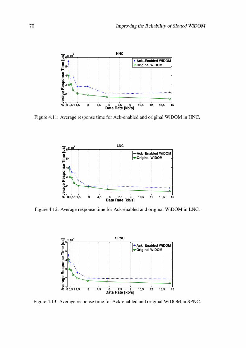
70 Improving the Reliability of Slotted WiDOM
0 0,5 1 1,5 3 4,5 6 7,5 9 10,5 12 13,5 151
2
3
4
5
6x 10
4
Data Rate [kb/s]
Avera
ge R
esp
on
se T
ime [
us] HNC
Ack−Enabled WiDOM
Original WiDOM
Figure 4.11: Average response time for Ack-enabled and original WiDOM in HNC.
0 0,5 1 1,5 3 4,5 6 7,5 9 10,5 12 13,5 151
2
3
4
5
6x 10
4
Data Rate [kb/s]
Avera
ge R
esp
on
se T
ime [
us] LNC
Ack−Enabled WiDOM
Original WiDOM
Figure 4.12: Average response time for Ack-enabled and original WiDOM in LNC.
0 0,5 1 1,5 3 4,5 6 7,5 9 10,5 12 13,5 151
2
3
4
5
6x 10
4
Data Rate [kb/s]
Avera
ge R
esp
on
se T
ime [
us] SPNC
Ack−Enabled WiDOM
Original WiDOM
Figure 4.13: Average response time for Ack-enabled and original WiDOM in SPNC.
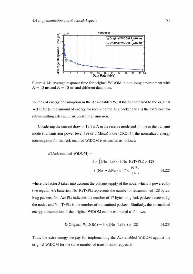
4.4 Implementation and Practical Aspects 71
0 3 6 9 12 15 18 21 24 27 30 33 351
1.5
2
2.5
3
3.5
4x 10
4
Data Rate [kb/s]
Avera
ge R
esp
on
se T
ime [
us] NonLossy
Original WiDOM Ps=10 ms
Original WiDOM Ps=15 ms
Figure 4.14: Average response time for original WiDOM in non-lossy environment withPs = 15 ms and Ps = 10 ms and different data rates.
sources of energy consumption in the Ack-enabled WiDOM as compared to the original
WiDOM: (i) the amount of energy for receiving the Ack packet and (ii) the extra cost for
retransmitting after an unsuccessful transmission.
Cosidering the current draw of 19.7 mA in the receive mode and 14 mA in the transmit
mode (transmission power level 19) of a MicaZ mote [CRO04], the normalized energy
consumption for the Ack-enabled WiDOM is estimated as follows:
E(Ack-enabled WiDOM) =
3×(
(No_TxPkt+No_ReTxPkt)×128
+(No_AckPkt)×17× 19.7
14
)
(4.22)
where the factor 3 takes into account the voltage supply of the node, which is powered by
two regular AA batteries. No_ReTxPkt represents the number of retransmitted 128 bytes-
long packets, No_AckPkt indicates the number of 17 bytes-long Ack packets received by
the nodes and No_TxPkt is the number of transmitted packets. Similarly, the normalized
energy consumption of the original WiDOM can be estimated as follows:
E(Original-WiDOM) = 3× (No_TxPkt)×128 (4.23)
Thus, the extra energy we pay for implementing the Ack-enabled WiDOM against the
original WiDOM for the same number of transmission request is:

72 Improving the Reliability of Slotted WiDOM
Energylossratio[%] =
100× E(Ack-enabled WiDOM)−E(Original-WiDOM)
E(Original-WiDOM)=
100× No_ReTxPkt×128+No_AckPkt×17× 19.714
128×No_TxPkt(4.24)
We do not consider the extra cost paid by the gateway node to receive retransmissions
and to send back the Ack packets. This makes sense under the common assumption that
the gateway is provided with a continuous energy supply.
As it is shown in Figure 4.15, the extra energy cost of using the Ack-enabled mecha-
nism as compared to the original WiDOM roughly ranges between 25% and 35%, for any
data rate. In particular, the energy loss shows some fluctuations at a lower data rates and
tends to stabilize as the data rate increases. The reason is that nodes at lower data rates
may have the opportunity to experience disruptive bursts of interference more often than
the others, and therefore they might need to retransmit more frequently to successfully
deliver their messages.
In terms of interference impact, it is evident that the higher noise density conditions
impose higher energy consumptions due to the higher number of retransmissions. The
energy loss rate is about 10% higher for the HNC scenario as compared to that in LNC
environment, while the SPNC case shows a performance similar to that with the LNC
0 0,5 1 1,5 3 4,5 6 7,5 9 10,5 12 13,5 150
5
10
15
20
25
30
35
40
Data Rate [kb/s]
En
erg
y L
os
s R
ati
o [
%]
HNC
LNC
SPNC
Figure 4.15: Energy loss ratio for Ack-enabled WiDOM vs. original WiDOM in HNC,LNC and SPNC environments.

4.5 Concluding Remarks 73
5000 5500 6000 6500 7000 75000
2
4
6
8
10
12
14
HNC
SPNC
LNC
HNCSPNC
LNC
Average Energy Consumption per Packet [mJ]
Packet
Lo
ss R
ati
o [
%]
Original WiDom
Ack−enabled WiDom
Figure 4.16: Packet loss ratio vs. average energy cost per packet for Ack-enabledWiDOM and original WiDOM under HNC, LNC and SPNC environments.
interference pattern.
Finally, to further examine the impact of the Ack-based mechanism, the packet loss
ratio is plotted against the energy consumption per packet (see Figure 4.16). The energy
consumption has been computed using the expressions for E(Ack-enabled WiDOM) and
E(Original-WiDOM) as previously defined, normalized with respect to the number of
transmitted packets, instead of the transmission current. As expected, the energy con-
sumption of WiDOM is not affected by the interference level, while in the case of the
Ack-enabled WiDOM is. This supports our claim that at the cost of roughly 30% more
energy, it is possible to achieve a reduction of 90% in the packet loss ratio, i.e., keep it
below (2%), regardless of the considered interference.
4.5 Concluding Remarks
In this section, we focused on the reliability of the WiDOM protocol. Our primary con-
tribution was to offer an error recovery scheme to make the protocol more robust and
reliable under noisy conditions. Another contribution of this section was to provide a
novel response time analysis for the slotted WiDOM with message streams that suffer
from release jitter and experience noisy channel conditions. We have shown that our
analysis is non-trivial due to the slotted nature of the protocol. In order to reduce the
level of pessimism in the calculated upper-bound, we individually explored all the possi-
ble cases that may happen according to the arrival pattern of message streams and then

74 Improving the Reliability of Slotted WiDOM
picked the maximum upper-bound among all the possible cases.
To validate our calculated upper-bounds, we conducted a set of experiments under dif-
ferent noisy channel conditions. The experimental results have shown that implementing
the Ack-enabled WiDOM reduces remarkably the packet loss rate to less than 2% even
under high noisy channel as compared to the original WiDOM protocol. The experimen-
tal results also confirmed our analytical findings that the theoretical analysis offer valid
upper-bound for each message streams.
Chapter 5
Self-Adaptive Approximate
Interpolation scheme
In this chapter, we will propose a more efficient scalable data acquisition method for
densely instrumented cyber-physical systems (CPS). Previous research works have pro-
posed approaches for obtaining an approximate interpolation of sensor readings that are
based on dominance protocols. Considering the dominance-based protocol, we design a
new approach that offers a more accurate approximate interpolation by integrating the dy-
namics of the monitored signals into the computational process. We show that through a
self-assessment functionality the algorithm detects sudden changes in the physical model
and adapts itself accordingly.
5.1 Motivation
Recent advances in technology make it feasible to mass produce small sensor devices
with sensing, computation and communication capabilities. These low-power wireless de-
vices can also be powered by the energy scavenged from ambient radio waves [TRNA14].
These capabilities have enabled the integration of physical processes and computing, and
spurred a new direction of research that envisioned massive deployments of networked
embedded computing devices.
75
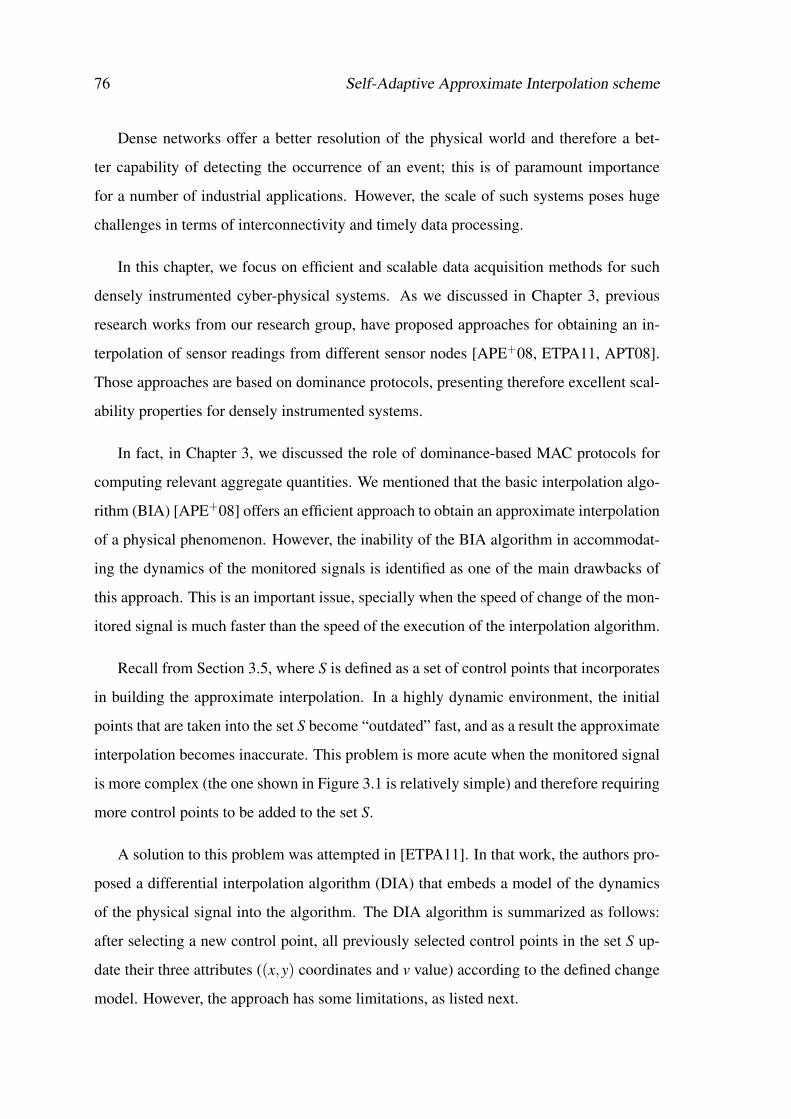
76 Self-Adaptive Approximate Interpolation scheme
Dense networks offer a better resolution of the physical world and therefore a bet-
ter capability of detecting the occurrence of an event; this is of paramount importance
for a number of industrial applications. However, the scale of such systems poses huge
challenges in terms of interconnectivity and timely data processing.
In this chapter, we focus on efficient and scalable data acquisition methods for such
densely instrumented cyber-physical systems. As we discussed in Chapter 3, previous
research works from our research group, have proposed approaches for obtaining an in-
terpolation of sensor readings from different sensor nodes [APE+08, ETPA11, APT08].
Those approaches are based on dominance protocols, presenting therefore excellent scal-
ability properties for densely instrumented systems.
In fact, in Chapter 3, we discussed the role of dominance-based MAC protocols for
computing relevant aggregate quantities. We mentioned that the basic interpolation algo-
rithm (BIA) [APE+08] offers an efficient approach to obtain an approximate interpolation
of a physical phenomenon. However, the inability of the BIA algorithm in accommodat-
ing the dynamics of the monitored signals is identified as one of the main drawbacks of
this approach. This is an important issue, specially when the speed of change of the mon-
itored signal is much faster than the speed of the execution of the interpolation algorithm.
Recall from Section 3.5, where S is defined as a set of control points that incorporates
in building the approximate interpolation. In a highly dynamic environment, the initial
points that are taken into the set S become “outdated” fast, and as a result the approximate
interpolation becomes inaccurate. This problem is more acute when the monitored signal
is more complex (the one shown in Figure 3.1 is relatively simple) and therefore requiring
more control points to be added to the set S.
A solution to this problem was attempted in [ETPA11]. In that work, the authors pro-
posed a differential interpolation algorithm (DIA) that embeds a model of the dynamics
of the physical signal into the algorithm. The DIA algorithm is summarized as follows:
after selecting a new control point, all previously selected control points in the set S up-
date their three attributes ((x,y) coordinates and v value) according to the defined change
model. However, the approach has some limitations, as listed next.
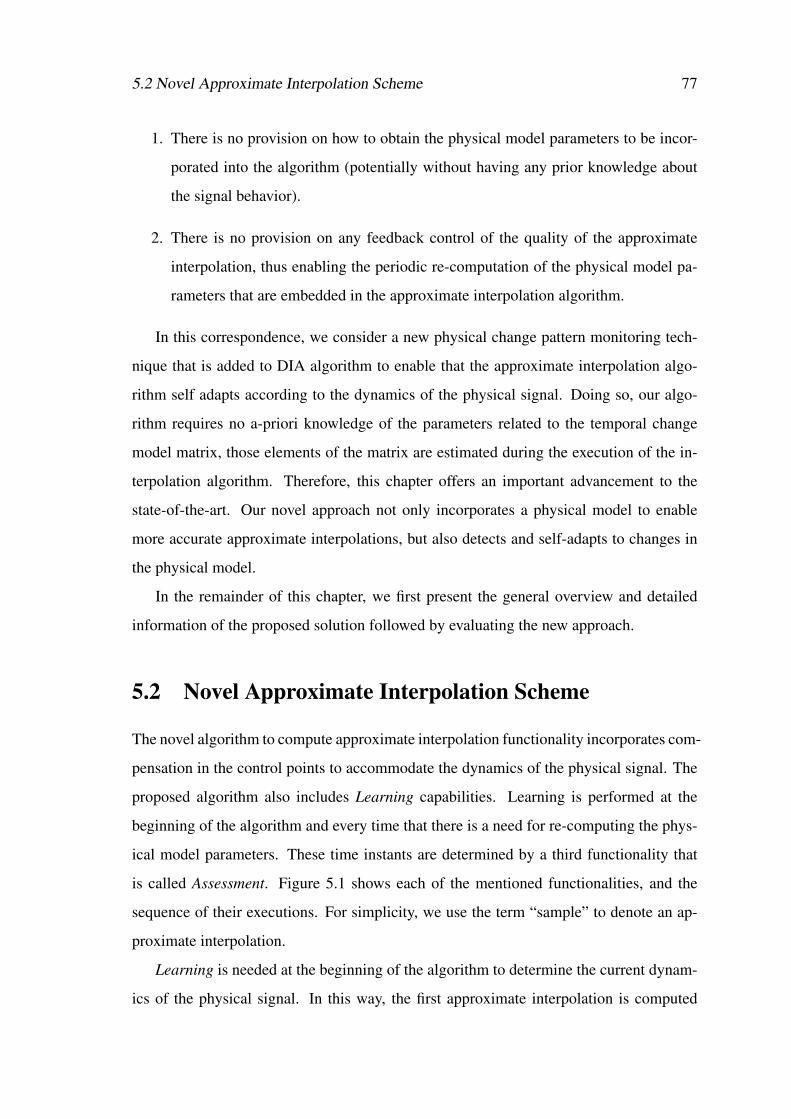
5.2 Novel Approximate Interpolation Scheme 77
1. There is no provision on how to obtain the physical model parameters to be incor-
porated into the algorithm (potentially without having any prior knowledge about
the signal behavior).
2. There is no provision on any feedback control of the quality of the approximate
interpolation, thus enabling the periodic re-computation of the physical model pa-
rameters that are embedded in the approximate interpolation algorithm.
In this correspondence, we consider a new physical change pattern monitoring tech-
nique that is added to DIA algorithm to enable that the approximate interpolation algo-
rithm self adapts according to the dynamics of the physical signal. Doing so, our algo-
rithm requires no a-priori knowledge of the parameters related to the temporal change
model matrix, those elements of the matrix are estimated during the execution of the in-
terpolation algorithm. Therefore, this chapter offers an important advancement to the
state-of-the-art. Our novel approach not only incorporates a physical model to enable
more accurate approximate interpolations, but also detects and self-adapts to changes in
the physical model.
In the remainder of this chapter, we first present the general overview and detailed
information of the proposed solution followed by evaluating the new approach.
5.2 Novel Approximate Interpolation Scheme
The novel algorithm to compute approximate interpolation functionality incorporates com-
pensation in the control points to accommodate the dynamics of the physical signal. The
proposed algorithm also includes Learning capabilities. Learning is performed at the
beginning of the algorithm and every time that there is a need for re-computing the phys-
ical model parameters. These time instants are determined by a third functionality that
is called Assessment. Figure 5.1 shows each of the mentioned functionalities, and the
sequence of their executions. For simplicity, we use the term “sample” to denote an ap-
proximate interpolation.
Learning is needed at the beginning of the algorithm to determine the current dynam-
ics of the physical signal. In this way, the first approximate interpolation is computed

78 Self-Adaptive Approximate Interpolation scheme
No
No
compute transform matrix
compute one sample
Yes
Yes
need re-compute
Tmatrix?
assessment
time?
perform assessment
Yes
No
wait for
TS
Learning
Interpolation
Assessment
sampling time?
Begin
Figure 5.1: The proposed self-adaptive algorithm with Learning and Assessment func-tionalities.
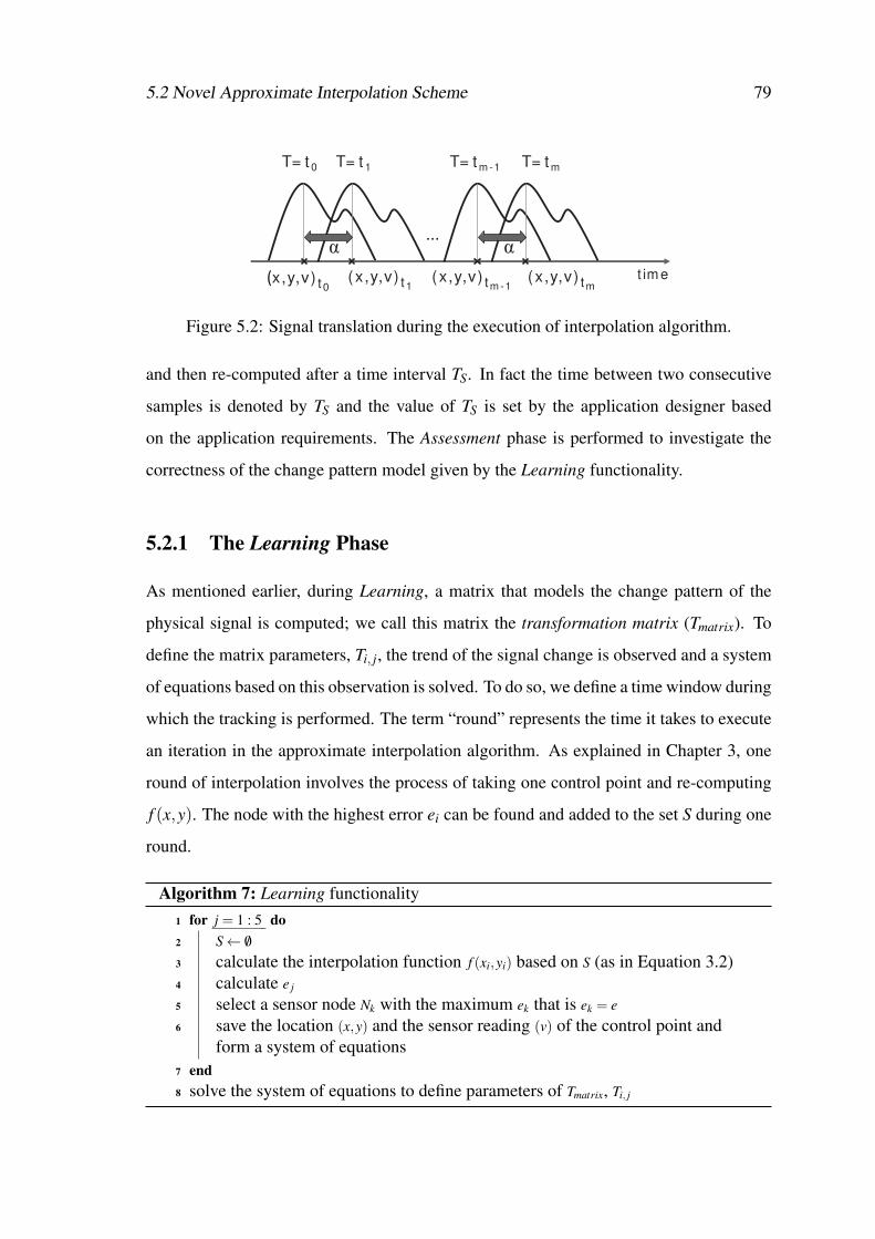
5.2 Novel Approximate Interpolation Scheme 79
T= t 0 T= t 1
(x,y,v) t0 (x,y,v) t1
T= tm -1
(x,y,v) tm -1
...
t im e
T= tm
(x,y,v) tm
α α
Figure 5.2: Signal translation during the execution of interpolation algorithm.
and then re-computed after a time interval TS. In fact the time between two consecutive
samples is denoted by TS and the value of TS is set by the application designer based
on the application requirements. The Assessment phase is performed to investigate the
correctness of the change pattern model given by the Learning functionality.
5.2.1 The Learning Phase
As mentioned earlier, during Learning, a matrix that models the change pattern of the
physical signal is computed; we call this matrix the transformation matrix (Tmatrix). To
define the matrix parameters, Ti, j, the trend of the signal change is observed and a system
of equations based on this observation is solved. To do so, we define a time window during
which the tracking is performed. The term “round” represents the time it takes to execute
an iteration in the approximate interpolation algorithm. As explained in Chapter 3, one
round of interpolation involves the process of taking one control point and re-computing
f (x,y). The node with the highest error ei can be found and added to the set S during one
round.
Algorithm 7: Learning functionality
1 for j = 1 : 5 do
2 S← /0
3 calculate the interpolation function f (xi,yi) based on S (as in Equation 3.2)4 calculate e j
5 select a sensor node Nk with the maximum ek that is ek = e
6 save the location (x,y) and the sensor reading (v) of the control point andform a system of equations
7 end
8 solve the system of equations to define parameters of Tmatrix, Ti, j

80 Self-Adaptive Approximate Interpolation scheme
Algorithm 7 summarizes the Learning functionality. It is assumed that there is a
monotonous change in a physical quantity, which implies that the overall shape of the
signal is preserved during the observation time. With this assumption, it can be claimed
that by nullifying the set S (Line 2 in Algorithm 7) at the beginning of each iteration,
it is possible to determine the location of the node with the highest error, which will
correspond to the peak in the observed physical signal. Figure 5.2 shows an example of a
dynamic signal that is translating with the rate of α in a specific direction. We found that
tracking the location of a specific point on the physical signal for five consecutive rounds
provides sufficient information to solve a system of equations through which the Tmatrix is
computed. We will justify this claim later, after explaining the procedure of updating set
S.
5.2.2 The Interpolation Phase
While performing the Interpolation, our algorithm uses the Tmatrix to update the data col-
lected in the previous iteration. In particular, the algorithm selects a new control point
at each round, and before computing the approximate interpolation f (x,y), all the previ-
ously selected points in set S update their three attributes (x,y,v) by applying the affine
transformation expressed by the Tmatrix (see Equation 5.1). xnewi, ynewi and vnewi are the
new (updated) versions of the x coordinate, the y coordinate and the value of the control
point pi in the current round.
xnewi← T1,1× xi +T1,2× yi +T1,3× vi +T1,4
ynewi← T2,1× xi +T2,2× yi +T2,3× vi +T2,4
vnewi← T3,1× xi +T3,2× yi +T3,3× vi +T3,4
(5.1)
5.2.3 Defining The Parameters of Tmatrix
One approach to define the model parameters, Ti, j : {i∈ {1,2,3}, j ∈ {1,2,3,4}} in Equa-
tion 5.1, is to observe the trend of signal dynamics and then solve a system of equations
based on that observation. To this end, as shown in Algorithm 7, we need to run the
interpolation algorithm consecutively five times just for one round. The reason is that
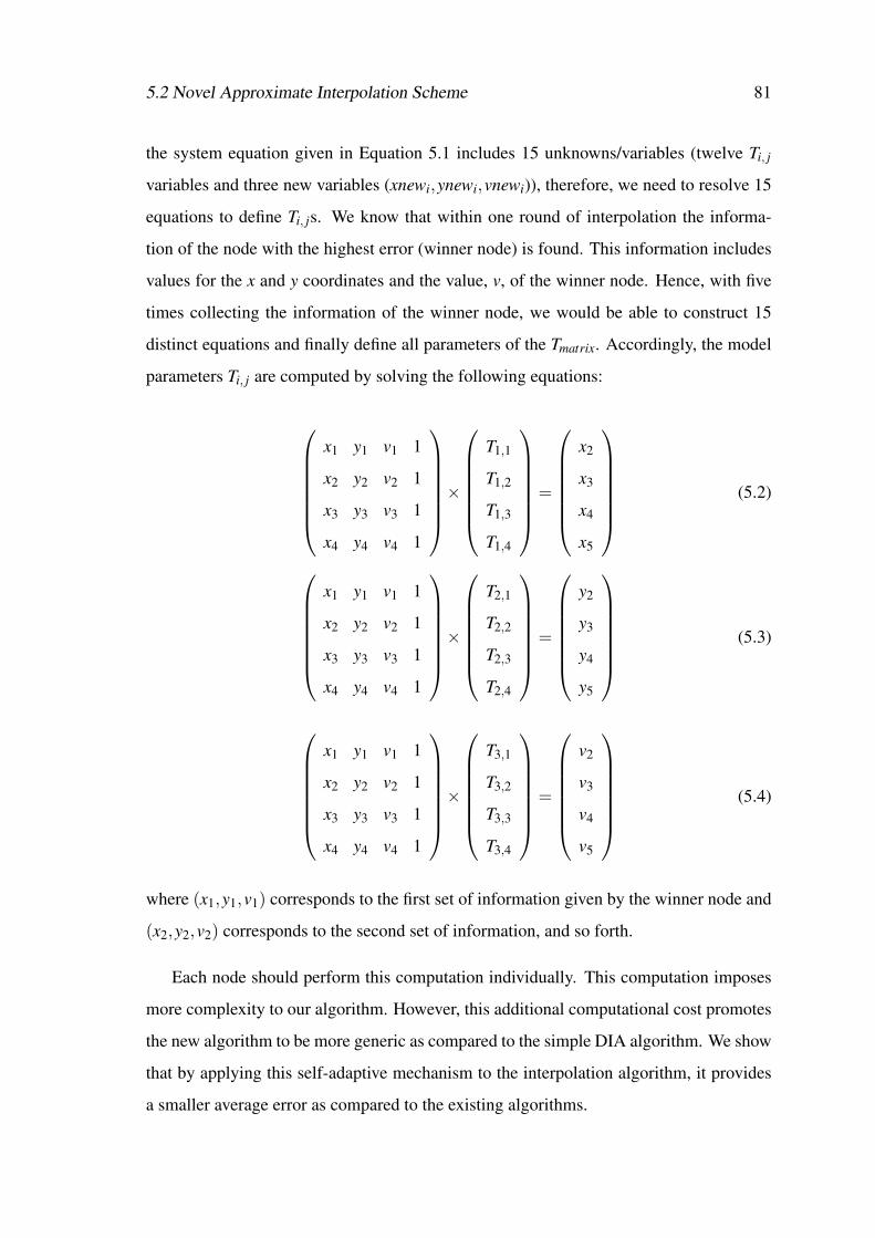
5.2 Novel Approximate Interpolation Scheme 81
the system equation given in Equation 5.1 includes 15 unknowns/variables (twelve Ti, j
variables and three new variables (xnewi,ynewi,vnewi)), therefore, we need to resolve 15
equations to define Ti, js. We know that within one round of interpolation the informa-
tion of the node with the highest error (winner node) is found. This information includes
values for the x and y coordinates and the value, v, of the winner node. Hence, with five
times collecting the information of the winner node, we would be able to construct 15
distinct equations and finally define all parameters of the Tmatrix. Accordingly, the model
parameters Ti, j are computed by solving the following equations:
x1 y1 v1 1
x2 y2 v2 1
x3 y3 v3 1
x4 y4 v4 1
×
T1,1
T1,2
T1,3
T1,4
=
x2
x3
x4
x5
(5.2)
x1 y1 v1 1
x2 y2 v2 1
x3 y3 v3 1
x4 y4 v4 1
×
T2,1
T2,2
T2,3
T2,4
=
y2
y3
y4
y5
(5.3)
x1 y1 v1 1
x2 y2 v2 1
x3 y3 v3 1
x4 y4 v4 1
×
T3,1
T3,2
T3,3
T3,4
=
v2
v3
v4
v5
(5.4)
where (x1,y1,v1) corresponds to the first set of information given by the winner node and
(x2,y2,v2) corresponds to the second set of information, and so forth.
Each node should perform this computation individually. This computation imposes
more complexity to our algorithm. However, this additional computational cost promotes
the new algorithm to be more generic as compared to the simple DIA algorithm. We show
that by applying this self-adaptive mechanism to the interpolation algorithm, it provides
a smaller average error as compared to the existing algorithms.

82 Self-Adaptive Approximate Interpolation scheme
5.2.4 The Assessment Phase
It is important to keep the model parameters up-to-date after computing the elements of
Tmatrix. The algorithm needs to be able to detect the occurrence of a sudden change in the
dynamics of the signal and adjust itself with the new change pattern. Applying feedback
from the sensor field is helpful. To do so, we use a subset of the control points, let’s say the
first ξ numbers taken into the previous sample, and broadcast their observed error value
as a feedback message to assess the quality of the Tmatrix. The observed error of a control
point is the difference between the measured value and the value of the interpolated signal
in its location. Therefore, the observed error computed during Assessment is used to
indicate the need for re-computing the transformation matrix. If the average observed
error is larger than a threshold value ε , the currently used parameters of Tmatrix are deemed
as not valid anymore, and Learning will execute. Algorithm 8 illustrates the Assessment
functionality.
Algorithm 8: Assessment functionality
1 Requirements:
2 (i) all nodes are aware of the start of the Assessment;3 (ii) latest set S is preserved: S = q1,q2, . . . ,qk;4 for j = 1 : ξ do
5 if id == qi.id then
6 compute the error and broadcast it7 else
8 wait to receive a packet and store the observed error value9 end
10 end
11 re-compute_Tmatrix← FALSE
12 if average observed error > ε then
13 re-compute_Tmatrix← T RUE
14 end
During Assessment, in order to collect feedback messages, we assume a TDMA-based
communication. The first requirement listed in Algorithm 8 is satisfied by utilizing the
same synchronization technique applied to the prioritized MAC protocol [Bos91, PAT07,
PGAT09], since all nodes agree on a common reference time to start either a round of
interpolation or a TDMA-slot.

5.3 Algorithm Evaluation 83
The Assessment functionality is performed with a periodicity TA that is a multiple
of TS. The exact value of the self-assessment periodicity is defined by the application
designer according to the required accuracy level. Intuitively, the smaller the Assessment
frequency, the more accurate representation of the signal will be achieved.
5.3 Algorithm Evaluation
To evaluate the self-adaptive interpolation scheme, we developed several simulations in
MATLAB, first to assess the efficiency of the transformation matrix, Tmatrix, in computing
only one sample of the physical signal and compare it against the basic approach. Then
we examined the execution of the self-adaptive approach in an application simulated by
MATLAB, where we aim at performing a continuous monitoring of a signal with a given
pattern change.
5.3.1 The Efficiency of Tmatrix
As discussed in Chapter 3, the approximate representation of the physical signal can be
obtained by executing the interpolation algorithm for a number of rounds (defined by k in
Algorithm 1). Through extensive simulations, we studied the average error of a sample of
a physical signal computed by the basic interpolation approach and the new self-adaptive
approach. We consider a dense network with 2500 nodes, deployed in a square grid
fashion. We also consider having an input physical signal that can be modeled by a single
peak middle shape signal (similar to the one given in Figure 3.1(a)) with the following
Gaussian function:
p(x,y) = e−7((x−0.5)2+(y−0.5)2)+0.1 (5.5)
Three types of linear signal changes are considered : (i) scaling, (ii) increment and
(iii) translation. Figure 5.3 compares the average error of a sample computed by the BIA
and the self-adaptive algorithm as a function of the number of considered interpolation
rounds. Simulation results show a remarkable improvement in the average error of a
sample computed by the novel self-adaptive approach independently of the considered

84 Self-Adaptive Approximate Interpolation scheme
30
40
50
60
70
Error(%
) BIA
Self‐adaptive
0
10
20
30
7 10 15 20 30 50
Average
Round
20
25
30
35
40
45
eError(%
) BIASelf‐adaptive
0
5
10
15
7 10 15 20 30 50
Average
Round
40
50
60
70
80
eError
(%) BIA
Self‐adaptive
0
10
20
30
7 10 15 20 30 50
Average
Round
(a) Scale (10%) (b) Increment (10%) (c) Translate (2%)
Figure 5.3: Average error in a sample computed by the BIA and the novel self-adaptiveapproach.
signal change model. While the novel approach provides a fair estimation of the physical
signal (with an average error of about 3%), the BIA presents much poorer results. The
average error of a sample computed by BIA keeps rising when the number of interpolation
rounds increases. The reason is that dislike the self-adaptive approach that updates the
value of the previously selected control points qi in the set S before computing the f (x,y),
in the BIA approach, the value of the selected control points in S remains unchanged. This
leads to a major deviation between the computed approximate interpolation and the real
physical signal. In fact, longer execution of the interpolation deteriorates the accuracy of
the sample computed by the BIA approach.
5.3.2 Performance Evaluation of Self-Adaptive Scheme
We consider the same simulation set up as in the previous subsection and the same input
signal as defined by the Equation (5.5). The aim of this set of simulations is to assess the
self-adaptive approach for the “continues” monitoring of a dynamic signal. In the exper-
iments, we consider abrupt change patterns in the signal, applied by the displacement of
the whole signal up and down. We express the displacement in terms of relative speed as
compared to the duration of a round.
Figure 5.4 shows the speed of the change during the simulation time (4000 rounds).
The positive values and negative values represent “movements” up and down, respec-
tively. Note that the values change equally in all points (xi,yi) of the grid.
We run the simulation for 4000 rounds and set TS to 25 rounds and TA to 3×TS, which
means that a new sample is computed every 25 rounds and the Assessment runs every

5.3 Algorithm Evaluation 85
0 500 1000 1500 2000 2500 3000 3500 4000-8
-6
-4
-2
0
2
4
6
8
10
12
14
16
18
Round
Sig
nal C
han
ge R
ate
(%
per
tim
e-s
lot)
(a) Change pattern scenario.
0 500 1000 1500 2000 2500 3000 3500 40000
5
10
15
20
25
30
Round
Avera
ge E
rro
r (%
)
(b) The BIA approach.
0 500 1000 1500 2000 2500 3000 3500 40000
5
10
15
20
25
30
Round
Avera
ge E
rro
r (%
)
(c) The self-adaptive approach.
Figure 5.4: The average error of samples computed by the BIA and the self-adaptiveapproaches with TS = 25 rounds and TA = 3×TS.
75 rounds. The number of control points is set to 6, which indicates that a new sample
is computed during 6 rounds. In Assessment, we chose the first five control points that

86 Self-Adaptive Approximate Interpolation scheme
Time-Slot Number
0 20 40 60 80 100 120 140 160 180 200 220 240
Av
era
ge
Err
or
(%)
0
5
10
Figure 5.5: The zoom in view of the average error of samples computed by self-adaptiveapproach with TS = 25 rounds and TA = 3×TS.
contributed in computing the latest interpolation sample (ξ = 5).
Since we set TA to 3×TS, in the worst case, we may observe three samples with lower
quality. In our described scenario, this happens for instance after round 100, when the
change rate increases from 12% to 14%. Figure 5.5 shows the zoom-in view of Fig-
ure 5.4(c). Since the last assessment has occurred at round 86, and the next assessment
occurs at round 161 (75 rounds later), the samples taken in rounds 111, 136 and 161 are
computed with an outdated Tmatrix, hence we see three low quality samples in a row. After
the assessment in round 167, since the average observed error is not small enough (ε is
chosen 0.01), all nodes prepare to execute the Learning phase to recompute the Tmatrix.
The self-adaptive approach provides more accurate results (average error of about 3%)
as compared to the BIA approach. For the simple physical signal with low change rate,
the performance of the BIA approach is roughly the same as that of our novel algorithm,
but for more complex signals, where there is a need to have more points in the set S for
computing one sample, the novel algorithm outperforms BIA, even for slow change rates.
Besides, in worst case and for the described experiment, the novel algorithm provides
samples with 9% as the largest average error, while with BIA, samples with an average
error of 27% may result, especially when the signal change rate is high.
5.4 Summary 87
5.4 Summary
In Chapter 3, we described how the BIA approach enables to efficiently compute an ap-
proximate interpolation of a physical signal. The BIA approach works well for the case
where a smooth physical signal is monitored and with the assumption that the signal re-
mains steady over the time it takes to obtain an approximate sample. The DIA algorithm
is also described as an attempt to provide a more accurate interpolation by embedding
the physical dynamics into the interpolation algorithm. However, the DIA is unable to
provide a system-dependent interpolation algorithm, since the proper change pattern pa-
rameters cannot be detected at run-time; they must be defined a-priori by the application
designer. This chapter discussed and described a solution to tackle the above mentioned
problem. Our novel algorithm provides an accurate approximate interpolation even if the
signal and change patterns alter during the execution of the interpolation algorithm. More
importantly, the algorithm self-adapts to incorporate variations in the change pattern.
Possible future work would involve synthesizing such an algorithm from a model of
the physical world by incorporating changes in the Assessment rate as part of the feedback
control as well as a more sophisticated technique to model more complex change patterns
(not monotonous in the area of observation).

88 Self-Adaptive Approximate Interpolation scheme

Chapter 6
Feature Extraction in Densely Sensed
Environments
In this chapter, we present a novel feature extraction mechanism for dense sensor net-
works, where all nodes are located in one single broadcast domain (SBD). Then, we
extend our SBD algorithm for a large dense network with multiple broadcast domains
(MBD), where all nodes may not reside within the communication range of each other.
This feature extraction mechanism employs the prioritized channel access mechanism of
dominance-based protocols (i) to efficiently obtain global extrema of sensed quantities,
(ii) to extract local extrema and (iii) to detect boundaries of events.
6.1 Feature Extraction
With the reduction in size and cost of sensor nodes, dense sensor networks are becoming
more popular in a wide-range of applications. Some of these applications aim at pro-
viding an approximate interpolation of the monitored physical quantities, as discussed in
Chapter 5. Some other applications with dense deployments are geared towards finding
various patterns or features in the spread of sensed physical quantities over an area. In
this Thesis, we define feature extraction as the process of determining certain features
such as peaks, boundaries and shapes in the distribution of a physical quantity. Based on
89
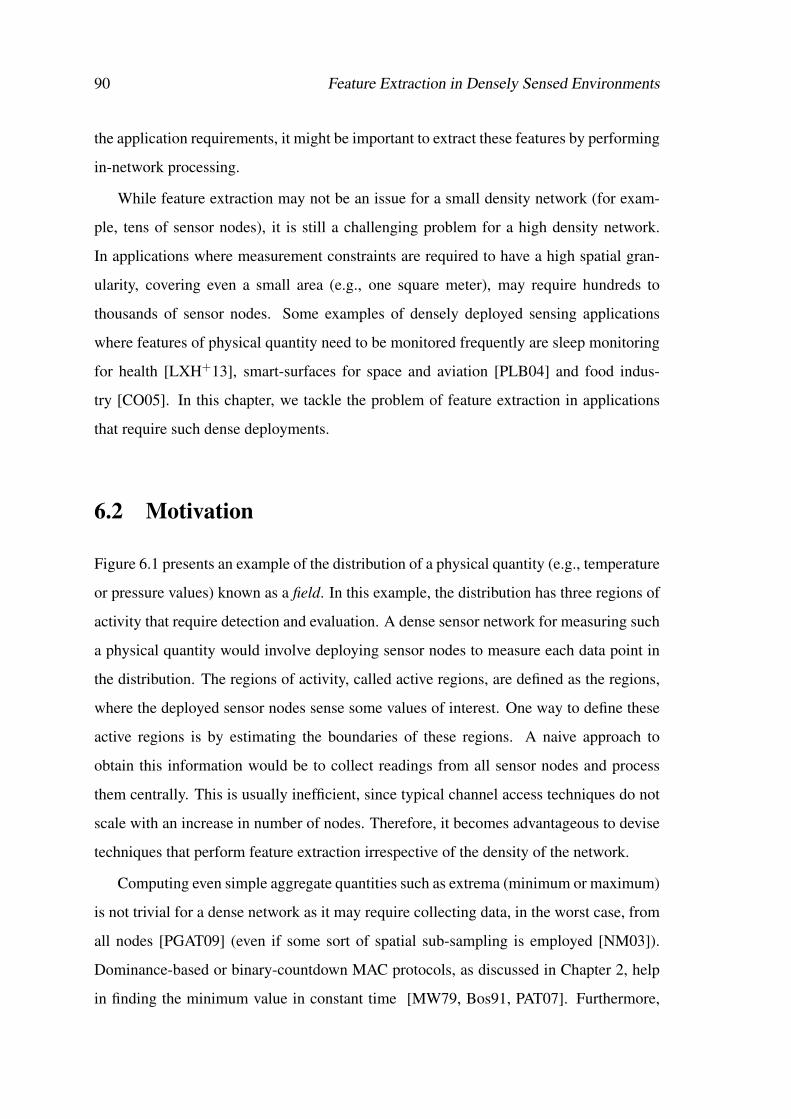
90 Feature Extraction in Densely Sensed Environments
the application requirements, it might be important to extract these features by performing
in-network processing.
While feature extraction may not be an issue for a small density network (for exam-
ple, tens of sensor nodes), it is still a challenging problem for a high density network.
In applications where measurement constraints are required to have a high spatial gran-
ularity, covering even a small area (e.g., one square meter), may require hundreds to
thousands of sensor nodes. Some examples of densely deployed sensing applications
where features of physical quantity need to be monitored frequently are sleep monitoring
for health [LXH+13], smart-surfaces for space and aviation [PLB04] and food indus-
try [CO05]. In this chapter, we tackle the problem of feature extraction in applications
that require such dense deployments.
6.2 Motivation
Figure 6.1 presents an example of the distribution of a physical quantity (e.g., temperature
or pressure values) known as a field. In this example, the distribution has three regions of
activity that require detection and evaluation. A dense sensor network for measuring such
a physical quantity would involve deploying sensor nodes to measure each data point in
the distribution. The regions of activity, called active regions, are defined as the regions,
where the deployed sensor nodes sense some values of interest. One way to define these
active regions is by estimating the boundaries of these regions. A naive approach to
obtain this information would be to collect readings from all sensor nodes and process
them centrally. This is usually inefficient, since typical channel access techniques do not
scale with an increase in number of nodes. Therefore, it becomes advantageous to devise
techniques that perform feature extraction irrespective of the density of the network.
Computing even simple aggregate quantities such as extrema (minimum or maximum)
is not trivial for a dense network as it may require collecting data, in the worst case, from
all nodes [PGAT09] (even if some sort of spatial sub-sampling is employed [NM03]).
Dominance-based or binary-countdown MAC protocols, as discussed in Chapter 2, help
in finding the minimum value in constant time [MW79, Bos91, PAT07]. Furthermore,
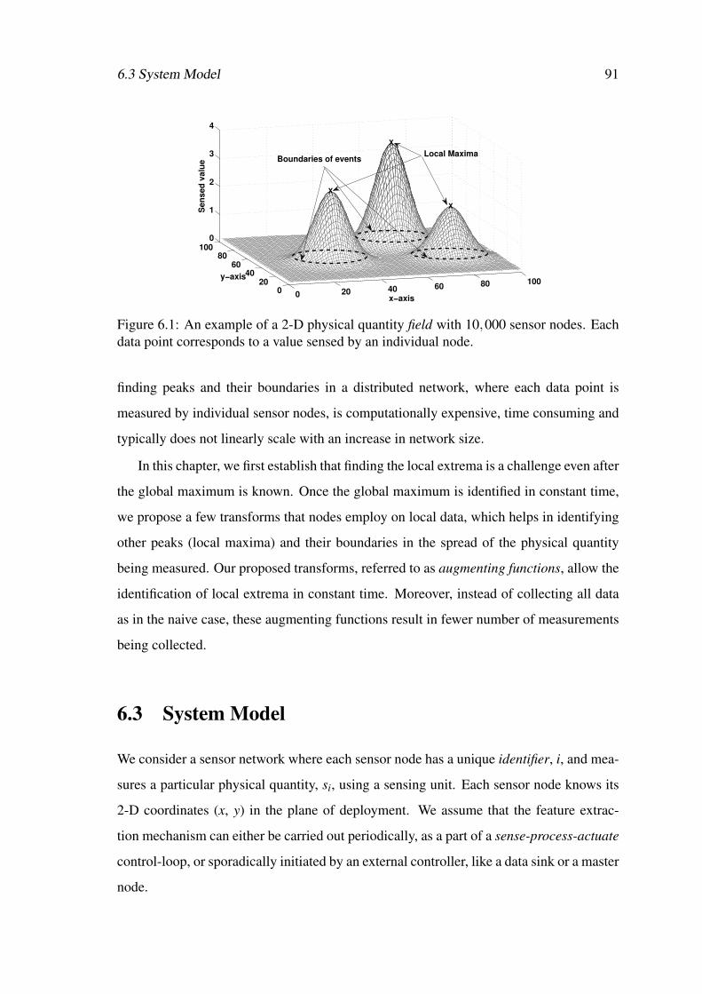
6.3 System Model 91
0 20 40 60 80 1000
2040
6080
1000
1
2
3
4
x−axis
y−axis
Se
ns
ed
va
lue
X
X
X
Boundaries of eventsLocal Maxima
Figure 6.1: An example of a 2-D physical quantity field with 10,000 sensor nodes. Eachdata point corresponds to a value sensed by an individual node.
finding peaks and their boundaries in a distributed network, where each data point is
measured by individual sensor nodes, is computationally expensive, time consuming and
typically does not linearly scale with an increase in network size.
In this chapter, we first establish that finding the local extrema is a challenge even after
the global maximum is known. Once the global maximum is identified in constant time,
we propose a few transforms that nodes employ on local data, which helps in identifying
other peaks (local maxima) and their boundaries in the spread of the physical quantity
being measured. Our proposed transforms, referred to as augmenting functions, allow the
identification of local extrema in constant time. Moreover, instead of collecting all data
as in the naive case, these augmenting functions result in fewer number of measurements
being collected.
6.3 System Model
We consider a sensor network where each sensor node has a unique identifier, i, and mea-
sures a particular physical quantity, si, using a sensing unit. Each sensor node knows its
2-D coordinates (x, y) in the plane of deployment. We assume that the feature extrac-
tion mechanism can either be carried out periodically, as a part of a sense-process-actuate
control-loop, or sporadically initiated by an external controller, like a data sink or a master
node.

92 Feature Extraction in Densely Sensed Environments
As stated earlier in this chapter, the collection of all sensor values across the total
sensed area is referred to as a field (shown in Figure 6.1). Each data point in the field
corresponds to a true (or non-faulty) sensor reading value, sensed by an individual sensor
node at its physical location. The spatial granularity and the size of the field is directly
correlated to the distribution of the nodes and their spread. We also define active region
as a physical area populated by sensor nodes that sense some activity. The overarching
goal of our technique is to find location, boundaries and shape of an active region, which
we referred to as features, in the physical environment. To illustrate and evaluate our
approach, we generate various sample fields by a summation of 2-D Gaussian functions.
Function M (vi) represents the process of finding the MIN over values vi published
by independent sensor nodes in a broadcast medium, where i ∈ {1,2, ...N} and N is the
number of sensor nodes in a broadcast domain. In fact, M (vi) represents one execu-
tion of interpolation round, as discussed in Chapter 5, for an SBD domain (later on, in
Section 6.5.2 we will discuss the details of function M for MBD, where several num-
ber of rounds need to be run). We exploit the property of simultaneous transmissions in
dominance-based protocols to devise this function. vi is the scaled value that each sensor
node computes based on its measured value si and the global maximum smax measured in
the field.
After each round, all the other sensor nodes know the identifier and the location of the
sensor node with the MIN value. This sensor node is known as the winner of the round.
We use i to denote the identifier of the winner. Hence, the function M can be formally
represented as:
{v, i, x, y}= M (vi) ∀i ∈ {1,2, ...N}
where x and y are the x and y coordinates of the sensor node with the global minimum
value v.
The choice of the vi values used by an ith sensor node in the application of function
M depends on the requirements of the application. It should be noted that a sensor
node can only use its local information (such as identifier, sensor value and physical
location) and other global data available from the previous iterations of M . For our goal
of identifying various features, we augment (or transform) these input values such that the

6.4 Feature Extraction Using Augmenting Functions 93
Table 6.1: Summary of the symbols and notations used in this chapter.
Symbol Description
si sensor value measured by sensor node i
smax maximum value collected by sensor nodes
νi =1+si
smaxscaled sensor value with respect to the maximum value over all sensornodes
Aβ , Aγ , Aδ augmenting functions used for different feature extraction techniquesM (vi) finding the MIN over all vi valuesM (−vi) finding the MAX over all vi valuesφ(νi,xi,yi) function computed by sensor nodesπs termination condition
global minimum returned by M corresponds to one of the local minima or an edge of an
active region.
The function M can be applied to the value computed by φi, which is a function of the
sensor values and their location. The codomain of the function φi denotes a set of values
it can take. We assume that the cardinality of the codomain of φi is large enough that the
probability of computing the same φi by two sensor nodes is negligible and thus an unique
sensor node i is chosen. The time-complexity of M is proportional to the number of bits
used to encode φi, and hence, it is proportional to the logarithm of the cardinality of the
codomain. However, as all sensor nodes transmit simultaneously in a dominance-based
MAC protocol, the time required for the application of M over a network is independent
of the number of sensor nodes. Table 6.1 summarizes the notations and symbols that
we use in the following sections, where we define a set of functions to extract different
features of the field.
6.4 Feature Extraction Using Augmenting Functions
In this section, we describe in detail a set of augmenting functions that can extract an
approximate but faithful representation of various features in the field by applying simple
transforms on the sensor values. We show that this process can be done with a limited
number of broadcast messages or floodings in the cases of SBD or MBD, respectively.
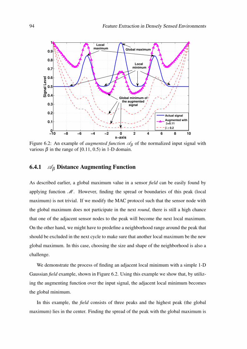
94 Feature Extraction in Densely Sensed Environments
−10 −8 −6 −4 −2 0 2 4 6 8 100
0.1
0.2
0.3
0.4
0.5
0.6
0.7
0.8
0.9
1
x−axis
Sig
na
l L
ev
el
Actual signal
Augmented with β=0.11
β ≥ 0.2
Global maximum
Local maximum
Global minimum ofthe augmented
signal
Local minimum
Figure 6.2: An example of augmented function Aβ of the normalized input signal withvarious β in the range of [0.11, 0.5) in 1-D domain.
6.4.1 Aβ Distance Augmenting Function
As described earlier, a global maximum value in a sensor field can be easily found by
applying function M . However, finding the spread or boundaries of this peak (local
maximum) is not trivial. If we modify the MAC protocol such that the sensor node with
the global maximum does not participate in the next round, there is still a high chance
that one of the adjacent sensor nodes to the peak will become the next local maximum.
On the other hand, we might have to predefine a neighborhood range around the peak that
should be excluded in the next cycle to make sure that another local maximum be the new
global maximum. In this case, choosing the size and shape of the neighborhood is also a
challenge.
We demonstrate the process of finding an adjacent local minimum with a simple 1-D
Gaussian field example, shown in Figure 6.2. Using this example we show that, by utiliz-
ing the augmenting function over the input signal, the adjacent local minimum becomes
the global minimum.
In this example, the field consists of three peaks and the highest peak (the global
maximum) lies in the center. Finding the spread of the peak with the global maximum is

6.4 Feature Extraction Using Augmenting Functions 95
not trivial as the global minimum point can be one of those sensor nodes near the borders
of the field. It is important to suitably modify the process of identifying the extrema such
that a local minimum adjacent to a peak (adjacent valley) can be found. For this purpose,
we observe that an adjacent valley should have a low value and its distance from the peak
should also be small. Hence, each value in the field is transformed (multiplied) with the
distance from the peak. With this transformation, the points located farther from the peak
are associated with higher values (compared with its sensed value) and only points with
the lowest sensed value and the smallest distance from the peak can become the global
minimum in the augmented field. It is possible that this global minimum is a point in an
adjacent valley. The boundary of this peak is found with just two rounds of executing
M function: (i) finding the global maximum in the original field; and (ii) identifying the
global minimum in the augmented field.
For 2-D Gaussian fields, the 1-D approach described above can be directly applied.
Different active regions of the field are found by excluding the sensor nodes lying inside
the identified active region from participating in the next rounds. The process of finding
active regions is shown in Algorithm 9. Initially, function M is used to find the global
maximum (smax), then a circular area around the identified peak is filtered out. The radius
of this filtering circle is set as the distance of an adjacent valley from the peak. The
value and the location of the adjacent valley (Sad j−valley and dad j−valley) are found by one
application of M function (line 9 in Algorithm 9).
Each sensor node uses a function φβ as an input to M . The function φβ takes into
account two properties of the field: (i) sensed value s; and (ii) sensor’s proximity to the
peak d. That function is defined as follows:
φβ = ν×Aβ (d) (6.1)
ν is the scaled value and is defined as:
ν =1+ s
1+ smax(6.2)
and smax is the value of the global maximum, found at the beginning of the algorithm.

96 Feature Extraction in Densely Sensed Environments
Algorithm 9: Distance augmenting function (Aβ ) executed on each sensor node ni
1 begin
2 Silent← 03 smax←M (−φs) // find global MAX
4 πs← a fraction of smax // termination condition setting
5 while snew−peak > πs do
6 if Silent 6= 1 then // if the node is not filtered out
7 snew−peak←M (−φs) // find the new peak
8 compute φ based on Equation 6.19 < sad j−valley,dad j−valley >←M (φβ )
10 R f ← dad j−valley
11 di← distance between new-peak and node ni
12 if di < R f then
13 Silent← 114 end
15 end
16 end
17 end
Aβ (d) is the augmenting function, which is formulated as follows:
Aβ (d) = eβ ( d
dmax)2
(6.3)
where dmax is the diameter of the monitored area, and it is used to normalize the distance
from the peak. β is a parameter to control the impact of distance on the augmented field
with respect to the scaled value ν . To ensure that the winning sensor node is located at
the adjacent local minimum of the field, the priority function φβ is computed so that the
distance is exponentially penalized.
Finally, by finding the global minimum over φβ values at all the sensor nodes, we are
able to find a point that lies in the adjacent valley with a high probability. The distance
between the adjacent valley point and the peak determines the filtering radius, R f (line 10
in Algorithm 9). Sensor nodes that are located within the filtering circle refrain from
participating in the next iterations. Repeating this procedure conducts to finding all the
peaks in the region. The algorithm stops when the value of the new peak (snew−peak) is
lower than a certain user defined threshold πs, which is a fraction of the global maximum.
By finding the peaks and their spread, this approach helps in identifying the location and
the number of circular active regions in a field.

6.4 Feature Extraction Using Augmenting Functions 97
6.4.2 Aγ Vector Augmenting Function
Our second augmenting function is used for cases where we are interested in finding a
boundary around all active regions. This approach can be used for a range of applications
such as crowd monitoring for smart cities or sleep monitoring for health-care. In this
approach, if we assign larger values of φ to sensor nodes that lie on the boundary of an
active region, then the result of applying the M function over the negation of the φ value
corresponds to the boundary of active regions. This is implemented by augmenting the
sensor values with a function that grows in a particular direction.
The vector augmenting function Aγ is designed to work with binary fields, where the
input signal is not smoothly distributed, and two neighboring sensor nodes may have very
close or very different measurements. By applying Aγ , each sensor node multiplies its
measurement with a vector ~u. The rationale behind using a direction is to find the sensor
nodes that sense a high value and are located as far as possible in the direction given by
~u, which corresponds to the edge of an active region in that direction. To compute the
function φ , sensor nodes transform their locations with a direction as follows:
φγ = vp×Aγ(x,y,θ) (6.4)
where vp is a participation value, which is either 0 or 1, depending on the sensed value
being below or above a threshold. Sensor nodes with vp = 1 are part of the active region.
The augmenting function is defined as follows:
Aγ(x,y,θ) = eγ(x.cos(θ)+y.sin(θ)) (6.5)
x and y are the coordinates of the sensor location and θ is the direction given by vector~u.
By using Aγ , the value is “projected” in a direction given by the vector~u. The sensor
node that has the largest value has a high probability of being located on the border of an
active region in the direction of~u.
The way this approach works is outlined in Algorithm 10. The algorithm explores
the region by choosing random directions defined in a set {vθ}. We assume that the seed
for generating this pseudo-random directions is generated by the initiator of the boundary

98 Feature Extraction in Densely Sensed Environments
Algorithm 10: Vector augmenting function Aγ , executed on each sensor node ni
1 begin
2 smax←M (−φs) // find global MAX
3 πs← a fraction of smax // termination condition setting
4 { fθ}←∅ // the set of filtered directions
5 if s < πs then
6 vp← 17 else
8 vp← 09 end
10 {vθ}← a set of θ directions11 foreach θ ∈ {vθ} do
12 if θ /∈ { fθ} then
13 compute φγ based on Equation 6.414 < sedge,(x,y)edge,θedge >←M (−φγ)
15 if (x,y)edge was found with other direction θx then
16 { fθ}← { fθ}∪θxθ +2ε
17 end
18 end
19 end
20 end
detection process. Thus, all the sensor nodes will use the same {vθ} in each iteration.
Repeating this procedure in different directions makes it possible to find the boundary of
an active region by computing the convex hull of the collected locations.
If two angles lead to a same point, it means that any angle over the arc confined
by these two angles would result in that point. Thus, this arc can be filtered out from
further investigation. Figure 6.3 shows an example where two angles of θ1 = 31◦ and
θ2 = 89◦ lead to find the same location P2. In this case, there is no need to examine more
directions in the region of 31◦ ≤ θ ≤ 89◦. We also use marginal extension ε to limit
further the redundant directions in the arc denoted by θi± ε . We discuss the impact of ε
in Section 6.6.
More iterations of the algorithm leads to more accurate boundaries, but at the cost
of more resource consumption. We show in Section 6.6 that with the above filtering
strategy, we are able to reduce the number of dominance rounds, while still building a
valid description of the active region. The worst case for our algorithm happens when the
event boundary looks like a perfect circle where each new direction will give a new point
(assume having a very dense deployment of sensors and consider a marginal extension of
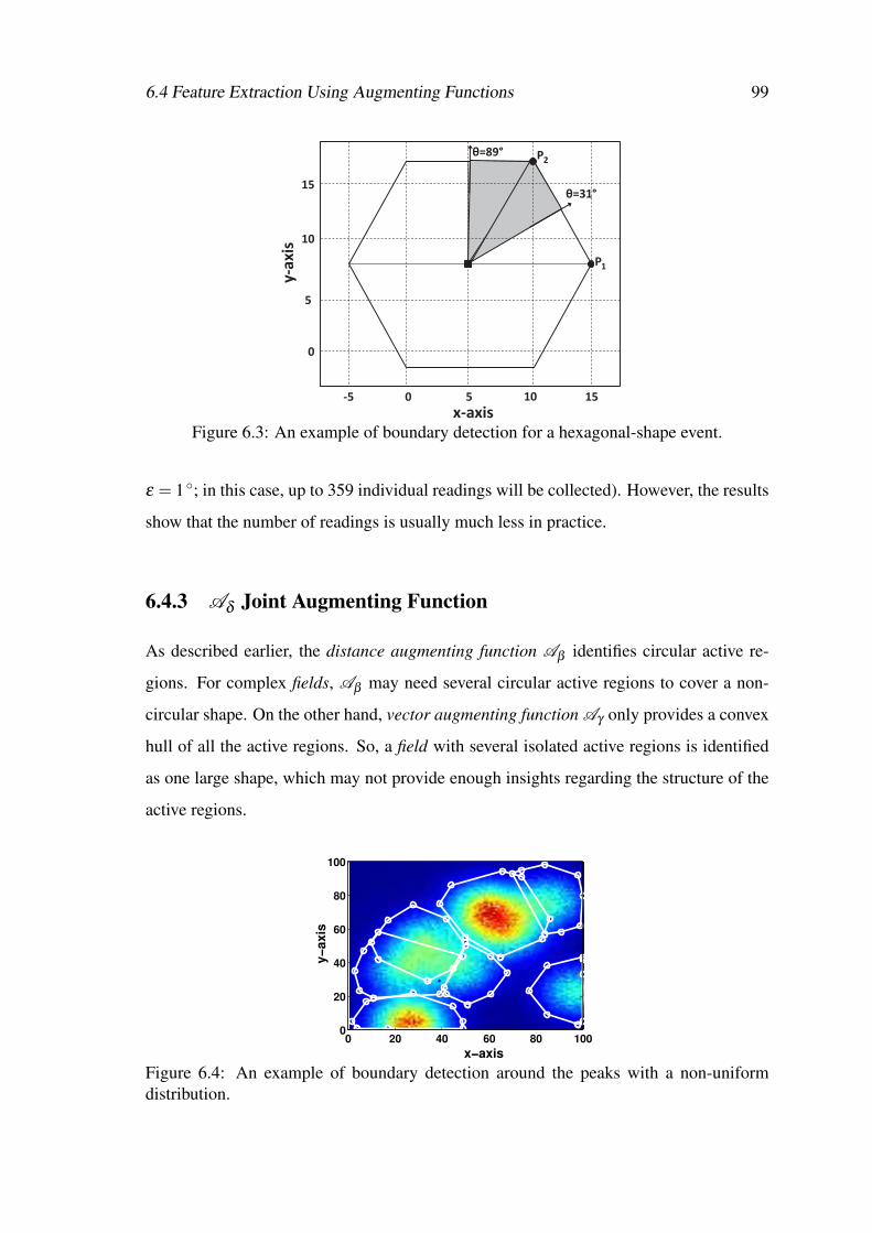
6.4 Feature Extraction Using Augmenting Functions 99
=89°
15
10
5
0
-5 0 5 10 15
P
P
x-axis
y-axis
2
1
=31°
Figure 6.3: An example of boundary detection for a hexagonal-shape event.
ε = 1◦; in this case, up to 359 individual readings will be collected). However, the results
show that the number of readings is usually much less in practice.
6.4.3 Aδ Joint Augmenting Function
As described earlier, the distance augmenting function Aβ identifies circular active re-
gions. For complex fields, Aβ may need several circular active regions to cover a non-
circular shape. On the other hand, vector augmenting function Aγ only provides a convex
hull of all the active regions. So, a field with several isolated active regions is identified
as one large shape, which may not provide enough insights regarding the structure of the
active regions.
x−axis
y−axis
0 20 40 60 80 1000
20
40
60
80
100
Figure 6.4: An example of boundary detection around the peaks with a non-uniformdistribution.

100 Feature Extraction in Densely Sensed Environments
To find the boundary of an active region with a non-circular distribution, we devised
a new augmenting function Aδ , that is a composition of Aβ and Aγ . By applying Aδ ,
sensor nodes that were identified with the M function should have the following proper-
ties: (i) lie close to the peak; and (ii) locate on the edge of the local boundary in a given
direction. The value used by each sensor node is then defined as follows:
φδ = Aδ ×Aβ (d)
Aγ(x,y,θ)(6.6)
where Aδ is given by:Aδ = ν−δ
Aδ is an inverse polynomial of degree δ of the scaled sensed value ν , and δ is a parameter
to guarantee that the low values lying far away from a peak bring a stronger contribution
to the φ values. As a consequence, for a given value of θ , the point that has the minimum
value of φδ is more likely to lie on the boundary in the θ direction. We sweep the area
around a peak with different values of θ . In our evaluation, for θ , we used equal intervals
of π/4 (θ ∈ {0,π/4, ...2π}). Smaller intervals will result in better accuracy of boundary
at the cost of higher number of broadcast messages. Thus, after finding a new peak, the
locations of the nearest adjacent valleys in eight directions are found, and the convex hull
of all these readings represents the area around that active region. This enables us to find
complex geometric shapes according to the shape of active regions instead of only circles,
as shown with an example in Figure 6.4.
6.5 Computing Global Extrema in MBD Networks
In this section, we address the challenge of computing MIN in a dense network, where
nodes are not necessarily confined to an SBD. We consider two different approaches to ex-
tend the functionality of M function for MBD dense networks: (i) clustering the network
into several SBDs as proposed in [APT07], and (ii) a novel approach using concurrent
transmissions by taking advantage of the dominance-based protocol.

6.5 Computing Global Extrema in MBD Networks 101
Leader node
Cluster leader
Sensor node
Cluster borders
Balck-node tree
T1=1
T2=2 T
3=5
T4=3
T6=4
T5=6 T
7=2
T8=4
T9=5
T10
=1 T
17=2
T16
=2
T12
=4
4 T14
=3 T
T11
=5
T18
=1
T15
=1
T13
=3
(a) (b) (c)
Figure 6.5: Cluster-based approach: (a) cluster formation and black-node tree (B) con-struction. Rco = 5 and we assume r = Rco/2. With the given virtual range r, 18 clustersare constructed; (b) cluster interfering graph Gi (with d = 14). This graph is used by theleader node to compute the activation timeslot for each cluster. Two clusters are assumedto be interfering if the distance between the cluster leaders is less than 3× r; (c) timeslotassignments (the chromatic number for the interfering graph is 6).
6.5.1 The Cluster-based Approach
In the clustering approach, proposed in [APT07], a topology discovery algorithm is first
executed to partition the network such that all nodes in each partition are in the same
broadcast domain (Setup phase). Then, at runtime, nodes within the same cluster find
the minimum sensor reading and communicate these values to their cluster leaders. The
cluster leaders form a collection tree with root at the leader node where the query for
computing MIN was initiated.
The high-level pseudo code of the cluster-based approach is given in Algorithm 11.
A minimum virtual dominating set (MVDS), as introduced in [DBN03], has been consid-
ered during the setup phase. With MVDS it is possible to divide the network into several
clusters where the nodes in each cluster form an SBD domain. The cluster leaders (known
as black-nodes in MVDS) are responsible for collecting MIN in each cluster and forward-
ing it to the leader node through a collection tree graph known as black-node tree (B).
The virtual range is used to guarantee that all nodes in a cluster are located in the same
broadcast domain. In fact the MVDS is a distributed algorithm with two main phases.
In the propagation phase, it forms the clusters; and in the response phase, the topology
information is delivered to the leader node (the node initiating the aggregation query).
Figure 6.5-(a) shows an example of cluster construction using MVDS.
The leader node uses this topology information to schedule the activation time of

102 Feature Extraction in Densely Sensed Environments
Algorithm 11: Cluster-based approach
1 begin
2 run MVDS(Rco,r) [DBN03] to partition the network (setup phase) // execute on
each sensor node ni
3 construct cluster interfering graph Gi(V,E) and black-node tree B (responsephase) // execute on leader node
4 ∆← timeslot-assignment(G) // executed on leader node
5 for i = 1 to ∆ do
6 execute one dominance round according to assigned timeslot // execute on
nodes in each active cluster
7 end
8 collect data from black-node tree B // execute on leader node
9 disseminate global MIN to the network // execute on leader node
10 end
each cluster to avoid any collision between neighboring nodes that reside in different
clusters. To make this approach more efficient, we utilize a heuristic that was proposed
for the register interfering graph (RIG) problem [KP87] to find the chromatic number ∆
for concurrent active clusters. However, unlike the RIG problem, in our case the number
of available colors is not known in advance. k is the number of registers in the RIG
problem.
Function timeslot-assignment(G) is performed by the leader node to find the
value of ∆ as shown in Algorithm 12. From basic graph theory it is known that, for an n-
node graph G(Vn,E), if the maximum degree of nodes in the graph is d, then it is possible
to color the graph with d+1 different colors [JT11]. In our modified heuristic, the leader
node initiates the process of finding ∆ by setting k to ⌈d+12 ⌉, and then restricts the search
area [kmin,kmax]. If the current k is able to color the graph (line 6 in Algorithm 12), the
algorithm will add k into the set of possible chromatic numbers {C} and updates kmax,
otherwise, it updates kmin. The algorithm terminates when the current k is larger than an
element in the set {C}. For the example given in Figure 6.5, with d = 14, the algorithm
finds ∆ = 6 after four assignments of k.
6.5.2 The Ripple-based Approach
The ripple-based approach aims at eliminating the setup overhead in the cluster-based ap-
proach and mitigating the initialization cost by using a distributed algorithm to compute

6.5 Computing Global Extrema in MBD Networks 103
Inactive sensor node
Active sensor node
Initiative sensor node
Communication range
Ripple border
(a)
v
(b) (c)
(d) (e)
Figure 6.6: Ripple propagation throughout the network: (a) an initiator sensor node thatsignals start of a tournament. Sensor nodes within the communication range of this nodethen perform one tournament; (b) nodes participating in the previous tournament becomeinitiator nodes in this round; (c) and (d) ripple moves toward the border of the network;and (e) all sensor nodes are activated.
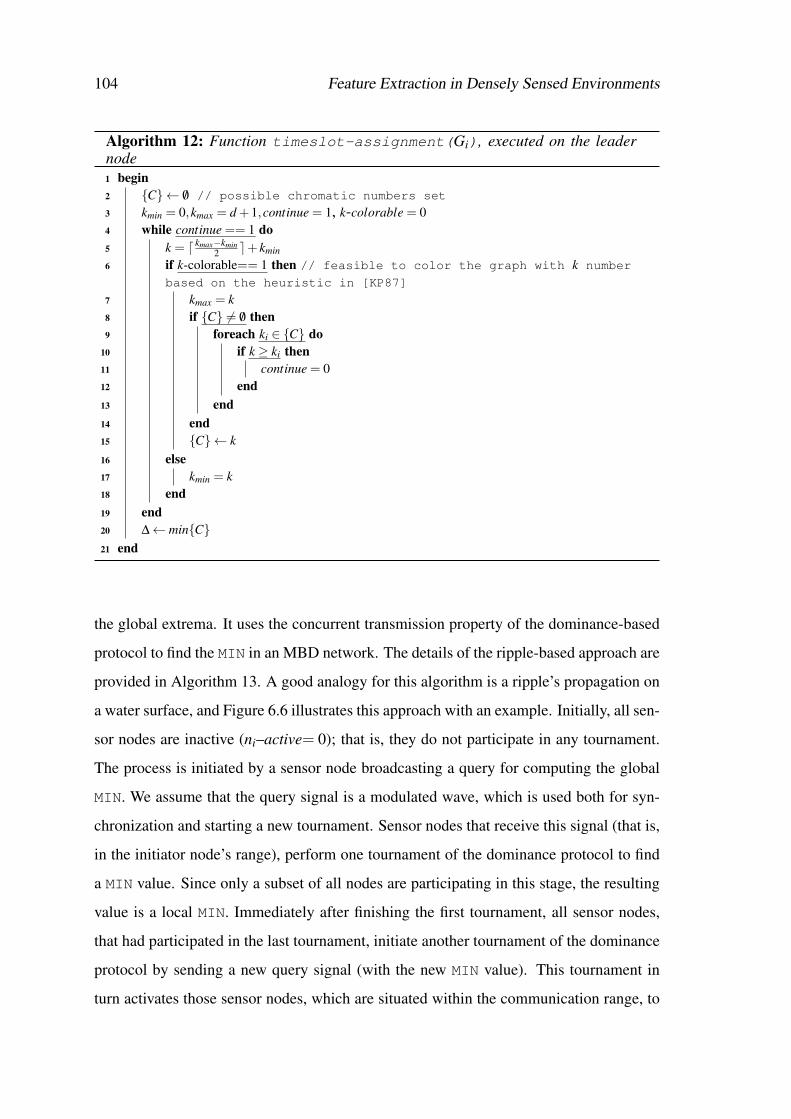
104 Feature Extraction in Densely Sensed Environments
Algorithm 12: Function timeslot-assignment(Gi), executed on the leadernode
1 begin
2 {C}← /0 // possible chromatic numbers set
3 kmin = 0,kmax = d +1,continue = 1, k-colorable = 04 while continue == 1 do
5 k = ⌈ kmax−kmin2 ⌉+ kmin
6 if k-colorable== 1 then // feasible to color the graph with k number
based on the heuristic in [KP87]
7 kmax = k
8 if {C} 6= /0 then
9 foreach ki ∈ {C} do
10 if k ≥ ki then
11 continue = 012 end
13 end
14 end
15 {C}← k
16 else
17 kmin = k
18 end
19 end
20 ∆← min{C}21 end
the global extrema. It uses the concurrent transmission property of the dominance-based
protocol to find the MIN in an MBD network. The details of the ripple-based approach are
provided in Algorithm 13. A good analogy for this algorithm is a ripple’s propagation on
a water surface, and Figure 6.6 illustrates this approach with an example. Initially, all sen-
sor nodes are inactive (ni–active= 0); that is, they do not participate in any tournament.
The process is initiated by a sensor node broadcasting a query for computing the global
MIN. We assume that the query signal is a modulated wave, which is used both for syn-
chronization and starting a new tournament. Sensor nodes that receive this signal (that is,
in the initiator node’s range), perform one tournament of the dominance protocol to find
a MIN value. Since only a subset of all nodes are participating in this stage, the resulting
value is a local MIN. Immediately after finishing the first tournament, all sensor nodes,
that had participated in the last tournament, initiate another tournament of the dominance
protocol by sending a new query signal (with the new MIN value). This tournament in
turn activates those sensor nodes, which are situated within the communication range, to

6.5 Computing Global Extrema in MBD Networks 105
Algorithm 13: Ripple-based approach, executed on each sensor node ni
1 begin
2 ni–active= 0, i = 03 while i≤ 2×⌈D/Rco⌉ do
4 i++
5 if ni–active== 1 then broadcast the query signal6 else if ni receives a query signal then
7 ni–active= 18 end
9 execute one dominance round
10 end
11 end
change their status from idle to tournament state. This procedure continues until all nodes
get activated.
To compute the global MIN in an MBD network, the tournament needs to be run in
worst case N = 2×⌈ DRco⌉ times where, D is the network diameter in number of hops and
Rco is the communication range of sensor nodes. Note that this is an upper-bound on the
number of tournaments that needs to be performed till all nodes in the network become
aware of MIN. Figure 6.7 reveals the rationale behind this process with an example. This
bounding event occurs when the sensor node with the lowest value and the initiator node
are located at opposite ends of the network (that is, initiator is D hops away from the sen-
sor with the lowest value). Hence, it takes twice the length of DRco
to assure that the MIN
value is propagated to all sensor nodes. The N times execution of the tournament is cor-
responding to one application of M function, or simply, one round in the MBD network.
At the end of each round, the winner node broadcasts a packet which includes its loca-
tion information and its identifier. This message is then flooded throughout the network,
using the ripple-based approach, such that all nodes have the same knowledge about the
properties of the winning node. Note that, in SBD, this information is broadcasted once
by the winner.
Figure 6.8 shows an example of computing MIN in an MBD network, where the place
of each node is represented by its measured value. In this example, we assume that the
node located at the center of the network initiates the query for computing MIN (see
Figure 6.8-a). Sensor nodes in the communication range of the initiator execute one

106 Feature Extraction in Densely Sensed Environments
Global MIN
Initiative
Figure 6.7: An example of the worst case scenario to determine the required number oftournament (N ). Assuming D = 12
√2 and Rco = 2
√2, the number of tournaments will
be N = 2× ⌈ DRco⌉ = 12, i.e. two times the number of circles depicted in this figure.
It takes six tournaments to activate the node with MIN and another six tournaments toreceive back the global MIN by the initiative sensor node.
tournament. Since nodes that are located in the border of the communication range of the
initiator are not reachable by each other, border sensor nodes find different MIN values
according to their location.
Figure 6.8-b shows the result of finding MIN after execution of the first tournament.
The two local MIN values (1 and 2) are propagated in the first tournament. In the next
iteration, all activated nodes perform the tournament and update their MIN values (see
Figure 6.8-c). Finally, after five tournaments, the global MIN is known throughout the
network.
However, the multi-hop protocol described above can suffer from the hidden terminal
problem. As dominance-based protocols allow nodes to listen to MIN value even from
simultaneous receptions, hidden terminals in this case can cause a device in the middle,
to learn a spurious MIN value.
To elaborate, consider three sensor nodes N1, N2 and N3 (with measured values 1, 2
and 3, respectively) as depicted in Figure 6.9. According to dominance-based protocols,
during the tournament a sensor node transmits its measured value bit-by-bit. Upon know-
ing the existence of other nodes with a smaller measured value, it stops sending the rest
of the bits. Now consider the scenario given in Figure 6.9-b. Node N3 loses the tourna-
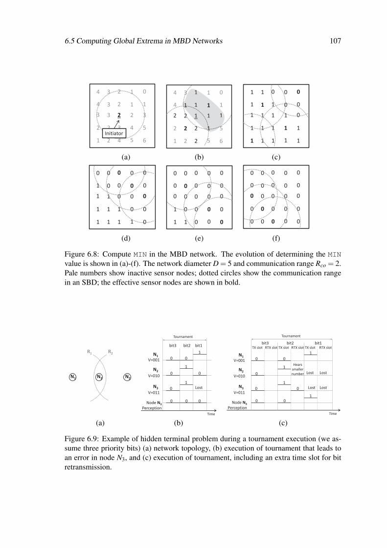
6.5 Computing Global Extrema in MBD Networks 107
4 3 2 1 0
1
3
5
6
1
1
2 2
2
2 2
4
4
3
3 3
4 2
5
3
Initiator
4 3 1 1 0
1
1
5
6
1
1
2 2
2
1 1
1
2
1
2 2
4 1
5
2
1
1
55
1
1 1
11
1 1
1 1 0 0 0
0
0
1
1
0
1
1 1
1
1 1
1
1
1
1 1
1 1
1
1
(a) (b) (c)
0 0 0 0 0
0
0
0
0
0
1
1 1
1
0 0
0
1
0
1 1
1 0
1
1
0 0 0 0 0
0
0
0
0
0
1
1 0
1
0 0
0
0
0
0 0
0 0
0
0
0 0 0 0 0
0
0
0
0
0
0
0 0
0
0 0
0
0
0
0 0
0 0
0
0
(d) (e) (f)
Figure 6.8: Compute MIN in the MBD network. The evolution of determining the MINvalue is shown in (a)-(f). The network diameter D = 5 and communication range Rco = 2.Pale numbers show inactive sensor nodes; dotted circles show the communication rangein an SBD; the effective sensor nodes are shown in bold.
N1
N3
N2
R2
R1 N
1
N3
N2
V=011
V=010
V=001
bit3 bit2 bit1
0
0
0
0
1
0
Node N3
Perception
0
1
0
1
Lost
0
Time
Tournament
N1
N3
N2
V=011
V=010
V=001
bit3 bit2 bit1
0
0
0
0
1
0
Node N3
Perception
0
1
1
Lost
Time
Tournament
TX slot RTX slot TX slot RTX slot
0
Hears
smaller
number Lost Lost
TX slot RTX slot
Lost
1
(a) (b) (c)
Figure 6.9: Example of hidden terminal problem during a tournament execution (we as-sume three priority bits) (a) network topology, (b) execution of tournament that leads toan error in node N3, and (c) execution of tournament, including an extra time slot for bitretransmission.

108 Feature Extraction in Densely Sensed Environments
ment after receiving the smallest value from node N1. Since node N1 and N2 are not able
to communicate directly, node N2 proceeds sending its last bit, which is 0, and node N3
mistakenly perceives MIN in the network as being 0.
To avoid this problem, we consider two slots for each bit transmission as proposed
in [PATR07]. The first slot is dedicated to the bit transmission itself and the second slot is
dedicated to the retransmission of the bit detected during the first slot. If the current bit of
a sensor node is dominant, there is no need to retransmit this bit for the second time, but
if the bit is recessive and the sensor node detects a dominant bit during the transmission
slot, it retransmits a dominant bit in the following retransmission slot (see Figure 6.9-c).
This bit-level redundancy solves the problem and leads to the correct perception of MIN
in the network. Obviously, it will increase the tournament duration.
6.6 Evaluation
We evaluated our proposed approaches in different simulated scenarios by considering
the following three metrics:
Number of Rounds. A sensor node gets channel-access permit to broadcast a message
in one round of execution of the M function if its value is the global minimum. Hence,
the number of rounds corresponds to the number of message broadcast or flooding.
Accuracy. It represents the fraction of sensor nodes that declare themselves to be lo-
cated in the active region(s) Ndet to the number of sensor nodes that truly lie in the active
region(s) Ntrue:
Accuracy =Ndet
Ntrue×100(%). (6.7)
In cases where the detected area is larger than the actual active region, (Ndet > Ntrue),
accuracy is more than 100%, which signifies the overestimation of the active region.
Execution Time. It is the time needed to extract the various features according to the
proposed augmenting functions and is computed as follows:

6.6 Evaluation 109
Execution Time = Number of Rounds×TM (6.8)
where, TM is the execution time of the M function. In SBD networks, TM is equal to one
tournament duration. However, in MBD networks, TM depends on the approach used for
computing the global extrema (as discussed in Section 6.5).
We first show the process of computing TM in MBD networks, and then evaluate the
feature extraction techniques for various exemplifying scenarios.
6.6.1 Computing the Execution Time of M Function, TM
As stated earlier, the application of M function results in identifying the global MIN over
values of sensor nodes in a shared medium.
We consider a network of size 100×100 sensor nodes in a shared medium. We change
the communication range of sensor nodes Rco to study the performance of the new ripple-
based and the classical cluster-based approaches in scenarios where the communication
range of the sensor nodes would divide the network into multiple broadcast domains. For
the cluster-based approach, where clusters are built based on a virtual range, we set the
range of virtual communication r, to be always half of the actual communication range
(Rco) of the sensor nodes.
To have a precise computation of a tournament round, we consider the timeouts as
given in Section 4.4.1, Table 4.4. As illustrated in Figure 6.9 to solve the hidden termi-
nal problem in the ripple-based approach, it is needed to send each bit twice during the
tournament. Considering 110µs as the length of one bit exchange, the tournament takes
110×nprio+ηµs for the cluster-based approach and 2×110×nprio+ηµs for the ripple-
based approach where, nprio is the number of priority bits and η is the time overhead
imposed by the MAC protocol during the tournament. This extra time overhead is mainly
due to synchronization and hardware shortcomings. For nprio = 15, the value of extra
time overhead is η = 3099µs. Accordingly, the tournament takes 4749µs and 6399µs for
the cluster-based and the ripple-based approaches, respectively.

110 Feature Extraction in Densely Sensed Environments
Table 6.2: Computation time of the MIN value in the cluster-based and the ripple-basedapproaches
CommunicationCluster-based Ripple-based
(Rco,r) (Rco)range Tnmta Time(µs) Tnmta Time(µs)
Rco = 14, r = 7 12 159388 8 96248Rco = 20, r = 10 10 137602 5 64763Rco = 28, r = 14 10 141698 4 50172Rco = 34, r = 17 11 150543 3 39677Rco = 40, r = 20 10 137602 3 35581
aNumber of referenced tournaments.
Table 6.2 shows the number of referenced tournaments along with the time needed to
find the global extremum in an MBD network. In this computation we took into account
the time needed to aggregate data in the case of the cluster-based approach, as well as
the time required for flooding the local information of the winner in the ripple-based ap-
proach. However, in both cases we assume the best case scenario. For data aggregation
through the black-node tree, we first compute the maximum degree d of the cluster inter-
fering graph (see Figure 6.5-a). To prevent any collision, it is considered that we need to
have at least d time-slots to collect data in the leader node. The duration of the time-slot is
considered to be the time needed to transmit a 128 byte-size packet. Assuming the IEEE
802.15.4-compliant MICAz’s radio [CRO04] with data rate of 250 Kb/s, the time-slot
duration (Ts) is then 4096µs.
For the ripple-based approach, we compute the flooding time according to the theo-
retical lower latency bound given in [FZTS11]. In that work, the authors simplify that
given that nodes transmit concurrently, the theoretical lower latency bound in a network
with size h hops is h.(Ts+Td). The number of hops is computed as h = ⌈ DRco⌉, where D is
the network diameter and Rco is the communication range of sensor nodes. Td is the radio
processing delay, which is in the order of a few microseconds and is determined by the
radio; for simplicity, we ignore Td in our computation.
As expected, increasing the communication range results in a faster computation of
MIN with the ripple-based approach. Also, this method needs a smaller number of tourna-
ments as compared to the cluster-based approach. However, in the cluster-based approach,

6.6 Evaluation 111
we do not observe the same continuous descending trend in the number of referenced tour-
naments. The reason is that the placement of the clusters plays an important role in the
construction of the black-node tree and the cluster interfering graph that affects the d
value.
It should be mentioned that the given time for both approaches is slightly optimistic.
In the cluster-based approach, we do not consider the extra overhead imposed by the
setup phase for cluster formation and similarly in the ripple-based approach we have used
the lower bound of the flooding delay as in [FZTS11]. Note that in the cluster-based
approach, not all sensor nodes become aware of MIN, while, in the ripple-based approach,
which is a fully distributed algorithm, all nodes would know MIN.
6.6.2 Identifying the Active Regions
We consider the same network settings as described in the previous subsection, with the
size of 100×100 sensor nodes. First, we show the performance of distance augmenting
function to identify circular active regions. For evaluating our approach, we generate
various scenarios with several active regions. The active regions may or may not overlap
resulting in complex fields. The details of the scenarios are provided in Figure 6.10.
In each round of execution, after finding the global maximum, all the sensor nodes
compute local values of φβ according to Equation 6.1. Figure 6.11 illustrates the number
of circular active regions with different termination rules for scenario sc1. Increasing the
threshold level helps the algorithm to converge faster in smaller number of rounds, but at
the cost of reduced accuracy.
Figure 6.12 shows the number of rounds and the corresponding obtained accuracy for
different threshold values. We believe that the property of the field plays an important
role on the number of required rounds and on the accuracy of the detection. In some
scenarios, increasing the termination threshold reduces the number of rounds as well as
the overestimated area. This happens for scenarios sc1, sc3 and sc6, where the active
regions can overlap. However, for scenarios sc2, sc4 and sc5, where either few active
regions exist or active regions are far apart, the number of rounds and the accuracy remains
almost the same for all termination conditions. The existence of isolated peaks in the field

112 Feature Extraction in Densely Sensed Environments
x−axis
y−
ax
is
0 20 40 60 80 1000
20
40
60
80
100
x−axis
y−
ax
is
0 20 40 60 80 1000
20
40
60
80
100
(sc1) (sc2)
x−axis
y−
ax
is
0 20 40 60 80 1000
20
40
60
80
100
x−axis
y−
ax
is
0 20 40 60 80 1000
20
40
60
80
100
(sc3) (sc4)
x−axis
y−
ax
is
0 20 40 60 80 1000
20
40
60
80
100
x−axis
y−
ax
is
0 20 40 60 80 1000
20
40
60
80
100
(sc5) (sc6)
Figure 6.10: Six scenarios with different active regions; each sensor node sets the valueof β = 10 to compute its priority —see Equation (6.1-6.3). Each circle represents onefiltering zone that is computed by two readings from the sensor network and excludessensor nodes located inside the circle from participation in the future iteration(s) of thealgorithm. πs is set to 10% of the global maximum value.

6.6 Evaluation 113
x−axis
y−
ax
is
0 20 40 60 80 1000
20
40
60
80
100
x−axis
y−
axis
0 20 40 60 80 1000
20
40
60
80
100
(a) (b)
Figure 6.11: The effect of termination threshold, πs on the detection of active regions.The algorithm terminates when a new detected peak is (a) 20% and (b) 30% of the globalmaximum value.
sc1 sc2 sc3 sc4 sc5 sc60
10
20
30
40
50
Scenarios
Nu
mb
er
of
rou
nd
s [
bar
ch
art
]
30% 20% 10%
0
50
100
150
200
250
Accu
racy (
%)
[lin
e c
hart
]
10% 20% 30%
30%10%
Figure 6.12: The number of rounds and the accuracy of active region estimation under thedifferent scenarios for various πs = {10%,20%,30%} of the global maximum.
sc2 sc4 sc50
50
100
150
200
Scenarios
Ac
cu
rac
y (
%)
β = 13
β = 15
β = 20
β = 40
β = 50
β = 60
Figure 6.13: The effect of β on the accuracy.

114 Feature Extraction in Densely Sensed Environments
sc1 sc2 sc3 sc4 sc5 sc60
1000
2000
3000
4000
5000
Execu
tio
n T
ime (
ms)
Scenarios
C(14,7) C(40,20) R(14) R(40)
Figure 6.14: Execution time of Aβ (β = 10, πs = 20%) in an MBD network with differ-ent communication ranges for the cluster-based approach: {C(14,7), C(40,20)} and theripple-based approach: {R(14), R(40)}.
results in identifying all active regions by a fixed number of circular sections. The high
value of overestimation in sc4 and sc5 is due to the steepness of the peak in the field. This
steepness causes an overestimation in the filtering radius which in turn leads to a much
larger (squared) overestimation of the circle’s area.
We found that the choice of the exponential coefficient β in our given heuristic (Equa-
tion 6.3) affects the overestimation of active regions. In fact, the coefficient β impacts the
relative weight of distance from the peak with respect to the value of the field at a given
point. Choosing an optimal value of β is not possible without the prior knowledge of the
field, but the order of β can be chosen based on the size of the field such that a proper
trade-off between the sensor value at a given sensor node and its distance from the peak
is maintained. Particularly, β should be chosen such that the impact of distance can be
pronounced as compared to the distance normalization (dmax in Equation 6.3). For an area
of 100×100, we found that suitable values of β are in the order of 10. Specific results on
the accuracy for the scenarios sc2, sc4 and sc5 are shown in Figure 6.13. The main goal
of this experiment is to investigate the level of overestimation given by Aβ . It is observed
that for scenarios with isolated peaks, higher values of β improve the coverage estimation
accuracy (β = 40 for scenario sc4 and β = 60 for scenario sc5). But for scenarios where
the spread of peaks overlap, the effect of changing β is less pronounced, as in the case of
scenario sc2.
Figure 6.14 shows the time it takes to detect the location of active regions by Aβ .

6.6 Evaluation 115
We examined the performance of the cluster-based and the ripple-based approaches for
different communication ranges Rco = {14,40}, which are the extreme ranges (shortest
and longest) in Table 6.2 . Interestingly, the execution time of Aβ under the ripple-based
approach is at least 58% faster than that for the cluster-based approach. Increasing the
communication range from Rco = 14 to Rco = 40 leads the algorithm to be 63% faster
under the ripple-based approach while it improves the cluster-based approach only by
34%.
6.6.3 Convex-hull Around Active Regions
For evaluating the convex-hull approach described in Section 6.4.2, we convert the field
to a binary field by thresholding, such that a sensor node’s value is 1 if the sensed value
is greater than 10% of the maximum value, and 0 otherwise. The details of the scenarios
are provided in Figure 6.15. We set the marginal extension angle to ε = 1◦ and γ = 1.
We compared our technique with a TDMA approach, where a fixed number of randomly
chosen sensor nodes send their measurements. For the random approach, the number of
readings was set to 150.
Figure 6.16 shows the accuracy of our second technique in terms of average per-
centage of coverage area by running the simulation over 100 iterations. As shown, our
technique covers more than 97% of the area in all the scenarios through transmitting 26 to
33 broadcast messages compared to 36% to 72% coverage by 150 randomly chosen pack-
ets. Hence, we acquire a more accurate boundary estimation with 77% less broadcast
messages.
Increasing the marginal extension angle, ε , still provides a satisfactory coverage area
estimation, while reducing the number of messages. We tested the performance of our
proposed algorithm with different marginal extension angles in all the mentioned scenar-
ios. As shown in Figure 6.17, by increasing ε , the number of rounds decreases, since by
enlarging the angle, more search space is filtered out and consequently less packets are
needed to be broadcast.
However, increasing ε might diminish the performance of the algorithm in terms of
estimated coverage area. Figure 6.18 shows the performance degradation by increasing

116 Feature Extraction in Densely Sensed Environments
x−axis
y−
ax
is
0 20 40 60 80 1000
20
40
60
80
100
x−axis
y−
axis
0 20 40 60 80 1000
20
40
60
80
100
(sc1) (sc2)
x−axis
y−
axis
0 20 40 60 80 1000
20
40
60
80
100
x−axis
y−
ax
is
0 20 40 60 80 1000
20
40
60
80
100
(sc3) (sc4)
x−axis
y−
axis
0 20 40 60 80 1000
20
40
60
80
100
x−axis
y−
axis
0 20 40 60 80 1000
20
40
60
80
100
(sc5) (sc6)
Figure 6.15: Six scenarios with different active regions; solid lines show the boundarycomputed by our algorithm with ε = 1◦ and 40 iterations of the algorithm, and dash linesshow the boundary computed by the random algorithm with 150 random readings.
the ε up to 90◦. Under the latter setting, the proposed algorithm is able to cover around
70% of the active region. In addition to the shown value of ε in the graph, we also ran
the simulation for ε = {5◦,10◦} and took the standard deviation of the average coverage
area for ε = (1◦ : ε). Since the results for ε = {5◦,10◦} were very close to the case where
ε = 1◦, the coverage area computed by these values is not shown in the figure. As can
be seen in Figure 6.18, ε = 15◦ has the smallest standard deviation (smaller than 0.65),
which suggests that the coverage area computed by ε = 15◦ leads to the same coverage
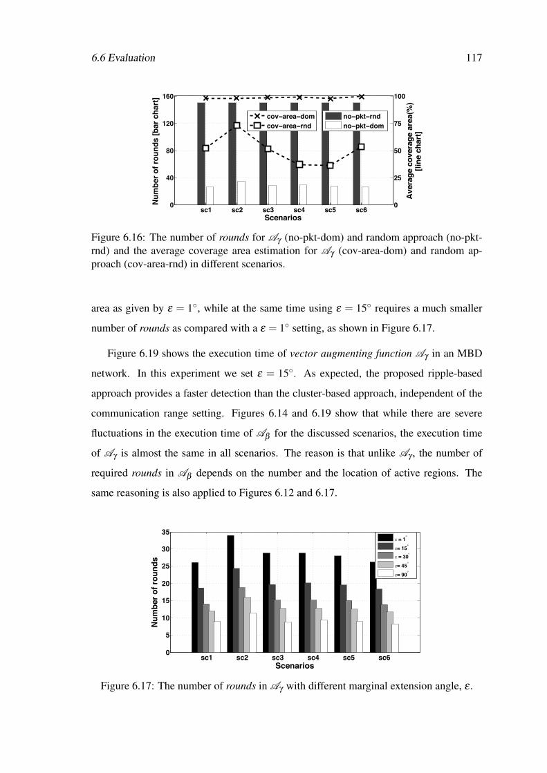
6.6 Evaluation 117
sc1 sc2 sc3 sc4 sc5 sc60
40
80
120
160
Scenarios
Nu
mb
er
of
rou
nd
s [
bar
ch
art
]
no−pkt−rnd
no−pkt−dom
0
25
50
75
100
Avera
ge c
overa
ge a
rea(%
)[l
ine c
hart
]
cov−area−dom
cov−area−rnd
Figure 6.16: The number of rounds for Aγ (no-pkt-dom) and random approach (no-pkt-rnd) and the average coverage area estimation for Aγ (cov-area-dom) and random ap-proach (cov-area-rnd) in different scenarios.
area as given by ε = 1◦, while at the same time using ε = 15◦ requires a much smaller
number of rounds as compared with a ε = 1◦ setting, as shown in Figure 6.17.
Figure 6.19 shows the execution time of vector augmenting function Aγ in an MBD
network. In this experiment we set ε = 15◦. As expected, the proposed ripple-based
approach provides a faster detection than the cluster-based approach, independent of the
communication range setting. Figures 6.14 and 6.19 show that while there are severe
fluctuations in the execution time of Aβ for the discussed scenarios, the execution time
of Aγ is almost the same in all scenarios. The reason is that unlike Aγ , the number of
required rounds in Aβ depends on the number and the location of active regions. The
same reasoning is also applied to Figures 6.12 and 6.17.
sc1 sc2 sc3 sc4 sc5 sc60
5
10
15
20
25
30
35
Scenarios
Nu
mb
er o
f ro
un
ds
ε = 1°
ε= 15°
ε = 30°
ε= 45°
ε= 90°
Figure 6.17: The number of rounds in Aγ with different marginal extension angle, ε .

118 Feature Extraction in Densely Sensed Environments
sc1 sc2 sc3 sc4 sc5 sc660
70
80
90
100
Scenarios
Avera
ge c
overa
ge a
rea(%
)[b
ar
ch
art
]
0
3
6
9
12
Sta
nd
ard
Devia
tio
n [
lin
e c
hart
]
ε=1°
ε=15°
ε=30°
ε=45°
ε=90°
ε=15°
ε=30°
ε=45°
ε=90°
Figure 6.18: The average of estimated coverage area with different marginal extensionangle, ε and its standard deviation.
sc1 sc2 sc3 sc4 sc5 sc60
1000
2000
3000
4000
5000
6000
Execu
tio
n T
ime (
ms)
Scenarios
C(14,7) C(40,20) R(14) R(40)
Figure 6.19: Execution time of Aγ (γ = 1,ε = 15◦) in an MBD network with differ-ent communication ranges for the cluster-based approach: {C(14,7), C(40,20)} and theripple-based approach: {R(14), R(40)}.
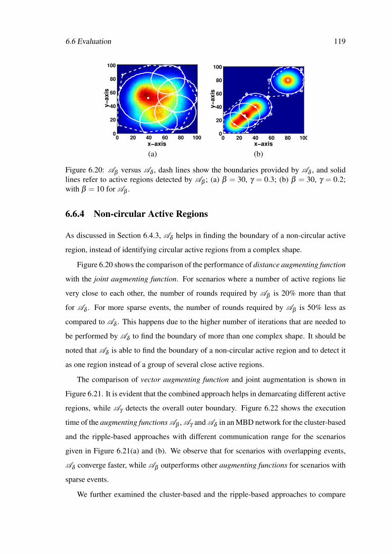
6.6 Evaluation 119
x−axis
y−
ax
is
0 20 40 60 80 1000
20
40
60
80
100
x−axis
y−
ax
is
0 20 40 60 80 1000
20
40
60
80
100
(a) (b)
Figure 6.20: Aβ versus Aδ , dash lines show the boundaries provided by Aδ , and solidlines refer to active regions detected by Aβ ; (a) β = 30, γ = 0.3; (b) β = 30, γ = 0.2;with β = 10 for Aβ .
6.6.4 Non-circular Active Regions
As discussed in Section 6.4.3, Aδ helps in finding the boundary of a non-circular active
region, instead of identifying circular active regions from a complex shape.
Figure 6.20 shows the comparison of the performance of distance augmenting function
with the joint augmenting function. For scenarios where a number of active regions lie
very close to each other, the number of rounds required by Aβ is 20% more than that
for Aδ . For more sparse events, the number of rounds required by Aβ is 50% less as
compared to Aδ . This happens due to the higher number of iterations that are needed to
be performed by Aδ to find the boundary of more than one complex shape. It should be
noted that Aδ is able to find the boundary of a non-circular active region and to detect it
as one region instead of a group of several close active regions.
The comparison of vector augmenting function and joint augmentation is shown in
Figure 6.21. It is evident that the combined approach helps in demarcating different active
regions, while Aγ detects the overall outer boundary. Figure 6.22 shows the execution
time of the augmenting functions Aβ , Aγ and Aδ in an MBD network for the cluster-based
and the ripple-based approaches with different communication range for the scenarios
given in Figure 6.21(a) and (b). We observe that for scenarios with overlapping events,
Aδ converge faster, while Aβ outperforms other augmenting functions for scenarios with
sparse events.
We further examined the cluster-based and the ripple-based approaches to compare

120 Feature Extraction in Densely Sensed Environments
x−axis
y−
ax
is
0 20 40 60 80 1000
20
40
60
80
100
x−axis
y−
ax
is
0 20 40 60 80 1000
20
40
60
80
100
(a) (b)
Figure 6.21: Aγ versus Aδ , dash lines show the boundaries provided by Aδ and solidlines refer to that given by Aγ (a) β = 30, γ = 0.3; (b) β = 30, γ = 0.2; with ε = 15◦ forAγ .
0
500
1000
1500
2000
2500
Execu
tio
n T
ime (
ms)
Techniques
C(14,7) C(40,20) R(14) R(40)
Aγ
Aδ
Aβ
0
1000
2000
3000
4000
Ex
ec
uti
on
Tim
e (
ms
)
Techniques
C(14,7) C(40,20) R(14) R(40)
Aδ
Aβ
Aγ
(a) (b)
Figure 6.22: Execution time of different augmenting functions in an MBD networkwith different communication ranges for cluster-based approach {C(14,7), C(40,20)} andripple-based approach {R(14), R(40)}: (a) considering scenarios depicted in (Figure 6.21-a) and (b) considering scenarios depicted in (Figure 6.21-b).
(14,7) (20,10) (28,14) (34,17) (40,20)0
500
1000
1500
2000
2500
3000
3500
4000
4500
5000
5500
6000
Communication range (R, r)
Execu
tio
n T
ime (
ms)
Aβ, Cluster−based
Aγ, Cluster−based
Aδ, Cluster−based
Aβ, Ripple−based
Aγ, Ripple−based
Aδ, Ripple−based
Figure 6.23: The computation time of various feature extraction techniques (Aβ , Aγ andAδ ) for scenario sc2 with πs = 20%, ε = 15◦, γ = 1, θ = π/4.

6.6 Evaluation 121
0
5
10
15
20
25
30
TechniquesN
um
be
r o
f ro
un
ds
100x100
300x300
500x500
Aγ
Aβ
Aδ
Figure 6.24: The impact of density on the performance of each technique for scenariosc2.
the time needed to extract different features according to the augmenting functions given
in Section 6.4 for a single scenario. Figure 6.23 shows the elapsed time for different
augmenting functions (Aβ , Aγ , Aδ ) for the sample scenario sc2 over a 100×100 network.
We chose this scenario because, according to the results in Section 6.6, this scenario
includes the most complex field. It is evident that for all communication range settings,
and for all augmenting functions, the proposed ripple-based approach outperforms the
classical cluster-based approach.
6.6.5 The Impact of Network Density
Finally, we compare our techniques under various network densities. As our techniques
only depend on collecting the global extrema of various augmenting functions, the re-
sults indicate that increasing the network density has almost no impact on the number of
rounds. Figure 6.24 shows the number of rounds required in each technique with respect
to the network size. The slight variation in the number of rounds is due to the effect of
termination condition in Aβ and the randomness in the choice of θ in Aγ .
6.6.6 Alternative Flooding Approaches
Many emerging cyber physical systems need mechanisms to share and process data among
all devices in the network. The ripple-based approach, proposed in this work, is one such
mechanisms, in the sense that it computes an aggregate quantity over all the devices.
Chaos [LFZ13] and Low-power Wireless Bus (LWB) [FZMT12] are two other examples
122 Feature Extraction in Densely Sensed Environments
of such mechanisms that build their data collection or dissemination capabilities based on
the Glossy protocol [FZTS11].
Since we aim at obtaining an efficient and scalable algorithm with low time-complexity,
we compare the performance of different flooding approaches based on execution time
and scalability. Chaos outperforms LWB in terms of completion time [LFZ13]. In fact
Chaos is able to collect small amounts of data, such as a 1-byte payload, from a 100-node
network within less than 100 ms. We believe that there are two main advantages of our
proposed ripple-based approach over Chaos. Firstly it provides a faster execution time;
considering the tournament duration 6399 µs (see Section 6.6.1), in the ripple-based ap-
proach, all nodes will know MIN in at most 52 ms within a seven-hop network deployment.
Secondly, it offers better scalability; in fact while in Chaos the number of nodes is limited
to 856 in a SBD (unless some data compression mechanism is applied), our ripple-based
approach does not limit the number of involved devices.
6.7 Concluding Remarks
Low-power wireless sensor networks enable many emerging applications that need thou-
sands of sensor nodes for control and monitoring. In this chapter, we presented a set of
techniques that identify various features in the distribution of sensed physical quantities
over a dense deployment of sensor nodes. With such simple yet effective modifications,
we can obtain the location and shape of active regions with a number of messages propor-
tional to the properties of the field. Our feature extraction techniques are efficient in the
sense that they collect data from just the sensors that have more effective information for
revealing the status of the monitored area.
We proposed a fully distributed approach to make our feature extraction scale with
large dense networks, where sensor nodes lie in a multiple broadcast area.

Chapter 7
Conclusions, Perspective and Future
Directions
This chapter reviews the research objectives of the Thesis and summaries its major re-
sults, highlighting how the research contributions fulfilled the original research objectives.
Some guidelines for future research work in the area are also provided.
7.1 Summary of the Work
In this work we aimed at designing large-scale dense networked sensor systems where the
sensing is performed at a very fine granularity, both in space and time. Previous research
work [APE+08, ETPA11, PGAT09] has proposed algorithms for obtaining an interpola-
tion of sensor readings from different sensor nodes, and these algorithms are based on
dominance protocols, presenting therefore excellent scalability properties for densely in-
strumented CPS. We believe however that it was possible to improve the performance
of those algorithms not only by taking advantage of knowledge of often-occurring spa-
tial correlation of sensor readings but also by embedding the dynamics of the physical
phenomenon in the algorithms. We further proposed efficient novel mechanism able to
extract meaningful features from the high spatial resolution of sensor readings utilizing
the same building block as used for obtaining the interpolation: MIN.
123

124 Conclusions, Perspective and Future Directions
7.1.1 Review of Research Objectives
To address the problem of reliable and timely data transmission and data aggregation in
dense sensing networks, we defined the following three theoretical objectives:
1. Devising an error recovery scheme for WiDOM protocol in a noisy wireless chan-
nel.
2. Devising a mechanism that captures the dynamics of the physical quantities and self
adapts according to the physical changes.
3. Devising a set of algorithms to identify various features in a distribution of a physical
quantity.
7.1.2 Main Research Contributions
Next we briefly summarize the main research contributions.
Improving the reliability of the wireless communication infrastructure. Sensor
nodes must communicate using a shared broadcast medium (such as a shared bus or a
wireless channel), as it would be unfeasible (due to the number of nodes) to deploy ded-
icated communication channels for each sensor/actuator node. The WiDOM protocol is
known as a MAC protocol suitable to be exploited to allow computation of aggregate
quantities in wireless. In order to reduce the large overhead of the WiDOM protocol,
the slotted WiDOM was proposed. However, none of these designs were considered to
tolerate errors that may occur in data transmissions. One of the main contributions of
this research work is the introduction of an error recovery scheme able to significantly
improve the reliability of the WiDOM protocol and as such to increase the utility of the
approach for computing complex aggregate quantities. We develop this scheme over slot-
ted WiDOM since it offers lower overhead as compared to the original WiDOM design.
Developing scalable and efficient aggregate quantities that consider the physical
dynamics. Previous works tackling densely deployed networked sensor systems have
proposed algorithms that allow computing an approximate interpolation of sensor read-
ings by exploiting dominance-based protocols. The second main contribution in this The-
sis is a novel approach for computing approximate interpolations, where the algorithm is

7.2 Future Directions 125
self-adaptable to incorporate the physical dynamics and the trade-offs between accuracy
and timeliness.
Extracting various features from the distribution of the physical quantity being
monitored. Many CPS applications need to detect regions with specific level of activ-
ities immediately after the occurrence of an event. While computing the interpolation
together with a centralized signal processing technique might be considered as an option,
we devised a set of fully distributed algorithms that provide meaningful information from
the distribution of the physical quantity without the need of having the interpolated im-
age. We showed that similarly to the case of interpolation algorithm, the time complexity
of the novel algorithms depends only on the property of the distribution of the physical
quantity.
Extending the feature extraction algorithm to multi-hop networked infrastruc-
tures. To extend the devised algorithm to work in a multi-hop network, we devised
a distributed approach that takes advantage of dominance-based protocol. We further
examined the functionality of the proposed multi-hop approach against the traditional
cluster-based approach and revealed that our novel approach outperforms the traditional
approaches.
7.1.3 Validation of the Hypothesis
We have shown through extensive evaluations that it is possible to extract
certain features of a physical phenomenon in a dense sensing network with a
time complexity that is independent of the number of sensor nodes.
7.2 Future Directions
There are several opportunities that can be identified for further research:
– Devising distributed algorithms for extracting other features or computing dif-
ferent aggregate quantities over a distribution of a physical quantity (related
to Chapter 6). It is shown that the efficient computation of MIN through exploit-
ing dominance-based protocol can serve as the basic building block for extracting

126 Conclusions, Perspective and Future Directions
different features from a physical signal. Leveraging MIN computation would even-
tually be considered to further develop other aggregation algorithms.
– Implementing the feature extraction algorithms on a real dense sensor plat-
form using WiDOM protocol (related to Chapter 6). An experiment is required,
using a test bed, to implement a dense sensor network to observe a phenomena
and verify the results discussed in Chapter 6. Along this line, improvements to the
proposed feature extraction algorithm would be required, by developing a proper
synchronization algorithm for the MBD network, in order to increase its reliability.
Furthermore, the limitations imposed by communication medium may also have to
be considered. The current platform that exists for slotted WiDOM is a prototype
developed from components commercially available at the time [PGAT09]. The
development and research of better radios for the execution of slotted WiDOM and
hardware miniaturization are two topics that would enable practical implementation
of the proposed algorithm in a wireless domain.
– Development of an adaptive interpolation algorithm for accommodating non-
linear change patterns in an dynamic signal (related to Chapter 5). Proposed
interpolation algorithms consider fixed change rates of the signal [ETPA11]. In this
Thesis we solve the problem of dynamic change pattern for linear change model.
One interesting future work is to develop this scheme for non-linear change pat-
terns.
– Investigation of a more realistic noise pattern for wireless channel (related
to Chapter 4). To provide the RMA for hard real-time support in the slotted
WiDOM under noisy channel environment, the considered noise model was based
on the technique proposed in [BVT+10]. There is a need to have a better noise
model for real-time data traffic over wireless channel.
– Developement of a probabilistic end-to-end delay guarantee for the case that
no valid noise patterns exist (related to Chapter 4). In some scenarios, the RMA
deemed to be hardly applicable to wireless networks due to high error probability

7.2 Future Directions 127
associated with such networks. However, it must be mentioned that this is a techno-
logical problem. The reliability of wireless networks has evolved noticeably over
the last few years and hence, it is safe to assume that this evolution will continue.
Nonetheless, computing a probabilistic delay guarantee can also be considered as
a way to mitigate the constraint of hard real-time system and makes the protocol
applicable in the context of soft real-time QoS guarantee.

128 Conclusions, Perspective and Future Directions
Author’s List of Publications
The following publications have been derived from work directly related to this disserta-
tion:
Journals
• M. Vahabi, V. Gupta, M. Albano, R. Rangarajan and E. Tovar. Feature Extrac-
tion in Densely Sensed Environments: Extensions to Multiple Broadcast Domains.
International Journal of Distributed Sensor Networks (2015). (Accepted.)
• M. Vahabi, S. Tennina, E. Tovar and B. Andersson. Extended version of: Re-
sponse Time Analysis of Slotted WiDOM in Noisy Wireless Channels. (Under
submission.)
• M. Vahabi, E. Tovar. and M. Albano. Extended version of: A Self-Adaptive Ap-
proximate Interpolation Scheme for Dense Sensing. (Under submission.)
Conferences and Workshops
• M. Vahabi, E. Tovar. and M. Albano. A Self-Adaptive Approximate Interpolation
Scheme for Dense Sensing. In 8th IEEE International Symposium on Industrial
Embedded Systems (SIES 2013), pages 105–109, June 2013, Porto, Portugal. doi:
10.1109/SIES.2013.6601481.
• M. Vahabi, V. Gupta, M. Albano and E. Tovar. Feature Extraction in Densely
Sensed Environments. In 27th IEEE International Conference on Distributed Com-
puting in Sensor Systems (DCOSS 2014), pages 143-151, May 2014, Marina Del
Rey, U.S.A.. doi:10.1109/DCOSS.2014.29.
129

130 Conclusions, Perspective and Future Directions
• M. Vahabi, S. Tennina, E. Tovar and B. Andersson. Response Time Analysis of
Slotted WiDOM in Noisy Wireless Channels. Accepted to be presented in 20th
IEEE International Conference on Emerging Technologies and Factory Automation
(ETFA 2015), September 2015, Luxembourg.
Posters and Demos
• M. Vahabi, B. Andersson. New Schedulability Analysis for WiDom. Work-In-
Progress Session in conjunction with the 22nd EUROMICRO Conference on Real-
Time Systems (ECRTS 2010), 6, July, 2010. Brussels, Belgium.
• J. Loureiro, N. Pereira, E. Tovar, F. Pacheco, M. Vahabi. The SmartSkin Project:
Densely Instrumented Physical Infrastructures. In 1st Industrial Workshop on Real-
Time and Embedded Systems (CiWork 2013), Porto, Portugal.
• J. Loureiro, N. Pereira, E. Tovar, F. Pacheco, M. Vahabi. Reducing Aircraft Fuel
Consumption with WSAN-based Active Flow Control. In 1st Industrial Workshop
on Real-Time and Embedded Systems (CiWork 2013), Porto, Portugal.
Bibliography
[80206] IEEE Standard for local and metropolitan area networks - part
15.4: Low-Rate Wireless Personal Area Networks (LR-WPANs),
IEEE Std 802.15.4-2011 (Revision of IEEE Std 802.15.4-2006).
http://standards.ieee.org/getieee802/802.15.html, 2006.
[80212] IEEE Standard for Local and Metropolitan Area Networks–Part 15.4: Low-
Rate Wireless Personal Area Networks (LR-WPANs)–Amendment 1: MAC
Sublayer. https://standards.ieee.org/findstds/standard/802.15.4e-2012.html,
2012.
[AC01] Imad Aad and Claude Castelluccia. Differentiation Mechanisms for IEEE
802.11. In 20th Annual Joint Conference of the IEEE Computer and
Communications Societies (INFOCOM), volume 1, pages 209–218, 2001.
[AIM10] Luigi Atzori, Antonio Iera, and Giacomo Morabito. The Internet of Things:
A Survey. Computer networks, 54(15):2787–2805, 2010.
[APE+08] Björn Andersson, Nuno Pereira, Wilfried Elmenreich, Eduardo Tovar, Fil-
ipe Pacheco, and Nuno Cruz. A Scalable and Efficient Approach for Ob-
taining Measurements in CAN-Based Control Systems. IEEE Transactions
on Industrial Informatics (TII), 4(2):80–91, 2008.
[APT07] Björn Andersson, Nuno Pereira, and Eduardo Tovar. Exploiting a Priori-
tized MAC Protocol to Efficiently Compute Min and Max in Multihop Net-
works. In 5th Workshop on Intelligent Solutions in Embedded Systems,
pages 239–249. IEEE, 2007.
131

132 BIBLIOGRAPHY
[APT08] Björn Andersson, Nuno Pereira, and Eduardo Tovar. How a Cyber-Physical
System can Efficiently Obtain a Snapshot of Physical Information even in
the Presence of Sensor Faults. In International Workshop on Intelligent
Solutions in Embedded Systems, pages 1–10. IEEE, 2008.
[APT09] Björn Andersson, Nuno Pereira, and Eduardo Tovar. Estimating the Num-
ber of Nodes in Wireless Sensor Networks. 2009.
[AT06] Björn Andersson and Eduardo Tovar. Static-Priority Scheduling of Sporadic
Messages on a Wireless Channel. In Principles of Distributed Systems,
pages 322–333. Springer, 2006.
[ATS14] Besim Avci, Goce Trajcevski, and Peter Scheuermann. Managing Evolving
Shapes in Sensor Networks. In 26th International Conference on Scientific
and Statistical Database Management. ACM, 2014.
[BCV01] Michael Barry, Andrew T Campbell, and Andras Veres. Distributed Control
Algorithms for Service Differentiation in Wireless Packet Networks. In
20th Annual Joint Conference of the IEEE Computer and Communications
Societies (INFOCOM), volume 1, pages 582–590, 2001.
[BGHS06] Chiranjeeb Buragohain, Sorabh Gandhi, John Hershberger, and Sub-
hash Suri. Contour Approximation in Sensor Networks. In Distributed
Computing in Sensor Systems, pages 356–371. Springer, 2006.
[BLDB06] Reinder J Bril, Johan J Lukkien, Rob I Davis, and Alan Burns. Message Re-
sponse Time Analysis for Ideal Controller Area Network (CAN) Refuted.
5th Int. Work. on Real-Time Network (RTN), pages 5–10, 2006.
[Bos91] Bosch. CAN Specification version 2.0. Robert Bosch GmbH, Stuttgart,
pstfach 30 02 40, d-70442 edition, 1991.
[BVN+11] C.A. Boano, T. Voigt, C. Noda, K. Romer, and M. Zuniga. JamLab:
Augmenting Sensornet Testbeds with Realistic and Controlled Interference

BIBLIOGRAPHY 133
Generation. In 10th International Conference on Information Processing in
Sensor Networks (IPSN), pages 175 –186, 2011.
[BVT+10] C. Boano, T. Vigot, N. Tsiftes, L. Mottola, K. Romer, and M. Zuniga. Mak-
ing Sensornet MAC Protocols Robust Against Interference. In 7th European
Conference on Wireless Sensor Networks (EWSN), pages 272–288, 2010.
[CBBS03] Thomas W Carley, Moussa A Ba, Rajeev Barua, and David B Stewart.
Contention-Free Periodic Message Scheduler Medium Access Control in
Wireless Sensor/Actuator Networks. In 24th IEEE Real-Time Systems
Symposium (RTSS), pages 298–307, 2003.
[CG03] Krishna Kant Chintalapudi and Ramesh Govindan. Localized Edge Detec-
tion in Sensor Fields. Ad Hoc Networks, 1(2):273–291, 2003.
[CGJ+04] John Caffrey, Ramesh Govindan, Erik Johnson, Bhaskar Krishnamachari,
Sami Masri, Gaurav Sukhatme, Krishna Chintalapudi, Karthik Dantu,
Sumit Rangwala, Avinash Sridharan, et al. Networked Sensing for Struc-
tural Health Monitoring. In 4th International Workshop on Structural
Control, pages 57–66. Columbia University NY, 2004.
[CO05] Martin Connolly and Fergus O’Reilly. Sensor Networks and the Food In-
dustry. In 1st Workshop on Real-World Wireless Sensor (REAL WSN),
pages 20–21. Citeseer, 2005.
[COM09] EMBEDDED COMPUTING. Cyber-Physical Systems. 2009.
[CRO04] CROSSBOW. Datasheet: MICAz. Crossbow Technology, Inc, San Jose,
USA, 2004.
[CVV08] Gianluca Cena, Adriano Valenzano, and Stefano Vitturi. Hybrid
Wired/Wireless Networks for Real-Time Communications. IEEE Industrial
Electronics Magazine, 2(1):8–20, 2008.

134 BIBLIOGRAPHY
[CWKS97] Brian P Crow, Indra Widjaja, Jeong Geun Kim, and Prescott T Sakai. IEEE
802.11 Wireless Local Area Networks. IEEE Communications Magazine,
35(9):116–126, 1997.
[CZSB02] Marco Caccamo, Lynn Y Zhang, Lui Sha, and Giorgio Buttazzo. An
Implicit Prioritized Access Protocol for Wireless Sensor Networks. In
23rd Conference on Real-Time Systems Symposium (RTSS), pages 39–48.
IEEE, 2002.
[DBBL07] R. Davis, A. Burns, R. Bril, and J. Lukkien. Controller Area Net-
work (CAN) Schedulability Analysis: Refuted, Revisited and Revised.
Real-Time Systems, 35:239–272, 2007.
[DBMC04] Guido Di Bacco, Tommaso Melodia, and Francesca Cuomo. A MAC Pro-
tocol for Delay-Bounded Applications in Wireless Sensor Networks. In
3rd Annual Mediterranean Ad Hoc Networking Workshop, pages 27–30.
Citeseer, 2004.
[DBN03] Budhaditya Deb, Sudeept Bhatnagar, and Badri Nath. Multi-Resolution
State Retrieval in Sensor Networks. In 1st IEEE Sensor Network Protocols
and Applications, pages 19–29, 2003.
[DM10] C Dickey and T MCNICOLL. The Flying Prius. Newsweek, July, 2010.
[DOBY14] Xuewu Dai, Peter E Omiyi, Kaan Bür, and Yang Yang. Interference-Aware
Convergecast Scheduling in Wireless Sensor/Actuator Networks for Ac-
tive Airflow Control Applications. Wireless Communications and Mobile
Computing, 14(3):396–408, 2014.
[DRK11] Subhasri Duttagupta, Krithi Ramamritham, and Purushottam Kulkarni.
Tracking Dynamic Boundaries using Sensor Network. IEEE Transactions
on Parallel and Distributed Systems, 22(10):1766–1774, 2011.
BIBLIOGRAPHY 135
[ECPS02] D. Estrin, D. Culler, K. Pister, and G. Sukhatme. Connecting the Physical
World with Pervasive Networks. IEEE Pervasive Computing, 1(1):59–69,
Jan 2002.
[ERR05] A. Eswaran, A. Rowe, and R. Rajkumar. Nano-rk: An energy-aware
resource-centric rtos for sensor networks. In 26th IEEE International
Real-Time Systems Symposium (RTSS), pages 256–265, December 2005.
[ETPA11] Aida Ehyaei, Eduardo Tovar, Nuno Pereira, and Björn Andersson. Scalable
Data Acquisition for Densely Instrumented Cyber-Physical Systems. In
IEEE/ACM International Conference on Cyber-Physical Systems (ICCPS),
pages 174–183, 2011.
[FLE06] Emad Felemban, Chang-Gun Lee, and Eylem Ekici. MMSPEED: Multi-
path Multi-SPEED Protocol for QoS Guarantee of Reliability and Time-
liness in Wireless Sensor Networks. IEEE Transactions on Mobile
Computing, 5(6):738–754, 2006.
[FRWZ07] Elena Fasolo, Michele Rossi, Jorg Widmer, and Michele Zorzi. In-Network
Aggregation Techniques for Wireless Sensor Networks: A Survey. IEEE
Wireless Communications, 14(2):70–87, 2007.
[Fun05] Stefan Funke. Topological Hole Detection in Wireless Sensor Net-
works and its Applications. In 6th ACM SIGACT/SIGMOBILE
International Workshop on FOUNDATIONS OF MOBILE COMPUTING
(DIALM-POMC), pages 44–53. ACM, 2005.
[FZMT12] Federico Ferrari, Marco Zimmerling, Luca Mottola, and Lothar Thiele.
Low-power Wireless Bus. In 10th ACM Conference on Embedded Network
Sensor Systems, pages 1–14, 2012.
[FZTS11] Federico Ferrari, Marco Zimmerling, Lothar Thiele, and Olga Saukh. Ef-
ficient Network Flooding and Time Synchronization with Glossy. In 10th
International Conference on Information Processing in Sensor Networks
(IPSN), pages 73–84. IEEE, 2011.

136 BIBLIOGRAPHY
[GBT+04] Carlos Guestrin, Peter Bodik, Romain Thibaux, Mark Paskin, and Samuel
Madden. Distributed Regression: An Efficient Framework for Modeling
Sensor Network Data. In 3rd International Symposium on Information
Processing in Sensor Networks (IPSN), pages 1–10. IEEE, 2004.
[Gom08] Ricardo Filipe Teixeira Gomes. Efficient Implementation of a Dominance
Protocol for Wireless Medium Access. Master’s thesis, School of Engi-
neering, Instituto Politécnico do Porto. Instituto Superior de Engenharia do
Porto, 2008.
[GSW09] Sorabh Gandhi, Subhash Suri, and Emo Welzl. Catching Elephants
with Mice: Sparse Sampling for Monitoring Sensor Networks. ACM
Transaction on Sensor Networks, 6(1), 2009.
[Hei00] Wendi Beth Heinzelman. Application-Specific Protocol Architectures for Wireless Networks.
PhD thesis, Massachusetts Institute of Technology, 2000.
[HHMS03] Joseph M Hellerstein, Wei Hong, Samuel Madden, and Kyle Stanek. Be-
yond Average: Toward Sophisticated Sensing with Queries. In ACM/IEEE
Conference on Information Processing in Sensor Networks (IPSN, pages
63–79. Springer, 2003.
[HR10] Michael I Ham and Marko A Rodriguez. A Boundary Approximation Al-
gorithm for Distributed Sensor Networks. International Journal of Sensor
Networks, 8(1):41–46, 2010.
[HZG09] Heiko Hinkelmann, Peter Zipf, and Manfred Glesner. Design and
Evaluation of an Energy-Efficient Dynamically Reconfigurable Architec-
ture for Wireless Sensor Nodes. In International Conference on Field
Programmable Logic and Applications (FPL), pages 359–366. IEEE, 2009.
[I. 04] I. Crossbow Technology, San Jose, USA. CROSSBOW-Datasheet: MICAz,
2004.
BIBLIOGRAPHY 137
[IGE+03] Chalermek Intanagonwiwat, Ramesh Govindan, Deborah Estrin, John Hei-
demann, and Fabio Silva. Directed Diffusion for Wireless Sensor Network-
ing. IEEE/ACM Transactions on Networking, 11(1):2–16, 2003.
[ISA09] Wireless Systems for Industrial Automation: Process Control and Related
Applications. ISA100.11a Standard, 2009.
[JC99] DENG Jiunn and Ruay-Shiung Chang. A Priority Scheme for IEEE 802. 11
DCF Access Method. IEICE Transactions on Communications, 82(1):96–
102, 1999.
[JMMR97] Philippe Jacquet, Pascale Minet, Paul Muhlethaler, and Nicolas Rivierre.
Priority and Collision Detection with Active Signaling - The Channel Ac-
cess Mechanism of Hiperlan. Wireless Personal Communications, 4(1):11–
25, 1997.
[JT11] Tommy R Jensen and Bjarne Toft. Graph Coloring Problems, volume 39.
John Wiley & Sons, 2011.
[KCG+11] A. Koubaa, S. Chaudhry, O. Gaddour, R. Chaari, N. Al-Elaiwi, H. Al-
Soli, and H. Boujelben. Z-Monitor: Monitoring and Analyzing IEEE
802.15.4-based Wireless Sensor Networks. In IEEE 36th Conference on
Local Computer Networks (LCN), pages 939 –947, 2011.
[KEW02] Bhaskar Krishnamachari, Deborah Estrin, and Stephen Wicker. Modeling
Data-Centric Routing in Wireless Sensor Networks. In 21th Conference on
Computer Communications (INFOCOM), volume 2, pages 39–44, 2002.
[KFPF06] Alexander Kröller, Sándor P Fekete, Dennis Pfisterer, and Stefan Fischer.
Deterministic Boundary Recognition and Topology Extraction for Large
Sensor Networks. In ACM-SIAM Symposium on Discrete Algorithms
(SODA), pages 1000–1009, 2006.
138 BIBLIOGRAPHY
[KG93] Hermann Kopetz and Günter Grunsteidl. TTP-A Time-Triggered Protocol
for Fault-Tolerant Real-Time Systems. In 23rd International Symposium
on Fault-Tolerant Computing (FTCS-23), pages 524–533. IEEE, 1993.
[KOK14] S. Kumar, K. Ovsthus, and L.M. Kristensen. An Industrial Perspective
on Wireless Sensor Networks—A Survey of Requirements, Protocols, and
Challenges. IEEE Communications Surveys & Tutorials, 16(3):1391–1412,
2014.
[Kop11] Hermann Kopetz. Internet of things. In Real-Time Systems, pages 307–
323. Springer, 2011.
[KP87] Fadi J Kurdahi and Alice C Parker. REAL: a program for REgister ALloca-
tion. In 24th ACM/IEEE Design Automation Conference, pages 210–215,
1987.
[LBP03] Joshua Lifton, Michael Broxton, and Joseph A Paradiso. Distributed Sensor
Networks as Sensate Skin. In Proceedings of IEEE Sensors, volume 2,
pages 743–747, 2003.
[LDB+09] Michael Lehning, Nicholas Dawes, Mathias Bavay, Marc Parlange, Suman
Nath, and Feng Zhao. Instrumenting the Earth: Next Generation Sensor
Networks in Environmental Science. Technical report, Microsoft Research,
2009.
[LFZ13] Olaf Landsiedel, Federico Ferrari, and Marco Zimmerling. Chaos: Versatile
and Efficient All-to-all Data Sharing and In-network Processing at Scale.
In 11th ACM Conference on Embedded Networked Sensor Systems, pages
1:1–1:14, 2013.
[LL10] Mo Li and Yunhao Liu. Iso-Map: Energy-Efficient Contour Mapping in
Wireless Sensor Networks. IEEE Transaction on Knowledge and Data
Engineering, 22(5):699–710, 2010.
BIBLIOGRAPHY 139
[LRS02] Stephanie Lindsey, Cauligi Raghavendra, and Krishna M. Sivalingam. Data
Gathering Algorithms in Sensor Networks Using Energy Metrics. IEEE
Transactions on Parallel and Distributed Systems, 13(9):924–935, 2002.
[LRT15] Joao Loureiro, Raghuraman Rangarajan, and Eduardo Tovar. Distributed
Sensing of Fluid Dynamic Phenomena with the XDense Sensor Grid
Network. In 3rd International Conference on Cyber-Physical Systems,
Networks and Applications (CPSNA). IEEE, 2015.
[LRY+12] Shuhui Li, Shangping Ren, Yue Yu, Xing Wang, Li Wang, and Gang Quan.
Profit and Penalty Aware Scheduling for Real-Time Online Services. IEEE
Transactions on Industrial Informatics, 8(1):78–89, 2012.
[LSBP02] Joshua Lifton, Deva Seetharam, Michael Broxton, and Joseph Paradiso.
Pushpin Computing System Overview: A Platform for Distributed, Embed-
ded, Ubiquitous Sensor Networks. In Pervasive Computing, volume 2414
of Lecture Notes in Computer Science, pages 139–151. Springer Berlin
Heidelberg, 2002.
[LSR04] Huan Li, Prashant Shenoy, and Krithi Ramamritham. Scheduling Com-
munication in Real-Time Sensor Applications. In 10th Real-Time and
Embedded Technology and Applications Symposium (RTAS), pages 10–
18. IEEE, 2004.
[LXH+13] J.J. Liu, Wenyao Xu, Ming-Chun Huang, N. Alshurafa, M. Sarrafzadeh,
N. Raut, and B. Yadegar. A Dense Pressure Sensitive Bedsheet Design for
Unobtrusive Sleep Posture Monitoring. In IEEE International Conference
on Pervasive Computing and Communications (PerCom), pages 207–215,
2013.
[MCG13] Dorin Maxim and Liliana Cucu-Grosjean. Response Time Analysis for
Fixed-Priority Tasks with Multiple Probabilistic Parameters. In 34th
International Conference on Real-Time Systems Symposium (RTSS), pages
224–235. IEEE, 2013.

140 BIBLIOGRAPHY
[MM09] Pedro José Marrón and Daniel Minder. European Research on Cooper-
ating Objects. In 6th Annual IEEE Communications Society Conference
on Sensor, Mesh and Ad Hoc Communications and Networks Workshops
(SECON), pages 1–3, 2009.
[MR04] Ajay Mahimkar and Theodore S Rappaport. SecureDAV: A Secure Data
Aggregation and Verification Protocol for Sensor Networks. In Global
Telecommunications Conference (GLOBECOM), volume 4, pages 2175–
2179. IEEE, 2004.
[MRR07] Rahul Mangharam, Anthony Rowe, and Raj Rajkumar. FireFly: a Cross-
Layer Platform for Real-Time Embedded Wireless Networks. Real-Time
Systems, 37(3):183–231, 2007.
[MSFC02] Samuel Madden, Robert Szewczyk, Michael J Franklin, and David Culler.
Supporting Aggregate Queries Over Ad-Hoc Wireless Sensor Networks.
In 4th IEEE Workshop on Mobile Computing Systems and Applications,
pages 49–58, 2002.
[MW79] Aloysiu K Mok and Stephen A Ward. Distributed Broadcast Channel Ac-
cess. Computer Networks, 3(5):327–335, 1979.
[NM03] Robert Nowak and Urbashi Mitra. Boundary Estimation in Sensor Net-
works: Theory and Methods. In Information Processing in Sensor
Networks, volume 2634 of Lecture Notes in Computer Science, pages 80–
95. Springer Berlin Heidelberg, 2003.
[ÖMV+12] Fredrik Österlind, Luca Mottola, Thiemo Voigt, Nicolas Tsiftes, and Adam
Dunkels. Strawman: Resolving Collisions in Bursty Low-Power Wireless
Networks. In 11th international conference on Information Processing in
Sensor Networks (IPSN), pages 161–172. ACM, 2012.
[PAT07] N. Pereira, B. Andersson, and E. Tovar. WiDom: A Dominance Protocol
for Wireless Medium Access. IEEE Transactions on Industrial Informatics,
3(2):120 –130, 2007.

BIBLIOGRAPHY 141
[PATR07] Nuno Pereira, Björn Andersson, Eduardo Tovar, and Anthony Rowe. Static-
Priority Scheduling over Wireless Networks with Multiple Broadcast Do-
mains. In 28th IEEE International Real-Time Systems Symposium (RTSS),
pages 447–458, 2007.
[PGAT09] Nuno Pereira, Ricardo Gomes, Björn Andersson, and Eduardo Tovar. Effi-
cient Aggregate Computations in Large-Scale Dense WSN. In 15th IEEE
Conference on Real-Time and Embedded Technology and Applications
Symposium (RTAS), pages 317–326, 2009.
[PLB04] J. A. Paradiso, J. Lifton, and M. Broxton. Sensate Media-Multimodal Elec-
tronic Skins as Dense Sensor Networks. BT Technology Journal, 22(4):32–
44, 2004.
[R+04] J Reneaux et al. Overview on Drag Reduction Technologies for Civil Trans-
port Aircraft. ONERA: Tire a Part, 153:1–18, 2004.
[SAL+03] John A Stankovic, Tarek F Abdelzaher, Chenyang Lu, Lui Sha, and Jen-
nifer C Hou. Real-Time Communication and Coordination in Embedded
Sensor Networks. Proceedings of the IEEE, 91(7):1002–1022, 2003.
[SBP04] Mitali Singh, Amol Bakshi, and Viktor K Prasanna. Constructing Topo-
graphic Maps in Networked Sensor Systems. In Workshop on Algorithms
for Wireless and Mobile Networks (ASWAN). Citeseer, 2004.
[SBR10] Petcharat Suriyachai, James Brown, and Utz Roedig. Time-Critical Data
Delivery in Wireless Sensor Networks. In Distributed Computing in Sensor
Systems, pages 216–229. Springer, 2010.
[SCMSJ11] Sung-Han Sim, Juan Francisco Carbonell-Márquez, BF Spencer, and
Hongki Jo. Decentralized Random Decrement Technique for Efficient Data
Aggregation and System Identification in Wireless Smart Sensor Networks.
Probabilistic Engineering Mechanics, 26(1):81–91, 2011.

142 BIBLIOGRAPHY
[SGLW09] Lui Sha, Sathish Gopalakrishnan, Xue Liu, and Qixin Wang. Cyber-
Physical Systems: A New Frontier. In Machine Learning in Cyber Trust,
pages 3–13. Springer, 2009.
[She] Donald Shepard. A Two-Dimensional Interpolation Function for
Irregularly-Spaced Data. In 23rd ACM national conference of the 1968,
pages 517–524. ACM.
[SK96] Joao L Sobrinho and Anjur Sundaresan Krishnakumar. Real-Time Traffic
over the IEEE 802.11 Medium Access Control Layer. Bell Labs Technical
Journal, 1(2):172–187, 1996.
[SK99] Joao L Sobrinho and Anjur Sundaresan Krishnakumar. Quality-of-Service
in Ad Hoc Carrier Sense Multiple Access Wireless Networks. IEEE Journal
on Selected Areas in Communications, 17(8):1353–1368, 1999.
[SLMR05] J.A. Stankovic, Insup Lee, A. Mok, and R. Rajkumar. Opportunities and
Obligations for Physical Computing Systems. Computer, 38(11):23–31,
Nov 2005.
[SRS12] Petcharat Suriyachai, Utz Roedig, and Andrew Scott. A Survey of MAC
Protocols for Mission-Critical Applications in Wireless Sensor Networks.
IEEE Communications Surveys & Tutorials, 14(2):240–264, 2012.
[SS04] Mehdi Sharifzadeh and Cyrus Shahabi. Supporting Spatial Aggregation in
Sensor Network Databases. In 12th annual ACM international workshop
on Geographic information systems, pages 166–175. ACM, 2004.
[SSH99] John A Stankovic, Sang Hyuk Son, and Jörgen Hansson. Misconceptions
about Real-Time Databases. Computer, 32(6):29–36, 1999.
[SZBG14] Wei Shen, Tingting Zhang, Filip Barac, and Mikael Gidlund. Priority-
MAC: A Priority-Enhanced MAC Protocol for Critical Traffic in Industrial
Wireless Sensor and Actuator Networks. IEEE Transactions on Industrial
Informatics, 10(1):824–835, 2014.
BIBLIOGRAPHY 143
[T. 07] T. Instruments. CC2420 Datasheet, 2007.
[TAP+08] Eduardo Tovar, Björn Andersson, Nuno Pereira, Mário Alves, K Shashi
Prabh, and Filipe Pacheco. Highly Scalable Aggregate Computations
in Cyber-Physical Systems: Physical Environment Meets Communication
Protocols. 2008.
[THW94] KW Tindell, Hans Hansson, and Andy J Wellings. Analysing Real-Time
Communications: Controller Area Network (CAN). In Real-Time Systems
Symposium, pages 259–263. IEEE, 1994.
[TLB12] Emanuele Toscano and Lucia Lo Bello. Multichannel Superframe Schedul-
ing for IEEE 802.15. 4 Industrial Wireless Sensor Networks. IEEE
Transactions on Industrial Informatics, 8(2):337–350, 2012.
[TOMO05] Richard Tynan, GMP O’Hare, David Marsh, and Donal O’Kane. Interpo-
lation for Wireless Sensor Network Coverage. In 2nd IEEE Workshop on
Embedded Networked Sensors (EmNetS-II), pages 123–131. IEEE, 2005.
[TPB+12] Eduardo Tovar, Nuno Pereira, Iain Bate, Leandro Indrusiak, Sérgio Penna,
José Negrão, Júlio C Viana, François Philipp, Dirk Mayer, and José Heras.
Networked Embedded Systems for Active Flow Control in Aircraft. In 11th
International Workshop on Real-Time Networks (RTN), 2012.
[TRNA14] Maryam Tabesh, Mustafa Rangwala, Ali M Niknejad, and Amin Arbabian.
A Power-Harvesting Pad-Less mm-Sized 24/60GHz Passive Radio with on-
chip Antennas. In Symposium on VLSI Circuits Digest of Technical Papers,
pages 1–2. IEEE, 2014.
[TWTLB11] Henning Trsek, Lukasz Wisniewski, Emanuele Toscano, and L Lo Bello.
A Flexible Approach for Real-Time Wireless Communications in Adapt-
able Industrial Automation Systems. In IEEE Conference on Emerging
Technologies & Factory Automation (ETFA), pages 1–4, 2011.

144 BIBLIOGRAPHY
[VA10] Maryam Vahabi and Björn Andersson. New Schedulability Analysis for
WiDom. In 22nd Euromicro Conference on Real-Time Systems (ECRTS).
IEEE, 2010.
[Vah15] Maryam Vahabi. Implementation of Feature Extraction Functions in Dense
Sensing Networks. https://goo.gl/HJzhNm, March 2015.
[VGA+15] Maryam Vahabi, Vikram Gupta, Michele Albano, Raghuraman Rangara-
jan, and Eduardo Tovar. Feature Extraction in Densely Sensed Environ-
ments: Extensions to Multiple Broadcast Domains. International Journal of
Distributed Sensor Networks (IJDSN), 2015.
[VGAT14] Maryam Vahabi, Vikram Gupta, Michele Albano, and Eduardo Tovar. Fea-
ture Extraction in Densely Sensed Environments. In 10th International
Conference on Distributed Computing in Sensor Systems (DCOSS), pages
143–151. IEEE, 2014.
[VLVS+03] Kristof Van Laerhoven, Nicolas Villar, Albrecht Schmidt, Hans-Werner
Gellersen, Maria Hakansson, and Lars Erik Holmquist. Pin&Play: The
Surface as Network Medium. IEEE Communications Magazine, 41(4):90–
95, 2003.
[VTA13] Maryam Vahabi, Eduardo Tovar, and Michele Albano. A Self-Adaptive
Approximate Interpolation Scheme for Dense Sensing. In 8th International
Symposium on Industrial Embedded Systems (SIES), pages 105–109.
IEEE, 2013.
[VTTA15] Maryam Vahabi, Stefano Tenina, Eduardo Tovar, and Björn Andersson.
Response Time Analysis of Slotted WiDOM in Noisy Wireless Channels.
In 20th International Conference on Emerging Technologies and Factory
Automation (ETFA). IEEE, 2015.

BIBLIOGRAPHY 145
[WFS08] Yan Wu, Sonia Fahmy, and Ness B Shroff. On the Construction of
a Maximum-Lifetime Data Gathering Tree in Sensor Networks: NP-
Completeness and Approximation Algorithm. In 27th Conference on
Computer Communications (INFOCOM). IEEE, 2008.
[WGM06] Yue Wang, Jie Gao, and Joseph SB Mitchell. Boundary Recognition in
Sensor Networks by Topological Methods. In 12th annual international
conference on Mobile computing and networking, pages 122–133. ACM,
2006.
[WIA11] Industrial Communication Networks–Fieldbus Specifications–WIA-PA
Communication Network and Communication Profile. International
Electrotechnical Commission (IEC) Standard, 2011.
[wir10] Industrial Communication Networks–Wireless Communication Net-
work and Communication Profiles–WirelessHART. International
Electrotechnical Commission (IEC) Standard, 62591, 2010.
[WUT05] Hongyi Wu, Anant Utgikar, and Nian-Feng Tzeng. SYN-MAC: A Dis-
tributed Medium Access Control Protocol for Synchronized Wireless Net-
works. Mobile Networks and Applications, 10(5):627–637, 2005.
[XHE01] Ya Xu, John Heidemann, and Deborah Estrin. Geography-Informed Energy
Conservation for Ad Hoc Routing. In 7th annual international conference
on Mobile computing and networking, pages 70–84. ACM, 2001.
[XLCL06] Wenwei Xue, Qiong Luo, Lei Chen, and Yunhao Liu. Contour Map Match-
ing for Event Detection in Sensor Networks. In SIGMOD international
conference on Management of data, pages 145–156. ACM, 2006.
[YG02] Yong Yao and Johannes Gehrke. The Cougar Approach to in-Network
Query Processing in Sensor Networks. ACM Sigmod Record, 31(3):9–18,
2002.
146 BIBLIOGRAPHY
[YV06] Xue Yang and Nitin Vaidya. Priority Scheduling in Wireless Ad Hoc Net-
works. Wireless networks, 12(3):273–286, 2006.
[ZJX10] Jun Zhang, Xiaohua Jia, and Guoliang Xing. Real-Time Data Aggrega-
tion in Contention-Based Wireless Sensor Networks. ACM Transactions
on Sensor Networks (TOSN), 7(1):2, 2010.
[ZKI10] Teng Zheng and Kim Ki-Il. A Survey on Real-Time MAC Protocols in
Wireless Sensor Networks. Communications and Network, 2(2), 2010.
[ZNLF04] Bin Zhou, Lek Heng Ngoh, Bu Sung Lee, and Cheng Peng Fu. A Hier-
archical Scheme for Data Aggregation in Sensor Network. In 12th IEEE
International Conference on Networks (ICON), volume 2, pages 525–529,
2004.