QEX – September/October 2012 3

Mark Bauman, P.E., KB7GF

1910 Sunflower Court, College Place, WA 99324: kb7gf@arrl.net

Introducing the Shared Apex Loop Array

Here is a wideband receiving antenna that delivers good things in a small package.

Imagine a wire directional receiving antenna that provides solid front-to-back and front-to-side low elevation angle response over a continuous frequency range of 1 to at least 14 MHz and that is about 30 feet long. Sounds too good to be true? Other receiving antennas like Beverages take up more real estate to achieve similar receiving patterns. Other terminated antennas like the K9AY loop are limited by an intrinsic cardioid response with the associated poor front-to-side ratio and limited frequency coverage. The antenna itself is easy to construct; it uses two identical loops with a passive fer-rite coupling. Additionally, the shape of the received pattern and sensitivity as well as the backward elevation null can be adjusted by choosing an appropriate coupling loca-tion in concert with an appropriate delay line length.

Before you start thinking that we are violating some law of physics, the Shared Apex Loop Array described here is a physi-cal reality, and I have had fun working on it the last few years. Physics, though, can be a cruel science, and there is a catch: The for-ward gain of the antenna is a function of the frequency, reaching a maximum as the dis-tance between the loop feed points approach one-quarter wavelength and relentlessly diminishes as the frequency is lowered. Fortunately, this problem can be managed to some degree by using a suitable low-noise amplifier to overcome the negative forward gain.

Interestingly, the shape of the antenna pattern actually improves as the frequency is lowered, maintaining its highly desir-able directional characteristics. The nature of the antenna makes it excel in situations where there is adequate signal strength, but the desired signal must compete with unde-sired signals on the same frequency that are arriving from other directions. A common example is on 80 meters during the spring,

summer, and fall when convective noise dominates. The antenna can be pointed toward the desired signals and (hopefully) away from the convective noise. It is also very useful as a spotting antenna for rapidly locating the direction of a signal. The com-bination of interference fighting and small size make this an ideal receiving antenna for rag-chewers and contesters alike. DXers will find a lot to like, but will want to increase the size of the loops to overcome the forward gain limitation so they can scoop up the really weak signals. It is also very effective at eliminating local noise sources — pro-vided of course that they are coming from directions that are different from the desired signals.

The Shared Apex Loop antenna com-

bines the virtues of fractional wavelength magnetic loops with their inherent bi-directionality and true-time-delay end fire arrays, where a broad frequency response is achieved by combining signals from two identical antennas in time-delayed relation. The basic concept of receiving signals on two identical antennas and subtractively combining has been in the public domain for quite some time and is described in detail in US Patent 3,396,398 awarded to J. H. Dunlavy, Jr. in 1968.

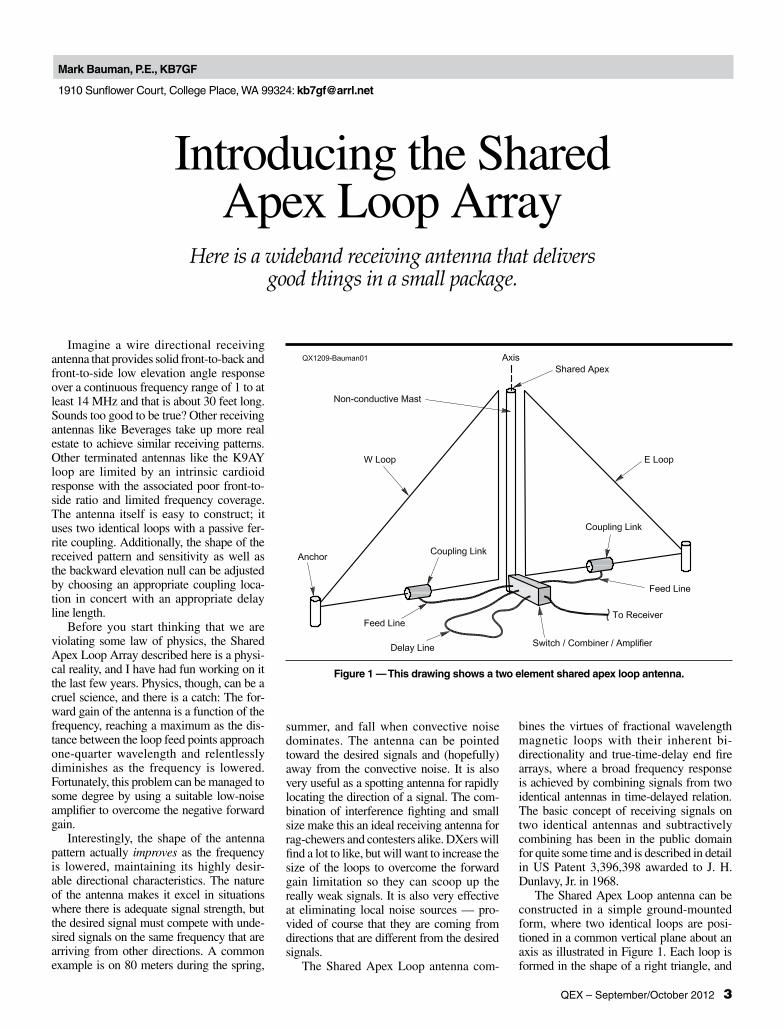
The Shared Apex Loop antenna can be constructed in a simple ground-mounted form, where two identical loops are posi-tioned in a common vertical plane about an axis as illustrated in Figure 1. Each loop is formed in the shape of a right triangle, and

Figure 1 — This drawing shows a two element shared apex loop antenna.

4 QEX – September/October 2012

each is positioned in mirrored relation about an axis sharing an apex at the top. A reason-able size for the loops is fifteen feet wide, fourteen feet high for a loop perimeter of a little less than 50 feet. A non-conductive mast is aligned along the axis and serves to support and separate the vertical leg of each loop. In practice, a separation of at least one inch is appropriate. Each loop is held in tension by an anchor at a height at least six inches from the ground.

Signals captured by each loop are trans-ferred to a feed line using a coupling link provided by a set of ferrite cores forming a current transformer.1 The feed lines are con-nected to the coupling link so that the signals from each loop are opposite in phase. The location of each coupler relative to the axis is designated as the feed point, and is an impor-tant parameter that will be discussed later in this article.

The feed lines that connect to each cou-pling link must be identical in length and character. In my experiments, I have used both coax and balanced lines for this task. My current preference is for balanced lines because they weigh less and are easier to manage, but they require a balun to convert to single-ended signals before running through the delay line.

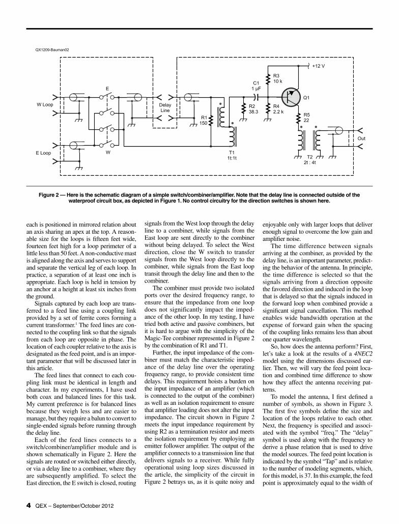
Each of the feed lines connects to a switch/combiner/amplifier module and is shown schematically in Figure 2. Here the signals are routed or switched either directly, or via a delay line to a combiner, where they are subsequently amplified. To select the East direction, the E switch is closed, routing

signals from the West loop through the delay line to a combiner, while signals from the East loop are sent directly to the combiner without being delayed. To select the West direction, close the W switch to transfer signals from the West loop directly to the combiner, while signals from the East loop transit through the delay line and then to the combiner.

The combiner must provide two isolated ports over the desired frequency range, to ensure that the impedance from one loop does not significantly impact the imped-ance of the other loop. In my testing, I have tried both active and passive combiners, but it is hard to argue with the simplicity of the Magic-Tee combiner represented in Figure 2 by the combination of R1 and T1.

Further, the input impedance of the com-biner must match the characteristic imped-ance of the delay line over the operating frequency range, to provide consistent time delays. This requirement hoists a burden on the input impedance of an amplifier (which is connected to the output of the combiner) as well as an isolation requirement to ensure that amplifier loading does not alter the input impedance. The circuit shown in Figure 2 meets the input impedance requirement by using R2 as a termination resistor and meets the isolation requirement by employing an emitter follower amplifier. The output of the amplifier connects to a transmission line that delivers signals to a receiver. While fully operational using loop sizes discussed in the article, the simplicity of the circuit in Figure 2 betrays us, as it is quite noisy and

enjoyable only with larger loops that deliver enough signal to overcome the low gain and amplifier noise.

The time difference between signals arriving at the combiner, as provided by the delay line, is an important parameter, predict-ing the behavior of the antenna. In principle, the time difference is selected so that the signals arriving from a direction opposite the favored direction and induced in the loop that is delayed so that the signals induced in the forward loop when combined provide a significant signal cancellation. This method enables wide bandwidth operation at the expense of forward gain when the spacing of the coupling links remains less than about one quarter wavelength.

So, how does the antenna perform? First, let’s take a look at the results of a 4NEC2 model using the dimensions discussed ear-lier. Then, we will vary the feed point loca-tion and combined time difference to show how they affect the antenna receiving pat-terns.

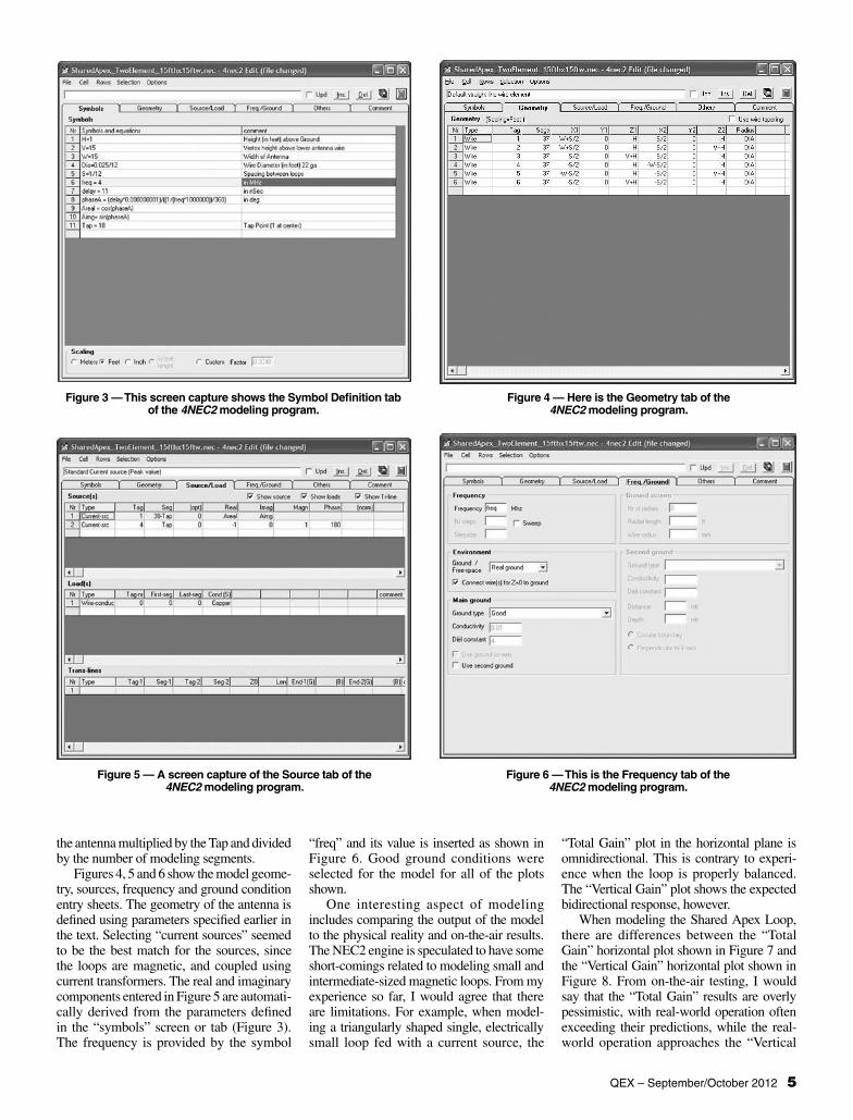
To model the antenna, I first defined a number of symbols, as shown in Figure 3. The first five symbols define the size and location of the loops relative to each other. Next, the frequency is specified and associ-ated with the symbol “freq.” The “delay” symbol is used along with the frequency to derive a phase relation that is used to drive the model sources. The feed point location is indicated by the symbol “Tap” and is relative to the number of modeling segments, which, for this model, is 37. In this example, the feed point is approximately equal to the width of

Figure 2 — Here is the schematic diagram of a simple switch/combiner/amplifier. Note that the delay line is connected outside of the waterproof circuit box, as depicted in Figure 1. No control circuitry for the direction switches is shown here.

QEX – September/October 2012 5

the antenna multiplied by the Tap and divided by the number of modeling segments.

Figures 4, 5 and 6 show the model geome-try, sources, frequency and ground condition entry sheets. The geometry of the antenna is defined using parameters specified earlier in the text. Selecting “current sources” seemed to be the best match for the sources, since the loops are magnetic, and coupled using current transformers. The real and imaginary components entered in Figure 5 are automati-cally derived from the parameters defined in the “symbols” screen or tab (Figure 3). The frequency is provided by the symbol

“freq” and its value is inserted as shown in Figure 6. Good ground conditions were selected for the model for all of the plots shown.

One interesting aspect of modeling includes comparing the output of the model to the physical reality and on-the-air results. The NEC2 engine is speculated to have some short-comings related to modeling small and intermediate-sized magnetic loops. From my experience so far, I would agree that there are limitations. For example, when model-ing a triangularly shaped single, electrically small loop fed with a current source, the

“Total Gain” plot in the horizontal plane is omnidirectional. This is contrary to experi-ence when the loop is properly balanced. The “Vertical Gain” plot shows the expected bidirectional response, however.

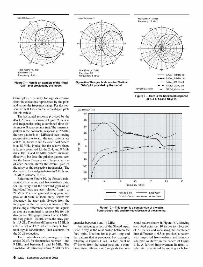
When modeling the Shared Apex Loop, there are differences between the “Total Gain” horizontal plot shown in Figure 7 and the “Vertical Gain” horizontal plot shown in Figure 8. From on-the-air testing, I would say that the “Total Gain” results are overly pessimistic, with real-world operation often exceeding their predictions, while the real-world operation approaches the “Vertical

Figure 3 — This screen capture shows the Symbol Definition tab of the 4NEC2 modeling program.

Figure 4 — Here is the Geometry tab of the 4NEC2 modeling program.

Figure 5 — A screen capture of the Source tab of the 4NEC2 modeling program.

Figure 6 — This is the Frequency tab of the 4NEC2 modeling program.

6 QEX – September/October 2012

Gain” plots especially for signals arriving from the elevations represented by the plots and across the frequency range. For this rea-son, we will focus on the vertical-gain plots for this article.

The horizontal response provided by the 4NEC2 model is shown in Figure 9 for sev-eral frequencies using a combined time dif-ference of 8 nanoseconds (ns). The innermost pattern is the horizontal response at 2 MHz; the next pattern is at 4 MHz and then moving progressively outward, the next patterns are at 8 MHz, 14 MHz and the outermost pattern is at 18 MHz. Notice that the relative shape is largely preserved for the 2, 4, and 8 MHz runs. The 14 and 18 MHz patterns maintain directivity but lose the pristine pattern seen for the lower frequencies. The relative size of each pattern shows the overall gain of the array at the respective frequencies. The decrease in forward gain between 2 MHz and 18 MHz is nearly 30 dB!

Referring to Figure 10, the forward gain, front-to-side ratio, and front-to-back ratio for the array and the forward gain of an individual loop are each plotted from 1 to 28 MHz. The loop gain and array gain both peak at 20 MHz, at about unity. Below this frequency, the array gain diverges from the loop gain as the frequency is lowered. The phase angle difference between the signals as they are combined is responsible for this divergence. The graph shows that at 1 MHz, the loop gain is –25 dBi, while the array gain is –45 dBi. The phase difference at 1 MHz is (180° – 3°) or 177°, which is only 3° from total signal cancellation. That accounts for the 20 dB reduction.

The front-to-back ratio manages to stay above 20 dB for frequencies between 1 and 9 MHz, and between 11 and 14 MHz. The Front-to-Side ratio stays above 20 dB for fre-

quencies between 1 and 14 MHz. An intriguing aspect of the Shared Apex

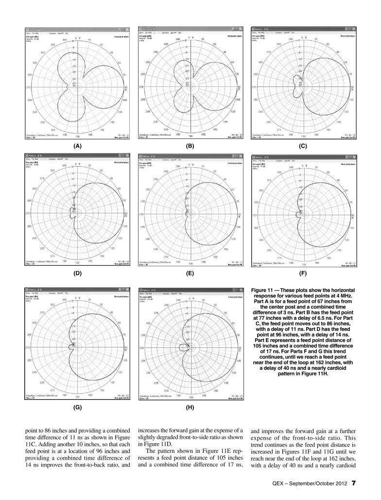
Loop Array is the relationship between the feed point location for a given loop and the pattern that it produces. For example, referring to Figures 11A-H, a feed point of 67 inches from the center post and a com-bined time difference of 3 ns yields the hori-

Figure 7 — Here is an example of the “Total Gain” plot provided by the model.

Figure 8 — This graph shows the “Vertical Gain” plot provided by the model.

Figure 9 — Here is the horizontal response at 2, 4, 8, 14 and 18 MHz.

Figure 10 — This graph is a comparison of the gain, front-to-back ratio and front-to-side ratio of the antenna.

zontal pattern shown in Figure 11A. Moving each feed point out 10 inches to a location of 77 inches and increasing the combined time difference to 6.5 ns provides a pattern with improved front-to-back and front-to-side ratio as shown in the pattern of Figure 11B. A further improvement in front-to-side ratio is achieved by moving each feed

QEX – September/October 2012 7

point to 86 inches and providing a combined time difference of 11 ns as shown in Figure 11C. Adding another 10 inches, so that each feed point is at a location of 96 inches and providing a combined time difference of 14 ns improves the front-to-back ratio, and

increases the forward gain at the expense of a slightly degraded front-to-side ratio as shown in Figure 11D.

The pattern shown in Figure 11E rep-resents a feed point distance of 105 inches and a combined time difference of 17 ns,

and improves the forward gain at a further expense of the front-to-side ratio. This trend continues as the feed point distance is increased in Figures 11F and 11G until we reach near the end of the loop at 162 inches, with a delay of 40 ns and a nearly cardioid

Figure 11 — These plots show the horizontal response for various feed points at 4 MHz. Part A is for a feed point of 67 inches from

the center post and a combined time difference of 3 ns. Part B has the feed point at 77 inches with a delay of 6.5 ns. For Part C, the feed point moves out to 86 inches, with a delay of 11 ns. Part D has the feed point at 96 inches, with a delay of 14 ns.

Part E represents a feed point distance of 105 inches and a combined time difference

of 17 ns. For Parts F and G this trend continues, until we reach a feed point

near the end of the loop at 162 inches, with a delay of 40 ns and a nearly cardioid

pattern in Figure 11H.

(A)

(D)

(G)

(B)

(E)

(H)

(C)

(F)

8 QEX – September/October 2012

pattern in Figure 11H. All of these patterns can be achieved simply by changing the com-bined time difference and moving the feed point. It should also be noted that the maxi-mum frequency for the array is a function of the time delay (tdiff). As a rule of thumb, the maximum effective frequency can be approximated by the following relation: fmax ≈ (1 / (5 × (tdiff)).

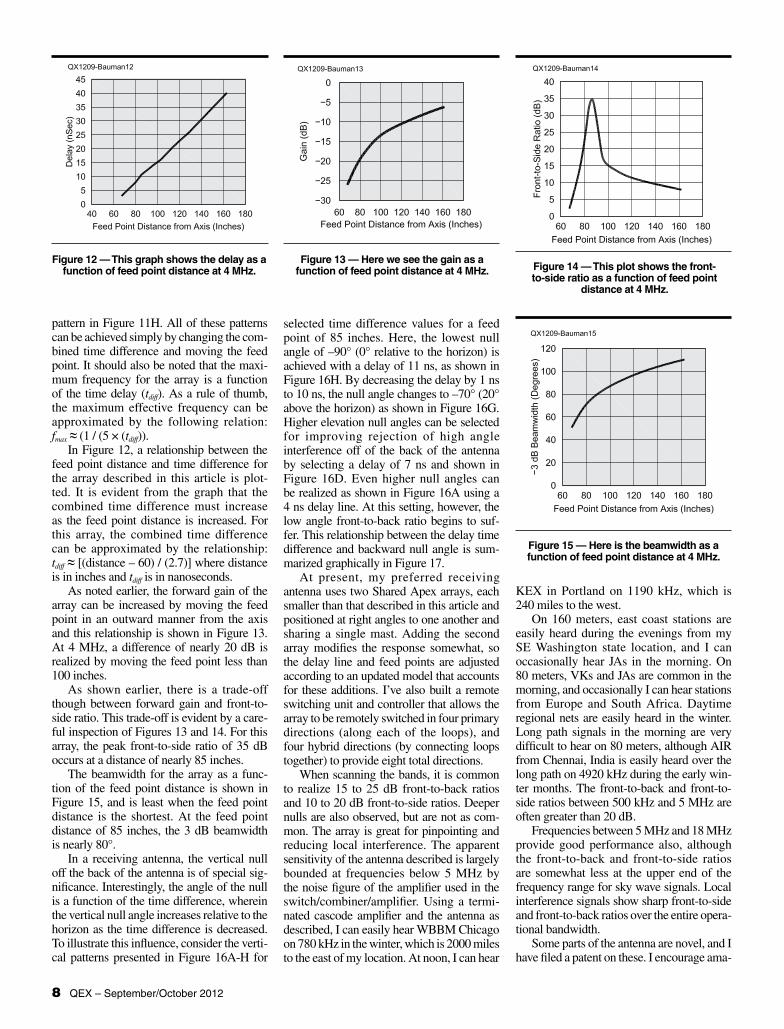
In Figure 12, a relationship between the feed point distance and time difference for the array described in this article is plot-ted. It is evident from the graph that the combined time difference must increase as the feed point distance is increased. For this array, the combined time difference can be approximated by the relationship: tdiff ≈ [(distance – 60) / (2.7)] where distance is in inches and tdiff is in nanoseconds.

As noted earlier, the forward gain of the array can be increased by moving the feed point in an outward manner from the axis and this relationship is shown in Figure 13. At 4 MHz, a difference of nearly 20 dB is realized by moving the feed point less than 100 inches.

As shown earlier, there is a trade-off though between forward gain and front-to-side ratio. This trade-off is evident by a care-ful inspection of Figures 13 and 14. For this array, the peak front-to-side ratio of 35 dB occurs at a distance of nearly 85 inches.

The beamwidth for the array as a func-tion of the feed point distance is shown in Figure 15, and is least when the feed point distance is the shortest. At the feed point distance of 85 inches, the 3 dB beamwidth is nearly 80°.

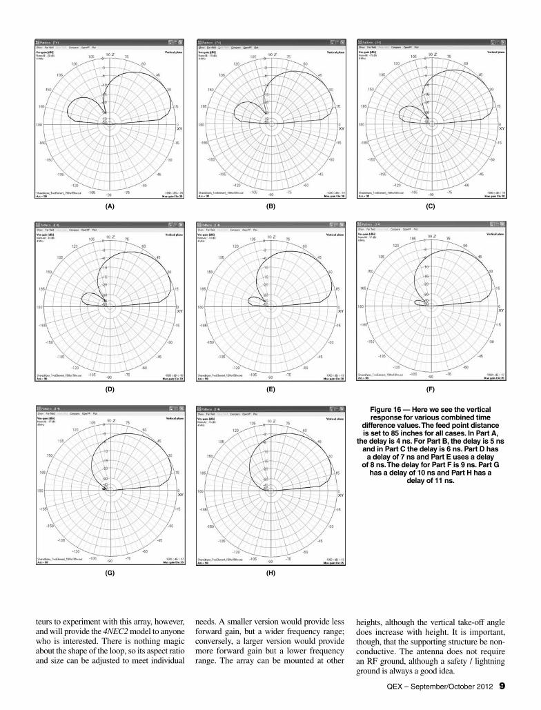
In a receiving antenna, the vertical null off the back of the antenna is of special sig-nificance. Interestingly, the angle of the null is a function of the time difference, wherein the vertical null angle increases relative to the horizon as the time difference is decreased. To illustrate this influence, consider the verti-cal patterns presented in Figure 16A-H for

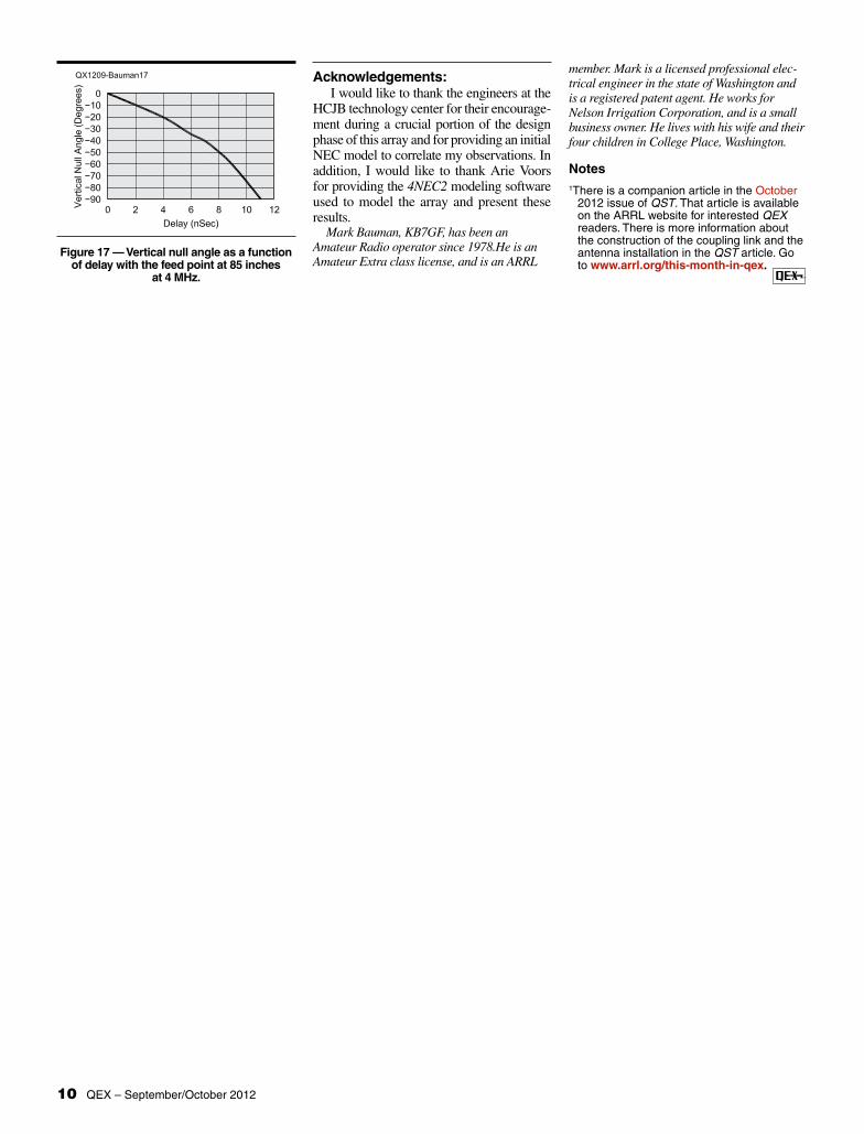
selected time difference values for a feed point of 85 inches. Here, the lowest null angle of –90° (0° relative to the horizon) is achieved with a delay of 11 ns, as shown in Figure 16H. By decreasing the delay by 1 ns to 10 ns, the null angle changes to –70° (20° above the horizon) as shown in Figure 16G. Higher elevation null angles can be selected for improving rejection of high angle interference off of the back of the antenna by selecting a delay of 7 ns and shown in Figure 16D. Even higher null angles can be realized as shown in Figure 16A using a 4 ns delay line. At this setting, however, the low angle front-to-back ratio begins to suf-fer. This relationship between the delay time difference and backward null angle is sum-marized graphically in Figure 17.

At present, my preferred receiving antenna uses two Shared Apex arrays, each smaller than that described in this article and positioned at right angles to one another and sharing a single mast. Adding the second array modifies the response somewhat, so the delay line and feed points are adjusted according to an updated model that accounts for these additions. I’ve also built a remote switching unit and controller that allows the array to be remotely switched in four primary directions (along each of the loops), and four hybrid directions (by connecting loops together) to provide eight total directions.

When scanning the bands, it is common to realize 15 to 25 dB front-to-back ratios and 10 to 20 dB front-to-side ratios. Deeper nulls are also observed, but are not as com-mon. The array is great for pinpointing and reducing local interference. The apparent sensitivity of the antenna described is largely bounded at frequencies below 5 MHz by the noise figure of the amplifier used in the switch/combiner/amplifier. Using a termi-nated cascode amplifier and the antenna as described, I can easily hear WBBM Chicago on 780 kHz in the winter, which is 2000 miles to the east of my location. At noon, I can hear

KEX in Portland on 1190 kHz, which is 240 miles to the west.

On 160 meters, east coast stations are easily heard during the evenings from my SE Washington state location, and I can occasionally hear JAs in the morning. On 80 meters, VKs and JAs are common in the morning, and occasionally I can hear stations from Europe and South Africa. Daytime regional nets are easily heard in the winter. Long path signals in the morning are very difficult to hear on 80 meters, although AIR from Chennai, India is easily heard over the long path on 4920 kHz during the early win-ter months. The front-to-back and front-to-side ratios between 500 kHz and 5 MHz are often greater than 20 dB.

Frequencies between 5 MHz and 18 MHz provide good performance also, although the front-to-back and front-to-side ratios are somewhat less at the upper end of the frequency range for sky wave signals. Local interference signals show sharp front-to-side and front-to-back ratios over the entire opera-tional bandwidth.

Some parts of the antenna are novel, and I have filed a patent on these. I encourage ama-

Figure 12 — This graph shows the delay as a function of feed point distance at 4 MHz.

Figure 13 — Here we see the gain as a function of feed point distance at 4 MHz. Figure 14 — This plot shows the front-

to-side ratio as a function of feed point distance at 4 MHz.

Figure 15 — Here is the beamwidth as a function of feed point distance at 4 MHz.

QEX – September/October 2012 9

(A)

(D)

(G)

(B)

(E)

(H)

(C)

(F)

Figure 16 — Here we see the vertical response for various combined time

difference values. The feed point distance is set to 85 inches for all cases. In Part A,

the delay is 4 ns. For Part B, the delay is 5 ns and in Part C the delay is 6 ns. Part D has

a delay of 7 ns and Part E uses a delay of 8 ns. The delay for Part F is 9 ns. Part G

has a delay of 10 ns and Part H has a delay of 11 ns.

teurs to experiment with this array, however, and will provide the 4NEC2 model to anyone who is interested. There is nothing magic about the shape of the loop, so its aspect ratio and size can be adjusted to meet individual

needs. A smaller version would provide less forward gain, but a wider frequency range; conversely, a larger version would provide more forward gain but a lower frequency range. The array can be mounted at other

heights, although the vertical take-off angle does increase with height. It is important, though, that the supporting structure be non-conductive. The antenna does not require an RF ground, although a safety / lightning ground is always a good idea.

10 QEX – September/October 2012

Acknowledgements:I would like to thank the engineers at the

HCJB technology center for their encourage-ment during a crucial portion of the design phase of this array and for providing an initial NEC model to correlate my observations. In addition, I would like to thank Arie Voors for providing the 4NEC2 modeling software used to model the array and present these results.

Mark Bauman, KB7GF, has been an Amateur Radio operator since 1978.He is an Amateur Extra class license, and is an ARRL

Figure 17 — Vertical null angle as a function of delay with the feed point at 85 inches

at 4 MHz.

member. Mark is a licensed professional elec-trical engineer in the state of Washington and is a registered patent agent. He works for Nelson Irrigation Corporation, and is a small business owner. He lives with his wife and their four children in College Place, Washington.

Notes1There is a companion article in the October

2012 issue of QST. That article is available on the ARRL website for interested QEX readers. There is more information about the construction of the coupling link and the antenna installation in the QST article. Go to www.arrl.org/this-month-in-qex.