Chapter 19: Decision Analysis 1

Chapter 19 Decision Analysis

LEARNING OBJECTIVES

Chapter 18 describes how to use decision analysis to improve management decisions, thereby enabling you to:

1. Learn about decision making under certainty, under uncertainty, and under risk. 2. Learn several strategies for decision-making under uncertainty, including

expected payoff, expected opportunity loss, maximin, maximax, and minimax regret.

3. Learn how to construct and analyze decision trees. 4. Understand aspects of utility theory. 5. Learn how to revise probabilities with sample information.

CHAPTER TEACHING STRATEGY

The notion of contemporary decision making is built into the title of the text as a statement of the importance of recognizing that statistical analysis is primarily done as a decision-making tool. For the vast majority of students, statistics take on importance only in as much as they aid decision-makers in weighing various alternative pathways and helping the manager make the best possible determination. It has been an underlying theme from chapter 1 that the techniques presented should be considered in a decision-making context. This chapter focuses on analyzing the decision-making situation and presents several alternative techniques for analyzing decisions under varying conditions.

Early in the chapter, the concepts of decision alternatives, the states of nature, and

the payoffs are presented. It is important that decision makers spend time brainstorming about possible decision alternatives that might be available to them. Sometimes the best alternatives are not obvious and are not immediately considered. The international focus

Chapter 19: Decision Analysis 2

on foreign companies investing in the U.S. presents a scenario in which there are several possible alternatives available. By using cases such as the Fletcher-Terry case at the chapter's end, students can practice enumerating possible decision alternatives.

States of nature are possible environments within which the outcomes will occur

over which we have no control. These include such things as the economy, the weather, health of the CEO, wildcat strikes, competition, change in consumer demand, etc. While the text presents problems with only a few states of nature in order to keep the length of solution reasonable, students should learn to consider as many states of nature as possible in decision making. Determining payoffs is relatively difficult but essential in the analysis of decision alternatives.

Decision-making under uncertainty is the situation in which the outcomes are not

known and there are no probabilities given as to the likelihood of them occurring. With these techniques, the emphasis is whether or not the approach is optimistic, pessimistic, or weighted somewhere in between.

In making decisions under risk, the probabilities of each state of nature occurring

are known or are estimated. Decision trees are introduced as an alternative mechanism for displaying the problem. The idea of an expected monetary value is that if this decision process were to continue with the same parameters for a long time, what would the long-run average outcome be? Some decisions lend themselves to long-run average analysis such as gambling outcomes or insurance actuary analysis. Other decisions such as building a dome stadium downtown or drilling one oil well tend to be more one time activities and may not lend themselves as nicely to expected value analysis. It is important that the student understand that expected value outcomes are long-run averages and probably will not occur in single instance decisions.

Utility is introduced more as a concept than an analytic technique. The

idea here is to aid the decision-maker in determining if he/she tends to be more of a risk-taker, an EMV'r, or risk-averse. The answer might be that it depends on the matter over which the decision is being made. One might be a risk-taker on attempting to employ a more diverse work force and at the same time be more risk-averse in investing the company's retirement fund.

Chapter 19: Decision Analysis 3

CHAPTER OUTLINE

19.1 The Decision Table and Decision Making Under Certainty

Decision Table Decision-Making Under Certainty

19.2 Decision Making Under Uncertainty Maximax Criterion Maximin Criterion Hurwicz Criterion Minimax Regret

19.3 Decision Making Under Risk

Decision Trees Expected Monetary Value (EMV) Expected Value of Perfect Information Utility

19.4 Revising Probabilities in Light of Sample Information

Expected Value of Sample Information

KEY TERMS

Decision Alternatives Hurwicz Criterion Decision Analysis Maximax Criterion Decision Making Under Certainty Maximin Criterion Decision Making Under Risk Minimax Regret Decision Making Under Uncertainty Opportunity Loss Table Decision Table Payoffs Decision Trees Payoff Table EMV'er Risk-Avoider Expected Monetary Value (EMV) Risk-Taker Expected Value of Perfect Information States of Nature Expected Value of Sample Information Utility

Chapter 19: Decision Analysis 4

SOLUTIONS TO PROBLEMS IN CHAPTER 19

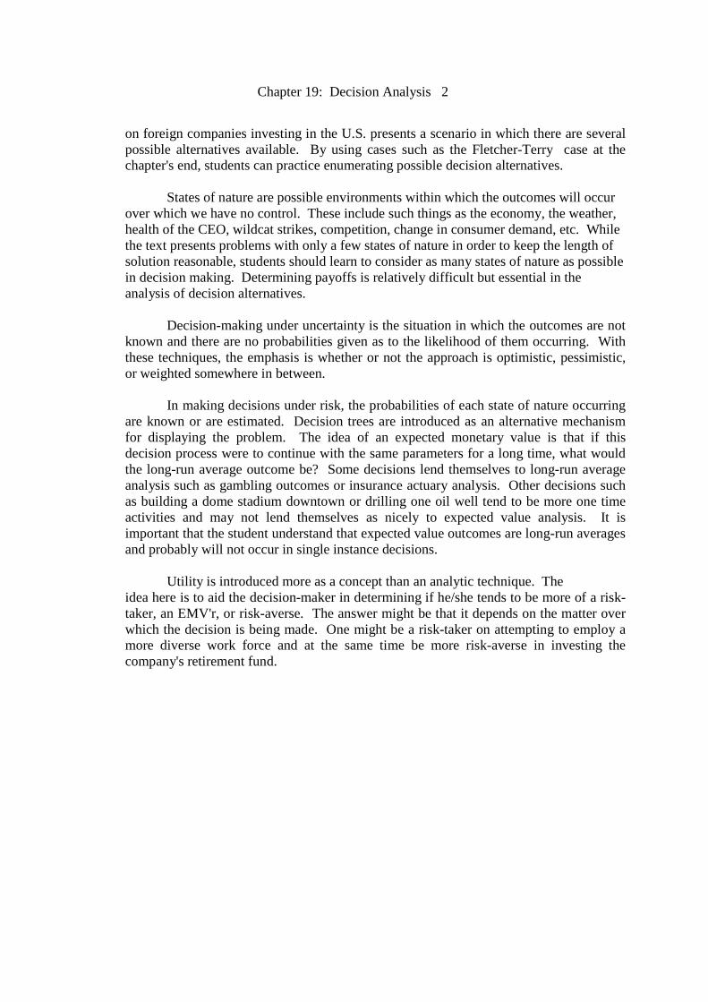
19.1 S1 S2 S3 Max Min d1 250 175 -25 250 -25 d2 110 100 70 110 70 d3 390 140 -80 390 -80 a.) Max {250, 110, 390} = 390 decision: Select d3 b.) Max {-25, 70, -80} = 70 decision: Select d2

c.) For α = .3 d1: .3(250) + .7(-25) = 57.5 d2: .3(110) + .7(70) = 82 d3: .3(390) + .7(-80) = 61 decision: Select d2 For α = .8 d1: .8(250) + .2(-25) = 195 d2: .8(110) + .2(70) = 102 d3: .8(390) + .2(-80) = 296 decision: Select d3

Comparing the results for the two different values of alpha, with a more pessimist point-of-view (α = .3), the decision is to select d2 and the payoff is 82. Selecting by using a more optimistic point-of-view (α = .8) results in choosing d3 with a higher payoff of 296.

Chapter 19: Decision Analysis 5

d.) The opportunity loss table is: S1 S2 S3 Max d1 140 0 95 140 d2 280 75 0 280 d3 0 35 150 150 The minimax regret = min {140, 280, 150} = 140 Decision: Select d1 to minimize the regret.

19.2 S1 S2 S3 S4 Max Min d1 50 70 120 110 120 50 d2 80 20 75 100 100 20 d3 20 45 30 60 60 20 d4 100 85 -30 -20 100 -30 d5 0 -10 65 80 80 -10 a.) Maximax = Max {120, 100, 60, 100, 80} = 120 Decision: Select d1 b.) Maximin = Max {50, 20, 20, -30, -10} = 50 Decision: Select d1 c.) α = .5 Max {[.5(120)+.5(50)], [.5(100)+.5(20)], [.5(60)+.5(20)], [.5(100)+.5(-30)], [.5(80)+.5(-10)]}= Max { 85, 60, 40, 35, 35 } = 85 Decision: Select d1

Chapter 19: Decision Analysis 6

d.) Opportunity Loss Table:November 8, 1996 S1 S2 S3 S4 Max d1 50 15 0 0 50 d2 20 65 45 10 65 d3 80 40 90 50 90 d4 0 0 150 130 150 d5 100 95 55 30 100 Min {50, 65, 90, 150, 100} = 50 Decision: Select d1

19.3 R D I Max Min A 60 15 -25 60 -25 B 10 25 30 30 10 C -10 40 15 40 -10 D 20 25 5 25 5 Maximax = Max {60, 30, 40, 25} = 60 Decision: Select A Maximin = Max {-25, 10, -10, 5} = 10 Decision: Select B

Chapter 19: Decision Analysis 7

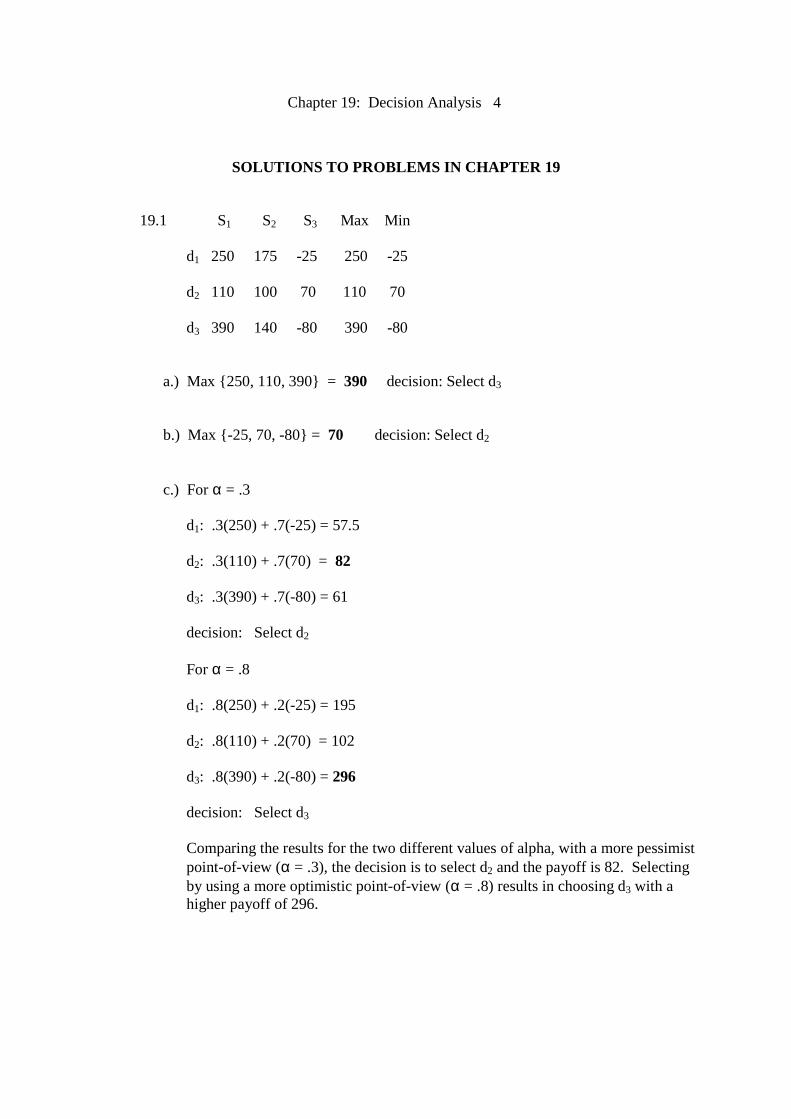
19.4 Not Somewhat Very Max Min

None -50 -50 -50 -50 -50 Few -200 300 400 400 -200 Many -600 100 1000 1000 -600 a.) For Hurwicz criterion using α = .6: Max {[.6(-50) + .4(-50)], [.6(400) + .4(-200)], [.6(1000) + .4(-600)]} = {-50, -160, 360}= 360 Decision: Select "Many" b.) Opportunity Loss Table: Not Somewhat Very Max None 0 350 1050 1050 Few 150 0 600 600 Many 550 200 0 550 Minimax regret = Min {1050, 600, 550} = 550 Decision: Select "Many"

Chapter 19: Decision Analysis 8

19.5, 19.6

Chapter 19: Decision Analysis 9

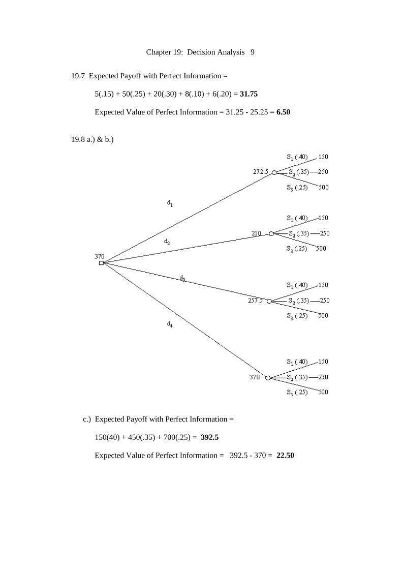
19.7 Expected Payoff with Perfect Information = 5(.15) + 50(.25) + 20(.30) + 8(.10) + 6(.20) = 31.75

Expected Value of Perfect Information = 31.25 - 25.25 = 6.50

19.8 a.) & b.)

c.) Expected Payoff with Perfect Information = 150(40) + 450(.35) + 700(.25) = 392.5 Expected Value of Perfect Information = 392.5 - 370 = 22.50

Chapter 19: Decision Analysis 10

19.9 Down(.30) Up(.65) No Change(.05) EMV

Lock-In -150 200 0 85 No 175 -250 0 -110 Decision: Based on the highest EMV)(85), "Lock-In" Expected Payoff with Perfect Information = 175(.30) + 200(.65) + 0(.05) = 182.5 Expected Value of Perfect Information = 182.5 - 85 = 97.5

19.10 EMV No Layoff -960 Layoff 1000 -320 Layoff 5000 400 Decision: Based on maximum EMV (400), Layoff 5000 Expected Payoff with Perfect Information = 100(.10) + 300(.40) + 600(.50) = 430 Expected Value of Perfect Information = 430 - 400 = 30

19.11 a.) EMV = 200,000(.5) + (-50,000)(.5) = 75,000 b.) Risk Avoider because the EMV is more than the investment (75,000 > 50,000) c.) You would have to offer more than 75,000 which is the expected value.

Chapter 19: Decision Analysis 11

19.12 a.) S1(.30) S2(.70) EMV d1 350 -100 35 d2 -200 325 167.5 Decision: Based on EMV, maximum {35, 167.5} = 167.5 b. & c.) For Forecast S1: Prior Cond. Joint Revised S1 .30 .90 .27 .6067 S2 .70 .25 .175 .3933 F(S1) = .445 For Forecast S2: Prior Cond. Joint Revised S1 .30 .10 .030 .054 S2 .70 .75 .525 .946 F(S2) = .555

Chapter 19: Decision Analysis 12

EMV with Sample Information = 241.63

d.) Value of Sample Information = 241.63 - 167.5 = 74.13

Chapter 19: Decision Analysis 13

19.13

Dec(.60) Inc(.40) EMV S -225 425 35 M 125 -150 15 L 350 -400 50 Decision: Based on EMV = Maximum {35, 15, 50} = 50 For Forecast (Decrease): Prior Cond. Joint Revised Decrease .60 .75 .45 .8824 Increase .40 .15 .06 .1176 F(Dec) = .51 For Forecast (Increase): Prior Cond. Joint Revised Decrease .60 .25 .15 .3061 Increase .40 .85 .34 .6939 F(Inc) = .49

Chapter 19: Decision Analysis 14

The expected value with sampling is 244.275

EVSI = EVWS - EMV = 244.275 - 50 = 194.275

Chapter 19: Decision Analysis 15

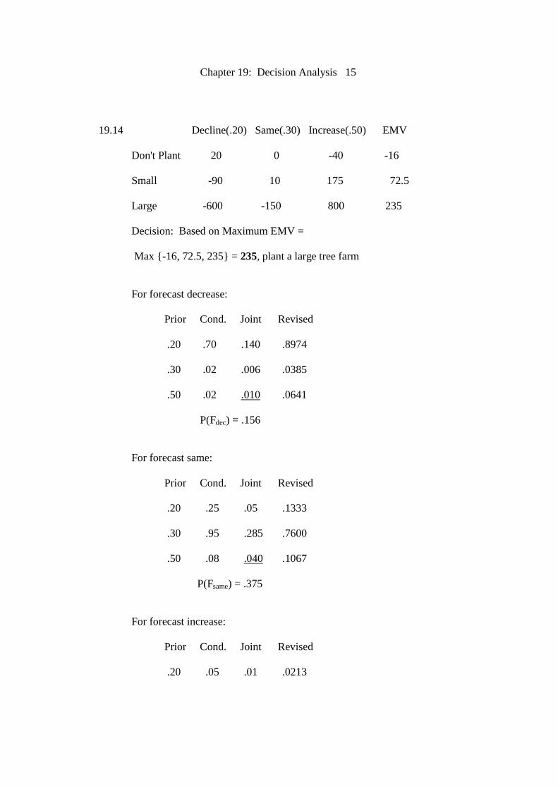
19.14 Decline(.20) Same(.30) Increase(.50) EMV Don't Plant 20 0 -40 -16 Small -90 10 175 72.5 Large -600 -150 800 235 Decision: Based on Maximum EMV = Max {-16, 72.5, 235} = 235, plant a large tree farm

For forecast decrease: Prior Cond. Joint Revised

.20 .70 .140 .8974 .30 .02 .006 .0385 .50 .02 .010 .0641 P(Fdec) = .156

For forecast same: Prior Cond. Joint Revised .20 .25 .05 .1333 .30 .95 .285 .7600 .50 .08 .040 .1067 P(Fsame) = .375

For forecast increase: Prior Cond. Joint Revised .20 .05 .01 .0213

Chapter 19: Decision Analysis 16

.30 .03 .009 .0192 .50 .90 .45 .9595 P(Finc) = .469

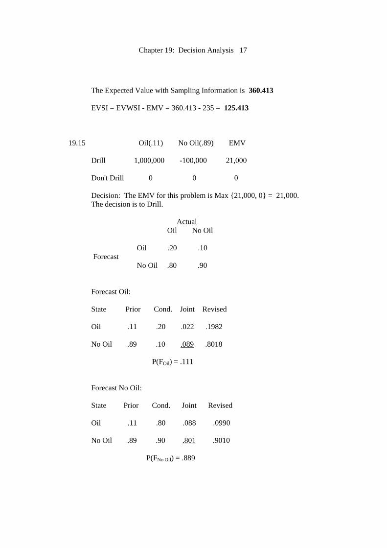
Chapter 19: Decision Analysis 17

The Expected Value with Sampling Information is 360.413 EVSI = EVWSI - EMV = 360.413 - 235 = 125.413

19.15 Oil(.11) No Oil(.89) EMV Drill 1,000,000 -100,000 21,000 Don't Drill 0 0 0 Decision: The EMV for this problem is Max {21,000, 0} = 21,000.

The decision is to Drill.

Actual Oil No Oil Oil .20 .10 Forecast No Oil .80 .90 Forecast Oil:

State Prior Cond. Joint Revised Oil .11 .20 .022 .1982 No Oil .89 .10 .089 .8018 P(FOil) = .111 Forecast No Oil: State Prior Cond. Joint Revised Oil .11 .80 .088 .0990 No Oil .89 .90 .801 .9010 P(FNo Oil) = .889

Chapter 19: Decision Analysis 18

The Expected Value With Sampling Information is 21,012.32 EVSI = EVWSI - EMV = 21,000 - 21,012.32 = 12.32

Chapter 19: Decision Analysis 19

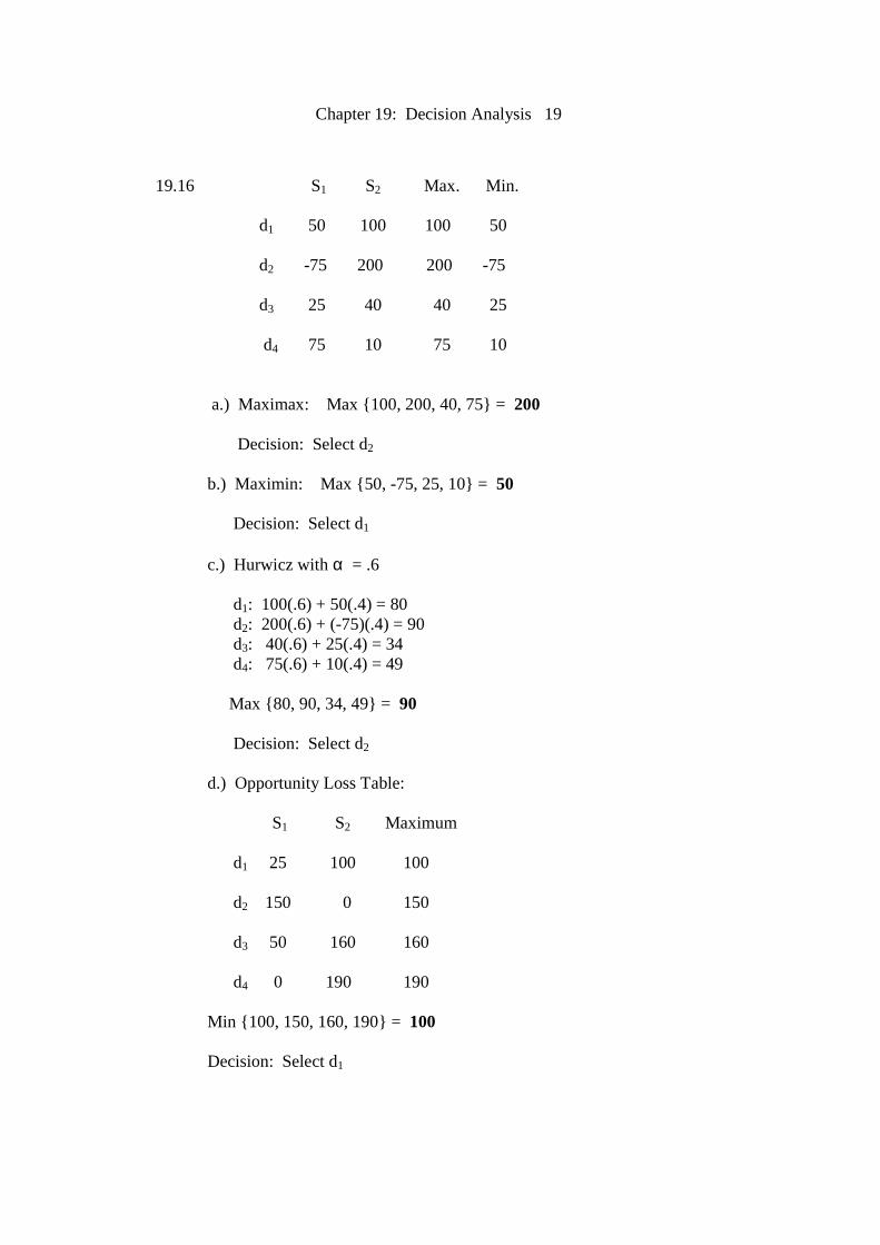
19.16 S1 S2 Max. Min.

d1 50 100 100 50 d2 -75 200 200 -75 d3 25 40 40 25 d4 75 10 75 10 a.) Maximax: Max {100, 200, 40, 75} = 200 Decision: Select d2 b.) Maximin: Max {50, -75, 25, 10} = 50 Decision: Select d1 c.) Hurwicz with α = .6 d1: 100(.6) + 50(.4) = 80 d2: 200(.6) + (-75)(.4) = 90 d3: 40(.6) + 25(.4) = 34 d4: 75(.6) + 10(.4) = 49 Max {80, 90, 34, 49} = 90 Decision: Select d2 d.) Opportunity Loss Table: S1 S2 Maximum d1 25 100 100 d2 150 0 150 d3 50 160 160 d4 0 190 190 Min {100, 150, 160, 190} = 100

Decision: Select d1

Chapter 19: Decision Analysis 20

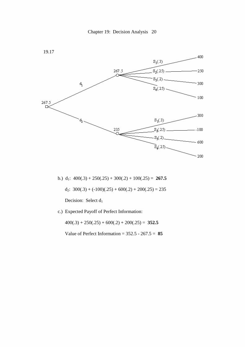
19.17

b.) d1: 400(.3) + 250(.25) + 300(.2) + 100(.25) = 267.5 d2: 300(.3) + (-100)(.25) + 600(.2) + 200(.25) = 235 Decision: Select d1 c.) Expected Payoff of Perfect Information: 400(.3) + 250(.25) + 600(.2) + 200(.25) = 352.5 Value of Perfect Information = 352.5 - 267.5 = 85

Chapter 19: Decision Analysis 21

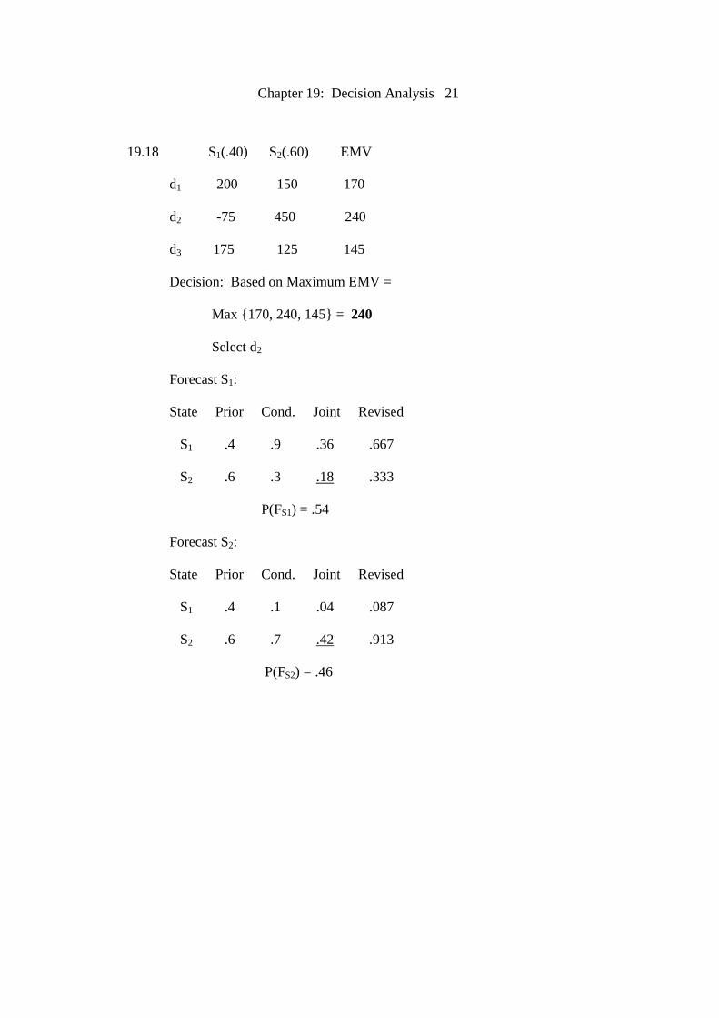
19.18 S1(.40) S2(.60) EMV

d1 200 150 170 d2 -75 450 240 d3 175 125 145 Decision: Based on Maximum EMV = Max {170, 240, 145} = 240 Select d2 Forecast S1: State Prior Cond. Joint Revised S1 .4 .9 .36 .667 S2 .6 .3 .18 .333 P(FS1) = .54 Forecast S2: State Prior Cond. Joint Revised S1 .4 .1 .04 .087 S2 .6 .7 .42 .913 P(FS2) = .46

Chapter 19: Decision Analysis 22

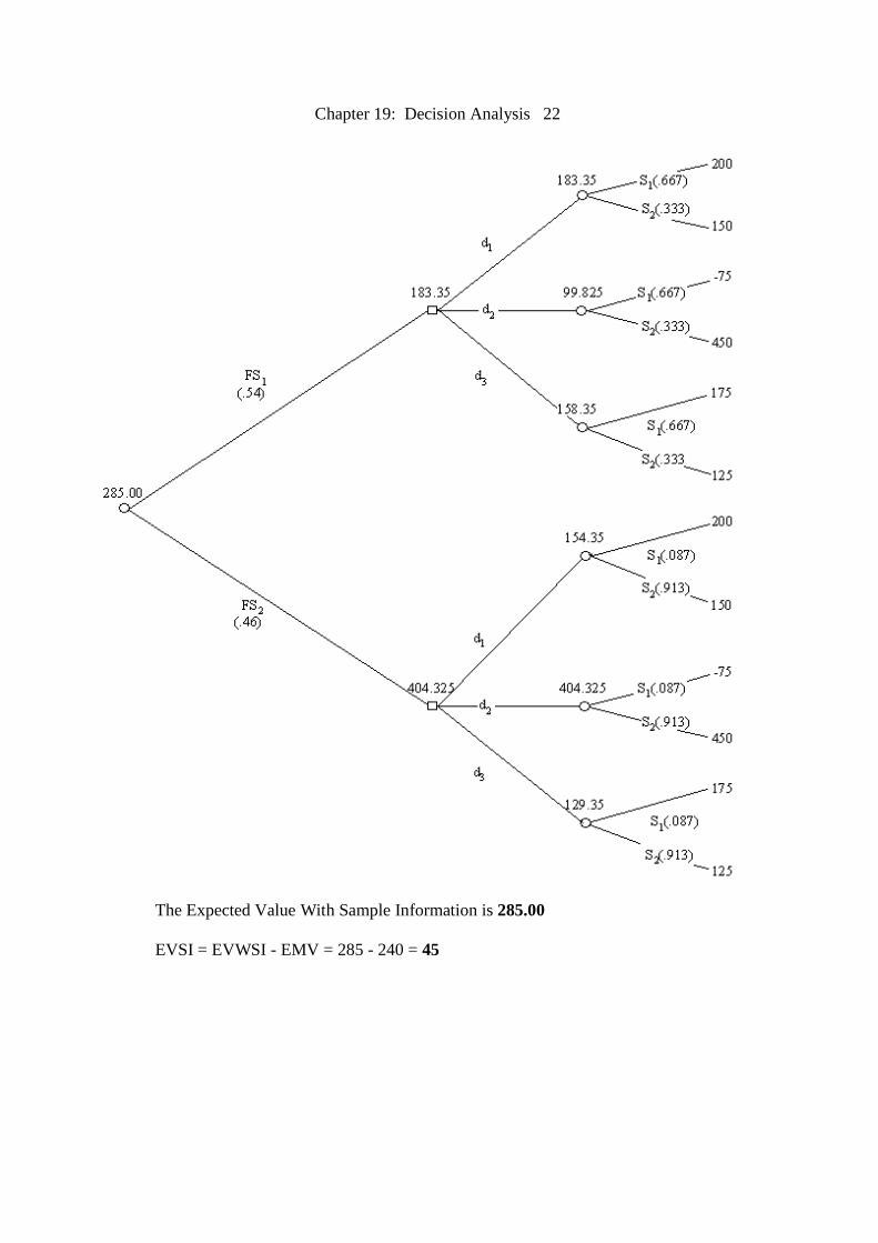
The Expected Value With Sample Information is 285.00

EVSI = EVWSI - EMV = 285 - 240 = 45

Chapter 19: Decision Analysis 23

19.19 Small Moderate Large Min Max

Small 200 250 300 200 300 Modest 100 300 600 100 600 Large -300 400 2000 -300 2000 a.) Maximax: Max {300, 600, 2000} = 2000 Decision: Large Number Minimax: Max {200, 100, -300} = 200 Decision: Small Number b.) Opportunity Loss: Small Moderate Large Max Small 0 150 1700 1700 Modest 100 100 1400 1400 Large 500 0 0 500 Min {1700, 1400, 500} = 500 Decision: Large Number c.) Minimax regret criteria leads to the same decision as Maximax.

Chapter 19: Decision Analysis 24

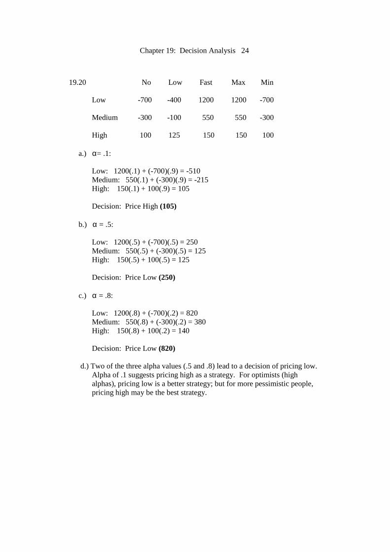
19.20 No Low Fast Max Min

Low -700 -400 1200 1200 -700 Medium -300 -100 550 550 -300 High 100 125 150 150 100 a.) α= .1: Low: 1200(.1) + (-700)(.9) = -510 Medium: 550(.1) + (-300)(.9) = -215 High: 150(.1) + 100(.9) = 105 Decision: Price High (105)

b.) α = .5: Low: 1200(.5) + (-700)(.5) = 250 Medium: 550(.5) + (-300)(.5) = 125 High: 150(.5) + 100(.5) = 125 Decision: Price Low (250) c.) α = .8: Low: 1200(.8) + (-700)(.2) = 820 Medium: 550(.8) + (-300)(.2) = 380 High: 150(.8) + 100(.2) = 140 Decision: Price Low (820)

d.) Two of the three alpha values (.5 and .8) lead to a decision of pricing low. Alpha of .1 suggests pricing high as a strategy. For optimists (high alphas), pricing low is a better strategy; but for more pessimistic people, pricing high may be the best strategy.

Chapter 19: Decision Analysis 25

19.21 Mild(.75) Severe(.25) EMV Reg. 2000 -2500 875 Weekend 1200 -200 850 Not Open -300 100 -200 Decision: Based on Max EMV = Max{875, 850, -200} = 875, open regular hours.

Expected Value with Perfect Information = 2000(.75) + 100(.25) = 1525 Value of Perfect Information = 1525 - 875 = 650

Chapter 19: Decision Analysis 26

19.22 Weaker(.35) Same(.25) Stronger(.40) EMV

Don't Produce -700 -200 150 -235 Produce 1800 400 -1600 90 Decision: Based on Max EMV = Max {-235, 90} = 90, select Produce. Expected Payoff With Perfect Information = 1800(.35) + 400(.25) + 150(.40) = 790

Value of Perfect Information = 790 - 90 = 700

Chapter 19: Decision Analysis 27

19.23 Red.(.15) Con.(.35) Inc.(.50) EMV Automate -40,000 -15,000 60,000 18,750 Do Not 5,000 10,000 -30,000 -10,750 Decision: Based on Max EMV = Max {18750, -10750} = 18,750, Select Automate Forecast Reduction: State Prior Cond. Joint Revised R .15 .60 .09 .60 C .35 .10 .035 .2333 I .50 .05 .025 .1667 P(FRed) = .150 Forecast Constant: State Prior Cond. Joint Revised R .15 .30 .045 .10 C .35 .80 .280 .6222 I .50 .25 .125 .2778 P(FCons) = .450

Forecast Increase:

State Prior Cond. Joint Revised

R .15 .10 .015 .0375 C .35 .10 .035 .0875 I .50 .70 .350 .8750 P(FInc) = .400

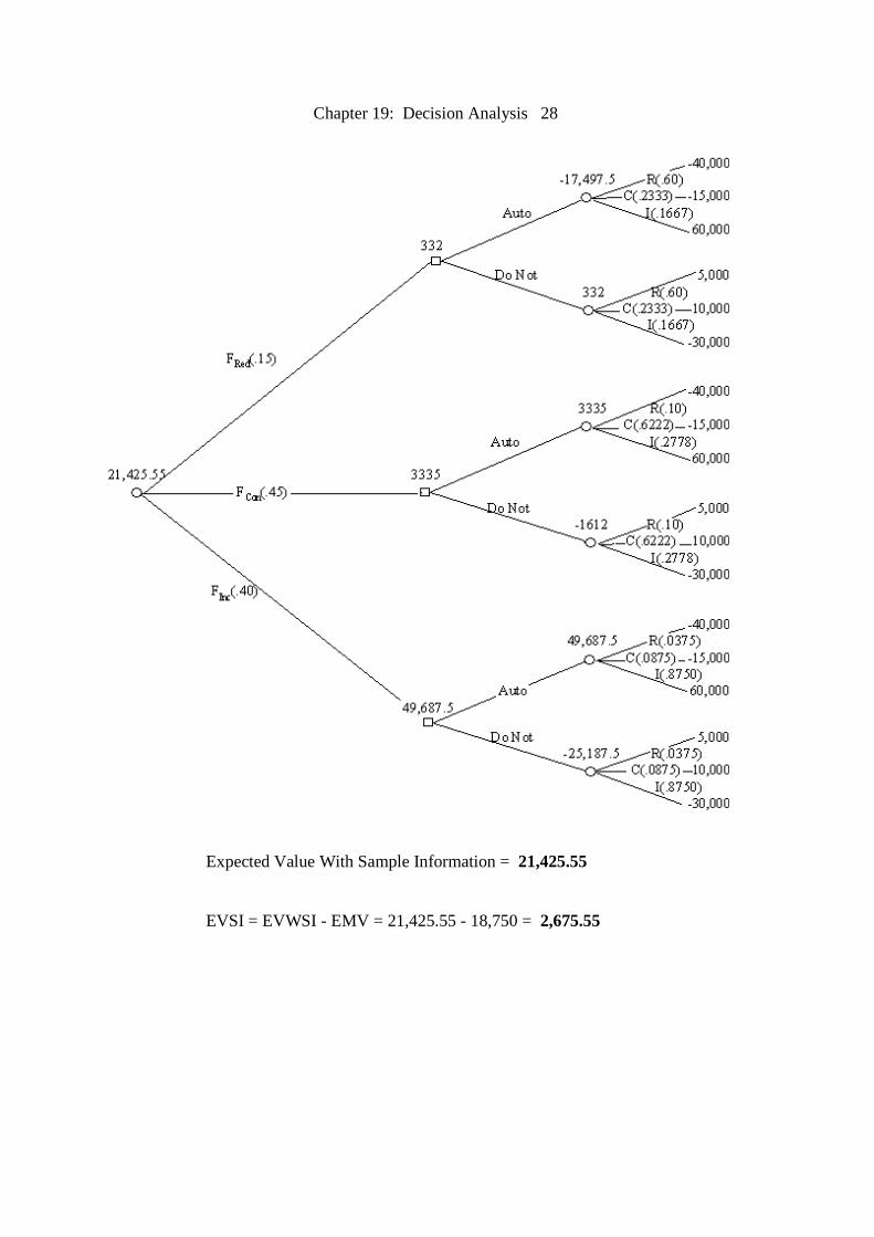
Chapter 19: Decision Analysis 28

Expected Value With Sample Information = 21,425.55 EVSI = EVWSI - EMV = 21,425.55 - 18,750 = 2,675.55

Chapter 19: Decision Analysis 29

19.24 Chosen(.20) Not Chosen(.80) EMV Build 12,000 -8,000 -4,000 Don't -1,000 2,000 1,400 Decision: Based on Max EMV = Max {-4000, 1400} = 1,400, choose "Don't Build" as a strategy. Forecast Chosen: State Prior Cond. Joint Revised Chosen .20 .45 .090 .2195 Not Chosen .80 .40 .320 .7805 P(FC) = .410 Forecast Not Chosen: State Prior Cond. Joint Revised Chosen .20 .55 .110 .1864 Not Chosen .80 .60 .480 .8136 P(FC) = .590

Chapter 19: Decision Analysis 30

Expected Value With Sample Information = 1,400.09

EVSI = EVWSI - EMV = 1,400.09 - 1,400 = .09