Discussion Papers

Inequality over the Business Cycle – The Role of Distributive Shocks

Marius Clemens, Ulrich Eydam, Maik Heinemann

1852

Deutsches Institut für Wirtschaftsforschung 2020

Opinions expressed in this paper are those of the author(s) and do not necessarily reflect views of the institute.

IMPRESSUM

© DIW Berlin, 2020

DIW Berlin German Institute for Economic Research Mohrenstr. 58 10117 Berlin

Tel. +49 (30) 897 89-0 Fax +49 (30) 897 89-200 http://www.diw.de

ISSN electronic edition 1619-4535

Papers can be downloaded free of charge from the DIW Berlin website: http://www.diw.de/discussionpapers

Discussion Papers of DIW Berlin are indexed in RePEc and SSRN: http://ideas.repec.org/s/diw/diwwpp.html http://www.ssrn.com/link/DIW-Berlin-German-Inst-Econ-Res.html

Inequality over the Business Cycle - The Role of Distributive

Shocks

Marius Clemens (DIW Berlin, BERA), Ulrich Eydam (University of Potsdam),Maik Heinemann (University of Potsdam)

February 13, 2020

This paper examines the dynamics of wealth and income inequality along the

business cycle and assesses how they are related to fluctuations in the functional

income distribution. In a panel estimation for OECD countries between 1970 and

2016 we find that on average income inequality - measured by the Gini coefficient - is

countercyclical and also shows a significant association with the capital share. Up on a

closer look, we find that a remarkable share of one third of all countries display a rather

pro- or acyclical relationship. In order to understand the underlying cyclical dynamics

of inequality we incorporate distributive shocks, modeled as exogenous changes in the

capital share, into a real business cycle model, where agents are ex-ante heterogeneous

with respect to wealth and ability. We show how to derive standard inequality measures

within this framework, which allow us to analyze how productivity and distributive

shocks affect both, the macroeconomic variables and the personal income and wealth

distribution over the business cycle.

We find that whether wealth and income inequality in the model behaves counter-

cyclical or not depends on two aspects. The intertemporal elasticity of substitution

and the persistence of the shocks. We use Bayesian techniques in order to match GDP,

capital share and consumption to quarterly U.S. data. The resulting parameter estimates

point towards a non-monotonic relationship between productivity fluctuations and

inequality. On impact, inequality increases in response to TFP shocks but declines

in later periods. This pattern is consistent with the empirically observed relationship

in the USA. Furthermore, we find that TFP shocks explain about 17 percent of the

cyclical fluctuations in inequality in the USA.

JEL-Classification: D31, E25, E32

Keywords: Business Cycle, Income and Wealth Inequality, Distributive Shocks

1 Introduction

In economics, the relationship between inequality and economic growth is controversially debated.

Many studies concentrate on the long-term effects from inequality on growth or vice versa. Although

surely a substantial amount of changes in the income and wealth distribution can be accounted

for by structural changes, short term business cycle-related changes also have non-neglectable

distributional effects: In recessions or booms income and wealth of specific-income groups will not

grow symmetrically. For example, during a recession, households at the lower end of the income

and wealth distributions are more negatively affected when becoming unemployed. This would

make the income distribution rather countercyclical. In contrast, rich households who hold large

parts of the capital stock face high capital income losses, which would rather lead to procyclical

distributional dynamics. Therefore, it is a priori unclear how inequality behaves over the business

cycle.

A large part of the current debate concentrates on trends for wealth and income inequality that

are identified from the relevant data, see for example Alvaredo et al. (2017). Given the fact that the

underlying statistics are still capable of development, in particular, we lack satisfactory statistics

regarding the wealth distribution, and for both wealth as well as income inequality time series with

a high periodicity even for the more recent past are missing, the business cycle perspective might be

of some interest too. In order to assess the empirical evidence regarding the evolution of inequality

and to discuss supposed structural causes, it is certainly helpful to know to what extent the recent

trends in inequality can be attributed to business cycle dynamics or are truly the result of structural

changes.

Recent studies use complex ex-ante heterogeneous-agent models (HAM, HANK) in order to

analyze the interactions between inequality and the macroeconomy (Kaplan and Violante (2018),

Ahn et al. (2017)). They focus on distributional effects of fiscal and monetary policies (Kaplan et al.

(2018), Ragot and Grand (2017), Bayer and Luetticke (2018)) and also the causes and consequences

of increasing income and wealth inequality in the U.S. (Kuhn et al. (2019), Bayer and Luetticke

(2019)). There are also papers that try to reduce the complexity of heterogeneous agent models,

i.e by using two agent, but still catch relevant part of the macro-inequality relationship (Iacoviello

(2005), Galı et al. (2007), Challe et al. (2017), Debortoli and Galı (2017)). Clearly, analyzing

the macro-inequality nexus within a full-fledged HANK model can and should not be replaced

them. However, simplifying the macro-inequality relationship can provide stylized results which

are testable with state-of-the art estimation methods (i.e. Bayesian estimation). Furthermore, the

model can be used as approximation to get an impression to what extend inequality and the business

cycle are related. Our paper contributes to this strand of literature by providing a simplified way to

incorporate income and wealth inequality measures in a real business cycle model with TFP and

distributive shocks.

Another topic, that has been discussed extensively in recent times are trends and fluctuations

in the functional income distribution, i.e. changes in the capital and labor share. As documented

by Growiec et al. (2018), functional income shares display a long run trend and fluctuate at

business cycle frequencies. Rıos-Rull and Santaeulalia-Llopis (2010), Mangin and Sedlacek

1

(2018) and Cantore et al. (2018) highlight that these fluctuations are linked to fluctuations in

macroeconomic aggregates and have important implications for macroeconomic dynamics. As

discussed by Atkinson (2009) it seems natural to expect that the functional income distribution is

linked to the personal income distribution. Lansing (2015) incorporates persistent changes in the

functional income distribution into a macro-model, in order to analyze the long-term development

of the equity premium. Yet, how business cycle fluctuations in the functional income distribution

are related to fluctuations in the personal income distribution has not been examined. In the present

paper, we aim to fill this gap in the literature and provide an account of the cyclical properties of

the personal and functional income distribution and their dynamic relationship.

In order to better understand short run inequality dynamics and the distributional consequences

of oscillations in income shares, we proceed in two ways. First, we examine the cyclical correlation

between GDP, the capital share and the Gini coefficient of the income distribution in a panel of

OECD countries for the period between 1970 and 2017. The results of the panel regressions show

that on average, the relationship between cyclical fluctuations in GDP and the Gini coefficient is

statistically significant and countercyclical. Furthermore, the results also point towards a significant

link between the functional and personal income distributions. However, a closer look at the

contemporaneous correlations between the cyclical components reveals substantial heterogeneity

across countries, i.e. roughly one third of countries in the sample, including the United States, show

a rather procyclical or at least acyclical relationship between inequality and GDP. In a detailed

examination of the cyclical relationships for the United States, we find that the Gini coefficient of

the income distribution and the capital share are about one third as volatile as GDP. Furthermore,

we observe a switching sign after around one year in the cross-correlations between GDP and the

Gini coefficient.

Therefore, in a second step, we employ a real business cycle model with agents that differ with

respect to their initial productivity and wealth endowments following the approach of Maliar et al.

(2005).1 We use this framework and derive analytical expressions for several standard inequality

measures which define the dynamics of the cross section in terms of aggregate variables. We put

particular emphasize on the assumptions that are necessary for this derivation and discuss their

implications regarding possible applications. In order to understand the role of cyclical variation

in factor income shares and inspired by work of Young (2004), Rıos-Rull and Santaeulalia-Llopis

(2010) and Lansing (2015), we add distributive shocks to the model. Given the theoretical model,

we show that the cyclicality of inequality depends crucially on the intertemporal elasticity of

substitution and the shape of the stochastic process that induce aggregate dynamics.

Finally, to in order to test the theoretical predictions from our model and to match the theoretical

considerations with the empirical findings, we use Bayesian methods and estimate the model, using

data for the United States.2 In the light of the theoretical discussion, the estimated parameter values

1This approach builds on previous work in this respect by Chatterjee (1994) and Caselli and Ventura (2000), whoexamine inequality in a deterministic context. For a discussion of the model in a stochastic environment also seeMaliar and Maliar (2001).

2The ability to estimate the model is one advantage of the approach presented here. In contrast to models with ex-postheterogeneity, which results from incomplete markets, as for example in Aiyagari (1994), the present model canbe solved via perturbation and admits a compact state space representation that is easily suitable for estimation via

2

suggest a procyclical relationship between inequality measures and GDP. This is also confirmed

by the respective impulse responses, where we observe that inequality increases in response to

TFP and distributive shocks. However, while the initial response of inequality measures to a TFP

shock is positive, inequality starts to decline during the subsequent periods, i.e. the relationship

turns countercyclical in the medium term. Thus, the estimated model is also able to replicate the

negative sign of lagged cross-correlations between the cyclical components of inequality measures

and GDP, observed for the United States. According to a variance decomposition of the empirical

model, about 85% of the cyclical fluctuations in inequality measures in the United States result

from distributive shocks. So overall, our results suggest that the observed differences in the

cyclical relationship between inequality measures and GDP across countries can be traced back to

differences in structural parameters and distinct causes of cyclical fluctuations. Furthermore, our

analysis reveals the important role of distributive shocks for short run inequality dynamics.

The remainder of this paper is structured as follows. The second section presents the empirical

findings for the group of OECD countries and the analysis of the cyclical properties of inequality

measures, GDP and the capital share. The third section presents the theoretical model and the

derivation of inequality measures. The fourth section discusses the models implications regarding

the relationship between inequality and productivity shocks, as well as distributive shocks. Further-

more, it presents the results of matching the model to U.S. data and assesses the models ability to

replicate empirical facts. The fifth section concludes.

2 Inequality and the Business Cycle: Empirical facts

2.1 OECD Panel Comparison

We start with a general assessment of the relationship between inequality and the business cycle. In

the first step we estimate a panel fixed-effects model based on annual data between 1970 and 2016

in order to highlight the relationship between the state of the business cycle and inequality in OECD

countries. Thereby we follow existing studies in explaining income inequality measured by the

Gini coefficient of net disposable income.3 As main determinant of income inequality we consider

GDP per capita, the squared GDP per capita and the degree of openness. Since we are interested

in the relationship between inequality and the business cycle, we also consider the business cycle

measured by the HP-filtered GDP series.4 Furthermore, to assess the relationship between the

functional income distribution and the Gini coefficient, we include the cyclical component of the

capital share. Inequality data were drawn from the UNU-WIDER Database, the data series for

the macroeconomic variables stem from the Penn World Tables 9.0, as described in Feenstra et al.

(2015).

Bayesian methods.3See Barro (2000) for a comprehensive analysis. Since we concentrate on OECD countries, we do not control for

colonies, political system and region specific dummies.4We considered a smoothing parameter of 6.25. Business cycle data are introduced with a delay of one period as

predetermined, to reduce the influence of reverse causality by assumption. We also conduct robustness analysis withdifferent time periods, smoothing parameters and filtering methods (Bandpass filter, Hamilton Filter), but our resultsdo not change quantitatively.

3

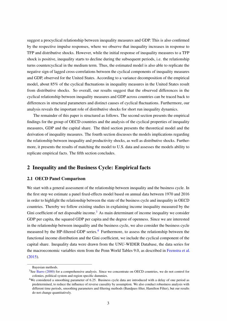
Gini coefficient after redistr. before redistr.

GDP pc log -4.33*** -4.96***GDP pc squared 0.09*** 0.11***Business Cyclet−1×100 -0.10* -0.20***Capital share cyclet−1×100 0.30** 0.30***Openess ×100 -3.40 0.80

R-squared 0.25 0.51Obs 966 966Country FE Y Y∗ denotes 90%-Significance-Level, ∗∗ denotes 95%-Significance-Level and ∗∗∗ de-

notes 97.5%-Significance-Level. The Gini Coefficient after redistribution is the netGini coefficient of disposable household income. Before redistribution it is the Ginicoefficient of market income.

Table 1: The relationship between income inequality and the business cycle - OECD countries,1970 – 2017

Our baseline estimation, presented in table 1, confirms results from previous studies:5 Ne-

glecting low and medium-income Non-OECD countries in the estimation cuts off the first part

of the Kutznets curve, such that we observe a U-shaped relationship between income inequality

and GDP per capita. Openness is positively correlated with income inequality but not statistically

significant, mostly because openness in OECD countries does not vary much between countries.

However, the business cycle of OECD countries, as measured by the cyclical component of GDP, is

on average negatively and significantly correlated with income inequality. Although we estimate

correlations, our results suggest that in a boom situation, income inequality may shrink, while

recessions could lead to increases in income inequality. For cyclical variations in the functional

income distribution, we detect a positive and statistically significant correlation. This indicates

that increases in the capital share are on average associated with rising inequality. Finally, by

comparing income inequality over the cycle before and after redistribution policy, we find that

the relationship between business cycles and income inequality becomes less countercyclical after

redistribution policies. This could be a sign for the effectiveness of automatic cyclical stabilizers,

i.e. unemployment benefits or income tax in specific countries.6

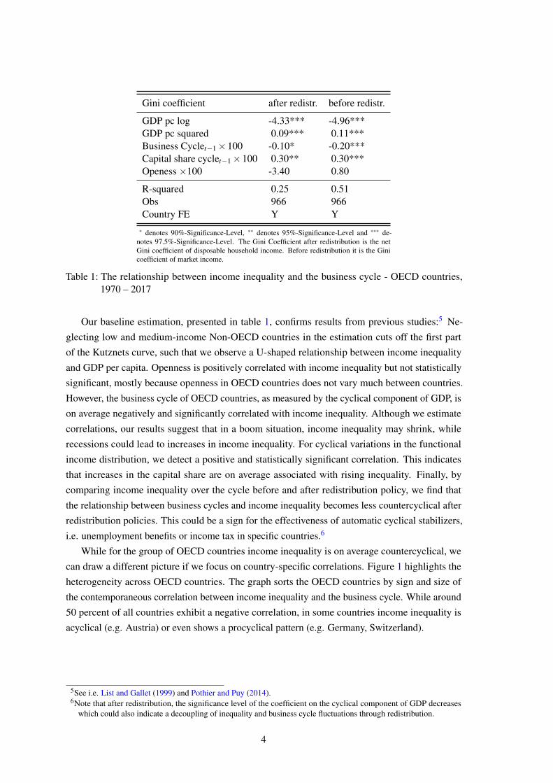
While for the group of OECD countries income inequality is on average countercyclical, we

can draw a different picture if we focus on country-specific correlations. Figure 1 highlights the

heterogeneity across OECD countries. The graph sorts the OECD countries by sign and size of

the contemporaneous correlation between income inequality and the business cycle. While around

50 percent of all countries exhibit a negative correlation, in some countries income inequality is

acyclical (e.g. Austria) or even shows a procyclical pattern (e.g. Germany, Switzerland).

5See i.e. List and Gallet (1999) and Pothier and Puy (2014).6Note that after redistribution, the significance level of the coefficient on the cyclical component of GDP decreases

which could also indicate a decoupling of inequality and business cycle fluctuations through redistribution.

4

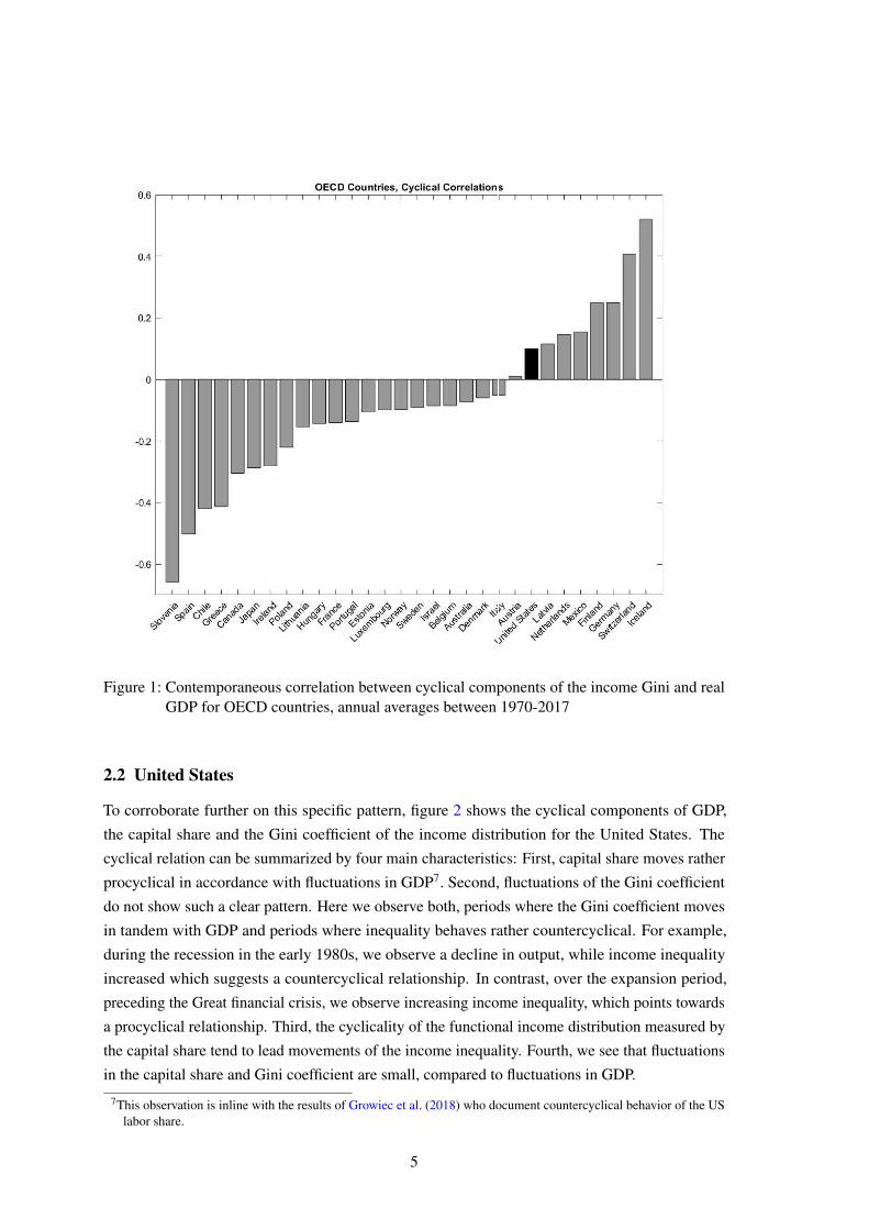
Figure 1: Contemporaneous correlation between cyclical components of the income Gini and realGDP for OECD countries, annual averages between 1970-2017

2.2 United States

To corroborate further on this specific pattern, figure 2 shows the cyclical components of GDP,

the capital share and the Gini coefficient of the income distribution for the United States. The

cyclical relation can be summarized by four main characteristics: First, capital share moves rather

procyclical in accordance with fluctuations in GDP7. Second, fluctuations of the Gini coefficient

do not show such a clear pattern. Here we observe both, periods where the Gini coefficient moves

in tandem with GDP and periods where inequality behaves rather countercyclical. For example,

during the recession in the early 1980s, we observe a decline in output, while income inequality

increased which suggests a countercyclical relationship. In contrast, over the expansion period,

preceding the Great financial crisis, we observe increasing income inequality, which points towards

a procyclical relationship. Third, the cyclicality of the functional income distribution measured by

the capital share tend to lead movements of the income inequality. Fourth, we see that fluctuations

in the capital share and Gini coefficient are small, compared to fluctuations in GDP.

7This observation is inline with the results of Growiec et al. (2018) who document countercyclical behavior of the USlabor share.

5

Figure 2: Cyclical components of real GDP, income Gini and capital share for the United States1970 – 2016.

This general pattern is also confirmed by the respective statistics presented in table 2. The

upper panel shows the standard deviation of the cyclical components for all three variables. Here

we see that the variation in Gini coefficients and capital shares amounts to roughly one third

of the variation in GDP, indicating that cyclical movements in inequality are less pronounced

compared to GDP fluctuations. The lower panel shows the cross-correlations for the cyclical

components of the Gini coefficient and GDP. We find a small positive contemporaneous correlation

between GDP fluctuations and fluctuations in the Gini coefficients of the income distribution. This

finding contrasts with the findings of Dimelis and Livada (1999), who document a countercyclical

relationship between inequality measures and GDP for the US. This difference probably results from

a different observational period. Furthermore, the cross-correlations also reveal that the dynamic

relationship between fluctuations in output and inequality is characterized by sign switching. While

the contemporaneous correlation indicates a non-significant positive association between GDP

fluctuations and fluctuations in inequality, the relationship turns negative and statistically significant

for the lead values of the Gini coefficient.

As discussed by Atkinson (2009), there is no clear cut relationship between the functional

income distribution and the personal income distribution. How changes in the functional income

distribution affect personal income inequality depends on the distribution of endowments. As

6

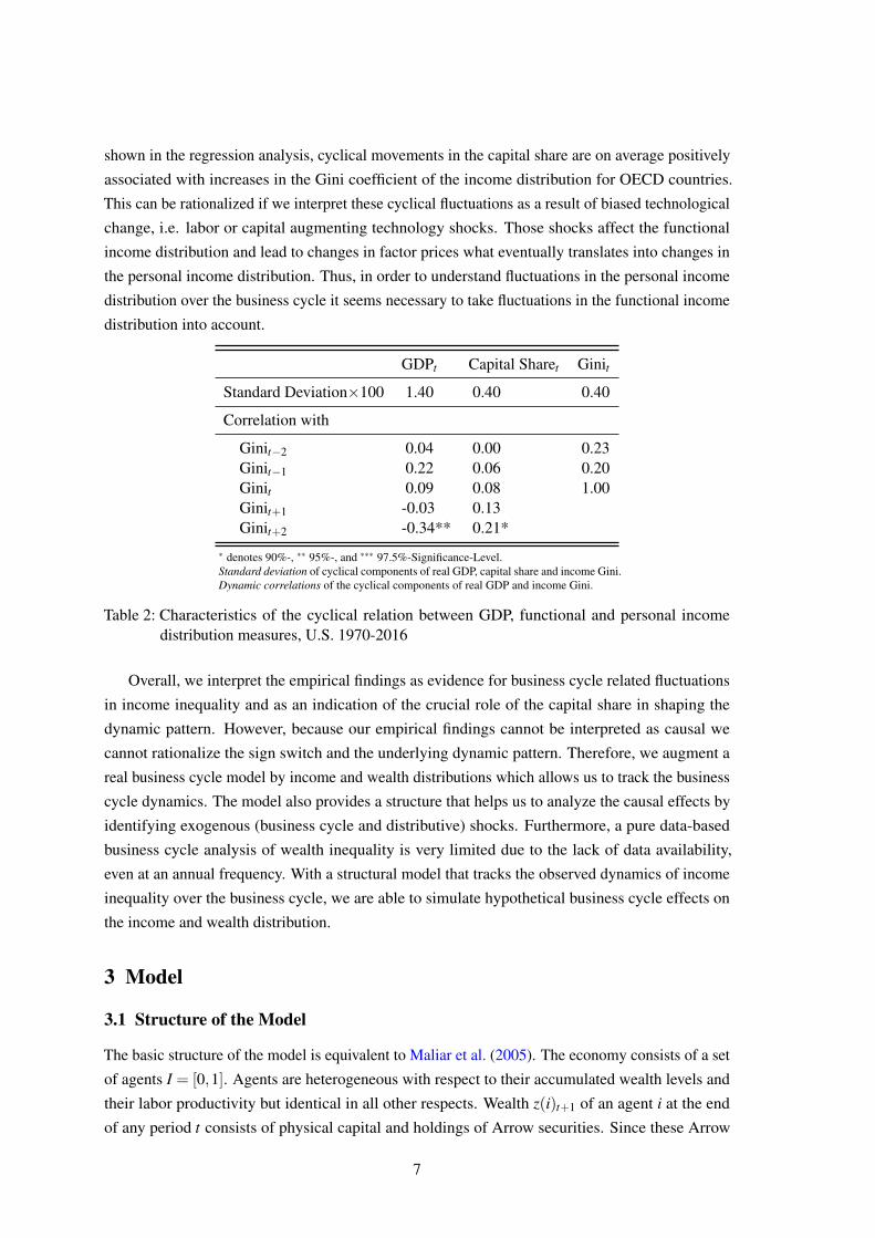
shown in the regression analysis, cyclical movements in the capital share are on average positively

associated with increases in the Gini coefficient of the income distribution for OECD countries.

This can be rationalized if we interpret these cyclical fluctuations as a result of biased technological

change, i.e. labor or capital augmenting technology shocks. Those shocks affect the functional

income distribution and lead to changes in factor prices what eventually translates into changes in

the personal income distribution. Thus, in order to understand fluctuations in the personal income

distribution over the business cycle it seems necessary to take fluctuations in the functional income

distribution into account.

GDPt Capital Sharet Ginit

Standard Deviation×100 1.40 0.40 0.40

Correlation with

Ginit−2 0.04 0.00 0.23Ginit−1 0.22 0.06 0.20Ginit 0.09 0.08 1.00Ginit+1 -0.03 0.13Ginit+2 -0.34** 0.21*

∗ denotes 90%-, ∗∗ 95%-, and ∗∗∗ 97.5%-Significance-Level.Standard deviation of cyclical components of real GDP, capital share and income Gini.Dynamic correlations of the cyclical components of real GDP and income Gini.

Table 2: Characteristics of the cyclical relation between GDP, functional and personal incomedistribution measures, U.S. 1970-2016

Overall, we interpret the empirical findings as evidence for business cycle related fluctuations

in income inequality and as an indication of the crucial role of the capital share in shaping the

dynamic pattern. However, because our empirical findings cannot be interpreted as causal we

cannot rationalize the sign switch and the underlying dynamic pattern. Therefore, we augment a

real business cycle model by income and wealth distributions which allows us to track the business

cycle dynamics. The model also provides a structure that helps us to analyze the causal effects by

identifying exogenous (business cycle and distributive) shocks. Furthermore, a pure data-based

business cycle analysis of wealth inequality is very limited due to the lack of data availability,

even at an annual frequency. With a structural model that tracks the observed dynamics of income

inequality over the business cycle, we are able to simulate hypothetical business cycle effects on

the income and wealth distribution.

3 Model

3.1 Structure of the Model

The basic structure of the model is equivalent to Maliar et al. (2005). The economy consists of a set

of agents I = [0,1]. Agents are heterogeneous with respect to their accumulated wealth levels and

their labor productivity but identical in all other respects. Wealth z(i)t+1 of an agent i at the end

of any period t consists of physical capital and holdings of Arrow securities. Since these Arrow

7

securities are in zero net supply,∫

I z(i)t+1di = kt+1 holds, where kt+1 denotes average physical

wealth. Labor productivity of agent i ∈ I is denoted by e(i).

The production side of the economy is essentially the same as in a canonical standard real

business cycle model with stochastic shocks to technology. However, in addition to the usual

technology shocks, distributive shocks — as in Lansing (2015) and Rıos-Rull and Santaeulalia-

Llopis (2010) — are included. The final output yt is produced by the following function:

yt = exp(θt)kαtt h1−αt

t , (1)

where firms use physical capital kt and labor ht . Here exp(θt) represents the level of productivity

with θt following an AR(1) process, i.e. θt+1 = ρθ θt + εθ ,t . The capital share αt can be used as

measure for the functional income distribution.8 In contrast to the canonical real business cycle

model it is assumed to be stochastic with

αt =aexp(ζt)

1+aexp(ζt)

, where ζt represents a distributive shock that follows the AR(1) process ζt+1 = ρζ ζt + εζ ,t and a is

a parameter that can be used to calibrate the functional income distribution.9

Each agent maximizes his expected lifetime utility, where preferences are assumed to be of the

GHH type, i.e. the period utility function of agent i is

u(i)t =

(c(i)t −B h(i)1+γ

t1+γ

)1−η

1−η, γ,η > 0,

where ct(i) denotes the individual real consumption, ht(i) individual labour supply, η , γ and B are

parameters measuring the intertemporal substitution elasticity, the inverse Frisch labor elasticity

and the relative preference for leisure.

As these preferences are of the Gorman form, there exists a representative consumer and

aggregate dynamics are independent of the wealth distribution. Define labor productivity of the

representative agent by e = (∫ 1

0 e(i)1+γ

γ di)γ

1+γ and let xt = ct −B h1+γ

t1+γ

. Aggregate dynamics are then

fully determined by the following set of equations (and a transversality condition which is not

8See Rıos-Rull and Santaeulalia-Llopis (2010).9For reasons of clarity in the presentation of the theoretical model we ignore possible spillover effects between both

types of productivity shocks, as they were emphasized by Rıos-Rull and Santaeulalia-Llopis (2010). However, in thequantitative assessment of the model, we incorporate a bi-variate shock process to take these effects into account.

8

displayed here):

x−η

t = βEt

[Rt+1x−η

t+1

](2a)

exp(θt)kαtt (eht)

1−αt = ct + kt+1− (1−δ )kt (2b)

ht =(wte

B

)1/γ

(2c)

xt = ct −Bh1+γ

t

1+ γ(2d)

Rt = 1−δ +αtexp(θt)kαt−1t (eht)

1−αt (2e)

wt = (1−αt)exp(θt)kαtt (eht)

−αt (2f)

θt+1 = ρθ θt + εθ ,t (2g)

ζt+1 = ρζ ζt + εζ ,t , (2h)

The intertemporal Euler equation (2a), the budget constraint (2b), the optimal labor supply (2c)

and the intratemporal utility (2d) determine the household behavior. The factor price equations for

capital (2e) and labor (2f) determine firm behavior. The model dynamics are initiated by TFP (2g)

and distributive shocks (2h).

While some initial values k0, θ0 as well as ζ0 are required to use these equations for the

computation of simulated time paths of aggregate variables, it is well known that the stochastic

properties of these aggregate variables do not depend on initial values. As will become clear below,

this is not the case for variables that describe the evolution of the cross sectional distribution of

these variables.

In order to describe the cross sectional distributions of some variables of interest, we now look

at the individual decision rules which are for all t the solution of the following problem:

max{c(i)t ,h(i)t ,k(i)t+1}∞

t=0

Et

∞

∑s=0

βs x(i)1−η

t+s

1−η(3)

s.t.

Rtk(i)t + e(i)wth(i)t +m(i)t(θt ,ζt) = c(i)t + k(i)t+1 +∫

Θ,Zpt(θ ,ζ )m(i)t+1(θ ,ζ )dθdζ

x(i)t = c(i)t −Bh(i)1+γ

t

1+ γ

θt+1 = ρθ θt + εθ ,t

ζt+1 = ρζ ζt + εζ ,t

Here m(i)t+1(θ ,ζ ) denotes agents i’s purchases of Arrow securities that pay out one unit in period

t+1 if θt+1 = θ and ζt+1 = ζ and p(i)t(θ ,ζ ) denotes the respective price of these Arrow securities.

The gross interest rate Rt and the real wage wt are quantities that depend on aggregate state

variables, i.e. Rt = R(kt ,θt ,ζt) and wt = w(kt ,θt ,ζt). Optimization is also subject to the initial

9

wealth endowment κ of agent i, which is given by:

κ(i) = R0k(i)0 +m(i)0(θ0,ζ0) (4)

Individual optimization (i.e. the Euler equation and the transversality condition) then implies (see

Maliar et al. (2005) for a proof) that for all t the following equation holds:

c(i)t − e(i)wth(i)t + k(i)t+1

+∫

Θ,Zpt(θ ,ζ )m(i)t+1(θ ,ζ )dθdζ = Rtk(i)t +m(i)t(θt ,ζt)

= Et

[∞

∑s=0

βs x(i)−η

t+s

x(i)−η

t(c(i)t+s− e(i)h(i)t+swt+s)

] (5)

With z(i)t+1 = k(i)t+1 +∫

Θ,Z pt(θ ,ζ )m(i)t+1(θ ,ζ )dθdζ denoting the wealth level of agent i at

the end of period t, equation (5) can be rewritten as:

z(i)t+1 = wt − c(i)t +Et

[∞

∑s=0

βs x(i)−η

t+s

x(i)−η

t(c(i)t+s− e(i)h(i)t+swt+s)

]

= Et

[∞

∑s=1

βs x(i)−η

t+s

x(i)−η

t(c(i)t+s− e(i)h(i)t+swt+s)

]

Using the first order condition for optimal labor supply and the fact that the Gorman form of

preferences implies that x(i)t = µ(i)xt for all t, this equation can be rearranged to get:

z(i)t+1 =

(µ(i)−

(e(i)

e

) 1+γ

γ

)Et

∞

∑s=1

βs x1−η

t+s

x−η

t+

(e(i)

e

) 1+γ

γ

zt+1

Finally, let φ(i) = (e(i)/e)1+γ

γ (notice, that∫ 1

0 φ(i)di = 1) and define Ut = Et ∑∞s=0 β sx1−η

t+s , where

Ut follows the recursive equation:10

EtUt+1 =1β(Ut − x1−η

t ) (6)

We then get that the wealth share a(i)t = z(i)t/kt of agent i evolves over time according to:

a(i)t+1 = (µ(i)−φ(i))xη

t Ut − xt

kt+1+φ(i) (7)

3.2 Distributional Dynamics

Besides the initial values for the state variables (i.e. k0, θ0 and ζ0) the initial cross sectional

distributions of wealth endowments as well as productivities have to be specified in order to

describe the distributional dynamics implied by the model.

10Notice, that Ut is proportional (up to the constant 1/(1−η)) to expected utility of the representative agent and that Utboils down to the constant 1/(1−β ) when η = 1.

10

In what follows, the distribution of initial wealth shares a(i) = κ(i)/(R0k0) as well as the

distribution of transformed productivities φ(i) are regarded as exogenous objects. With this,

equation (5) evaluated at t = 0 implies that the share µ(i) = x(i)t/xt of agent i is given by:

µ(i) = [a(i)−φ(i)]R0k0

xη

0 U0+φ(i) (8)

Equation (8) determines the time invariant share µ(i) in dependence on the initial conditions

of the model. Since x(i)t has to be greater than zero for all i, this equation in fact formulates a

restriction over these initial conditions that has to be met:

Assumption 1 The initial distributions a(i) and φ(i) are such that for all i ∈ I:

[a(i)−φ(i)]R0k0

xη

0 U0+φ(i)> 0 (A.1)

In what follows we will generally assume that (A.1) is satisfied. Using (8), equation (7) describing

the evolution of the wealth distribution now becomes

a(i)t+1 = [a(i)−φ(i)]p0qt , t = 0,1,2, ... (9)

where

pt =Rtkt

xη

t Ut, qt =

xη

t Ut − xt

kt+1.

where pt can be interpreted as capital value weighted in utility terms. The initial value of end of

period wealth holdings a(i)1 is completely determined by the exogenous initial cross sectional

distributions of wealth holdings a(i) and labor productivities φ(i) as well as the initial values of the

aggregate state variables (which pin down the values of R0,k0,x0,U0 and k1). Thus, the dynamic

properties of the wealth distribution also depend on initial values of aggregate state variables.

Equation (9) describes the dynamic evolution of the wealth distribution and given this it is

possible to describe all other relevant cross sectional distributions. First, note that the transformed

productivities φ(i) = (e(i)/e)1+γ

γ , are by construction equivalent to the ratio of individual efficiency

hours worked to average efficiency hours and thus equivalent to the — therefore time invariant —

ratio ω(i) = wt e(i)h(i)twt eht

of individual labor income to average labor income.11 The cross sectional

distribution of factor incomes can be computed from the model if it is assumed that there is no

trade of contingent claims in equilibrium.12 While this will leave the individual lifetime budget

constraints and therefore the allocation unchanged, it implies via (4) that a(i) = a(i)0 and that the

share y(i)t of agent i in total factor income in period t is given by:

y(i)t = αta(i)t +(1−αt)φ(i) (10)

11Because h(i)t = (wte(i)/B)1/γ and ht = (wte/B)1/γ , we have (e(i)h(i)t)/(eht) = (e(i)/e)(1+γ)/γ = φ(i).12See on this Maliar et al. (2005), who make the point that the lifetime budget constraints of the agents remain unchanged

if there is no trade of contingent claims. However, if one wants to model an economy where some agents are initiallyindebted, this requires k(i)0 < 0 such that k(i)t cannot be interpreted as an agent’s holding of physical capital. In thiscase k(i)t represents individual net worth which aggregates to the aggregate capital stock kt as the sum of all debt hasto be zero.

11

Under the harmless assumption that a(i) and φ(i) are both continuous on I, it is always possible

to compute from equations (9) and (10) at least variances and covariances in a straightforward way

in order to describe the dynamics of the cross sectional distributions of wealth and income. So for

instance, the coefficient of variation σa,t of a(i)t evolves according to:

σa,t+1 =√

(p0qt)2σ2a +(1− p0qt)2σ2

φ+2p0qt(1− p0qt)σ2

a,φ , (11)

where σ2a and σ2

φdenote the cross sectional variances of a and φ , respectively and σ2

a,φ denotes the

cross sectional covariance between a and φ .

Of course, a more convenient way to characterize the distributional implications of the model

would be to consider usual inequality measures like Gini coefficients. Below we will present

equations that describe the approximated (i.e. linearized) dynamics of Gini coefficients.13 First,

however, we will look at a special case that allows for a straightforward computation of Gini

coefficients from the cross sectional distributions generated by the model. This case arises when

a(i) and φ(i) satisfy some preconditions that are summarized below:

Assumption 2 The initial distributions a(i) and φ(i) are such that for all i ∈ I = [0,1]:

(i) φ(i) is integrable and monotone increasing,

(ii) a(i) is integrable and monotone increasing,

(iii) a(i)−φ(i) is integrable and monotone increasing.

Conditions (i) and (ii) imply that the Gini coefficients of the initial wealth and productivity

distributions can be constructed simply by integration of φ(i) and a(i). So, for instance, the Gini

coefficient of the initial wealth distribution is given by Ga = 1−2∫ i

0∫ j

0 a(i)didj.14 As equation (9)

reveals, condition (iii) then ensures that a(i)t+1 is for all t ≥ 0 integrable and monotone increasing

on I such that the Gini coefficient Ga,t+1 of the wealth distribution at the end of period t can be

constructed also simply by integration of a(i)t+1. Finally this implies that y(i)t is also integrable

and monotone increasing such that the Gini coefficient of the income distribution Gy,t results by

integrating y(i)t . From (9) and (10) we therefore get:

Ga,t+1 = p0qtGa+(1− p0qt)Gφ , (12a)

Gy,t = αt p0qt−1Ga+(1−αt p0qt−1)Gφ (12b)

with pt and qt as defined in (9) and with Ga and Gφ denoting the exogenously given Gini coefficients

of the endowment distributions. Notice that p0 and the dynamics of qt are completely determined

by the model parameters and the initial values of the aggregate state variables. Thus, together with

Ga and Gφ this then determines the dynamics of wealth and income inequality.

13In Appendix B we show how to derive a linearized representation of the coefficient of variation. In Appendix C wepresent a linearized version of a generalized entropy index. However, note that the cyclical variations of all theseinequality measures are related through qt and are proportional to each other.

14Note that the Lorenz curve of the initial wealth distribution La( j) is given by La( j) =∫ j

0 a(i)di.

12

A special feature of the distributional dynamics described by equations (11) as well as (12a)

and (12b) is that the cross sectional dynamics still depend on the initial value p0. However, we will

get rid of this initial value when we analyze the linearized dynamics of the inequality measures in

the neighborhood of the steady state of the model. The resulting linearized counterparts of (12a)

and (12b) are given by:

Ga,t+1 = qt

(1−

Gφ

Ga

), (13a)

Gy,t = [qt−1 + αt ]

(1−

Gφ

Gy

), (13b)

where – as usual – the hat indicates that a variable represents a relative deviation from the respective

steady state.15 In equations (13a) and (13b) Gφ is the exogenous inequality measure for labor

income and all other variables without a time index represent respective steady state values.The

steady state values of inequality measures for wealth and income itself are related through the

following equation:

Gy = αGa +(1−α)Gφ (14)

To summarize, the complete set of linearized equations describing aggregate as well as dis-

tributional dynamics is given by the linearized equations (2a) – (2h) from above as well as the

linearizations of (6) and the equation that defines qt :

EtUt+1 =1β

Ut +(1−η)1−β

βEt xt+1 (15a)

qt =η +β −1

βxt +

1β

Ut − kt+1 (15b)

Thus, augmenting an otherwise conventional stochastic macroeconomic model with the just

derived equations enables us to describe and simulate the distributional implications of exogenous

shocks in that model. Moreover, equation (13a) and (13b), allow to derive some first conclusions

regarding the business cycle properties of wealth and income inequality.

Concerning this, let us first look at the volatility of income and wealth inequality. Equations

(13a) and (13b) reveal that this volatility depends on the one hand on the volatility of the aggregate

variables qt and αt and on the other hand on the cross sectional distribution of the stochastic steady

state as determined by Ga and Gφ . There are two special cases where there is no volatility in

inequality at all such that the wealth and income distributions remain unchanged over time. The

first one is the case where qt as well as αt are constant over time. While αt is constant whenever

there are no distributional shocks, qt stays constant only for certain parameterizations (η = 1) of the

model (we will come back to this in the next section). The second case is the one where a(i) = φ(i)

for all i ∈ I (cf. equations (9) and (10)). In this case we have Ga = Gφ , such that wealth and income

inequality stay constant over time. Besides this, (13a) and (13b) allow for the conclusion that

the volatility of wealth and income inequality will be larger, the larger the differences between

15We should note that the equations for Gini coefficients (13a) and (13b) are in fact exact representations of the truedynamics as long as the conditions of Assumption 2 are satisfied.

13

wealth, labor income and total income distributions are. Another relevant business cycle feature

is the cyclical behavior of wealth and income inequality. Regarding this, assume first that there

are no distributive shocks (i.e. αt = 0) and that the model is calibrated in a more or less plausible

way such that Ga > Gφ . In this case wealth inequality moves in the same direction as qt , i.e.

wealth inequality behaves procyclical whenever qt does so (and we will show later that a plausible

calibration of the model implies that qt is in fact proyclical).

4 Quantitative Analysis

4.1 Shocks and Inequality

In order to assess the consequences of exogenous technology shocks for wealth inequality, it

is useful to neglect any distributive shocks and to look at the dynamics of wealth inequality in

a deterministic model first. Chatterjee (1994) and Caselli and Ventura (2000) performed such

analyses and the latter paper shows that with η = 1 and Cobb–Douglas technology the transition

towards the deterministic steady state from below (above) goes along with declining (rising) wealth

inequality. While this suggests that a positive technology shock in an equivalent stochastic model

should go along with a decline in wealth inequality, we will see that this is not necessarily true as

the serial correlation of the technology shocks also matters for the response of wealth inequality.

To see this, look at the ratios xtkt+1

ktxt−1

that govern the dynamics of wealth inequality in the case

the elasticity of intertemporal substitution is η = 1 (cf. eqn. (7)).16 Assume that in period t the

economy is hit by a purely transitory and positive technology shock. Starting from xt−1 = x∗ and

kt = k∗, both xt as well as kt+1 will increase, with the increase in xt being smaller than the increase

in kt+1. As a consequence, xt/kt+1 < x∗/k∗ and wealth inequality will decline. If, however, the

productivity shocks display a high enough degree of serial correlation, the increase in xt might

well be larger than the increase in kt+1, such that wealth inequality rises in response to a positive

technology shock. This results because an anticipated long lasting future increase in TFP requires

not that much investment.

TFP shocksFigure 3 shows typical impulse responses of wealth inequality to a positive technology shock for

different values of some of the model’s parameters.17 The upper panel shows impulse responses for

the case of serially uncorrelated shocks, the lower panel shows the responses for serially correlated

shocks. As can be seen, whether or not wealth inequality increases in response to a positive

technology shock — and thus behaves procyclical — depends on the intertemporal elasticity of

substitution 1/η and the persistence of productivity shocks ρθ . In case shocks are not persistent,

a negative response results for low enough values of η < 1 or, conversely, a positive response

now requires a large enough value of η > 1. For plausible values of η ≈ 2 and ρθ ≈ 0.95 wealth

inequality rises on impact and then converges back to its steady state level. From the business cycle

16η = 1 implies xη

t Ut−xtkt+1

= β

1−β

xtkt+1

.17The underlying model is calibrated – with respect to quarterly data – with β = 0.988, δ = 0.025, α = 0.38. We set

Gy to 0.43 and Ga is set to 0.8. We plot the impulse responses only for wealth inequality, because the reactions ofthe wealth and income distribution are identical in case of TFP shocks.

14

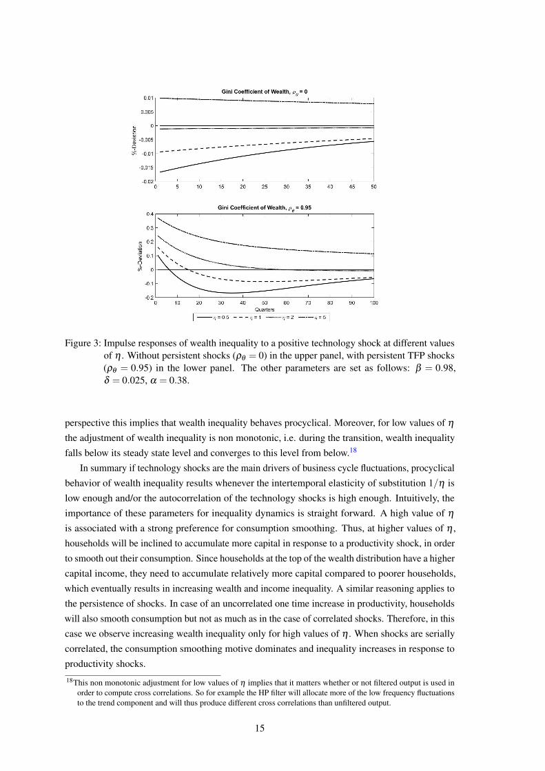
Figure 3: Impulse responses of wealth inequality to a positive technology shock at different valuesof η . Without persistent shocks (ρθ = 0) in the upper panel, with persistent TFP shocks(ρθ = 0.95) in the lower panel. The other parameters are set as follows: β = 0.98,δ = 0.025, α = 0.38.

perspective this implies that wealth inequality behaves procyclical. Moreover, for low values of η

the adjustment of wealth inequality is non monotonic, i.e. during the transition, wealth inequality

falls below its steady state level and converges to this level from below.18

In summary if technology shocks are the main drivers of business cycle fluctuations, procyclical

behavior of wealth inequality results whenever the intertemporal elasticity of substitution 1/η is

low enough and/or the autocorrelation of the technology shocks is high enough. Intuitively, the

importance of these parameters for inequality dynamics is straight forward. A high value of η

is associated with a strong preference for consumption smoothing. Thus, at higher values of η ,

households will be inclined to accumulate more capital in response to a productivity shock, in order

to smooth out their consumption. Since households at the top of the wealth distribution have a higher

capital income, they need to accumulate relatively more capital compared to poorer households,

which eventually results in increasing wealth and income inequality. A similar reasoning applies to

the persistence of shocks. In case of an uncorrelated one time increase in productivity, households

will also smooth consumption but not as much as in the case of correlated shocks. Therefore, in this

case we observe increasing wealth inequality only for high values of η . When shocks are serially

correlated, the consumption smoothing motive dominates and inequality increases in response to

productivity shocks.

18This non monotonic adjustment for low values of η implies that it matters whether or not filtered output is used inorder to compute cross correlations. So for example the HP filter will allocate more of the low frequency fluctuationsto the trend component and will thus produce different cross correlations than unfiltered output.

15

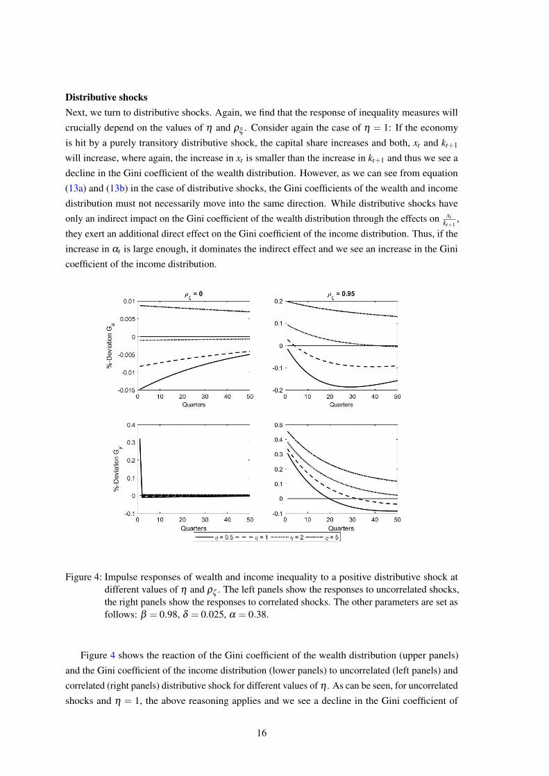
Distributive shocksNext, we turn to distributive shocks. Again, we find that the response of inequality measures will

crucially depend on the values of η and ρξ . Consider again the case of η = 1: If the economy

is hit by a purely transitory distributive shock, the capital share increases and both, xt and kt+1

will increase, where again, the increase in xt is smaller than the increase in kt+1 and thus we see a

decline in the Gini coefficient of the wealth distribution. However, as we can see from equation

(13a) and (13b) in the case of distributive shocks, the Gini coefficients of the wealth and income

distribution must not necessarily move into the same direction. While distributive shocks have

only an indirect impact on the Gini coefficient of the wealth distribution through the effects on xtkt+1

,

they exert an additional direct effect on the Gini coefficient of the income distribution. Thus, if the

increase in αt is large enough, it dominates the indirect effect and we see an increase in the Gini

coefficient of the income distribution.

Figure 4: Impulse responses of wealth and income inequality to a positive distributive shock atdifferent values of η and ρζ . The left panels show the responses to uncorrelated shocks,the right panels show the responses to correlated shocks. The other parameters are set asfollows: β = 0.98, δ = 0.025, α = 0.38.

Figure 4 shows the reaction of the Gini coefficient of the wealth distribution (upper panels)

and the Gini coefficient of the income distribution (lower panels) to uncorrelated (left panels) and

correlated (right panels) distributive shock for different values of η . As can be seen, for uncorrelated

shocks and η = 1, the above reasoning applies and we see a decline in the Gini coefficient of

16

the wealth distribution accompanied by a rise in the Gini coefficient of the income distribution.

This pattern changes when either η increases or the correlation of distributive shocks is taken into

account. For η > 2 both Gini coefficients show procyclical behavior in the case of uncorrelated

shocks.

4.2 Matching to U.S. data

Next, in order to find an empirically plausible specification, we use Bayesian methods to match

a subset of the model parameters to U.S. data. In a second step, we then compare the simulated

Gini path with the historical data series. To this end, we focus mostly on the stochastic process for

productivity θt and the process that describes distributive shocks ζt . Moreover, we are especially

interested in the parameter that is particularly relevant for the reaction of inequality measures,

i.e. the inverse of η . In the specification for the estimation, we take the results of Rıos-Rull and

Santaeulalia-Llopis (2010), as a starting point and specify a bivariate process of productivity as

follows:19 [θt

ζt

]=

[ρθ ρθ ,ζ

ρζ ,θ ρζ

][θt−1

ζt−1

]+

[εθ ,t

εζ ,t

](16)

where ρθ ,ζ and ρζ ,θ denote the off-diagonal elements of the coefficient matrix. In addition, in

order to make the estimation of the intertemporal elasticity of substitution more robust, we add

observational errors to consumption.

The data series for the estimation for the United States were retrieved from Bureau of Economic

Analysis (BEA) and the Bureau of Labor Statistics (BLS). As observables, we use real per capita

GDP, the capital share and real private consumption per capita. The data are available for the

period 1948Q1:2017Q4. All series are seasonally adjusted, and we apply a one-sided HP filter with

λ = 1600 to isolate the cyclical components of the series.

4.3 Calibration and Priors

As it is common in the literature, we calibrate a set of parameters to match general properties of

the US economy. In particular, we set β to 0.988, this gives an annual steady state interest rate of

approximately 4.8%. The depreciation rate δ is set to be 0.025, which gives an annual depreciation

of 10%, as it is common with quarterly data. Steady state aggregate labor input is calibrated to

match the average working time in the United States, we set B to 5.06 and γ = 0.5, this results in

average hours worked of 0.23 which translates into 38.6 average working time per week (fulltime

equivalent). Regarding the distributional implications of the model, parameters to be determined

are Gφ , Ga and Gy. Here calibration targets Ga and Gφ for steady state wealth and labor income

inequality together with α deliver via (14) a unique value for Gy. However, as Ga, Gφ and Gy

are tied to each other via (14) not any desired combination of these inequality measures can be

reproduced by the model. Whenever we start from the empirical fact that the wealth distribution is

19This choice reflects the lack of a clear cut understanding of the relationship between both shock processes.We alsoexamine the model dynamics for the case where both shocks are i.i.d. AR(1) processes, as they are commonlyemployed in the literature. The main conclusions presented below remain unaffected by this choice and thecorresponding results are available upon request.

17

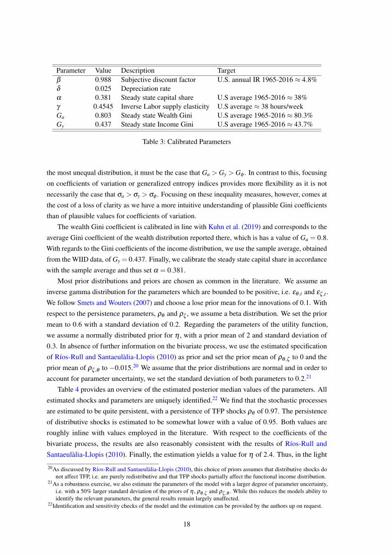
Parameter Value Description Targetβ 0.988 Subjective discount factor U.S. annual IR 1965-2016 ≈ 4.8%δ 0.025 Depreciation rateα 0.381 Steady state capital share U.S average 1965-2016 ≈ 38%γ 0.4545 Inverse Labor supply elasticity U.S average ≈ 38 hours/weekGa 0.803 Steady state Wealth Gini U.S average 1965-2016 ≈ 80.3%Gy 0.437 Steady state Income Gini U.S average 1965-2016 ≈ 43.7%

Table 3: Calibrated Parameters

the most unequal distribution, it must be the case that Ga > Gy > Gφ . In contrast to this, focusing

on coefficients of variation or generalized entropy indices provides more flexibility as it is not

necessarily the case that σa > σy > σφ . Focusing on these inequality measures, however, comes at

the cost of a loss of clarity as we have a more intuitive understanding of plausible Gini coefficients

than of plausible values for coefficients of variation.

The wealth Gini coefficient is calibrated in line with Kuhn et al. (2019) and corresponds to the

average Gini coefficient of the wealth distribution reported there, which is has a value of Ga = 0.8.

With regards to the Gini coefficients of the income distribution, we use the sample average, obtained

from the WIID data, of Gy = 0.437. Finally, we calibrate the steady state capital share in accordance

with the sample average and thus set α = 0.381.

Most prior distributions and priors are chosen as common in the literature. We assume an

inverse gamma distribution for the parameters which are bounded to be positive, i.e. εθ ,t and εζ ,t .

We follow Smets and Wouters (2007) and choose a lose prior mean for the innovations of 0.1. With

respect to the persistence parameters, ρθ and ρζ , we assume a beta distribution. We set the prior

mean to 0.6 with a standard deviation of 0.2. Regarding the parameters of the utility function,

we assume a normally distributed prior for η , with a prior mean of 2 and standard deviation of

0.3. In absence of further information on the bivariate process, we use the estimated specification

of Rıos-Rull and Santaeulalia-Llopis (2010) as prior and set the prior mean of ρθ ,ζ to 0 and the

prior mean of ρζ ,θ to −0.015.20 We assume that the prior distributions are normal and in order to

account for parameter uncertainty, we set the standard deviation of both parameters to 0.2.21

Table 4 provides an overview of the estimated posterior median values of the parameters. All

estimated shocks and parameters are uniquely identified.22 We find that the stochastic processes

are estimated to be quite persistent, with a persistence of TFP shocks ρθ of 0.97. The persistence

of distributive shocks is estimated to be somewhat lower with a value of 0.95. Both values are

roughly inline with values employed in the literature. With respect to the coefficients of the

bivariate process, the results are also reasonably consistent with the results of Rıos-Rull and

Santaeulalia-Llopis (2010). Finally, the estimation yields a value for η of 2.4. Thus, in the light

20As discussed by Rıos-Rull and Santaeulalia-Llopis (2010), this choice of priors assumes that distributive shocks donot affect TFP, i.e. are purely redistributive and that TFP shocks partially affect the functional income distribution.

21As a robustness exercise, we also estimate the parameters of the model with a larger degree of parameter uncertainty,i.e. with a 50% larger standard deviation of the priors of η , ρθ ,ζ and ρζ ,θ . While this reduces the models ability toidentify the relevant parameters, the general results remain largely unaffected.

22Identification and sensitivity checks of the model and the estimation can be provided by the authors up on request.

18

of the preceding discussion, since shocks are found to be persistent and since the intertemporale

elasticity of substitution is sufficiently small, we expect inequality measures to react procyclical to

TFP shocks on impact.

Prior Posteriorparameter value type mean std mode mean

Volatility

TFP σθ ,t IG 0.1 2 0.01 0.01Distr. σζ ,t IG 0.1 2 0.02 0.02

Persistence

TFP ρθ B 0.6 0.2 0.97 0.94Distr. ρζ B 0.6 0.2 0.95 0.95

Cross-Coefficients

TFP-Distr. ρθ ,ζ N 0.0 0.1 0.18 0.16Distr.-TFP ρζ ,θ N -0.01 0.1 -0.10 -0.11

Utility function

SE Intertemporal η N 2 0.3 2.38 2.41

Table 4: Prior and Posterior distribution of the estimated parameters. The posterior distribution isobtained using the Meteropolis-Hastings algorithm with 2 MCMC chains to generate asample of 500.000 draws each.

4.4 Shock contribution and historical comparison

We analyze the estimated behavior of macroeconomic variables and inequality measures to shocks

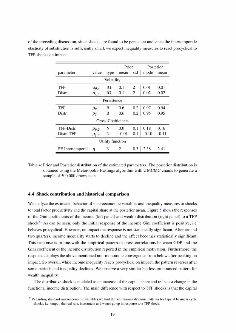
to total factor productivity and the capital share at the posterior mean. Figure 5 shows the responses

of the Gini coefficients of the income (left panel) and wealth distribution (right panel) to a TFP

shock23 As can be seen, only the initial response of the income Gini coefficient is positive, i.e.

behaves procyclical. However, on impact the response is not statistically significant. After around

two quarters, income inequality starts to decline and the effect becomes statistically significant.

This response is in line with the empirical pattern of cross-correlations between GDP and the

Gini coefficient of the income distribution reported in the empirical motivation. Furthermore, the

response displays the above mentioned non-monotonic convergence from below after peaking on

impact. So overall, while income inequality reacts procyclical on impact, the pattern reverses after

some periods and inequality declines. We observe a very similar but less pronounced pattern for

wealth inequality.

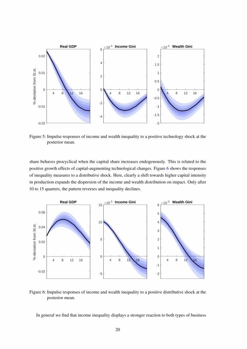
The distributive shock is modeled as an increase of the capital share and reflects a change in the

functional income distribution. The main difference with respect to TFP shocks is that the capital

23Regarding standard macroeconomic variables we find the well known dynamic patterns for typical business cycleshocks, i.e. output, the real rate, investment and wages go up in response to a TFP shock.

19

Real GDP

4 8 12 16

-0.02

-0.01

0

0.01

0.02

%-d

evia

tion

from

St.s

t.

Income Gini

4 8 12 16

-4

-2

0

2

4

610-3 Wealth Gini

4 8 12 16

-2

-1.5

-1

-0.5

0

0.5

1

1.5

2

10-3

Figure 5: Impulse responses of income and wealth inequality to a positive technology shock at theposterior mean.

share behaves procyclical when the capital share increases endogenously. This is related to the

positive growth effects of capital-augmenting technological changes. Figure 6 shows the responses

of inequality measures to a distributive shock. Here, clearly a shift towards higher capital intensity

in production expands the dispersion of the income and wealth distribution on impact. Only after

10 to 15 quarters, the pattern reverses and inequality declines.

Real GDP

4 8 12 16

-0.02

0

0.02

0.04

0.06

%-d

evia

tion

from

St.s

t.

Income Gini

4 8 12 16

-5

0

5

10

1510-3 Wealth Gini

4 8 12 16

-2

-1

0

1

2

3

4

5

610-3

Figure 6: Impulse responses of income and wealth inequality to a positive distributive shock at theposterior mean.

In general we find that income inequality displays a stronger reaction to both types of business

20

cycle shocks compared to the reaction of wealth inequality. This suggests that wealth inequality is

less susceptible to cyclical fluctuations.24 This finding seems intuitive, while changes in wealth

inequality are bound to changes in the individual capital stock, which requires an adjustment

period, changes in income inequality can materialize directly in response to changes in factor prices.

The more pronounced reaction of the Gini coefficient of the income distribution in response to

distributive shocks relative to standard TFP shocks can be explained by the direct effect which

the distributive shock exerts on the income composition. Intuitively, the redistribution of income

towards capital is clearly in favor of wealthier households. Given the assumed functional forms, the

distributive shock induces a rise in the real interest rate and an expansion of output. This leads to

an increase in investment which translates into a higher capital stock, what eventually leads to an

increase in wages. This pattern conforms with the notion of productivity shocks that diffuse slowly

into production and primarily benefit capital income, while labor income increases only with a delay

after a couple of periods. In contrast, a standard TFP shock increases overall productivity, which

induces a broadly proportional increase in labor and capital income, resulting in less dispersion in

income.

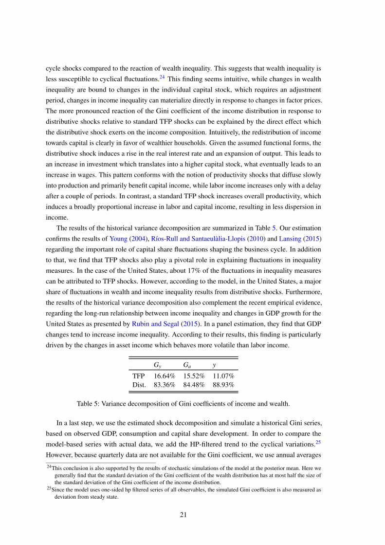
The results of the historical variance decomposition are summarized in Table 5. Our estimation

confirms the results of Young (2004), Rıos-Rull and Santaeulalia-Llopis (2010) and Lansing (2015)

regarding the important role of capital share fluctuations shaping the business cycle. In addition

to that, we find that TFP shocks also play a pivotal role in explaining fluctuations in inequality

measures. In the case of the United States, about 17% of the fluctuations in inequality measures

can be attributed to TFP shocks. However, according to the model, in the United States, a major

share of fluctuations in wealth and income inequality results from distributive shocks. Furthermore,

the results of the historical variance decomposition also complement the recent empirical evidence,

regarding the long-run relationship between income inequality and changes in GDP growth for the

United States as presented by Rubin and Segal (2015). In a panel estimation, they find that GDP

changes tend to increase income inequality. According to their results, this finding is particularly

driven by the changes in asset income which behaves more volatile than labor income.

Gy Ga y

TFP 16.64% 15.52% 11.07%Dist. 83.36% 84.48% 88.93%

Table 5: Variance decomposition of Gini coefficients of income and wealth.

In a last step, we use the estimated shock decomposition and simulate a historical Gini series,

based on observed GDP, consumption and capital share development. In order to compare the

model-based series with actual data, we add the HP-filtered trend to the cyclical variations.25

However, because quarterly data are not available for the Gini coefficient, we use annual averages

24This conclusion is also supported by the results of stochastic simulations of the model at the posterior mean. Here wegenerally find that the standard deviation of the Gini coefficient of the wealth distribution has at most half the size ofthe standard deviation of the Gini coefficient of the income distribution.

25Since the model uses one-sided hp filtered series of all observables, the simulated Gini coefficient is also measured asdeviation from steady state.

21

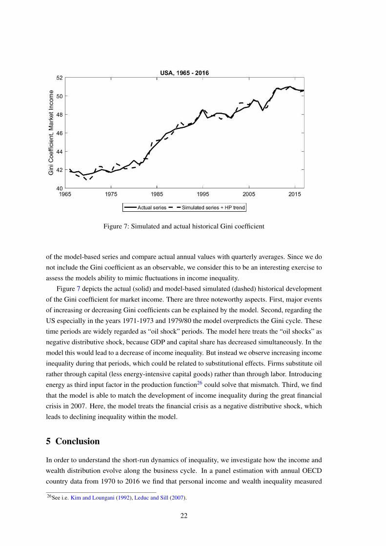
Figure 7: Simulated and actual historical Gini coefficient

of the model-based series and compare actual annual values with quarterly averages. Since we do

not include the Gini coefficient as an observable, we consider this to be an interesting exercise to

assess the models ability to mimic fluctuations in income inequality.

Figure 7 depicts the actual (solid) and model-based simulated (dashed) historical development

of the Gini coefficient for market income. There are three noteworthy aspects. First, major events

of increasing or decreasing Gini coefficients can be explained by the model. Second, regarding the

US especially in the years 1971-1973 and 1979/80 the model overpredicts the Gini cycle. These

time periods are widely regarded as “oil shock” periods. The model here treats the “oil shocks” as

negative distributive shock, because GDP and capital share has decreased simultaneously. In the

model this would lead to a decrease of income inequality. But instead we observe increasing income

inequality during that periods, which could be related to substitutional effects. Firms substitute oil

rather through capital (less energy-intensive capital goods) rather than through labor. Introducing

energy as third input factor in the production function26 could solve that mismatch. Third, we find

that the model is able to match the development of income inequality during the great financial

crisis in 2007. Here, the model treats the financial crisis as a negative distributive shock, which

leads to declining inequality within the model.

5 Conclusion

In order to understand the short-run dynamics of inequality, we investigate how the income and

wealth distribution evolve along the business cycle. In a panel estimation with annual OECD

country data from 1970 to 2016 we find that personal income and wealth inequality measured

26See i.e. Kim and Loungani (1992), Leduc and Sill (2007).

22

by the Gini coefficient are countercyclical and statistically significant on average. However, by

calculating country-specific cyclical correlations of inequality we detect a substantial cross-country

heterogeneity: More than half of all OECD countries display a countercyclical relationship between

output fluctuations and inequality. Yet, roughly one third of the countries, among others the United

States, show an acyclical or even procyclical pattern. In a detailed analysis of the cyclical properties

of the income Gini coefficient, we find that in the United States, income inequality is less volatile

than output, with a relative standard deviation of about one third.

To understand the driving forces of the income and wealth distribution over the business cycle

in more detail, we incorporate distributive shocks in a standard business cycle model, where agents

are ex-ante heterogeneous with respect to wealth and ability. We show that this framework allows to

derive linearized approximations standard inequality measures such as Gini coefficients. Applying

the model to our research question, we show that the cyclicality of these inequality measures

depends crucially on the parameters of the model and in particular on the intertemporal elasticity of

substitution. Thus, the behaviour of inequality is eventually an empirical question about the size of

these two paremters and the relative contribution of TFP as well as distributive shocks.

We match our model to quarterly data for the United States by estimating the shock processes

and relevant parameters of the model using Bayesian methods. We find that the intertemporal

elasticity of substitution is close to two and that the shock processes display a high degree of

persistence. Therefore, both, TFP and distributive shocks generate a procyclical reaction of

the income and wealth distribution on impact. However, in response to TFP shocks it declines

afterwards, which renders the effect countercyclical in later periods. In case of the distributive shock

the dynamics of the income and wealth distribution stays procyclical. This finding matches the

empirical cross-correlation pattern between GDP and the Gini coefficient of the income distribution

observed in the United States. Furthermore, we find that income inequality reacts more pronounced

to business cycle shocks compared to wealth inequality. According to the results of stochastic

simulations, the model predicts that wealth inequality is about half as volatile along the business

cycle as income inequality.

Finally, we analyze the relative shock contribution according to our posterior specification.

Here, we find that the model assigns the major share of fluctuations in inequality measures, roughly

85% to distributive shocks. Thus, our estimation confirms the important role of fluctuations in

factor shares, e.g. due to capital-augmenting technological change, in shaping the business cycle

and furthermore highlights its importance for short run inequality dynamics.

23

References

Ahn, SeHyoun, Greg Kaplan, Benjamin Moll, Thomas Winberry, and Christian Wolf, “When

Inequality Matters for Macro and Macro Matters for Inequality,” in “NBER Macroeconomics

Annual 2017, volume 32” NBER Chapters, National Bureau of Economic Research, Inc, 2017,

pp. 1–75.

Aiyagari, Rao S., “Uninsured Idiosyncratic Risk and Aggregate Saving,” The Quarterly Journal of

Economics, 1994, 109 (3), 659 – 684.

Alvaredo, Facundo, Lucas Chancel, Thomas Piketty, Emmanuel Saez, and Gabriel Zucman,

“Global Inequality Dynamics: New Findings from WID.world,” American Economic Review,

May 2017, 107 (5), 404–09.

Atkinson, A. B., “Factor shares: the principal problem of political economy?,” Oxford Review of

Economic Policy, 2009, 25 (1), 3 – 16.

Barro, Robert J, “Inequality and Growth in a Panel of Countries,” Journal of Economic Growth,

2000, 5 (1), 5–32.

Bayer, Christian and Ralph Luetticke, “Solving heterogeneous agent models in discrete time

with many idiosyncratic states by perturbation methods,” CEPR Discussion Papers 13071,

C.E.P.R. Discussion Papers July 2018.

and , “Shocks, Frictions, and Inequality in US Business Cycles,” Technical Report 2019.

Cantore, Cristiano, Filippo Ferroni, and Miguel A. Leon-Ledesma, “The Missing Link: Mon-

etary policy and the labor share,” Discussion Papers 1829, Centre for Macroeconomics (CFM)

November 2018.

Caselli, Francesco and Jaume Ventura, “A Representative Consumer Theory of Distribution,”

American Economic Review, 2000, 90 (4), 909 – 926.

Challe, Edouard, Julien Matheron, Xavier Ragot, and Juan F. Rubio-Ramirez, “Precautionary

saving and aggregate demand,” Quantitative Economics, 2017, 8 (2), 435–478.

Chatterjee, Satyajit, “Transitional dynamics and the distribution of wealth in a neoclassical growth

model,” Journal of Public Economics, 1994, 54 (1), 97 – 119.

Debortoli, Davide and Jordi Galı, “Monetary policy with heterogeneous agents: Insights from

TANK models,” Economics Working Papers 1686, Department of Economics and Business,

Universitat Pompeu Fabra September 2017.

Dimelis, Sophia and Alexandra Livada, “Inequality and business cycles in the U.S. and European

Union countries,” International Advances in Economic Research, Aug 1999, 5 (3), 321–338.

Feenstra, Robert C., Robert Inklaar, and Marcel P. Timmer, “The Next Generation of the Penn

World Table,” American Economic Review, 2015, 105 (10), 3150 – 3182.

24

Galı, Jordi, J. David Lopez-Salido, and Javier Valles, “Understanding the Effects of Government

Spending on Consumption,” Journal of the European Economic Association, 2007, 5 (1), 227–

270.

Growiec, Jakub, Peter McAdam, and Jakub Muck, “Endogenous labor share cycles: Theory

and evidence,” Journal of Economic Dynamics and Control, 2018, 87 (C), 74–93.

Iacoviello, Matteo, “House Prices, Borrowing Constraints, and Monetary Policy in the Business

Cycle,” American Economic Review, 2005, 95 (3), 739–764.

Kaplan, Greg and Giovanni L. Violante, “Microeconomic Heterogeneity and Macroeconomic

Shocks,” Journal of Economic Perspectives, 2018, 32 (3), 167–194.

, Benjamin Moll, and Giovanni L. Violante, “Monetary Policy According to HANK,” Ameri-

can Economic Review, 2018, 108 (3), 697–743.

Kim, In-Moo and Prakash Loungani, “The role of energy in business cycle models,” Journal of

Monetary Economics, 1992, 29 (2), 173 – 189.

Kuhn, Moritz, Moritz Schularick, and Ulrike Steins, “Wealth and Income Inequality in America,

1949-2016,” Journal of Political Economy, 2019, forthcoming.

Lansing, Kevin J., “Asset Pricing with Concentrated Ownership of Capital and Distribution

Shocks,” American Economic Journal: Macroeconomics, 2015, 7 (4), 67 – 103.

Leduc, Sylvian and Keith Sill, “Monetary policy, oil shocks, and TFP: Accountinf for the decline

in US volatility,” Review of Economic Dynamics, 2007, 10 (4), 595 – 614.

List, John A and Craig A Gallet, “The Kuznets Curve: What Happens after the Inverted-U?,”

Review of Development Economics, 1999, 3 (2), 200–206.

Maliar, Lilia and Serguei Maliar, “Heterogeneity in capital and skills in a neoclassical stochastic

growth model,” Journal of Economic Dynamics and Control, 2001, 25 (9), 1367 – 1397.

, , and Juan Mora, “Income and Wealth Distributions Along the Business Cycle: Implications

from the Neoclassical Growth Model,” Topics in Macroeconomics, 2005, 5 (1).

Mangin, Sephorah and Petr Sedlacek, “Unemployment and the labor share,” Journal of Monetary

Economics, 2018, 94 (C), 41–59.

Pothier, David and Damien Puy, “Demand Composition and Income Distribution,” IMF Working

Papers 14/224, International Monetary Fund 2014.

Ragot, Xavier and Francois Le Grand, “Optimal Fiscal Policy with Heterogeneous Agents and

Aggregate Shocks,” Technical Report 2017.

Rıos-Rull, Jose-Vıctor and Raul Santaeulalia-Llopis, “Redistributive shocks and productivity

shocks,” Journal of Monetary Economics, 2010, 57 (8), 931 – 948.

25

Rubin, Amir and Dan Segal, “The effects of economic growth on income inequality in the US,”

Journal of Macroeconomics, 2015, 45, 258 – 273.

Smets, Frank and Rafael Wouters, “Shocks and Frictions in US Business Cycles: A Bayesian

DSGE Approach,” American Economic Review, 2007, 97 (3), 586–606.

Young, Andrew, “Labor’s Share Fluctuations, Biased Technical Change, and the Business Cycle,”

Review of Economic Dynamics, 2004, 7 (4), 916–931.

Appendix

Appendix A: Data description

Panel estimation (annual data)Real GDP: Expenditure-side real GDP at chained PPPs (in mil. 2011US$) (rgdpe), Penn world

database.

Population: Population (in millions) (pop), Penn World Database 9.0.

Income Inequality: Net Gini Coefficient of disposable income, SWIIID Database 7.1.

Income Inequality: Gross Gini Coefficient before redistribution measure, UN WIDER Database

9.0.

Labor share: Share of labour compensation in GDP at current national prices (labsh), Penn World

Database 9.0.

Bayesian estimation (quarterly data) for the United StatesOutput: Real Gross Domestic Product, BEA, NIPA table 1.1.6, line 1, billions of chained 2012

dollars seasonally adjusted at annual rate.

Consumption: Personal Consumption Expenditure on Nondurable Goods, BEA, NIPA table 1.1.5,

line 5, billions of dollars, seasonally adjusted at annual rate and Personal Consumption Expenditure

on Services, BEA NIPA table 1.1.5, line 6, billions of dollars, seasonally adjusted at annual rate.

Labor share: BLS estimates of the nonfarm business sector labor share, Data reflects press release

of February 6,2019.

Appendix B: Derivation of Inequality measures

Appendix B.1: Linearization of the variance of the wealth and income distribution

This appendix demonstrates how to derive a linearized representation of the variances of the wealth

and income distribution. The variance of the wealth distribution is given by:

σ2a,t+1 = (p0 qt)

2σ

2a +(1− p0 qt)

2σ

2φ +2(p0 qt)(1− p0 qt)σ

2a,φ

In the stochastic steady state we have σ2a = (p0 q)2σ2

a +(1− p0 q)2 σ2φ+2(p0 q)(1− p0 q)σ2

a,φ ,

where q denotes the unconditional mean of qt . A first order approximation of σ2a,t+1 around q then

26

gives:

σ2a,t+1 ≈ σ

2a +2qt

[(p0 q)2

σ2a − (1− p0 q) p0 qσ

2φ +(p0 q−2(p0 q)2)σ

2a,φ

]Using the above stated expression for σ2

a , this becomes:

σ2a,t+1 ≈ σ

2a +2 qt

[σ

2a − (1− p0 q)σ2

φ − p0 qσ2a,φ

]Because σ2

a,φ = p0 qσ2a,φ +(1− p0 q)σ2

φ, we finally end up with:

σ2a,t+1 ≈ σ

2a +2 qt

[σ

2a −σ

2a,φ]

= σ2a +2 qtσ

2a

(1−ρa,φ

σφ

σa

)⇔ σ2

a,t+1 ≈ 2 qt

(1−ρa,φ

σφ

σa

)(17)

With respect to the income distribution we have y(i)t = (αt p0qt−1)a(i)+(1−αt p0 qt−1)φ(i).

Thus, the variance of the income distribution is given by:

σ2y,t = (αt p0 qt−1)

2σ

2a +(1−αt p0 qt−1)

2σ

2φ +2(αt p0 qt−1)(1−αt p0 qt−1)σ

2a,φ

In the stochastic steady state we have σ2y = (α p0q)2σ2

a + (1− α p0q)2 σ2φ+ 2(α p0q)(1−

α p0q)σ2a,φ and a linearization of σ2

y,t around q and α gives:

σ2y,t ≈ σ

2y +2 qt−1

[(α p0 q)2

σ2a − (1−α p0 q)α p0 qσ

2φ +(α p0q−2(α p0q)2)σ

2a,φ

]+2 αt

[(α p0 q)2

σ2a − (1−α p0 q)α p0 qσ

2φ +(α p0q−2(α p0q)2)σ

2a,φ

]Using the expression for σ2

y from above, this becomes:

σ2y,t ≈ σ

2y +2(qt−1 + αt)

[σ

2y − (1−α p0q)σ2

φ − (α p0q)σ2a,φ

]Because σ2

y,φ = α p0qσ2a,φ +(1−α p0q)σ2

φ, this equation is equivalent to:

σ2y,t ≈ σ

2y +2 (qt−1 + αt)

[σ

2y −σ

2y,φ]

= σ2y +2 (qt−1 + αt) σ

2y,∗

[1−ρy,φ

σφ

σy

]⇔ σ2

y,t ≈ 2 (qt−1 + αt)

[1−ρy,φ

σφ

σy

](18)

Appendix C: Generalized entropy measures

This appendix demonstrates how to derive the generalized entropy index of the wealth distribution.

Since we have∫ 1

0 a(i)di = 1 the GE–index for the wealth distribution in period t is given by (a(i)

27

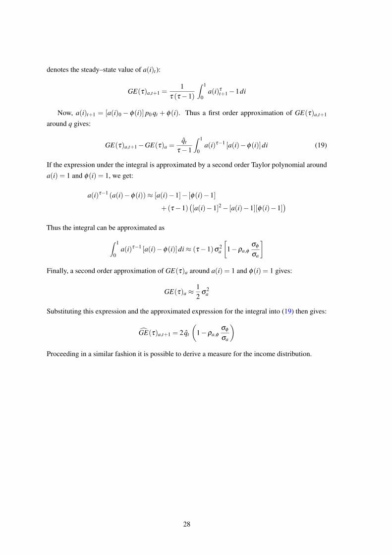
denotes the steady–state value of a(i)t):

GE(τ)a,t+1 =1

τ (τ−1)

∫ 1

0a(i)τ

t+1−1di

Now, a(i)t+1 = [a(i)0− φ(i)] p0 qt + φ(i). Thus a first order approximation of GE(τ)a,t+1

around q gives:

GE(τ)a,t+1−GE(τ)a =qt

τ−1

∫ 1

0a(i)τ−1 [a(i)−φ(i)]di (19)

If the expression under the integral is approximated by a second order Taylor polynomial around

a(i) = 1 and φ(i) = 1, we get:

a(i)τ−1 (a(i)−φ(i))≈ [a(i)−1]− [φ(i)−1]

+ (τ−1)([a(i)−1]2− [a(i)−1][φ(i)−1]

)Thus the integral can be approximated as

∫ 1

0a(i)τ−1 [a(i)−φ(i)]di≈ (τ−1)σ

2a

[1−ρa,φ

σφ

σa

]Finally, a second order approximation of GE(τ)a around a(i) = 1 and φ(i) = 1 gives:

GE(τ)a ≈12

σ2a

Substituting this expression and the approximated expression for the integral into (19) then gives:

GE(τ)a,t+1 = 2 qt

(1−ρa,φ

σφ

σa

)Proceeding in a similar fashion it is possible to derive a measure for the income distribution.

28