18 (Suppl 1-M2) - pdfs.semanticscholar.org · 18 The Open Thermodynamics Journal, 2011, 5, (Suppl...

18 The Open Thermodynamics Journal, 2011, 5, (Suppl 1-M2) 18-28

1874-396X/11 2011 Bentham Open

Open Access

Some Observations Regarding the SAFT-VR-Mie Equation of State

Vladimir Kalikhman1,2, Daniel Kost2 and Ilya Polishuk1,*

1Department of Chemical Engineering & Biotechnology, Ariel University Center, 40700, Ariel, Israel

2Department of Chemistry, Ben-Gurion University of the Negev, Beer-Sheva, 84105, Israel

Abstract: This study demonstrates that the advanced theoretical basis and the consequential numerical complexity do not always guarantee the success of EOS models in predicting the experimental thermodynamic property data. Although one of the best versions of SAFT, namely SAFT-VR-Mie might have doubtless advantages in predicting the data of non-spherical molecules, once again it is shown that there is a price to pay for the excessive model’s complexity. In particular, the present study reveals a previously unnoticed kind of numerical pitfalls, yet generated by the chain term of the SAFT-VR-Mie EOS. A possible way of avoiding the numerical pitfall under consideration is proposed.

Keywords: Equation of state, statistical association fluid theory, high pressure, phase equilibria, sound velocity, heat capacity.

INTRODUCTION

Equations of State (EoS) based on the Statistical Association Fluid Theory (SAFT) present a new generation of fluid phase models offering doubtless advantages over the popular cubic equations [1-5]. The SAFT with attractive potentials of Variable Range and Mie’s monomer hard-core potential (SAFT-VR-Mie) [6] is one of the most successful versions of SAFT due to its advantages in predicting the auxiliary properties [7-10]. In addition, previously [11] it has been concluded that SAFT-VR-Mie is free of the fictitious phase equilibria numerical pitfall characteristic for several other versions of SAFT [12-15]. The current study aims answering two questions:

1 Is the success of SAFT-VR-Mie achieved thanks to its advanced theoretical basis or rather the appropriate parameters fitting?

2 Is this model indeed entirely free of numerical pitfalls?

Since the expression of SAFT-VR-Mie is sophisticated, some possible printing errors have appeared in the previous publications. Therefore it seems worthwhile to provide here its brief description.

THEORY

For the non-polar compounds SAFT models present the residual Helmholtz’s energy as a sum of the following contributions:

Ares= AHS

+ Adisp+ Achain (1)

The hard-sphere (HS) contribution is given as follows:

*Address correspondence to this author at the Department of Chemical Engineering & Biotechnology, Ariel University Center, 40700, Ariel, Israel; Tel: +972-3-9066346; Fax: +972-3-9066323; E-mails: [email protected], [email protected]

AHS= mRT

4 3 2

(1 )2 (2)

where the packing fraction:

=NAv

6 Vm 3 (T ) (3)

NAv is the Avogadro's number, m is the effective number

of segments, is the Lennard-Jones's segment diameter.

Both m and are the model’s adjustable parameters. According to SAFT-VR-Mie [6]:

(T ) =

0.995438 - 0.0259917 T k( ) +

0.00392254 T k( )2

- 0.000289398 T k( )3

3

(4)

is the inter-segment interaction's dispersion energy, k

is the Boltzmann's constant. k is the 3rd model’s adjustable

parameter. It should be pointed out that the References [7-9] have used instead of Equation (4) the numerically calculated integral definition, a technique which is not completely clear to us. Nevertheless, it should be pointed out that since we were able to exactly reproduce all the results of the Reference [7], implementation of Equation (4) seems justified. Moreover, the temperature dependence of has

no impact on the numerical pitfall discussed below.

The SAFT-VR-Mie’s dispersion contribution is given as:

Adisp= mRT a1

M+

2a2M( ) (5)

where

=1

kT (6)

The first perturbation term used in the previous study is given as:

Some Observations Regarding the SAFT-VR-Mie Equation of State The Open Thermodynamics Journal, 2011, Volume 5 19

a1M

= C a1S ( 1 ) a1

S ( 2 ) (7)

1 is typically equal to 6 and 2 is the 4th model’s

adjustable parameters. The second perturbation term is:

a2M

=C

2

1( )4

1+ 4 + 4 2

a1S (2 1)

(8)

The expression corresponding to the mean attractive energy for a Sutherland- system is:

a1S ( X ) = 4

3

i 3

1 eff / 2

(1 eff )3

X=1,2

(9)

and the effective packing fraction is defined as:

eff ( X ) = c1 + c22 (10)

while c1 and c2 are given by the following matrix:

c1

c2

=

0.943973 0.422543 0.0371763 0.00116901

0.370942 0.173333 0.0175599 0.000572729

1

X

X

2

X

3

X=1,2

(11)

a1S (2 1) in Equation (8) means than 1 in Equations

(9-11) is replaced by 2 1 .

And, finally,

C =2

2 1

2

1

1/( 2 1 )

(12)

Some confusion appears concerning the SAFT- VR-Mie’s chain contribution. In particular, in the Reference [7] it is given as:

Achain= RT (1 m) ln

1 21( )

3 +4

a1M C 1

4a1

S ( 1 ) +C 2

4a2

S ( 2 ) (13a)

In the Reference [9] the last term of the expression above appears as:

Achain= RT (1 m) ln

1 21( )

3 +4

a1M C 1

4a1

S ( 1 ) +C 2

4a1

S ( 2 ) (13b)

Unfortunately, both equations (13a) and (13b) do not yield accurate modeling of data with the parameters listed in Reference [7]. However we were able to exactly reproduce the results of the Reference [7] with:

Achain= RT (1 m) ln

1 21( )

3 +4

a1M C 1

3a1

S ( 1 ) +C 2

3a1

S ( 2 ) (13c)

It should be pointed out that substitution Equations (6)-(12) into Equations (5) and (13) results in the particularly long and complicated expressions. In the current study the performance of SAFT-VR-Mie is compared with the much simpler version of SAFT, namely the original SAFT of Chapman et al. [16]. This version implements the same

expression for AHS however:

(T ) =1+ 0.2977 k( )T

1+ 0.33163 k( )T + 0.0010477 + 0.025337m 1

mk( )

2

T 2

3

(14)

Adisp= mR k( ) a1

M+

a2M

k( )T

(15)

The original Chapman’s et al. [16] expressions for a1M

and a2M might be reduced to:

a1M

=3 2

8.5959 6.1344 2 3.87882 3+ 25.3316 4 (16)

a2M

=3 2

1.9075 +13.4675 2 40.5171 3+ 39.1711 4 (17)

and the chain term [16] is given as:

Achain= RT (1 m) ln

1 2

1( )3 (18)

Having the expression for Ares , the pressure is obtained as:

P =RT

V

Ares

vT

(19)

The residual heat capacities might be calculated using the following relationships:

CVres

= TAres2

2Tv

(20)

CPres

= CVres R T

PT( )

v

2

Pv( )

T

(21)

The values of CV and CP are obtained by adding the

pertinent ideal gas properties available in the literature [17]. The sound velocities, enthalpies, entropies and the virial coefficients might be evaluated with:

W =CP

CV

v2

Mw

P

v T

(22)

H res= RT T

Ares

RT( )T

v

+Pv

RT1 (23)

20 The Open Thermodynamics Journal, 2011, Volume 5 Kalikhman et al.

Sres= R T

Ares

RT( )T

v

Ares

RT+ ln

Pv

RT (24)

B = Lim0

Z

T

(25)

C =

Lim0

Z 2

2

T

2 (26)

The calculations have been performed using the Mathematica 7® software (the pertinent routines can be obtained from the corresponding author by request).

RESULTS

In order to evaluate the contribution of the very sophisticated Equations (5) and (13) to the accuracy of SAFT-VR-Mie let as compare its performance with the much simpler original Chapman’s et al. SAFT [16]. With the purpose of reducing the effect of the parameters fitting the following strategy is proposed:

1 The equal values of the parameters m and for both SAFTs are taken from the reference [7]. Then the nearly equal contributions of the HS terms are obtained and the deviations are originated mainly by the differences in the dispersion and the chain terms.

2 The Chapman et al. SAFT’s k is fitted to the critical

temperature yielded by SAFT-VR-Mie in order to

achieve similarity between the phase envelopes predicted by both models.

Thus for methane the Chapman et al. SAFT’s parameters

are: m = 1, = 3.7332 Å and k = 147.736 K. The values of

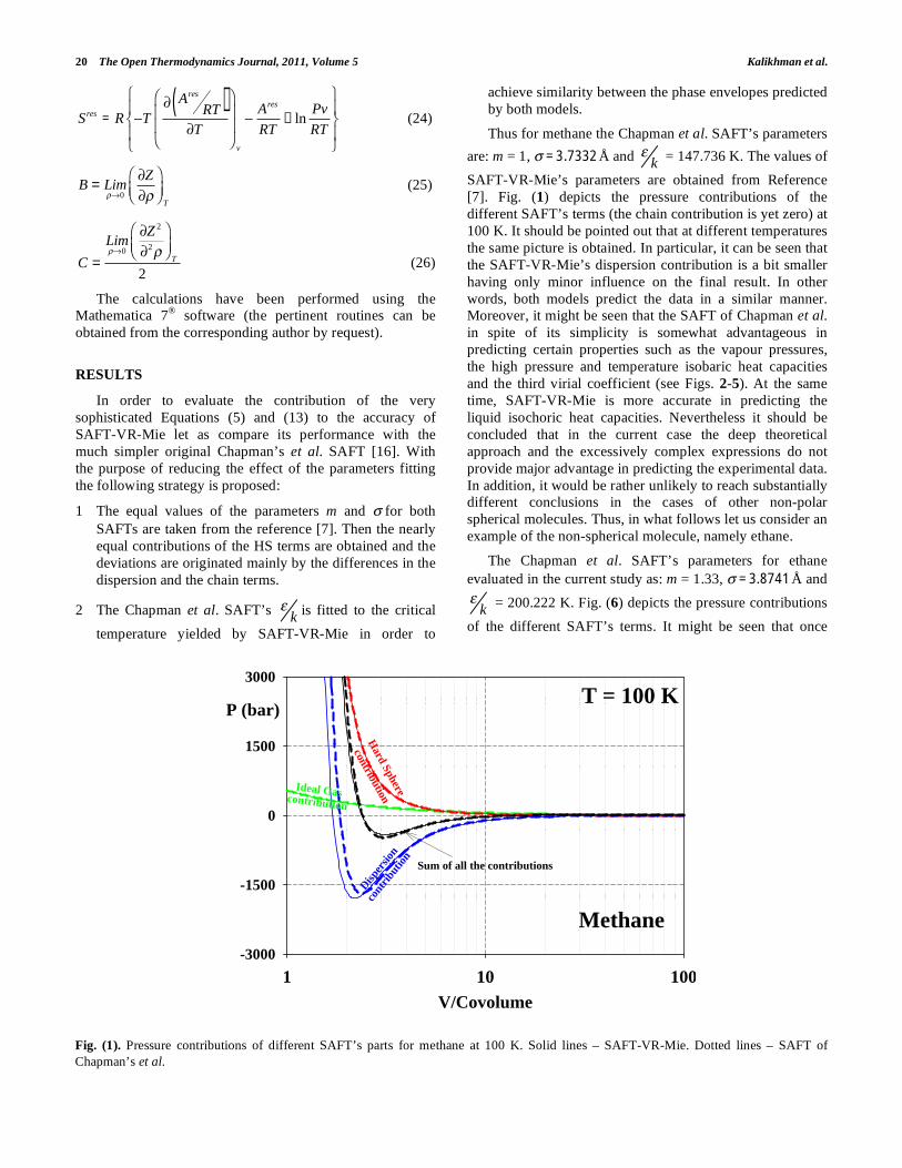
SAFT-VR-Mie’s parameters are obtained from Reference [7]. Fig. (1) depicts the pressure contributions of the different SAFT’s terms (the chain contribution is yet zero) at 100 K. It should be pointed out that at different temperatures the same picture is obtained. In particular, it can be seen that the SAFT-VR-Mie’s dispersion contribution is a bit smaller having only minor influence on the final result. In other words, both models predict the data in a similar manner. Moreover, it might be seen that the SAFT of Chapman et al. in spite of its simplicity is somewhat advantageous in predicting certain properties such as the vapour pressures, the high pressure and temperature isobaric heat capacities and the third virial coefficient (see Figs. 2-5). At the same time, SAFT-VR-Mie is more accurate in predicting the liquid isochoric heat capacities. Nevertheless it should be concluded that in the current case the deep theoretical approach and the excessively complex expressions do not provide major advantage in predicting the experimental data. In addition, it would be rather unlikely to reach substantially different conclusions in the cases of other non-polar spherical molecules. Thus, in what follows let us consider an example of the non-spherical molecule, namely ethane.

The Chapman et al. SAFT’s parameters for ethane evaluated in the current study as: m = 1.33, = 3.8741 Å and

k = 200.222 K. Fig. (6) depicts the pressure contributions

of the different SAFT’s terms. It might be seen that once

Fig. (1). Pressure contributions of different SAFT’s parts for methane at 100 K. Solid lines – SAFT-VR-Mie. Dotted lines – SAFT of Chapman’s et al.

V/Covolume

1 10 100-3000

-1500

0

1500

3000

P (bar)

Methane

Ideal Gascontribution

Hard Sphere

contribution

Disper

sion

cont

ribut

ion

T = 100 K

Sum of all the contributions


Fig. (2). Vapor pressure, enthalpy and entropy of condensation of methane. – experimental data [18]. Solid lines – SAFT-VR-Mie; dotted lines – SAFT of Chapman et al.

Fig. (3). Coexisting densities, speeds of sound, isochoric and isobaric heat capacities of methane. Experimental data [18]: – liquid phase,

– vapor phase. Solid lines – SAFT-VR-Mie; dotted lines – SAFT of Chapman et al.

T (K)100 130 160 190

0

20

40

60

80

P (bar) Vapor pressure

H (J/mol)-10000 -8000 -6000 -4000 -2000 0

90

120

150

180

210

T (K)

Heat of condensation

S (J/mol)-100 -80 -60 -40 -20 0

90

120

150

180

210

T (K)

Entropy of condensation

(g/m3)0 100 200 300 400 500

90

120

150

180

210

T (K)

Coexisting densities

W (m/s)400 800 1200 1600

90

120

150

180

210

T (K) Coexisting speeds of sound

Cv (J/gmol-K)20 30 40 50 60

90

120

150

180

210

T (K)

Coexisting isohoric heat capacities

Cp (J/gmol-K)30 50 70 90

90

120

150

180

210

T (K)



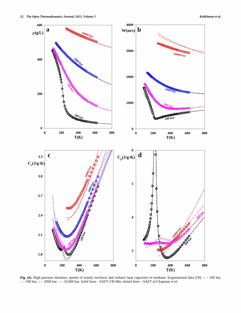
Fig. (4). High pressure densities, speeds of sound, isochoric and isobaric heat capacities of methane. Experimental data [18]: – 100 bar, – 500 bar, – 2000 bar, – 10,000 bar. Solid lines – SAFT-VR-Mie; dotted lines – SAFT of Chapman et al.

T(K)0 200 400 600 800

0

200

400

600

(g/L)a

10000 bar

2000 bar

500 bar

100 bar

T(K)0 200 400 600 800

0

1000

2000

3000

4000

W(m/s) b

10000 bar

2000 bar

100 bar

500 bar

T(K)0 200 400 600 800

1.8

2.1

2.4

2.7

3.0

3.3

Cv(J/g-K)

c

1000

0 ba

r20

00 b

ar

100

bar

500

bar

T(K)0 200 400 600 800

3

4

5

6

Cp(J/g-K) d

1000

0 ba

r

100

bar

500

bar


Fig. (5). Virial coefficients and Joule-Thomson inversion curve of methane. – experimental data [17,19,20]. Solid lines – SAFT-VR-Mie; dotted lines – SAFT of Chapman et al.

Fig. (6). Pressure contributions of different SAFT’s parts for ethane at 150-153 K. Solid lines – SAFT-VR-Mie. Dotted lines – SAFT of Chapman’s et al.

T(K)200 400 600 800 1000

-.5

-.4

-.3

-.2

-.1

0.0

.1

B (L/mol) Methane

200 400 600 800 10000.000

.002

.004

.006

T(K)

C(L/mol)2

Methane

Tr.5 2.0 3.5 5.0

0.0

3.5

7.0

10.5

14.0

Pr

Joule-Thom

son Inversion Curve

Methane

V/Covolume

1 10 100-3000

-1500

0

1500

3000

P (bar)

Ethane


Hard Sphere

contribution

Disper

sion

cont

ribut

ion

T = 153 K


Chain contribution

V/Covolume

1 10 100-3000

-1500

0

1500

3000

P (bar)

Ethane


Hard Sphere

contribution

Disp

ersio

n

cont

ribut

ion

T = 152 K


Chain contribution

V/Covolume

1 10 100-3000

-1500

0

1500

3000

P (bar)

Ethane


Hard Sphere

contribution

Disp

ersioncon

tribu

tion

T = 151 K


Chain contribution

V/Covolume

1 10 100-3000

-1500

0

1500

3000

P (bar)

Ethane


Hard S

phere

contribution

Dispersion

contrib

ution

T = 150 K


Chain contribution


Fig. (7). Vapor pressure, enthalpy and entropy of condensation of ethane. – experimental data [21]. Solid lines – SAFT-VR-Mie; dotted lines – SAFT of Chapman et al.

Fig. (8). Coexisting densities, speeds of sound, isochoric and isobaric heat capacities of ethane. Experimental data [21]: – liquid phase, – vapor phase. Solid lines – SAFT-VR-Mie; dotted lines – SAFT of Chapman et al.

T (K)90 150 210 270 330

0

20

40

60

80

P (bar) Vapor pressure

H (J/mol)-20000 -16000 -12000 -8000 -4000 0

90

150

210

270

330

T (K)

Heat of condensation

S (J/mol)-160 -140 -120 -100 -80 -60 -40 -20 0

90

150

210

270

330

T (K)

Entropy of condensation

(g/m3)0 100 200 300 400 500 600 700

90

150

210

270

330

T (K)

Coexisting densities

W (m/s)0 500 1000 1500 2000

90

150

210

270

330

T (K) Coexisting speeds of sound

Cv (J/gmol-K)-20 0 20 40 60 80

90

150

210

270

330

T (K) Coexisting isohoric heat capacities

Cp (J/gmol-K)30 50 70 90 110

90

150

210

270

330

T (K)



more the HS contributions of both models are nearly identical and the SAFT-VR-Mie’s dispersion contribution is a bit smaller. However the chain term yet yields some unexpected results. The figure demonstrates development of the previously unnoticed numerical pitfall behaviour. In particular, it might be seen that the SAFT-VR-Mie’s chain term at certain temperatures might generate an additional fictitious covolume and the artificial phase instability. As a

result, the model might predict the negative values of the isochoric heat capacities and the unrealistic results for sound velocities (see Figs. 8, 9). At the same time, outside the numerical failure region, the SAFT-VR-Mie’s chain term contributes to a better estimation of data. In particular, Figs. (6-10) demonstrate its over-all advantage over the SAFT of Chapman et al. at the temperatures above ~200 K.

Fig. (9). High pressure densities, speeds of sound, isochoric and isobaric heat capacities of ethane. Experimental data [21]: – 100 bar, – 500 bar, – 2000 bar, – 9000 bar. Solid lines – SAFT-VR-Mie; dotted lines – SAFT of Chapman et al.

T(K)0 200 400 600 800

0

200

400

600

800

(g/L)a

9000 bar

2000 bar

500 bar

100 bar

T(K)0 200 400 600 800

0

1000

2000

3000

4000

W(m/s) b

9000 bar

2000 bar

100 bar

500 bar

T(K)0 200 400 600 800

1.2

1.5

1.8

2.1

2.4

2.7

3.0

3.3

Cv(J/g-K)

c

9000

bar

2000

bar

100

bar

500 bar

0 200 400 600 800

-.8

0.0

.8

1.6

2.4

3.2

T(K)0 200 400 600 800

2

3

4

5

Cp(J/g-K) d

9000

bar

100

bar

500

bar


Numerical analysis of Equation (13c) indicates that the numerical pitfall described above is caused by an artificial covolume generated by its last term and it does not seem to be related to the theoretical background of the model [22]. This numerical pitfall might easily be removed by reducing the numerical value of the last term of Equation (13c), for example as follows:

Achain= RT (1 m) ln

1 21( )

3 +4

a1M C 1

3a1

S ( 1 ) +3C 2

10a1

S ( 2 ) (27)

Implementation of Equation (27) instead of Equation (13c) makes the results of SAFT-VR-Mie remarkable similar to the SAFT of Chapman et al.

CONCLUSIONS

This study demonstrates that the advanced theoretical basis and the consequential numerical complexity do not always guarantee the success of EOS models in predicting the experimental thermodynamic property data. In particular,

it is demonstrated that the predictive capabilities of the advanced version of SAFT, namely SAFT-VR-Mie in the case of the spherical non-polar molecules such as methane might in fact be similar to the modeling capacity of the much simpler version of SAFT, namely the SAFT of Chapman et al. Although SAFT-VR-Mie might have a doubtless advantage in predicting the data of non-spherical molecules, once again there is a price to pay for the excessive model’s complexity. In particular, such complexity might result in appearance of undesired numerical pitfalls. Thus the present study reveals a previously unnoticed kind of numerical pitfalls, yet generated by the chain term of the SAFT-VR-Mie EOS. A possible way of avoiding the numerical pitfall under consideration is proposed.

CONFLICT OF INTEREST

None declared.

ACKNOWLEDGMENTS

Acknowledgment is made to the Donors of the American Chemical Society Petroleum Research Fund for support of this research, grant N° PRF#47338-B6.

Fig. (10). Virial coefficients and Joule-Thomson inversion curve of ethane. – experimental data [17,19,20]. Solid lines – SAFT-VR-Mie; dotted lines – SAFT of Chapman et al.

T(K)0 200 400 600 800 1000-1.0

-.8

-.6

-.4

-.2

0.0

B (L/mol)

Ethane

200 400 600 800 1000

0.000

.004

.008

.012

.016

T(K)

C (L/mol)2

Ethane

Tr.5 2.0 3.5 5.0

0.0

3.5

7.0

10.5

14.0

Pr

Joule-Thom

son Inversion Curve

Ethane


SYMBOLS

A = Helmholtz free energy

B = Second virial coefficient

C = Third virial coefficient

CV = Isochoric heat capacity

CP = Isobaric heat capacity

m = Effective number of segments

H = Enthalpy

Mw = Molecular weight

NAv = Avogadro's number

P = Pressure

R = Universal gas constant

S = Entropy

T = Temperature

v = Molar volume

W = Speed of sound

Z = Compressibility

Greek letters

1, 2 = Coefficients of the Mie’s potential

= Reduced density

/k = Segment energy parameter divided by Boltzmann's constant

(T) = Temperature dependence of reduced density

= Density

= Lennard-Jones temperature-independent segment diameter (Å)

Subscripts

c = Critical state

Superscripts

res = Residual property

Abbreviations

EOS = Equation of state

HS = Hard sphere

SAFT = Statistical association fluid theory

REFERENCES

[1] Y. S. Wei, R. J. Sadus, “Equations of state for the calculation of fluid-phase equilibria”, AIChE J., vol. 46, pp. 169-196, January 2000.

[2] E. A. Müller, K. E. Gubbins, “Molecular-based equations of state for associating fluids: a review of SAFT and related approaches”, Ind. Eng. Chem. Res., vol. 40, pp. 2193-2211, July 2001.

[3] I. G. Economou, “Statistical associating fluid theory: a successful model for the calculation of thermodynamic and phase equilibrium properties of complex fluid mixtures”, Ind. Eng. Chem. Res., vol. 41, pp. 953-962, March 2002.

[4] S. P. Tan, H. Adidharma, M. Radosz, “Recent advances and applications of statistical associating fluid theory”, Ind. Eng.

Chem. Res., vol. 47, pp. 8063-8082, December 2008. [5] G. M. Kontogeorgis, G. K. Folas, Thermodynamic Models for

Industrial Applications. From Classical and Advanced Mixing

Rules to Association Theories. New York: John Wiley & Sons, 2010.

[6] A. Gil-Villegas, A. Galindo, P. J. Whitehead, S. J. Mills, G. Jackson, A. N. Burgess, “Statistical associating fluid theory for chain molecules with attractive potentials of variable range”, J.

Chem. Phys., vol. 106, pp. 4168-4186, March 1997. [7] T. Lafitte, D. Bessières, M. M. Piñeiro, J.-L. Daridon,

“Simultaneous estimation of phase behavior and second-derivative properties using the statistical associating fluid theory with variable range approach”, J. Chem. Phys., vol. 124, pp. 024509/1-16, January 2006.

[8] T. Lafitte, M. M. Piñeiro, J.-L. Daridon, D. Bessières, “A comprehensive description of chemical association effects on second derivative properties of alcohols through a SAFT-VR approach”, J. Phys. Chem. B, vol. 111, pp. 3447-3461, March 2007.

[9] T. Lafitte, F. Plantier, M. M. Piñeiro, J.-L. Daridon, D. Bessières, “Accurate global thermophysical characterization of hydro- fluoroethers through a statistical associating fluid theory variable range approach, based on new experimental high-pressure volumetric and acoustic data”, Ind. Eng. Chem. Res., vol. 46, pp. 6998-7007, June 2007.

[10] M. Khammar, J. Shaw, “Speed of sound prediction in 1-n-alcohol+ n-alkane mixtures using a translated SAFT-VR-Mie equation of state”, Fluid Phase Equilib., vol. 288, pp. 145-154, January 2010.

[11] I. Polishuk, “Addressing the issue of numerical pitfalls characteristic for SAFT EOS models”, Fluid Phase Equilib., vol. 301, pp. 123-129, January 2011.

[12] N. Koak, Th. W. de Loos, R. A. Heidemann, “Effect of the power series dispersion term on the pressure-volume behavior of statistical associating fluid theory”, Ind. Eng. Chem. Res., vol. 38, pp. 1718-1722, February 1999.

[13] L.Yelash, M. Müller, W. Paul, K. Binder, “A global investigation of phase equilibria using the perturbed-chain statistical-associating-fluid-theory approach”, J. Chem. Phys., vol. 123, pp. 14908/1-15, July 2005.

[14] R. Privat, R. Gani, J.-N. Jaubert, “Are safe results obtained when the PC-SAFT equation of state is applied to ordinary pure chemicals?” Fluid Phase Equilib., vol. 295, pp. 76-92, August 2010.

[15] I. Polishuk, “About the numerical pitfalls characteristic for SAFT EOS models”, Fluid Phase Equilib. vol. 298, pp. 67-74, November 2010.

[16] W. G. Chapman, K. E. Gubbins, G. Jackson, M. Radosz, “New reference equation of state for associating liquids”, Ind. Eng.

Chem. Res., vol. 29, pp. 1709-1721, February 1990. [17] R. L. Rowley, W. V. Wilding, T. E. Daubert, R. P. Danner, M.E.

Adams, Physical and Thermodynamic Properties of Pure

Chemicals: DIPPR: Data Compilation. New-York: Taylor & Francis, 2010.

[18] U. Setzmann, W. Wagner, “A new equation of state and tables of thermodynamic properties for methane covering the range from 'the melting line to 625 K at pressures up to 1000 MPa”, J. Phys.

Chem. Ref. Data, vol. 20, pp. 1061-1155, June 1991. [19] D. W. Green, R. H. Perry, Perry's Chemical Engineers' Handbook

(8th Edition). New-York: McGraw-Hill, 2008. [20] J. H. Dymond, K. N. Marsh, R. C. Wilhoit, K. C. Wong, Virial

Coefficients of Pure Gases and Mixtures. Landolt-Börnstein


Numerical Data and Functional Relationships in Science and

Technology New Series Group IV: Physical Chemistry Vol. 21.

Berlin: Springer-Verlag, 2002. [21] D. Bücker, W. Wagner, “A reference equation of state for the

thermodynamic properties of ethane for temperatures from the melting line to 675 K and pressures up to 900 MPa”, J. Phys.

Chem. Ref. Data, vol. 35, pp. 205-266, January 2006.

[22] G. Galliero, T. Lafitte, D. Bessieres, C. Boned, “Thermodynamic properties of the Mie n-6 fluid: A comparison between statistical associating fluid theory of variable range approach and molecular dynamics results”, J. Chem. Phys., vol. 127, pp. 184506/1-184506/12, May 2007.

Received: March 22, 2011 Revised: July 26, 2011 Accepted: August 30, 2011

© Kalikhman et al.; Licensee Bentham Open.

This is an open access article licensed under the terms of the Creative Commons Attribution Non-Commercial License (http://creativecommons.org/licenses/by-nc/3.0/) which permits unrestricted, non-commercial use, distribution and reproduction in any medium, provided the work is properly cited.

18 (Suppl 1-M2) - pdfs.semanticscholar.org · 18 The Open Thermodynamics Journal, 2011, 5, (Suppl...

Documents

Transcript of 18 (Suppl 1-M2) - pdfs.semanticscholar.org · 18 The Open Thermodynamics Journal, 2011, 5, (Suppl...