Queuing systems: Modeling, analysis and simulation - CiteSeerX
543
18
Design & Implementation of
Service and Queuing Systems
"If you think you have reservations, you're at the wrong place."
-Sign in Ed Debevec's Restaurant
18.1 Introduction The distinctive feature of a service system is that it cannot stock its product in anticipation of
impending demand. An organization whose main product is a service can prepare for increased
demand only by increasing its capacity. A major question in planning a service system is capacity
sizing. How many cashiers, ticket takers, staffers at a toll plaza, phone lines, computers at an internet
service provider, runways at an airport, tables at a restaurant, fire stations, beds in a hospital, police
cars in a region, restroom facilities, elevators, or machine maintenance personnel are needed so as to
provide acceptable service?
Capacity planning for a service facility involves three steps:
1. Data collection. Assemble all relevant historical data or set up a system for the on-going
collection of demand data.
2. Data analysis. Forecast demand; ascertain the probabilistic components of the demand;
determine the minimum acceptable capacity for each demand period.
3. Requirements recommendation. Taking into account such factors as the probabilistic
nature of demand, cost of poorly served demand, capacity change costs and standard
work shift patterns, recommend a capacity plan that minimizes all relevant expected
costs.
18.2 Forecasting Demand for Services Standard forecasting methods apply as well to demand for services as to the demand for goods.
Long-range forecasting of demand for services must incorporate the fact that demand for services does
not react to changes in the health of the economy in the same way as demand for goods. For example,
demand for goods such as food is relatively unaffected by the health of the economy; whereas, demand
for luxury services such as restaurant dining tends to be diminished by economic recessions. Demand
for fast food dining service has been increased by the advent of the working mother.

544 Chapter 18 Queuing Systems
Shorter range forecasting of the demand for services is concerned in large part with the
measurement of the cyclical components of demand. In particular, one wants to identify (say for a
service that processes phone calls) the:
- hour of the day effect,
- day of the week effect (e.g., the number of calls per day to the 911 emergency number in
New York City has been found to vary somewhat predictably almost by a factor of two
based on the day of the week),
- week of year effect,
- moveable feast effect (e.g., Mother's Day, Labor Day, Easter, etc),
- advertising promotions.
18.3 Waiting Line or Queuing Theory Queuing theory is a well-developed branch of probability theory that has long been used in the
telephone industry to aid capacity planning. A. K. Erlang performed the first serious analysis of
waiting lines or queues for the Copenhagen telephone system in the early 20th century. Erlang's
methods are still widely used today in the telephone industry for setting various capacities such as
operator staffing levels. For application at the mail order firm, L.L. Bean, see Andrews and Parsons
(1993). Gaballa and Pearce (1979) describe applications at Qantas Airline. An important recent
application of queuing models is in telephone call centers. There are two kinds of call centers: 1) In-
bound call centers that handle incoming calls, such as orders for a catalog company, or customer
support for a product; and 2) Out-bound call centers where telephones place calls to prospective
customers to solicit business, or perhaps to remind current customers to pay their bills.
It is useful to note that a waiting line or queue is usually the negative of an inventory. Stock
carried in inventory allows an arriving customer to be immediately satisfied. When the inventory is
depleted, customers must wait until units of product arrive. The backlogged or waiting customers
constitute a negative inventory, but they can also be thought of as a queue. A more explicit example is
a taxi stand. Sometimes taxi cabs will be in line at the stand waiting for customers. At other times,
customers may be in line waiting for cabs. What you consider a queue and what you consider an
inventory depends upon whether you are a cab driver or a cab customer.
In queuing theory, a service system has three components:
1) an arrival process,
2) a queue discipline, and
3) a service process.
The figure below illustrates:
Arrival Process Queue discipline Service Process
(e.g., One
arrival every 7
minutes on
average.)
(e.g., First-come
first-serve), but
if 10 are waiting,
then arrivals are
lost.
(e.g., 3 identical
servers). Mean
service time is 9
minutes.
A good introduction to queuing theory can be found in Gross and Harris (1998).

Queuing Systems Chapter 18 545
18.3.1 Arrival Process We distinguish between two types of arrival process: i) finite source and ii) infinite source. An
example of finite source is 10 machines being watched over by a single repair person. When a machine
breaks down, it corresponds to the arrival of a customer. The number of broken down machines
awaiting repair is the number of waiting customers. We would say this system has a finite source of
size ten. With a finite population, the arrival rate is reduced as more customers enter the system. When
there are already 8 of 10 machines waiting for repairs or being repaired, then the arrival rate of further
customers (broken machines) is only 2/10 of the arrival rate if all the machines were up and running
and thus eligible to breakdown.
An airline telephone reservation system, on the other hand, would typically be considered as
having an infinite calling population. With an infinite population, the arrival rate is unaffected by the
number of customers already in the system.
In addition to the type of arrival process, a second piece of information we need to supply is the
mean time between calls. If the calling population is infinite, then this is a single number independent
of the service process. However, for a finite population, there is a possibility for ambiguity because the
arrival rate at any moment depends upon the number waiting. The ambiguity is resolved by
concentrating on only one of the supposedly identical customers. It is sufficient to specify the mean
time until a given customer generates another call, given that he just completed service. We call this
the mean time between failures or MTBF for short.
A fine point that we are glossing over is the question of the distribution (as opposed to the mean)
of the time between calls. Two situations may have the same mean time between calls, but radically
different distributions. For example, suppose that in situation 1 every interval between calls is exactly
10 minutes, while, in situation 2, 10% of the intervals are 1 minute long and 90% of the intervals are
11 minutes. Both have the same mean, but it seems plausible that system 2 will be more erratic and
will incur more waiting time. The standard assumption is that the distribution of the time between calls
is the so-called exponential. Happily, it appears that this assumption is not far off the mark for most
real situations.
The exponential distribution plays a key role in the models we will consider. For the infinite
source case, we assume that the times between successive arrivals are distributed according to the
exponential distribution. An exponential density function is graphed in the figure 18.1:
Figure 18.1. An exponential distribution with mean 2.
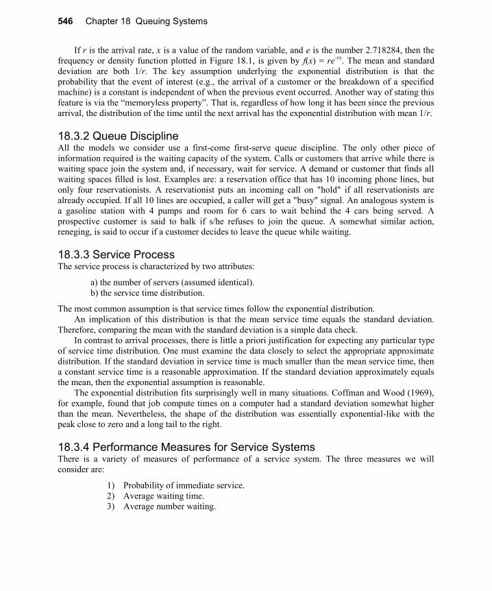
546 Chapter 18 Queuing Systems
If r is the arrival rate, x is a value of the random variable, and e is the number 2.718284, then the
frequency or density function plotted in Figure 18.1, is given by f(x) = re-rx
. The mean and standard
deviation are both 1/r. The key assumption underlying the exponential distribution is that the
probability that the event of interest (e.g., the arrival of a customer or the breakdown of a specified
machine) is a constant is independent of when the previous event occurred. Another way of stating this
feature is via the “memoryless property”. That is, regardless of how long it has been since the previous
arrival, the distribution of the time until the next arrival has the exponential distribution with mean 1/r.
18.3.2 Queue Discipline All the models we consider use a first-come first-serve queue discipline. The only other piece of
information required is the waiting capacity of the system. Calls or customers that arrive while there is
waiting space join the system and, if necessary, wait for service. A demand or customer that finds all
waiting spaces filled is lost. Examples are: a reservation office that has 10 incoming phone lines, but
only four reservationists. A reservationist puts an incoming call on "hold" if all reservationists are
already occupied. If all 10 lines are occupied, a caller will get a "busy" signal. An analogous system is
a gasoline station with 4 pumps and room for 6 cars to wait behind the 4 cars being served. A
prospective customer is said to balk if s/he refuses to join the queue. A somewhat similar action,
reneging, is said to occur if a customer decides to leave the queue while waiting.
18.3.3 Service Process The service process is characterized by two attributes:
a) the number of servers (assumed identical).
b) the service time distribution.
The most common assumption is that service times follow the exponential distribution.
An implication of this distribution is that the mean service time equals the standard deviation.
Therefore, comparing the mean with the standard deviation is a simple data check.
In contrast to arrival processes, there is little a priori justification for expecting any particular type
of service time distribution. One must examine the data closely to select the appropriate approximate
distribution. If the standard deviation in service time is much smaller than the mean service time, then
a constant service time is a reasonable approximation. If the standard deviation approximately equals
the mean, then the exponential assumption is reasonable.
The exponential distribution fits surprisingly well in many situations. Coffman and Wood (1969),
for example, found that job compute times on a computer had a standard deviation somewhat higher
than the mean. Nevertheless, the shape of the distribution was essentially exponential-like with the
peak close to zero and a long tail to the right.
18.3.4 Performance Measures for Service Systems There is a variety of measures of performance of a service system. The three measures we will
consider are:
1) Probability of immediate service.
2) Average waiting time.
3) Average number waiting.

Queuing Systems Chapter 18 547
18.3.5 Stationarity In general, queuing models assume that demand is stationary (i.e., stable over time) or that the system
has reached steady state. Obviously, this cannot be true if demand is spread over a sufficiently long
period of time (e.g., an entire day). For example, it is usually obvious that the mean time between
phone calls at 11:00 a.m. on any given day is not the same as the mean time at 11:00 p.m. of that same
day. We define the load on a service system as the product of the mean arrival rate times the means
service time per customer. Load is a unit-less quantity, which is a lower bound on the number of
servers one would need to process the arriving work without having the queue grow without bound.
We should probably be careful about using a steady-state-based queuing model if load is not constant
for a reasonably long interval. What constitutes a “reasonable long interval”? To answer that question,
let us define a notation we will use henceforth:
R = mean arrival rate,
T = mean or expected service time,
S = number of servers.
The quantity T/(S – R*T) is a simple definition of “a reasonably long interval”. Notice that it
becomes unbounded as the load approaches S.
18.3.6 A Handy Little Formula There is a very simple yet general relationship between the average number in system and the average
time in system. In inventory circles, this relationship is known as the inventory turns equation. In the
service or queuing world, it is known as Little's Flow Equation, see Little (1961). In words, Little's
equation is:
(average number in systems) = (arrival rate) * (average time-in-system)
Reworded in inventory terminology, it is:
(average inventory level) = (sales rate) * (average time-in-system)
Inventory managers frequently measure performance in "inventory turns", where:
(inventory turns) = 1/(average time-in-system).
Rearranging the Little's Flow equation:
(average inventory level) = (sales rate)/(inventory turns)
or
(inventory turns) = (sales rate)/(average inventory level)
Little's Equation is very general. The only essential requirement is that the system to which it is
applied cannot be drifting off to infinity. No particular probabilistic assumptions are required.
18.3.7 Example Customers arrive at a rate of 25 per hour on average. Time-in-system averages out to 12 minutes. What
is the average number of customers in system?
Ans. (Average number in system) = (25/hour) * 12 minutes * 1 hour/60 minutes)
= 25 * (1/5) = 5

548 Chapter 18 Queuing Systems
18.4 Solved Queuing Models There are five situations or models that we will consider. They are summarized in Table 1. The key
feature of these situations is that there are fairly simple formulae describing the performance of these
systems.
Table 1:
Solved Service System Models Model
Feature
I
II
III
IV
V
Queue
Notation
(M/G/c/c) (M/M/c) (M/G/) (F/M/c) (M/G/1)
Population
Size
Infinite Infinite Infinite Finite Infinite
Arrival
Process
Poisson Poisson Poisson General Poisson
Waiting
Space
None Infinite Infinite Infinite Infinite
Number
of Servers
Arbitrary Arbitrary Infinite Arbitrary 1
Service
distribution
Arbitrary
/General
Exponential Arbitrary
/General
Exponential Arbitrary
/General
Solve
with
@PEL or B(s,a) @PEB or C(s,a) @PPS or
Poisson
@PFS Formula
The five models are labeled by the notation typically used for them in queuing literature. The
notation is of the form (arrival process/service distribution/number of servers [/number spaces
available] where:
M = exponential (or Markovian) distributed,
G = general or arbitrary,
D = deterministic or fixed, and
F = finite source.
The two “workhorse” models of this set of five are a) the M/G/c/c, also know as the Erlang loss or
Erlang-B model, and b) the M/M/c, also known as the Erlang C model. LINGO has two built-in
functions, @PEL() and @PEB() that “solve” these two cases. Their use is illustrated below.
Queuing Systems Chapter 18 549
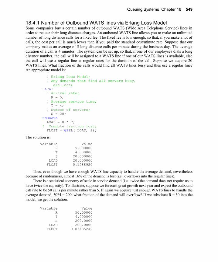
18.4.1 Number of Outbound WATS lines via Erlang Loss Model Some companies buy a certain number of outbound WATS (Wide Area Telephone Service) lines in
order to reduce their long distance charges. An outbound WATS line allows you to make an unlimited
number of long distance calls for a fixed fee. The fixed fee is low enough, so that, if you make a lot of
calls, the cost per call is much lower than if you paid the standard cost/minute rate. Suppose that our
company makes an average of 5 long distance calls per minute during the business day. The average
duration of a call is 4 minutes. The system can be set up, so that, if one of our employees dials a long
distance number, the call will be assigned to a WATS line if one of our WATS lines is available, else
the call will use a regular line at regular rates for the duration of the call. Suppose we acquire 20
WATS lines. What fraction of the calls would find all WATS lines busy and thus use a regular line?
An appropriate model is:
! Erlang Loss Model;
! Any demands that find all servers busy,
are lost;
DATA:
! Arrival rate;
R = 5;
! Average service time;
T = 4;
! Number of servers;
S = 20;
ENDDATA
LOAD = R * T;
! Compute fraction lost;
FLOST = @PEL( LOAD, S);
The solution is:
Variable Value
R 5.000000
T 4.000000
S 20.000000
LOAD 20.000000
FLOST 0.1588920
Thus, even though we have enough WATS line capacity to handle the average demand, nevertheless
because of randomness, almost 16% of the demand is lost (i.e., overflows into the regular lines).
There is a statistical economy of scale in service demand (i.e., twice the demand does not require us to
have twice the capacity). To illustrate, suppose we forecast great growth next year and expect the outbound
call rate to be 50 calls per minute rather than 5. If again we acquire just enough WATS lines to handle the
average demand, 50*4 = 200, what fraction of the demand will overflow? If we substitute R = 50 into the
model, we get the solution:
Variable Value
R 50.00000
T 4.000000
S 200.0000
LOAD 200.0000
FLOST 0.05435242

550 Chapter 18 Queuing Systems
The fraction overflow has dropped to approximately, 5%, even though we are still setting capacity
equal to the average demand.
18.4.2 Evaluating Service Centralization via the Erlang C Model The Ukallus Company takes phone orders at two independent offices and is considering combining the
two into a single office, which can be reached via an "800" number. Both offices have similar volumes
of 50 phone calls per hour (= .83333/minute) handled by 4 order takers in each office. Each office has
sufficient incoming lines that automatically queue calls until an order taker is available. The time to
process a call is exponentially distributed with mean 4 minutes.
How much would service improve if it were centralized to an office with 8 order takers? The
results are:
Two-Office System
One Central Office
Fraction of calls finding All servers busy
.6577 .533
Expected waiting time for calls that wait
6 minutes 3 minutes
Expected waiting overall (including calls that do not wait)
3.95 minutes 1.60 minutes
Thus, the centralized office provides noticeably better (almost twice as good depending upon your
measure), service with the same total resources. Alternatively, the same service level could be
achieved with somewhat fewer resources.
The above statistics can be computed using the following LINGO model. Note that throughout,
we define a customer’s wait as the customer’s time in system until her service starts. The waiting time
does not include the service time.
! Compute statistics for a multi-server system with(QMMC) Poisson arrivals, exponential service time distribution.
Get the system parameters;
DATA:
R = .8333333;
T = 4;
S = 4;
ENDDATA
! The model;
! Average no. of busy servers;
LOAD = R * T;
! Probability a given call must wait;
PWAIT = @PEB( LOAD, S);
! Conditional expected wait, i.e., given must wait;
WAITCND = T/( S - LOAD);
! Unconditional expected wait;
WAITUNC = PWAIT * WAITCND;

Queuing Systems Chapter 18 551
The solution is:
Variable Value
R .833333
T 4.000000
S 4.000000
LOAD 3.333333
PB .6577216
CW 6.0000000
UW 3.946329
18.4.3 A Mixed Service/Inventory System via the M/G/ Model Suppose that it takes us 6 minutes to make a certain product (e.g., a hamburger). Demand for the
product arrives at the rate of 2 per minute. In order to give good service, we decide that we will carry
10 units in stock at all times. Thus, whenever a customer arrives and takes one of our in-stock units,
we immediately place an order for another one. We have plenty of capacity, so that, even if we have
lots of units in process, we can still make a given one in an average time of 6 minutes. Customers who
find us out of stock will wait for a new one to be made. This is called a base stock policy with
backlogging:
Analysis: The number of units on order will have a Poisson
distribution with mean = 2*6 = 12. Thus, if a customer arrives and
there are 2 or less on order, it means there is at least one in
stock. The following model will compute the fraction of customers who
have to wait.
! The M/G/infinity or Base stock Model;
DATA:
! Arrival rate;
R = 2;
! Average service time;
T = 6;
! Number units in stock;
S = 10;
ENDDATA
LOAD = R * T;
! Compute fraction who have to wait;
FWAIT = 1 - @PPS( LOAD, S - 1);
! Note, @PPS( LOAD, X) =
Prob{ a Poisson random variable with mean = LOAD
has a value less-than-or-equal-to X};
The solution is:
Variable Value
R 2.000000
T 6.000000
S 10.00000
LOAD 12.00000
FWAIT 0.7576077
Thus, more than 75% will have to wait.
552 Chapter 18 Queuing Systems
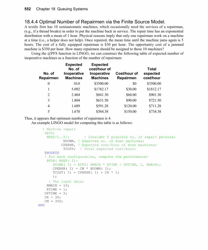
18.4.4 Optimal Number of Repairmen via the Finite Source Model. A textile firm has 10 semiautomatic machines, which occasionally need the services of a repairman,
(e.g., if a thread breaks) in order to put the machine back in service. The repair time has an exponential
distribution with a mean of 1 hour. Physical reasons imply that only one repairman work on a machine
at a time (i.e., a helper does not help). Once repaired, the mean time until the machine jams again is 5
hours. The cost of a fully equipped repairman is $30 per hour. The opportunity cost of a jammed
machine is $350 per hour. How many repairmen should be assigned to these 10 machines?
Using the @PFS function in LINGO, we can construct the following table of expected number of
inoperative machines as a function of the number of repairmen:
No. of Repairmen
Expected No. of
Inoperative Machines
Expected cost/hour of Inoperative Machines
Cost/hour of Repairmen
Total
expected cost/hour
0 10.0 $3500.00 $0 $3500.00
1 5.092 $1782.17 $30.00 $1812.17
2 2.404 $841.30 $60.00 $901.30
3 1.804 $631.50 $90.00 $721.50
4 1.689 $591.28 $120.00 $711.28
5 1.670 $584.38 $150.00 $734.38
Thus, it appears that optimum number of repairmen is 4.
An example LINGO model for computing this table is as follows:
! Machine repair
SETS:
NREP/1..5/: ! Consider 5 possible no. of repair persons;
NDOWN, ! Expected no. of down machines;
CPERHR, ! Expected cost/hour of down machines;
TCOST; ! Total expected cost/hour;
ENDSETS
! For each configuration, compute the performance-
@FOR( NREP( I):
NDOWN( I) = @PFS( NMACH * RTIME / UPTIME, I, NMACH);
CPERHR( I) = CM * NDOWN( I);
TCOST( I) = CPERHR( I) + CR * I;
);
! The input data;
NMACH = 10;
RTIME = 1;
UPTIME = 5;
CR = 30;
CM = 350;
END

Queuing Systems Chapter 18 553
Part of the solution is:
Variable Value
TCOST( 1) 1812.173
TCOST( 2) 901.3025
TCOST( 3) 721.5043
TCOST( 4) 711.2829
TCOST( 5) 734.3842
A model similar to the machine repairman has been used by Samuelson (1999) to analyze
predictive dialing methods in an outbound call center. In a predictive dialing system, an automatic
dialer may start dialing the next client to be contacted even before there is an agent available to talk to
the client. It takes anywhere from 10 to 30 seconds to dial a number and have the person dialed answer
the phone. So, the automatic dialing is done in the anticipation that an agent will become available by
the time that a called party answers the phone. An automatic dialer can detect a busy signal or a call
that is not answered, and can move on to dial the next number. Samuelson (1999) indicates that a good
predictive dialer can increase the agent talk time (i.e., utilization) to 95% from less than 80%. The
manager of a predictive dialer has at least two decision variables in controlling the predictive dialer:
a) how many additional lines to use, beyond the number of agents, for dialing, and b) the delay time
before starting dialing on a line once it becomes available. These two decisions can be fit into the
machine repairman as follows. The number of agents equals the number of repairmen. The number of
lines total is the population size. The up time is the delay time before initiating dialing + the dialing
time + time to answer.
18.4.5 Selection of a Processor Type via the M/G/1 Model You are about to install an ATM (Automated Teller Machine) at a new location. You have a choice
between two machines. The type A is a highly automated machine with a mean time to process a
transaction of 3 minutes with a standard deviation of 4.5 minutes. The type M machine is less
automated. It has a mean processing time of 4 minutes with a standard deviation of 1 minute. The
expected arrival rate is 10 customers/hour at the location in question. Which machine has a lower
expected waiting time? Which machine has a lower expected time in system?
There is a simple expression for the expected waiting time in a system with a single server for
which arrivals occur in a Poisson fashion and service times have a general distribution. If:
R = mean arrival rate,
T = mean service time,
SD = the standard deviation in service times, and
EW = expected waiting time,
then:
EW = R*( T*T + SD*SD)/[2*(1- R*T)].

554 Chapter 18 Queuing Systems
The following LINGO model illustrates:
! Single server queue with Poisson(Markovian) arrivals
and General service distribution, so-called M/G/1 queue;
DATA:
R = .1666667; ! Arrival rate in minutes(10/hour);
T = 3; ! Mean service time in minutes;
SD = 4.5; ! Standard deviation in service time;
ENDDATA
! Compute load( = Prob{ wait > 0});
RHO = R*T;
! Expected waiting time;
EW = R*( SD * SD + T * T)/(2*(1-RHO));
! Expected time in system;
ET = EW + T;
! Expected number waiting;
EN = R * EW;
! Expected number in system;
ES = R * ET;
The solution is:
Variable Value
R 0.1666667
T 3.000000
SD 4.500000
RHO 0.5000001
EW 4.875002
ET 7.875002
EN 0.8125005
ES 1.312501
To evaluate the slower, but less variable server, we change the data section to:
DATA:
R = .1666667; ! Arrival rate in minutes(10/hour);
T = 4; ! Mean service time in minutes;
SD = 1; ! Standard deviation in service time;
ENDDATA
Now, the solution is:
Variable Value
R 0.1666667
T 4.000000
SD 1.000000
RHO 0.6666668
EW 4.250003
ET 8.250003
EN 0.7083339
ES 1.375001
This is interesting. Due to the lower variability of the second server, the expected wait time is
lower with it. The first server, however, because it is faster, has a lower total time in system, ET. There
are some situations in which customers would prefer the longer expected time in system if it results in

Queuing Systems Chapter 18 555
a lower expected waiting time. One such setting might be a good restaurant. A typical patron would
like a low expected wait time, but might actually prefer a long leisurely service.
18.4.6 Multiple Server Systems with General Distribution, M/G/c & G/G/c There is no simple, “closed form” solution for a system with multiple servers, a service time
distribution that is non-exponential, and positive queue space. Whitt (1993), however, gives a simple
approximation. He gives evidence that the approximation is usefully accurate. Define:
SCVA = squared coefficient of variation of the interarrival time distribution
= (variance in interarrival times)/ (mean interarrival time squared)
= (variance in interarrival times)*R*R,
SCVT = squared coefficient of variation of the service time distribution
= (variance in service times)/(mean service time squared)
= (variance in service times/( T*T).
EWM(R,T,S) = expected waiting time in an M/M/c system with arrival rate R,
expected service time T, and S servers.
The approximation for the expected waiting time is then:
EWG(R,T,S,SCVA, SCVT)
= EWM(R,T,S)*(SCVA + SCVT)/2.
Note that for the exponential distribution, the coefficient of variation is one. It is fairly easy to
show that this approximation is in fact exact for M/G/1, M/M/c, M/G/, and when the system becomes
heavily loaded.

556 Chapter 18 Queuing Systems
Example
Suppose arrivals occur in a Poisson fashion at the rate of 50/hour (i.e., .8333333 per minute), there are
three servers, and the service time for each customer is exactly three minutes. A constant service time
implies that the service time squared coefficient of variation (SCVT) equals 0. Poisson arrivals implies
that the squared coefficient of variation of interarrival times (SCVA) equals 1. The model is:
! Compute approximate statistics for a (QGGC)
multi-server system with general arrivals,
and general service time distribution;
DATA:
R = .8333333; ! Mean arrival rate;
T = 3; ! Mean service time;
S = 3; ! Number of servers;
SCVA = 1; ! Squared coefficient of variation
of interarrival times;
SCVT = 0; ! Squared coefficient of variation
of service times;
ENDDATA
! The model;
! Average no. of busy servers;
LOAD = R * T;
! Probability a given call must wait;
PWAIT = @PEB( LOAD, S);
! Conditional expected wait, i.e., given must wait;
WAITCND = T/( S - LOAD);
! Unconditional expected wait;
WAITUNC = PWAIT * WAITCND;
! Unconditional approximate expected wait for
general distribution;
WAITG = WAITUNC * (SCVA + SCVT)/2;
The solution is:
Variable Value
R 0.8333333
T 3.000000
S 3.000000
SCVA 1.000000
SCVT 0.0000000
LOAD 2.500000
PWAIT 0.7022471
WAITCND 5.999999
WAITUNC 4.213482
WAITG 2.106741
Thus, the approximate expected wait time is about 2.1067. Later we will show that the expected
wait time can in fact be calculated exactly as 2.15. So, the approximation is not bad.

Queuing Systems Chapter 18 557
18.5 Critical Assumptions and Their Validity The critical assumptions implicit in the models discussed can be classified into three categories:
1) Steady state or stationarity assumptions.
2) Poisson arrivals assumption.
3) Service time assumptions.
The steady state assumption is that the system is not changing systematically over time (e.g., the
arrival rate is not changing over time in a cyclical fashion). Further, we are interested in performance
only after the system has been operating sufficiently long, so that the starting state has little effect on
the long run average. No real system strictly satisfies the steady state assumption. All systems start up
at some instant and terminate after some finite time. Arrival rates fluctuate in a predictable way over the
course of a day, week, month, etc. Nevertheless, the models discussed seemed to fit reality quite well in
many situations in spite of the lack of true stationarity in the real world. A very rough rule of thumb is that
if the system processing capacity is b customers/minute and the arrival rate is c customers/minute, then the
steady state formulae apply approximately after 1/(b - c) minutes. This corresponds roughly to one "busy
period."
The models discussed have assumed that service times are either constant or exponential
distributed. Performance tends to be relatively insensitive to the service time distribution (though still
dependent upon the mean service time) if either the system is lightly loaded or the available waiting
space is very limited. In fact, if there is no waiting space, then to compute the distribution of number in
system the only information needed about the service time distribution is its mean.
18.6 Networks of Queues Many systems, ranging from an office that does paperwork to a manufacturing plant, can be thought of
as a network of queues. As a job progresses through the system, it successively visits various service
or processing centers. The main additional piece of information one needs in order to analyze such a
system is the routing transition matrix, that is, a matrix of the form:
P(i,j) = Prob{ a job next visits processing center j | given that it just finished at center i}.
Jackson (1963) proved a remarkable result, essentially that if service times have an exponential
distribution and arrivals from the outside arrive according to a Poisson process, then each of the
individual queues in a network of queues can be analyzed by itself. The major additional piece of
information that one needs to analyze a given work center or station is the arrival rate to the station. If
we define REXT(j) = arrival rate to station j from the outside (or external) world, and R(j) = the arrival
rate at station j both from inside and outside, then it is fairly easy to show and also intuitive that the
R(j) should satisfy:
R(j) = REXT(j) + i R(i)* P(i,j).

558 Chapter 18 Queuing Systems
The following LINGO model illustrates how to solve this set of equations and then solve the
queuing problem at each station:
! Jackson queuing network model(qjacknet);
SETS:
CENTER: S, T, REXT, R, NQ, LOAD;
CXC( CENTER, CENTER): P;
ENDSETS
DATA:
! Get center name, number of servers,
mean service time and external arrival rate;
CENTER, S, T, REXT =
C1 2 .1 4
C2 1 .1 1
C3 1 .1 3;
! P(i,j) = Prob{ job next goes to i| given just
finished at j};
P = 0 .6 .4
.1 0 .4
.3 .3 0;
ENDDATA
! Solve for total arrival rate at each center;
@FOR( CENTER( I):
R( I) = REXT( I) + @SUM( CENTER( J): R( J) * P( I, J));
);
! Now solve the queuing problem at each center;
@FOR( CENTER( I):
! LOAD( I) = load on center I;
LOAD( I) = R( I) * T( I);
! Expected number at I = expected number waiting
+ expected number in service;
NQ(I) = ( LOAD( I)/( S( I) - LOAD( I)))
*@PEB( LOAD( I), S( I)) + LOAD( I);
! @PEB() = Prob{ all servers are busy at I};
);
! Expected time in system over all customers;
WTOT = @SUM( CENTER: NQ)/@SUM( CENTER: REXT);
Part of the solution is:
Variable Value
WTOT 0.6666667
R( C1) 10.00000
R( C2) 5.000000
R( C3) 7.500000
NQ( C1) 1.333333
NQ( C2) 1.000000
NQ( C3) 3.000000
LOAD( C1) 1.000000
LOAD( C2) 0.5000000
LOAD( C3) 0.7500000

Queuing Systems Chapter 18 559
18.7 Designer Queues In preceding sections, we gave some “canned” queuing models for the most common waiting line
situations. In this section, we present details on the calculations behind the queuing models. Thus, if
you want to design your own queuing system that does not quite match any of the standard situations,
you may be able to model your situation using the methods here.
18.7.1 Example: Positive but Finite Waiting Space System A common mode of operation for an inbound call center is to have, say 20 agents, but say, 30 phone
lines. Thus, a caller who finds a free phone line but all 20 agents busy, will be able to listen to soothing
music while waiting for an agent. A caller who finds 30 callers in the system will get a busy signal and
will have to give up.
First, define some general parameters:
r = arrival rate parameter. For the infinite source case, 1/r = mean time between
successive arrivals. For the finite source case, 1/r = mean time from when a given
customer finishes a service until it next requires service again (i.e., 1/r = mean up
time),
T = mean service time,
S = number of servers,
M = number of servers plus number of available waiting spaces.
We want to determine:
Pk = Prob {number customers waiting and being served = k}
If there are S servers, and M total lines or spaces, then the distribution of the number in system,
the Pk , satisfy the set of equations:
Pk = (rT/k)Pk-1 for k = 1, 2, ..., S
= (rT/S)Pk-1 for k = S + 1, S + 2, ..., M
and
P0 + P1 + ... + PM = 1.

560 Chapter 18 Queuing Systems
Here is a model that solves the above set of equations:
! M/M/c queue with limited space (qmmcf);
DATA:
! Number of servers;
S = 9;
! Total number of spaces;
M = 12;
! Arrival rate;
R = 4;
! Mean service time;
T = 2;
ENDDATA
SETS:
STATE/1..500/: P;
ENDSETS
! The basic equation for a Markovian(i.e., the time
til next transition has an exponential distribution) system,
says:(expected transitions into state k per unit time)
= (expected transitions out of state k per unit time);
! For state 1( P0 = prob{system is empty});
P0* R + P( 2)*2/T = ( R + 1/T) * P( 1);
! Remaining states with idle servers;
@FOR( STATE( K) | K #GT# 1 #AND# K #LT# S:
P( K - 1)* R + P( K+1)*(K+1)/T = ( R + K/T) * P( K)
);
! States with all servers busy;
@FOR( STATE( K) | K #GE# S #AND# K #LT# M:
P( K - 1)* R + P( K+1)*S/T = ( R + S/T) * P( K)
);
! All-full state is special;
P( M - 1)* R = (S/T)* P( M);
! The P(k)'s are probabilities;
P0 + @SUM( STATE( K)| K #LE# M: P( K)) = 1;
! Compute summary performance measures;
! Fraction lost;
FLOST = P( M);
! Expected number in system;
EN = @SUM( STATE( K)| K #LE# M: K * P( K));
! Expected time in system for those who enter;
ET = EN/( R *(1-FLOST));
! Expected wait time for those who enter;
EW = ET - T;

Queuing Systems Chapter 18 561
The solution is:
Variable Value
N 9.000000
M 12.00000
R 4.000000
T 2.000000
P0 0.3314540E-03
FLOST 0.8610186E-01
EN 7.872193
ET 2.153466
EW 0.153466
P( 1) 0.2651632E-02
P( 2) 0.1060653E-01
P( 3) 0.2828407E-01
P( 4) 0.5656815E-01
P( 5) 0.9050903E-01
P( 6) 0.1206787
P( 7) 0.1379185
P( 8) 0.1379185
P( 9) 0.1225942
P( 10) 0.1089727
P( 11) 0.9686459E-01
P( 12) 0.8610186E-01
This model has three extra waiting spaces or lines beyond the nine servers. The fraction demand
lost is 0.08610186. By comparison, if there were no extra lines, the fraction lost would be more than
twice as much, 0.1731408.
The above model is an example of balking. A prospective customer is said to balk if the customer
decides to not join the queue because the queue is too long. It is a common problem in systems where
the queue is visible (e.g., automotive fuel filling stations). More generalized forms of balking can be
modeled using methods of this chapter. One such form might be that an arriving customer balks with a
probability that is increasing in the length of the queue.
A phenomenon similar to balking is reneging. A customer in the waiting queue is said to renege if
she departs the waiting queue before having received service. For example, at internet websites it is not
uncommon for more than 50% of customers to abandon their “shopping carts” before getting to the
checkout step. Again, reneging behavior can be easily modeled using the methods of this section by
having a reneging rate that is, say proportional to the number waiting.
562 Chapter 18 Queuing Systems
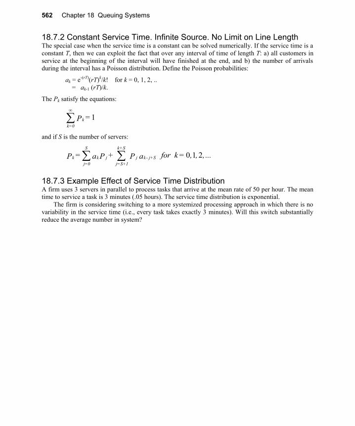
18.7.2 Constant Service Time. Infinite Source. No Limit on Line Length The special case when the service time is a constant can be solved numerically. If the service time is a
constant T, then we can exploit the fact that over any interval of time of length T: a) all customers in
service at the beginning of the interval will have finished at the end, and b) the number of arrivals
during the interval has a Poisson distribution. Define the Poisson probabilities:
ak = e-(rT)
(rT)k/k! for k = 0, 1, 2, ..
= ak-1 (rT)/k.
The Pk satisfy the equations:
1k
k=0
= P
and if S is the number of servers:
0 1 2S k+S
k j jk k- j+S
j=0 j=S+1
= + for k = , , , ...a aP P P
18.7.3 Example Effect of Service Time Distribution A firm uses 3 servers in parallel to process tasks that arrive at the mean rate of 50 per hour. The mean
time to service a task is 3 minutes (.05 hours). The service time distribution is exponential.
The firm is considering switching to a more systemized processing approach in which there is no
variability in the service time (i.e., every task takes exactly 3 minutes). Will this switch substantially
reduce the average number in system?
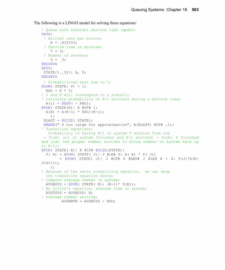
Queuing Systems Chapter 18 563
The following is a LINGO model for solving these equations:
! Queue with constant service time (qmdc);
DATA:
! Arrival rate per minute;
R = .833333;
! Service time in minutes;
T = 3;
! Number of servers;
S = 3;
ENDDATA
SETS:
STATE/1..35/: A, P;
ENDSETS
! Probabilities must sum to 1;
@SUM( STATE: P) = 1;
RHO = R * T;
! J and K will correspond to a state-1;
! Calculate probability of K-1 arrivals during a service time;
A(1) = @EXP( - RHO);
@FOR( STATE(K)| K #GT# 1:
A(K) = A(K-1) * RHO/(K-1);
);
NLAST = @SIZE( STATE);
@WARN(" S too large for approximation", A(NLAST) #GT# .1);
! Transition equations:
Probability of having K-1 in system T minutes from now
= Prob{ all in system finished and K-1 arrived} + Prob{ S finished
and just the proper number arrived to bring number in system back up
to K-1};
@FOR( STATE( K)| K #LT# @SIZE(STATE):
P( K) = @SUM( STATE( J)| J #LE# S: A( K) * P( J))
+ @SUM( STATE( J)| J #GT# S #AND# J #LE# K + S: P(J)*A(K-
J+S+1));
);
! Because of the extra normalizing equation, we can drop
one transition equation above;
! Compute average number in system;
AVGNSYS = @SUM( STATE( K): (K-1)* P(K));
! By Little's equation, average time in system;
AVGTSYS = AVGNSYS/ R;
! Average number waiting;
AVGNWTN = AVGNSYS - RHO;

564 Chapter 18 Queuing Systems
Part of the solution is:
Variable Value
RHO 2.499999
NLAST 35.00000
AVGNSYS 4.291565
AVGTSYS 5.149880
AVGNWTN 1.791566
P( 1) 0.3936355E-01
P( 2) 0.1102164
P( 3) 0.1615349
P( 4) 0.1684308
P( 5) 0.1438250
P( 6) 0.1097549
P( 7) 0.7924944E-01
P( 8) 0.5598532E-01
P( 9) 0.3930554E-01
P( 10) 0.2757040E-01
P( 11) 0.1934223E-01
P( 12) 0.1357152E-01
P( 13) 0.9522611E-02
It is of interest to compare this result with the case of exponentially distributed service times:
Exponential Service Distribution
Constant
Average No. in System 6.01 4.29
Average No. Waiting 3.51 1.79
Thus, there is a noticeable improvement associated with reducing the variability in service time. In
fact, in a heavily loaded system, reducing the variability as above will reduce the expected waiting
time by a factor of almost 2.

Queuing Systems Chapter 18 565
18.8 Problems 1. The Jefferson Mint is a Philadelphia based company that sells various kinds of candy by mail. It
has recently acquired the Toute-de-Suite Candy Company of New Orleans and the Amber
Dextrose Candy Company of Cleveland. The telephone has been an important source of orders for
all three firms. In fact, during the busiest three hours of the day (1 pm to 4 pm), Jefferson has been
taking calls at the rate of .98 per minute, Toute-de-Suite at the rate of .65 calls per minute, and
Dextrose at the rate of .79 calls per minute. All three find that on average it takes about three
minutes to process a call.
Jefferson would like to examine the wisdom of combining one or more of the three phone
order taking centers into a single order taking center in Philadelphia. This would require a phone
line from New Orleans to Philadelphia at a cost of $170 per day and/or a phone line from
Cleveland to Philadelphia at a cost of $140 per day. A phone order taker costs $75 per day.
Regardless of the configuration chosen, the desired service level is 95%. That is, at least 95% of
the calls should be answered immediately, else it is considered lost. This requirement is applicable
to the busiest time of the day in particular. This is considered reasonable for the kind of
semi-impulse buying involved. Note that only one phone line is needed to connect two cities. This
dedicated line can handle several dozen conversations simultaneously.
a) The New Orleans office could be converted first. What are the expected savings per day
of combining it with the Philadelphia office?
b) What is your complete recommendation?
c) The Cleveland office has been operating with four order takers. How might you wish to
question and possibly adjust the Cleveland call data?
2. Reliability is very important to a communications firm. The Exocom firm has a number of its
large digital communication switches installed around the country. It is concerned with how many
spares it should keep in inventory to quickly replace failed switches in the field. It estimates that
failures will occur in the field at the rate of about 1.5 per month. It is unattractive to keep a lot of
spares because the cost of each switch is $800,000. On the other hand, it is estimated that, if a
customer is without his switch, the cost is approximately $8,000 for each day out, including
weekends. This cost is borne largely by Exocom in the form of penalties and lost good will. Even
though a faulty switch can be replaced in about one hour, (once the replacement switch is on site),
it takes about one half month to diagnose and repair a faulty switch. Once repaired, a switch joins
the spares to hold. Exocom is anxious to get your advice because, if no more money need be
invested in spares, then there are about four other investment projects waiting in the wings, which
pass the company's 1.5% per month cost of capital threshold. What is your recommendation?

566 Chapter 18 Queuing Systems
3. Below is a record of long-distance phone calls made from one phone over an interval of time.
DESTINATION NUMBER DESTINATION NUMBER
DATE CITY STATE MINUTES DATE CITY STATE MINUTES
03/04 MICHIGANCY IN 0.4 03/21 NEW YORK NY 12.6
03/07 PHILA PA 3.1 03/21 PRINCETON NJ 2.0
03/07 LAFAYETTE IN 3.9 03/21 PRINCETON NJ 0.2
03/07 OSSINING NY 1.4 03/21 PRINCETON NJ 0.3
03/07 LAFAYETTE IN 2.8 03/21 PRINCETON NJ 0.3
03/08 LAFAYETTE IN 2.8 03/25 SANTA CRUZ CA 1.4
03/08 SOSAN FRAN CA 2.0 03/25 FORT WAYNE IN 0.9
03/08 PHILA PA 0.9 03/27 SANTA CRUZ CA 0.9
03/11 BOSTON MA 5.1 03/27 SANTA CRUZ CA 8.1
03/11 NEW YORK NY 3.1 03/27 SOSAN FRAN CA 8.2
03/15 MADISON WI 0.3 03/27 CHARLOTSVL VA 0.7
03/19 PHILA PA 3.6 03/28 CHARLOTSVL VA 8.4
03/20 PALO ALTO CA 4.7 03/28 NEW YORK NY 0.8
03/20 PALO ALTO CA 9.2 03/29 NEW YORK NY 1.7
DESTINATION NUMBER DESTINATION NUMBER
DATE CITY STATE MINUTES DATE CITY STATE MINUTES
03/29 BOSTON MA 0.6 04/16 CAMBRIDGE MA 0.9
04/01 HOUSTON TX 1.1 04/18 ROCHESTER NY 1.3
04/01 BOSTON MA 10.6 04/19 PALO ALTO CA 16.1
04/01 BRYAN TX 1.4 04/22 ROCHESTER NY 1.7
04/01 PEORIA IL 1.0 04/23 CHARLSTON IL 0.7
04/02 SANTA CRUZ CA 5.5 04/24 CHARLSTON IL 6.4
04/03 HOUSTON TX 1.4 04/24 WLOSANGLS CA 3.0
04/03 PEORIA IL 2.3 04/24 NEW YORK NY 5.1
04/09 NEW YORK NY 1.1 04/24 FORT WAYNE IN 0.9
04/11 LOS ALTOS CA 5.5 04/24 PORTAGE IN 2.2
a) How well does a Poisson distribution (perhaps appropriately modified) describe the call
per day behavior?
b) How well does an exponential distribution describe the number of minutes per call?
c) In what year were the calls made?