174mm Top: 12.653mm Gutter: 16 - TPU
196
Transcript of 174mm Top: 12.653mm Gutter: 16 - TPU


Trim: 247mm × 174mm Top: 12.653mm Gutter: 16.871mmCUUK2531-FM CUUK2531/Rasmuson ISBN: 978 1 107 04969 7 November 13, 2013 18:34
Mathematical Modeling in Chemical Engineering
A solid introduction to mathematical modeling for a range of chemical engineeringapplications, covering model formulation, simplification, and validation. It explains howto describe a physical/chemical reality in mathematical language and how to select thetype and degree of sophistication for a model. Model reduction and approximate methodsare presented, including dimensional analysis, time constant analysis, and asymptoticmethods. An overview of solution methods for typical classes of models is given. As finalsteps in model building, parameter estimation and model validation and assessment arediscussed. The reader is given hands-on experience of formulating new models, reducingthe models, and validating the models.
The authors assume a knowledge of basic chemical engineering, in particular transportphenomena, as well as basic mathematics, statistics, and programming. The accompa-nying problems, tutorials, and projects include model formulation at different levels,analysis, parameter estimation, and numerical solution.
Anders Rasmuson is a Professor in Chemical Engineering at Chalmers University ofTechnology, Gothenburg, Sweden. He obtained his PhD in chemical engineering atthe Royal Institute of Technology, Stockholm, in 1978. His research has focused onmathematical modeling combined with experimental work in many areas of chemicalengineering, for example particulate processes, multiphase flows and transport phenom-ena, mixing, and separation processes.
Bengt Andersson is a Professor in Chemical Engineering at Chalmers University ofTechnology. He obtained his PhD in chemical engineering at Chalmers in 1977. Hisresearch has focused on experimental studies and modeling of mass and heat transferin various chemical reactors, ranging from automotive catalysis to three-phase flow inchemical reactors.
Louise Olsson is a Professor in Chemical Engineering at Chalmers University ofTechnology. She obtained her PhD in chemical engineering at Chalmers in 2002. Herresearch has focused on experiments and kinetic modeling of heterogeneous catalysis.
Ronnie Andersson is an Assistant professor in Chemical Engineering at ChalmersUniversity of Technology. He obtained his PhD at Chalmers in 2005, and from 2005until 2010 he worked as consultant at Epsilon HighTech as a specialist in computationalfluid dynamic simulations of combustion and multiphase flows. His research projectsinvolve physical modeling, fluid dynamic simulations, and experimental methods.

Trim: 247mm × 174mm Top: 12.653mm Gutter: 16.871mmCUUK2531-FM CUUK2531/Rasmuson ISBN: 978 1 107 04969 7 November 13, 2013 18:34
Trim: 247mm × 174mm Top: 12.653mm Gutter: 16.871mmCUUK2531-FM CUUK2531/Rasmuson ISBN: 978 1 107 04969 7 November 13, 2013 18:34
Mathematical Modeling inChemical Engineering
ANDERS RASMUSONChalmers University of Technology, Gothenberg
BENGT ANDERSSONChalmers University of Technology, Gothenberg
LOUISE OLSSONChalmers University of Technology, Gothenberg
RONNIE ANDERSSONChalmers University of Technology, Gothenberg

Trim: 247mm × 174mm Top: 12.653mm Gutter: 16.871mmCUUK2531-FM CUUK2531/Rasmuson ISBN: 978 1 107 04969 7 November 13, 2013 18:34
University Printing House, Cambridge CB2 8BS, United Kingdom
Published in the United States of America by Cambridge University Press, New York
Cambridge University Press is part of the University of Cambridge.
It furthers the University’s mission by disseminating knowledge in the pursuit ofeducation, learning and research at the highest international levels of excellence.
www.cambridge.orgInformation on this title: www.cambridge.org/9781107049697
C© Cambridge University Press 2014
This publication is in copyright. Subject to statutory exceptionand to the provisions of relevant collective licensing agreements,no reproduction of any part may take place without the writtenpermission of Cambridge University Press.
First published 2014
Printed in the United Kingdom by MPG Printgroup Ltd, Cambridge
A catalog record for this publication is available from the British Library
Library of Congress Cataloging in Publication data
ISBN 978-1-107-04969-7 Hardback
Cambridge University Press has no responsibility for the persistence or accuracy ofURLs for external or third-party internet websites referred to in this publication,and does not guarantee that any content on such websites is, or will remain,accurate or appropriate.

Trim: 247mm × 174mm Top: 12.653mm Gutter: 16.871mmCUUK2531-FM CUUK2531/Rasmuson ISBN: 978 1 107 04969 7 November 13, 2013 18:34
Contents
Preface page ix
1 Introduction 1
1.1 Why do mathematical modeling? 11.2 The modeling procedure 51.3 Questions 9
2 Classification 10
2.1 Grouping of models into opposite pairs 102.2 Classification based on mathematical complexity 142.3 Classification according to scale (degree of physical detail) 162.4 Questions 18
3 Model formulation 20
3.1 Balances and conservation principles 203.2 Transport phenomena models 223.3 Boundary conditions 263.4 Population balance models 28
3.4.1 Application to RTDs 323.5 Questions 343.6 Practice problems 35
4 Empirical model building 40
4.1 Dimensional systems 404.2 Dimensionless equations 414.3 Empirical models 464.4 Scaling up 484.5 Practice problems 52
5 Strategies for simplifying mathematical models 53
5.1 Reducing mathematical models 54

Trim: 247mm × 174mm Top: 12.653mm Gutter: 16.871mmCUUK2531-FM CUUK2531/Rasmuson ISBN: 978 1 107 04969 7 November 13, 2013 18:34
vi Contents
5.1.1 Decoupling equations 555.1.2 Reducing the number of independent variables 555.1.3 Lumping 565.1.4 Simplified geometry 565.1.5 Steady state or transient 585.1.6 Linearizing 615.1.7 Limiting cases 635.1.8 Neglecting terms 645.1.9 Changing the boundary conditions 67
5.2 Case study: Modeling flow, heat, and reaction in a tubular reactor 685.2.1 General equation for a cylindrical reactor 685.2.2 Reducing the number of independent variables 695.2.3 Steady state or transient? 705.2.4 Decoupling equations 725.2.5 Simplified geometry 725.2.6 Limiting cases 755.2.7 Conclusions 76
5.3 Error estimations 765.3.1 Sensitivity analysis 775.3.2 Over- and underestimations 77
5.4 Questions 775.5 Practice problems 78
6 Numerical methods 81
6.1 Ordinary differential equations 816.1.1 ODE classification 816.1.2 Solving initial-value problems 826.1.3 Numerical accuracy 876.1.4 Adaptive step size methods and error control 886.1.5 Implicit methods and stability 906.1.6 Multistep methods and predictor–corrector pairs 936.1.7 Systems of ODEs 946.1.8 Transforming higher-order ODEs 966.1.9 Stiffness of ODEs 97
6.2 Boundary-value problems 996.2.1 Shooting method 996.2.2 Finite difference method for BVPs 1026.2.3 Collocation and finite element methods 107
6.3 Partial differential equations 1086.3.1 Classification of PDEs 1096.3.2 Finite difference solution of parabolic equations 1106.3.3 Forward difference method 1106.3.4 Backward difference method 113

Trim: 247mm × 174mm Top: 12.653mm Gutter: 16.871mmCUUK2531-FM CUUK2531/Rasmuson ISBN: 978 1 107 04969 7 November 13, 2013 18:34
Contents vii
6.3.5 Crank–Nicolson method 1146.4 Simulation software 114
6.4.1 MATLAB 1146.4.2 Miscelleanus MATLAB algorithms 1156.4.3 An example of MATLAB code 1166.4.4 GNU Octave 117
6.5 Summary 1176.6 Questions 1176.7 Practice problems 118
7 Statistical analysis of mathematical models 121
7.1 Introduction 1217.2 Linear regression 121
7.2.1 Least square method 1237.3 Linear regression in its generalized form 125
7.3.1 Least square method 1267.4 Weighted least squares 127
7.4.1 Stabilization of the variance 1277.4.2 Placing greater/less weight on certain experimental parts 128
7.5 Confidence intervals and regions 1307.5.1 Confidence intervals 1307.5.2 Student’s t-tests of individual parameters 1337.5.3 Confidence regions and bands 134
7.6 Correlation between parameters 1367.6.1 Variance and co-variance 1367.6.2 Correlation matrix 137
7.7 Non-linear regression 1387.7.1 Intrinsically linear models 1387.7.2 Non-linear models 1397.7.3 Approximate confidence levels and regions for non-linear models 1407.7.4 Correlation between parameters for non-linear models 142
7.8 Model assessments 1427.8.1 Residual plots 1427.8.2 Analysis of variance (ANOVA) table 1457.8.3 R2 statistic 149
7.9 Case study 7.1: Statistical analysis of a linear model 1497.9.1 Solution 150
7.10 Case study 7.2: Multiple regression 1537.10.1 Solution 154
7.11 Case study 7.3: Non-linear model with one predictor 1587.11.1 Solution 159
7.12 Questions 1637.13 Practice problems 163

Trim: 247mm × 174mm Top: 12.653mm Gutter: 16.871mmCUUK2531-FM CUUK2531/Rasmuson ISBN: 978 1 107 04969 7 November 13, 2013 18:34
viii Contents
Appendix A Microscopic transport equations 168Appendix B Dimensionless variables 170Appendix C Student’s t-distribution 173
Bibliography 180Index 181

Trim: 247mm × 174mm Top: 12.653mm Gutter: 16.871mmCUUK2531-FM CUUK2531/Rasmuson ISBN: 978 1 107 04969 7 November 13, 2013 18:34
Preface
The aim of this textbook is to give the reader insight and skill in the formulation,construction, simplification, evaluation/interpretation, and use of mathematical modelsin chemical engineering. It is not a book about the solution of mathematical models,even though an overview of solution methods for typical classes of models isgiven.
Models of different types and complexities find more and more use in chemicalengineering, e.g. for the design, scale-up/down, optimization, and operation of reactors,separators, and heat exchangers. Mathematical models are also used in the planning andevaluation of experiments and for developing mechanistic understanding of complexsystems. Examples include balance models in differential or integral form, and algebraicmodels, such as equilibrium models.
The book includes model formulation, i.e. how to describe a physical/chemical realityin mathematical language, and how to choose the type and degree of sophistication ofa model. It is emphasized that this is an iterative procedure where models are graduallyrefined or rejected in confrontation with experiments. Model reduction and approximatemethods, such as dimensional analysis, time constant analysis, and asymptotic methods,are treated. An overview of solution methods for typical classes of models is given.Parameter estimation and model validation and assessment, as final steps, in modelbuilding are discussed. The question “What model should be used for a given situation?”is answered.
The book is accompanied by problems, tutorials, and projects. The projects, in smallerteams, include model formulation at different levels, analysis, parameter estimation, andnumerical solution.
The book is aimed at chemical engineering students, and a knowledge basic chemicalengineering, in particular transport phenomena, will be assumed. Basic mathematics,statistics, and programming skills are also required.
Using the book (course) the reader should be able to construct, solve, and applymathematical models for chemical engineering problems. In particular:
� construct models using balances on differential or macroscopic control volumes formomentum, heat, mass, and numbers (population balances);
� construct models by simplification of general model equations;

Trim: 247mm × 174mm Top: 12.653mm Gutter: 16.871mmCUUK2531-FM CUUK2531/Rasmuson ISBN: 978 1 107 04969 7 November 13, 2013 18:34
x Preface
� understand and use methods for model simplification;� understand differences between models;� understand and use numerical solution methods;� understand and perform parameter estimation;� use model assessment techniques to be able to judge if a model is good enough.

Trim: 247mm × 174mm Top: 12.653mm Gutter: 16.871mmCUUK2531-01 CUUK2531/Rasmuson ISBN: 978 1 107 04969 7 November 13, 2013 15:20
1 Introduction
In this introductory chapter the use of mathematical models in chemical engineering ismotivated and examples are given. The general modeling procedure is described, andsome important tools that are covered in greater detail later in the book are outlined.
1.1 Why do mathematical modeling?
Mathematical modeling has always been an important activity in science and engineering.The formulation of qualitative questions about an observed phenomenon as mathematicalproblems was the motivation for and an integral part of the development of mathematicsfrom the very beginning.
Although problem solving has been practised for a very long time, the use of math-ematics as a very effective tool in problem solving has gained prominence in the last50 years, mainly due to rapid developments in computing. Computational power is par-ticularly important in modeling chemical engineering systems, as the physical and chem-ical laws governing these processes are complex. Besides heat, mass, and momentumtransfer, these processes may also include chemical reactions, reaction heat, adsorption,desorption, phase transition, multiphase flow, etc. This makes modeling challenging butalso necessary to understand complex interactions.
All models are abstractions of real systems and processes. Nevertheless, they serveas tools for engineers and scientists to develop an understanding of important systemsand processes using mathematical equations. In a chemical engineering context, math-ematical modeling is a prerequisite for:
� design and scale-up;� process control;� optimization;� mechanistic understanding;� evaluation/planning of experiments;� trouble shooting and diagnostics;� determining quantities that cannot be measured directly;� simulation instead of costly experiments in the development lab;� feasibility studies to determine potential before building prototype equipment or
devices.

Trim: 247mm × 174mm Top: 12.653mm Gutter: 16.871mmCUUK2531-01 CUUK2531/Rasmuson ISBN: 978 1 107 04969 7 November 13, 2013 15:20
2 Introduction
Figure 1.1. Pilot dryer, Example 1.1.
A typical problem in chemical engineering concerns scale-up from laboratory to full-scale equipment. To be able to scale-up with some certainty, the fundamental mecha-nisms have to be evaluated and formulated in mathematical terms. This involves carefulexperimental work in close connection to the theoretical development.
There are no modeling recipes that guarantee successful results. However, the devel-opment of new models always requires both an understanding of the physical/chemicalprinciples controlling a process and the skills for making appropriate simplifyingassumptions. Models will never be anything other than simplified representations of realprocesses, but as long as the essential mechanisms are included the model predictions canbe accurate. Chapter 3 therefore provides information on how to formulate mathematicalmodels correctly and Chapter 4 teaches the reader how to simplify the models.
Let us now look at two examples and discuss the mechanisms that control thesesystems. We do this without going into the details of the formulation or numericalsolution. After reading this book, the reader is encouraged to refer back to these twocase studies and read how these modeling problems were solved.
Example 1.1 Design of a pneumatic conveying dryerA mathematical model of a pneumatic conveying dryer, Figure 1.1, has been developed(Fyhr, C. and Rasmuson; A., AIChE J. 42, 2491–2502, 1996; 43, 2889–2902, 1997)and validated against experimental results in a pilot dryer.

Trim: 247mm × 174mm Top: 12.653mm Gutter: 16.871mmCUUK2531-01 CUUK2531/Rasmuson ISBN: 978 1 107 04969 7 November 13, 2013 15:20
1.1 Why do mathematical modeling? 3
Figure 1.2. Interactions between particles, steam, and walls.
Figure 1.3. Wood chip.
The dryer essentially consists of a long tube in which the material is conveyed by, inour case, superheated steam. The aim of the modeling task was to develop a tool thatcould be used for design and rating purposes.
Inside the tubes, the single particles, conveying steam, and walls interact in a complexmanner, as illustrated in Figure 1.2.
The gas and particles exchange heat and mass due to drying, and momentum in orderto convey the particles. The gas and walls exchange momentum by wall friction, as wellas heat by convection. The single particles and walls also exchange momentum by wallfriction, and heat by radiation from the walls. The single particle is, in this case, a woodchip shaped as depicted in Figure 1.3.
The chip is rectangular, which leads to problems in determining exchange coefficients.The particles also flow in a disordered manner through the dryer. The drying rate iscontrolled by external heat transfer as long as the surface is kept wet. As the surfacedries out, the drying rate decreases and becomes a function of both the external andinternal characteristics of the drying medium and single particle. The insertion of coldmaterial into the dryer leads to the condensation of steam on the wood chip surface,which, initially, increases the moisture content of the wood chip. The pressure drop atthe outlet leads to flashing, which, in contrast, reduces the moisture content.
The mechanisms that occur between the particles and the steam, as well as themechanisms inside the wood chip, are thus complex, and a detailed understanding isnecessary.
How would you go about modeling this problem? Models for these complex processeshave been developed in the cited articles by Fyhr and Rasmusson.

Trim: 247mm × 174mm Top: 12.653mm Gutter: 16.871mmCUUK2531-01 CUUK2531/Rasmuson ISBN: 978 1 107 04969 7 November 13, 2013 15:20
4 Introduction
Figure 1.4. Schematic of a Wurster bed, Example 1.2.
Example 1.2 Design and optimization of a Wurster bed coaterIn the second example, a mathematical model of a Wurster bed coater, Figure 1.4, hasbeen developed (Karlsson, S., Rasmuson, A., van Wachen, B., and Niklasson Bjorn, I.,AIChE J. 55, 2578–2590, 2009; Karlsson, S., Rasmusson, A., Niklasson Bjorn, I., andSchantz, S., Powder Tech. 207, 245–256, 2011) and validated against experimentalresults. Coating is a common process step in the chemical, agricultural,pharmaceutical, and food industries. Coating of solid particles is used for the sustainedrelease of active components, for protection of the core from external conditions, formasking taste or odours, and for easier powder handling. For example, severalapplications in particular are used for coating in the pharmaceutical industry, for bothaesthetic and functional purposes.
The Wurster process is a type of spouted bed with a draft tube and fluidization flowaround the jet (Figure 1.4). The jet consists of a spray nozzle that injects air and droplets

Trim: 247mm × 174mm Top: 12.653mm Gutter: 16.871mmCUUK2531-01 CUUK2531/Rasmuson ISBN: 978 1 107 04969 7 November 13, 2013 15:20
1.2 The modeling procedure 5
of the coating liquid into the bed. The droplets hit and wet the particles cocurrentlyin the inlet to the draft tube. The particles are transported upwards through the tube,decelerate in the expansion chamber, and fall down to the dense region of particlesoutside the tube. During the upward movement and the deceleration, the particles aredried by the warm air, and a thin coating layer starts to form on the particle surface.From the dense region the particles are transported again into the Wurster tube, wherethe droplets again hit the particles, and the circulation motion in the bed is repeated.The particles are circulated until a sufficiently thick layer of coating material has beenbuilt up around them.
The final coating properties, such as film thickness distribution, depend not only onthe coating material, but also on the process equipment and the operating conditionsduring film formation. The spray rate, temperature, and moisture content are operatingparameters that influence the final coating and which can be controlled in the process.The drying rate and the subsequent film formation are highly dependent on the flow fieldof the gas and the particles in the equipment. Local temperatures in the equipment arealso known to be critical for the film formation; different temperatures may change theproperties of the coating layer. Temperature is also important for moisture equilibrium,and influences the drying rate.
Several processes take place simultaneously at the single-particle level during thecoating phase. These are: the atomization of the coating solution, transport of thedroplets formed to the particle, adhesion of the droplets to the particle surface, surfacewetting, and film formation and drying. These processes are repeated for each appliedfilm layer, i.e. continuously repeated for each circulation through the Wurster bed.
Consequently, the mechanisms that occur at the microscopic and macroscopic levelsare complex and include a high degree of interaction. The aim of the modeling task isto develop a tool that can be used for design and optimization.
What models do you think best describe the mechanisms in this process?
1.2 The modeling procedure
In undergraduate textbooks, models are often presented in their final, neat and elegantform. In reality there are many steps, choices, and iterative processes that a modeler goesthrough in reaching a satisfactory model. Each step in the modeling process requires anunderstanding of a variety of concepts and techniques blended with a combination ofcritical and creative thinking, intuition and foresight, and decision making. This makesmodel building both a science and an art.
Model building comprises different steps, as shown in Figure 1.5. As seen here,model develpoment is an iterative process of hypotheses formulation, validation, andrefinement.
Figure 1.5 also gives an outline of this process. Conceptual and mathematical modelformulation are treated further in Chapters 3–5; solution methods are discussed inChapter 6; and finally parameter estimation and model validation are discussed inChapter 7.

Trim: 247mm × 174mm Top: 12.653mm Gutter: 16.871mmCUUK2531-01 CUUK2531/Rasmuson ISBN: 978 1 107 04969 7 November 13, 2013 15:20
6 Introduction
Figure 1.5. The different steps in model development.
Step 1: Problem definitionThe first step in the mathematical model development is to define the problem. Thisinvolves stating clear goals for the modeling, including the various elements that pertainto the problem and its solution.
Consider the following questions:
What is the objective (i.e. what questions should the model be able to answer)?What resolution is needed?What degree of accuracy is required?
Step 2: Formulation of conceptual model (Chapter 3)When formulating the conceptual model, decisions must be made on what hypothesis andwhich assumptions to use. The first task is to collect data and experience about the subjectto be modeled. The main challenges are in identifying the underlying mechanisms andgoverning physical/chemical principles of the problem. The development of a conceptualmodel involves idealization, and there will always be a tradeoff between model generalityand precision.
Step 3: Formulation of mathematical model (Chapters 3–5)Each important quantity is represented by a suitable mathematical entity, e.g. a variable,a function, a graph, etc.
What are the variables (dependent, independent, parameters)?

Trim: 247mm × 174mm Top: 12.653mm Gutter: 16.871mmCUUK2531-01 CUUK2531/Rasmuson ISBN: 978 1 107 04969 7 November 13, 2013 15:20
1.2 The modeling procedure 7
The distinction between dependent and independent variables is that the independentvariable is the one being changed, x, and the dependent variable, y, is the observedvariable caused by this change, e.g. y = x3. Parameters represent physical quantitiesthat characterize the system and model such as density, thermal conductivity, viscosity,reaction rate constants, or activation energies. Parameters are not necessarily constants,and can be described as functions of the dependent (or independent) variables, e.g. heatcapacity cp(T) and density ρ(p,T).
What are the constraints? Are there limitations on the possible values of a variable.For example, concentrations are always positive.
What boundary conditions, i.e. the relations valid at the boundaries of the system aresuitable to use?
What initial conditions, i.e. conditions valid at the start-up of a time dependent process,exist?
Each relationship is represented by an equation, inequality, or other suitable mathe-matical relation.
Step 4: Solution of the mathematical problem (Chapter 6)Check the validity of individual mathematical relationships, and whether the relation-ships are mutually consistent.
Consider the analytical versus the numerical solution. Analytical solutions are onlypossible for special situations; essentially the problem has to be linear. Most often, anumerical solution is the only option; luckily the cost of computers is low and modelscan run in parallel on computer clusters if necessary.
Verify the mathematical solution, i.e. ensure that you have solved the equationscorrectly. This step involves checking your solution against previously known results(analytical/numerical), simplified limiting cases, etc.
Step 5: Estimation of parameters (Chapter 7)The parameters of the system must be evaluated and the appropriate values must beused in the model. Some parameters can be obtained independently of the mathematicalmodel. They may be of a basic character, like the gravitation constant, or it may bepossible to determine them by independent measurements, like, for instance, solubilitydata from solubility experiments. However, it is usually not possible to evaluate all theparameters from specific experiments, and many of them have to be estimated by takingresults from the whole (or a similar system), and then using parameter-fitting techniquesto determine which set of parameter values makes the model best fit the experimentalresults. For example, a complex reaction may involve ten or more kinetic constants.These constants can be estimated by fitting a model to results from a laboratory reactor.Once the parameter values have been determined, they can be incorporated into a modelof a plant-scale reactor.
Step 6: Evaluation/validation (Chapter 7)A key step in mathematical modeling is experimental validation. Ideally the validationshould be made using independent experimental results, i.e. not the same set as used

Trim: 247mm × 174mm Top: 12.653mm Gutter: 16.871mmCUUK2531-01 CUUK2531/Rasmuson ISBN: 978 1 107 04969 7 November 13, 2013 15:20
8 Introduction
for parameter estimation. During the validation procedure it may happen that the modelstill has some deficiencies. In that case, we have to “iterate” the model and eventuallymodify it. In recent work by Melander, O. and Rasmuson, A. (Nordic Pulp Paper Res.J. 20, 78–86, 2005) it was found that the original model for pulp fiber flow in a gasstream severely underestimated lateral spreading of the fibers. Detailed analysis led toa modified model (Melander, O. and Rasmuson, A., J. Multiphase Flow 33, 333–346,2007) with an additional term in the governing equations, and good agreement withexperimental data.
In Chapter 7, the general question of model quality is discussed. Is the model goodenough?
In the evaluation of the model, sensitivity analysis, i.e. the change in model outputdue to uncertainties in parameter values, is important.
There are certain characteristics that models have to varying degrees and which havea bearing on the question of how good they are:
� accuracy (is the output of the model correct?);� descriptive realism (i.e. based on correct assumptions);� precision (are predictions in the form of definite numbers?);� robustness (i.e. relatively immune to errors in the input data);� generality (applicable to a wide variety of situations);� fruitfulness (a model is considered fruitful if its conclusions are useful or if it inspires
development of other good models).
Step 7: Interpretation/applicationThe validated model is then ready to be used for one or several purposes as describedearlier, e.g. to enhance our understanding, make predictions, and give information abouthow to control the process.
Let us conclude this chapter with a classical modeling problem attributable to GalileoGalilei (1564–1642).
Example 1.3 Galileo´s gravitation modelsOne of the oldest scientific investigations was the attempt to understand gravity. Thisproblem provides a nice illustration of the steps in modeling.
“Understanding” gravity is too vague and ambitious a goal. A more specific questionabout gravity is:
Why do objects fall to the earth?
Aristotle´s answer was that objects fall to the earth because that is their natural place,but this never led to any useful science or mathematics. Around the time of Galileo(early seventeenth century), people began asking how gravity worked instead of why itworked. For example, Galileo wanted to describe the way objects gain velocity as theyfall. One particular question Galileo asked was:

Trim: 247mm × 174mm Top: 12.653mm Gutter: 16.871mmCUUK2531-01 CUUK2531/Rasmuson ISBN: 978 1 107 04969 7 November 13, 2013 15:20
1.3 Questions 9
What relation describes how a body gains velocity as it falls?
The next step is to identify relevant factors. Galileo decided to take into account onlydistance, time, and velocity. However, he might have also considered the weight, shape,and density of the object as well as air conditions.
The first assumption Galileo made was:
Assumption 1 If a body falls from rest, its velocity at any point is proportional to the distancealready fallen.
The mathematical description of Assumption 1 is:
dx
dt= ax . (1.1)
This equation has the solution
x = keat . (1.2)
The constant k is evaluated by
x(0) = 0, (1.3)
giving k = 0, and thus
x = 0 for all t.
The implication is that the object will never move, no matter how long we wait!Since this conclusion is clearly absurd, and there are no mistakes in the mathemat-
ical manipulation, the model has to be reformulated. Galileo eventually came to thisconclusion, and replaced Assumption 1 with:
Assumption 2 If a body falls from rest, its velocity at any point is proportional to the time it hasbeen falling.
The mathematical description of this assumption is:
dx
dt= bt, (1.4)
and the solution, with x(0) = 0, is
x = bt2. (1.5)
This law of falling bodies agrees well with observations in many circumstances, andthe parameter b can be estimated from matching experimental data. Incidentally, themodel constant b equals the gravitational constant, g.
1.3 Questions
(1) Give some reasons for doing mathematical modeling in chemical engineering.
(2) Explain why the model development often becomes an iterative procedure.

Trim: 247mm × 174mm Top: 12.653mm Gutter: 16.871mmCUUK2531-02 CUUK2531/Rasmuson ISBN: 978 1 107 04969 7 November 13, 2013 15:26
2 Classification
In this chapter mathematical models are classified by
� grouping into opposite pairs;� mathematical complexity;� degree of resolution.
The intention is to give the reader an understanding of differences between models asreflected by the modeling goal. Which question is the model intended to answer?
2.1 Grouping of models into opposite pairs
In this section, we will examine various types of mathematical models. There are manypossible ways of classification. One possibility is to group the models into oppositepairs:
� linear versus nonlinear;� steady state versus non-steady state;� lumped parameter versus distributed parameter;� continuous versus discrete variables;� deterministic versus stochastic;� interpolation versus extrapolation;� mechanistic versus empirical;� coupled versus not coupled.
Linear versus nonlinearLinear models exhibit the important property of superposition; nonlinear ones do not.Equations (and thus models) are linear if the dependent variables or their derivativesappear only to the first power; otherwise they are nonlinear. In practice, the ability touse a linear model for a process is of great significance. General analytical methodsfor equation solving are all based on linearity. Only special classes of nonlinear modelscan be attacked with mathematical methods. For the general case, where a numericalmethod is required, the amount of computation is also much less for linear models, andin addition error estimates and convergence criteria are usually derived under linearassumptions.

Trim: 247mm × 174mm Top: 12.653mm Gutter: 16.871mmCUUK2531-02 CUUK2531/Rasmuson ISBN: 978 1 107 04969 7 November 13, 2013 15:26
2.1 Grouping of models into opposite pairs 11
Steady state versus transientOther synonyms for steady state are time invariant, static, or stationary. These termsrefer to a process in which the point values of the dependent variables remain constantover time, as at steady state and at equilibrium. Non-steady-state processes are alsocalled unsteady state, transient, or dynamic, and represent a situation in which theprocess dependent variables change with respect to time. A typical example of annon-steady-state process is the startup of a distillation column which would eventuallyreach a pseudosteady-state set of operating conditions. Inherently transient processesinclude fixed-bed adsorption, batch distillation, and reactors, drying, and filtration/sedimentation.
Lumped parameter versus distributed parameterA lumped-parameter representation means that spatial variations are ignored, and thevarious properties and the state of a system can be considered homogeneous throughoutthe entire volume. A distributed-parameter representation, in contrast, takes into accountdetailed variations in behavior from point to point throughout the system. All real systemsare, of course, distributed in that there some variations occur throughout them. As thevariations are often relatively small, they may be ignored, and the system may then be“lumped.”
The answer to the question whether or not lumping is valid for a process modelis far from simple. A good rule of thumb is that if the response of the process is“instantaneous” throughout the process, then the process can be lumped. If the responseshows instantaneous differences throughout the process (or vessel), then it should notbe lumped. Note that the purpose of the model affects its validity. Had the purposebeen, for example, to study mixing in a stirred tank reactor, a lumped model would becompletely unsuitable because it has assumed from the first that the mixing is perfectand the concentration a single variable.
Because the mathematical procedures for solving lumped-parameter models are sim-pler than those for solving distributed-parameter models, we often approximate thelatter using an equivalent lumped-parameter system. Whilst lumping is often possible,we must be careful to avoid masking the salient features of a distributed element andsubsequently building an inadequate model by lumping.
As an example of the use of lumped versus distributed mathematical models, considerthe equilibrium stage concept of distillation, extraction, and similar processes. As shownin Figure 2.1, we usually assume that the entire stage acts as a whole, and we do notconsider variations in temperature, composition, or pressure in various parts of thestage. All of these variables are “lumped” together into some overall average. The errorsintroduced are compensated for by the stage efficiency factor.
Continuous versus discrete variablesContinuous means that the variables can assume any values within an interval; discretemeans that a variable can take on only distinct values within an interval. For example,concentrations in a countercurrent packed bed are usually modeled in terms of continuousvariables, whereas plate absorbers are modeled in terms of staged multicompartment

Trim: 247mm × 174mm Top: 12.653mm Gutter: 16.871mmCUUK2531-02 CUUK2531/Rasmuson ISBN: 978 1 107 04969 7 November 13, 2013 15:26
12 Classification
Figure 2.1. Lumped-parameter and distributed-parameter visualization of a distillation tray.(a) Actual plate with complex flow patterns and resulting variations in properties from point topoint. (b) Idealized equilibrium stage ignoring all internal variations.
Figure 2.2. Continuous versus discrete modeling of a packed column absorber.
models in which a concentration is uniform at each stage but differs from stage to stage indiscrete jumps. Continuous models are described by differential equations and discretemodels by difference equations. Figure 2.2 illustrates the two configurations.
The left-hand figure shows a packed column modeled as a continuous system, whereasthe right-hand figure represents the column as a sequence of discrete (staged) units. Theconcentrations in the left-hand column would be continuous variables; those in the right-hand column would involve discontinuous jumps. The tic marks in the left-hand columnrepresent hypothetical stages for analysis. It is, of course, possible to model the packed

Trim: 247mm × 174mm Top: 12.653mm Gutter: 16.871mmCUUK2531-02 CUUK2531/Rasmuson ISBN: 978 1 107 04969 7 November 13, 2013 15:26
2.1 Grouping of models into opposite pairs 13
Figure 2.3. Danger of extrapolation. Yield of a chemical reactor versus time.
column in terms of imaginary segregated stages and to treat the plate column in termsof partial differential equations in which the concentrations are continuous variables.
Deterministic versus stochasticDeterministic models or elements of models are those in which each variable andparameter can be assigned a definite fixed number, or a series of numbers, for any givenset of conditions, i.e. the model has no components that are inherently uncertain. Incontrast, the principle of uncertainty is introduced in stochastic or probabilistic models.The variables or parameters used to describe the input–output relationships and thestructure of the elements (and the constraints) are not precisely known. A stochasticmodel involves parameters characterized by probability distributions. Due to this thestochastic model will produce different results in each realization.
Stochastic models play an important role in understanding chaotic phenomena such asBrownian motion and turbulence. They are also used to describe highly heterogeneoussystems, e.g. transport in fractured media. Stochastic models are used in control theoryto account for the irregular nature of disturbances.
In the present context, we will focus upon deterministic models.
Interpolation versus extrapolationA model based on interpolation implies that the model is fitted to experimentally deter-mined values at different points and that the model is used to interpolate betweenthese points. A model used for extrapolation, in comparison, goes beyond the range ofexperimental data.
Typically, thermodynamic models are used for interpolation as well as correlationsin complicated transport phenomena applications. Extrapolation requires, in general, adetailed mechanistic understanding of the system. The procedure requires great care toavoid misleading conclusions. Figure 2.3 illustrates an exaggerated case of extrapolation

Trim: 247mm × 174mm Top: 12.653mm Gutter: 16.871mmCUUK2531-02 CUUK2531/Rasmuson ISBN: 978 1 107 04969 7 November 13, 2013 15:26
14 Classification
by means of a linear model into a region beyond the range of experimental data for achemical reaction that reaches a maximum yield in time.
In the safety analysis of nuclear waste repositories models are used to predict the fate ofleaking radionuclides into the surrounding rock formation over geological time scales.Naturally, it is of the utmost importance that these models are physically/chemicallysound and based on well-understood mechanistic principles.
Mechanistic versus empiricalMechanistic means that models are based on the underlying physics and chemistrygoverning the behavior of a process; empirical means that models are based on correlatedexperimental data. Empirical modeling depends on the availability of process data,whereas mechanistic modeling does not; however, a fundamental understanding of thephysics and chemistry of the process is required. Mechanistic models are preferablyused in process design, whereas empirical models can be used when only trends areneeded, such as in process control. Semi-empirical models cover the range in between.This discussion closely resembles the one regarding extrapolation/interpolation.
Coupled versus not coupledWhen a model consists of two or more interacting relations, we have a coupled model.The coupling may be weak or strong. If the interaction only works in one direction, wespeak of weak coupling (one-way coupling); if it operates in both directions we speak ofstrong (two-way) coupling. Forced convection is an example of one-way coupling, andfree convection is an example of two-way coupling. In forced convection, the flow fieldis independent of the transport of energy and can be solved first and then introducedinto the energy equation. In free convection, flow and energy transport are intimatelycoupled since the flow is generated by density differences originating from temperaturedifferences. A model of a pneumatic conveying dryer involves a high degree of coupling(see Example 1.1).
2.2 Classification based on mathematical complexity
Another classification scheme to be considered is shown in Figure 2.4.It can be seen that the complexity of solving a mathematical problem roughly increases
as we go down Figure 2.4. In other words, algebraic equations are usually easier tosolve than ordinary differential equations, which in turn are usually easier to solvethan partial differential equations. This is not always true, of course, since a linearpartial differential equation may be easier to solve than a non-linear ordinary differentialequation. The accuracy of the representation of the actual physical system attained usingthe mathematical model also roughly increases as we go down the table, because themore independent variables and parameters that are taken into account, the better themathematical model will be.
The theory of ordinary differential equations is reasonably well advanced with regardto analytical solutions, but the same is not true for the theory of partial differential

Trim: 247mm × 174mm Top: 12.653mm Gutter: 16.871mmCUUK2531-02 CUUK2531/Rasmuson ISBN: 978 1 107 04969 7 November 13, 2013 15:26
2.2 Classification based on mathematical complexity 15
Table 2.1. Classification of mathematical problems and their ease of solution using analytical methods
Linear equations Non-linear equations
EquationOneequation
Severalequations
Manyequations
Oneequation
Severalequations
Manyequations
Algebraic trivial easy essentiallyimpossible
very difficult very difficult impossible
Ordinarydifferential
easy difficult essentiallyimpossible
very difficult impossible impossible
Partialdifferential
difficult essentiallyimpossible
impossible essentiallyimpossible
impossible impossible
Figure 2.4. Classification based on mathematical complexity.
equations. Thus we can rather seldom find the analytical solution to a partial differentialequation, and, in fact, when we do, it very often involves such things as infinite series,which are sometimes difficult to handle computationally. Table 2.1 shows the variousclasses of mathematical equations and the limited class amenable to analytical solution.
It should be noted that, in a model with more than one equation, the difficulty inobtaining a solution is dependent on the degree of coupling.

Trim: 247mm × 174mm Top: 12.653mm Gutter: 16.871mmCUUK2531-02 CUUK2531/Rasmuson ISBN: 978 1 107 04969 7 November 13, 2013 15:26
16 Classification
Table 2.2. Classification of models according to scale
Level of physicochemicaldescription Topical designations Parameters
Molecular treats discrete entities; quantummechanics, statistical mechanics,kinetic theory
distribution functions; collision integrals
Microscopic laminar transport phenomena,statistical theories of turbulence
phenomenological coefficients; viscosity,thermal conductivity, diffusivity
Mesoscopic laminar and turbulent transportphenomena; transport in porousmedia
“effective” transport coefficients
Macroscopic process engineering, unit operations interphase transport coefficients
A model formulated in terms of differential equations can often be rephrased in termsof integral equations (and vice versa) so that many additional models are essentiallyincluded in this classification scheme. Difference equations account for finite changesfrom one stage to another and have significance parallel to that given above for (contin-uous) differential equations.
The classification scheme given in Table 2.1 for analytical methods has its counterpartfor numerical methods. In such a case, the borderline to difficult/impossible problems isshifted to the right. In most cases, the models need to be solved numerically. Some reasonsfor this might be non-linearities, varying material properties, and varying boundaryconditions. Luckily the computational power available in modern computers seldomconflicts with the requirement of solving the model equations numerically.
2.3 Classification according to scale (degree of physical detail)
Physicochemical models based on the degree of internal detail of the system encom-passed by the model are classified in Table 2.2. The degree of detail about a processdecreases as we proceed down the table.
Molecular descriptionThe most fundamental description of processes, in the present context, would be basedon molecular considerations. A molecular description is distinguished by the fact that ittreats an arbitrary system as if it were composed of individual entities, each of whichobeys certain rules. Consequently, the properties and state variables of the system areobtained by summing over all of the entities. Quantum mechanics, equilibrium andnon-equilibrium statistical mechanics, and classical mechanics are typical methods ofanalysis, by which the properties and responses of the system can be calculated.
Microscopic descriptionA microscopic description assumes that a process acts as a continuum and that themass, momentum, and energy balances can be written in the form of phenomenologicalequations. This is the “usual” level of transport phenomena where detailed molecular

Trim: 247mm × 174mm Top: 12.653mm Gutter: 16.871mmCUUK2531-02 CUUK2531/Rasmuson ISBN: 978 1 107 04969 7 November 13, 2013 15:26
2.3 Classification according to scale 17
Figure 2.5. Concept of representative elementary volume for a fluid (a) and a porous medium (b),respectively.
interactions are ignored and differential balance equations are formulated for momentum,energy, and mass.
The continuum concept is illustrated in Figure 2.5(a) with the density of a fluid. Thedensity, ρ, at a particular point in the fluid is defined as
ρ = lim�V →Vr
�m
�V, (2.1)
where �m is the mass contained in a volume �V, and Vr is the smallest volume (therepresentative elementary volume) surrounding the point for which statistical averagesare meaningful (in the figure, λ is the molecular mean free path and L is the macroscopiclength scale). For air at room temperature and atmospheric pressure, the mean free path,λ, is approximately 80 nm. The concept of the density at a mathematical point is seen tobe fictitious; however, taking ρ = lim�V →Vr (�m/�V ) is extremely useful, as it allowsus to describe the fluid flow in terms of continuous functions. Note that, in general, thedensity may vary from point to point in a fluid and may also vary with respect to time.
Mesoscopic descriptionThe next level of description, mesoscopic, involves averaging at higher levels and thusincorporates less detailed information about the internal features of the system of interest.This level is of particular interest for processes involving turbulent flow or flow ingeometrically complex systems on a fine scale, such as porous media. The values of thedependent variables are averaged in time (turbulence) or space (porous media). Processesat this level are described by “effective” transport coefficients such as eddy viscosity(turbulence) or permeability (porous media).
The continuum concept at the porous media level is illustrated in Figure 2.5(b) forporosity:
ε = lim�V →Vr
�Vv
�V, (2.2)
where �Vv is the void volume in �V, and d is the pore length scale.Time averaging in turbulence is illustrated in Figure 2.6.The instantaneous velocity vz oscillates irregularly. We define the time-smoothed
velocity vz by taking a time average of vz over a time interval t0, which is large withrespect to the time of turbulent oscillation but small with respect to the overall time

Trim: 247mm × 174mm Top: 12.653mm Gutter: 16.871mmCUUK2531-02 CUUK2531/Rasmuson ISBN: 978 1 107 04969 7 November 13, 2013 15:26
18 Classification
Figure 2.6. Time averaging.
changes:
vz = 1
t0
∫ t+t0
tvz dt . (2.3)
Macroscopic descriptionThe final level, macroscopic, ignores all the details within a system and merely createsa balance equation for the entire system. The dependent variables, such as concentrationand temperature, are not functions of position, but represent overall averages throughoutthe volume of the system. The model is effective as long as detailed information internalto the system is not required in model building. Macroscopic and lumped mean thesame thing.
In science, events distinguished by large differences in scale often have very littleinfluence on one another. The phenomena can, in such a case, be treated independently.Surface waves in a liquid, for instance, can be described in a manner that ignores themolecular structure of the liquid. Almost all practical theories in physics and engineeringdepend on isolating a limited range of length scales. This is why the kinetic theory ofgases ignores effects with length scales smaller than the size of a molecule and muchlarger than the mean free path of a molecule. There are, however, some phenomena whereevents at many length scales make contributions of equal importance. One example is thebehavior of a liquid near the critical point. Near that point water develops fluctuations indensity at all possible scales: drops and bubbles of all sizes occur from single moleculesup to the volume of the specimen.
2.4 Questions
(1) What is the difference between a lumped- and a distributed-parameter model?
(2) Explain the difference between deterministic and stochastic models.

Trim: 247mm × 174mm Top: 12.653mm Gutter: 16.871mmCUUK2531-02 CUUK2531/Rasmuson ISBN: 978 1 107 04969 7 November 13, 2013 15:26
2.4 Questions 19
(3) Why is a linear mathematical model tractable for analytical solution?
(4) Describe the continuum concept.
(5) At what scale is Darcy’s law formulated? Are there alternatives that describe flow inporous materials?

Trim: 247mm × 174mm Top: 12.653mm Gutter: 16.871mmCUUK2531-03 CUUK2531/Rasmuson ISBN: 978 1 107 04969 7 November 13, 2013 17:53
3 Model formulation
Formulating mathematical models by applying balance and conservation principles andconstitutive relations for fluxes is the topic of this chapter. The aim is to give the readertools and skills for:
� constructing models using balances on differential or macroscopic control volumesfor momentum, heat, mass, and numbers (population balances);
� constructing models by simplifying general model equations.
3.1 Balances and conservation principles
Before formulating a model it is crucial to define the system boundary. The purpose ofthe boundary is to define the system in relation to its surroundings. In Figure 3.1, a stirredtank is isolated from its surroundings by the dashed circle. All significant phenomenaenclosed within this boundary need to be included in a successful model. The systemboundary may be chosen in different ways, but for most systems the boundary to useis natural. Models derived from physicochemical principles are usually based on thegeneral balance concept:
[accumulationwithin system
]=⎡⎣net transport in
through systemboundaries
⎤⎦+
[net generationwithin system
].
This relation is very general. The objective of model building is to transform theverbal concept into mathematical statements that are specific to the quantity of interest.We may balance mass, energy, and momentum as well as, for example, entropy andcountable entities such as size and age distributions (population balances). Some ofthese entities are conserved, for example total mass, whilst some are not, for examplethe mass of a species in a mixture (due to chemical reactions).
By using the balance principle, we can derive model equations by balancing thequantities within the defined system boundary. A few examples of important balanceequations are given in the following.
Overall (total) mass balanceThe overall total mass balance describes the total mass in a system. Obviously therecan be only one total mass balance equation, and the net generation term is zero, whichmeans that mass is a conserved quantity.

Trim: 247mm × 174mm Top: 12.653mm Gutter: 16.871mmCUUK2531-03 CUUK2531/Rasmuson ISBN: 978 1 107 04969 7 November 13, 2013 17:53
3.1 Balances and conservation principles 21
Figure 3.1. System boundary for a stirred tank.
Species (component, material) balanceMost chemical engineering systems contain more than one component. In contrast to thetotal mass, the components or species are not always conserved; they may be generatedor consumed due to chemical reactions. In this case, the net generation rate within thesystem must be quantified by reaction rate equations.
An N-component system will have N balance equations. As the species balanceequations and the total balance are related, the N − 1 species balances and the overallmass balance are sufficient to describe completely the mass flow in the system.
Energy balanceAn energy balance equation for the total energy, TE, in the system, taking into con-sideration temperature-dependent thermal energy U, the potential energy PKE, pressureenergy PE, and the kinetic energy KE, is given by⎡
⎣accumulationof TE
within system
⎤⎦ =
⎡⎣net flow of U, PKE,
PE, KE throughsystem boundaries
⎤⎦ =
⎡⎣net generation
withinsystem
⎤⎦ .
In general, transformation between all these energies must be considered.In some cases, the transformation of mechanical energy, i.e. between PKE, PE, and
KE, is of primary interest, and isothermal conditions may be assumed.In other cases, the potential and kinetic energies can be neglected, because the dif-
ference in elevation and low velocities contribute to small changes in total energy.Consequently, it is often possible to neglect the transformation of potential and kineticenergies to thermal energy, and the energy balance simplifies to a balance equation forthe thermal energy.
As an example, consider a pipe flow where the fluid is being heated externally to20 °C and is simultaneously decelerated due to an increase in the pipe diameter. Inthis the case, the kinetic energy will typically contribute little to temperature change incomparison to the heating. Let us assume that the velocity at the inlet equals 1 m/s. Thelimiting case with a maximum temperature increase occurs with infinite pipe expansion,where the velocity reduces to 0 m/s. The balance between entalphy and kinetic energy isgiven by ρcp�T = ρ�v2/2. For water, a fluid with a high heat capacity, approximately4.2 J g−1 K−1, the temperature increase will be �T ≈ 0.1 °C. Consequently, the kinetic

Trim: 247mm × 174mm Top: 12.653mm Gutter: 16.871mmCUUK2531-03 CUUK2531/Rasmuson ISBN: 978 1 107 04969 7 November 13, 2013 17:53
22 Model formulation
Table 3.1. Constitutive relations in transport phenomena models
Mechanism Dimension Flux Name
Momentum N m−2 τyx = −μ∂vx
∂yNewton
Heat J m−2 s−1 qx = −k∂T
∂xFourier
Mass mol m−2 s−1 JA,x = −C DAB∂yA
∂xFick
Flow (porous) m−3 m−2 s−1 qx = − k
μ
∂ P
∂xDarcy
energy leads to an almost negligible increase in temperature. In this heating application,the balance equation can be reduced safely to a thermal energy balance.
Because the thermal energy not only depends on temperature, but also on the com-position, the energy balance equation is most often accompanied by species (material)balance equations.
Several phenomena may cause heat generation within a system, e.g. reaction heat(exothermic and endothermic reactions), heating and cooling due to convection, conduc-tion, radiation, condensation, evaporation, work done by the system on the surroundings,and shaft work due to an impeller.
Momentum balanceMomentum and force are vector quantities, and the number of equations equals thenumber of spatial dimensions in the model, e.g. a 2D model must contain momentumbalances for x- and y-momentum. Three kinds of forces are typically accounted for inchemical engineering: pressure force, shear force, and gravitational force. A force isassociated with momentum production (Newton´s second law) and thus enters via thelast term in the general balance.
3.2 Transport phenomena models
The most common types of models in chemical engineering are those related to thetransport of mass, heat, and momentum. In addition to the balance equation, a constitutiveequation that relates the flux of interest to the dependent variable (e.g. mass flux toconcentration) is needed. These relations (in simple 1D form) for the microscopic leveland for flow at the porous media level are given in Table 3.1. It should be noted that allthese relations have the general form
flux = transport coefficient × gradient.
A simple example of setting up a model at the microscopic level (1D transient heatconduction with a heat source) is given in Example 3.1.

Trim: 247mm × 174mm Top: 12.653mm Gutter: 16.871mmCUUK2531-03 CUUK2531/Rasmuson ISBN: 978 1 107 04969 7 November 13, 2013 17:53
3.2 Transport phenomena models 23
Figure 3.2. Simple shell balance.
Example 3.1 1D transient heat conduction with a source termThe variables and parameters used in this example are as follows: p = density, cp =heat capacity, q = heat flux, k = thermal conductivity, A = cross-sectional area, S =source strength (J m−3 s−1).
accumulation: ρcp�T (A�x);in (conduction): (q A)|x�t ;out (conduction): (q A)|x+�x�t ;production: S A�x�t .
Insertion of these terms into the balance equation yields
ρcp�T
�t= q|x − q|x+�x
�x+ S.
By taking the limit as �x → 0 and �t → 0 we have
ρcp∂T
∂t= −∂q
∂x+ S.
Finally, introducing Fourier’s law, qx = −k(∂T/∂x), yields
ρcp∂T
∂t= k
∂2T
∂x2+ S,
that is to be solved with proper boundary and initial conditions.
General microscopic transport equations can be found in standard text books ontransport phenomena (see the bibliography). For example, the transient 3D binary masstransport equation in rectangular coordinates is obtained by using a differential controlvolume in three dimensions, as depicted in Figure 3.3.

Trim: 247mm × 174mm Top: 12.653mm Gutter: 16.871mmCUUK2531-03 CUUK2531/Rasmuson ISBN: 978 1 107 04969 7 November 13, 2013 17:53
24 Model formulation
Figure 3.3. Differential control volume in three dimensions.
Example 3.2 Derivation of the transient 3D binary mass transport equationin rectangular coordinatesThe variables and parameters used in this example are as follows: CA = concentration,JA = diffusion flux, v = velocity, RA = source term (mol m−3 s−1).
accumulation: �CA�x�y�z;in (diffusion): x-direction JA,x |x�y�z�t,
y-direction JA,y |y�x�z�t,z-direction JA,z|z�x�y�t ;
In(flow): x-direction (vx CA)|x�y�z�t,y-direction (vyCA)|y�x�z�t ,z-direction (vzCA)|z�x�y�t ;
Out (diffusion): x-direction JA,x |x+�x�y�z�t ,y-direction JA,y |y+�y�x�z�t ,z-direction JA,z|z+�z�x�y�t ;
Out (flow): x-direction (vx CA)|x+�x�y�z�t ,y-direction (vyCA)|y+�y�x�z�t ,z-direction (vzCA)|z+�z�x�y�t ;
Production: RA�x�y�z�t .
Using the balance equation and taking the limit as �x,�y,�z,�t → 0 yields
∂CA
∂t= −∂(vx CA)
∂x− ∂(vyCA)
∂y− ∂(vzCA)
∂z− ∂ JA,x
∂x− ∂ JA,y
∂y− ∂ JA,z
∂z+ RA. (3.1)
Finally, using Fick’s law, JA,x = −DAB(∂CA/∂x), we obtain
∂CA
∂t= −∂(vx CA)
∂x− ∂(vyCA)
∂y− ∂(vzCA)
∂z+ DAB
∂2CA
∂x2+ DAB
∂2CA
∂y2
+ DAB∂2CA
∂z2+ RA, (3.2)

Trim: 247mm × 174mm Top: 12.653mm Gutter: 16.871mmCUUK2531-03 CUUK2531/Rasmuson ISBN: 978 1 107 04969 7 November 13, 2013 17:53
3.2 Transport phenomena models 25
or, in vector notation,
∂CA
∂t= −∇ · (vCA) + DAB∇2CA + RA. (3.3)
For convenience, the general equations for mass, momentum, and heat transport, inrectangular, cylindrical, and spherical coordinates, are provided in Appendix A.
Given these general equations, one approach to mathematical modeling is to applyappropriately and simplify these equations for the particular problem. This involves aclear statement of assumptions and an estimation of the relative importance of variousterms (e.g. using dimensional analysis; see Chapter 4). In Example 3.3, the energybalance equation has been simplifed from its generic form to an equation describing theheat conduction in one dimension (Example 3.1).
Example 3.3 Reduction of the general energy balance in Example 3.1The energy balance equation for rectangular coordinates is given by (see Appendix A)
ρcp
(∂T
∂t+ vx
∂T
∂x+ vy
∂T
∂y+ vz
∂T
∂z
)= k
(∂2T
∂x2+ ∂2T
∂y2+ ∂2T
∂z2
)+ S.
In Example 3.1, there is no convective flow, consequently there is no heat convection,and the following terms are canceled:
vx∂T
∂x, vy
∂T
∂y, vz
∂T
∂z≡ 0.
Furthermore, it is a 1D problem, which means that conduction in the y- and z-directionscan also be omitted, i.e.
k∂2T
∂y2, k
∂2T
∂z2≡ 0.
The only terms that remain in the general balance equation are accumulation, conductionin the x-direction, and the source term. Thus, the balance equation simplifies to
ρcp∂T
∂t= k
∂2T
∂x2+ S,
which is the same model equation as derived in Example 3.1.In Example 3.1, the flow was set to zero by definition. In many situations the problem
is more complex and involves estimating the various terms. For instance, in Example 3.3there may be both flow and conduction of heat. To estimate if one mechanism dominates,a dimensionless number comparing the terms can be used.
The total flux of a quantity is the sum of its molecular flux and convective flux. Theratio of the convective flux to the molecular flux (the Peclet number) can be used todetermine the relative importance of each flux. The dimensionless Peclet numbers are

Trim: 247mm × 174mm Top: 12.653mm Gutter: 16.871mmCUUK2531-03 CUUK2531/Rasmuson ISBN: 978 1 107 04969 7 November 13, 2013 17:53
26 Model formulation
defined by
Peheat = uL/α (heat transfer),
Pemass = uL/DAB (mass transfer).
Here, u and L are the characteristic velocity and length scales, and α and DAB are thediffusivities for heat and mass transport, respectively. They obviously both have the sameunit (m2/s). Heat diffusivity is defined as α = λ�(ρcp) where λ is the heat conductivity.
Depending on the magnitude of the Peclet number, we have
Pe � 1 total flux ≈ molecular flux,
Pe ≈ 1 total flux = molecular flux + convective flux,
Pe � 1 total flux ≈ convective flux.
3.3 Boundary conditions
Equally as important as formulating the differential equation(s) when developing amathematical model is the selection of an appropriate set of boundary conditions and/orinitial conditions. In order to calculate the values of arbitrary constants that evolve inthe solution of a differential equation, we generally need a set of n boundary conditionsfor each nth-order derivative with respect to a space variable or with respect to time. Forexample, the differential equation
ρcp∂T
∂t= k
∂2T
∂x2+ S (3.4)
requires the value of T to be specified at two locations of x and one value of t.Appropriate boundary conditions arise from the actual process or the problem state-
ment. They essentially are given, or, more often, must be deduced from, physical prin-ciples associated with the problem. These physical principles are usually mathematicalstatements that show that the dependent variable at the boundary is at equilibrium, or,if some transport is taking place, that the flux is conserved at the boundary. Anothertype of boundary condition uses interfacial transport coefficients (e.g. heat transfer ormass transfer coefficients) that express the flux as the product of the interphase transportcoefficient and some kind of driving force.
The common boundary conditions for use with momentum, energy, and mass transportare tabulated in Tables 3.2–3.4. Note the similarities among the three modes of transport.These boundary conditions apply to all strata of description shown in Tables 3.2, exceptfor the molecular one.
Recall the mathematical classification of boundary conditions summarized inTable 3.5. For example, in energy transport, the first type corresponds to the speci-fied temperature at the boundary; the second type corresponds to the specified heat fluxat the boundary; and the third type corresponds to the interfacial heat transport governedby a heat transfer coefficient.

Trim: 247mm × 174mm Top: 12.653mm Gutter: 16.871mmCUUK2531-03 CUUK2531/Rasmuson ISBN: 978 1 107 04969 7 November 13, 2013 17:53
3.3 Boundary conditions 27
Table 3.2. Common boundary conditions for use with the transport of mass.
Description Math
Concentration at a boundary is specified C = C0
Mass flux across a boundary is continuous (ni )x=0− = (ni )x=0+Concentrations on both sides of a boundary are related
functionally(Ci )x=0− = f (Ci )x=0+
Convective mass (mole) flux at a boundary is specified (NA)x=0 = kc(Cbulk − Csurface)Rate of reaction at a boundary is specified (NA)x=0 = RA
Table 3.3. Common boundary conditions for use with the transport of momentum
Description Math
Velocity at a boundary is specified vrel = 0 (no-slip condition at solid–fluidinterface)
Momentum flux across a boundary iscontinuous
e.g. τ is continuous at a liquid–liquid interface
Velocity at a boundary is continuous (v)x=0− = (v)x=0+Momentum flux is specified e.g. τ in liquid is approximately zero at
gas–liquid interfaces (at low relative velocities)
Table 3.4. Common boundary conditions for use with the transport of energy
Description Math
Temperature at a boundary is specified T = T0
Heat flux across a boundary is continuous (qi )x=0− = (qi )x=0+Temperature at a boundary is continuous (T )x=0− = (T )x=0+Convective heat flux at a boundary is specified (q)x=0 = h(Tbulk − Tsurface)Heat flux at a boundary is specified q = q0
Table 3.5. Classification of boundary conditions
Type Description Math
Dirichlet (first type) specifies the value a solution must take at itsboundary
y(0) = γ1
Neumann (second type) specifies the value the derivative of the solutionmust take at its boundary
∂y
∂x
∣∣∣x=0
= γ1
Robin (third type) specifies a linear combination of the value ofthe function and the value of its derivatives atthe boundary
a1 y + b1∂y
∂x= γ1

Trim: 247mm × 174mm Top: 12.653mm Gutter: 16.871mmCUUK2531-03 CUUK2531/Rasmuson ISBN: 978 1 107 04969 7 November 13, 2013 17:53
28 Model formulation
In setting up the domain to be modeled, all symmetries in the problem should be usedto reduce the computational domain. (As long as this does not compromise the physicsof the system, i.e. we do not want to restrict the solution.)
3.4 Population balance models
The basis of a population balance model is that the number of entities with someproperty in a system is a balanceable quantity. Properties include, among others, size,mass, and age.
There are many examples in the process industries for which discrete entities arecreated, destroyed, or changed in some way as a result of processing. A classical exampleconcerns crystallization, where the size distribution of crystals and its evolution is ofthe highest relevance. In this application, the evolution of the crystal size distribution ispredicted using population balance models and closures describing mechanisms such asnucleation, growth, and breakage. Granulation is another example; in this process, fineparticles are bound together into larger granules. Applications include manufacturing ofpharmaceuticals, detergents, and fertilizers. Consequently, population balance modelsserve as a tool to predict, control, and optimize the complex dynamics of these systems.Many biochemical processes also have characteristics that lend themselves to analysis viathe population balance model. Other examples include flocculation for purifying drinkingwater, gas–liquid dispersions, and liquid–liquid extraction and reaction.The residencetime distribution (RTD) theory is a special case of the general population balance.
Let us first, as an introduction, discuss a commonly used population balance modelfor flocculation in stirred reactor tanks. The aim of flocculation is to agglomerate fineparticles in water, using chemical additives, to large aggregates that are easy to separatein sedimentation processes. The agglomerates are formed due to binary collisions ofparticles. Not every collision is successful, however, so the collision efficiency has to beaccounted for. As the agglomerates grow, there is an increasing risk that they fragmentinto smaller aggregates or even “primary” particles. This may be the result of shearforces or collisions with the impeller, walls, or other particles.
Figure 3.4 shows the experimental results, using laser techniques, to follow the evo-lution of floc sizes over time. The primary data has been evaluated, using image analysistechniques, and the result is also shown in the figure as the evolution of the numberconcentration of flocs of different sizes (“population”) over time. It can be seen that thenumber of small flocs decrease, and larger flocs form, over time.
The population balance, including these effects, can be written as follows:
dnk
dt= 1
2
∑i+ j=k
α(i, j)β(i, j)ni n j −∞∑
i=1
α(i, k)β(i, k)ni nk − χ (k)nk +∞∑
i>k
χ (i)ni .
(3.5)
In this equation, the term on the left-hand side represents the rate of change of thenumber concentration of agglomerates of size k (valid for any size k). This is the resultof the processes accounted for on the right-hand side of the equation. The first termaccounts for the formation of agglomerates of size k due to collisions of two smaller

Trim: 247mm × 174mm Top: 12.653mm Gutter: 16.871mmCUUK2531-03 CUUK2531/Rasmuson ISBN: 978 1 107 04969 7 November 13, 2013 17:53
3.4 Population balance models 29
Figure 3.4. Change in floc size distribution during a flocculation process (Pelin, K., Licentiatethesis, Chalmers University of Technology 1999).
particles with sizes i and j (the factor of½ is to avoid counting the same collision twice).The second term gives a decrease in the number of k agglomerates, due to collisionswith existing agglomerates of this size and other particles with arbitrary size i (notethe negative sign). The third term, also negative, is a breakage function for particles ofsize k; and the last term is a breakage function for agglomerates larger than k givingfragments of size k. Here
α(i, j) is the collision efficiency of binary collision between i and j (a number between0 and 1);
β(i, j) is the collision frequency between i and j (strongly dependent upon local flowconditions);
χ (i) is the breakage function.
This population balance model is able to reproduce the results in Figure 3.4.Flocculation is an example of a discrete growth of particles. In other processes,
notably crystallization, the growth is continuous. As a second, introductory, example,we derive the population balance for batch crystallization (well mixed), only accountingfor continuous growth given by the growth rate:
v = dm
dt,
where m is the crystal mass. The number distribution is now given by f (m, t), where
f (m, t)�m represents the number of crystals with mass within the range
m, m + �m at time t.

Trim: 247mm × 174mm Top: 12.653mm Gutter: 16.871mmCUUK2531-03 CUUK2531/Rasmuson ISBN: 978 1 107 04969 7 November 13, 2013 17:53
30 Model formulation
Figure 3.5. Cell behavior in a simple flow reactor.
The population balance for this case becomes
� f �m = [( f v)|m − ( f v)|m+�m]�t.
The left-hand side of this relation represents the change in the number of crystals in thesize range m, m + �m at time t. The right-hand side gives the number of smaller crystalsthat reach this size by continuous growth minus the number of crystals of the “right”size growing to a larger size.
Taking the limit as �m�t → 0, we obtain
∂ f
∂t= −∂( f v)
∂m, (3.6)
which is to be solved with appropriate boundary conditions.Before deriving the general population balances, we will give another example with
one spatial dimension and one distributed property (mass of cell): continuous cell growthin a plug flow reactor.
Example 3.4 Population balance for cell behavior in a simple flow systemLet us consider a population of cells flowing through a plug flow reactor (Figure 3.5).The cells are characterized at time t by their position, x, and their mass, m. They aresupposed to grow, to die, and to divide into two daughter cells (with mass conservation).
Figures 3.6(a) and (c) illustrate the “trajectories” of the cells in the physical spacedomain and in the mass–time domain, respectively. These two curves may be summarizedin a single one, Figure 3.5(b), illustrating the mass-abscissa relationship. Figure 3.5(d)considers a small control surface �x over �m.
Let
f (x, m, t)�m�x represent the number of cells within the range m, m + �m and x,x + �x at time t;
G(x, m, t) = G+ − G− be the net generation of cells (where G+ represents birth andG− represents death);
v (= dm/dt) be the growth rate of an individual cell in a uniform medium of constantcomposition.

Trim: 247mm × 174mm Top: 12.653mm Gutter: 16.871mmCUUK2531-03 CUUK2531/Rasmuson ISBN: 978 1 107 04969 7 November 13, 2013 17:53
3.4 Population balance models 31
(a) (b)
(c) (d)
Figure 3.6. Illustration of the basis for establishing a population balance.
The mass balance for the cells in the (x, m, t) space is thus given by
� f �m�x = [( f v)|m − ( f v)|m+�m]�x�t + [( f u)|x − ( f u)|x+�x ]acc net “growth′′ net “inflow′′
�m�t + G�x�m�t.generation
Taking the limit as �m�x�t → 0, we obtain
∂ f
∂t= −∂( f v)
∂m− ∂( f u)
∂x+ G. (3.7)
This equation is readily generalized to three spatial dimensions by replacing the term∂( f u)/∂x by ∇ · ( f u).
There is a growing interest in what is, somewhat misleadingly, called “multidimen-sional” population balance models. One example of a “2D” PB model is the descriptionof a granulation process where not only the particle size distribution with time, but alsothe fractional binder content is predicted by the model. The binder (liquid) content ofthe granules governs the agglomeration process.
General 3D microscopic population balance equations, including several distributedproperties, e.g. size and moisture content, can be derived using the same balance method.

Trim: 247mm × 174mm Top: 12.653mm Gutter: 16.871mmCUUK2531-03 CUUK2531/Rasmuson ISBN: 978 1 107 04969 7 November 13, 2013 17:53
32 Model formulation
Let us denote the distributed properties by pi, where vi is their respective rate of change(vi = dpi/dt). The local population balance equation then becomes
∂ f
∂t= −
n∑i=1
∂( f vi )
∂pi− ∇ · ( f u) + G. (3.8)
In the case of granulation, there will now be two terms in the sum on the right-hand sideof the equation: one associated with granule growth, and one associated with change inliquid content.
Note that particle velocity may differ from the fluid velocity due to slip or externalforces.
In cases where diffusion cannot be neglected, the additonal term ∇ · [Dp∇ f ] must beincluded in Equation 3.8:
∂ f
∂t= −
n∑i=1
∂( f vi )
∂pi− ∇ · ( f u) + ∇ · [Dp∇ f ] + G. (3.9)
Sometimes it is convenient to define a macroscopic population balance by averagingover the physical space and over the inlet and outlet streams. Let us define
〈 f 〉 = 1
V
∫∫v
∫f dV,
Qin fin =∫in
∫u f d S,
Qout fout =∫out
∫u f d S.
Integrating Equation (3.8) over space and dividing by V (note that V is not necessarilyconstant with time) yields
1
V
∂(V 〈 f 〉)∂t
= −n∑
i=1
∂(〈 f vi 〉)∂pi
− 1
V(Qout fout − Qin fin) + 〈G〉. (3.10)
Equation (3.10) can, of course, be derived directly using a macroscopic control volume.
3.4.1 Application to RTDs
The concept of residence time distributions (RTDs) is central to classical chemicalengineering. In this concept, the outlet response of a system to a known input disturbance(i.e. tracer concentration) is analyzed. Relations are derived for the outlet age distributionusing material balances. In the following, we will demonstrate that identical relationsare obtained via a completely different route using population balances.
Let us consider the age of fluid “particles” in an arbitrary flow system (no generation).If we denote age by α, the growth rate of age is given by
v = dα
dt= 1. (3.11)

Trim: 247mm × 174mm Top: 12.653mm Gutter: 16.871mmCUUK2531-03 CUUK2531/Rasmuson ISBN: 978 1 107 04969 7 November 13, 2013 17:53
3.4 Population balance models 33
Let f be the number of fluid particles of age α. Equation (3.10) for this case becomes
1
V
∂(V 〈 f 〉)∂t
= −∂〈 f 〉∂α
− 1
V(Qout fout − Qin fin). (3.12)
Define the normalized distributions:
〈 fn〉 = 〈 f 〉/〈C〉,fin,n = fin/Cin,
fout,n = fout/Cout,
where 〈C〉, Cin, and Cout are the mean concentration, and the inlet and outlet concentra-tions, respectively.
Insertion of these definitions into Equation (3.12) and using the mass balance,
∂(V 〈C〉)∂t
= QinCin − QoutCout, (3.13)
yields
∂〈 fn〉∂t
= −∂〈 fn〉∂α
− 〈 fn〉(
1
τ 1in
− 1
τ 1out
)−(
fout,n
τ 1out
− fin,n
τ 1in
), (3.14)
where τ 1 are characteristic hydrodynamic times defined on a molar (or mass) basis,and
τ 1in = (V 〈C〉)/QinCin,
τ 1out = (V 〈C〉)/QoutCout.
Using standard RTD nomenclature:
〈 fn〉 is the normalized internal age distribution, I(α, t),fout,n is the distribution of age in the outlet stream, E(α, t),fin,n is the normalized distribution of age in the inlet stream, i.e. δ(α) (Dirac’s delta
function).
Consequently, Equation (3.14) may be written as follows:
∂ I
∂t= − ∂ I
∂α− I
(1
τ 1in
− 1
τ 1out
)−(
E
τ 1out
− δ(α)
τ 1in
). (3.15)
Equation (3.15) is the generalized relationship between the residence time distribution,E, and the internal age distribution, I, in the transient state for an arbitrary flow system.
For an incompressible fluid (given a constant volume),
Qin = Qout.
Assuming further steady state:
Cin = Cout
and
τ 1in = τ 1
out = τ 1.

Trim: 247mm × 174mm Top: 12.653mm Gutter: 16.871mmCUUK2531-03 CUUK2531/Rasmuson ISBN: 978 1 107 04969 7 November 13, 2013 17:53
34 Model formulation
Figure 3.7. Internal age distribution in a semi-batch reactor.
Equation (3.15) simplifies to
τ 1 d I
dα+ E = δ(α). (3.16)
Example 3.5 Semi-batch reactor (incompressible)Let us consider a single incompressible fluid that is poured into the reactor at aconstant flow rate Qin (see Figure 3.7). Since there is no outlet stream, E = 1/τ 1
out = 0.The inlet hydrodynamic time is given by
τ 1in = V/Qin = t Qin/Qin = t,
and Equation (3.12) reduces to
∂ I
∂t= − ∂ I
∂α− I
t+ δ(α)
t.
The solution of this equation is
I (α, t) = 1
t(H (α) − H (t − α)),
where H is the Heaviside step function.
From this result, we can deduce the following:
� the ages are less than t (luckily!);� the fraction of fluid particles of age between α and α + dα is the volume dV = Qin dα
poured at t – α divided by the volume V = Qint of fluid at time t.
Consequently,
I dα = dV/V = dα/t.
3.5 Questions
(1) What are the key steps in deriving a transport phenomena model?
(2) What does a generic balance equation describe?
(3) Explain what is meant by a boundary condition, and how they can be classifed.

Trim: 247mm × 174mm Top: 12.653mm Gutter: 16.871mmCUUK2531-03 CUUK2531/Rasmuson ISBN: 978 1 107 04969 7 November 13, 2013 17:53
3.6 Practice problems 35
(4) What is the difference between a balance and a conservation principle?
(5) What is a population balance?
(6) What is the balanceable property in residence time distributions?
3.6 Practice problems
3.1 A spherical nuclear fuel element consists of a sphere of fissionable material withradius RF, surrounded by a spherical shell of aluminum cladding with outer radiusRC. Fission fragments with very high kinetic energies are produced inside thefuel element. Collision between these fragments and the atoms of the fissionablematerial provide the major source of thermal energy in the reactor. The volumesource of thermal energy, in the fissionable material, is assumed to be
Sn = Sn0
(1 + b
(r
RF
)2)
(J/m3, s),
where b is a constant between 0 and 1, and Sn = 0 for r > RF.
Derive a model for heat flux and temperature profile at steady conditions. Assumeconstant temperature T0 at the outer surface.
3.2 It is possible to increase the energy transfer between a surface and an adjacent fluidby increasing the surface area in contact with the fluid. This may be accomplishedby attaching metal fins to the surface (See Figure P3.1) Derive, using a shell balance,a stationary model for the heat transfer in a single fin. The wall temperature is T0
and the surrounding fluid is at temperature T∞. Radial temperature variations inthe fin can be neglected, and the convective heat transfer coefficient, h, is given.
The cross-sectional area A and circumference P vary with distance from the wallaccording to A = A(x) and P = P(x).
Figure P3.1
3.3 In the Liseberg Amusement Park in Gothenburg, there is a “fountain” where a waterfilm flows along the outside of a vertical pipe. Derive a model for the velocity profilein the film:(a) by using a shell balance approach;(b) by simplifying the general momentum transport equation.

Trim: 247mm × 174mm Top: 12.653mm Gutter: 16.871mmCUUK2531-03 CUUK2531/Rasmuson ISBN: 978 1 107 04969 7 November 13, 2013 17:53
36 Model formulation
3.4 In making tunnels in the ground (porous material), water infiltration is a complicat-ing factor. Assume a cylindrical tunnel (see Figure P3.2) with P1 ˃ P0. Formulatea model that can be used to calculate the flow into the tunnel. Assume that Darcy’slaw is valid.
Figure P3.2
3.5 Around 1850, Fick conducted experiments that convinced him of the correctness ofthe diffusion equation. He dissolved salt crystals at the bottom of the experimentalsetups shown in Figure P3.3. The water in the top section was continually renewedto fix the concentration at zero. What concentration profiles did Fick obtain in thelower section at steady conditions?
Figure P3.3
3.6 A fluid flows in the positive x-direction through a long flat duct of length L, widthW, and thickness B, where L � W � B (see Figure P3.4). The duct has porous wallsat y = 0 and y = B, so that a constant cross flow can be maintained, with vy = v0.Derive, by simplifying the general transport equation, a steady-state model for thevelocity distribution vx (y).
Figure P3.4
3.7 Consider two concentric porous spherical shells of radii κR and R (see Figure P3.5).The inner surface of the outer shell is kept at temperature T1 and the outer
surface of the inner shell is to be maintained at a lower temperature Tκ . Dry air

Trim: 247mm × 174mm Top: 12.653mm Gutter: 16.871mmCUUK2531-03 CUUK2531/Rasmuson ISBN: 978 1 107 04969 7 November 13, 2013 17:53
3.6 Practice problems 37
(mass flow wr kg/s) at temperature Tκ is blown radially from the inner shell intothe intervening space and out through the outer shell.
Develop, using a shell balance, an expression for the temperature at steadyconditions. In addition, give an expression for the rate of heat removal from theinner sphere. Assume steady laminar flow.
Figure P3.5
3.8 A liquid (B) is flowing at laminar conditions down a vertical wall (see Figure P3.6).For z < 0 the wall does not dissolve in the fluid, but for 0 < z < L the wall containsa species A that is slightly soluble in B. Develop a mathematical model for thedissolution process.
Figure P3.6
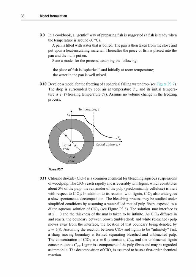
Trim: 247mm × 174mm Top: 12.653mm Gutter: 16.871mmCUUK2531-03 CUUK2531/Rasmuson ISBN: 978 1 107 04969 7 November 13, 2013 17:53
38 Model formulation
3.9 In a cookbook, a “gentle” way of preparing fish is suggested (a fish is ready whenthe temperature is around 60 °C).
A pan is filled with water that is boiled. The pan is then taken from the stove andput upon a heat-insulating material. Thereafter the piece of fish is placed into thepan and the lid is put on.
State a model for the process, assuming the following:
the piece of fish is “spherical” and initially at room temperature;the water in the pan is well mixed.
3.10 Develop a model for the freezing of a spherical falling water drop (see Figure P3.7).The drop is surrounded by cool air at temperature T∞ and its initial tempera-ture is Ti (˃freezing temperature T0). Assume no volume change in the freezingprocess.
Figure P3.7
3.11 Chlorine dioxide (ClO2) is a common chemical for bleaching aqueous suspensionsof wood pulp. The ClO2 reacts rapidly and irreversibly with lignin, which constitutesabout 5% of the pulp; the remainder of the pulp (predominantly cellulose) is inertwith respect to ClO2. In addition to its reaction with lignin, ClO2 also undergoesa slow spontaneous decomposition. The bleaching process may be studied undersimplified conditions by assuming a water-filled mat of pulp fibers exposed to adilute aqueous solution of ClO2 (see Figure P3.8). The solution–mat interface isat x = 0 and the thickness of the mat is taken to be infinite. As ClO2 diffuses inand reacts, the boundary between brown (unbleached) and white (bleached) pulpmoves away from the interface, the location of that boundary being denoted byx = δ(t). Assuming the reaction between ClO2 and lignin to be “infinitely” fast,a sharp moving boundary is formed separating bleached and unbleached pulp.The concentration of ClO2 at x = 0 is constant, CA0, and the unbleached ligninconcentration is CB0. Lignin is a component of the pulp fibres and may be regardedas immobile. The decomposition of ClO2 is assumed to be as a first-order chemicalreaction.
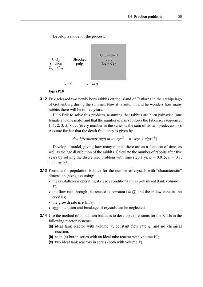
Trim: 247mm × 174mm Top: 12.653mm Gutter: 16.871mmCUUK2531-03 CUUK2531/Rasmuson ISBN: 978 1 107 04969 7 November 13, 2013 17:53
3.6 Practice problems 39
Develop a model of the process.
Figure P3.8
3.12 Erik released two newly born rabbits on the island of Tistlarna in the archipelagoof Gothenburg during the summer. Now it is autumn, and he wonders how manyrabbits there will be in five years.
Help Erik to solve this problem, assuming that rabbits are born pair-wise (onefemale and one male) and that the number of pairs follows the Fibonacci sequence:1, 1, 2, 3, 5, 8, . . . (every number in the series is the sum of its two predecessors).Assume further that the death frequency is given by
deathfrequency(age) = a · age2 − b · age + c[yr−1].
Develop a model, giving how many rabbits there are as a function of time, aswell as the age distribution of the rabbits. Calculate the number of rabbits after fiveyears by solving the discretized problem with time step 1 yr, a = 0.015, b = 0.1,and c = 0.3.
3.13 Formulate a population balance for the number of crystals with “characteristic”dimension (size), assuming:� the crystallizer is operating at steady conditions and is well mixed (tank volume =
V);� the flow-rate through the reactor is constant (= Q) and the inflow contains no
crystals;� the growth rate is v (m/s);� agglomeration and breakage of crystals can be neglected.
3.14 Use the method of population balances to develop expressions for the RTDs in thefollowing reactor systems:(a) ideal tank reactor with volume V, constant flow rate q, and no chemical
reaction;(b) as in (a) but in series with an ideal tube reactor with volume V1;(c) two ideal tank reactors in series (both with volume V).
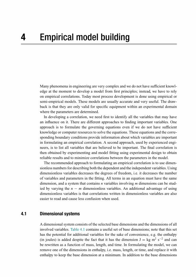
Trim: 247mm × 174mm Top: 12.653mm Gutter: 16.871mmCUUK2531-04 CUUK2531/Rasmuson ISBN: 978 1 107 04969 7 November 13, 2013 16:29
4 Empirical model building
Many phenomena in engineering are very complex and we do not have sufficient knowl-edge at the moment to develop a model from first principles; instead, we have to relyon empirical correlations. Today most process development is done using empirical orsemi-empirical models. These models are usually accurate and very useful. The draw-back is that they are only valid for specific equipment within an experimental domainwhere the parameters are determined.
In developing a correlation, we need first to identify all the variables that may havean influence on it. There are different approaches to finding important variables. Oneapproach is to formulate the governing equations even if we do not have sufficientknowledge or computer resources to solve the equations. These equations and the corre-sponding boundary conditions provide information about which variables are importantin formulating an empirical correlation. A second approach, used by experienced engi-neers, is to list all variables that are believed to be important. The final correlation isthen obtained by experimenting and model fitting using experimental design to obtainreliable results and to minimize correlations between the parameters in the model.
The recommended approach to formulating an empirical correlation is to use dimen-sionless numbers for describing both the dependent and the independent variables. Usingdimensionless variables decreases the degrees of freedom, i.e. it decreases the numberof variables and parameters in the fitting. All terms in an equation must have the samedimension, and a system that contains n variables involving m dimensions can be stud-ied by varying the n − m dimensionless variables. An additional advantage of usingdimensionless variables is that correlations written in dimensionless variables are alsoeasier to read and cause less confusion when used.
4.1 Dimensional systems
A dimensional system consists of the selected base dimensions and the dimensions of allinvolved variables. Table 4.1 contains a useful set of base dimensions; note that this sethas the potential for additional variables for the sake of convenience, e.g. the enthalpy(in joules) is added despite the fact that it has the dimension J = kg m2 s−2 and canbe rewritten as a function of mass, length, and time. In formulating the model, we canremove one of the dimensions in enthalpy, i.e. mass, length, or time, and replace it withenthalpy to keep the base dimension at a minimum. In addition to the base dimensions

Trim: 247mm × 174mm Top: 12.653mm Gutter: 16.871mmCUUK2531-04 CUUK2531/Rasmuson ISBN: 978 1 107 04969 7 November 13, 2013 16:29
4.2 Dimensionless equations 41
Table 4.1. A set of base dimensions
Variable Dimension SI units
Length L mMass M kgTime t sTemperature T KEnthalpy H JAmount of species N mole
Table 4.2. Dimensions of variables
Measured variable Dimension SI units
Force MLt−2 kg m s−2 = NPressure ML−1t−2 kg m−1 s−2 = PaPower ML2t−3 or Ht−1 kg m2 s−3 = J s−1 = WDensity ML−3 kg m−3
Surface tension Mt−2 kg s−2 = N m−1
in Table 4.1, there are several more variables that can be selected as base dimensions ifrequired, e.g. electric current (ampere) and magnetic field (gauss).
The dimensions of all variables can then be written as functions of the base variablesin Table 4.1, as seen in Table 4.2. Depending on the selection of base dimensions, thedimension can be written in different forms.
4.2 Dimensionless equations
All models we use in chemical engineering can be formulated in the dimensionlessform. The fundamental equations that describe the most phenomena in chemical engi-neering are formulated in Equations (4.1)–(4.5), and the involved variables are listedin Table 4.3. The characteristic dimensions are mass (M), length (L), time (t), enthalpy(H), temperature (T), and moles (N).
The momentum equation, Equation (4.1), together with the continuity equation, Equa-tion (4.2), describe the flow, and with the heat balance, Equation (4.4), and the speciesbalance, Equation (4.5), a complete system is described. However, this is a simplifiedexample because most source terms are not included.
Momentum balance
ρ
[∂v
∂t+ v · ∇v
]= μ∇2v + ρG − ∇ p
[kg
m2 s2
]. (4.1)
Equation of continuity
∂ρ
∂t= −[∇(ρv)]
[kg
m3 s
]. (4.2)

Trim: 247mm × 174mm Top: 12.653mm Gutter: 16.871mmCUUK2531-04 CUUK2531/Rasmuson ISBN: 978 1 107 04969 7 November 13, 2013 16:29
42 Empirical model building
Table 4.3. Variables involved in Equations (4.1)–(4.5)
Variable Physical property Characteristic dimension SI units
k thermal conductivity HL−1T−1t−1 J m−1 K−1 s−1
T temperature T KU velocity Lt−1 m s−1
L length L mρ density ML−3 kg m−3
μ viscosity ML−1t−1 kg m−1 s−1
cp specific heat HM−1T−1 J kg−1 K−1
C concentration NL−3 mol m−3
D diffusivity L2t−1 m2 s−1
As pressure is not an explicit variable in the momentum equation, the continuity equationis often rewritten by combining momentum balance and the continuity equation. Forconstant viscosity and density, the continuity equation can be replaced by the Poissonequation:
∇2 p = −∇ · ρv · ∇v
[Pa
m2= kg
m3 s2
]. (4.3)
Heat balance (without source terms)
ρcp
[∂T
∂t+ v · ∇T
]= ∇ · k∇T
[J
m3 s
]. (4.4)
Species balance (without source terms)
∂Ci
∂t+ v · ∇Ci = ∇ · D∇Ci
[mol
m3 s
]. (4.5)
Rewriting the governing equations in the dimensionless form simplifies the estimationof the behavior of processes on different scales. Since all terms in the equations havethe same dimensions, we can obtain a dimensionless equation by dividing the terms inthe equations by any of the other terms. However, dividing by the term that we assumeis the most important will simplify the analysis. In many cases, the convective term isthe dominating term. The tables in Appendix B show how the dimensionless variablesare formed from momentum, heat, and mass balances.
All variables must be scaled with a variable characteristic of the process. The char-acteristic velocity U may be the average inlet velocity. The characteristic length L maybe the tube diameter, the reactor length, or the catalyst particle diameter, depending onthe processes involved. Time may be scaled with residence time or the time constant fordiffusion.
Throughout the book we will be using ˆ to denote dimensionless variables, and wewill obtain
x = x
Land t = t
U
Lor t = t
D
L2. (4.6)

Trim: 247mm × 174mm Top: 12.653mm Gutter: 16.871mmCUUK2531-04 CUUK2531/Rasmuson ISBN: 978 1 107 04969 7 November 13, 2013 16:29
4.2 Dimensionless equations 43
Concentration is usually scaled with the total or inlet concentrations. The characteristictemperature may be inlet temperature, but it is often scaled with the minimum andmaximum temperatures to obtain a dimensionless variable between 0 and 1:
C = C
CT OTand T = T − Tmin
Tmax − Tmin= T − Tmin
�T. (4.7)
Gravity is important for buoyancy, and the maximal force caused by gravity due to thedifference in density is a suitable characteristic variable:
G = G
�ρg. (4.8)
The additional dimensionless dependent variables are formed from the characteristicvelocity and the pressure difference over the system:
v(x, t) = v(x, t)
Up(x, t) = p(x, t)
�p. (4.9)
The Reynolds, Euler, Froude, and Peclet numbers,
Re = ρU L
μ, Eu = �p
ρU 2, Fr = gL�ρ
ρU 2, PeH = U L
α, PeD = U L
D,
are dimensionless numbers that are most often used in formulating the transport equa-tions, Equations (4.1)–(4.5), in the dimensionless form. The Peclet number for heat con-duction, PeH = U L/α, with thermal diffusion α = k/ρcP , has a corresponding Pecletnumber for diffusion, PeD = U L/D. It is often convenient to separate the dimensionlessvariables into variables that describe the properties of a flow and a fluid. The Prandtl andSchmidt numbers are useful dimensionless variables that describe the fluid propertiesheat conduction and diffusion, respectively:
Pr = cpμ
kand Sc = μ
ρD. (4.10)
Note that the Peclet number can also be formulated as a product of the Reynolds number,i.e.
PeH = Re · Pr and PeD = Re · Sc. (4.11)
By multiplying Equations (4.1)–(4.5) by L/U and substituting the dependent variableswith corresponding dimensionless variables, we obtain the following dimensionlessequations.
Momentum balance
∂ v
∂ t+ v · ∇v = 1
Re∇2v + 1
FrG − 1
Eu∇ p. (4.12)
Equation of continuity
∇2 p = − 1
Eu∇ · v · ∇v. (4.13)
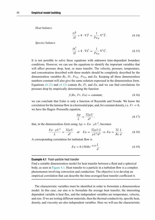
Trim: 247mm × 174mm Top: 12.653mm Gutter: 16.871mmCUUK2531-04 CUUK2531/Rasmuson ISBN: 978 1 107 04969 7 November 13, 2013 16:29
44 Empirical model building
Heat balance
∂ T
∂ t+ v · ∇ T = 1
PeH∇2T . (4.14)
Species balance
∂C
∂ t+ v · ∇C = 1
PeD∇2C . (4.15)
It is not possible to solve these equations with unknown time-dependent boundaryconditions. However, we can use the equations to identify the important variables thatwill affect pressure drop, heat, or mass transfer. The velocity, pressure, temperature,and concentration described with these models should be completely described by thedimensionless variables Re, Fr, PeH , PeD , and Eu. Keeping all these dimensionlessnumbers constant will also give the same solution expressed in the dimensionless form.Equations (4.12) and (4.13) contain Re, Fr, and Eu, and we can find correlations forpressure drop by empirically determining the function
f (Re, Fr, Eu) = constant; (4.16)
we can conclude that Euler is only a function of Reynolds and Froude. We know thecorrelation for the laminar flow in a horizontal pipe, and, for constant density, i.e. Fr = 0,we have the Hagen–Poiseuille equation,
�p
L= 32μU
d2, (4.17)
that, in the dimensionless form using �p = Eu · ρU 2, becomes
Eu · ρU 2
L= 32μU
d2or Eu = 32μU L
ρU 2d2⇒ Eu = 32
Re
L
d. (4.18)
A corresponding correlation for turbulent flow is
Eu = 0.158Re−0.25 L
d. (4.19)
Example 4.1 Fluid–particle heat transferFind a suitable dimensionless model for heat transfer between a fluid and a sphericalbody, as seen in Figure 4.1. Heat transfer to a particle in a turbulent flow is a complexphenomenon involving convection and conduction. The objective is to develop anempirical correlation that can describe the time-averaged heat transfer coefficient h.
The characteristic variables must be identified in order to formulate a dimensionlessmodel. In this case, our aim is to formulate the average heat transfer; the interestingdependent variable is heat flux, and the independent variables are temperature, velocity,and size. If we are testing different materials, then the thermal conductivity, specific heat,density, and viscosity are also independent variables. Here we will use the characteristic

Trim: 247mm × 174mm Top: 12.653mm Gutter: 16.871mmCUUK2531-04 CUUK2531/Rasmuson ISBN: 978 1 107 04969 7 November 13, 2013 16:29
4.2 Dimensionless equations 45
Figure 4.1. Heat transfer to a spherical particle.
length L as the diameter of the sphere and the characteristic velocity U as the velocityfar from the body. The characteristic temperature is set as the difference between thebulk temperature and the surface temperature, i.e. �T = Tb − Tw. Time is not relevanthere, but is discussed in Section 5.1.5. The governing equations and the characteristicdimensions are written in the following using particle diameter as the characteristiclength L = d.
The film theory describes heat transfer to the surface. The heat flux modeled usingthe heat transfer coefficient is balanced with the flux into the solid sphere:
q = h(Tb − TW ) = kdT
dr
∣∣∣∣r=R
[J
m2 s
]. (4.20)
Defining T = (T − Tb)/�T and r = r/(d/2) with Nu = h · d/k, we obtain, afterdividing by �T and h, the dimensionless equation for heat transfer to the surface.
Heat transfer at the particle surface
1 = 1
Nu
∂ T
dr
∣∣∣∣∣r=1
. (4.21)
Removing the transient part from Equations (4.12)–(4.14) gives the remainingequations.
Momentum balance
v · ∇v = 1
Re∇2v + 1
FrG − 1
Eu∇ p. (4.22)
Equation of continuity
∇2 p = − 1
Eu∇v · ∇v. (4.23)
Heat balance
v · ∇ T = 1
PeH∇2T . (4.24)

Trim: 247mm × 174mm Top: 12.653mm Gutter: 16.871mmCUUK2531-04 CUUK2531/Rasmuson ISBN: 978 1 107 04969 7 November 13, 2013 16:29
46 Empirical model building
Velocity and pressure are determined from Equations (4.22)–(4.23), i.e. Eu =f (Re, Fr ). For simplicity, we can assume that there are no density differences, andthe term containing the Froude number can be neglected. Only Nu, Re, Eu, and PeH
remain, and as Eu = f (Re) the Nusselt number Nu must be a function of Re and PeH .However, in most empirical correlations, the Prandtl number, Pr, is preferred insteadof the Peclet number, PeH , but as Pr = PeH/Re no new dimensionless variables areintroduced:
Nu = b0 + b1 Reα1 Prβ1 + b2 Reα2 Prβ2 + · · · . (4.25)
The parameters b0, αi , and βi are determined from experimental data. One commoncorrelation is the Frossling/Ranz–Marshall correlation,
Nu = 2 + 0.6Re1/2 Pr1/3. (4.26)
Using dimensionless variables allows for the development of scale-independent designequations. Note that the species balance equation is almost identical to the heat balance,and that, by replacing the Pr number in Equation (4.25) with the Schmidt number Sc,we obtain a similar correlation for mass transfer as for heat transfer. In principle theydescribe similar phenomena, and, if we replace heat conduction k with heat diffusionα = k/ρcp containing the same dimension as diffusivity (m2 s−1), we obtain the sameexpression.
Many different dimensionless numbers can be obtained by simply dividing the termsin any dimensional consistent equation, as seen in the Appendix B. The most commonlyused dimensionless numbers are listed in Table B.4.
4.3 Empirical models
The dimensionless form is also suitable for developing models or correlations thathave a less theoretical basis and cannot be deduced from simple balance equations. Theadvantage of using dimensionless variables is that, if there are any n variables containingm primary dimensions, the correlation can be formulated using n − m dimensionlessgroups. However, we need experience or some preliminary experiments to identify thevariables that are important.
To illustrate this method, we will use Example 4.1 with heat transfer to a particle or awall. Fluid solid heat transfer can be modeled as in Equation (4.20) as follows:
q = h(Tb − TW ) = kdT
dr
∣∣∣∣r=R
. (4.20)
The objective is to develop a model that can predict the heat transfer coefficient hor the Nusselt number. Equation (4.20) says nothing about the heat transfer coefficienth, and we need to conduct experiments to develop a model of heat flux that includesconvection, heat conduction, viscosity, heat capacity, etc., so that we can predict the

Trim: 247mm × 174mm Top: 12.653mm Gutter: 16.871mmCUUK2531-04 CUUK2531/Rasmuson ISBN: 978 1 107 04969 7 November 13, 2013 16:29
4.3 Empirical models 47
Table 4.4. Basic dimensions as functions of the variablesin the recurring set of variables
Variables Dimension SI units
Length L = l mMass M = ρl3 kgTime t = ρl2μ−1 sTemperature T = �T KEnthalpy H = kl3ρμ−1�T J
Nusselt number. In formulating a general correlation, we can list all variables that webelieve will affect heat transfer:
q = f (k,�T, u, l, ρ, μ, cp, βg). (4.27)
These n variables have dimensions in length L (m), mass M (kg), time t (s), temperatureT (K), and enthalpy H (J). The variables with their dimensions are listed in Table 4.3.In contrast to Example 4.1, we allow free convection, and an additional variable βgdescribes the effect of gravity on free convection. The thermal expansion coefficient β
describes how fluid density changes with temperature, e.g. for an ideal gas β = 1/T . Acorrelation for heat transfer should include these variables in a dimensional consistentform.
The dimensionless variables can be found by selecting m variables as a recurringset. These variables should contain the different variables that form a complete setof dimensions, i.e. it should not be possible to formulate a dimensionless variableby combining the variables in the recurring set. Here we will select l, ρ, μ,�T, k asthe recurring set. They are listed with their dimensions in Table 4.4. The selection ofvariables is not critical, and other combinations of variables containing length, mass,time, temperature, and enthalpy that could form the recurring set of variables are possible.
Selecting l, ρ, μ,�T, k as the recurring set leaves the n − m variables q, U, βg, cp asthe non-recurring variables. Using the dimensions in Table 4.4, the dimensional variablesare then identified as functions of the recurring variables. The non-recurring variablesq [J m−2 s−1], U [m s−1], cp [J kg K−1], and βg [m s−2 K−1] can be reformulated intodimensionless variables, e.g. q [J m−2 s−1] can be made dimensionless by dividing byenthalpy H (J) and multiplied by length (L2) and time (t). After replacing H, L, and t bythe variables in Table 4.4 and q by h�T, we obtain
�1 = qL2t
H= q(l2)(ρl2/μ)
(kl3ρ�T/μ)= ql
k�T
h
h= hl
k= Nu,
�2 = u
Lt= Uρl
μ= Re,
(4.28)�3 = cpMT
H= cpμ
k= Pr,
�4 = βgt2T
L= βg�Tρ2l3
μ2= Gr.

Trim: 247mm × 174mm Top: 12.653mm Gutter: 16.871mmCUUK2531-04 CUUK2531/Rasmuson ISBN: 978 1 107 04969 7 November 13, 2013 16:29
48 Empirical model building
The use of � as the symbol dimensionless variables was introduced by Buckingham,and this method has been called Buckingham’s � theorem since then. This is a verygeneral and useful method, but it will not guarantee the most physical meaningfulcorrelation.
According to Equation (4.27), heat flux should be a function of the remaining variables,which allows us to write the dimensionless heat flux as a function of the remainingdimensionless numbers:
�1 = f (�2,�3,�4) or Nu = f (Re, Pr, Gr ). (4.29)
The dimensionless analysis tells us nothing about the correlation; it only reveals whichvariables are involved. The final correlations can be formulated in many different ways.An empirical model for heat transfer may be formulated as
Nu = b0 + b1 Reα1 Prβ1 Grγ1 + b2 Reα2 Prβ2 Grγ2 + · · · , (4.30)
and the parameters bi, αi, β i, and γ i can be fitted from measurements. The dimension-less number Gr includes the effect of buoyancy. For heat transfer to a sphere in Exam-ple 4.1, with no buoyancy, the following empirical model has been found, as shownpreviously:
Nu = 2 + 0.6Re1/2 Pr1/3; (4.26)
for free convection on a vertical wall,
Nu = 0.68 + 0.67Ra1/4
[1 + (0.492/Pr )9/16]4/9, (4.31)
where Ra = Gr · Pr.
4.4 Scaling up
Scaling up equipment is a general problem in chemical engineering. If we were runningall processes at thermodynamic equilibrium, there would be no scaling-up problemand the final composition could be calculated from thermodynamic data. However, thissolution would require infinitely large equipment, and the thermodynamic equilibriummay not be the composition we want. In industrial production we aim for maximumproduction in the plant whilst keeping the quality of the product high. In scaling upwe cannot maintain the same conditions on all scales, e.g. surface/volume will decreasewith increasing size. Thus we introduce limitations on mass and heat transfer, and cannotexpect the same results on the industrial production scale as on the laboratory scale.
Before we build an industrial-scale process, we need to use the laboratory- andpilot-plant-scale equipment to develop an understanding of how the industrial-scaleproduction plant will work. The models we develop on smaller scales must be scalableand applicable to the large scale.
In general, we can separate the three different cases: scaling up, scaling down, andscaling out. In scaling up, we aim for building new equipments and will use experiments

Trim: 247mm × 174mm Top: 12.653mm Gutter: 16.871mmCUUK2531-04 CUUK2531/Rasmuson ISBN: 978 1 107 04969 7 November 13, 2013 16:29
4.4 Scaling up 49
on a small scale to develop models that are scale independent and can be used fordesigning the full-scale equipment. In scaling down, we already have the large-scaleequipment that we want to optimize for a new process. In such a case, we want to knowhow to design and run a pilot plant to mimic the behavior of a large-scale plant in order tofind the optimal conditions for it. In scaling out, we build a large-scale plant by puttingthe small-scale equipment in parallel. We then expect to obtain the same conditionsin the large scale as in the small scale. This can be done by, e.g., using small tubularreactors in parallel instead of building a large tubular reactor. The scaling-up problemis then limited to obtaining the same flow rate in all tubes and sufficient heat control ofthe tube bundle to keep the temperature equal.
The fundamental principle in scaling models is to keep all dimensionless variablesconstant. The dimensionless equations, e.g. Equations (4.12)–(4.15), are scale indepen-dent, and keeping Re, Pr, Eu, and Fr numbers constant results in dimensionless variablesv, G, p, T , and C versus t that is the same at all scales. In the simplest case, scaling witha constant Re, i.e. an increase in length scale by a factor of 10, requires that the charac-teristic velocity decreases by a factor of 10. As a result, assuming no density difference,i.e. Fr = 0, Eu will be constant and the pressure drop is scaled with ρU 2. Keeping Reand Pr constant should also result in the same dimensionless heat transfer coefficient,i.e. the Nusselt number, as obtained in the dimensionless correlations in Example 4.1.
For free convection problems, the Froude number must also be kept constant. Sincewe cannot change gravity, the density change with temperature and �ρ/ρ must beincreased. This might be very difficult while keeping Re and Pr constant.
More complex phenomena require keeping more dimensionless variables constant.A more complete heat flux balance will contain more terms, and consequently moredimensionless variables must be kept constant:
ρcpv · ∇T = ∇ · k∇T + rA�H + ha�T + eσ T 3�T . (4.32)convection conduction reaction phase transfer radiation
Dividing by ρcpU�TL, we obtain
v · ∇ T = 1
Pe∇2T + 1
DaI I IrA + Nu
RePrT + eσ T 3L
ρcpUT . (4.33)
In addition to the dimensionless variables for flow, Re, Fr, and Eu, we also need to keepPe, Nu, DaIII, and eσ T 3L/ρcpU constant to obtain the same dimensionless predictedconditions, i.e. Re = ρU L/μ, Pr = μ/ρα, Eu = �P/ρU 2, Fr = gL�ρ/ρU 2, Pe =ρcpU L/k, Nu = hL/k, DaI I I = rAL�H/ρC pU�T , and eσ T 3L/ρcpU should bekept constant.
We quickly reach a level of complexity that makes it impossible to keep all dimen-sionless variables constant. Using correlations developed on a small scale to predict thebehavior on the large scale may not be a good solution, because empirical correlationsare only correlations and as such are only valid within the range of experiments thatform the basis for the correlations. As not all the dimensionless variables could be keptconstant on all scales in our example, no experimental data from the small scale are

Trim: 247mm × 174mm Top: 12.653mm Gutter: 16.871mmCUUK2531-04 CUUK2531/Rasmuson ISBN: 978 1 107 04969 7 November 13, 2013 16:29
50 Empirical model building
Figure 4.2. Scaling up of stirred tank reactors.
valid for the large scale. Even if the correlations are written in the dimensionless form,this limitation must be kept in mind.
The next part of the procedure is to identify the rate-determining step, and determinewhich conditions should be scale similar. All the dimensionless variables may not beimportant. There are no general methods for finding the rate-determining steps, and agenuine understanding of the actual processes is needed. Detailed knowledge of specificprocesses is beyond the scope of this book. However, the example below will illustratethis approach.
Example 4.2 Mixing and reaction in a stirred tank reactorAssume that the chemical reaction A + B → products is scaled up from a 10 l pilotplant to 10 m3 full-scale production unit. Temperature control is usually a minorproblem in stirred tank reactors; instead the critical property is the rate of mixing. Thecharacteristic reaction time can be estimated from the kinetics and the concentration asfollows:
r = k(T ) · f (CA, CB)
[mol
m3 s
]and τreact = Climit
r[s],
where Climit is the concentration of the limiting reactant.
The rate-limiting steps may be the kinetics, but the macro- or micromixing canalso be rate limiting. A general approach to this problem requires that a large number ofdimensionless variables be kept constant. If the rate-determining step(s) can be identified,the scale-up process is easier.
In a very slow chemical reaction, the time for mixing is much faster than the reac-tion rate. The process is only dependent on species concentration and temperature.Keeping these constant during scale-up will result in the same production per volume

Trim: 247mm × 174mm Top: 12.653mm Gutter: 16.871mmCUUK2531-04 CUUK2531/Rasmuson ISBN: 978 1 107 04969 7 November 13, 2013 16:29
4.4 Scaling up 51
reactor. However, the surface area per volume will decrease with size, and additionalcooling/heating coils may be required.
In a slow chemical reaction, the flow circulation time in the reactor is on the same timescale as the chemical reaction time, which will lead to variations in concentration withinthe reactor. Scaling up with constant circulation times would be a proper scaling-up rule.However, the flow must be turbulent in both cases, or the mixing time will increase byseveral orders of magnitude.
The pumping capacity of an impeller is proportional to the impeller tip speed N · π · dand the swept area of the impeller tip π · d · h. Here, N is the impeller speed, d is theimpeller diameter, and h is the height of the impeller blades. Assuming that the impellerblades scale with the reactor size, D, we can assume that d�D and h�D are constant onall scales, and consequently the pumping rate is given by
Q ∝ Nπd · πd · h ∝ ND3 [m3 s−1], (4.34)
and, following the scaling-up rule with a constant pumping rate per volume reactor,circulation time is given by
τcirc ∝(
D3
ND3
)large
=(
D3
ND3
)small
or τcirc ∝(
1
N
)large
=(
1
N
)small
. (4.35)
This scaling rule indicates that the impeller speed should be kept constant. However,the energy input from the impeller scales with N3D5, as shown in Practice problem4.3, and at constant impeller speed the required power input scales as (Dlarge/Dsmall)5.An increase by a factor of 10 in linear dimension will require an increase by a factorof 105 in power input. This is usually not possible to obtain, and a larger variation inconcentration will occur on the large scale.
Fast chemical reactions are affected by the mixing on the smallest scale. The turbulentproperties together with the kinetics determine the outcome. The turbulence is generatedby the impeller, but turbulence is also dissipated much faster in the impeller region. Thiswill lead to two very different regions in the reactor: the impeller region with very fastmixing and reaction, and the remaining volume with very slow mixing and reaction.
The mixing time for fast reactions scales with the lifetime of the turbulent eddies k�ε
or, for more viscous, fluids as√
ν/ε, where k is the turbulent kinetic energy, ε is the rateof dissipation, and ν is the kinematic viscosity. The kinetic energy scales as the impellertip speed squared, i.e. k ∝ (ND)2, and the dissipation scales as power input per volume,ε ∝ P/V ∝ N 3 D5/D3 = N 3 D2. The micromixing time is then estimated as
τmicro ∝ k
ε∝ N 2 D2
N 3 D2= 1
Nor τmicro ∝
√ν
ε∝ N−3/2 D−1. (4.36)
Keeping k�ε constant requires the same impeller speed on all scales, and consequentlywe obtain the same problem with power input as for constant circulation time. Constantε requires that when size D increases, the impeller speed should decrease as
Nlarge = Nsmall
(Dsmall
Dlarge
)2/3
. (4.37)

Trim: 247mm × 174mm Top: 12.653mm Gutter: 16.871mmCUUK2531-04 CUUK2531/Rasmuson ISBN: 978 1 107 04969 7 November 13, 2013 16:29
52 Empirical model building
Here we have assumed that the turbulent kinetic energy and the dissipation rateare the same throughout the whole reactor. However, stirred tank reactors are veryheterogeneous, with much higher kinetic energy and a higher dissipation rate in theimpeller region than in the rest of the tank. This makes stirred tank reactors very difficultto scale-up. Reactors containing packed beds, metal foams, or static mixers are mucheasier to scale-up since the flow, mass transfer, and reactions are much more similar onthe small and large scales.
4.5 Practice problems
4.1 The Ergun equation for pressure drop in porous beds is given by
�P
L= −AμU − B
(1
2ρU 2
), (4.38)
with
A = 150(1 − α)2
d2pα
3and B = 1.75(1 − α)
dpα3,
where α is the void fraction.Show that the pressure drop can be written in the form
Eu = b0 + b1 Reβ1 + b2 Reβ2 .
4.2 Derive an expression for the Sherwood number as a function of Re and Sc usingEquations (4.12), (4.13), and (4.15), and suitable boundary conditions.
4.3 The power input per unit volume in a stirred tank reactor depends on liquid density,the impeller diameter, and speed, i.e. P = f (ρ, D, N ). Write a dimensionlessrelation between power input and these variables. Assume that the impeller and tanksize have a constant ratio, and only one characteristic length, the impeller diameterD, is needed.
4.4 In boiling, the heat transfer coefficient h [W m−2 K−1] depends on the heat flux q [Wm−2], thermal conductivity k [W m−1 K−1], latent heat of vaporization λ [J kg−1],viscosity μ [kg m−1 s−1], surface tension σ [J m−2], pressure, P [N m−2], bubblediameter d [m], liquid density ρ [kg m−3], and the density difference between liquidand vapor �ρ [kg m−3]:
h = f (q, k, μ, σ, P, d, ρ,�ρ).
Formulate a model for the heat transfer coefficient (Nusselt number) with theminimum number of dimensionless variables.

Trim: 247mm × 174mm Top: 12.653mm Gutter: 16.871mmCUUK2531-05 CUUK2531/Rasmuson ISBN: 978 1 107 04969 7 November 13, 2013 16:30
5 Strategies for simplifyingmathematical models
A mathematical model can never give an exact description of the real world, and thebasic concept in all engineering modeling is, “All models are wrong – some models areuseful.” Reformulating or simplifying the models is not tampering with the truth. Youare always allowed to change the models, as long as the results are within an acceptablerange. It is the objective of the modeling that determines the required accuracy: Is it aconceptual study limited to order of magnitude estimations? Or is it design modeling inwhich you will add 10–25% to the required size in order to allow for inaccuracies in themodels and future increase in production? Or is it an academic research work that youwill publish with as accurate simulations as possible?
A simulation may contain both errors and uncertainties. An error is defined as arecognizable deficiency that is not due to lack of knowledge, and an uncertainty is apotential deficiency that is due to lack of knowledge. All simulations must be validatedand verified in order to avoid errors and uncertainties. Validation and verification are twoimportant concepts in dealing with errors and uncertainties. Validation means makingsure that the model describes the real world correctly, and verification is a procedure toensure that the model has been solved in a correct way.
Poor simulation results are due to many different reasons:
� errors in formulating the problem;� inaccurate models;� inaccurate data on the physical properties;� numerical errors due to the choice of numerical methods;� lack of convergence in the simulations.
It is always recommended that you do simple by-hand calculations to define the propertiesof the system prior to formulating the final model. The objective of this chapter is topresent strategies for simplifying given mathematical models and for reducing the modelsalready in the formulation.
Many models in chemical engineering are derived from four basic balance equations,as seen in Chapter 4, but now we have also included the source terms for chemicalreactions and heat formation.
Material balance
∂ CA
∂ t+ v · ∇CA = ∇ · DA∇CA − RA. (5.1)

Trim: 247mm × 174mm Top: 12.653mm Gutter: 16.871mmCUUK2531-05 CUUK2531/Rasmuson ISBN: 978 1 107 04969 7 November 13, 2013 16:30
54 Strategies for simplifying mathematical models
Heat balance
ρcp
[∂ T
∂ t+ v · ∇T
]= ∇ · k∇T + Q. (5.2)
Momentum balance
ρ
[∂ v
∂ t+ v · ∇v
]= μ∇2v + ρ G − ∇ p. (5.3)
Equation of continuity
∂ ρ
∂ t= −[∇(ρv)], (5.4)
with suitable initial and boundary conditions.There are general programs that can solve these equations for simple systems, e.g.
computational fluid dynamics, CFD. However, the equations can easily become verydifficult if they include stiff non-linear equations and complex geometry that call for astructured approach.
5.1 Reducing mathematical models
Equations (5.1)–(5.4) describe many systems in chemical engineering. But the equationsdo not contain the true nature of the real world; they are merely convenient mathematicalapproximations of our models of the real world.
These complex mathematical models are in many cases difficult to solve. A verygood work station is necessary for solving 3D flows in a reactor with an exothermicchemical reaction. If we want to solve the equations for a heterogeneous system, acomputer cluster is required that can give a solution within a reasonable time. Yet inmany cases the equations can be reduced without losing too much accuracy. In somecases, even a better numerical precision can be reached. The following list covers someof the most commonly used methods for reducing the computational efforts for solvingmathematical equations.
� decoupling equations;� reducing the number of independent variables;� averaging over time or space “lumping”;� simplifying geometry;� separating equations into steady state and transient;� linearizing;� solving for limiting cases;� neglecting terms;� changing boundary conditions.

Trim: 247mm × 174mm Top: 12.653mm Gutter: 16.871mmCUUK2531-05 CUUK2531/Rasmuson ISBN: 978 1 107 04969 7 November 13, 2013 16:30
5.1 Reducing mathematical models 55
5.1.1 Decoupling equations
Decoupling equations is one of the most important tools for reducing complex math-ematical models. A model with many dependent variables, e.g. different velocities,concentrations of chemical substances, and temperature, can be simplified substantiallyif we look for variables that are not dependent on the others. In Equations (5.1)–(5.4),the coupling occurs mainly through the velocity in all the equations and through temper-ature. The reaction rate in Equation (5.1) depends on temperature, and the temperaturein Equation (5.2) depends on the reaction rate through the heat of the reaction. Viscosityand density of the fluid also depend on temperature and chemical composition, and as aconsequence all reactions must be solved simultaneously. On the contrary, if the heat ofthe reaction is low, the temperature variation will be small, the fluid density and viscositycan be assumed constant, and the flow may be calculated in advance. In such a case, thechemical reactions can then be added to a precalculated velocity distribution.
Coupling may also occur via boundary conditions, e.g. the reaction rate in a cata-lyst pellet depends on the concentration and the temperature of the fluid surroundingthe pellet. At steady state, when coupling between equations occurs through boundaryconditions, an exact or approximate analytical solution can be calculated with boundaryconditions as variables, e.g. the effectiveness factor for a catalyst particle can be formu-lated as an algebraic function of surface concentrations and temperature. The reactionrate in the catalyst can then be calculated using the effectiveness factor when solving thereactor model. However, this is not possible for transient problems. The transport in andout of the catalyst also depends on the accumulation within the catalyst, and the actualreaction rate depends on the previous history of the particle.
A very efficient method is to precalculate steady-state solutions and save the resultsin look-up tables. Interpolation in multidimensional look-up tables is most often muchfaster than iterative solutions of non-linear equations. It is also possible to use look-uptables for initial-value differential equations using time as one variable in the look-uptable.
Decoupling equations may also be used to enhance the numerical stability of stationaryproblems even when the equations have strong coupling. You can start by solving, e.g.,the flow field and then continue with species, reactions, and heat, and finally solve theflow field, species, and heat with updated properties for concentrations, temperature,density, and viscosity. This control of the iterations allows for a more stable approach tothe final solution.
5.1.2 Reducing the number of independent variables
By reducing the number of independent variables, e.g. space or time, a partial differ-ential equation can, in the best case, be reduced to an ordinary differential equation oreven an algebraic equation, and the computational effort is reduced substantially. Themost obvious approach is to use the symmetry in geometry. Spherical and cylindricalsymmetry is often easy to find. This will reduce a 3D problem to a 1D or 2D problemwith a significant decrease in computational time.
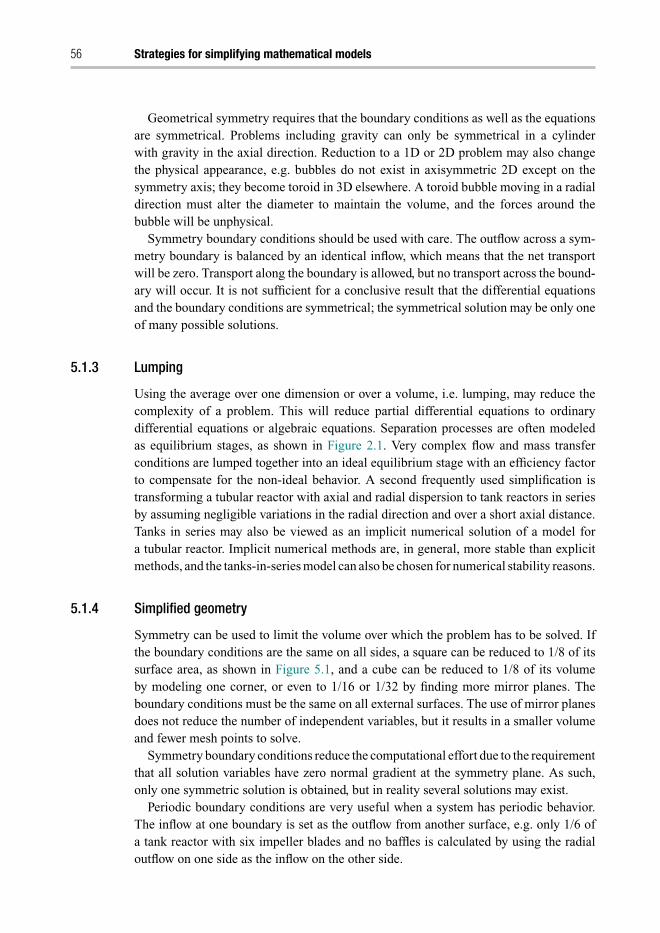
Trim: 247mm × 174mm Top: 12.653mm Gutter: 16.871mmCUUK2531-05 CUUK2531/Rasmuson ISBN: 978 1 107 04969 7 November 13, 2013 16:30
56 Strategies for simplifying mathematical models
Geometrical symmetry requires that the boundary conditions as well as the equationsare symmetrical. Problems including gravity can only be symmetrical in a cylinderwith gravity in the axial direction. Reduction to a 1D or 2D problem may also changethe physical appearance, e.g. bubbles do not exist in axisymmetric 2D except on thesymmetry axis; they become toroid in 3D elsewhere. A toroid bubble moving in a radialdirection must alter the diameter to maintain the volume, and the forces around thebubble will be unphysical.
Symmetry boundary conditions should be used with care. The outflow across a sym-metry boundary is balanced by an identical inflow, which means that the net transportwill be zero. Transport along the boundary is allowed, but no transport across the bound-ary will occur. It is not sufficient for a conclusive result that the differential equationsand the boundary conditions are symmetrical; the symmetrical solution may be only oneof many possible solutions.
5.1.3 Lumping
Using the average over one dimension or over a volume, i.e. lumping, may reduce thecomplexity of a problem. This will reduce partial differential equations to ordinarydifferential equations or algebraic equations. Separation processes are often modeledas equilibrium stages, as shown in Figure 2.1. Very complex flow and mass transferconditions are lumped together into an ideal equilibrium stage with an efficiency factorto compensate for the non-ideal behavior. A second frequently used simplification istransforming a tubular reactor with axial and radial dispersion to tank reactors in seriesby assuming negligible variations in the radial direction and over a short axial distance.Tanks in series may also be viewed as an implicit numerical solution of a model fora tubular reactor. Implicit numerical methods are, in general, more stable than explicitmethods, and the tanks-in-series model can also be chosen for numerical stability reasons.
5.1.4 Simplified geometry
Symmetry can be used to limit the volume over which the problem has to be solved. Ifthe boundary conditions are the same on all sides, a square can be reduced to 1/8 of itssurface area, as shown in Figure 5.1, and a cube can be reduced to 1/8 of its volumeby modeling one corner, or even to 1/16 or 1/32 by finding more mirror planes. Theboundary conditions must be the same on all external surfaces. The use of mirror planesdoes not reduce the number of independent variables, but it results in a smaller volumeand fewer mesh points to solve.
Symmetry boundary conditions reduce the computational effort due to the requirementthat all solution variables have zero normal gradient at the symmetry plane. As such,only one symmetric solution is obtained, but in reality several solutions may exist.
Periodic boundary conditions are very useful when a system has periodic behavior.The inflow at one boundary is set as the outflow from another surface, e.g. only 1/6 ofa tank reactor with six impeller blades and no baffles is calculated by using the radialoutflow on one side as the inflow on the other side.

Trim: 247mm × 174mm Top: 12.653mm Gutter: 16.871mmCUUK2531-05 CUUK2531/Rasmuson ISBN: 978 1 107 04969 7 November 13, 2013 16:30
5.1 Reducing mathematical models 57
Figure 5.1. Symmetry in a square.
Figure 5.2. Simplified geometry. When only the outer part of a complex body is active, the bodymay be simplified to a slab.
In many cases, irregular-shaped particles or a size distribution of particles can betreated as spheres with an equivalent diameter that gives the same surface/volume ratioas the irregular-shaped particle. The Saunter mean diameter, usually denoted d32, definedas the total volume divided by the total surface area, is a very common method used tocharacterize a size distribution of bubbles or drops. With this definition, the total volumecan be calculated from the number of particles multiplied by the volume of a sphere withdiameter d32, and the total surface area can be calculated by multiplying the number ofparticles by the surface of the sphere.
The use of hydraulic diameter in calculating pressure drop is a commonly usedconcept for simplifying geometry. The hydraulic diameter for an opening is calculatedby multiplying the open surface area by 4, then dividing by the wetted periphery, e.g.for a cylindrical opening d = 4(πd2/4)/(πd), and for a square duct d = 4d2/(4d).
It is not necessary to solve the complete geometry if only part of a volume is involvedbased on the concept that “the earth is locally flat.” For example, a very fast chem-ical reaction in an irregular-shaped catalyst will involve only the outer surface, andtherefore the catalyst may be treated as a slab with a surface A, equal to the particlesurface and thickness δ, which is sufficient for containing all interesting phenomena (seeFigure 5.2).

Trim: 247mm × 174mm Top: 12.653mm Gutter: 16.871mmCUUK2531-05 CUUK2531/Rasmuson ISBN: 978 1 107 04969 7 November 13, 2013 16:30
58 Strategies for simplifying mathematical models
5.1.5 Steady state or transient
When different parts of a process have very different time dependencies, the fast varyingvariables can be treated as steady-state variables when solving for the slow variables.Similarly, the slowly varying variables can be considered constant when solving forthe fast varying variables. Time constants are very convenient tools for estimatingtime dependence. Assuming a pseudo-steady state for a complex reaction sequence,e.g. combustion involving hundreds of reactions, is a useful method for decreasing thenumber of ordinary differential equations that must be solved by transforming them intoalgebraic equations. “Pseudo-steady state” means that the whole process is unsteady,but some sequences of the process change very fast, and the accumulation term in thatstep can be neglected. This is valid for many radicals in complex chemical reactions.The radicals react very quickly and have very low concentrations, because once they areformed they will react further.
Estimating the time constants for convection is straightforward. The residence timeis estimated from length and velocity, t = L/v, or from volume and volumetric flow,t = V/q. Transport by diffusion is more difficult to estimate. Solving the unsteadytransport equation for diffusion, Equation (5.5), heat conduction, or viscous transportfor transport into a slab will give information about two things: the time needed to bringabout a change in boundary conditions to affect the whole volume, or how far, into aninfinite slab species, heat or momentum can penetrate within a given time.
Unsteady diffusion in a slab is described by
∂C
∂t= D
∂2C
∂z2, (5.5)
which in dimensionless form is
∂ y
∂ t= ∂2 y
∂ z2, (5.6)
with
x = x
L, y = C
C(z = 0), t = t D
L2.
Equation (5.6) can also describe heat transfer and slow viscous flow using
y = T − Tinit
T (z = 0) − Tinit, t = tλ
ρcp L2
for heat and
y = U
U (z = 0), t = tμ
ρL2
for velocity. The boundary conditions with constant concentration on one side and notransport out on the other side,
y = 1 at z = 0 andd y
dz= 0 at z = 1,

Trim: 247mm × 174mm Top: 12.653mm Gutter: 16.871mmCUUK2531-05 CUUK2531/Rasmuson ISBN: 978 1 107 04969 7 November 13, 2013 16:30
5.1 Reducing mathematical models 59
Figure 5.3. Time constants for diffusion in a slab with different boundary conditions. (a) No fluxat z = 1; (b) y(t, ∞) = 0.
together with the initial conditions
y(0, z) = 0,
describe a step change at the boundary from 0 to 1, and Equation (5.6) has the solution
y(t, z) =∞∑
i=0
(−1)i
[erfc
(z − 2i
2√
t
)+ erfc
(2i + 2 − z
2√
t
)]. (5.7)
From Figure 5.3(a) we can see that steady state at y = 1 is reached when t � 1,i.e. t = Dt/L2 � 1 or t � L2/D. It is also very convenient to define dimensionlesstime as t = t/τ using the time constants τ = L2/D, τ = ρcp L2/λ, and τ = ρL2/μ
for diffusion, heat conduction, and the viscous transport of momentum, respectively.In Figure 5.3(a), y is close to 1 when t = 1, and in this case we can, with reasonableconfidence, assume steady state when t > τ .
Information about how far the species will penetrate as a function of time is obtainedby changing the boundary condition at z = 1 for Equation (5.6) to y(t,∞) = 0. Thisboundary condition gives the solution
y(t, z) = 1 − erf
(z
2√
t
). (5.8)
The result is shown in Figure 5.3(b). As y depends only on z/√
4t , there is a linearrelation between z and
√t at constant y, and putting z/
√t = 1, i.e. z = √
Dt , will yielda constant value of y = 0.48, and z/2
√t = 1 results in y = 0.16. We can then estimate
how far into a fluid a species has reached by diffusion after a certain time, e.g. theconcentration of a species 1 mm into a fluid has reached 0.48 of the boundary conditionafter 1000 s with a liquid diffusivity of 10−9 m−2 s−1. Using dimensionless time t = t/τand the time constants τ = ρcp L2/λ or τ = ρL2/μ, we can calculate heat transport andthe viscous transport of momentum, respectively.

Trim: 247mm × 174mm Top: 12.653mm Gutter: 16.871mmCUUK2531-05 CUUK2531/Rasmuson ISBN: 978 1 107 04969 7 November 13, 2013 16:30
60 Strategies for simplifying mathematical models
Knowledge of the relative magnitude of the time constants involved in dynamicprocesses is often very useful in the analysis of a given problem, since this knowledgemay be used to:
� reduce the complexity of mathematical models by focusing on relevant time frames;� check the difficulty of numerical solutions due to the stiffness of the equations;� determine whether the overall rate process is limited by a particular process, e.g.
chemical reaction rates limited by kinetics or by diffusion, mixing, etc.;� discover whether a change in the rate-determining step occurs during scale-up.
Time constants are discussed further in the case study given in Section 5.2.3.
Example 5.1 Modeling an unsteady 1D catalytic tubular reactorThe time constants in an unsteady catalytic tubular reactor may be very different fordifferent phenomena. The concentration may change in seconds, the temperature inminutes, and the catalyst activity in weeks.
A material balance for a species and heat transported in a tubular reactor
∂C
∂t= Dea
∂2C
∂x2− v
∂C
∂x− k(T, t) · Cn, (5.9)
accumulation dispersion convection reaction
ρmcpm∂T
∂t= λea
∂2T
∂x2− vρcp
∂T
∂x− k(T, t)(−�H ) · Cn, (5.10)
where ρm and cpm denote the weighted mean density and the heat capacity of the solidcatalyst and the fluid, respectively, and Dea and λea denote the effective axial dispersionfor axial mass and heat transport, respectively. Catalyst deactivation may be written as adecrease in the rate constant, which is often a function of temperature:
dk(T, t)
dt= f (k, T ). (5.11)
When calculating the instantaneous outlet concentrations due to fast variations ininlet concentrations, the temperature and the catalyst activity do not change, and onlyEquation (5.9) is needed if the temperature and the catalyst activity are known. Whensolving for bed temperature on the minutes scale, the catalyst activity can be assumedconstant and the species can be assumed to be at steady state. Setting the activity constantmeans that the time derivative in Equation (5.11) is zero, and setting the right-hand side inthe species balance to zero means that the species is at steady state and the accumulationterm in the material balance can be omitted. Note the difference in the equations whenthe right-hand side is zero and when the left-hand side is zero. When the right-handside is zero, the time derivative is zero, and nothing will change in time; when theleft-hand side is zero, we assume negligible accumulation, and the dependent variablewill immediately reach its steady-state value.

Trim: 247mm × 174mm Top: 12.653mm Gutter: 16.871mmCUUK2531-05 CUUK2531/Rasmuson ISBN: 978 1 107 04969 7 November 13, 2013 16:30
5.1 Reducing mathematical models 61
The time for reaching steady state for a process with stationary boundary conditions isestimated using the time constants. We can estimate the importance of the accumulationterm in Equation (5.9) by comparing the accumulation term with the dominating termsin the equation, i.e. convection or reaction. For simplicity, we can choose convection. Wewant to estimate how long it will take to reach steady state. At that time, the accumulationof species should be negligible:
∂C
∂t� v
∂C
∂x.
Approximate
∂C
∂t≈ �C
�t≈ −C
τand
∂C
∂x≈ �C
�x≈ −C
L.
The preceding condition will result in
C
τ� v
C
Lor τ � L
v.
The same discussion for Equation (5.10) yields
ρmcpmT
τ� vρcp
T
Lor τ � ρmcpm L
ρcpv.
Steady state for concentration is reached when τ � L/v, and for temperature whenτ � ρmcpm L/ρC pv. For gas-phase reactions, the heat capacity of the bed is much largerthan the heat capacity for the gas, i.e. ρmcpm � ρcp, and the time constant for heatis much larger than the time constant for species. The densities of liquids and solidsare more equal, and the difference between the time constants for species and heat isless.
An analysis of the time constant reveals that the first approximation, that change inconcentration is much faster than change in temperature, may be a correct assump-tion for gas flow, but this is questionable for liquid flow due to the difference in heatcapacity.
5.1.6 Linearizing
Linear equations are much easier to solve. Many problems that describe laminar flowor diffusion in simple geometry can be solved analytically if the mathematical modelis linear. In many cases, the equations are basically linear, but small temperature- andconcentration-dependent parameters, e.g. viscosity, density, and diffusivity, make theequations non-linear. A small non-linearity may have a minor influence on the accuracyand speed of a numerical solution, but it prevents an analytical solution. Assumingconstant parameters over a volume and solving the equations analytically, and lateriterating the solution with varying parameters, may be a very effective way of solvingdifficult equations. Even very simple linear approximations of the true model are usefulfor estimating order of magnitude.

Trim: 247mm × 174mm Top: 12.653mm Gutter: 16.871mmCUUK2531-05 CUUK2531/Rasmuson ISBN: 978 1 107 04969 7 November 13, 2013 16:30
62 Strategies for simplifying mathematical models
Example 5.2 Linearizing a source termThe conversion of a second-order reaction in a tubular reactor with axial dispersion,
Dead2C
dx2− v
dC
dx− kC2 = 0 (5.12)
can be overestimated by replacing the second-order reaction by a first-order reactionusing the maximal concentration in the reactor,
Dead2C
dx2− v
dC
dx− kC I N C = 0, (5.13)
where C I N is the inlet concentration. A better approximation is obtained if C I N isreplaced by the average concentration, calculated from the solution of the first simpleapproximation with C I N . Using the average concentration will underestimate theconversion in the first part of the reactor by giving a reaction rate at the inlet that is toolow and consequently overestimating the reaction rate in the rear part.
More generally a simple form of linearization is a Taylor expansion around a givenvalue a for the variable x:
f (x) = f (a) + f ′(a)
1!(x − a) + f ′′(a)
2!(x − a)2 + f ′′′(a)
3!(x − a)3 + · · ·
=∞∑
n=0
f (n)(a)
n!(x − a)n, (5.14)
and by evaluating the omitted terms it is possible to determine whether the linearizationis an over- or an underestimation.
Example 5.3 Simplified pendulum motionThe equation for a pendulum is given by
d2ω
dt2= − g
Lsin ω. (5.15)
A linearization of the model using a Taylor expansion of sin(ω) around ω = 0 yieldssin(ω) = ω − ω3/3! + ω5/5! + · · ·. Keeping the linear term ω gives the linear differ-ential equation
d2ω
dt2= − g
Lω, (5.16)
which has the solution
ω(t) = ω0 cos
(√g
Lt
), ω � 1. (5.17)
The omitted term ω3/3! has the opposite sign to ω, and the forces on the right-hand side will be overestimated using Taylor linearization. The positive third term will
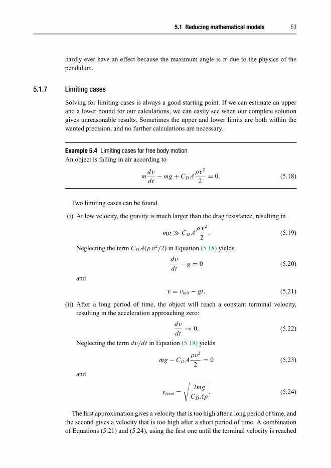
Trim: 247mm × 174mm Top: 12.653mm Gutter: 16.871mmCUUK2531-05 CUUK2531/Rasmuson ISBN: 978 1 107 04969 7 November 13, 2013 16:30
5.1 Reducing mathematical models 63
hardly ever have an effect because the maximum angle is π due to the physics of thependulum.
5.1.7 Limiting cases
Solving for limiting cases is always a good starting point. If we can estimate an upperand a lower bound for our calculations, we can easily see when our complete solutiongives unreasonable results. Sometimes the upper and lower limits are both within thewanted precision, and no further calculations are necessary.
Example 5.4 Limiting cases for free body motionAn object is falling in air according to
mdv
dt− mg + CD A
ρv2
2= 0. (5.18)
Two limiting cases can be found.
(i) At low velocity, the gravity is much larger than the drag resistance, resulting in
mg � CD Aρ v2
2. (5.19)
Neglecting the term CD A(ρ v2/2) in Equation (5.18) yields
dv
dt− g = 0 (5.20)
and
v = vinit − gt. (5.21)
(ii) After a long period of time, the object will reach a constant terminal velocity,resulting in the acceleration approaching zero:
dv
dt→ 0. (5.22)
Neglecting the term dv/dt in Equation (5.18) yields
mg − CD Aρv2
2= 0 (5.23)
and
vterm =√
2mg
CD Aρ. (5.24)
The first approximation gives a velocity that is too high after a long period of time, andthe second gives a velocity that is too high after a short period of time. A combinationof Equations (5.21) and (5.24), using the first one until the terminal velocity is reached

Trim: 247mm × 174mm Top: 12.653mm Gutter: 16.871mmCUUK2531-05 CUUK2531/Rasmuson ISBN: 978 1 107 04969 7 November 13, 2013 16:30
64 Strategies for simplifying mathematical models
Figure 5.4. Velocity of a body falling in air.
and using the terminal velocity after that, will give a good approximation. However, thesolution still overestimates the velocities and the distance the body has fallen, as shownin Figure 5.4.
5.1.8 Neglecting terms
The desired accuracy in prediction is seldom the maximal accuracy that can be obtainednumerically. A good result is if a reactor volume can be estimated to within 10%. Oftenthe calculated reactor volume is increased by 20% to 50% in order to compensate foruncertainties in rate constants and other parameters. In many cases, we can eliminatethe terms in the equations that contribute only a few percent to the final result. If we canestimate whether omitting the terms will give an over- or underestimation of the finalresult, we can compensate for this uncertainty.
5.1.8.1 Order-of-magnitude estimation of derivativesFirst we need some tools for analyzing differential equations. The following method isvery simple and useful, but gives only an order-of-magnitude estimation of the terms in adifferential equation. It is always necessary to verify that the assumptions were justifiedafter the equations have been solved and more accurate estimations of the derivativesare possible.
In a general differential equation, it may be difficult to estimate the influence ofdifferent terms. One approach is to assume a solution and numerically approximate thederivatives. After solving the simplified equation by canceling unimportant terms, theinitial assumptions can be confirmed.
A first-order derivative can be approximated by
dC
dz≈ �C
�z,
and the second-order derivative can be approximated by
d2 C
dz2≈
dC
dz
∣∣∣∣z+dz
− dC
dz
∣∣∣∣z
dz≈
�C
�z
∣∣∣∣L
− �C
�z
∣∣∣∣0
L.

Trim: 247mm × 174mm Top: 12.653mm Gutter: 16.871mmCUUK2531-05 CUUK2531/Rasmuson ISBN: 978 1 107 04969 7 November 13, 2013 16:30
5.1 Reducing mathematical models 65
Figure 5.5. Approximate concentration profiles (solid lines) in the tubular reactor at differentresidence times or rate constants, simulated without the axial dispersion term. The dashed linesindicate slopes of 0.1, 1, and 10, respectively.
Example 5.5 Axial dispersion for a tubular reactionFind a criterion for neglecting the axial dispersion of a first-order reaction in a tubularreactor. A first-order reaction in a tubular reactor without dispersion is described by
Dead 2C
d z2− U
d C
d z− kC = 0. (5.25)
dispersion convection reaction
In the dimensionless form,
1
Pe
d 2C
d z2− d C
d z− kτ C = 0, (5.26)
with τ = L/U , and the boundary conditions
C = 1 at z = 0
and
dC
dz= 0 at z = 1.
First we need an order-of-magnitude estimation of the derivatives. A preliminaryassumption is that the concentration profile has a shape as shown in Figure 5.5, i.e.the outlet concentration is much lower than the inlet concentration, but not zero. Thisassumption must be verified against the final model.
A coarse estimation of the derivatives is for the first-order derivative
dC
dz≈ �C
�z= 0 − C I N
L − 0= −C I N
L, (5.27)

Trim: 247mm × 174mm Top: 12.653mm Gutter: 16.871mmCUUK2531-05 CUUK2531/Rasmuson ISBN: 978 1 107 04969 7 November 13, 2013 16:30
66 Strategies for simplifying mathematical models
in the dimensionless form
dC
dz≈ �C
�z= −1
1= −1; (5.28)
and for the second-order derivative
d2 C
dz2≈
dC
dz
∣∣∣∣z+dz
− dC
dz
∣∣∣∣z
dz≈
�C
�z
∣∣∣∣L
− �C
�z
∣∣∣∣0
L=
0 −(
−CIN
L
)L
= C I N
L2, (5.29)
in the dimensionless form
d2 C
d z2≈
�C
�z
∣∣∣∣∣1
− �C
�z
∣∣∣∣∣0
1= 0 − (−1)
1= 1, (5.30)
using the boundary condition dC/dz = 0 at z = 1.We can now make an order-of-magnitude estimation of the relative importance of the
different terms in (5.26), repeated here for convenience:
1
Pe
d2C
d z2− d C
d z− kCτ = 0
1
Pe1 kτ
The axial dispersion term can be neglected when it is small in comparison with thelargest terms in the model, i.e.
1
Pe� 1 ≈ kτ. (5.31)
It follows from the transport equation (5.26) that kτ ≈ 1 if the axial dispersion canbe neglected. If this criterion is fulfilled, Equation (5.26) can be approximated by
dC
dz= −kCτ. (5.32)
This is a first-order ordinary differential equation. For this type of equation, we needonly one boundary condition. In this case, the inlet condition C = 1 at z = 0 is the mostimportant.
The solution of Equation (5.32) is
C = e−kτ z . (5.33)
An analysis of the validity of the approximations is always necessary, and the first andsecond derivatives are calculated by differentiating Equation (5.33) to obtain
dC
dz= −kτe−kτ z (5.34)
and
d2C
d z2= k2τ 2e−kτ z . (5.35)

Trim: 247mm × 174mm Top: 12.653mm Gutter: 16.871mmCUUK2531-05 CUUK2531/Rasmuson ISBN: 978 1 107 04969 7 November 13, 2013 16:30
5.1 Reducing mathematical models 67
Table 5.1. Conversion, first- and second-order derivatives at the inletand outlet for different residence times
kτ Cout − dC
dz
∣∣∣∣z=0
−dC
dz
∣∣∣∣z=1
d2C
d z2
∣∣∣∣z=0
d2C
d z2
∣∣∣∣z=1
0.69 0.5 0.69 0.35 0.48 0.242.3 0.1 2.3 0.23 5.3 0.534.6 0.01 4.6 0.046 21.2 0.21
The results from the approximative solutions in Equations (5.33)–(5.35) are estimatedfor different parameters kτ in Table 5.1.
The example shows that, for a reactor with a reasonable conversion between 50% and99% (Cout between 0.5 and 0.01), the approximations
− dC
dz
∣∣∣∣∣z=0
≈ 1 andd2C
d z2
∣∣∣∣∣z=0
≈ 1
are within an order of magnitude of the calculated derivatives, except for the second-order derivative at the inlet at high conversion. The criterion that we can neglect axialdispersion when Dea/vL � 1 can, for high conversion, be too weak in some parts ofthe reactor. The criterion
Dea
vL
d2 y
dx2�∣∣∣∣dy
dx
∣∣∣∣ ≈ L
vky,
where the derivatives are calculated from the simplified Equation (5.32), should alwaysbe valid. We also know that (Dea/vL)(d2 y/dx2) > 0, and consequently removing thatterm will result in an overestimation of the conversion.
5.1.9 Changing the boundary conditions
The boundary conditions always affect the solution to an equation, but in many casesthe boundary conditions can be reformulated such that the equation can be solved moreeasily analytically or numerically. In many cases, the boundary conditions are not obviousand have been introduced only to obtain an analytical solution to an equation.
Example 5.6 Boundary condition for a tubular reactor with axial dispersionThis scenario has been discussed for more than 50 years. The condition
dC
dz= 0 at z = L
is under dispute because it introduces a feedback of information from the end of thereactor that does not occur in real reactors. A more realistic formulation for anirreversible reaction is perhaps
C → 0 when x → ∞.

Trim: 247mm × 174mm Top: 12.653mm Gutter: 16.871mmCUUK2531-05 CUUK2531/Rasmuson ISBN: 978 1 107 04969 7 November 13, 2013 16:30
68 Strategies for simplifying mathematical models
For diffusion and reaction in a porous spherical catalyst, the condition
dC
dr= 0 at r = 0
is not necessary. A boundary condition that does not allow diffusive transport throughthe center of the catalyst may be sufficient, i.e.
r2 dC
dr→ 0 when r → 0,
and a sufficient condition is that the derivative dC/dr is limited when r → 0. In addition,the condition C = 0 at a distance δ from the surface could even be appropriate for fastreactions.
5.2 Case study: Modeling flow, heat, and reaction in a tubular reactor
The methods listed in Sections 5.1.1–5.1.7 are illustrated by a tubular reactor with afirst-order reaction and laminar flow. Models for species, heat, and momentum havebeen formulated and simplified. In addition to showing the methods, we discuss theassumptions in a traditional 1D lumped-parameter model for a tubular reactor with axialdispersion,
∂C
∂t= Dea
∂2C
∂z2− v
∂C
∂z− kn(T, t) · Cn, (5.36)
ρmcm∂T
∂t= λea
∂2T
∂z2− vρcp
∂T
∂z− kn(T, t)(−�H ) · Cn. (5.37)
5.2.1 General equation for a cylindrical reactor
The following equations describe transport of species, heat, and momentum in a cylin-drical tubular reactor with laminar flow
Material balance for species A
∂ CA
∂ t+ vz
∂ CA
∂ z+ vr
∂ CA
∂ r+ vθ
r
∂ CA
∂ θ
= DA
[1
r
∂
∂ r
(r∂ CA
∂ r
)+ ∂2 CA
∂ z2+ 1
r2
∂2CA
∂θ2
]− RA (5.38)
Heat balance
ρcP
(∂ T
∂ t+ vz
∂ T
∂ z+ vr
∂ T
∂ r+ vθ
r
∂ T
∂ θ
)
= k
[1
r
∂
∂ r
(r∂ T
∂ r
)+ ∂2 T
∂ z2+ 1
r2
∂2T
∂θ2
]+ Q A. (5.39)

Trim: 247mm × 174mm Top: 12.653mm Gutter: 16.871mmCUUK2531-05 CUUK2531/Rasmuson ISBN: 978 1 107 04969 7 November 13, 2013 16:30
5.2 Case study: Modeling flow, heat, and reaction in a tubular reactor 69
Balances for axial, z, radial, r, and tangential, θ , momentum
ρ
(∂ vz
∂ t+ vr
∂ vz
∂ r+ vz
∂ vz
∂ z+ vθ
r
∂ vz
∂ θ
)= μ
[1
r
∂
∂ r
(r∂ vz
∂ r
)+ ∂2 vz
∂ z2+ 1
r2
∂2vz
∂θ2
]
+ ρ Gz − ∂ p
∂ z; (5.40)
ρ
(∂ vr
∂ t+ vr
∂ vr
∂ r+ vz
∂ vr
∂ z+ vθ
r
∂ vr
∂ θ− v2
θ
r
)
= μ
[∂
∂ r
(1
r
∂
∂ r(rvr )
)+ ∂2 vr
∂ z2+ 1
r2
∂2vz
∂θ2− 2
r
∂vz
∂θ
]+ ρ Gr − ∂ p
∂ r; (5.41)
ρ
(∂ vθ
∂ t+ vr
∂ vθ
∂ r+ vz
∂ vθ
∂ z+ vθ
r
∂ vθ
∂ θ− vrvθ
r
)
= μ
[∂
∂ r
(1
r
∂
∂ r(rvθ )
)+ ∂2 vθ
∂ z2+ 1
r2
∂2vz
∂θ2+ 2
r
∂vz
∂θ
]+ ρ Gθ − 1
r
∂ p
∂ θ. (5.42)
Equation of continuity
∂ρ
∂ t+ 1
r
∂
∂ r(ρ r vr ) + 1
r
∂
∂θ(ρvθ ) + ∂
∂ z(ρ vz) = 0. (5.43)
5.2.1.1 Boundary conditionsAt the inlet, we have only axial velocity, and no radial or tangential variation in concen-tration or temperature:
vZ = vav, vr = 0, vθ = 0, C = C I N , T = T I N .
At the outlet, we have only axial velocity and axial convection of species and heat:
vr = 0, vθ = 0,∂vZ
∂z= 0,
∂C
∂z= 0,
∂T
∂z= 0.
We have no slip at the wall and no penetration of species, but heat transfer though thewall will occur:
vZ = 0, vr = 0, vθ = 0,∂C
∂r= 0, k
∂T
∂r= u(T − TW ).
The boundary conditions are not obvious; they require detailed knowledge of theactual flow pattern, and, as discussed, the outlet conditions are questionable.
5.2.2 Reducing the number of independent variables
With no density differences in the fluid, there will be no source term for the radial andtangential velocities. If the inlet and boundary conditions are axisymmetric, there willbe no variation in the θ direction. Removing the tangential variations will allow us toreduce the simulation from 3D to 2D. The symmetric boundary condition at the centerof the tube can be formulated as
∂vr
∂r= 0,
∂vz
∂r= 0,
∂C
∂r= 0,
∂T
∂r= 0 at r = 0.

Trim: 247mm × 174mm Top: 12.653mm Gutter: 16.871mmCUUK2531-05 CUUK2531/Rasmuson ISBN: 978 1 107 04969 7 November 13, 2013 16:30
70 Strategies for simplifying mathematical models
With no variation in tangential direction, the balance equation for tangential momen-tum, Equation (5.42), and the θ dependence in the remaining Equations (5.38)–(5.43)should be removed.
Radial velocity will occur due to the inlet velocity, which has not taken the finalparabolic form. A general rule of thumb is that the variation in radial velocity that arisesfrom an uneven inlet can be neglected in a pipe after an inlet distance of δ, estimatedfrom the pipe diameter and the Reynolds number:
δ
d= 0.05 Re.
5.2.3 Steady state or transient?
How fast the concentration or temperature will change due to a step change at an inletgives us an idea about the time resolution that is required for a transient solution, andhow quickly the reactor will reach steady state. One way to retrieve the time constantsis to compare the accumulation term with the dominating transport term.
Axial transport: the ratio of accumulation to convection is written and simplified as
∂ CA/∂t
vz(∂ CA/∂z)≈ �CA/�t
vZ (�CA/�z)≈ CA,inτ
vz(CA,in/L).
This gives the time constant for axial convection as
τ = CA,in
vz CA,in/L= L
vz.
Radial diffusion
∂ CA/∂t
D1
r
∂
∂r
(r∂ CA
∂r
) ≈ �CA/�t
D1
R
(R
�C
�r2
) ≈ CA/τ
DCA/R2.
This gives the time constant for radial diffusion as
τ = CA/(DCA/R2) = R2
D.
As expected, it will take one residence time L�vz for a change in inlet concentrationto affect the whole length of the reactor, and it will take R2�D for the concentration todiffuse from the center of the reactor to the wall in accordance with the time constantsdeveloped in Section 5.1.5.
Similar time constants can be estimated for momentum and heat transfer also.Table 5.2 shows the time constants for convective transport in the axial direction, theradial transport of momentum, mass, and heat, assuming L = 10 m, v = 0.1 m s−1
and laminar flow. The fluid properties that are typical for a gas are: density 1 kg m−3,diffusivity 10−5 m2 s−1, heat capacity 1000 J kg−1 K−1. Typical liquid properties are:density 1000 kg m−3, diffusivity 10−9 m2 s−1, heat capacity 1000 J kg−1 K−1, heatconductivity 0.5 W m−2 K−1. The main differences between gases and liquids are in the

Trim: 247mm × 174mm Top: 12.653mm Gutter: 16.871mmCUUK2531-05 CUUK2531/Rasmuson ISBN: 978 1 107 04969 7 November 13, 2013 16:30
5.2 Case study: Modeling flow, heat, and reaction in a tubular reactor 71
Table 5.2. Time constants of a 0.1 m/s gas and liquid flow in a 10 m tubular reactor with two differenttube diameters, R
The fluid properties are typical for gas and liquid
Conditions
Axialtransport,L/vz
Radialmomentum,R2ρ/μ
Radialdiffusion,R2/D
Radial heatconduction,R2ρcp/k
Air (25 °C, 1 bar, R = 0.1 m) 100 500 1000 400Water (25 °C, R = 0.005 m) 100 100 25 000 200
diffusivity and heat conduction. The very low diffusivity in liquids is, to some extent,compensated for in the table by a much smaller tube radius.
With a step response at the inlet and no external time-dependent influence, the reactorwill reach steady state after the largest of the time constants. The much larger timeconstants for the radial diffusion (R2�D) than for the residence time (L�v), indicate thatthe concentration will vary radially within the whole reactor if the inflow does not haveequal concentration over the cross section.
In this case study we assume a constant even flow and concentration at the inletand only consider steady state. However, the concentration will have a radial variationdownstream due to the reaction and the radial difference in residence time. Assumingan even inflow and a minor effect of gravity in the radial and tangential directions, theconvective radial transport terms can be removed. Axial viscous transport, diffusion,and conduction can also be neglected because the convective axial transport is muchlarger. After a sufficiently long period of time, the transient terms become very small,and we obtain a model with steady axial convection, radial diffusion, and conductionwith a reaction source term.
Material balance
vz∂ CA
∂z= D
1
r
∂
∂r
(r∂ CA
∂r
)− RA. (5.44)
Heat balance
ρcp
(vz
∂ T
∂ z
)= k
1
r
∂
∂ r
(r∂ T
∂ r
)+ QA. (5.45)
Momentum balance
ρ
(vz
∂ vz
∂ z
)= μ
1
r
∂
∂ r
(r∂ vz
∂ r
)+ ρ Gz − ∂ p
∂ z. (5.46)
Equation of continuity
∂
∂ z(ρ vz) = 0. (5.47)

Trim: 247mm × 174mm Top: 12.653mm Gutter: 16.871mmCUUK2531-05 CUUK2531/Rasmuson ISBN: 978 1 107 04969 7 November 13, 2013 16:30
72 Strategies for simplifying mathematical models
5.2.4 Decoupling equations
If, in the case study, μ and ρ are assumed to be independent of CA and T in theactual concentration and temperature interval, the solution of the equations is drasticallysimplified. The equation of continuity gives ∂vz/∂ z = 0, and using this in Equation(5.46) yields
μ1
r
∂
∂r
(r
∂vz
∂r
)= ∂p
∂z− ρ Gz = constant. (5.48)
Integrating Equation (5.48) and using ∂vz/∂ r = 0 when r = 0 and vz = 0 when r =R yields
vz(r ) =(
ρ Gz − ∂p
∂z
)R2
4μ
(1 − r2
R2
)= 2 vav
(1 − r2
R2
), (5.49)
where vav denotes the average velocity in the pipe. As expected, we obtain the parabolicvelocity profile for laminar flow in a circular pipe.
5.2.5 Simplified geometry
We have now reduced the equations to two coupled partial differential equations (usingEquation (5.49) in Equations (5.44) and (5.45):
2 vav
(1 − r2
R2
)∂ CA
∂z= D
1
r
∂
∂ r
(r
∂ CA
∂ r
)− RA; (5.50)
ρ cP 2 vav
(1 − r2
R2
)∂ T
∂z= k
1
r
∂
∂ r
(r
∂ T
∂ r
)+ Q A. (5.51)
The dimensionless space coordinates r = r/R and z = z/L yield
2(1 − r2
) ∂ CA
∂ z= L D
R2 vav
1
r
∂
∂ r
(r
∂ CA
∂ r
)− L
vav
· RA; (5.52)
2(1 − r2
) ∂ T
∂ z= L · k
R2 vavρ cp
1
r
∂
∂ r
(r
∂ T
∂ r
)+ L
vav ρ cp· QA. (5.53)
In order to obtain ordinary differential equations, we must eliminate one space coor-dinate. There are several possibilities for doing this: we can calculate an average byintegrating over the radial or axial coordinates; we can find simple polynomials that canapproximate the radial concentration and temperature dependencies; or we can assumethat the radial coupling is negligible.
The simplest solution is to use the radial average, as we assume that the axial variationsare larger than the radial variations.
First, we integrate radially (this mean to integrate over a thin circular slice 2πr dr,which in the dimensionless form is 2π r dr ). The integration of the radial transport term

Trim: 247mm × 174mm Top: 12.653mm Gutter: 16.871mmCUUK2531-05 CUUK2531/Rasmuson ISBN: 978 1 107 04969 7 November 13, 2013 16:30
5.2 Case study: Modeling flow, heat, and reaction in a tubular reactor 73
is straightforward because
1∫0
d
dr
(r
dy
dr
)dr = r
dy
dr
∣∣∣∣r=1
−rdy
dr
∣∣∣∣r=0
= rdy
dr
∣∣∣∣r=1
and
1∫0
2(1 − r2
) ∂ CA
∂ z2π r dr = 2π
L D
R2 vav
∂ cA
∂ r
∣∣∣∣r=1
−1∫
0
L
vav
RA 2π r dr , (5.54)
1∫0
2(1 − r2
) ∂ T
∂ z2π r dr = 2π
L k
R2 vav ρ cp
∂ T
∂ r
∣∣∣∣r=1
+1∫
0
L
vav ρ cpQA 2π r dr . (5.55)
The wall is not permeable for mass transport, i.e.
∂CA
∂ r
∣∣∣∣r=1
= 0. (5.56)
Heat is conducted through the wall, so
k∂T
∂r
∣∣∣∣r=R
= k
R
∂T
∂ r
∣∣∣∣r=1
= u(Tw − Tx=1). (5.57)
We define the mixed-cup average CA using
CA · vav =
1∫0
2vav( 1 − r2) CA (z, r ) 2π r dr
1∫0
2π r dr
=1∫
0
2vav
(1 − r2
)CA (z, r ) 2r dr (5.58)
and the mixed-cup average T using
T vav =1∫
0
2 vav
(1 − r2
)T (z, r ) 2r dr . (5.59)
Observe that this averaging over the radius also eliminates the axial dispersion that iscaused by the parabolic velocity profile.

Trim: 247mm × 174mm Top: 12.653mm Gutter: 16.871mmCUUK2531-05 CUUK2531/Rasmuson ISBN: 978 1 107 04969 7 November 13, 2013 16:30
74 Strategies for simplifying mathematical models
Also note that the difference between the mixed-cup average and the average 〈C〉
〈CA〉 =
1∫0
CA (z, r ) 2π r dr
1∫0
2π rdr
=1∫
0
CA (z, r ) 2r dr (5.60)
over the cylinder, is due to the radial variation in velocity. If we take a sample from theoutlet to measure concentration, we will obtain more sample from the center of the pipedue to the higher velocity in the center. If we measure concentration spectrometrically,we will have equal contribution from all parts, irrespective of velocity. Usually it is themixed-cup average we need as it is related to the total amount converted in the reactor.
The final integrals on the right-hand side of Equations (5.54) and (5.55) are approxi-mated by
2
1∫0
L
vav
RA (CA, T ) r dr ≈ L
vav
RA (CA, T ), (5.61)
2
1∫0
L
vavρ cpQA r dr ≈ L
vav ρ cpQA (cA, T ), (5.62)
i.e. the average of the reaction rate is approximated by the reaction rate at averagedconcentration and temperature.
We now have two coupled ordinary differential equations:
dC
dz= − L
vav
RA (CA, T ), (5.63)
dT
dz= 2
Lu
R vavρ cp(Tw − T ) + L
vav ρ cpQA (CA, T ). (5.64)
However, comparing the heat flux through the wall, we have
u(TW − Tx=1) = u(TW − T ), (5.65)
but, because the mixed-cup temperature differs from the wall temperature, i.e.
T �= Tr=1,
we must adjust u; one common method is to add a part of the heat transfer resistance inthe reactor as follows:
1
u= 1
u+ α
r
k. (5.66)
By making this adjustment we assume that we have the temperature T , a distance αRfrom the wall, and that heat is conducted through the fluid and the wall.
Because the equations are non-linear, there is still no analytical solution to the equa-tions. The equations describe a simple initial value problem, and numerical solutions arestraightforward. An analytical solution is possible only if we assume that, by efficient

Trim: 247mm × 174mm Top: 12.653mm Gutter: 16.871mmCUUK2531-05 CUUK2531/Rasmuson ISBN: 978 1 107 04969 7 November 13, 2013 16:30
5.2 Case study: Modeling flow, heat, and reaction in a tubular reactor 75
cooling or through a reaction of low heat of reaction, the temperature will be constantaxially and the reaction rate will be a function of concentration only, i.e.
∫ CU TA
C I NA
dCL
vav
RA (CA)= −
1∫0
dz. (5.67)
5.2.6 Limiting cases
The partial differential equation, Equation (5.52), can be approximated by using differentassumptions. For an isothermal case, it can be written, for a first-order reaction, asfollows:
2 (1 − r2)∂ C
∂ z= DL
R2vav
1
r
∂
∂ rr
∂ C
∂ x− L k1
vav
C. (5.68)
(1) Assuming no radial variations. When the residence time is much larger than the timefor radial diffusion, i.e.
L
vav
� R2
D, (5.69)
the ratio between residence time and the radial diffusion time constant appears inthe term for radial diffusion, and
DL
R2 vav
→ ∞
⇒ ∂ C
∂ r→ 0
⇒ C(r , z) = C(z);
i.e. the radial concentration is assumed to be constant, equal to the mixed-cupaverage, as shown by eliminating radial variation. Integrating the average flow,
1∫0
2(1 − r2
) ∂C
∂ z2r dr = ∂C
∂ z, (5.70)
will simplify the model to
dC
d z= − L k1
vav
C, (5.71)
C = exp[−(Lk/vav)z]. (5.72)
(2) Assuming no radial transport, i.e. a very short residence time in comparison to thetime for radial diffusion, i.e.
R2
D� L
vav
,
will remove the radial diffusion term and Equation (5.68) will be simplified to
2 (1 − r2)∂ C
∂ z= − Lk1
vav
· C. (5.73)

Trim: 247mm × 174mm Top: 12.653mm Gutter: 16.871mmCUUK2531-05 CUUK2531/Rasmuson ISBN: 978 1 107 04969 7 November 13, 2013 16:30
76 Strategies for simplifying mathematical models
Rearranging this equation yields
∂ C
C= − L k1
2 · vav(1 − r2)∂ z (5.74)
and the solution
C (z, r ) = Cin exp
[− L · k1
2 · vav(1 − r2)· z
](5.75)
The concentration in the outlet will be a function of both radius and reactorlength. A mixed-cup average is obtained by integrating the concentration accordingto Equation (5.58).
5.2.7 Conclusions
The complex partial differential equations have been simplified all the way, until ananalytical solution is possible. The simplifications can be halted at any point dependingon the desired accuracy and available numerical tools.
The assumptions in a lumped-parameter model are not always transparent. For exam-ple, in the 1D model for a tubular reactor with axial dispersion (Equations (5.36) and(5.37), repeated here for convenience)
∂C
∂t= Dea
∂2C
∂z2− v
∂C
∂z− kn(T, t) · Cn,
ρcp∂T
∂t= λea
∂2T
∂z2− vρcp
∂T
∂z− kn(T, t)(−�H ) · Cn, (5.37)
where the axial dispersion term Dea can be estimated from
Dea = D + R2v2
192D,
and λea by replacing D by heat conduction k in the equation.The main assumptions in the lumped parameter model are
(1) the average reaction rate is the rate at average temperature and concentration;(2) the axial dispersion term describes the complex combination of transport by velocity
gradients and diffusion;(3) the velocity is the traditional average, and the concentration and temperature are the
mixed-cup averages.
5.3 Error estimations
The simulations must be validated and verified before they can be trusted. At thebeginning of this chapter, we stated that poor simulation results may be due to manydifferent reasons: errors in formulating the problem, inaccurate models, inaccurate dataon physical properties, numerical errors due to the choice of numerical methods, andlack of convergence in the simulations.

Trim: 247mm × 174mm Top: 12.653mm Gutter: 16.871mmCUUK2531-05 CUUK2531/Rasmuson ISBN: 978 1 107 04969 7 November 13, 2013 16:30
5.4 Questions 77
5.3.1 Sensitivity analysis
Validating the model by comparing it with the experimental data of a similar systemis the most direct way to test all the aforementioned errors. However, it is not alwaysobvious what a difference between simulations and experiments indicates, and it isimportant to try to evaluate each possible error separately. Errors in formulating theproblem may be recognized from simulations of limiting cases, e.g. very high or lowkinetic rate constants or velocities. Simulation of an isothermal case will remove errorsin the heat balance, and simulation using a preset velocity profile will remove errorsin the momentum balance, etc. Inaccurate physical data can be evaluated by making asmall change in data values and estimating how sensitive the results are to the absolutevalue of the variables. This type of analysis will tell us which variables are critical andmust be known very accurately.
In addition to changing parameters to determine the influence of different phenomena,the influence of the different terms in a model can be estimated by putting a weightingfactor in front of each term in the model, e.g. the accumulation term or the axialdispersion term in a chemical reactor model, and comparing the simulations. In thisway, we can easily estimate which factors dominate the model, and perhaps remove theparts that have negligible influence. We can also judge whether the result supports ourexpectations or whether the model must be reformulated.
Numerical errors and convergence can be tested by changing the initial guess of thesolution and the numerical accuracy in the numerical subroutines. In an optimization orleast-squares minimization using a gradient search, it is important to have high accuracyin order to calculate a correct gradient. The step length in a gradient evaluation mustbe chosen sufficiently large in comparison with the solution accuracy. A gradient-freesearch, e.g. a random Monte Carlo method, may be more efficient.
5.3.2 Over- and underestimations
A sensitivity analysis will reveal how variables affect final results. We can find out, e.g.,whether our estimated chemical reactor volume will increase or decrease when a certainparameter is increased. If that parameter is uncertain, we can simulate for an upper anda lower value of that parameter and obtain an over- and an underestimation of, e.g., thereactor volume. The same method can be used for other uncertainties in modeling, e.g.to compare results assuming laminar or turbulent flow, and whether to include radiationor not.
5.4 Questions
(1) What properties are essential in an equation that may be solved independently of theremaining equations in a system of equations?
(2) Why are the net mass and heat transfer through a symmetry boundary conditionzero?
(3) What are the maximum number of symmetry planes in a cube, cylinder, and sphere?
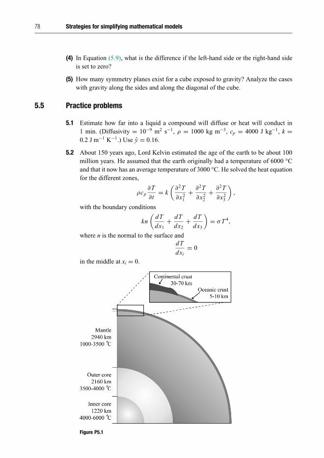
Trim: 247mm × 174mm Top: 12.653mm Gutter: 16.871mmCUUK2531-05 CUUK2531/Rasmuson ISBN: 978 1 107 04969 7 November 13, 2013 16:30
78 Strategies for simplifying mathematical models
(4) In Equation (5.9), what is the difference if the left-hand side or the right-hand sideis set to zero?
(5) How many symmetry planes exist for a cube exposed to gravity? Analyze the caseswith gravity along the sides and along the diagonal of the cube.
5.5 Practice problems
5.1 Estimate how far into a liquid a compound will diffuse or heat will conduct in1 min. (Diffusivity = 10−9 m2 s−1, ρ = 1000 kg m−3, cp = 4000 J kg−1, k =0.2 J m−1 K−1.) Use y = 0.16.
5.2 About 150 years ago, Lord Kelvin estimated the age of the earth to be about 100million years. He assumed that the earth originally had a temperature of 6000 °Cand that it now has an average temperature of 3000 °C. He solved the heat equationfor the different zones,
ρcp∂T
∂t= k
(∂2T
∂x21
+ ∂2T
∂x22
+ ∂2T
∂x23
),
with the boundary conditions
kn
(dT
dx1+ dT
dx2+ dT
dx3
)= σ T 4,
where n is the normal to the surface anddT
dxi= 0
in the middle at xi = 0.
Figure P5.1

Trim: 247mm × 174mm Top: 12.653mm Gutter: 16.871mmCUUK2531-05 CUUK2531/Rasmuson ISBN: 978 1 107 04969 7 November 13, 2013 16:30
5.5 Practice problems 79
Discuss how the following methods can be used to simplify the calculations:� decoupling of equations;� reducing the number of independent variables;� separation of equations into steady state and transient;� simplifying geometry;� linearizing;� neglecting terms;� solving for limiting cases.
Make your own estimation using the data in Figure P5.1. The radiation inflowfrom the sun and the radiation outflow are today the dominant terms; the solarconstant is 1400 W m−2. The net flux from the inner part of the earth is today onthe order of 5 · 10−2 W m−2. Assume a heat capactity of 5 · 106 J m−3 K−1.
5.3 Most of the harmful emissions from cars appear during cold start because thecatalyst has to reach 250 °C before it becomes active. It takes about 1 min undernormal driving conditions. An opening to reduce the time is to put a smaller catalystwith less thermal mass close to the engine. Using late ignition in the engine makesit possible to raise the exhaust temperature very quickly. Calculate Do an over- andunderestimation of how long it will take to heat the catalytic converter to 250 °Cwhen the exhaust gas temperature increases linearly from 20 to 700 °C for 10 s andthen kept constant.
The catalyst has a volume of 0.5 l and a mass of 100 g. The channel surface(i.e. the area of contact with the exhaust gases) is 2000 m2 m−3. The mass flowof the exhaust gas is 0.01 kg s−1. Assume that the catalyst heat capacity is 1000 Jkg−1 K−1, and of the exhaust gas is 1000 J kg−1 K−1. The Nusselt number for heattransfer in the channels is 4, and the gas heat conduction is 0.04 W K−1 m−1.
5.4 Over 80 times more CO2 is dissolved in the sea than in the atmosphere, and thegas will not contribute to global warming if it dissolves in the oceans. The primarymechanism for the transport of CO2 from the atmosphere to the ocean is throughits dissolution in raindrops. Calculate approximate (over- and underestimates) howmuch it needs to rain in Sweden (486 000 km2) in m m−2 if the production ofCO2 (55 million tons y−1) is balanced with the amount that dissolves in the rain.Assume that the raindrops are of about 6 mm diameter and that they fall with avelocity of 10 m s−1 from 1000 m.
The transport of the CO2 into a raindrop can be approximated by diffusion:
∂C
∂t= D
(∂2C
∂r2+ 2
r
∂C
∂r
).
The atmospheric CO2 concentration is 0.0325%, and its solubility in water is 40 molm−3, bar−1. The diffusivity of CO2 in water is 10−9 m2 s−1. The model neglects thedeformation of the droplet, the convection inside the droplet, and the mass transferin the air outside the droplet. Does this lead to an over- or underestimation of CO2
transport into the drop?Hint: Estimate how far into the drop the CO2 can diffuse in the available time.

Trim: 247mm × 174mm Top: 12.653mm Gutter: 16.871mmCUUK2531-05 CUUK2531/Rasmuson ISBN: 978 1 107 04969 7 November 13, 2013 16:30
80 Strategies for simplifying mathematical models
5.5 The surface temperature in the desert can vary between +80 °C during day-time and −10 °C during the night. Estimate how far into the sand the tempera-ture fluctuations can reach. Define the position where no fluctuation is observedas the point where less than 1% of the surface variations are noticed. The densityof the sand is 2000 kg m−3, the heat conductivity is 0.8 W m−1 K−1, and the heatcapacity is 1000 J kg−1 K−1.
5.6 Monolithic catalytic converters with a large number of parallel channels are verycommon in emission control for cars. The flow is laminar in order to minimizepressure drop with parabolic velocity profile. The maximum velocity in the centeris twice the average velocity. Calculate the required catalyst volume assumingthe rate-determining step is that the pollutants should have time to diffuse fromthe center of the channel to the catalytic wall. The channels are 1 mm wide and thechannel volume is 80% of the catalytic converter volume. The volumetric flow ofexhaust gas for a 2 l engine running at 3000 rpm can be approximated as (enginespeed) × (engine volume)/2.

Trim: 247mm × 174mm Top: 12.653mm Gutter: 16.871mmCUUK2531-06 CUUK2531/Rasmuson ISBN: 978 1 107 04969 7 November 13, 2013 17:2
6 Numerical methods
Differential equations play a dominant role in mathematical modeling. In practical engi-neering applications, only a very limited number of them can be solved analytically.The purpose of this chapter is to give an introduction to the numerical methods neededto solve differential equations, and to explain how solution accuracy can be controlledand how stability can be ensured by selecting the appropriate methods. The mathe-matical framework needed to solve both ordinary and partial differential equations ispresented. A guideline for selecting numerical methods is presented at the end of thechapter.
6.1 Ordinary differential equations
A characteristic of a differential equation is that it involves an unknown function andone or more of the function’s derivatives. If the unknown function depends on onlyone independent variable, it is classified as an ordinary differential equation (ODE). Theorder of the differential equation is simply the order of the highest derivative that appearsin the equations. Consequently, a first-order ODE contains only first derivatives, whilsta second-order ODE may contain both second and first derivatives. The ODEs can alsobe classified as linear or non-linear. Linear ODEs are the ones in which all dependentvariables and their derivatives appear in a linear form. This implies that they cannot bemultiplied or divided by each other, and they must be raised to the power of 1. An ODEhas an infinite number of solutions, but with the appropriate conditions that describesystems, i.e. the initial value or the boundary value, the solutions can be determineduniquely.
6.1.1 ODE classification
ODEs can be classified as initial-value problems (IVPs), or boundary-value problems(BVPs). The classification into IVP or BVP depends on the location of the extra condi-tions specified. For IVPs they are given at the same value of the independent variable (thelower boundary, and consequently the initial value), whereas for BVPs they are givenat different values of the independent variable. Consider Equation (6.1), a second-order

Trim: 247mm × 174mm Top: 12.653mm Gutter: 16.871mmCUUK2531-06 CUUK2531/Rasmuson ISBN: 978 1 107 04969 7 November 13, 2013 17:2
82 Numerical methods
ODE on an interval x ∈ [a, b], with two different sets of conditions, which cause theequation to be classsified as either IVP or BVP:
d2 y
dx2= f
(x, y,
dy
dx
). (6.1)
Initial-value problem
y(a) = α,
dy
dx
∣∣∣∣x=a
= β.
Boundary-value problem
y(a) = α,
y(b) = γ.
The numerical methods used to solve these two classes of problems, i.e. IVPs andBVPs, are different, and the two separate conditions for the BVP generally make it moredifficult to solve. Methods for solving both of these types of problems will be introducedin this chapter.
6.1.2 Solving initial-value problems
In order to give an introduction to the most important concepts used in different methods,such as accuracy, stability, and efficiency, we will start with the explicit Euler method,which is the simplest numerical method to use when solving ODEs. At this point, weshould stress that the accuracy of this method is low, and that it is only conditionallystable. For this reason, it is not used in practice to solve any engineering problems.However, it serves well to illustrate a method for solving ODEs numerically, and forintroducing the concepts of accuracy and stability. Later in this chapter more advancednumerical methods will be presented; methods that have higher accuracy and betterstability properties, and that are implemented in modern software products.
6.1.2.1 The explicit Euler methodConsider the solution of an initial-value problem
dy
dx= f (x, y), (6.2)
with the initial condition y(x0) = y0. The approach used in the explicit Euler method isbased on the discretization of the interval x ∈ [a, b] into M equal subintervals, whichgives the step size h = (b − a) �M. The explicit Euler method approximates the solutionas
yn+1 = yn + h f (xn, yn). (6.3)

Trim: 247mm × 174mm Top: 12.653mm Gutter: 16.871mmCUUK2531-06 CUUK2531/Rasmuson ISBN: 978 1 107 04969 7 November 13, 2013 17:2
6.1 Ordinary differential equations 83
Figure 6.1. Principle of the Euler method.
The error made in the Euler method in a single step, ε, can be estimated by using theTaylor expansion
y(x0 + h) = y(x0) + hy′(x0) + 1
2h2 y′′(x0) + O(h3). (6.4)
By subtracting Equation (6.3) from Equation (6.4) we obtain
ε = 1
2h2 y′′(x0) + O(h3), (6.5)
which shows that the local truncation error is approximately proportional to h2. It canalso be shown that the global error over the interval x ∈ [a, b] is O(h). (This will bedicussed in detail later in the chapter.) As shown in Figure 6.1, the derivative changesbetween xn and xn+1, but the Euler method simply relies on the derivative at xn.
Example 6.1 Error versus step sizeA simple problem illustrates how the error is related to step size. Consider thefollowing problem: ⎧⎪⎪⎨
⎪⎪⎩dy
dt= f (t, y) = y + t,
y(0) = 1,
t ∈ [0, 1].
The numerical solution using the explicit first-order Euler method, and the step sizeh = 0.2, is shown in Figure 6.2.
By using the globally first-order accurate Euler method, O(h), the error is halvedbecomes when the step size is halved. If the step size is further reduced, the global errorcontinues to decrease, but very slowly, as shown in Figure 6.3. A major drawback of theEuler method is that it has low accuracy; a very small step size is required to control andkeep error low. The errors, shown in Figure 6.3, have been calculated as the difference

Trim: 247mm × 174mm Top: 12.653mm Gutter: 16.871mmCUUK2531-06 CUUK2531/Rasmuson ISBN: 978 1 107 04969 7 November 13, 2013 17:2
84 Numerical methods
Figure 6.2. Solution using the Euler method, step size h = 0.2.
Figure 6.3. Global error vs. step size.
between the numerical solution and the true value. In this case, the error can be easilycalculated as the analytical solution is given by y(t) = 2 exp(t) − t − 1.
6.1.2.2 The midpoint methodThe midpoint method is an improvement on the Euler method in that it uses informationabout the function at a point other than the initial point of the interval. As seen inFigure 6.4, the values of x and y at the midpoint are used to calculate the step across thewhole interval, h.

Trim: 247mm × 174mm Top: 12.653mm Gutter: 16.871mmCUUK2531-06 CUUK2531/Rasmuson ISBN: 978 1 107 04969 7 November 13, 2013 17:2
6.1 Ordinary differential equations 85
Figure 6.4. Principle of the midpoint second-order Runge–Kutta method.
Figure 6.5. Solution using the midpoint method, step size h = 0.2.
The midpoint method requires two function evaluations in the step,
k1 = h f (xn, yn), (6.6)
k2 = h f (xn + h/2, yn + k1/2), (6.7)
and gives the approximate solution as
yn+1 = yn + k2 + O(h3). (6.8)
Consequently, the midpoint method increases accuracy by one order. Obviously theincreased order of accuracy leads to a better approximation than the Euler solution, asshown in Figure 6.5.
A comparison between the errors in the Euler and midpoint methods is summarizedin Table 6.1 and shown in Figure 6.6.
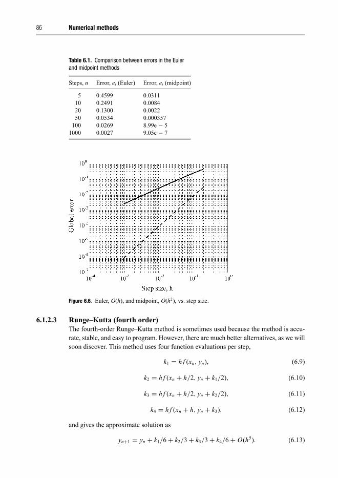
Trim: 247mm × 174mm Top: 12.653mm Gutter: 16.871mmCUUK2531-06 CUUK2531/Rasmuson ISBN: 978 1 107 04969 7 November 13, 2013 17:2
86 Numerical methods
Table 6.1. Comparison between errors in the Eulerand midpoint methods
Steps, n Error, ei (Euler) Error, ei (midpoint)
5 0.4599 0.031110 0.2491 0.008420 0.1300 0.002250 0.0534 0.000357
100 0.0269 8.99e − 51000 0.0027 9.05e − 7
Figure 6.6. Euler, O(h), and midpoint, O(h2), vs. step size.
6.1.2.3 Runge–Kutta (fourth order)The fourth-order Runge–Kutta method is sometimes used because the method is accu-rate, stable, and easy to program. However, there are much better alternatives, as we willsoon discover. This method uses four function evaluations per step,
k1 = h f (xn, yn), (6.9)
k2 = h f (xn + h/2, yn + k1/2), (6.10)
k3 = h f (xn + h/2, yn + k2/2), (6.11)
k4 = h f (xn + h, yn + k3), (6.12)
and gives the approximate solution as
yn+1 = yn + k1/6 + k2/3 + k3/3 + k4/6 + O(h5). (6.13)

Trim: 247mm × 174mm Top: 12.653mm Gutter: 16.871mmCUUK2531-06 CUUK2531/Rasmuson ISBN: 978 1 107 04969 7 November 13, 2013 17:2
6.1 Ordinary differential equations 87
Figure 6.7. Local and global errors.
These methods (Euler, midpoint, and Runge–Kutta) are examples of explicit algorithms.For the same step size, the higher-order Runge–Kutta method gives better precision butat the cost of more calculations in each step.
6.1.3 Numerical accuracy
There are always errors present when we solve differential equations numerically. Theseerrors can be divided into two different parts:
� a local truncation error, which is due to the numerical method in each step;� a global error, which is due to previous local errors and amplification.
To be clear, let us first define the correct solution to the initial-value problem as y(x).The approximative solution using a single-step numerical method, e.g. the Euler method,with an increment function f (xn, yn) and step size h is yn+1 = yn + h f (xn, yn), and itis approximated at a number of discrete points {(xn, yn)}M
n=0.The global truncation error, en, is defined as the difference between the ODE solver
approximation, yn , and the correct solution of the IVP, y(xn):
en = yn − y(xn). (6.14)
The local error, εn+1, is defined as the error committed in each step from xn to xn+1.Let us introduce z(x), which is the correct solution of the IVP over that single step. Thelocal truncation error is then given by
εn+1 = yn+1 − z(xn+1). (6.15)
Whereas the local error is due to a single step, the global error, en+1, is the sum of thelocal error, εn+1, and the amplified error from previous steps. As a consequence, it isnot equal to the sum of the local errors from previous steps. The local and global errorsare illustrated in Figure 6.7. Note that the upper curve, y(x), is the correct (true) solutionto the IVP and that the lower curve, z(x), is the correct solution of the IVP on xn < x <
xn+1, given y(xn) = yn.

Trim: 247mm × 174mm Top: 12.653mm Gutter: 16.871mmCUUK2531-06 CUUK2531/Rasmuson ISBN: 978 1 107 04969 7 November 13, 2013 17:2
88 Numerical methods
Table 6.2. Summary of accuracy of the three single-step methods
Method Local error Global error
Euler O(h2) O(h)Midpoint (second-order Runge–Kutta) O(h3) O(h2)Fourth-order Runge–Kutta O(h5) O(h4)
Generally, if the local discretization error is O(hn), the global error is O(hn−1). Con-sequently, the Euler method is locally second-order accurate, O(h2), and globally (overthe interval x ∈ [a, b]) it is first-order accurate, O(h).
The accuracy of the three single-step methods introduced so far in this chapter ispresented in Table 6.2. For practical applications, higher-order methods are needed toreduce the computational effort. Therefore, the advantage of using a higher-order methoddoes not come from getting an extremely accurate solution; in most cases, it is satisfyingto reach a specified target accuracy. The advantage comes instead from the fact that it ispossible to more rapidly, i.e. computationally more efficiently, reach the specified targetby using fewer steps.
As shown in Table 6.2, the global error in the Euler method is O(h). This means thatif the step size is reduced by a factor of 1�2, the overall error will be reduced by a factorof 1�2. In contrast, the global error in the fourth-order Runge–Kutta method is O(h4),which means that the error will decrease by a factor of 1/16 when the step size is reducedby a factor of 1�2.
Why not use higher-order methods beyond the fourth order? One reason is that theRunge–Kutta methods with higher order use more function evaluations, which meansthat the number of computations increases. The objective of numerical solutions is toobtain a solution with sufficient accuracy, not an exact solution. Consequently, it isoften not necessary to use higher-order methods because the improvement in accuracy isoffset by the increase in computational effort. A better strategy for increasing accuracyis instead to use adaptive step size methods.
6.1.4 Adaptive step size methods and error control
Using a small fixed step size to resolve fast changes in a solution to maintain goodaccuracy could mean that the rest of the solution is solved very slowly. Often the beststrategy for obtaining high accuracy, and at the same time minimizing computationaleffort, is to use adaptive step size methods when solving IVPs. This means that the stepsize is controlled and locally adjusted automatically during the solution where necessary.Since the basic idea with the adaptive methods is to determine whether a proper stepsize h is being used, an estimate of the local error is required.
Instead of evaluating an error by solving the IVP twice, by using two different fixedstep sizes, e.g. h and h�2, the adaptive methods rely on error estimations from embeddedpairs of different orders. As the solution proceeds, two solutions with different orders canbe calculated in parallel and compared at each step to ensure that the accuracy is within

Trim: 247mm × 174mm Top: 12.653mm Gutter: 16.871mmCUUK2531-06 CUUK2531/Rasmuson ISBN: 978 1 107 04969 7 November 13, 2013 17:2
6.1 Ordinary differential equations 89
acceptable tolerance. The simplest way to do this is to compare the error estimate εi, orthe relative error estimate εi�yi, with the error tolerance, and then double or halve thestep size, depending on the current error. If the error exceeds the tolerance, the step mustbe repeated, using a reduced step size to improve accuracy. In regions where solutionaccuracy is met unecessarily well, the step size can be increased to reduce computationaleffort.
The Runge–Kutta–Fehlberg method is one example of an adaptive step size method.It compares the solutions from a fourth-order Runge–Kutta method with a solutionfrom a fifth-order Runge–Kutta method to determine the optimal step size. The optimalstep, hopt, is determined by evaluating the difference between the fourth- and fifth-orderRunge–Kutta solutions, and accounting for the specified error tolerance.
Another method that uses fourth- and fifth-order embedded pairs is the Dormand–Prince method. The Dormand–Prince method is more accurate than the Runge–Kutta–Fehlberg method and it is used by the MATLAB ode45 solver. Both methods have incommon that the difference between the fourth- and fifth-order accurate solutions iscalculated to determine the error, and to adapt the step size. The error estimate, εn+1,for the step is
εn+1 = |zn+1 − yn+1|, (6.16)
where the fifth-order accurate solution, zn+1, is
zn+1 = yn + h
(35
384k1 + 500
1113k3 + 125
192k4 − 2187
6784k5 + 11
84k6
). (6.17)
Note that k2 is not used except for calculating k3, and so on. The definitions are
k1 = f (xn, yn),
k2 = f
(xn + 1
5h, yn + h
1
5k1
),
k3 = f
(xn + 3
10h, yn + h
(3
40k1 + 9
40k2
)),
k4 = f
(xn + 4
5h, yn + h
(44
45k1 − 56
15k2 + 32
9k3
)),
k5 = f
(xn + 8
9h, yn + h
(19 372
6561k1 − 25 360
2187k2 + 64 448
6561k3 − 212
729k4
)),
k6 = f
(xn + h, yn + h
(9017
3168k1 − 355
33k2 + 46 732
5247k3 + 49
176k4 − 5103
18 656k5
)),
and the fourth-order accurate solution, yn+1, is
yn+1 = yn + h
(5179
57 600k1 + 7571
16 695k3 + 393
640k4 − 92 097
339 200k5 + 187
2100k6 + 1
40k7
),
(6.18)
where
k7 = f (xn + h, zn+1).

Trim: 247mm × 174mm Top: 12.653mm Gutter: 16.871mmCUUK2531-06 CUUK2531/Rasmuson ISBN: 978 1 107 04969 7 November 13, 2013 17:2
90 Numerical methods
Figure 6.8. Principle of the implicit Euler method.
Consequently, the error estimate in the Dormand–Prince method is given by
εn+1 = |zn+1 − yn+1| = h
∣∣∣∣ 71
57 600k1 − 71
16 695k3 + 71
1920k4 − 17 253
339 200k5
+ 22
525k6 − 1
40k7
∣∣∣∣ . (6.19)
Given this estimate, εn+1, and a specified target tolerance for the discretization error, theadaptive method will decrease the step size to comply with the tolerance. If the accuracyis met unecessarily well, the step size can be increased to reduce the computationaleffort. Furthermore, the step size can be controlled or bounded by a specified minimumstep size, hmin, and maximum step size, hmax, to improve stability.
6.1.5 Implicit methods and stability
All the methods presented so far, e.g. the Euler and the Runge–Kutta methods, areexamples of explicit methods, as the numerical solution at yn+1 has an explicit formula.Explicit methods, however, have problems with stability, and there are certain stabilityconstraints that prevent the explicit methods from taking very large time steps. Stabilityanalysis can be used to show that the explicit Euler method is conditionally stable, i.e.the step size has to be chosen sufficiently small to ensure stability. This conditionalstability, i.e. the existence of a critical step size beyond which numerical instabilitiesmanifest, is typical for all explicit methods. In contrast, the implicit methods have muchbetter stability properties. Let us introduce the implicit backward Euler method,
yn+1 = yn + h f (xn+1, yn+1). (6.20)
In contrast to the forward (explicit) Euler method, which uses the slope at the left-handside to step across the interval, the implicit verison of the Euler method crosses theinterval by using the slope at the right-hand side, as shown in Figure 6.8. The implicitformula does not give any direct approximation of yn+1, instead an iterative method, e.g.the Newton method, is added inside the loop, thus advancing the differential equation tosolve for yn+1. This obviously comes at the price of more computation, but allows stability

Trim: 247mm × 174mm Top: 12.653mm Gutter: 16.871mmCUUK2531-06 CUUK2531/Rasmuson ISBN: 978 1 107 04969 7 November 13, 2013 17:2
6.1 Ordinary differential equations 91
Figure 6.9. Comparison between the explicit and implicit Euler methods. (a) Step size h = 2.5;(b) step size h = 0.5.
also with comparatively large step size. This makes the implicit methods efficient anduseful. The implicit Euler method is unconditionally stable for h > 0. Without using arigorous stability analysis, the issue with stability is shown in Example 6.2.
Example 6.2 Numerical stabilityConsider the problem of prediciting the concentration of a reactant in an isothermalbatch reactor, assuming a first-order reaction, where the reaction rate, r, is given by theproduct of the reaction rate constant, k, and the concentration of the reactant, y:
⎧⎪⎪⎨⎪⎪⎩
dy
dt= f (t, y) = −r = −ky = −y/τ,
y(0) = 1,
t ∈ [0, 10].
In this equation, we have introduced the time constant of the system, which is theinverse of the rate constant k, i.e. τ = 1/k. This simple problem involves a lineardifferential equation that allows us to investigate how the implicit and the explicitmethods behave as the step size is modified. Recall that the explicit Euler method isgiven by yn+1 = yn + h f (xn, yn). This means that
yn+1 = yn − hyn
τ= yn
(1 − h
τ
). (6.21)
Therefore, if the time step, h, is larger than the time constant, the explicit method willpredict negative concentrations and easily diverge, as shown in Figure 6.9(a). Incontrast, the implicit Euler method yn+1 = yn + h f (xn+1, yn+1) has the advantage of

Trim: 247mm × 174mm Top: 12.653mm Gutter: 16.871mmCUUK2531-06 CUUK2531/Rasmuson ISBN: 978 1 107 04969 7 November 13, 2013 17:2
92 Numerical methods
stability,
yn+1 = yn − hyn+1
τ, (6.22)
which can be written as
yn+1 = yn
1 + h/τ. (6.23)
Consequently, the implicit method will be stable even for the poor choice of time steph. However, in order to achieve an appropriate accuracy, the step size h has to bechosen reasonably small. This simple example differs from most practical applicationsin one very important aspect. In this case, it was simple, using algebra, to rewrite theoriginal implicit formula as an explicit one for evaluation. This is usually not the casein practical applications. In such cases, the implicit method is more complex to use,and it involves solving for yn+1, using indirect means.
Let us now compare the explicit and implicit Euler techniques using two different stepsizes, h = 2.5 and h = 0.5, for the interval t ∈ [0, 10], using τ = 1 and the initial valuey0 = 1. From what we have just learned, the stability issues are manifested as divergencein the explicit solver when too large time steps are used. As shown in Figure 6.9(a), onusing a step size larger than the time constant of the system, the explicit method diverges,whereas the implicit formula does not (Figure 6.9(b)). The solutions are comparable forsmaller time steps. Note that both these methods have low accuracy due to their loworder.
Example 6.3 Implict Euler–Newton methodConsider the problem of predicting the concentration of a reactant in an isothermalbatch reactor, where the reaction kinetics is second order (non-linear problem). Thereaction rate, r, is given by r = ky2, where k is the reaction rate constant (k = 1) and yis the concentration of the reactant. We have⎧⎪⎪⎨
⎪⎪⎩dy
dt= f (t, y) = −r = −y2,
y(0) = 1,
t ∈ [0, 1].
By using the the implicit Euler method, yn+1 = yn + h f (xn+1, yn+1), and a time step ofh = 0.1, we obtain, at the first time step,
y1 = y0 − hy21 .
As the value y1 is unknown we need to iterate, e.g. use the Newton method, to find thesolution. Let us denote y1 = z and implement the Newton method to determine thesolution at the first time step, t = 0.1. First we reformulate the non-linear equation toF(z) = 0; this gives
F(z) = z − y0 + hz2 = z − 1 + 0.1z2 = 0.

Trim: 247mm × 174mm Top: 12.653mm Gutter: 16.871mmCUUK2531-06 CUUK2531/Rasmuson ISBN: 978 1 107 04969 7 November 13, 2013 17:2
6.1 Ordinary differential equations 93
The Newton method to find a root of F(z) = 0 and with an initial guess, zi , is given by
zi+1 = zi − F(zi )
F ′(zi )for i = 0, 1, 2 . . . .
We can obtain an initial guess, z0, by using the forward Euler method, y1 = y0 − hy20 =
1 − 0.1 · 12 = 0.9. The first iteration with the Newton method gives
z1 = z0 − F(z0)
F ′(z0)= z0 − z0 − 1 + 0.1z2
0
1 + 0.2z0= 0.9 − 0.9 − 1 + 0.1 · 0.92
1 + 0.2 · 0.9= 0.916101694915254,
and the second iteration gives
z2 = z1 − F(z1)
F ′(z1)= z1 − z1 − 1 + 0.1z2
1
1 + 0.2z1= 0.916079783140194.
Finally the solution converges at z = 0.916079783099616, which is the reactant con-centration, y1, predicted by the implicit Euler method at the first time step t = 0.1. Thisprocedure is repeated for the following nine time steps to determine the final reactantconcentration. To sum up, the implicit Euler method involves more computation; it doesnot improve accuracy because it is only first-order accurate, but it significantly improvesstability.
6.1.6 Multistep methods and predictor–corrector pairs
In contrast to the one-step methods, e.g. the Runge–Kutta method, where the solutionat xn+1 is calculated from the solution at xn, multistep methods calculate the solutionfrom previous steps, e.g. xn, xn−1, xn−2. In other words, multistep methods attempt togain efficiency by keeping and using the information from previous steps rather thandiscarding it. Therefore, these methods are more efficient than the single-step Runge–Kutta methods.
6.1.6.1 Explicit multistep methodsAmong the explicit multistep methods, the Adams–Bashforth methods are the mostwidely used. The second-order (global error) Adams–Bashforth two-step method is
yn+1 = yn + h
(3
2f (xn, yn) − 1
2f (xn−1, yn−1)
). (6.24)
The fourth-order, four-step Adams–Bashforth method,
yn+1 = yn + h
(55
24f (xn, yn) − 59
24f (xn−1, yn−1) + 37
24f (xn−2, yn−2)
− 9
24f (xn−3, yn−3)
), (6.25)
requires information about f (xn, yn), f (xn−1, yn−1), f (xn−2, yn−2), and f (xn−3, yn−3);however, only f (xn, yn) needs to be calculated in this step as the other values have been
Trim: 247mm × 174mm Top: 12.653mm Gutter: 16.871mmCUUK2531-06 CUUK2531/Rasmuson ISBN: 978 1 107 04969 7 November 13, 2013 17:2
94 Numerical methods
calculated in previous steps. Obviously the multistep methods need help getting startedbecause they require information about previous steps. A one-step method is often usedfor this start-up phase. Compared to the fourth-order Runge–Kutta method, which needsfour function evaluations, this method requires only one function evaluation after thestart-up phase. The advantage is clear; the multistep method can be used to obtain thesame accuracy with less computational effort.
6.1.6.2 Implicit multistep methodsNeither the Runge–Kutta nor the Adams–Bashforth methods can handle stiff differentialequations well. The Adams–Moulton method is an implicit multistep method that canhandle stiff problems better (stiff problems are dicussed later in this chapter). Thetwo-step Adams–Moulton method (third-order accurate) is
yn+1 = yn + h
(5
12f (xn+1, yn+1) + 8
12f (xn, yn) − 1
12f (xn−1, yn−1)
), (6.26)
and the three-step Adams–Moulton method (fourth-order accurate) is
yn+1 = yn + h
(9
24f (xn+1, yn+1) + 19
24f (xn, yn) − 5
24f (xn−1, yn−1)
+ 1
24f (xn−2, yn−2)
). (6.27)
The implicit multistep methods add stability but require more computation to evaluatethe implicit part. In addition, the error coefficient of the Adams–Moulton method oforder k is smaller than that of the Adams–Bashforth method of the same order. As aconsequence, the implicit methods should give improved accuracy. In fact, the errorcoefficient for the implicit fourth-order Adams–Moulton method is 19/720, and for theexplicit fourth-order Adams–Bashforth method it is 251/720. The difference is thusabout an order of magnitude. Pairs of explicit and implicit multistep methods of thesame order are therefore often used as predictor–corrector pairs. In this case, the explicitmethod is used to calculate the solution, yn+1, at xn+1. Furthermore, the implicit method(corrector) uses yn+1 to calculate f (xn+1, yn+1), which replaces f (xn+1, yn+1). Thisallows the solution, yn+1, to be improved using the implicit method. The combinationof the Adams–Bashforth and the Adams–Moulton methods as predictor–corrector pairsis implemented in some ODE solvers. The Matlab ode113 solver is an example of avariable-order Adams–Bashforth–Moulton multistep solver.
6.1.7 Systems of ODEs
Systems of coupled ODEs might arise from reformulating a higher-order differentialequation to a system of first-order differential equations, or as a description of a systemthat consists of coupled variables. Systems of differential equations can be solved as anextention of the methodology for a single differential equation. The principle is shownin Example 6.4, which considers a stirred tank reactor.

Trim: 247mm × 174mm Top: 12.653mm Gutter: 16.871mmCUUK2531-06 CUUK2531/Rasmuson ISBN: 978 1 107 04969 7 November 13, 2013 17:2
6.1 Ordinary differential equations 95
Figure 6.10. Batch reactor with perfect mixing.
Example 6.4 System of ODEsConsider an exothermic reaction occurring in a batch reactor, as shown in Figure 6.10.
The reaction mechanism is a first-order reaction, Ar1→ B, and the Arrhenius reaction
rate law applies, i.e.
r1 = kCA = k0e−Ea/RT CA. (6.28)
The system is described by the material balance,
dCA
dt= −r1 = −k0e−Ea/RT CA = f1(CA, T ), (6.29)
and the energy balance,
dT
dt= r1(−�H )V − U A(T − Tw)
Vρcp= f2(CA, T ), (6.30)
with the initial conditions CA(0) = CA0, T (0) = T0.
Here, V is the reactor volume, UA(T − Tw) is the external cooling for controlling thereaction temperature, and r1(−�H )V is the heat caused by chemical reaction. As theseequations are coupled, they must be advanced simultaneously. For simplicity, and forpedagogical reasons, we will use the explicit Euler method to solve this problem:
CA,n+1 = CA,n + h f1(CA,n, Tn) = CA,n − hk0e−Ea/RTn CA,n, (6.31)
Tn+1 = Tn + h f2(CA,n, Tn) = Tn + h(k0e−Ea/RTn CA,n(−�H )V − U A(Tn − Tw))
Vρcp.
(6.32)
Solving Equations (6.31) and (6.32) obviously requires that the slopes f1(CA,n, Tn) andf2(CA,n, Tn) are calculated before CA and T are updated. Using a fourth-order Runge–Kutta algorithm means that eight slopes need to be calculated in each step.

Trim: 247mm × 174mm Top: 12.653mm Gutter: 16.871mmCUUK2531-06 CUUK2531/Rasmuson ISBN: 978 1 107 04969 7 November 13, 2013 17:2
96 Numerical methods
Table 6.3. Transformation of higher-order derivatives
Define yi ODE for yi
y1 = ydy1
dx= y2
y2 = dy
dx
dy2
dx= y3
y3 = d2 y
dx2
dy3
dx= y4
yn = dn−1 y
dxn−1
dyn
dx= f1(x, y,
dy
dx,
d2 y
dx2, . . . ,
dn−1 y
dxn−1)
6.1.8 Transforming higher-order ODEs
The methods described earlier in this chapter apply to higher-order differential equations,i.e.
dn y
dxn= f1
(x, y,
dy
dx,
d2 y
dx2, . . . ,
dn−1 y
dxn−1
). (6.33)
Higher-order ODEs can be rewritten to a system of first-order equations. In this case,the numerical methods developed for solving single first-order ODEs can be extendeddirectly to ODE systems. This means that the numerical methods for solving higher-order differential equations are reduced to integrating a system of first-order differentialequations. The general principle for transforming a higher-order differential equation,Equation (6.33), is shown in Example 6.5 and is summarized in Table 6.3.
Example 6.5 TransformationIn this example we will consider the transformation of a second-order ODE to a systemof two first-order ODEs. The second-order differential equation is given by
a(x)d2 y
dx2+ b(x)
dy
dx= c(x). (6.34)
Let
y(x) = y1(x) (6.35)
and
dy1
dx= y2(x). (6.36)
Subsequently, the second-order equation is transformed to the system⎧⎪⎨⎪⎩
dy1
dx= y2(x),
dy2
dx= c(x) − b(x)y2(x)
a(x).
(6.37)

Trim: 247mm × 174mm Top: 12.653mm Gutter: 16.871mmCUUK2531-06 CUUK2531/Rasmuson ISBN: 978 1 107 04969 7 November 13, 2013 17:2
6.1 Ordinary differential equations 97
This system of first-order differential equations is integrated to solve the second-orderODE Equation (6.34), using any of the methods described in the previous chapters.
6.1.9 Stiffness of ODEs
Differential equations must also be characterized according to their numerical stiffness,because only a few numerical methods can handle stiff problems. Without trying to givea precise mathematical definition of stiffness we will consider a problem as stiff whenthere are multiple time scales present that cause abrupt changes in a data series. Thisoften occurs due to the separation of time scales, which is very common in models ofchemical engineering systems. Unfortunately, the performance of the explicit numericalalgorithms presented in this chapter, e.g. the Runge–Kutta methods, are not good becausea faster time scale restricts how large-step size can be used without divergence, i.e. tomaintain numerical stability. Consequently, the problem is considered stiff when thenumerical solution has its step size limited more severely by the stability of the methodthan by its accuracy. In other words, the major problem with a non-stiff solver is thatthe computation time for stiff equation systems becomes very high. Whilst a non-stiffsolver would require very small time steps throughout an entire interval, a stiff solverwould require only small steps when the solutions rapidly change, i.e. to resolve stepgradients in the interval.
The most popular methods for solving stiff problems are the backward differentia-tion formulas (BDFs) and the numerical differentiation formulas (NDFs). The Matlabode15s uses NDFs. These methods belong to the family of implicit methods and havegood stability properties. The BDFs approximate the derivative of a function by usinginformation from already computed values; they are methods that give an approximationto a derivative of a variable at xn in terms of its function values y(x) at xn and at earlierlocations. This means that BDFs are implicit, just like the Adams–Moulton methods.Compared to the Adams–Moulton methods, however, BDFs are not as accurate for for-mulas of the same order. Furthermore, they are not stable for orders of 7 and higher.However, at the orders at which the formulas are stable, they are much more stable thanthe Adams–Moulton methods, which explains why they are often used to solve stiffproblems. The simplest BDF is a one-step formula
yn+1 = yn + h f (xn+1, yn+1), (6.38)
which is the backward Euler method. The higher-order BDFs involve previously com-puted solution values, for example, a second-order BDF,
yn+1 = 1
3(4yn − yn−1 + 2h f (xn+1, yn+1)). (6.39)
General purpose methods adapt the step size to the solution of the problem, and theyalso adapt the order of the method, which allows both high accuracy and stability. Thestability of the methods generally becomes worse as the order increases. The maximumorder can be specified for stability reasons. A simple numerical experiment can be usedto show how the selection of ODE solver affects a solution. Consider Example 6.6,which becomes stiff for large α values.

Trim: 247mm × 174mm Top: 12.653mm Gutter: 16.871mmCUUK2531-06 CUUK2531/Rasmuson ISBN: 978 1 107 04969 7 November 13, 2013 17:2
98 Numerical methods
Figure 6.11. Solution to (a) a non-stiff system, α = 2, (b) a stiff system, α =200 000.
Example 6.6 Stiff differential equation systemConsider the potentially stiff system
dy1
dt= −y1(t),
dy2
dt= −αy2(t),
y1(0) = 1,
y2(0) = 1,
t ∈ [0, 1].
The analytical solution to this problem is given by{y1(t) = e−t ,
y2(t) = e−αt .
For large α values, the system becomes stiff as it contains components that vary withdifferent speeds, i.e. y2(t) approaches zero much faster than y1(t) does. The solutions tothis problem for α = 2 and α = 200 000 are shown in Figure 6.11. By analyzing thenumber of steps required by the different methods, it becomes clear how the stiff solversoutperform the explicit methods. Calculations have been performed for different valuesof α with different error tolerances; the results are summarized in Table 6.4.
We can draw several conclusions from Table 6.4 after what we have learned in thischapter. We can conlude that for non-stiff problems and moderate error tolerances allmethods work efficiently. When the error tolerance is stricter, the higher-order methodode45 performs better than the ode23 method.

Trim: 247mm × 174mm Top: 12.653mm Gutter: 16.871mmCUUK2531-06 CUUK2531/Rasmuson ISBN: 978 1 107 04969 7 November 13, 2013 17:2
6.2 Boundary-value problems 99
Table 6.4. Number of steps used by the different MATLAB solvers
Relative Tolerance Absolute Tolerance
10−3; 10−6 10−9; 10−12
α = 2 α = 200 α = 200 000 α = 2 α = 200 α = 200 000
ode23 11 105 79 620 688 3708 82 985ode45 10 73 60 274 39 285 60 486ode23s 11 53 58 858 4627 4686ode15s 14 75 91 83 438 461
For stiff problems, both of the explicit methods (ode23 and ode45) perform poorly,regardless of the error tolerance specified. Both require many steps to advance throughthe interval t ∈ [0, 1]. As mentioned before, these two explicit solvers use adaptive stepsizes, but there are also stability constraints that prevent them from taking large timesteps, even if the problem would seem to allow for this in regions where the derivativeis low. In contrast, the implicit ODE solvers have much better stability and solve theproblem more efficiently. When the error tolerence is very strict, ode15s performs betterthan ode23s; this is because it is a variable-order method, of orders 1–5, whereas ode23sis based on a formulation of orders of 2 and 3. More information about these numericalalgorithms can be found at the end of this chapter.
6.2 Boundary-value problems
A differential equation that has data given at more than one value of the independentvariable is a boundary-value problem (BVP). Consequently, the differential equationmust be of at least second order. The solution methods for BVPs are different com-pared to the methods used for initial-value problems (IVPs). An overview of a few ofthese methods will be presented in Sections 6.2.1–6.2.3. The shooting method is thefirst method presented. It actually allows initial-value methods to be used, in that ittransforms a BVP to an IVP, and finds the solution for the IVP. The lack of boundaryconditions at the beginning of the interval requires several IVPs to be solved beforethe solution converges with the BVP solution. Another method presented later on is thefinite difference method, which solves the BVP by converting the differential equationand the boundary conditions to a system of linear or non-linear equations. Finally, thecollocation and finite element methods, which solve the BVP by approximating thesolution in terms of basis functions, are presented.
6.2.1 Shooting method
The shooting method uses methods similar to the ones used for solving IVPs; the maindifference comes from the iterative approach that is required for solving BVPs. The

Trim: 247mm × 174mm Top: 12.653mm Gutter: 16.871mmCUUK2531-06 CUUK2531/Rasmuson ISBN: 978 1 107 04969 7 November 13, 2013 17:2
100 Numerical methods
Figure 6.12. Principle of the shooting method.
iterative approach is needed to determine the missing initial values that are consistentwith the boundary values. Consider the following second-order BVP:
⎧⎪⎪⎪⎪⎨⎪⎪⎪⎪⎩
d2 y
dx2= f
(x, y,
dy
dx
),
y(a) = ya,
y(b) = yb,
x ∈ [a, b],
(6.40)
which can be transformed to a system of first-order differential equations using themethod described in Section 6.1, i.e. by setting y1 = y and y2 = dy/dx ,
⎧⎪⎨⎪⎩
dy1
dx= y2,
dy2
dx= f (x, y1, y2).
In order to apply any of the IVP methods for solving this system of differential equations,we need one condition each for the variables y1 and y2. However, having two conditionsfor y1 and none for the other variable does not help. Instead we need to guess y2(a)and perform the intergration to the point x = b, as illustrated in Figure 6.12. For otherBVPs, the derivative, y2(a), might be given and y1(a) might need to be guessed (as inExample 6.7).
In Figure 6.12 two different slopes have been guessed, resulting in two different solu-tions, neither of which match the boundary value yb. Different root-finding algorithmsmay be used to find the missing initial condition, e.g. the secant method or the Newtonmethod. When the missing initial condition has been found, the solution of the IVP y(b)will match yb.
This iterative procedure is summarized in the following algorithm:
� guess y2(a) (or y1(a) if that is missing);� integrate the system of ODEs over the entire domain, x ∈ [a, b];� terminate if ε = |y1(b) − yb| < tol; or else� adjust y2(a) and continue to point 2.

Trim: 247mm × 174mm Top: 12.653mm Gutter: 16.871mmCUUK2531-06 CUUK2531/Rasmuson ISBN: 978 1 107 04969 7 November 13, 2013 17:2
6.2 Boundary-value problems 101
Adjustment of the initial guess can be done using the secant method, which can beapplied as soon as two trials have been completed,
y2,i+1 = y2,i − εiy2,i − y2,i−1
εi − εi−1. (6.41)
As an alternative, the Newton method can be used. The reader is referred to the literatureto learn more about these methods.
Example 6.7 Shooting methodReaction rates inside a spherical isothermal porous catalyst particle depend on the rateof diffusion and the kinetics. When the reaction is fast compared to the diffusion, e.g.at higher temperatures, the reactants will be consumed near the surface and not all thecatalyst will be effectively used. The ratio of the actual reaction rate throughout theparticle to the reaction rate without any diffusion limitation is a good measure of howeffectively the catalyst is used. This is called the effectivenesss factor, η. Considercalculating the effectiveness factor for a spherical catalyst particle for a first-orderreaction at the conditions specified below. The governing equation and boundaryconditions are given in the dimensionless form, and a first-order reaction is assumed:⎧⎪⎪⎪⎪⎪⎪⎨
⎪⎪⎪⎪⎪⎪⎩
d2C
dr2+ 2
r
dC
dr− φ2C = 0,
C(1) = 1,
dC
dr
∣∣∣∣r=0
= 0,
r ∈ [0, 1].
(6.42)
Here the dimensionless variables are concentration c, radius r, and φ = R√
k/De is theThiele modulus, a dimensionless number used to describe the relation between thereaction and diffusion rates. In this ODE-BVP, the first boundary condition specifiesthe concentration at the catalyst surface, and the second boundary condition specifiesno flux at the center of the particle. In order to use the shooting method, the BVP isrewritten using dC/dr = w, which gives a system of first-order ODEs,
dw
dr= φ2C − 2
rw,
dC
dr= w. (6.43)
At this point, ordinary ODE-IVP solvers can be used to solve the problem, but, due tothe lack of boundary conditions at the beginning of the interval, i.e. at r = 0, theC(r = 0) value needs to be guessed. When a converged solution is obtained, i.e. whenC(r = 1) = 1, the effectiveness factor can be calculated using
η =∫ 1
0 C(r )r2 dr∫ 10 C |r=1r2 dr
.

Trim: 247mm × 174mm Top: 12.653mm Gutter: 16.871mmCUUK2531-06 CUUK2531/Rasmuson ISBN: 978 1 107 04969 7 November 13, 2013 17:2
102 Numerical methods
Figure 6.13. Concentration profile in the catalyst particle of Example 6.7 for φ = 2.
Figure 6.14. Computational grid, with n grid points.
When φ = 2 the solution is obtained by guessing C(r = 0) = 0.55. The concentrationprofile in the catalyst for φ = 2 is shown in Figure 6.13, and the effectiveness factor,η = 0.81, agrees with the analytical value that can be determined for this first-orderkinetics.
6.2.2 Finite difference method for BVPs
The basic principle in using the finite difference method to solve BVPs is to replaceall the derivatives in the differential equation with difference-quotient approximations.First, the interval a < x < b is discretized into n equally spaced intervals (an unequalspaced interval may also be used):
a = x0 < x1 < x2 < x3 < · · · < xn = b.
Consequently, the mesh (or grid) points are given by
xi = a + i × h, for i = 0, 1, 2, . . . , n,
where h = (b − a)/n is the mesh size, as shown in Figure 6.14.Assume a general linear BVP
d2 y
dx2= p(x)
dy
dx+ q(x)y + r (x),
y(a) = ya,
y(b) = yb. (6.44)

Trim: 247mm × 174mm Top: 12.653mm Gutter: 16.871mmCUUK2531-06 CUUK2531/Rasmuson ISBN: 978 1 107 04969 7 November 13, 2013 17:2
6.2 Boundary-value problems 103
From the Taylor theorem, we can derive the difference approximation for the first- andsecond-order derivatives by expanding y about xi.When using central differences, thefirst-order derivative is approximated by
dy
dx
∣∣∣∣xi
= y(xi+1) − y(xi−1)
2h+ O(h2), (6.45)
which means that the approximation is O(h2). The second-order derivative (using centraldifference approximations) is approximated by
d2 y
dx2
∣∣∣∣xi
= y(xi+1) − 2y(xi ) + y(xi−1)
h2+ O(h2). (6.46)
By substituting Equations (6.45) and (6.46) into Equation (6.44), and introducingpi = p(xi), qi = q(xi), ri = r(xi), the discretized version of Equation (6.44) is obtained asfollows:
y(xi+1) − 2y(xi ) + y(xi−1)
h2= pi
y(xi+1) − y(xi−1)
2h+ qi y(xi ) + ri ,
for i = 1, 2, . . . , n − 1, (6.47)
which simplifies to
(1 + hpi/2)y(xi−1) − (2 + h2qi )y(xi ) + (1 − hpi/2)y(xi+1) = h2ri . (6.48)
This means there are n − 1 unknowns, i.e. y1, y2, . . . , yn−1, and n − 1 algebraic equationsthat should be solved for. This can be written in the matrix form, Ay = f, where
A=
⎡⎢⎢⎢⎢⎢⎢⎢⎣
−2−h2q1 1 − hp1/2 0 0 . .
1 + hp2/2 −2 − h2q2 1 − hp2/2 0 0 .
00. 0 1 + hpn−2/2 −2 − h2qn−2 1 − hpn−2/2. 0 0 1 + hpn−1/2 −2 − h2qn−1
⎤⎥⎥⎥⎥⎥⎥⎥⎦
,
(6.49)
y =
⎡⎢⎢⎢⎢⎢⎢⎢⎢⎢⎣
y1
y2
.
.
.
yn−2
yn−1
⎤⎥⎥⎥⎥⎥⎥⎥⎥⎥⎦
, and f =
⎡⎢⎢⎢⎢⎢⎢⎢⎢⎢⎣
h2r1 − (1 + hp1/2)ya
h2r2
.
.
.
h2rn−2
h2rn−1 − (1 − hpn−1/2)yb
⎤⎥⎥⎥⎥⎥⎥⎥⎥⎥⎦
. (6.50)
Consequently, the approximative solution to the BVP is calculated on a computationalmesh, and it results in a system of algebraic equations. In this example, the prob-lem is linear and the Gaussian elimination can be used to solve the equation system(n − 1 algebraic equations). A Dirichlet boundary condition was specified in this prob-lem. Note that the boundary conditions are accounted for in two of these equations, i.e.

Trim: 247mm × 174mm Top: 12.653mm Gutter: 16.871mmCUUK2531-06 CUUK2531/Rasmuson ISBN: 978 1 107 04969 7 November 13, 2013 17:2
104 Numerical methods
Figure 6.15. Cooling-fin design.
the first and last rows in the matrix Equations (6.50). The finite difference method canbe summarized as follows.
(1) Convert the continuous variable to discrete variables. The mesh for the independentvariable may be evenly or unevenly spaced.
(2) Use the difference approximation to replace the derivatives.(3) Implement the boundary conditions.(4) Solve the equation system using direct or indirect methods.
As shown here, the implementation of Dirichlet boundary conditions is straightfor-ward. In contrast, if the problem contains a Neumann boundary condition, i.e. a derivativeon the boundary, a little more work will be needed.
If the BVP contains a Neumann boundary condition, one way to solve the problemis to extend the original computational domain, i.e. from nh to (n + 1)h. This meansintroducing a fictitious boundary. This obviously requires one more grid point outsidethe original grid; the additional one is at xn+1, as shown in Example 6.8. By introducingthe fictitious node, the accuracy O(h2) is maintained.
Example 6.8 Finite difference methodCooling fins, Figure 6.15, are frequently used to improve heat transfer from walls togases, because gases have low thermal conductivity. The fin efficiency factor, η, isdefined as the ratio between the actual heat transfer and the heat transfer if the entire finhas the wall temperature Tw. The temperature obviously depends on fin dimensions(length and thickness) and on the thermal conductivity of the fin material. In order toquantify the efficiency of a fin, the temperature profile along the fin must bedetermined.
The heat transfer is governed by the following differential equation:
d2T
dx2= α
λB(T − Tamb), (6.51)

Trim: 247mm × 174mm Top: 12.653mm Gutter: 16.871mmCUUK2531-06 CUUK2531/Rasmuson ISBN: 978 1 107 04969 7 November 13, 2013 17:2
6.2 Boundary-value problems 105
where α is the heat transfer coefficient and λ is the thermal conductivity. This is asecond-order differential equation that requires two boundary conditions. We assumethat the temperature at x = 0 equals Tw, i.e.
T (0) = Tw, (6.52)
and that the flux at the tip is negligible, i.e.
∂T
∂x
∣∣∣∣x=L
= 0. (6.53)
By introducing the dimensionless variables
θ = T − Tamb
Tw − Tamb, ξ = x/L , H =
√αL2
λB,
Equation (6.51) can be written as
d2θ
dξ 2= H 2θ, (6.54)
and the new boundary conditions become
θ (0) = 1, (6.55)
dθ
dξ
∣∣∣∣ξ=1
= 0. (6.56)
By using the central difference approximation for the second-order derivative, thediscretized version of Equation (6.54) is obtained:
θ (ξi+1) − 2θ (ξi ) + θ (ξi−1)
h2− H 2θ (ξi ) = 0, (6.57)
which simplifies to
θ (ξi−1) − (2 + h2 H 2)θ (ξi ) + θ (ξi+1) = 0. (6.58)
For simplicity, the domain ξ ∈ [0, 1] is discretized into four equally spaced intervals,h = (1 − 0)�4 = 0.25, and we solve the problem for H = 1. This results in the linearequation system
θ0 − (2 + h2)θ1 + θ2 = 0,
θ1 − (2 + h2)θ2 + θ3 = 0,(6.59)
θ2 − (2 + h2)θ3 + θ4 = 0,
θ3 − (2 + h2)θ4 + θ5 = 0.
Note that a Dirichlet boundary condition is specified for the left-hand side of the domain,i.e. θ0 = 1. In order to implement the Neumann boundary condition on the right-hand sideof the domain (the no-heat-flux condition on the tip), we can extend the computationaldomain from ξi = i × h for i = 0, 1, 2, . . . , n to i = 0, 1, 2, . . . , n + 1. For this reason,the dependent variable is also calculated at the fictitious boundary outside the domain,at ξ5. The Neuman boundary condition, i.e. the derivative at the right-hand side of the

Trim: 247mm × 174mm Top: 12.653mm Gutter: 16.871mmCUUK2531-06 CUUK2531/Rasmuson ISBN: 978 1 107 04969 7 November 13, 2013 17:2
106 Numerical methods
Figure 6.16. Temperature profile in the cooling fin of Example 6.8 for H = 1, grid resolutionh = 0.1.
domain, is approximated by the central difference formula to maintain the second-orderaccuracy of the method,
dθ
dξ
∣∣∣∣ξ4
≈ θ5 − θ3
2h= 0, (6.60)
which yields θ5 − θ3 = 0. In total we have five equations and five unknowns in theequation system Equations (6.59) and (6.60), which can be written as follows:
⎡⎢⎢⎢⎢⎣
−(2 + h2) 1 0 0 01 −(2 + h2) 1 0 00 1 −(2 + h2) 1 00 0 1 −(2 + h2) 10 0 −1 0 1
⎤⎥⎥⎥⎥⎦
⎡⎢⎢⎢⎢⎣
θ1
θ2
θ3
θ4
θ5
⎤⎥⎥⎥⎥⎦ =
⎡⎢⎢⎢⎢⎣
−10000
⎤⎥⎥⎥⎥⎦ . (6.61)
Equation (6.61) can be solved by using Gaussian elimination, and the predicted tempera-ture profile inside the cooling fin is θ1 = 0.8396, θ2 = 0.7318, θ3 = 0.6696, θ4 = 0.6493(and θ5 = 0.6696).
Note that θ5 is the solution at the fictitious boundary (outside the domain), it can beexcluded when plotting the solution on the domain of interest. In order to reduce theerror, the domain is simply discretized into smaller intervals. The solution to the problemusing finite differences and a mesh with h = 0.1 is shown in Figure 6.16.
The error, evaluated at ξ = 0.5, for different grid resolutions is shown in Figure 6.17.The error plotted in this log-log plot is a straight line with a slope equal to 2, whichcan be expected because the central difference approximation is second-order accurate,O(h2).

Trim: 247mm × 174mm Top: 12.653mm Gutter: 16.871mmCUUK2531-06 CUUK2531/Rasmuson ISBN: 978 1 107 04969 7 November 13, 2013 17:2
6.2 Boundary-value problems 107
Figure 6.17. Error vs step size, Example 6.8.
6.2.3 Collocation and finite element methods
Both the collocation and the finite element methods are function approximation methods.Similar to the finite difference method, the strategy here is to reduce the differentialequation to a set of algebraic equations that can be solved. Instead of discretizingthe differential equation by replacing the various derivatives with difference-quotientapproximations, the solution is given a functional form,
y(x) =∑
aiφi (x). (6.62)
In other words, the function approximation methods find a solution by assuming aparticular type of function, a trial (basis) function, over an element or over the wholedomain, which can be polynomial, trigonometric functions, splines, etc. These functionscontain unknown parameters that are determined by substituting the trial function intothe differential equation and its boundary conditions. In the collocation method, thetrial function is forced to satisfy the boundary conditions and to satisfy the differentialequation exactly at some discrete points distributed over the range of the independentvariable, i.e. the residual is zero at these collocation points. In contrast, in the finiteelement method, the trial functions are defined over an element, and the elements, arejoined together to cover an entire domain.
The collocation method is a simple and effective method that is illustrated in the fol-lowing example. Consider solving the following BVP problem by using the collocationmethod: ⎧⎪⎪⎪⎪⎨
⎪⎪⎪⎪⎩
d2 y
dx2= 6x,
y(0) = 0,
y(1) = 1,
x ∈ [0, 1].
(6.63)
Trim: 247mm × 174mm Top: 12.653mm Gutter: 16.871mmCUUK2531-06 CUUK2531/Rasmuson ISBN: 978 1 107 04969 7 November 13, 2013 17:2
108 Numerical methods
In this case, we will select a trial function, φi (x), which can fulfill the boundaryconditions
y(x) = a1 + a2x + a3x2. (6.64)
The derivatives of the polynomial, y(x), are
dy
dx= a2 + 2a3x and
d2 y
dx2= 2a3. (6.65)
Three equations are obviously required to determine the unknowns a1, a2, a3. By sub-stituting Equation (6.65) into the differential equation Equation (6.63) and evaluating atcertain mesh points, the problem is reduced to solving a system of equations in ai. Thecollocation points should be selected at points that have a large influence on the function.We require that the BVP is satisfied in the middle of the domain, at the collocation pointx2 = 0.5, which yields
d2 y
dx2= 2a3 = 6x2 = 6 · 0.5 = 3. (6.66)
This means that a3 = 1.5. The left boundary condition, y(0) = 0, gives
a1 + a2 · 0 + a3 · 02 = 0,
and the right boundary condition, y(1) = 1, gives
a1 + a2 · 1 + a3 · 12 = 1.
This gives the two other coefficients, a1 = 0, a2 = −0.5, and the polynomial becomes
y(x) = a1 + a2x + a3x2 = −0.5x + 1.5x2. (6.67)
The approximative solution to the BVP, i.e. the polynomial, and the true solution areshown in Figure 6.18.
6.3 Partial differential equations
Many phenomena in chemical engineering depend, in complex ways, on space andtime, and often a mathematical model requires more than one independent variable tocharacterize the state of a system, i.e. the systems need to be described using partialdifferential equations, PDEs. Examples of such phenomena include chemical reactions,heat transfer, fluid flow, and population dynamics. For practical engineering applications,analytic solutions do not exist, and numerical methods need to be applied. This sectionis not intended to give a complete discussion of PDEs nor of solution methods. Instead,the aim is to introduce the terminology and some issues involved in solving PDEs. Thediscussion will be limited to linear PDEs that have two independent variables, e.g. spaceand time, or two space variables for a steady-state problem, with the form
A∂2u
∂x2+ B
∂2u
∂x∂y+ C
∂2u
∂y2+ f
(∂u
∂x,∂u
∂y, u, x, y
)= 0 (6.68)

Trim: 247mm × 174mm Top: 12.653mm Gutter: 16.871mmCUUK2531-06 CUUK2531/Rasmuson ISBN: 978 1 107 04969 7 November 13, 2013 17:2
6.3 Partial differential equations 109
Figure 6.18. Solution of BVP using the collocation method.
or
Auxx + Buxy + Cuyy + f (ux , uy, u, x, y) = 0, (6.69)
where the subscripts denote the partial derivatives of the dependent variable, u, and thefocus is on the finite difference method.
6.3.1 Classification of PDEs
PDEs can be classified in different ways. The classification is important because thesolution methods often apply only to a specified class of PDEs. To start with, PDEs canbe classified by the number of variables, e.g. ut = uxx, which contain two independentvariables, t and x. The order of a PDE is the order of the highest order derivative thatappears in the PDE. For example, ut = ux is a first-order PDE, whereas ut = uxx isa second-order PDE. In addition, it is important to make a distinction between non-linear and linear PDEs. An example of a well-known non-linear PDE is the Navier–Stokes equation, which describes the motion of fluids. In a linear PDE, the dependentvariable and its derivatives appear in a linear fashion. The linear second-order PDE inEquation (6.69) can be classified as
(i) parabolic, if B2–4AC = 0;(ii) hyperbolic, if B2–4AC > 0;
(iii) elliptic, if B2–4AC < 0.
The B2–4AC term is referred to as the discriminant of the solution, and the behavior of thesolution of Equation (6.69) depends on its sign. The smoothness of a solution is affected

Trim: 247mm × 174mm Top: 12.653mm Gutter: 16.871mmCUUK2531-06 CUUK2531/Rasmuson ISBN: 978 1 107 04969 7 November 13, 2013 17:2
110 Numerical methods
by the type of equation. The solutions to elliptic PDEs are smooth. In addition, boundaryconditions at any point affect the solution at all points in the computational domain.Elliptic PDEs often describe the steady-state condition of a variable, for example adiffusion process that has reached equilibrium, or a steady-state temperature distribution.In hyperbolic PDEs, the smoothness of a solution depends on the initial and boundaryconditions. For instance, if there is a jump in the data at the start or at the boundaries, thisjump will propagate in the solution. Parabolic PDEs arise in time-dependent diffusionproblems, for example the transient flow of heat.
6.3.2 Finite difference solution of parabolic equations
Equation (6.70) is an example of a parabolic partial differential equation:
∂u
∂t= D
∂2u
∂x2. (6.70)
For instance, Equation (6.70) can describe the diffusion of a chemical species in porousmaterial as a function of time and space, with diffusvity constant D. The equation canalso describe the heat conduction in a material. As such it can be used to quantifyhow temperature is conducted throughout a material in time, with the heat diffusivityD = λ/(ρcp). We limit the discussion to how to solve parabolic PDEs by using the finitedifference method.
6.3.3 Forward difference method
The basic idea of the finite difference method for solving PDEs is to use a grid in theindependent variables and to discretize the PDEs by introducing difference-quotientapproximations, thereby reducing the problem to solving a system of equations. Thefirst derivative in time can be approximated by the forward difference formula,
ut (xi , t j ) = u(xi , t j+1) − u(xi , t j )
k+ O(k), (6.71)
and the second derivative to the x variable can be approximated by the central finitedifference formula,
uxx (xi , t j ) = u(xi+1, t j ) − 2u(xi , t j ) + u(xi−1, t j )
h2+ O(h2). (6.72)
Substituting Equations (6.71) and (6.72) into the heat equation, Equation (6.70), yields
1
k(ui, j+1 − ui, j ) = D
h2(ui+1, j − 2ui, j + ui−1, j ), (6.73)
where ui, j is the numerical approximation to u(xi, tj). This forward time central space(FTCS) discretization has the local error O(k) + O(h2), i.e. it is first-order accurate in

Trim: 247mm × 174mm Top: 12.653mm Gutter: 16.871mmCUUK2531-06 CUUK2531/Rasmuson ISBN: 978 1 107 04969 7 November 13, 2013 17:2
6.3 Partial differential equations 111
Figure 6.19. Mesh points for the forward difference method.
Figure 6.20. Stencil for the explicit forward method.
Figure 6.21. Stencil for the explicit forward method. (a) σ = 0.1; (b) σ = 0.5; (c) σ = 1.
time and second-order accurate in space. On rearranging, we obtain
ui, j+1 = ui, j + k D
h2(ui+1, j − 2ui, j + ui−1, j ). (6.74)
Let us now introduce the parameter σk D/h2; then Equation (6.74) can be written as
ui, j+1 = σui−1, j + (1 − 2σ )ui, j + σui+1, j . (6.75)
The forward difference formula is explicit as the new values can be determined directlyfrom the previous known values, i.e. the solution takes the form of a marching procedurein time. The mesh points involved in stepping forward in time are shown in Figure 6.19.In the figure, the filled circles represent values known from the previous time step andthe open circle is the unknown value.
In order to solve the PDE, the initial and boundary conditions also need to be specified.The explicit forward difference method is of little practical use because the method isonly conditionally stable. This can be understood better by looking at the relationshipbetween the unknown value and the values known from previous time steps, as in thestencil in Figure 6.20.
Note that when σ = 0.5 the solution at the new point is independent of the closestpoint (Figure 6.21(b)). When σ > 0.5, the new point depends negatively on the clos-est point (Figure 6.21(c)). A consequence of this is that the solution is unstable forσ > 0.5.
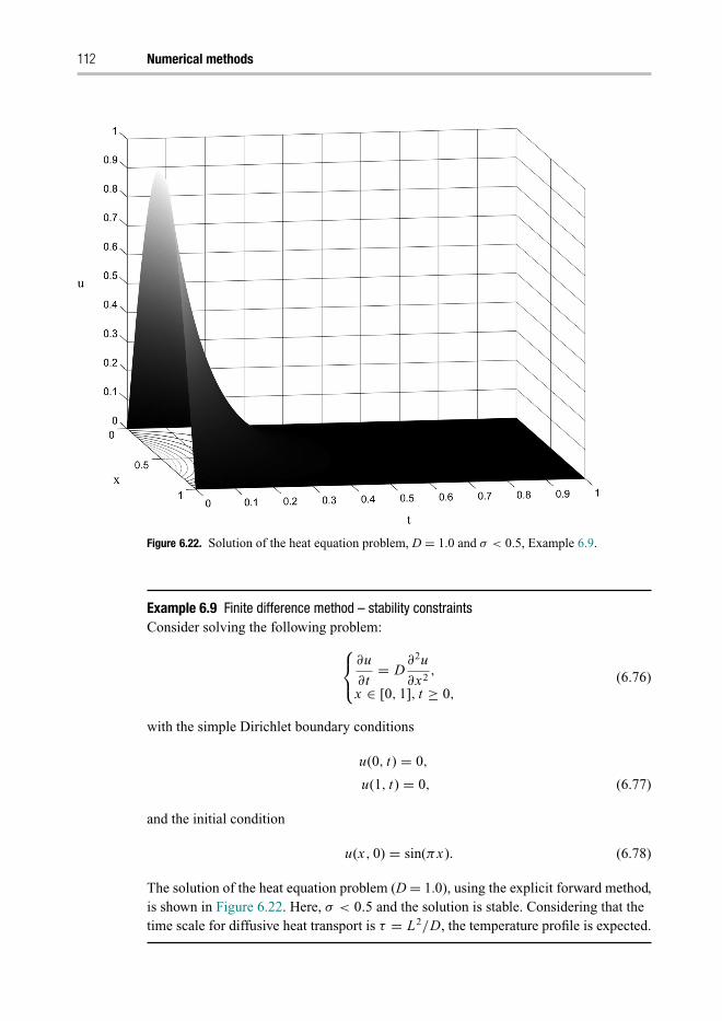
Trim: 247mm × 174mm Top: 12.653mm Gutter: 16.871mmCUUK2531-06 CUUK2531/Rasmuson ISBN: 978 1 107 04969 7 November 13, 2013 17:2
112 Numerical methods
Figure 6.22. Solution of the heat equation problem, D = 1.0 and σ < 0.5, Example 6.9.
Example 6.9 Finite difference method – stability constraintsConsider solving the following problem:⎧⎨
⎩∂u
∂t= D
∂2u
∂x2,
x ∈ [0, 1], t ≥ 0,
(6.76)
with the simple Dirichlet boundary conditions
u(0, t) = 0,
u(1, t) = 0, (6.77)
and the initial condition
u(x, 0) = sin(πx). (6.78)
The solution of the heat equation problem (D = 1.0), using the explicit forward method,is shown in Figure 6.22. Here, σ < 0.5 and the solution is stable. Considering that thetime scale for diffusive heat transport is τ = L2/D, the temperature profile is expected.

Trim: 247mm × 174mm Top: 12.653mm Gutter: 16.871mmCUUK2531-06 CUUK2531/Rasmuson ISBN: 978 1 107 04969 7 November 13, 2013 17:2
6.3 Partial differential equations 113
Figure 6.23. Stability of the forward explicit method for the heat equation. Temperaturedistributions are shown at t = 1; (a) stable for σ = 0.4; (b) unstable for σ = 0.5005.
The instability in the solution of the heat equation problem occurs for σ > 0.5.Figure 6.23(a) shows the temperature profile at t = 1.0 for D = 1.0 and σ = 0.4, andFigure 6.23(b) shows the predicted profile for σ = 0.5005. The instability for σ > 0.5is very clear. The problem with stability can be overcome by using other differencemethods, e.g. implicit methods.
6.3.4 Backward difference method
The implicit backward difference formula,
ut (xi , t j ) = u(xi , t j ) − u(xi , t j−1)
k+ O(k), (6.79)
improves stability. Upon substitution into the heat equation and rearrangement, the PDEis approximated numerically by
1
k(ui, j − ui, j−1) = D
h2(ui+1, j − 2ui, j + ui−1, j ). (6.80)
Stability analysis shows that the backward implicit method is stable for any choice ofstep size k and h. This means that the method is unconditionally stable; as such, thestability does not depend on the σ = k D/h2 value.
As the local error is the same as in the forward difference method, i.e. O(k) + O(h2),the error from the time discretization dominates, assuming step sizes and h � k. Althoughthe method is unconditionally stable, its accuracy is low due to the large local truncationerror. Overall, the backward difference method is O(k), which means that the error at acertain point decreases linearly with k. In other words, if k is cut in half, so is the error.In contrast, if h is cut in half (for a given k), the error would be about the same, and theamount of computation would increase.

Trim: 247mm × 174mm Top: 12.653mm Gutter: 16.871mmCUUK2531-06 CUUK2531/Rasmuson ISBN: 978 1 107 04969 7 November 13, 2013 17:2
114 Numerical methods
6.3.5 Crank–Nicolson method
The Crank–Nicolson method is a combination of implicit and explicit methods, and thebenefit of the method is twofold. First, the method is unconditionaly stable, and secondthe truncation error is smaller, O(k2) +O(h2). Implementing the Crank–Nicolson methodin the heat equation gives
2ui, j − 2ui, j−1 = Dk
h2(ui+1, j − 2ui, j + ui−1, j + ui+1, j−1 − 2ui, j−1 + ui−1, j−1).
(6.81)
This section has provided a short introduction to solving PDEs using the finite differencemethod. But there is much more to explore, and the reader is referred to books onadvanced numerical methods to learn more about how to solve PDEs. In most casesthe reader will use existing numerical algorithms for solving ODEs and PDEs, eithercommercial or open-source. Section 6.4 gives a short description of some of thesesoftware products.
6.4 Simulation software
There are many numerical software products available, both commerical and open-source. It is good practice to use the available algorithms for solving ODEs and PDEsrather than to develop new ones from scratch. In this section we list some of most popularalgorithms in MATLAB, since it is used widely in both academia and industry. Anotherpopular software product is GNU Octave (freeware). Besides these software products,there is a series of useful books on numerical analysis, “Numerical Recipes.”
6.4.1 MATLAB
The two work horses used for solving ODE problems are ode45 for non-stiff equationsand ode15s for stiff equations. These methods have in common that the step size does notneed to be specified, because the solvers include an estimate of the error at each step. Thesolver then adapts the step size to meet the specified error tolerance. The explicit solversare all unstable with stiff systems. The solver will shorten time steps and the solutionwill take a long time, or the step reduces to a point where machine precision causes thealgorithm to fail. The most widely used ODE solvers are classified in accordance to theircharacteristics, as discussed in the preceding sections, and as shown in Table 6.5
The MATLAB ODE solvers are given three arguments: the function evaluating theright-hand side of the differential equation; the time interval to integrate over; and theinitial conditions. There are also other important characteristics, besides the ones listedin the table, that might be of importance when selecting a particular algorithm. Forexample, the ode15s solver can solve differential algebraic equations (DAEs).
Methods for solving BVPs and PDEs are summarized in Table 6.6. The standardMatlab installation has one PDE solver. But there is also a toolbox for solving PDEs

Trim: 247mm × 174mm Top: 12.653mm Gutter: 16.871mmCUUK2531-06 CUUK2531/Rasmuson ISBN: 978 1 107 04969 7 November 13, 2013 17:2
6.4 Simulation software 115
Table 6.5. Characteristics of MATLAB ODE-IVP solvers
SolverExplicit/implicit
Single step/multi-step
Non-stiff/stiff Accuracy Method
ode23 explicit single non-stiff low Runge–Kutta pair of order 2 and 3, of Bogackiand Shampine
ode45 explicit single non-stiff medium Runge–Kutta pair of order 4 and 5, ofDormand–Prince
ode113 explicit multi non-stiff variable lowto high
Adams–Bashforth–Moultonpredictor–corrector pairs of order 1 to 13
ode15s implict multi stiff variable lowto medium
numerical differentiation formulas, orders 1to 5
ode23s implicit single stiff low modified Rosenbrock formula of order 2
Table 6.6. BVP and PDE solvers
Method Category Comment
bvp4c boundary value solves two-point BVPs for ODEspdepe parabolic and elliptic, PDEs PDE solver for parabolic-elliptic PDEspdetool PDEs graphical user interface to solve PDEs
Table 6.7. Minimization and root-finding methods
Method Comment
fzero finds zero of single-variable functionfsolve solves system of equations of several variablesfminunc finds a minimum of a scalar function of several variables, unconstrainedfmincon finds a constrained minimum of a scalar function of several variableslsqnonlin solves non-linear least-square problems, e.g. regression analysis (see Chapter 7)
in which the command pdetool invokes a graphical user interface (GUI). In this GUI,the user can draw geometry, define boundary conditions, specify the PDE, generate themesh, and compute and display the solution. It allows the solution of PDEs in two spacedimensions and time.
6.4.2 Miscellaneous MATLAB algorithms
For the convenience of MATLAB beginners, we list some other useful algorithms in theTables 6.7 and 6.8. Some of these algorithms and commands might assist in completingthe practice problems.
Linear equation systems can be solved with the linsolve algorithm. Various post-processing and visualization commands are available, as shown in Table 6.8.

Trim: 247mm × 174mm Top: 12.653mm Gutter: 16.871mmCUUK2531-06 CUUK2531/Rasmuson ISBN: 978 1 107 04969 7 November 13, 2013 17:2
116 Numerical methods
Table 6.8. Visualization of the solution
Method Comment
plot linear plot, 2Dloglog log-log plot, 2Dcontour3 creates a 3D contour plot of a surfacesurf colored surface plot 3D
Analytical solutions of some ODEs can be obtained with dsolve. As an example, asolution to a particle settling at low particle Reynolds number can be obtained with the“Symbolic toolbox” in MATLAB:
y=dsolve(’Dy=k1-k2*y’,’y(0)=0’,’t’)
which gives
y = (k1 -- k1/exp(k2*t))/k2
6.4.3 An example of MATLAB code
The solution to one of the problems in Example 6.1,⎧⎪⎪⎪⎨⎪⎪⎪⎩
dy
dx= f (x, y) = y + x,
y(0) = 1,
x ∈ [0, 1],
can be obtained by the following commands in the MATLAB prompt.
opts = odeset(’RelTol’, 1e--4);
[x,y] = ode45(@f, [0 1], 1, opts)
plot(x,y)
and by specifying the differential equation in a function file (m-file),
function dy = f(x,y)
dy = y + x;
Note that the Matlab ODE solver is given three arguments: the function evaluating theright-hand side of the differential equation, the time interval to integrate over, and theinitial conditions. The first line of code (opts) sets the relative error tolerance to 1e-4(default is 1e-3). This line is followed by a command which calls the ode45 solver, andspecifies that the differential equation is specified in the m-file. Further, the commandalso specifies that the ODE should be solved in the interval 0–1 and at the initial conditiony0 =1. The third line is just used to plot the solution in a graph.

Trim: 247mm × 174mm Top: 12.653mm Gutter: 16.871mmCUUK2531-06 CUUK2531/Rasmuson ISBN: 978 1 107 04969 7 November 13, 2013 17:2
6.6 Questions 117
It is also possible to solve the problem by defining the function f (x, y) “inline”:
[x,y] = ode45(inline(’y+x’,’x’,’y’), [0 1], 1, opts)
6.4.4 GNU Octave
Octave is a programming language with syntax very similar to that in MATLAB. It isused in academia and industry for numerical analysis. The software is available for freeunder the terms of the GNU General Public License and runs on both Windows andUnix systems.
6.5 Summary
Differential equations play a dominant role in modeling chemical engineering systems.This chapter has explained the principles underlying solutions to differential equations.The purpose was to introduce the concepts of accuracy, stability, and computational effi-ciency. With this knowledge, the reader can understand how different algorithms work,and how to select appropriate numerical algorithms for different kinds of differentialequations. Readers who are particularly interested in this area are encouraged to studymore advanced books on numerical analysis for more details.
6.6 Questions
(1) What is the difference between the local truncation error and the global error, andhow are they related?
(2) How can error tolerance be ensured when a true solution does not exist whensolving differential equations?
(3) Explain what is meant by adaptive step size methods, and why they are used.
(4) What characterizes multi-step methods, and why are they often used?
(5) How do predictor–corrector pairs work, and why are they used?
(6) How is stability related to explicit and implicit methods, and what is a conditionallystable method?
(7) Explain what is meant by stiff differential equations, and what category of ODEsolvers is suitable for stiff systems.
(8) Why are different solution methods needed for IVPs and BVPs, and how can BVPsbe solved?
(9) Explain the principle behind the finite difference method.
(10) What do the collocation and finite element methods have in common, and how dothey differ?

Trim: 247mm × 174mm Top: 12.653mm Gutter: 16.871mmCUUK2531-06 CUUK2531/Rasmuson ISBN: 978 1 107 04969 7 November 13, 2013 17:2
118 Numerical methods
6.7 Practice problems
There are many books on numerical methods available that contain exercises that allowyou to practice writing your own algorithms to solve differential equations. It is equallyimportant to learn how to use the existing software products for numerical analysis,and select appropriate numerical methods for stability and efficiency reasons. With thisin mind, some of the problems in this section require that you work with software fornumerical computing, e.g. MATLAB.
6.1 Find the approximate solution to the IVP dy/dt = t − y, y(0) = 1, for t ∈ [0, 1],using step sizes h = 0.1, 0.01, and 0.001. Determine the error at t =1 and make alog-log plot of the global error as a function of the step size h, using(a) the forward Euler method,(b) the fourth-order Runge–Kutta method.(c) Confirm that the two lines are consistent with the order of the method.The analytical solution is y(t) = t + 2/et − 1.
6.2 Apply the explicit and implicit Euler methods to find an approximate solution to thefollowing IVPs:
(a)dy
dt= 50(1 − y), y(0) = 0.5, t ∈ [0, 1];
(b)dy
dt= 50(y − y2), y(0) = 0.5, t ∈ [0, 1].
Plot the solutions for different step sizes. What step size is required for the explicitmethod to converge to the equilibrium value? Recall that Newton’s method to find aroot of z(x) = 0 and starting guess, x0, is xi+1 = xi − [z(xi )/z′(xi )].
6.3 Write the higher-order differential equation as a system of first-order differentialequations:
(a)d2 y
dx2+ x2 dy
dx− y sin(x) = 0;
(b)d2 y
dx2− y
dy
dx+ x2 − α = 0;
(c)d3 y
dx3− d2 y
dx2
dy
dx+ y2 − ex = 0;
(d)d4 y
dx4− dy
dxy2 + ex = 0.
6.4 Depending on the rate constants, chemical reacting systems might be stiff. Onewell-known stiff system is the Robertson example, which consists of non-linearODEs characterized by a large difference in the rate constants. The three reactionsoccurring in the system are
Ak1−→ B,
B + Bk2−→ B + C,
B + Ck3−→ A + C,

Trim: 247mm × 174mm Top: 12.653mm Gutter: 16.871mmCUUK2531-06 CUUK2531/Rasmuson ISBN: 978 1 107 04969 7 November 13, 2013 17:2
6.7 Practice problems 119
where the rate constants are k1 = 0.04, k2 = 3.107, k3 = 1 · 104, and the initial con-centrations of the three species are CA0 = 1, CB0 = 0, and CC0 = 0.(a) Assume the reactions are carried out in a batch reactor operated at isothermal
conditions, and derive the system of ODEs.(b) Use a solver suitable for stiff problems and plot the solution for t ∈ [0, 100].(c) Evaluate the performance of non-stiff and stiff solvers, e.g. MATLAB ode45 and
ode15s, by analyzing the number of steps required by the two different solvers.(d) Determine how the order of the method for stiff solvers is related to the error
tolerance specified.
6.5 An ideal batch reactor is used to hydrogenate compound A. The hydrogen is fedthrough a gas sparger and dissolves in the liquid phase, where it reacts with com-pound A,
A + H2r−→ B,
where the reaction rate is r = kCACH2 and k = 10−3 m3 s−1 mol−1.The hydrogen mass transfer rate is dominated by the liquid film resistance. This
allows the mass transfer rate to be modeled as Na = kLa(CiH2
− CH2 ), where kLa =10 s−1. The initial concentration of compound A is C0
A = 10[mol m−3], and, ashydrogen is replenished to maintain the reactor pressure, Ci
H2= 0.1[mol m−3].
(a) Derive the material balances that describe how the concentrations CA and CH2
vary in time. Assume perfect mixing and isothermal conditions in the reactor.(b) Estimate the time constants and select a suitable ODE solver.(c) Make a plot that shows how the concentrations change in time.
6.6 Diffusion and reaction inside a spherical catalyst particle are described by thefollowing BVP:
d2C
dr2+ 2
r
dC
dr− 4C = 0,
C(1) = 1,
dC
dr
∣∣∣∣r=0
= 0,
r ∈ [0, 1].
(a) Use the collocation method, with a collocation point at r = 0.5, to find anapproximate solution. The result can be compared with the concentration profileshown in Figure 6.13.
(b) Use the MATLAB built-in BVP solver to find the solution to the problem.
6.7 Heat transport by conduction is described by the parabolic PDE
∂T
∂t= D
∂2T
∂x2,
x ∈ [0, 1], t ∈ [0, 1],
the boundary conditions T (0, t) = 0 and T (1, t) = 0, the initial condition T (x, 0) =sin2(4πx), and the heat diffusivity D = λ/ρcp = 1. Find the solution by
Trim: 247mm × 174mm Top: 12.653mm Gutter: 16.871mmCUUK2531-06 CUUK2531/Rasmuson ISBN: 978 1 107 04969 7 November 13, 2013 17:2
120 Numerical methods
(a) using the finite difference, forward time central space, method;(b) using the finite difference, Crank–Nicolson, method;(c) using the MATLAB built-in PDE solver “pdepe”.
6.8 A metal rod initially at ambient air temperature, 25 °C, is connected on one sideto a wall at constant temperature 100 °C, and the other side is surrounded by air.Heat conduction through the rod and losses by convection to the surroundings arebalanced by accumulation of thermal energy in the rod. The energy balance is givenby
∂T
∂t= λ
ρcp
∂2T
∂x2− k1(T − Ts),
where Ts = 25 °C is the surrounding air temperature (constant) and k1 =5.25 · 10−7 s−1 (depends amongst other things on the heat conduction in air and theradius of the rod). The rod is 1 m long and made of silver; the corresponding materialdata for silver is λ = 424 W m−1 K−1, ρ = 10 500 kg m−3, and cp = 236 J kg−1 K−1.(a) Propose a suitable boundary condition for the tip of the rod, which is in contact
with air.(b) Estimate the time constant of the system.(c) Determine how the temperature profile evolves in time.

Trim: 247mm × 174mm Top: 12.653mm Gutter: 16.871mmCUUK2531-07 CUUK2531/Rasmuson ISBN: 978 1 107 04969 7 November 13, 2013 17:33
7 Statistical analysis ofmathematical models
7.1 Introduction
In chemical engineering, mathematical modeling is crucial in order to design equipment,choose proper operating conditions, regulate processes, etc. It is almost always necessaryto use experimental data for model development. Figure 7.1(a) shows a data set andlinear fit for these data. From this result, is easy to see that this line describes these data.However, from the data set shown in Figure 7.1(b), this is not so clear. The solid linerepresents the linear fit for these data, which is derived from regression analysis. Bysimply observing the data, it can be seen that either of the dashed lines could be possiblefits. These results clearly show that it is not possible to determine parameters for modelsonly by which line looks a good fit, but that a detailed statistical analysis is needed.
In this chapter, we start by describing linear regression, which is a method for deter-mining parameters in a model. The accuracy of the parameters can be estimated by confi-dence intervals and regions, which will be discussed in Section 7.5. Correlation betweenparameters is often a major problem for large mathematical models, and the determi-nation of so-called correlation matrices will be described. In more complex chemicalengineering models, non-linear regression is required, and this is also described in thischapter.
7.2 Linear regression
Regression analysis is a statistical method for determining parameters in models. Thesimplest form is a first-order straight-line model, which can be described by
y = β0 + β1x + ε, (7.1)
where
y is the dependent variable that can also be called the response variable;x is the predictor of y, also known as the regressor or independent variable;βi are parameters;ε is the stochastic part, and describes the random error.
In this chapter, the vectors and matrices will be written in bold italic style. Thestraight-line model can be divided into two parts: the deterministic part, E( y), and

Trim: 247mm × 174mm Top: 12.653mm Gutter: 16.871mmCUUK2531-07 CUUK2531/Rasmuson ISBN: 978 1 107 04969 7 November 13, 2013 17:33
122 Statistical analysis of mathematical models
Figure 7.1. Data sets and corresponding linear fits.
Figure 7.2. Simple linear regression model.
the stochastic part, ε. The term E( y) is also called the expectation function, and it isdescribed by
E( y) = β0 + β1x. (7.2)
Figure 7.2 shows a straight-line fit. The slope of the line represents β1 and the y-intercept β0 in Equation (7.1). The errors ε1 for x = x1 and ε2 for x = x2 are also shownin the figure.
A more general equation for the linear regression is the so-called multiple linearregression that is described by
y = β0 + β1x1 + β2x2 + · · · + βk xk + ε, (7.3)
where x1 and x2 could be different variables for, e.g., pressure and temperature, butmay also be powers of x, x2, x3, etc. This equation is denoted linear by virtue of itslinear parameters. This can also be seen by the fact that d y/dβ is only a function ofthe independent variables, x. To illustrate linear models further, some examples aregiven. The model in Equation (7.4) is linear in its parameters and is called a polynomialmodel:
y = β0 + β1x + β2x2 + β4x4 + ε. (7.4)

Trim: 247mm × 174mm Top: 12.653mm Gutter: 16.871mmCUUK2531-07 CUUK2531/Rasmuson ISBN: 978 1 107 04969 7 November 13, 2013 17:33
7.2 Linear regression 123
Another set of models, which are also linear with respect to the parameters, are theso-called sinusoidal models:
y = β0 + β1 sin(θ ) + β2 cos(θ) + ε. (7.5)
An example of a non-linear model is the Arrhenius equation, which is very importantfor describing the temperature dependence of the rate constants. It is given by
k = Ae−E A/RT , (7.6)
where k is the rate constant, A is the pre-exponential factor, EA is the activation barrier,R is the general gas constant, and T is the temperature. The rate constant is includedin the material and heat balances for a system, with the result that the concentrationsand temperature depend on the parameters in the rate constants. The parameters of thisequation that should be determined are A and EA. Re-writing Equation (7.6) using thenotation in Equation (7.3) would result in
k = β0e−β1/Rx . (7.7)
This yields
dk
dβ1= −β0
Rxe−β1/Rx,
and as this derivative contains β1 it means that it is not linear in the parameter β1;therefore this is a non-linear model.
7.2.1 Least square method
The least square method is a statistical approach used to estimate the parameters pre-viously described. First, we will consider the simplest case, which is the first-orderstraight-line model. This model is described by
y = β0 + β1x + ε. (7.8)
The sum of square errors is denoted by SSE, or s, and is described by
SSE =∑n
i=1ε2
i , (7.9)
where ɛi is the random error at the experimental point i (see Figure 7.2). To illustratethis further, if there were experimental points x1, x2, x3, x4, . . . , xn, the correspondingerrors would be described by ε1, ε2, ε3, ε4, . . . , εn . These errors for experimental pointi would be expressed by
εi = yi − (β0 + β1xi ). (7.10)
This means that the error in each point is the difference between the experimentallymeasured value and the value calculated by the model. In the least square method, theSSE described in Equation (7.9) is minimized. The resulting line, when SSE is at a

Trim: 247mm × 174mm Top: 12.653mm Gutter: 16.871mmCUUK2531-07 CUUK2531/Rasmuson ISBN: 978 1 107 04969 7 November 13, 2013 17:33
124 Statistical analysis of mathematical models
minimum, is known as the least square, or regression, line. The true model is describedby
y = β0 + β1x + ε, (7.11)
and the estimated regression line can be described by
y = b0 + b1x, (7.12)
where b0 and b1 are estimates of the true β0 and β1, respectively, and y is the y predictedby the model. When minimizing SSE, the normal equations are set up. This will beperformed for the simplest case, the first-order straight-line model. The least squareerror is minimized when the derivative with respect to the two parameters equals zero:
∂SSE
∂β0= 0, (7.13)
∂SSE
∂β1= 0, (7.14)
where the least square error is given by
SSE =n∑
i=1
ε2i =
n∑i=1
(yi − (β0 + β1xi ))2. (7.15)
When using the expression for SSE in Equation (7.15) and differentiating it withrespect to each parameter, the following expressions are obtained:
∂SSE
∂b0=
n∑i=1
2(yi − (b0 + b1xi ))(−1) = 0; (7.16)
∂SSE
∂b1=
n∑i=1
2(yi − (b0 + b1xi ))(−xi )
= 2n∑
i=1
(yi xi − (b0xi + b1x2i )) = 0 (7.17)
Simplifications of Equations (7.16) and (7.17) result in
n∑i=1
(yi ) − nb0 − b1
n∑i=1
(xi ) = 0, (7.18)
n∑i=1
(yi xi ) − b0
n∑i=1
(xi ) − b1
n∑i=1
(x2i ) = 0. (7.19)
Equations (7.18) and (7.19) are often denoted as normal equations. The parametersb0 and b1 can be easily retrieved from these equations. Often, the averages of y and x,respectively, are used. They are denoted by x and y, and are given by
x = 1
n
n∑i=1
(xi ) (7.20)

Trim: 247mm × 174mm Top: 12.653mm Gutter: 16.871mmCUUK2531-07 CUUK2531/Rasmuson ISBN: 978 1 107 04969 7 November 13, 2013 17:33
7.3 Linear regression in its generalized form 125
and
y = 1
n
n∑i=1
(yi ). (7.21)
This results in
b0 = y − b1 x (7.22)
and
b1 =∑n
i=1 (xi − x)(yi − y)∑ni=1 (xi − x)2 . (7.23)
7.3 Linear regression in its generalized form
As discussed in Section 7.2, a multiple linear regression can be described by
y = β0 + β1x1 + β2x2 + · · · + βk xk + ε. (7.24)
This equation can be written in a more generalised matrix form as follows:
y = Xβ + ε, (7.25)
where the vectors and matrices y, X, β and ε are defined as
y =
⎡⎢⎢⎢⎢⎢⎣
y1
y2
y3...yn
⎤⎥⎥⎥⎥⎥⎦ , X =
⎡⎢⎢⎢⎢⎢⎣
1 x11 x12 x13 · · · x1k
1 x21 x22 x23 · · · x2k
1 x31 x32 x33 · · · x3k...
......
......
1 xn1 xn2 xn3 · · · xnk
⎤⎥⎥⎥⎥⎥⎦ , β =
⎡⎢⎢⎢⎢⎢⎣
β0
β1
β2...βk
⎤⎥⎥⎥⎥⎥⎦ , ε =
⎡⎢⎢⎢⎢⎢⎣
ε1
ε2
ε3...εn
⎤⎥⎥⎥⎥⎥⎦ .
(7.26)
The dimensions of these matrices are n × 1 for y, n × p for X, p × 1 for β, and n × 1for ε, where p is the number of parameters and is equal to k + 1 and n is the numberof experimental points. As before, E is the expectation operator, and the expectationfunction is denoted by
E( y) = Xβ. (7.27)
The vector of expected values for the error is 0, i.e.
E(ε) = 0. (7.28)
The variance of the error is denoted by σ 2, and can be written using the variance, V:
V (ε) = σ 2. (7.29)
In many experiments, the expected error is not constant for all observation points. Wecan still make a least squares minimization, but we cannot make any statistical analysisunless we stabilize the variance (see Section 7.4). For a detailed statistical analysis, eachobservation should be weighted with its variance.

Trim: 247mm × 174mm Top: 12.653mm Gutter: 16.871mmCUUK2531-07 CUUK2531/Rasmuson ISBN: 978 1 107 04969 7 November 13, 2013 17:33
126 Statistical analysis of mathematical models
Figure 7.3. Two data sets with (a) small and (b) large variance, respectively.
To illustrate further the importance of the variance, two different data sets are shown inFigure 7.3. The data in Figure 7.3(a) have a small variance, whilst the data in Figure 7.3(b)have a large variance. The variance will be determined using so-called analysis ofvariance (ANOVA) tables, which will be described in detail in Section 7.8.2.
7.3.1 Least square method
The least square method is used for determining the parameters in the regression model,as described in Section 7.2.1. The sum of square error is given by
SSE =n∑
i=1
ε2i . (7.30)
When using models in a more generalized matrix form, the residual sum of squaresis defined by
SSE = ( y − Xβ)′( y − Xβ). (7.31)
In the same way as for the simple case of the straight-line model, the sum of squaresis minimized when the derivate of SSE with respect to the parameters is set at zero. Thisresults in
∂SSE
∂β
∣∣∣∣b
= 0, (7.32)
where b (p × 1) is a vector with the estimated parameters. In Equation (7.31), SSE canbe further developed into
SSE = y′ y − y′ Xβ − β ′x′ y + β ′ X ′ Xβ
= y′ y − 2β ′ X ′ y + β ′ X ′ Xβ. (7.33)
The derivative of SSE with respect to β gives
∂SSE
∂β
∣∣∣∣b
= −2X ′ y + 2X ′ Xb = 0. (7.34)
This is the normal equation in matrix form. This equation can be rearranged to yield
X ′ y = X ′ Xb, (7.35)

Trim: 247mm × 174mm Top: 12.653mm Gutter: 16.871mmCUUK2531-07 CUUK2531/Rasmuson ISBN: 978 1 107 04969 7 November 13, 2013 17:33
7.4 Weighted least squares 127
which can be used to retrieve an equation for determining the parameter vector b:
b = (X ′ X)−1 X ′ y. (7.36)
The basis for this equation is that the expected value for the error is 0, i.e.
E(ε) = 0, (7.37)
and the variance of ε is σ 2, which can be written using the variance, V :
V (ε) = σ 2. (7.38)
7.4 Weighted least squares
Weighted least squares are important and have several different applications. Examplesof cases where weighted least squares are important include:
(1) stabilization of the variance;(2) placing greater/less weight on certain experimental parts.
These two topics will be discussed in Sections 7.4.1 and 7.4.2.
7.4.1 Stabilization of the variance
Stabilizing the variance is the fundamental reason behind weighted residuals, where eachexperiment is weighted against its variance. The reason for doing this is that in manyexperiments the expected error is not equal in different observations. For these cases, inorder to make a detailed statistical analysis we should weight each measurement with itsvariance. If adding weight factors, wi, where the variance for each experiment is dividedby the variance, this results in
wi =(σi
σ
)2. (7.39)
In many types of analytical equipment, the error is a fixed percentage of the maximuminstrument reading, which results in a variance proportional to yi, i.e. σi ∝ yi . This givesan uneven variance distribution that calls for using a weight factor, for example 1/yz
i ,
or a logarithm:
zi = ln yi . (7.40)
If zi is differentiated, we obtain
dzi = 1
yidyi , (7.41)
which means that dzi corresponds to a small error in yi divided by yi (dyi/yi ) that yieldsthe weight factor 1/y2
i . Weight factors are discussed further in the context of residualplots in Section 7.8.1.

Trim: 247mm × 174mm Top: 12.653mm Gutter: 16.871mmCUUK2531-07 CUUK2531/Rasmuson ISBN: 978 1 107 04969 7 November 13, 2013 17:33
128 Statistical analysis of mathematical models
Figure 7.4. Two experimental outliers in a data set.
7.4.2 Placing greater/less weight on certain experimental parts
Another reason for using weight factors is to vary the weight according to differentparts of an experiment. Figure 7.4 shows an example where a large set of data showsa clear linear trend. However, two experimental points deviate significantly (markedby arrows in Figure 7.4). These types of data points that exhibit clear deviations fromthe others are denoted “outliers” and are occasionally present in experimental series. Ifexperimental outliers are found, the best procedure would be to repeat the experimentfor these two points a few additional times to verify the observations. However, it is notalways possible to redo the experiments. One possibility, for these cases, could be toplace a lower weight on the error for these measuring points. It is also possible to removethese outliers in the regression analysis. However, if outliers were removed during theregression, it would be critical to add them to the figures, clearly indicating that theweight factor for these outliers would be zero (or another appropriate value).
The outliers in the example of Figure 7.4 do not substantially influence the regressionmodel because one outlier is below the line and another is above the line. The dashed linein Figure 7.4 (which is almost on top of the solid line) shows the resulting regressionline if both points were removed in the least square analysis. The fact that the twolines are roughly in the same position means that these outliers have only minor effecton the regression. Another case is shown in Figure 7.5, where there is a single outlier. Inthe same way as in Figure 7.4, the dashed line shows the regression line when removingthe outlier (using a weight factor of zero on that point). In this case, this outlier has aclear impact on the least square estimation. It should be emphasized that outliers cannotbe removed without a clear motivation, and that, if weight factors were used, they wouldhave to be thoroughly described.
Recall the equation for the linear models,
y = β0 + β1x1 + β2x2 + · · · + βk xk + ε, (7.42)
where
SSE =n∑
i=1
e2i =
∑n
i−1(yi − yl)
2. (7.43)

Trim: 247mm × 174mm Top: 12.653mm Gutter: 16.871mmCUUK2531-07 CUUK2531/Rasmuson ISBN: 978 1 107 04969 7 November 13, 2013 17:33
7.4 Weighted least squares 129
Figure 7.5. Effect of one experimental outlier on the regression model.
Figure 7.6. Model and experimental data for ammonia storage and desorption over a catalyst.From Olsson, L., Sjovall, H., and Blint, R. J., Appl. Catal. B 81, 203–207, 2008. Reproducedwith permission from Elsevier.
For the case using weight factors, the weighted sum of square errors, WSSE, can beexpressed as follows:
WSSE =n∑
i=1
wi e2i =
n∑i=1
wi (yi − yi )2. (7.44)
In this section, we have described cases when experimental data points are not fullyreliable, which might be the case with outliers. Another key area for weighted residuals iswhen certain parts of the experiment are very important and we would like to emphasizethose parts of the regression model. An example from our research on automotivecatalysis is depicted in Figure 7.6. In this experiment, the catalyst is exposed to ammoniafor 80 min and the experimental (solid line) and simulated (dashed line) outlet ammoniaconcentration are shown in the figure. Initially, ammonia adsorbs on the catalyst, whichis why the outlet ammonia concentration is zero. When the catalyst is saturated, ammonia

Trim: 247mm × 174mm Top: 12.653mm Gutter: 16.871mmCUUK2531-07 CUUK2531/Rasmuson ISBN: 978 1 107 04969 7 November 13, 2013 17:33
130 Statistical analysis of mathematical models
breaks through. Thereafter, the ammonia is turned off and the temperature is increased,which results in an ammonia desorption peak. The binding strength can be receivedduring the temperature ramp, so the desorption part is far more critical than the adsorptionpart when tuning a model to the data. However, the concentration in the desorption is quitelow, with the result that, in a standard fitting procedure, the adsorption part influencesthe parameters in the model to a greater extent. Since the desorption part is far moreimportant to the kinetic model, this is not the desired situation. In this case, weightedresiduals can be used, where the error during the desorption part has a larger weightfactor compared to the adsorption. In the example shown in Figure 7.6, the model isnon-linear but the interpretation of weighted residuals remains the same.
Different weight factors can also be applied to the residual sum of squares when theresponse variables have varying orders of magnitude. For example, for models describingemission cleaning with the help of catalysis, it is common to use both molar fractionsand temperatures as response variables. In many cases, the molar fraction is in the range100 × 10−6–500 × 10−6, and the temperature is 400–700 K. If no weight factor wereapplied in this case, the errors in the prediction of the temperature would totally dominateand the molar fraction would have only a minor influence. However, as the errors inthe molar fractions are crucial, this is not a good solution. Therefore, a weight factorcan be applied to the molar fractions, with the result that the errors are similar in sizeto those for the temperatures (the opposite would also be possible using a smaller factoron the temperature instead).
7.5 Confidence intervals and regions
7.5.1 Confidence intervals
The basis for confidence intervals is that the error is normally distributed with thevariance σ 2, i.e. ε ∼ N (0, Iσ 2). This also results in b being normally distributed and
E(b) = β. (7.45)
The variance, s2, can be estimated by dividing the sum of square errors, SSE, by thedegrees of freedom, v
v = n − p, (7.46)
s2 = SSE
v= SSE
n − p(7.47)
where n is the number of experimental data points and p is the number of parametersin the model. Equation (7.46) applies to the case for which there is only one sourceof errors. The estimation of the degrees of freedom, v, will be discussed in detail inSection 7.5.1.1. The standard error of the parameter p is calculated according to:
se(bp) = s√
{(X ′ X)−1}pp, (7.48)
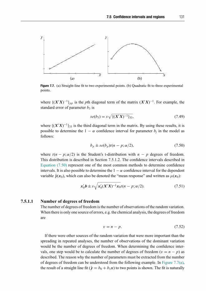
Trim: 247mm × 174mm Top: 12.653mm Gutter: 16.871mmCUUK2531-07 CUUK2531/Rasmuson ISBN: 978 1 107 04969 7 November 13, 2013 17:33
7.5 Confidence intervals and regions 131
Figure 7.7. (a) Straight-line fit to two experimental points. (b) Quadratic fit to three experimentalpoints.
where {(X ′ X)−1}pp is the pth diagonal term of the matrix (X ′ X)−1. For example, thestandard error of parameter b3 is
se(b3) = s√
{(X ′ X)−1}33, (7.49)
where {(X ′ X)−1}33 is the third diagonal term in the matrix. By using these results, it ispossible to determine the 1 − α confidence interval for parameter bj in the model asfollows:
bp ± se(bp)t(n − p; α/2), (7.50)
where t(n − p; α/2) is the Student’s t-distribution with n − p degrees of freedom.This distribution is described in Section 7.5.1.2. The confidence intervals described inEquation (7.50) represent one of the most common methods to determine confidenceintervals. It is also possible to determine the 1 − α confidence interval for the dependentvariable y(x0), which can also be denoted the “mean response” and written as μ(x0):
x′0b ± s
√x′
0(X ′ X)−1x0t(n − p; α/2). (7.51)
7.5.1.1 Number of degrees of freedomThe number of degrees of freedom is the number of observations of the random variation.When there is only one source of errors, e.g. the chemical analysis, the degrees of freedomare
v = n − p. (7.52)
If there were other sources of the random variation that were more important than thespreading in repeated analyses, the number of observations of the dominant variationwould be the number of degrees of freedom. When determining the confidence inter-vals, one step would be to calculate the number of degrees of freedom (v = n − p) asdescribed. The reason why the number of parameters must be extracted from the numberof degrees of freedom can be understood from the following example. In Figure 7.7(a),the result of a straight line fit ( y = b0 + b1x) to two points is shown. The fit is naturally

Trim: 247mm × 174mm Top: 12.653mm Gutter: 16.871mmCUUK2531-07 CUUK2531/Rasmuson ISBN: 978 1 107 04969 7 November 13, 2013 17:33
132 Statistical analysis of mathematical models
Figure 7.8. NO, NO2, NH3, and N2O concentration after an ammonia selective catalytic reduction(SCR) experiment over a copper–zeolite catalyst. The inlet gas composition is 400 ppm NOx
(NO or NO2), 400 ppm NH3, and 8% O2. From Sjovall, H., Olsson, L., Fridell, E., and Blint,R. J., Appl. Catal. B 64, 180–188, 2006. Reproduced with permission from Elsevier.
perfect because there is only one way in which a line can be drawn between two points.The number of degrees of freedom for this case is therefore
v = n − p = 2 − 2 = 0. (7.53)
Thus there are no observations of the random error and consequently no degrees offreedom. Similar results can be obtained if a quadratic model
(y = b0 + b1x + b2x2
)were used to fit three experimental points. For this case, the number of degrees offreedom would be zero as well (v = n − p = 3 − 3 = 0).
The number of parameters in the model, p, is often easily calculated. The degrees offreedom is calculated using n − p (see Equation (7.53)), and this example illustrates thedifficulties that can arise when we determine n and thereby v. However, the number ofdata points, n, is not always trivial to determine.
An example will be used to illustrate the number of degrees of freedom. In Figure 7.8,the experimental results from one ammonia selective catalytic reduction (SCR) experi-ment are shown. In this experiment, a copper–zeolite catalyst was exposed to ammoniaNOx (NO + NO2) and oxygen, while varying the NO2 to NOx ratio. The outlet concen-trations of NO, NO2, NH3, and N2O were measured and are depicted in Figure 7.8. Ifthese data points were used in a model, what would the number of degrees of freedombe?
The experiment was 160 min long and measurement points were taken approximatelyevery 6 s, resulting in 1600 data points for each of the four gases, i.e. a total of 6400 datapoints. However, this does not mean that n-6400. This is because we have seven differentconditions (varying NO2 to NOx ratio) and each condition takes a long time to reachsteady-state conditions. Thus, the concentrations are constant in the final part of theexperiment for each condition and therefore n is significantly lower than 6400. However,

Trim: 247mm × 174mm Top: 12.653mm Gutter: 16.871mmCUUK2531-07 CUUK2531/Rasmuson ISBN: 978 1 107 04969 7 November 13, 2013 17:33
7.5 Confidence intervals and regions 133
Figure 7.9. Student’s t-distribution for 10 degrees of freedom, showing 95% confidence limit.
since transient effects occur when the gas composition changes due to the accumulationof species on the surfaces, n is much larger than 7 × 4 = 28 (seven conditions and fourgases). In order to determine n, only the points at which the condition is changed orwhen transient effects occur should be considered.
7.5.1.2 Student’s t-distributionAs mentioned earlier, the t-distribution is used to determine confidence intervals. Thet-distribution has two parameters: the number of degrees of freedom, v, and the signif-icance level of the test divided by two (α/2). We have already discussed v thoroughly.Figure 7.9 shows the t-distribution for a case with v = 10 degrees of freedom andα = 0.05. The two tails represent an area of 0.025 each, which is α/2 for each area. Thisresults in a central area of 1 − 2 × 0.025 = 0.95. Thus, the confidence interval whenusing this t-value is at the 95% level. The values for the t-distribution can be found inAppendix C.
The t-distribution for 2, 10, and 1000 degrees of freedom is shown in Figure 7.10. Thex-value for the 95% confidence limit for the three cases is marked. When increasing thedegrees of freedom, and the number of observations of the random variation is increasing,the t-value becomes lower. This results in lower confidence intervals. Note that when thedegrees of freedom → ∞, the t-distribution will equal the normal distribution.
7.5.2 Student’s t-tests of individual parameters
It is possible also to conduct t-tests on individual parameters. For this purpose, tobs iscalculated according to
tobs = bp
se(bp), (7.54)
and this value is compared with the t-value from the t-distribution with n − p degreesof freedom, t(n − p; α/2). If tobs > t(n − p; α/2), the parameter is significant.

Trim: 247mm × 174mm Top: 12.653mm Gutter: 16.871mmCUUK2531-07 CUUK2531/Rasmuson ISBN: 978 1 107 04969 7 November 13, 2013 17:33
134 Statistical analysis of mathematical models
Figure 7.10. Student’s t-distribution for 2, 10, or 1000 degrees of freedom, showing 95%confidence limit.
Figure 7.11. Individual confidence intervals and joint confidence region for a two-parametermodel (y = b0 + b1x).
7.5.3 Confidence regions and bands
Confidence intervals were described in Section 7.5.1. These intervals are individualfor each parameter. The individual confidence intervals for a two-parameter model(y = b0 + b1x) are shown in Figure 7.11, where the dashed lines show the confidenceinterval for each parameter. It is easy to assume that the area inside the dashed rectangleis the confidence region for the combination of these parameters; however, this is notthe case. The joint confidence region for the two parameters is also depicted in the figure.The confidence region accounts for the variation of both parameters simultaneously,

Trim: 247mm × 174mm Top: 12.653mm Gutter: 16.871mmCUUK2531-07 CUUK2531/Rasmuson ISBN: 978 1 107 04969 7 November 13, 2013 17:33
7.5 Confidence intervals and regions 135
Figure 7.12. F-distribution for 10 and 10 degrees of freedom, showing 95% confidence limit.
which is indicated by the solid line in Figure 7.11. The joint confidence region isellipsoidal, whereas the individual levels form a rectangle, differences that are importantto notice.
To calculate the 1 − α confidence region, the following relationship can be used forthe linear case:
(β − b)′ X ′ X(β − b) ≤ ps2 F(p, n − p; α). (7.55)
This yields an elliptical contour. In more general terms, the 1 − α confidence regionis determined by
SSE(β) ≤ SSE(b)
[1 + p
n − pF(p, n − p; α)
], (7.56)
where F(p, n − p; α) is the F-distribution (see Appendix C) for the degrees of freedom,p, and n − p, respectively, at level α. For linear models, the results for the confidenceregions will be the same when using Equation (7.55) or Equation (7.56). Note that forthe F-distribution the level to be used is α, whilst for the t-distribution it is α/2. Thereason for this difference is that the t-distribution is centered around zero and has twotails, whereas the F-distribution is non-symmetrical (and positive), and only has one tail(Figure 7.12).
As described in Section 7.5.1, the 1 − α confidence interval for the dependent variabley(x0) is determined according to
x′0b ± s
√x′
0(X ′ X)−1x0 t(n − p; α/2). (7.57)
If this calculation is performed for several different points (x), a “point-wise confidenceband” is retrieved. It is also possible to determine the 1 − α confidence interval for thevalue predicted, which is obtained when considering all intervals simultaneously, i.e.
x′b ± s√
x′(X ′ X)−1x√
pF(p; n − p; α). (7.58)

Trim: 247mm × 174mm Top: 12.653mm Gutter: 16.871mmCUUK2531-07 CUUK2531/Rasmuson ISBN: 978 1 107 04969 7 November 13, 2013 17:33
136 Statistical analysis of mathematical models
Figure 7.13. Schematic description of the confidence band.
This is denoted the “simultaneous 1 − α confidence band” for the response functionat any x. Note that the confidence band (Figure 7.13) depends on the independentvariable x.
7.6 Correlation between parameters
After a model has been constructed, it is important to determine the correlation betweenthe parameters. If there is high correlation and one parameter is changed, anotherparameter must also change. Multiple choices of parameters can result in a similar sumof square error. In order to determine the correlation between parameters, the varianceand co-variance must be calculated. Therefore, we start with a description of the variancecalculation, followed by the determination of the co-variance, and finally the correlationmatrix.
7.6.1 Variance and co-variance
The variance matrix for the parameters consists of the variance for each parameter in thediagonal and co-variances in the other positions. Equation (7.59) contains an example ofa model with four parameters (b0, b1, b2 and b3) shown to illustrate this relationship:
V (b) = V
⎛⎜⎜⎝
b0
b1
b2
b3
⎞⎟⎟⎠
=
⎡⎢⎢⎣
V (b0) cov(b0, b1) cov(b0, b2) cov(b0, b3)cov(b1, b0) V (b1) cov(b1, b2) cov(b1, b3)cov(b2, b0) cov(b2, b1) V (b2) cov(b2, b3)cov(b3, b0) cov(b3, b1) cov(b3, b2) V (b3)
⎤⎥⎥⎦ . (7.59)
The variance matrix can be determined by the following correlation:
V (b) = (X ′ X)−1σ 2. (7.60)
For the cases when σ 2 is unknown, the estimated variance, s2, can be used instead.

Trim: 247mm × 174mm Top: 12.653mm Gutter: 16.871mmCUUK2531-07 CUUK2531/Rasmuson ISBN: 978 1 107 04969 7 November 13, 2013 17:33
7.6 Correlation between parameters 137
7.6.2 Correlation matrix
The correlation matrix, C, can be retrieved from the variance matrix according to thefollowing equation:
Ci j = cov(bi , b j )√V (bi )V (b j )
. (7.61)
Combining Equations (7.60) and (7.61) results in the following expression:
Ci j = {(X ′ X)−1}i j√{(X ′ X)−1}i i {(X ′ X)−1} j j
, (7.62)
which can be used for determining the correlation.Each component in Ci j is within the range −1–1. If the correlation equals 0, there
would be no correlation between the parameters, and if the correlation is close to 1 or–1, the parameters are highly correlated. This can be a consequence of:
(1) Poor experimental design.(2) Over-parameterizing, i.e. there are too many parameters and not all of them can be
resolved. Over-parameterization can be estimated using the rank of the X ′ X-matrix(or the J ′ J-matrix, for the non-linear case; the Jacobian, J, will be described inSection 7.7.3).
(3) For non-linear models, there can be built-in correlations. An example is when theArrhenius equation is used for determining the rate constant;
k = Ae−E A/RT , (7.63)
where k is the rate constant, A is the pre-exponential factor, EA is the activationbarrier, R is the general gas constant, and T is the temperature. The parameters thatare used in the modeling are A and EA, which are always correlated, at least to someextent.
(4) High correlation can also be obtained if the independent variables are not centeredin a polynom. For example, in the model
y = b0 + b1x + b2x2 + b3x3 + b4x4, (7.64)
the parameters b0, b1, b2, b3, and b4 are correlated because x is always correlatedwith x2, x3, and x4 if x ˃ 0, for all x. This model can be centered by
xcentered = x − x, (7.65)
where x is the mean of x. However, even for this model, there is a correlation betweenb0 and b2, because (x − x)2 > 0 for all x. This is also the case for x4. Likewise, inthe non-linear case, it is recommended that the data are centered in order to decreasethe correlation between the parameters. One example is the Arrhenius equation,Equation (7.63), in which the temperature can be centered by using a referencetemperature, Tref, which can be chosen to be the mean temperature. This gives
k = A exp
[E A
R
(1
T− 1
Tre f
)](7.66)

Trim: 247mm × 174mm Top: 12.653mm Gutter: 16.871mmCUUK2531-07 CUUK2531/Rasmuson ISBN: 978 1 107 04969 7 November 13, 2013 17:33
138 Statistical analysis of mathematical models
and results in a lower correlation between the parameters when doing the regressionanalysis. This transformation will not affect the activation energy, but the pre-exponential factor will be the rate constant at T = Tref.
7.7 Non-linear regression
In chemical engineering, many models are non-linear, which means that they are non-linear with respect to the parameters. This will be illustrated by a few examples below.The simple straight-line model,
y = b0 + b1x, (7.67)
is of course linear. However, the following models (because they are linear in theparameters) are also linear. Note that the regressor, x, can have different exponents, sineform, etc., while the model remains linear. We have
y = β0 + β1x + β2x2 + β3x4 + βx6; (7.68)
y = β0 + β1 sin(x) + β2 cos(x). (7.69)
However, due to the form of the parameters, the following models are non-linear:
y = θ0 + eθ1 x ; (7.70)
y = θ0 + θ1 sin(θ2x) + θ3 cos(θ4x). (7.71)
In order to separate clearly the linear and non-linear models, we denote the parametersfor the linear models as β i, and that for the non-linear models as θ i. In this chapter, wediscuss the statistical evaluation of non-linear models, which is often very complex;therefore, iterative numerical solutions will be used.
7.7.1 Intrinsically linear models
The models described in Equations (7.70) and (7.71) are non-linear. It is possible totransform some non-linear models into linear models; these types of models are referredto as “intrinsically linear.” It is important to note that the disturbance term is alsotransformed when transforming a model. We present two examples of models that canbe transformed and are thereby intrinsically linear. For catalytic reactions, the reactionrate may contain an inhibition term in the denominator. The reaction rate at constanttemperature can, for some cases, be expressed as
f (x, θ ) = θ1x
1 + θ2x. (7.72)
This equation can be transformed into
y = 1
f (x, θ )= 1 + θ2x
θ1x= θ2
θ1+ 1
θ1
1
x= γ1 + γ2u. (7.73)

Trim: 247mm × 174mm Top: 12.653mm Gutter: 16.871mmCUUK2531-07 CUUK2531/Rasmuson ISBN: 978 1 107 04969 7 November 13, 2013 17:33
7.7 Non-linear regression 139
Another example is
f (x, θ ) = exp(θ1 + θ2x + θ3x2). (7.74)
This equation can be transformed into
y = ln( f (x, θ )) = θ1 + θ2x + θ3x2 = γ1 + γ2x + γ3x2. (7.75)
When using logarithms or, more generally, other transformations, it is important tonote that the weights for the different measuring points will differ. The two examples ofmodels given here can be transformed and are therefore intrinsically linear. However,non-linear models cannot in most cases be transformed; these are discussed inSection 7.7.2.
7.7.2 Non-linear models
Non-linear models can be expressed in matrix form as
y = f (x, θ ) + ε. (7.76)
The error sum of squares for the non-linear case can be expressed as
SSE(θ ) =n∑
i=1
e2i =
n∑i=1
(yi − f (xi , θ ))2. (7.77)
In the same way as for the linear case, the normal equations are set up by differentiatingSSE(θ ) with respect to the parameters and setting the equations equal to zero. This willresult in an estimate of θ , which we denote θ ; i.e.
∂SSE(θ )
∂θ=
n∑i=1
{yi − f (xi , θ )}[
∂ f (xi θ )
∂θ p
]θ=θ
= 0. (7.78)
This is performed for each parameter, and results in p (the number of parameters)normal equations. These equations are solved by different numerical methods. In muchof the available software, it is possible to set up SSE(θ ) and then call for a routine thatminimizes the error sum of squares. For example, this can be performed in MATLABusing the function lsqnonlin.
An early method used for solving these equations is the Gauss–Newton method,for which the Taylor series is used. Other methods include “steepest descent” and“Marquardt’s compromise.” It is not the scope of this book to go into the details ofsolving non-linear normal equations because they are often solved computationallyby using various software. However, this information is readily available in varioustextbooks. In this book, we will use linearization to determine approximate confidencelevels and correlation matrices. For many applications, linearization is a very importanttool that is used as a standard method in research.

Trim: 247mm × 174mm Top: 12.653mm Gutter: 16.871mmCUUK2531-07 CUUK2531/Rasmuson ISBN: 978 1 107 04969 7 November 13, 2013 17:33
140 Statistical analysis of mathematical models
7.7.3 Approximate confidence levels and regions for non-linear models
An important method for calculating approximate confidence intervals is through lin-earization with a first-order Taylor series expansion around the estimated parameter θ ,which results in
f (xn, θ ) ≈ f (xn, θ ) +[
∂ f (xn, θ )
∂θ p
]θ=θ
(θ − θ ). (7.79)
This can be compared to the linear case, where
f (x, θ ) = b0 + b1θ . (7.80)
The derivative [∂ f (xn, θ )
∂θ p
]θ=θ
of Equation (7.79) is denoted Jacobian and can be written as
Jn,p =[
∂ f (xn, θ )
∂θ p
]θ=θ
(7.81)
where n is the experimental point and p is the parameter.Practically, an approximation of the Jacobian can be determined by the following
procedure. First, find the parameters (θ ) that give a minimum SSE(θ ). Change oneparameter at a time by a certain amount, for example 1% of the parameter value, withthis parameter denoted θ p,1%. Note that in θ p,1%, only one parameter, p, changes, whileall others remain at the minima. Thereafter, change this parameter back, change the nextone, and so on. The approximated Jacobian can then be retrieved by
Jn,p ≈ f (xn, θ ) − f (xn, θ p,1%)
�θp. (7.82)
The 1 − α approximate confidence interval for the parameter θp in the model can bedetermined by
θp ± se(θp)t(n − p; α/2), (7.83)
where t(n − p; α/2) is the Student’s t distribution with n − p degrees of freedom. Thestandard error of the parameter p, se(θp), is calculated according to
se(θp) = s√
{( J ′ J)−1}pp. (7.84)
Note the similarities between this equation and the case of the linear equation. Theonly difference is that X is replaced by J. The standard deviation, s, can be retrievedfrom the variance, s2:
s2 = SSE
v= SSE
n − p. (7.85)

Trim: 247mm × 174mm Top: 12.653mm Gutter: 16.871mmCUUK2531-07 CUUK2531/Rasmuson ISBN: 978 1 107 04969 7 November 13, 2013 17:33
7.7 Non-linear regression 141
In order to determine approximate confidence intervals, it is critical that the model isreally at a minimum. If this is not the case, the model is offset to the minimum regionwith large derivatives, and when changing the parameter by 1% there would be a muchlarger change to the predicted model than if you were at a flat minimum. As a result,the Jacobian will be overestimated and the confidence intervals thereby underestimated.Thus, if you are not at the minimum and the above equations were used for determiningthe confidence intervals, severe errors may occur.
7.7.3.1 Confidence bandsAs for the linear case, the 1 − α confidence interval for the dependent variable f (x0, θ ),which can also be denoted the “mean response,” can be determined by
f (x0, θ ) ± s√
j ′0( J ′ J)−1 j0t(n − p; α/2), (7.86)
where
j0 =[∂ f (x0, θ )
∂θ
]θ=θ
. (7.87)
The confidence intervals, for several points, together form a so-called “1 − α point-wise confidence band.” The “simultaneous confidence band” at the 1 − α level can bedetermined according to
f (x, θ ) ± s√
j ′( J ′ J)−1 j√
pF(p; n − p; α). (7.88)
7.7.3.2 Confidence regionsThe 1 − α joined confidence region for a non-linear model can be determined accordingto
SSE(θ) ≤ SSE(θ)
[1 + p
n − pF(p, n − p; α)
]. (7.89)
This is the exact confidence region with approximate confidence levels. The confidenceregion considers the effect of varying all parameters. For linear models, the confidenceregions assume an elliptical shape, whereas the region is often more banana shaped fornon-linear models.
It is also possible to determine the approximate elliptical contour for non-linearmodels, with exact probability level 1 − α, using
(θ − θ )′ × J ′ J × (θ − θ ) ≤ ps2 F(p, n − p, 1 − α). (7.90)
Note that this results in an elliptical confidence region and that this is only an approxi-mation, not the exact region. The differences between these two confidence regions areillustrated in Case study 7.3 (see Section 7.11).

Trim: 247mm × 174mm Top: 12.653mm Gutter: 16.871mmCUUK2531-07 CUUK2531/Rasmuson ISBN: 978 1 107 04969 7 November 13, 2013 17:33
142 Statistical analysis of mathematical models
7.7.4 Correlation between parameters for non-linear models
The correlation matrix, C, can also be calculated for non-linear models by using theJacobian J instead of the X-matrix. This results in the following equation:
Ci j = {J ′ J−1}i j√{( J ′ J)−1}i i {( J ′ J)−1} j j
. (7.91)
In the same way as for the linear case, each component in the C-matrix is always inthe –1 to 1 range. There is no correlation between the parameters if Ci j = 0. However,if the correlation is close to 1 or –1, the parameters are highly correlated.
7.8 Model assessments
After the model has been constructed and the parameters estimated, it is crucial toevaluate it. In this book, we describe two methods for evaluating models: residual plotsand lack of fit. Residual plots are discussed in Section 7.8.1 and lack of fit is describedin the context of the analysis of variance (ANOVA) table. The error is defined as
e = y − y, (7.92)
which refers to the differences between the experimentally measured values and thevalues predicted by the model. The assumptions usually made when developing a modelthrough regression analysis is that (i) the error is random, (ii) the error is normallydistributed, and (iii) the variance is constant and equal to σ 2. After the model has beenconstructed, it should be confirmed that none of these assumptions has been violated.
7.8.1 Residual plots
Different types of residual plots are constructed in order to check that there are no trendspertaining to the errors. The error can be plotted versus time, independent variable (X),predicted response variable ( y), in addition to other parameters, and are discussed below.
7.8.1.1 Overall residual plotThe residual should be normally distributed as described (ε ∼ N (0, σ )). This means thatif we divide by the variance, the following normal distribution would result:
ε
σ∼ N (0, 1), (7.93)
where σ can be estimated by s (see Equation (7.85)), and thereby standardized residualscan be retrieved:
d = e
s. (7.94)
Using the t-distribution, t(n − p; α/2), with an infinite number of degrees of freedomat the 95% level, (α = 0.05, α/2 = 0.025), the result would be 1.96, and at the 99% level(α = 0.001, α/2 = 0.005) the result would be 2.576. This means that approximately
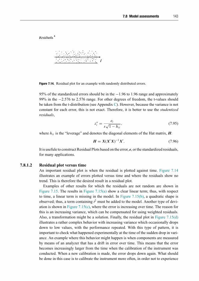
Trim: 247mm × 174mm Top: 12.653mm Gutter: 16.871mmCUUK2531-07 CUUK2531/Rasmuson ISBN: 978 1 107 04969 7 November 13, 2013 17:33
7.8 Model assessments 143
Figure 7.14. Residual plot for an example with randomly distributed errors.
95% of the standardized errors should be in the −1.96 to 1.96 range and approximately99% in the −2.576 to 2.576 range. For other degrees of freedom, the t-values shouldbe taken from the t-distribution (see Appendix C). However, because the variance is notconstant for each error, this is not exact. Therefore, it is better to use the studentizedresiduals,
z∗i = ei
s√
1 − hii, (7.95)
where hii is the “leverage” and denotes the diagonal elements of the Hat matrix, H:
H = X(X ′ X)−1 X ′. (7.96)
It is usefule to construct Residual Plots based on the error, e, or the standardized residuals,for many applications.
7.8.1.2 Residual plot versus timeAn important residual plot is when the residual is plotted against time. Figure 7.14illustrates an example of errors plotted versus time and where the residuals show notrend. This is therefore the desired result in a residual plot.
Examples of other results for which the residuals are not random are shown inFigure 7.15. The results in Figure 7.15(a) show a clear linear term; thus, with respectto time, a linear term is missing in the model. In Figure 7.15(b), a quadratic shape isobserved; thus, a term containing t2 must be added to the model. Another type of devi-ation is shown in Figure 7.15(c), where the error is increasing over time. The reason forthis is an increasing variance, which can be compensated for using weighted residuals.Also, a transformation might be a solution. Finally, the residual plot in Figure 7.15(d)illustrates a rather complex behavior with increasing variance which occasionally dropsdown to low values, with the performance repeated. With this type of pattern, it isimportant to check what happened experimentally at the time of the sudden drop in vari-ance. An example where this behavior might happen is when components are measuredby means of an analyzer that has a drift in error over time. This means that the errorbecomes increasingly larger from the time when the calibration of the instrument wasconducted. When a new calibration is made, the error drops down again. What shouldbe done in this case is to calibrate the instrument more often, in order not to experience

Trim: 247mm × 174mm Top: 12.653mm Gutter: 16.871mmCUUK2531-07 CUUK2531/Rasmuson ISBN: 978 1 107 04969 7 November 13, 2013 17:33
144 Statistical analysis of mathematical models
Figure 7.15. Residual plot versus time for examples with non-random errors.
Figure 7.16. Residual plot versus the regressor variable (Xi), where the errors are not random.
this problem. This example clearly shows that all trends observed in the residual plotsshould not be removed by adding new terms to the model. For some cases, there areexperimental problems, resulting in experiments having to be repeated or the experi-mental procedure refined, representing the causes of the trends in residual plots. It istherefore crucial for the person conducting the experiment to collaborate closely withthe model developer. There are many additional types of patterns that the residual plotscan assume; the objective of Figure 7.15 was to illustrate some of these patterns.
7.8.1.3 Residual plot versus xi
The residual can also be plotted versus each regressor variable (xi). These plots revealany missing trends in the model with respect to that regressor variable. The results shownin Figure 7.15(a) and (b) could also occur when plotting the residual versus xi, whichindicates that a linear or quadratic term in xi is missing. Another example is shown inFigure 7.16, where a sinusoidal term could be added.

Trim: 247mm × 174mm Top: 12.653mm Gutter: 16.871mmCUUK2531-07 CUUK2531/Rasmuson ISBN: 978 1 107 04969 7 November 13, 2013 17:33
7.8 Model assessments 145
Figure 7.17. Residual plot versus y calculated from the model, where the errors are not random.
Figure 7.18. Studentized residuals.
7.8.1.4 Residual plot versus yThe residual can also be plotted versus y calculated from the model. This type of residualplot is shown in Figure 7.17. The results show that the variance is increasing when thepredicted value increases. A reason for this may be that a lot of experimental analysisequipment has errors that are a percentage level of the maximum value, which means thatthe error increases when the value increases. Weighted residuals may represent a solutionto such a case, where the weights decrease as the y value increases. A transformation ofthe model might be another alternative.
7.8.1.5 OutliersOutliers are experimental points that deviate significantly from the others in the plot.This phenomenon was discussed in Section 7.4.2, and examples are shown in Figure 7.4and Figure 7.5. If the studentized residuals z∗
i are plotted, they should be in the –3 to3 range. However, if there are points larger than 3 or smaller than –3, they representoutliers. Figure 7.18 illustrates two outliers.
7.8.2 Analysis of variance (ANOVA) table
The variance can be analyzed in detail by using a so-called analysis of variance (ANOVA)table. An ANOVA table can be used (i) to determine whether a model is significant and

Trim: 247mm × 174mm Top: 12.653mm Gutter: 16.871mmCUUK2531-07 CUUK2531/Rasmuson ISBN: 978 1 107 04969 7 November 13, 2013 17:33
146 Statistical analysis of mathematical models
Table 7.1. Analysis of variance (ANOVA) table
Source SS df MS Fobs
Regression SSReg vReg M SReg = SSReg
vReg
M SReg
s2
Residual SSE v s2 = ss
v
lack of fit SSLoF vLoF M SLoF = SSLoF
vLoF
M SLoF
M SPE
Pure error SSPE vPE M SPE = SSPE
vPE
Total, corrected for mean SStot, corr vtot,corr
Figure 7.19. Data for three factors, showing differences within and between samples.
(ii) to check on its lack of fit. Repeated experiments are needed to examine this. Datafor three different factors (x1, x2, and x3) are shown in Figure 7.19. Each experimentis repeated multiple times in order to determine its variance. The figure shows that thevariance is larger for x2 than for the others because its points are more spread out. Themean value for y, y, is shown for the three factors. With the use of the ANOVA table,we can investigate if there is a lack of fit to the model. We can also examine whether thedifferences between yi are significant or are due to the variance of the points.
The ANOVA table is shown in Table 7.1; and in the following paragraph differentterms in the table and its use are discussed.
The first two lines represent the regression model and the residual, where the residualcan be divided into two parts: lack of fit and pure error. We start with the regression andresidual used to test if the model is significant. The sum of squares due to regression,SSReg, can be calculated according to
SSReg =n∑
i=1
(yi − y)2. (7.97)
This value is corrected to the mean, the background to subtracting the number ofparameters by one (for the mean) to retrieve the degrees of freedom:
vReg = p − 1, (7.98)

Trim: 247mm × 174mm Top: 12.653mm Gutter: 16.871mmCUUK2531-07 CUUK2531/Rasmuson ISBN: 978 1 107 04969 7 November 13, 2013 17:33
7.8 Model assessments 147
where p represents the number of parameters. The total sum of square errors, SSE, canbe calculated as described earlier as
SSE =m∑
i=1
e2i =
n∑i=1
(yi − yi )2, (7.99)
with
v = n − p (7.100)
degrees of freedom and
n =m∑
j=1
n j , (7.101)
where n represents the total number of observations and m is the number of different xi.For example, in the example in Figure 7.19, m = 3 and n = 6 + 5 + 6 = 17. The sumof square errors contains both the errors associated with the pure error, SSPE, and lackof fit SSLoF, i.e.
SSE = SSPE + SSLoF . (7.102)
The sum of squares of the pure error can be calculated from repeated identicalexperiments, according to
SSPE =m∑
j=1
n j∑i=1
(y ji − y j )2, (7.103)
with the number of degrees of freedom given by
vPE =m∑
j=1
(n j − 1) = n − m. (7.104)
The lack of fit of the model can be calculated via
SSLoF =m∑
j=1
n j (y j − y j )2, (7.105)
with
vLoF = m − p (7.106)
degrees of freedom. However, an easier way to determine SSLoF is to calculate it basedon Equation (7.102), resulting in
SSLoF = SSE − SSPE. (7.107)
Here, it becomes clear that the number of degrees of freedom for the lack of fit may becalculated from v and vPE:
vLoF = v − vPE = n − p − (n − m) = m − p. (7.108)

Trim: 247mm × 174mm Top: 12.653mm Gutter: 16.871mmCUUK2531-07 CUUK2531/Rasmuson ISBN: 978 1 107 04969 7 November 13, 2013 17:33
148 Statistical analysis of mathematical models
The total corrected sum of squares is given by
SStot,corr =n∑
i=1
(yi − y)2. (7.109)
It can also be calculated by adding the sum of squares for the regression and residual,which results in
SStot,corr = SSReg + SSE. (7.110)
It is referred to as “corrected” because it is corrected by the total mean, and this correctionis done in SSReg. Simultaneously, the degrees of freedom are corrected by –1 (due to themean), so
vtot,corr = n − 1. (7.111)
Dividing the sum of squares by the number of degrees of freedom for the respectivecase yields the, values for the mean squares, M SReg, s2, M SLoF , M SPE, M Stot,corr . Thepure error mean square, M SPE, is an estimate of σ 2 that is valid both when there is alack of fit in the model and when there isn’t.
The reason for setting up the ANOVA table is to determine if the model is significantand if there is any lack of fit to the model. First, we must determine if there is a lackof fit to the model. If there is, we cannot use s2 as an estimation of σ 2 and thus cannotcheck the significance of the model. The lack of fit can be determined by examining theobserved F-value for the lack of fit, that is
Fobs,LoF � M SLoF
M SPE. (7.112)
This value should be compared to the F-value from the F-distribution with vLoF
and vPE degrees of freedom at α confidence level (for example, at the 95% or the99% level), which is denoted F(vLoF, vPE; α). In the F-table (see Appendix C), dataare shown for F(v1, v2; α); thus v1 = vLoF and v2 = vPE. If Fobs,LoF > F(vLoF, vPE; α)is valid, the lack of fit is significant. For this case, it is not possible to determineconfidence regions, significance of the model, etc. Instead, residual plots and furtherexamination of the model are needed in order to uncover the reason for the lack of fit andthereafter to improve the model until there is no longer any lack of fit. For the case whenFobs,LoF < F(vLoF, vPE; α), there is no lack of fit observed and it becomes possible todetermine the significance of the model. In this case, we can use s2 as an estimation ofσ 2. However, the fact that there is no lack of fit does not mean that the model is perfect,it merely means that we do not observe any lack of fit in these analyses.
In order to examine the significance of the model, the F-value observed for theregression, Fobs,Reg, should be calculated:
Fobs,reg = M SReg
s2. (7.113)
This value should be compared to F(vReg, v; α) and if Fobs,Reg > F(vReg, v; α) is valid,the model is significant at the α level. However, if the opposite holds true, i.e. Fobs,Reg <
F(vReg, v; α), the model is not significant, and it is recommended not to use this model.
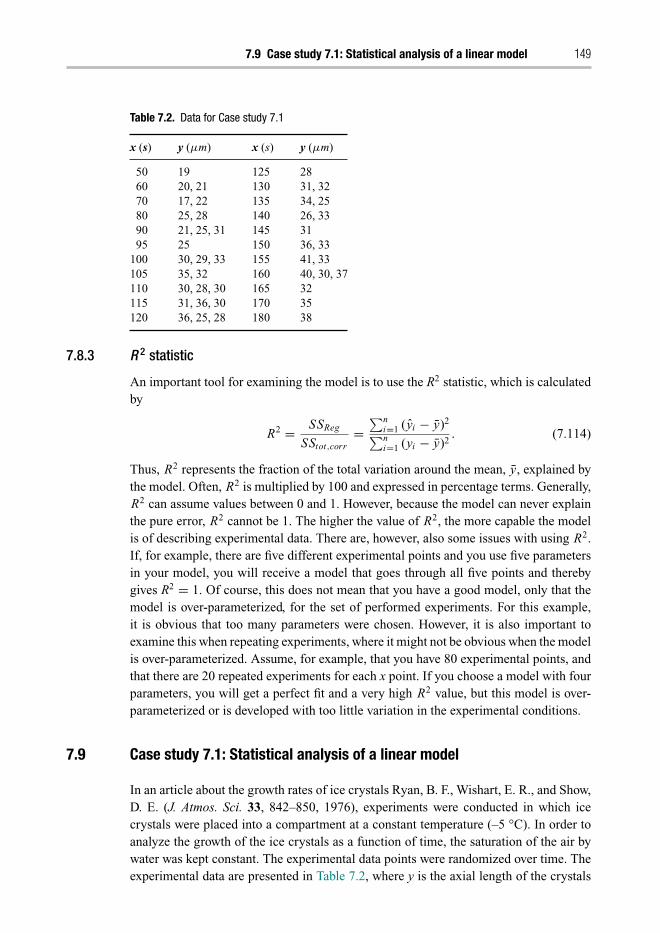
Trim: 247mm × 174mm Top: 12.653mm Gutter: 16.871mmCUUK2531-07 CUUK2531/Rasmuson ISBN: 978 1 107 04969 7 November 13, 2013 17:33
7.9 Case study 7.1: Statistical analysis of a linear model 149
Table 7.2. Data for Case study 7.1
x (s) y (μm) x (s) y (μm)
50 19 125 2860 20, 21 130 31, 3270 17, 22 135 34, 2580 25, 28 140 26, 3390 21, 25, 31 145 3195 25 150 36, 33
100 30, 29, 33 155 41, 33105 35, 32 160 40, 30, 37110 30, 28, 30 165 32115 31, 36, 30 170 35120 36, 25, 28 180 38
7.8.3 R 2 statistic
An important tool for examining the model is to use the R2 statistic, which is calculatedby
R2 = SSReg
SStot,corr=∑n
i=1 (yi − y)2∑ni=1 (yi − y)2
. (7.114)
Thus, R2 represents the fraction of the total variation around the mean, y, explained bythe model. Often, R2 is multiplied by 100 and expressed in percentage terms. Generally,R2 can assume values between 0 and 1. However, because the model can never explainthe pure error, R2 cannot be 1. The higher the value of R2, the more capable the modelis of describing experimental data. There are, however, also some issues with using R2.If, for example, there are five different experimental points and you use five parametersin your model, you will receive a model that goes through all five points and therebygives R2 = 1. Of course, this does not mean that you have a good model, only that themodel is over-parameterized, for the set of performed experiments. For this example,it is obvious that too many parameters were chosen. However, it is also important toexamine this when repeating experiments, where it might not be obvious when the modelis over-parameterized. Assume, for example, that you have 80 experimental points, andthat there are 20 repeated experiments for each x point. If you choose a model with fourparameters, you will get a perfect fit and a very high R2 value, but this model is over-parameterized or is developed with too little variation in the experimental conditions.
7.9 Case study 7.1: Statistical analysis of a linear model
In an article about the growth rates of ice crystals Ryan, B. F., Wishart, E. R., and Show,D. E. (J. Atmos. Sci. 33, 842–850, 1976), experiments were conducted in which icecrystals were placed into a compartment at a constant temperature (–5 °C). In order toanalyze the growth of the ice crystals as a function of time, the saturation of the air bywater was kept constant. The experimental data points were randomized over time. Theexperimental data are presented in Table 7.2, where y is the axial length of the crystals

Trim: 247mm × 174mm Top: 12.653mm Gutter: 16.871mmCUUK2531-07 CUUK2531/Rasmuson ISBN: 978 1 107 04969 7 November 13, 2013 17:33
150 Statistical analysis of mathematical models
in microns and x is the time in seconds. Repeated measurements were also performed inorder to examine the lack of fit.
Use a straight-line model, y = β0 + β1x + ε, and fit it to the data. In addition, makea complete statistical analysis of the model. Use a 95% confidence level, i.e. α = 0.05.
7.9.1 Solution
The experimental data are presented in vector and matrix notation:
y =
⎡⎢⎢⎢⎢⎢⎢⎢⎢⎢⎢⎢⎢⎢⎣
19202117···3538
⎤⎥⎥⎥⎥⎥⎥⎥⎥⎥⎥⎥⎥⎥⎦
X =
⎡⎢⎢⎢⎢⎢⎢⎢⎢⎢⎢⎢⎢⎢⎣
1 501 601 601 70· ·· ·· ·1 1701 180
⎤⎥⎥⎥⎥⎥⎥⎥⎥⎥⎥⎥⎥⎥⎦
where y is an n × 1 vector and X is an n × p matrix; n = 43 is the total number ofexperimental points, and p represents the number of parameters, in this case two (b0 andb1). The first column in X should only contain 1 at each position. The number of differentx-values is 22, which is denoted m (m = 22). As there are many repeated experiments,m is significantly lower than the total number of experimental points (n). The number ofobservations for each xi is named ni, where i = 1, . . . , m and n =∑m
i=1 ni .The model parameters can be calculated by as follows:
b =[
b0
b1
]= (X ′ X)−1 X ′ y =
[0.33355 −0.0026342
−0.0026342 2.23641 × 10⁻⁵
] [1292
158205
]=[
14.190.1346
].
Thus, the following model is obtained:
y = 14.19 + 0.1346x .
7.9.1.1 Evaluation of the modelWhen starting to evaluate the developed model, it is advisable to perform both regressionplots and residual plots. Figure 7.20 depicts a regression plot. Although the variance ishigh, the data follow the linear model closely. There are no clear trends or evidence ofoutliers.
Figures 7.21 and 7.22 show the residual and studentized residual versus the responsepredicted, respectively. These plots show that the residuals are evenly distributed andthat there are no clear trends. In the studentized residual plot (Figure 7.22), all pointsfall between −3 and 3, with no evidence of outliers (see Section 7.8.1).
As the residual plots evidence good behavior, we will proceed to assemble an ANOVAtable (Table 7.3) in order to study the lack of fit and the significance of the model (seeSection 7.8.2).

Trim: 247mm × 174mm Top: 12.653mm Gutter: 16.871mmCUUK2531-07 CUUK2531/Rasmuson ISBN: 978 1 107 04969 7 November 13, 2013 17:33
Figure 7.20. Regression plot.
Figure 7.21. Residual plot.
Figure 7.22. Studentized residual plot.

Trim: 247mm × 174mm Top: 12.653mm Gutter: 16.871mmCUUK2531-07 CUUK2531/Rasmuson ISBN: 978 1 107 04969 7 November 13, 2013 17:33
152 Statistical analysis of mathematical models
Table 7.3. ANOVA table for Case study 7.1
Source SS df MS Fobs
Regression 810.3 p − 1 = 2 − 1 = 1 810.3 63.45Residual 523.6 n − p = 43 − 2 = 41 12.77Lack of fit 239.6 m − p = 22 − 2 = 20 11.98 0.886Pure error 284 n − m = 43 − 22 = 21 13.52Total, corrected for the mean 1334 n − 1 = 43 − 1 = 42
7.9.1.2 Lack of fitThe lack of fit is examined by comparing Fobs to the F-value from the F-table (seeAppendix C), i.e.
F(vLoF, vPE; α) = F(20, 21; 0.005 = 2.1),
where the calculation for the degrees of freedom (df), for lack of fit (vLoF), and pureerror (vPE) are found in Table 7.3.
According to the calculation in the ANOVA table, Fobs,LoF = 0.886, which is smallerthan F(vLoF, vPE; α) = 2.1. Thus, the lack of fit is not significant and there is no reasonto doubt this model. We will therefore examine whether or not the regression model issignificant.
According to Table 7.3, the significance of the model is investigated by calculatingFobs,Reg = M SReg/s2 = 63.45. This value is compared with F(vReg, v; α), which becomesF(1; 41; 0.05) = 4.08 (see Table 7.3 for the calculation of the degrees of freedom).Thus, Fobs,Reg > F(vReg, v; α), which means that the model is significant at the α level.In addition, the R2 statistics is determined according to Equation (7.114), i.e.
R2 = SSReg
SStot,corr= 0.608.
Thus, the regression model describes a great deal of the variation in the data.
7.9.1.3 Confidence intervalsThe calculations of the confidence intervals are described in Section 7.5. Briefly, the1 − α confidence interval for the parameter bp in the model is given by
bp ± se(bp)t(n − p; α/2),where
se(bp) = s√
{(X ′ X)−1}pp;
s2 is already calculated and presented in the ANOVA table (Table 7.3). The confidenceintervals are presented in Table 7.4.
The confidence interval can also be written using the following notation:
10.02 ≤ β0 ≤ 18.36;
0.1005 ≤ β1 ≤ 0.1687.

Trim: 247mm × 174mm Top: 12.653mm Gutter: 16.871mmCUUK2531-07 CUUK2531/Rasmuson ISBN: 978 1 107 04969 7 November 13, 2013 17:33
7.10 Case study 7.2: Multiple regression 153
Table 7.4. Confidence intervals for Case study 7.1
Parameter bp se(bp) tobs Confidence interval
b0 14.19 2.064 6.875 14.19 ± 4.17b1 0.1346 0.0169 7.966 0.1346 ± 0.0341
Student’s t-tests can be used to determine the significance of the parameters. In order todo so, the t-value from the t-distribution is needed (see Appendix C):
t(n − p; α/2) = t(43 − 2; 0; 0.05/2) = 2.02.
This value should be compared with the calculated tobs = bp/se(bp), which are shownin the ANOVA table (Table 7.3). For both parameters tobs > 2.02, thus both parametersin the model are significant.
The confidence interval for the mean response, μ(x0), at x0 = 100, can be calculatedaccording to
y(x0) ± s√
x′0(X ′ X)−1x0 t(n − p; α/2),
resulting in
x0 = 27.65 ± 1.26,
26.4 ≤ μ(x0) ≤ 28.9.
7.9.1.4 CorrelationThe correlation coefficient can be determined by
C01 = {(X ′ X)−1}01√{(X ′ X)−1}00{(X ′ X)−1}11
= −0.9645.
The correlation is quite high.
7.10 Case study 7.2: Multiple regression
A die-casting process was examined and experiments conducted in order to study theeffects of the furnace temperature (x1) and the die-closing time (x2) on the temperaturedifference of the die surface (y). The data are shown in Table 7.5.
Fit the model y = β0 + β1x1 + β2x2 + ε to the data. In addition, make a completestatistical analysis of the model. Use a 95% confidence level, i.e. α = 0.05.

Trim: 247mm × 174mm Top: 12.653mm Gutter: 16.871mmCUUK2531-07 CUUK2531/Rasmuson ISBN: 978 1 107 04969 7 November 13, 2013 17:33
154 Statistical analysis of mathematical models
Table 7.5. Dataa for Case study 7.2
x1 x2 y
1250 6 801300 7 951350 6 1011250 7 851300 6 921250 8 871300 8 961350 7 1061350 8 108
See Chang, S. I. and Shivpuri, R.,Qual. Enging 7, 371–383, 1994.
7.10.1 Solution
The experimental data are presented below in vector and matrix notation:
y =
⎡⎢⎢⎢⎢⎢⎢⎢⎢⎢⎢⎢⎢⎢⎢⎢⎢⎣
80
95
101
85
92
87
96
106
108
⎤⎥⎥⎥⎥⎥⎥⎥⎥⎥⎥⎥⎥⎥⎥⎥⎥⎦
; X =
⎡⎢⎢⎢⎢⎢⎢⎢⎢⎢⎢⎢⎢⎢⎢⎢⎢⎣
1 1250 6
1 1300 7
1 1350 6
1 1250 7
1 1300 6
1 1250 8
1 1300 8
1 1350 7
1 1350 8
⎤⎥⎥⎥⎥⎥⎥⎥⎥⎥⎥⎥⎥⎥⎥⎥⎥⎦
,
where y is an n × 1 vector and X is an n × p matrix; n = 9 represents the total numberof experimental points, and p represents the number of parameters, in this case three(b0, b1, and b2). The first column of X should only contain 1 at each position. In theseexperiments, there are no repeated experimental points, and therefore the lack of fitcannot be determined.
The model parameters are given by:
b =⎡⎣b0
b1
b2
⎤⎦ = (X ′ X)−1 X ′ y
=⎡⎣120.94 −0.086667 −1.1667
−0.086667 6.6667 × 10⁻⁵ 5.1283 × 10⁻¹⁷
−1.1667 5.1283 × 10⁻¹⁷ 0.16667
⎤⎦⎡⎣850
11081505968
⎤⎦ =
⎡⎣−199.56
0.213.00
⎤⎦ .
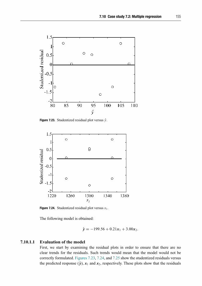
Trim: 247mm × 174mm Top: 12.653mm Gutter: 16.871mmCUUK2531-07 CUUK2531/Rasmuson ISBN: 978 1 107 04969 7 November 13, 2013 17:33
7.10 Case study 7.2: Multiple regression 155
Figure 7.23. Studentized residual plot versus y.
Figure 7.24. Studentized residual plot versus x1.
The following model is obtained:
y = −199.56 + 0.21x1 + 3.00x2.
7.10.1.1 Evaluation of the modelFirst, we start by examining the residual plots in order to ensure that there are noclear trends for the residuals. Such trends would mean that the model would not becorrectly formulated. Figures 7.23, 7.24, and 7.25 show the studentized residuals versusthe predicted response ( y), x1 and x2, respectively. These plots show that the residuals

Trim: 247mm × 174mm Top: 12.653mm Gutter: 16.871mmCUUK2531-07 CUUK2531/Rasmuson ISBN: 978 1 107 04969 7 November 13, 2013 17:33
156 Statistical analysis of mathematical models
Table 7.6. ANOVA table for Case stydy 7.2
Source SS df MS Fobs
Regression 715.5 p − 1 = 3 − 1 − 2 357.8 319.3Residual 6.72 n − p = 9 − 3 = 6 1.12Total, corrected for the mean 722.2 n − 1 = 9 − 1 = 8
Figure 7.25. Studentized residual plot versus x2.
are evenly distributed and that there are no clear trends. In addition, all points fallbetween −3 and 3, with no evidence of outliers (see Section 7.8.1).
Since the residual plots evidence good results, it is now possible to determine thesignificance of the model. See the ANOVA table (Table 7.6).
The significance of the model is examined by calculating Fobs,reg = M SReg/s2 =319.3 (see Table 7.6). The F-value can be retrieved from the F-table (see Appendix C)and F(vReg, v; α), which for this case study is F(2, 6; 0.05) = 5.14. This results inFobs,Reg > F(vReg,v; α), i.e. the model is significant at the α level. Further, the R2
statistic is determined using Equation (7.114) to be
R2 = SSReg
SStot,corr= 0.991.
Thus, we observe that the regression model can describe a large fraction of thevariation in the data.
7.10.1.2 Confidence intervalsThe calculations of the confidence intervals are discussed in Section 7.5. The 1 − α
confidence interval for the parameter bp in the model can be determined from
bp ± se(bp)t(n − p; α/2),
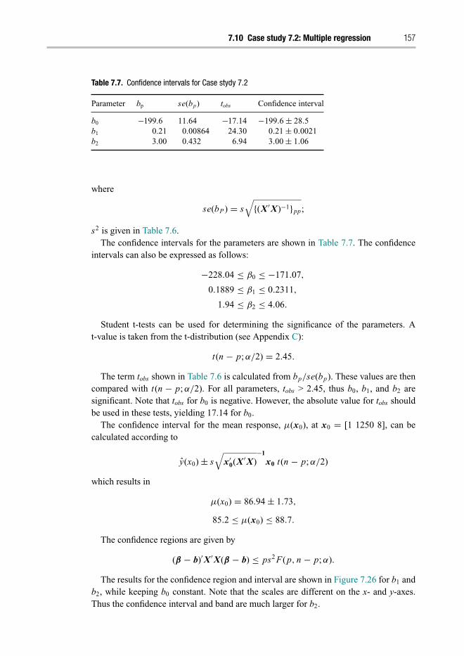
Trim: 247mm × 174mm Top: 12.653mm Gutter: 16.871mmCUUK2531-07 CUUK2531/Rasmuson ISBN: 978 1 107 04969 7 November 13, 2013 17:33
7.10 Case study 7.2: Multiple regression 157
Table 7.7. Confidence intervals for Case stydy 7.2
Parameter bp se(bp) tobs Confidence interval
b0 −199.6 11.64 −17.14 −199.6 ± 28.5b1 0.21 0.00864 24.30 0.21 ± 0.0021b2 3.00 0.432 6.94 3.00 ± 1.06
where
se(bP ) = s√
{(X ′ X)−1}pp;
s2 is given in Table 7.6.The confidence intervals for the parameters are shown in Table 7.7. The confidence
intervals can also be expressed as follows:
−228.04 ≤ β0 ≤ −171.07,
0.1889 ≤ β1 ≤ 0.2311,
1.94 ≤ β2 ≤ 4.06.
Student t-tests can be used for determining the significance of the parameters. At-value is taken from the t-distribution (see Appendix C):
t(n − p; α/2) = 2.45.
The term tobs shown in Table 7.6 is calculated from bp/se(bp). These values are thencompared with t(n − p; α/2). For all parameters, tobs ˃ 2.45, thus b0, b1, and b2 aresignificant. Note that tobs for b0 is negative. However, the absolute value for tobs shouldbe used in these tests, yielding 17.14 for b0.
The confidence interval for the mean response, μ(x0), at x0 = [1 1250 8], can becalculated according to
y(x0) ± s√
x′0(X ′ X)
−1
x0 t(n − p; α/2)
which results in
μ(x0) = 86.94 ± 1.73,
85.2 ≤ μ(x0) ≤ 88.7.
The confidence regions are given by
(β − b)′ X ′ X(β − b) ≤ ps2 F(p, n − p; α).
The results for the confidence region and interval are shown in Figure 7.26 for b1 andb2, while keeping b0 constant. Note that the scales are different on the x- and y-axes.Thus the confidence interval and band are much larger for b2.
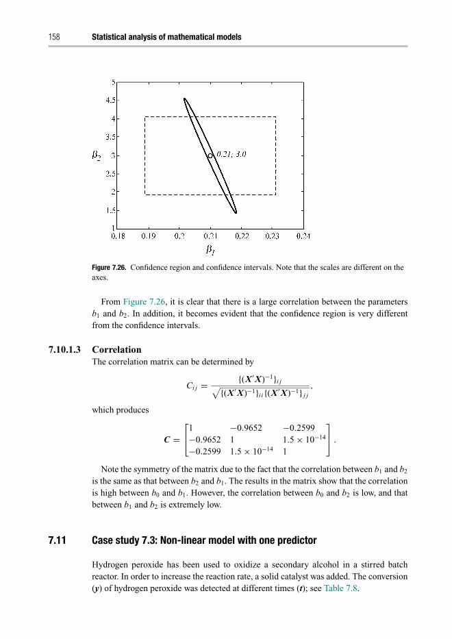
Trim: 247mm × 174mm Top: 12.653mm Gutter: 16.871mmCUUK2531-07 CUUK2531/Rasmuson ISBN: 978 1 107 04969 7 November 13, 2013 17:33
158 Statistical analysis of mathematical models
Figure 7.26. Confidence region and confidence intervals. Note that the scales are different on theaxes.
From Figure 7.26, it is clear that there is a large correlation between the parametersb1 and b2. In addition, it becomes evident that the confidence region is very differentfrom the confidence intervals.
7.10.1.3 CorrelationThe correlation matrix can be determined by
Ci j = {(X ′ X)−1}i j√{(X ′ X)−1}i i {(X ′ X)−1} j j
,
which produces
C =⎡⎣1 −0.9652 −0.2599
−0.9652 1 1.5 × 10⁻¹⁴
−0.2599 1.5 × 10⁻¹⁴ 1
⎤⎦ .
Note the symmetry of the matrix due to the fact that the correlation between b1 and b2
is the same as that between b2 and b1. The results in the matrix show that the correlationis high between b0 and b1. However, the correlation between b0 and b2 is low, and thatbetween b1 and b2 is extremely low.
7.11 Case study 7.3: Non-linear model with one predictor
Hydrogen peroxide has been used to oxidize a secondary alcohol in a stirred batchreactor. In order to increase the reaction rate, a solid catalyst was added. The conversion(y) of hydrogen peroxide was detected at different times (t); see Table 7.8.

Trim: 247mm × 174mm Top: 12.653mm Gutter: 16.871mmCUUK2531-07 CUUK2531/Rasmuson ISBN: 978 1 107 04969 7 November 13, 2013 17:33
7.11 Case study 7.3: Non-linear model with one predictor 159
Table 7.8. Data for Case study 7.3
t (min) y
20 0.047650 0.070080 0.129
110 0.152140 0.126170 0.157200 0.173230 0.140260 0.210290 0.155320 0.197
Table 7.9. ANOVA table for Case stydy 7.3
Source SS df MS Fobs
Regression 0.240 p = 2 0.12 244Residual 0.0044 n − p = 11 − 2 = 9 0.00049Total, corrected for the mean 0.244 n = 11
Fit the non-linear model y = θ1(1 − e−θ2 t ) to the data. Thereafter examine the sig-nificance of the model and the parameter significance. In addition, construct confidencebands and joint confidence regions. Use a 95% confidence level, i.e. α = 0.05.
7.11.1 Solution
The non-linear model parameters are determined numerically using the least squaremethod in Matlab. In order achieve this, the sum of square errors is used according to
SSE(θ ) =n∑
i=1
e2i =
n∑i=1
(yi − f (xi , θ ))2.
This results in the following parameters and model:
θ1 = 0.183, θ2 = 0.0122, and y = 0.183(1 − e−0.0122t ).
7.11.1.1 ANOVA tableThe ANOVA table is presented in Table 7.9. The reason that the degrees of freedomequal p not p − 1 is that this model does not contain a constant due to the mean (θ0).
The significance of the model is examined by comparing Fobs,Reg with F(vReg, v; α),which can be retrieved from the F-table. For this example, F(2, 9; 0.05) = 4.26 at the95% level. This results in Fobs,Reg > F(vReg, v; α), thus the model is significant at the α
level.

Trim: 247mm × 174mm Top: 12.653mm Gutter: 16.871mmCUUK2531-07 CUUK2531/Rasmuson ISBN: 978 1 107 04969 7 November 13, 2013 17:33
160 Statistical analysis of mathematical models
Table 7.10. Confidence intervals for Case stydy 7.3
Parameter θp se(θp) tobs Confidence interval
θ1 0.183 0.0147 12.43 0.183 ± 0.0333θ2 0.0122 0.00319 3.821 0.0122 ± 0.00723
7.11.1.2 Confidence intervals and bandsThe 1 − α confidence interval for the parameter θ p in the model can be determinedaccording to
θ p ± se(θ p)t(n − p; α/2),
where
se(θ p) = s√
{( J ′ J)−1}pp,
where J is the jacobian and can be calculated according to
Jn,p =[
∂ f (xn, θ )
∂θ p
]θ=θ
≈ f (xn, θ ) − (xn, θp,1%)
�θp
or directly through the software. In this case, MATLAB’s built-in functions have beenused to generate the Jacobian, resulting in
J(θ1, θ2) =
⎡⎢⎢⎢⎢⎢⎢⎢⎢⎢⎢⎢⎢⎢⎢⎢⎢⎢⎣
0.2166 2.86490.4568 4.96620.6234 5.50960.7388 5.25290.8189 4.63560.8744 3.90300.9129 3.18390.9396 2.53880.9581 1.99000.9710 1.53900.9799 1.1775
⎤⎥⎥⎥⎥⎥⎥⎥⎥⎥⎥⎥⎥⎥⎥⎥⎥⎥⎦
,
which yields
J ′ J =[
7.1627 27.260727.2607 151.8384
]
and
( J ′ J)−1 =[
0.4408 −0.0791−0.0791 0.0208
];
s2 is given in Table 7.9. The calculations for the confidence intervals are shown inTable 7.10.
The significance of the parameters is evaluated using the t-test. The t-valuet(n − p; α/2) is 2.26 (for the t-distribution, see Appendix C). Since the values of tobs for

Trim: 247mm × 174mm Top: 12.653mm Gutter: 16.871mmCUUK2531-07 CUUK2531/Rasmuson ISBN: 978 1 107 04969 7 November 13, 2013 17:33
7.11 Case study 7.3: Non-linear model with one predictor 161
Figure 7.27. Experimental data together with predicted conversion. In addition, the pointwise andcontinuous confidence bands are presented.
both parameters are larger than t(n − p; α/2), θ1 and θ2 are significant; tobs is calculatedusing tobs = bp/se(bp).
The 1 − α confidence interval for the dependent variable f (x0, θ ), which can also becalled the “mean response,” is retrieved by
f (x0, θ ) ± s√
j ′0( J ′ J)−1 j0 t(n − p; α/2),
where
j0 =[∂ f (x0, θ )
∂θ
]θ=θ
.
The confidence intervals for several points, calculated using the preceding equation,together form a so-called “1 − α pointwise confidence band”. The “simultaneous con-fidence band” at the 1 − α level is determined by
f (x, θ ) ± s√
j ′( J ′ J)−1 j√
pF(p; n − p; α).
The experimental data are shown in Figure 7.27 together with the predicted conversionusing the developed model. In addition, the resulting pointwise and simultaneousconfidence bands are shown. The results show that the pointwise and simultaneousconfidence bands are similar for this example.
7.11.1.3 Joint confidence regionsThe approximate elliptical contour, with exact probability level 1 − α, is calculatedusing
(θ − θ )′ × J ′ J × (θ − θ) ≤ ps2 F(p, n − p, 1 − α),

Trim: 247mm × 174mm Top: 12.653mm Gutter: 16.871mmCUUK2531-07 CUUK2531/Rasmuson ISBN: 978 1 107 04969 7 November 13, 2013 17:33
162 Statistical analysis of mathematical models
Figure 7.28. Confidence region and confidence intervals.
which yields
[θ1 − 0.1829 θ2 − 0.0122] × J ′ J ×[θ1 − 0.1829θ2 − 0.0122
]≤ 4 × 177 · 10−3.
The exact contour with approximate probability level 1 − α is determined using
s(θ) − s(θ ) ≤ ps2 F(p, n − p, 1 − α),
where
s(θ) = SSE.
The results for the confidence regions are shown in Figure 7.28, together with theindividual confidence intervals for θ1 and θ2. The results clearly show that there is alarge difference between the individual confidence intervals and the joint confidenceregions, but also that there is a difference between the elliptical contour and the exactregion. Further, the results of the joint confidence region also show that there is acorrelation between the parameters θ1 and θ2.
7.11.1.4 CorrelationThe correlation is determined using the correlation matrix according to
Ci j = {( J ′ J)−1}√{( J ′ J)−1}i i {( J ′ J)−1} j j
,
which gives
C =[
1 −0.8266−0.8266 1
].
Thus, there is a quite high correlation between the parameters.

Trim: 247mm × 174mm Top: 12.653mm Gutter: 16.871mmCUUK2531-07 CUUK2531/Rasmuson ISBN: 978 1 107 04969 7 November 13, 2013 17:33
7.13 Practice problems 163
7.12 Questions
(1) Set up the normal equations and derive expressions for b0 and b1 in a linearmodel.
(2) How can the parameters in vector b be determined using the matrix form?
(3) Why are weighted residuals used?
(4) What is an outlier?
(5) How do you determine confidence intervals and regions, respectively?
(6) What are the differences between confidence intervals and confidence bands?
(7) Describe the ANOVA table and how to calculate the different values in the table.
(8) What is the correlation between parameters and how do you determine it?
(9) Why is the correlation matrix symmetrical?
(10) What makes a model non-linear?
(11) Give an example of an intrinsically linear model.
(12) How do you determine confidence intervals for a non-linear model?
(13) Give examples of residual plots when the residuals are evenly distributed and whenthere are clear trends. Also describe how the models should be changed when cleartrends are discernible.
(14) How is R2 determined in order to get information about how much of a variationcan be described by a model?
7.13 Practice problems
7.1 The dependence of the reaction rate for the pressure of a hydrogenation reaction ina tubular reactor has empirically been shown to follow the model
r(P) = θ1 · P
1 + θ2 · P
where r is the reaction rate (mol s−1, per kilogram of catalyst) and P is the totalpressure (bar). At 170 °C, the reaction rates given in Table 7.11 were determined.(a) Determine the parameters θ1 and θ2 by using one of Matlab’s (or that of another
software) least square functions to search for the parameter values that minimizethe model error. In order to obtain a rapid convergence against the global minima,good start guesses of θ1 and θ2 are important.
(b) Determine the individual confidence intervals for the parameters at a 95%level.

Trim: 247mm × 174mm Top: 12.653mm Gutter: 16.871mmCUUK2531-07 CUUK2531/Rasmuson ISBN: 978 1 107 04969 7 November 13, 2013 17:33
164 Statistical analysis of mathematical models
Table 7.11. Reaction rates as a function ofpressure
r (mol s−1 per kg catalyst) P (bar)
0.0192 1.3820.0234 2.0750.0258 2.4310.0281 2.7620.0318 3.5000.0319 3.8330.0334 4.129
Table 7.12. Reaction rates for the two cases treated and untreated withpyromycin
Reaction rate (counts/min2)
Substrate concentration (ppm) Treated with pyromycin Untreated
0.025 79 690.025 45 550.07 94 870.07 111 810.105 127 1010.105 142 1110.23 163 1290.23 156 1270.54 194 1420.54 199 1591.18 209 1621.18 205 161
(c) Plot the joined, approximate confidence region of the parameters at the 95%level. Hint: If you use Matlab, the contour function can be a great help.
(d) Determine the prediction interval for a new observation at 2.8 bar pressure.
7.2 The possible effect the substance pyromycin might have on an enzymatic reactionis examined. Two experimental series are conducted, one applying the pyromycintreatment, the other without. In the tests, the dependence of the reaction rate onthe substrate concentration is measured. The kinetics can be assumed to follow theMichaelis–Menten model:
f (θ, x) = θ1 · x
θ2 + x.
An hypothesis is that pyromycin influences parameter θ1, not θ2. Do a statisticalanalysis and, based on that result, determine whether the hypothesis is likely to betrue or not. The experimental data are given in Table 7.12.

Trim: 247mm × 174mm Top: 12.653mm Gutter: 16.871mmCUUK2531-07 CUUK2531/Rasmuson ISBN: 978 1 107 04969 7 November 13, 2013 17:33
7.13 Practice problems 165
Table 7.13. Data for pressure drop, pressure, heat loading and mass flow
Measured Calculated Absolute Heatpressure drop pressure drop pressure loading Mass flow(kPa m−1) (kPa m−1) (kPa) (kW m−2) (kg m−2 s−1)
1.440 1.188 296.9 3.64 3162.174 1.731 296.0 19.35 2011.193 0.758 292.9 14.65 1251.602 1.585 594.7 3.24 3162.545 2.849 595.8 18.96 2011.204 1.251 594.0 6.42 1250.989 1.093 792.6 3.35 3162.765 3.072 795.6 7.56 2010.791 0.984 784.4 11.55 125
(a) Determine the parameters θ1 and θ2 by non-linear regression.(b) Determine the individual 95% confidence intervals of the parameters. Are the
parameters correlated; if your answer is yes, how?(c) Conduct a residual analysis using studentized residuals.(d) Determine if there are any significant model errors (lack of fit).(e) Perform the corresponding analysis for the untreated series.(f) Based on these results, what do you think of the stated hypothesis?
7.3 A PhD student at Chalmers University measured the pressure drop during evapora-tion of 1,1,1,2-tetrafluoroetan in tubes. The student also calculated what a certainmodel, in the form of pressure drop = f (pressure, heat loading, mass flow), wascapable of predicting for the same conditions. The conditions and results are shownin Table 7.13.
Examine, with the help of residual analysis, if there is reason to suspect thatthe model needs further development, and, if so, in what regard. Normalization orstudentization is not needed.
7.4 When conducting a lack of fit analysis, the following ratio:
SSLoF/vLoF
SPE/vPE,
is compared with the F-distribution value for F(v1, vPE, α). In Figure 7P.1, thereaction rate is given as a function of reactant concentration. The points representexperimentally measured values, and the solid line represents a model with twoparameters. There are 29 points in total. For the five highest concentrations, repeatedexperiments are taking place.(a) Which contribution to SSRes (the residual sum of squares), SSLoF, respectively
SSPE, originates from the two points between the concentrations 0.4 and 0.6?Illustrate graphically the differences that form the basis for SSRes and SPE.
(b) What is the F-distribution value at the 95% level for the example in Figure P7.1?(c) What does it mean if the ratio becomes larger than the F-distribution value?

Trim: 247mm × 174mm Top: 12.653mm Gutter: 16.871mmCUUK2531-07 CUUK2531/Rasmuson ISBN: 978 1 107 04969 7 November 13, 2013 17:33
166 Statistical analysis of mathematical models
Table 7.14. Input data for the model
N T C Yobs Ycalculated Res
1 285 7 2.3 2.94 –0.642 254 7 3.2 3.50 –0.33 302 9 3.0 2.57 0.434 323 6 1.6 2.23 –0.635 314 10 2.4 2.41 –0.016 282 8.5 3.7 2.95 0.757 321 5.3 1.4 2.26 –0.868 302 10 3.5 2.61 0.899 324 11.5 2.7 2.26 0.44
Figure P7.1. Reaction rate as a function of reactant concentration.
7.5 In order to reduce the shrinkage of an artificial fiber, it is pretreated by dipping intoa solution with concentration C and then heat-treated at temperature T. The goal isto make a model describing how the shrinkage Y depends on the pretreatment.
Nine experiments were conducted; the data are shown in Table 7.14. The measuredshrinkage is denoted Yobs. The results of a first version of the model is also givenin the column YCalculated. Note that N is the notation for the experiment number, andthe residual is denoted “Res”.
With the help of residual analysis, examine the suggested model and suggest, withmotivation, if and how the model might be improved.
7.6 As part of an assignment to find the optimal process conditions in a steam stripper,a simple model is needed. The model should describe how the water content in the

Trim: 247mm × 174mm Top: 12.653mm Gutter: 16.871mmCUUK2531-07 CUUK2531/Rasmuson ISBN: 978 1 107 04969 7 November 13, 2013 17:33
7.13 Practice problems 167
Table 7.15. Water content in the distillate
x (kg s−1) y
0.263 0.340.294 0.320.321 0.240.367 0.200.429 0.160.608 0.111.33 0.06
13.6 0.04
distillate (y) depends on the steam consumption (x). As a basis for the model, thedata in Table 7.15 were collected during the experiments.
The following model is suggested:
y = a(
ln( x
b
))−2/3,
where a and b are the parameters in the model.By minimizing the residual sum of squares, SSE, the following data were obtained:
� a (parameter 1) = 0.1321� b (parameter 2) = 0.2110 kg s−1
� SSE = 0.003726
� J T J =[
20.3453 25.925425.9254 38.9143
]
� ( J T J)−1 =[
0.3254–0.2168−0.2168 0.1701
](a) Optimal steam flow is expected to be about 0.58 kg s−1. Calculate a 95%
confidence interval, which will describe the uncertainty of the model for thisflow.
(b) Others that have conducted similar experiments have found a = 0.107 and b =0.211. Are these parameters on the 95% significance level?

Trim: 247mm × 174mm Top: 12.653mm Gutter: 16.871mmCUUK2531-APP-A CUUK2531/Rasmuson ISBN: 978 1 107 04969 7 November 13, 2013 9:42
Appendix AMicroscopic transport equations
A.1 Rectangular coordinates
Mass balance for component A (ρ and DAB constant)
∂CA
∂t+ vx
∂CA
∂x+ vy
∂CA
∂y+ vz
∂CA
∂z= DAB
(∂2CA
∂x2+ ∂2CA
∂y2+ ∂2CA
∂z2
)+ RA.
Total mass balance (ρ constant)
∂vx
∂x+ ∂vy
∂y+ ∂vz
∂z= 0.
Energy balance (ρ and k constant)
ρcp
(∂T
∂t+ vx
∂T
∂x+ vy
∂T
∂y+ vz
∂T
∂z
)= k
(∂2T
∂x2+ ∂2T
∂y2+ ∂2T
∂z2
)+ S.
Momentum balance (ρ and μ constant)
x : ρ
(∂vx
∂t+ vx
∂vx
∂x+ vy
∂vx
∂y+ vz
∂vx
∂z
)= −∂p
∂x+ μ
(∂2vx
∂x2+ ∂2vx
∂y2+ ∂2vx
∂z2
)+ ρgx ,
y : ρ
(∂vy
∂t+ vx
∂vy
∂x+ vy
∂vy
∂y+ vz
∂vy
∂z
)= −∂p
∂y+ μ
(∂2vy
∂x2+ ∂2vy
∂y2+ ∂2vy
∂z2
)+ ρgy,
z : ρ
(∂vz
∂t+ vx
∂vz
∂x+ vy
∂vz
∂y+ vz
∂vz
∂z
)= −∂p
∂z+ μ
(∂2vz
∂x2+ ∂2vz
∂y2+ ∂2vz
∂z2
)+ ρgz .
A.2 Cylindrical coordinates (mass and energy)
Mass balance for component A (ρ and DAB constant)
∂CA
∂t+ vr
∂CA
∂r+ vθ
1
r
∂CA
∂θ+ vz
∂CA
∂z= DAB
(1
r
∂
∂rr∂CA
∂r+ 1
r2
∂2CA
∂θ2+ ∂2CA
∂z2
)+ RA.

Trim: 247mm × 174mm Top: 12.653mm Gutter: 16.871mmCUUK2531-APP-A CUUK2531/Rasmuson ISBN: 978 1 107 04969 7 November 13, 2013 9:42
Microscopic transport equations 169
Energy balance (ρ and k constant)
ρcp
(∂T
∂t+ vr
∂T
∂r+ vθ
1
r
∂T
∂θ+ vz
∂T
∂z
)= k
(1
r
∂
∂rr∂T
∂r+ 1
r2
∂2T
∂θ2+ ∂2T
∂z2
)+ S.
A.3 Spherical coordinates (mass and energy)
Mass balance for component A (ρ and DAB constant)
∂CA
∂t+ vr
∂CA
∂r+ vθ
1
r
∂CA
∂θ+ vϕ
1
r sin θ
∂CA
∂ϕ
= DAB
(1
r2
∂
∂rr2 ∂CA
∂r+ 1
r2 sin θ
∂
∂θsin θ
∂CA
∂θ+ 1
r2 sin2 θ
∂2CA
∂ϕ2
)+ RA.
Energy balance (ρ and k constant)
ρcp
(∂T
∂t+ vr
∂T
∂r+ vθ
1
r
∂T
∂θ+ vϕ
1
r sin θ
∂T
∂ϕ
)
= k
(1
r2
∂
∂rr2 ∂T
∂r+ 1
r2 sin θ
∂
∂θsin θ
∂T
∂θ+ 1
r2 sin2 θ
∂2T
∂ϕ2
)+ S.

Trim: 247mm × 174mm Top: 12.653mm Gutter: 16.871mmCUUK2531-APP-B CUUK2531/Rasmuson ISBN: 978 1 107 04969 7 November 13, 2013 14:13
Appendix BDimensionless variables
Useful dimensionless numbers can be created by taking the ratios of different forces,mass fluxes, or heat fluxes. The dimensionless number will indicate which of theforces or fluxes is the most important. Various dimensionless quantities are given inTables B.1–B.4.
Table B.1. Dimensionless numbers based on force
Inertial Viscous Buoyancy Surface tension Pressure
Force (kg m s−2) ρU 2 L2 μU L gL3�ρ γ L L2�p
Inertial – Re = ρUL
μFr = gL�ρ
ρU 2We = ρU 2 L
γEu = �p
ρU 2
Viscous –gL2�ρ
μUCa = μU
γ
L�p
μU
Buoyancy – Eo = gL2�ρ
γ
�p
gL�ρ
Surface tension –L�p
γPressure –
Table B.2. Dimensionless numbers based on mass flux
Convective Diffusion Interface Reaction
Mass flux (mol s−1) U�C L2 D�C L kw�C L2 rA L3
Convective – Pe = U L
DSt = kw
UDaI = LrA
U�C
Diffusive – Sh = kw L
DDaI I = L2rA
D�C
Interface –rA L
kw�C
Reaction –

Trim: 247mm × 174mm Top: 12.653mm Gutter: 16.871mmCUUK2531-APP-B CUUK2531/Rasmuson ISBN: 978 1 107 04969 7 November 13, 2013 14:13
Dimensionless variables 171
Table B.3. Dimensionless numbers based on heat flux
Convective Conductive Interphase Reaction
Heat flux (J s−1) ρCp�T U L2 k�T L h�T L2 rA L3�H
Convective – Pe = ρcpU L
kSt = h
cpρUDaI I I = rA L�H
ρcpU�T
Conductive – Nu = hL
kDaI V = rA�H L2
k�T
Interphase –rA L�H
h�T
Reaction –
Table B.4. Common dimensionless numbers
Name Definition
Biot Bi = hL
k
external heat transfer
internal conductive heat transfer
Capillary Ca = μU
γ
viscous force
capillay force
Damkohler I Da = knCn0
C0U/L= knCn−1
0 τreaction rate
convective mass transport rate
Damkohler II DaI I = knCn−10
kga
reaction rate
mass transport rate
Damkohler III DaI I = knCn−10 L�H
ρcpU�T
heat of reaction
heat transport rate
Eotvos Eo = gL2�ρ
γ
buoyancy force
surface tension force
Euler Eu = �p
ρU 2
pressure force
inertia force
Fourier Fo = αt
L2
heat conduction
heat accumulation
Froude Fr = gL�ρ
ρU 2
buoyed weight
surface inertia force
Grashof Gr = ρ2gβ(Ts − T∞)L3
μ2
(buoyancy) (inertia force)
viscous force
Nusselt Nu = hL
k
convective heat transfer
conductive heat transfer
Peclet PeH = LU
αorPeD= LU
D
convective transport
diffusive transport
Prandtl Pr = μ
ρα
viscosity
heat diffusivity
Rayleigh Ra = ρgβ(Ts − T∞)L3
μα
free convection
conduction(cont.)
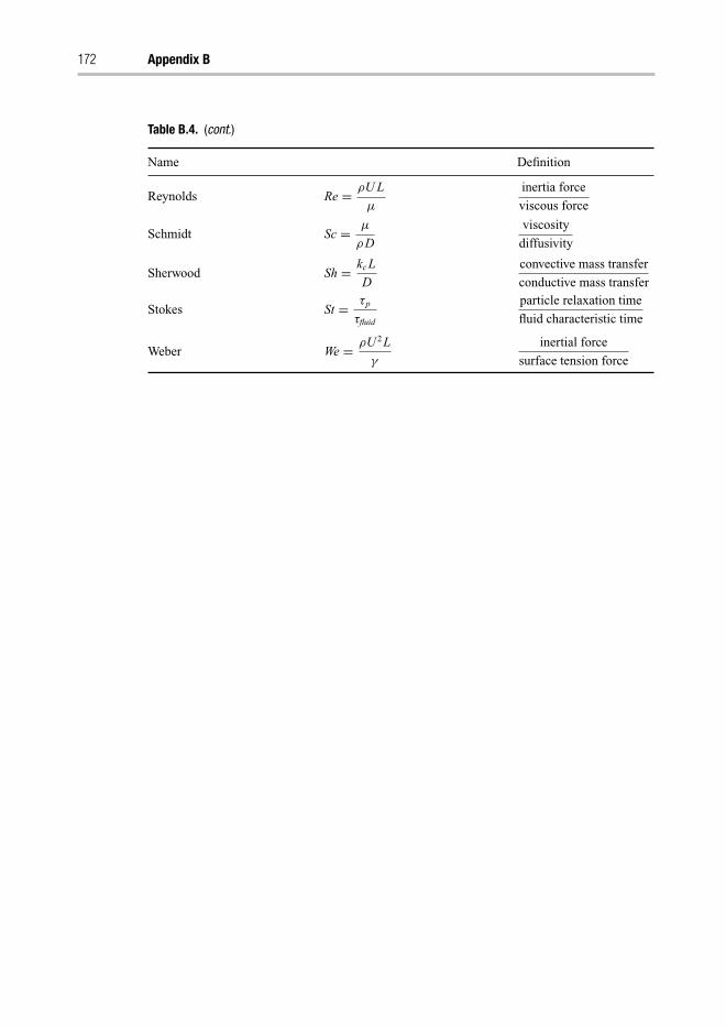
Trim: 247mm × 174mm Top: 12.653mm Gutter: 16.871mmCUUK2531-APP-B CUUK2531/Rasmuson ISBN: 978 1 107 04969 7 November 13, 2013 14:13
172 Appendix B
Table B.4. (cont.)
Name Definition
Reynolds Re = ρU L
μ
inertia force
viscous force
Schmidt Sc = μ
ρD
viscosity
diffusivity
Sherwood Sh = kc L
D
convective mass transfer
conductive mass transfer
Stokes St = τp
τfluid
particle relaxation time
fluid characteristic time
Weber We = ρU 2 L
γ
inertial force
surface tension force

Trim: 247mm × 174mm Top: 12.653mm Gutter: 16.871mmCUUK2531-APP-C CUUK2531/Rasmuson ISBN: 978 1 107 04969 7 November 13, 2013 15:14
Appendix CStudent’s t-distribution
Table C.1. t-table
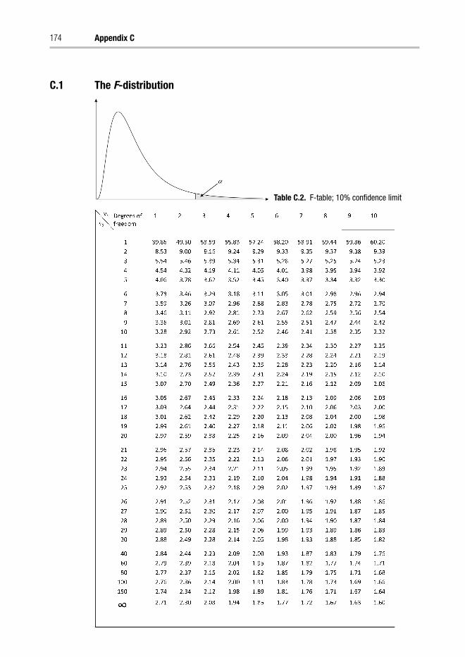
Trim: 247mm × 174mm Top: 12.653mm Gutter: 16.871mmCUUK2531-APP-C CUUK2531/Rasmuson ISBN: 978 1 107 04969 7 November 13, 2013 15:14
174 Appendix C
C.1 The F-distribution
Table C.2. F-table; 10% confidence limit

Trim: 247mm × 174mm Top: 12.653mm Gutter: 16.871mmCUUK2531-APP-C CUUK2531/Rasmuson ISBN: 978 1 107 04969 7 November 13, 2013 15:14
Student’s t-distribution 175
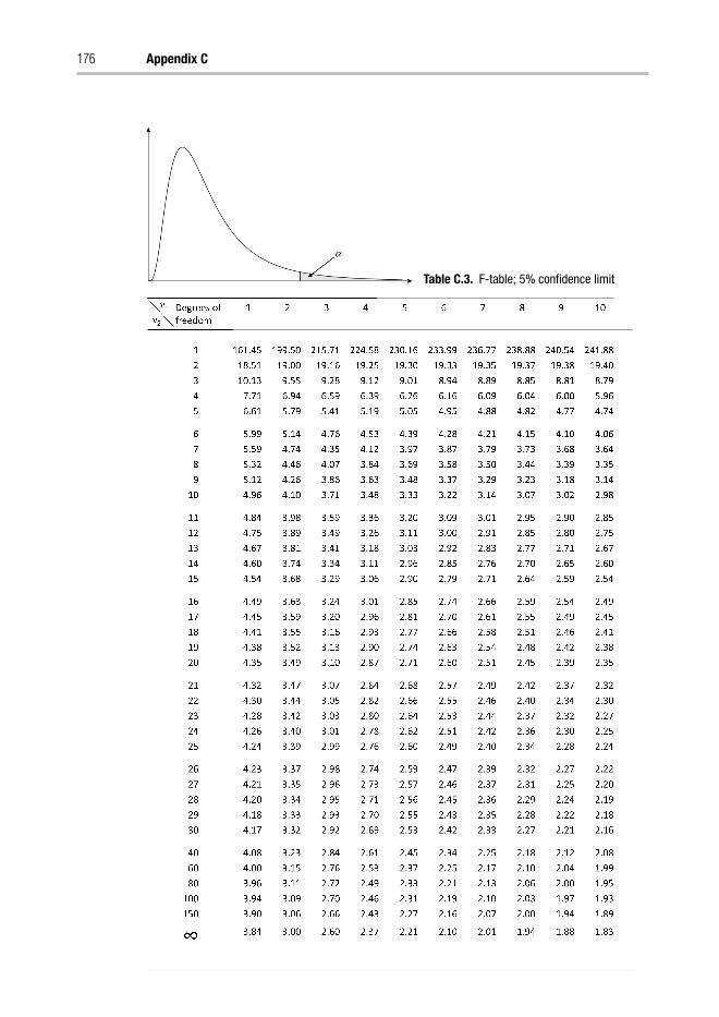
Trim: 247mm × 174mm Top: 12.653mm Gutter: 16.871mmCUUK2531-APP-C CUUK2531/Rasmuson ISBN: 978 1 107 04969 7 November 13, 2013 15:14
176 Appendix C
Table C.3. F-table; 5% confidence limit

Trim: 247mm × 174mm Top: 12.653mm Gutter: 16.871mmCUUK2531-APP-C CUUK2531/Rasmuson ISBN: 978 1 107 04969 7 November 13, 2013 15:14
Student’s t-distribution 177

Trim: 247mm × 174mm Top: 12.653mm Gutter: 16.871mmCUUK2531-APP-C CUUK2531/Rasmuson ISBN: 978 1 107 04969 7 November 13, 2013 15:14
178 Appendix C
Table C.4. F-table; 1% confidence limit

Trim: 247mm × 174mm Top: 12.653mm Gutter: 16.871mmCUUK2531-APP-C CUUK2531/Rasmuson ISBN: 978 1 107 04969 7 November 13, 2013 15:14
Student’s t-distribution 179

Trim: 247mm × 174mm Top: 12.653mm Gutter: 16.871mmCUUK2531-FR CUUK2531/Rasmuson ISBN: 978 1 107 04969 7 November 13, 2013 15:22
Bibliography
Bird, R.B., W.E. Stewart, and E.N. Lightfoot, Transport Phenomena, 2nd edn. New York: Wiley,2002.
Levenspiel, O., Chemical Reaction Engineering, 3rd edn. New York: Wiley, 1999.Welty, J.R., C.E. Wicks, and R.E. Wilson, Fundamentals of Momentum, Heat and Mass Transfer,
5th edn. Hoboken, NJ: Wiley, 2007.Kunes, J., Dimensionless Physical Quantities in Science and Engineering. Burlington, MA:
Elsevier, 2012.LeVeque, R.J., Finite Difference Methods for Ordinary and Partial Differential Equations: Steady-
State and Time-Dependent Problems. Philadelphia, PA: SIAM, 2007.Sauer, T., Numerical Analysis. Boston, MA: Pearson, 2012.Haberman, R., Applied Partial Differential Equations. Upper Saddle River, NJ: Pearson, 2004.Draper, N.R. and H. Smith, Applied Regression Analysis, 3rd edn. New York: John Wiley & Sons,
1998.Chatfield, C., Statistics for Technology, 3rd edn. London: Chapman and Hall, 1983.Mendenhall, W. and T. Sincich, A Second Course in Statistics Regression Analysis, 6th edn. Upper
Saddle River, NJ: Pearson Education International, 2003.Devore, J. and N. Farnum, Applied Statistics for Engineers and Scientists, 2nd edn. Belmont, CA:
Thomson, 2005.Montgomery, D.C., Design and Analysis of Experiments, 7th edn. Hoboken, NJ: John Wiley &
Sons, 2009.

Trim: 247mm × 174mm Top: 12.653mm Gutter: 16.871mmCUUK2531-IND CUUK2531/Rasmuson ISBN: 978 1 107 04969 7 November 13, 2013 18:50
Index
accumulation, 23accuracy, 88Adams–Bashforth method, 93Adams–Moulton method, 94, 97adaptive step size, 88ANOVA table, 145, 146, 152, 156approximate confidence interval, 140averaging, 54
backward difference, 113backward differentiation formulas, 97balance, 20
component, 21energy, 21mass, 20momentum, 22
base dimensions, 40boundary conditions, 26, 54, 67boundary-value problem, 82, 99Buckingham’s � theorem, 48
central differences, 103, 110characteristic variables, 44circulation time, 51collocation, 107collocation points, 107conditional stability, 90conduction, 23confidence band, 135, 136, 141, 161confidence interval, 130, 152, 156, 162
for the dependent variable, 135confidence region, 135, 141, 157, 162conservation, 20constitutive equation, 22
Darcy, 22Fick, 22Fourier, 22Newton, 22
continuous variable, 11control volume, 24correlation, 40, 136, 142, 153, 158, 162correlation matrix, 136, 137, 142coupling, 14Crank–Nicolson method, 114
decoupling, 54, 55, 72degrees of freedom, 130, 131dependent variable, 121deterministic model, 13diffusion, 24dimensionless equations, 41, 43dimensionless number
Euler, 43Froude, 43Peclet, 43Prandtl, 43Reynolds, 43Schmidt, 43
dimensionless variable, 40, 46Dirichlet boundary condition, 103discrete variable, 11distributed parameter, 11Dormand–Prince method, 89
elliptic PDE, 110empirical model, 14, 40, 46error, 53
global, 87local, 87
error control, 89error estimation, 76error tolerance, 98explicit algorithms, 87explicit Euler method, 82extrapolation, 13
F-distribution, 135fictitious boundary, 104, 106film theory, 45finite difference method, 102, 110finite element method, 107first-order derivative, 64flow, 24flux, 22forward difference, 110Frossling correlation, 46
Gaussian elimination, 103, 106grid, 102

Trim: 247mm × 174mm Top: 12.653mm Gutter: 16.871mmCUUK2531-IND CUUK2531/Rasmuson ISBN: 978 1 107 04969 7 November 13, 2013 18:50
182 Index
Hagen–Poiseuille equation, 44heat transfer, 44, 46higher-order differential equations, 96hydraulic diameter, 57hyperbolic PDE, 110
implicit Euler method, 91implicit methods, 90independent variable, 54, 69, 121initial-value problem, 82interpolation, 13intrinsically linear models, 138
Jacobian, 140
lack of fit, 146, 147, 148, 152least square method, 123, 126limiting cases, 54, 63linear model, 10linear regression, 121, 122, 125linearizing, 54, 61local truncation error, 83, 87lumped parameter, 11lumping, 56
MATLAB, 114mechanistic model, 14mesh, 102micromixing, 51midpoint method, 84mirror planes, 56mixing, 50multistep methods
explicit, 93implicit, 94
neglecting terms, 54, 64Neumann boundary condition, 104Newton method, 93non-linear model, 10, 123, 139, 159non-recurring set, 47normal equation, 124numerical differentiation formulas, 97
Octave, 117ordinary differential equation, 81outlier, 129, 145over- and underestimation, 77
parabolic PDE, 110partial differential equations, 108periodic boundary condition, 56polynomial model, 122population balance, 28predictor, 121predictor–corrector pairs, 94
primary dimensions, 46pumping capacity, 51pure error, 146, 147
R2 statistic, 149random error, 132Ranz–Marshall correlation, 46rate determining, 50rate of dissipation, 51reaction time, 50recurring set, 47regressor, 121residence time distribution, 32residual plots, 142, 143, 144response variable, 121Runge–Kutta method, 86Runge–Kutta–Fehlberg method, 89
scalemacroscopic, 18mesoscopic, 17microscopic, 16molecular, 16
scale-independent model, 49scaling down, 48scaling out, 48scaling rule, 51scaling up, 48second-order derivative, 64sensitivity analysis, 77shell balance, 23shooting method, 99simplified geometry, 54stability, 90, 91standard error, 130steady state, 11, 54, 58, 60, 70stencil, 111stiff problems, 97stochastic model, 13straight-line model, 121, 123, 131Student’s t-distribution, 133studentized residual, 150sum of square error, 123, 124, 126, 130, 147symmetry, 55, 56, 69system of differential equations, 94
Taylor expansion, 62, 83t-distribution, 135time constants, 58time scales, 97total corrected sum of squares, 148transformation, 96transient model, 11, 54, 58transport phenomena, 22trial function, 107truncation error, 87

Trim: 247mm × 174mm Top: 12.653mm Gutter: 16.871mmCUUK2531-IND CUUK2531/Rasmuson ISBN: 978 1 107 04969 7 November 13, 2013 18:50
Index 183
t-tests of individual parameters, 133turbulent eddies, 51turbulent kinetic energy, 51
uncertainty, 53unconditional stability, 91unsteady state, 58
validation, 53variance, 125, 127, 136verification, 53
weighted least squares, 127weighted sum of square error,
129

Trim: 247mm × 174mm Top: 12.653mm Gutter: 16.871mmCUUK2531-IND CUUK2531/Rasmuson ISBN: 978 1 107 04969 7 November 13, 2013 18:50