MIT OpenCourseWare http://ocw.mit.edu

16.89J / ESD.352J Space Systems Engineering Spring 2007

For information about citing these materials or our Terms of Use, visit: http://ocw.mit.edu/terms.

?

Critical Design Review

Terrestrial Planet Finder Mission

Massachusetts Institute of Technology Department of Aeronautics and Astronautics

16.89 - Space Systems Engineering

May 10, 1999

Formal Presentation 16.89 Space Systems Engineering

CRITICAL DESIGN REVIEW 10 May 1999

The Terrestrial Planet Finder Mission Development of a Quantitative Systems Engineering Methodology

Graduate Curriculum

Department of Aeronautics and Astronautics

Massachusetts Institute of Technology

77 Massachusetts Avenue

Cambridge, MA 02139, U.S.A.

1

CDR PresentatCDR Presenta ion Outlinetion Outline

1. Introduction and Motivation1. Introduction and Motivation2. Systems Engineering Process2. Systems Engineering Process3. TPF Mission Analysis Software3. TPF Mission Analysis Software4. Interactive Test Case4. Interactive Test Case5. TPF Mission Trade Studies5. TPF Mission Trade Studies6. Conclusions6. Conclusions7. Question and Answer Session7. Question and Answer Session

Presented by : Olivier de Weck, Troy Hacker, Sangwoo PakPresented by : Olivier de Weck, Troy Hacker, Sangwoo Pak

This slide shows the outline of the presentation. Sections 1 and 2 show the

background of the TPF mission and the methodology that we applied in order

to solve the problem. Section 3 demonstrates the structure and

interconnectivity of the TPF mission analysis software (TMAS). The most

important section is the interactive test case (Section 4) that demonstrates the

mission analysis software and its capabilities. Sections 5 and 6 show the

results of our trades studies and come up with initial trends and conclusions. A

question and answer session has been reserved for the end .

2

1. Introduction and Motivation1. Introduction and Motivation

““What have we tried to achieve ?What have we tried to achieve ?””

Summary:

This section introduces the team members and reiterates the mission

statement of the 16.89 class. We provide an overview of the goals of the TPF

mission and the scientific challenges involved. We demonstrate how these

science requirements drive the mission from an engineering perspective.

Finally we recall some of the important action items from the PDR and show

our compliance with them.

3

16.89 Mission Statement16.89 Mission Statement

Conduct a trade study of mission architectures for NASA’s Terrestrial Planet Finder mission using a quantitative systems engineering methodology.

Develop a methodology for the comparison of architectures spanning from structurally connected to separated spacecraft interferometers.

Structurally Connected Interferometer

16.89 Mission Statement The goal of the 16.89 Space Systems Engineering class is not to come up with a single point design that would satisfy the TPF mission requirements. Consideration of a single point design to satisfy the mission requirements has been performed previously by different industrial teams such as TRW and Lockheed Martin. Thus far, only a structurally connected system has been thoroughly considered and proposed. Comparisons between a structurally connected (SCI) and a separated spacecraft interferometer (SSI) have been performed at the MIT Space Systems Laboratory by Surka and Stephenson in previous research work. Since the scope that they considered is rather limited, it is not possible to conclude from their studies as to which architecture should be chosen, though the more recent study (Stephenson) tends to favor the SSI design for longer interferometer baselines.

Separated Spacecraft Interferometer

4

Therefore, in order to fairly assess the different architectures proposed for the TPF mission, the fundamental mission objective of this class is to develop a methodology for the comparison of the different architectures spanning from a structurally connected interferometer (truss) to a separated spacecraft system.

The level of detail in modeling the physics, costs, operations etc… for the TPF mission was determined so that we could confidently conduct comparisons of the relative merit of competing architectures. The team members do NOT claim that the level of design detail presented here is highly accurate in an absolute sense and that this CDR would be sufficient to begin the fabrication phase for a future TPF mission. The methodology developed here should however be useful for understanding fundamental relationships and trends of the potential and competing architectures.

dWo, EK, & Class

4

TPF TPF Mission DescriptionTPFTPF Mission Description“To study all aspects of planets ranging from their formation and development in disks of dust and gas around newly forming stars to the presence and features of those planets orbiting the nearest stars. Specifically, to conduct a search for Earth-like planets in star systems located within 15 parsecs of our solar system.”

�� To detecTo detectt Eart Earthh--like planetslike planets arouarounnd nearby stard nearby stars, es, esspeciapecially thlly thoosse in the in the ehabitable zone where liquid habitable zone where liquid water is likely water is likely to exito exisstt–– Bracewell Nulling interferometerBracewell Nulling interferometer

5

�� To cTo charaharacterizcterize approximately 50 e approximately 50of these Earthof these Earth--like planets like planets–– Medium Medium spspectectrroossccopopyy (50 pla(50 planets)nets)–– Detailed Detailed spspectectrroosscopcopyy (5 pla(5 plannetsets))

Markers for “Life”

H2O H2O

CO2

O3

CH4

Image by MIT OpenCourseWare.. �� To To image astrimage astrophysiophysical strucal structurecturess to withito within milln millii--arcarcseseccoond angular nd angular

resoluresolution (Mition (Micchelson ihelson interfernterferomeometter) requires ler) requires longer baselinesonger baselines

Terrestrial Planet Finder (TPF) The objective of the Terrestrial Planet Finder In addition to studying planets around (TPF) mission is to study all aspects of planets: nearby, mature stars like the sun, TPF will from their formation and development in disks of advance our understanding of how planets dust and gas around newly forming stars to the and their parent stars form. The disks of presence and features of those planets orbiting forming stars are a few earth-to-sun units the nearest stars. More specifically, the main (AU) across. TPF will study structures on the objective of the TPF is to detect and characterize

scale of a few tenths of an AU to investigate Earth-like planets orbiting about near by star systems. how gaseous (Jupiter-like) and rocky (Earth­

like) planets form out of disk material. By By combining the high sensitivity of space studying the heat glow from dust, ice and telescopes with the sharply detailed pictures from gasses such as hydrogen and carbon a nulling interferometer, TPF will be able to

reduce the glare of parent stars by a factor of monoxide. TPF will investigate whether, as more than one hundred-thousand to see planetary theory predicts, rocky planets form in systems as far away as 50 light years. warmer regions and gaseous planets in colder

regions while a solar system is being born. In addition to measuring the size, temperature, and placing of planets as small

Adapted from TPF home page as the Earth in the habitable zones of distant (http://tpf.jpl.nasa.gov/whatis/whatis.html) solar systems, TPF's spectroscopy will allow

atmospheric chemists and biologists to use -EK & TH the relative amounts of gasses like carbon

dioxide, water vapor, ozone and methane to find whether a planet someday could or even now does support life.

5

Impact of SciencImpact of Scien e Targets on TPFce Targets on TPF

The main tasks of TPF are direct planet detection and spectroscopy to determine if emission or absorption lines that are markers for life are present in a planets EM spectrum.

The key to success is the accuratenulling of the parent star, while maintaining

a high transmissivity to the planet’s signal.The parent stars key characteristics are:

• Absolute Stellar Magnitude [M] How do these • Average Surface Temperature [K] affect the • Distance from Observer [pc] engineering • Absolute Star Diameter [km] design of TPF ?

6

The science requirements of the astrophysics community and the properties of the parent stars are crucial in designing TPF and are driving the engineering requirements for the mission. Specifically TPF is designed for direct planet detection in the IR regime and for spectroscopy. As mentioned before the three single most critical factors that drive the scientific performance are:

• Suppression of parent star light of 10-6 over the diameter of the star • Maximum transmissivity in the habitable zone (0.5-3 AU) • Cold optics (~ 30K) and detector for maximum SNR in the 7-17 μm range

This slide shows that the properties of a particular star in the target star population are important, since they are directly related to the engineering requirements that we need to design TPF architectures and conduct our trade studies. Specifically the three properties of the parent star that we want to investigate are:

• Absolute stellar magnitude [M] -> drives the depth of null needed • Average surface temperature [K] -> drives Planck spectrum and wavelength l • Distance from observer drives [pc] -> drives angular resolution and baseline • Absolute star diameter [km] -> drives width of null

6

7

TPF Target Stars in the HRTPF Target Stars in the HR--DiagramDiagram

This chart shows the so-called Hertzsprung-Russell Diagram. This diagram is useful because it allows to trace the characteristics and the evolution of stars based on their surface temperature and their luminosity. On the x-axis we represent the temperature of a particular star in degrees Kelvin , decreasing from left to right. The stars are binned into spectral classes according to their temperature: O,B,A,F,G,K and M. G class stars are also referred to as being “sunlike”. The luminosity metric on the right side L/Lo is the ratio of the luminosity of a star to the luminosity of our own sun. The scale of the left represents the luminosity as the absolute stellar magnitude M (not to be confused with relative magnitude that we care about as amateur astronomers). Astrophysical observations show that stars are not scattered randomly in the HR-diagram, but that they are grouped in certain clusters or “sequences”. The largest number of stars can be found in the “main sequence” in the middle of the diagram (a), our Sun is thus part of the main sequence of stars. There is also a considerable number of stars in the “Giants” branch (g) and a smaller number of stars in the “Supergiants” branch (g). The number of “White Dwarfs” (d) and “Red Dwarfs” (b) that can be observed is limited due to their relatively small luminosity, even though red dwarfs are believed to comprise the majority of the total stellar population in our galaxy. For the purposes of TPF we will be searching for “earth”-like planets around “sunlike” stars. This means that the main focus is on G class stars. This entails that the surface temperatures of our parent stars will be in the 4000-8000 K range and that Supergiants and dwarfs are excluded as candidates.

7

g

a

bd

c

+15

+10

+5

0

-5

M

0.0001

0.01

1

100

10,000LL

e

4000 3000 K5000600020000 10000 8000

d

O B A F G K M

Image by MIT OpenCourseWare.

8

Distances to Nearby StarsDistances to Nearby Stars

Maximum Distance 15 pc = 48.9 ly

0.5* AU

* Assumes exo-zodi out to 0.3 AU

15 pc Baseline = 87.6 m

at λ =17 μm

TPF

40 mas

The position of the parent star with respect to TPF ( can be expressed in ecliptic or galactic coordinates) and the distance will determine the viewing geometry. The maximum distance of our target stars drives the angular resolution, which is necessary to achieve the isolation requirement. The maximum distance was computed to be 15 parsecs ( about 50 light years) based on the abundance of stars in our stellar neighborhood. Since we are located on an outer arm of the Milky Way galaxy the star density is rather low. The number of target stars is surprisingly low. The table below shows a breakdown of candidate stars within our viewing limits. The total number of candidate stars with binaries and Giants removed from the list is about ~ 150 within a distance of 50 light years.

Spectral Type D < 50 Ly D < 50 light D < 26 Ly no close binaries no bin in range no close bin in obs range

A - very hot 8 5 1 F - hotter than the Sun 21 13 1 G - sunlike 58 39 3 K - cooler than the Sun 107 65 9 M - very cool 282 179 19 Total* 213 141 33

At a distance of 15 parsecs the angular resolution required for 0.5 AU planet detection is on the order of 40 milli-arcseconds. This corresponds to a baseline of 87.6 m for a wavelength of 17 μm.

8

TPF Sensitivity in IRTPF Sensitivity in IR

Assume that habitable zone is

between 0.5 and 3 AU from the center

Good SNR fromplanet (~ 300K)

to parent star (~ 5000 K)is at 7-17 μm.

Distance and Size of Parent star drive: Baseline lo

Temperature of Parent star drives: Wavelength λ

For this study we compare architectures assuming the following mean values: star at 10 pc, λ= 12 μm

9

Obviously there are many different parameters from the science requirements and it would be difficult to account for all of them in the mission analysis software. As a compromise we have chosen a design point of a G-class target star at 10pc at a wavelength λ =12 μm. The wavelength and distance both lie in the middle of our design range. We are thus considering an “average” case. We will focus on planet detection.

This chart shows how the spectral type of the parent star affects, where the peaks of the blackbody radiation curve occurs. This indicates that the SNR for the IR signal of the planet is generally poorer at smaller wavelengths, since the signal is buried in the strong emissions from the parent star.

9

8000

7000

6000

5000

4000

Arcturus

Capella

Procyon

Canopus

Aldebaran

F

G

K

Image by MIT OpenCourseWare.

Fundamentals ofFundamentals o Planet Detectionf Planet Detection

Fringe Pattern in Transmissivity Function The following animation illustrates the basic principles of exo-solar planet

detection

Aperture Locations and Orientation

Normalized Intensity of IR signal

10

The movie that is shown during the CDR impressively demonstrates the process of planet detection. This movie was created by Robby Stephenson in the framework of his research work on TPF. The essentials of planet detection are as follows:

12 Steps: Quick Introduction to Direct IR Planet Detection

1. Key to direct planet detection is nulling of the parent star 2. The fringe pattern is a result of the transmissivity function and has

characteristic dark and light lines (areas of high and low gain) as seen above 3. The central fringe (null) is always destructive so that star light is suppressed 4. The above pattern corresponds to a linear array, 2D-patterns are more complex 5. Detection is achieved by rotating the array about the boresight axis to the star 6. If a planet exist its IR signal will come through, each time a lobe sweeps by 7. The IR signature is measured as a function of rotation angle 8. A planet that is further away from the star has a signal that varies faster 9. A star that is closer in has a slower varying signal 10. If several planets exist the total signal is a superposition of the individual signals 11. The individual planets signals can be isolated by using Fourier transforms 12. The quality of TPF is measured by the depth of null, gain of the lobes and

by the location of the first lobe with respect to the center of the star

10

Courtesy of Robert Stephenson. Used with permission.

2. Systems Engineering Process2. Systems Engineering Process

““How did we approach the problem,How did we approach the problem,what are the methods and tools we used ?what are the methods and tools we used ?””

Summary:

The Systems Engineering Process section demonstrates the methods, tools and

steps we followed to solve the mission objective for 16.89. First we lay out the

requirements of the TPF mission itself. Then we describe the requirements of

the software that embodies the quantitative mission analysis methodology. We

show how we organized the team and how this organization evolved over time

to meet the changing project requirements. Finally we focus in on the software

development process itself and on the N2-diagram, that was used as the main

interface control document.

11

12

CDR Phase Organization ChartCDR Phase Organization Chart

Environment Sangwoo

Apperture Configuration Edmund

Bus Brian, Andrew, Andre'

Payload Troy

Spacecraft

Structures/Controls/Dynamics Oli, Emilio

Launch/Operations Andre', Sangwoo

GINA Cyrus, Edmund

Simulation Modules Simulation Integration Cyrus, Brian, Edmund

CDR Presentation Oli, Troy, Sangwoo

Documentation Andrew, Andre', Emilio

ASTRO Project CDR Phase

Team Members: Andrew Curtis Olivier deWeck Emilio Frazzoli André Girerd Troy Hacker Cyrus Jilla Edmund Kong Brian Makins Sangwoo Pak

CDR Phase Organization Chart Simulation Modules The majority of the classes effort during the Critical Design Phase has been to develop the software modules that constitute the TPF Mission Analysis Software (TMAS). Individual responsibilities are shown in the chart and descriptions of the modules are provided later in this presentation.

Simulation Integration The three team members assigned to this effort were responsible for integrating the 6 macro-modules and their sub-modules into a single Matlab routine that could be used to perform the simulations. As part of this effort, a graphical user interface (GUI) was developed to facilitate correct execution of the simulation with valid input parameters.

CDR Presentation These three team members were responsible for integrating the presentation materials and conducting the CDR.

Documentation The documentation team is responsible for creating the “TPF Mission Architecture Analysis Document”, which represents a comprehensive record of the activities performed by the team to evaluate the TPM mission architectures.

12

Action Items from the PDRAction Items from the PDR

�� Modifications and improvements of subModifications and improvements of sub--modulesmodules–– Architecture impact on the spacecraft buAr schitecture impact on the spacecraft bus–– Thermal shielding providedThermal by solar arraysshielding provided by solar arrays–– Number of bits transmiNumber of bits tra tted in a downlinknsmitted in a downlink–– Selection criteria for propulsionSelecti systemon criteria for propulsion system–– Impact of repeatable vs. unique events on spacecraft operationImpact sof repeatable vs. unique events on spacecraft operations

�� Create a benchmarkCreate a benchmark with the TRW and Ball desiwith the TRW and Ball des gnsigns

�� Move towardsMove towards local optimization rather thanlocal global optimiglobal optim zationoptimization rather than ization duringduring integrationintegration–– Bus and payload integration to find optimal mass and power valueBus and payload integration to find optimal mass and power valuess–– ADCS and dynamics integration to model and correct for spacecrafADCS and dynamics integration to model and correct for spacecraftt

disturbancesdisturbances

�� Translate technology lookTranslate technology look--upu tables intop tables into MATLAMA B functB ioi nsnTLA funct o s

13

Action Items from the PDR During the PDR, comments and suggestions made by the professors and guests were documented and posted on the class web page as action items. Individual class members addressed these action items in the following manner: 1) Modifications and Improvements of Sub-modules

Many modifications and improvements for particular sub-modules were recommended at the PDR. These suggestions were used by the author of each sub-module to improve the accuracy and detail of his MATLAB function. The impact of these specific changes will be addressed in detail during the discussion of the TPF Mission Analysis Software. 2) Create a Benchmark with the TRW and Lockheed Martin designs for TPF

The benchmarking process and results are discussed in detail during the presentation of the TPF Mission Analysis Software (slides ). 3) Local vs. Global Optimization

Rather than using a global optimization strategy that could be very time-consuming and prone to error, we chose to break down this optimization between a smaller subset of modules. Specifically, we combined the bus and payload sub-modules to optimize mass and power. Also, we integrated ADCS with dynamics to accurately model and correct spacecraft disturbances. These optimizations will also be discussed in greater detail during the TMAS presentation. 4) Translate Technology Look-up Tables into MATLAB functions

Wherever possible, MATLAB functions have been used to replace technology look-up tables. These functions are more adaptable to changes in the baseline design, which improves the overall accuracy of the computer model.

13

Requirements OverviewRequirements Overview

�� The first step in the systems engineering process is toThe first step in the systems engineering process is to transt latl e the t e me issi ioniorans at h m ss nobjectives into specific requirementsobjectives into specific requirements for the systf em deem d signsigor the syst e n

�� This process can be divided into three partsThis :process can be divided into three parts:–– Science RequirementsScience Requirements: Thes: These define the function of the system accordingnge define the function of the system accordi

to the user needsto the user needs–– SystemSystem RequirementsRequirements: These are top level requirements that describe how: These are top level requirements that describe how

the entire system should perform to meet the user needsthe entire system should perform to meet the user needs–– Design RequirementsDesign Requirements: These define the function of each space: The craftcse define the function of each space raft

subsystem to ensure that the system requirements are metsubsystem to ensure that the system requirements are met

�� Two important details must be considered when generating requireTwo important details must be considered when generating requirementmen sts–– IntentIntent: What is the purpo: What i se of a given requiremens ts the purpo e of a given requirement–– VerificationVerification: How to measure whether or not a requirement ha: s be fulfilleds be fHow to measure whether or not a requirement ha ulfilled

�� These requiremThese require enments are usedd throughout the systems enthe systems e gineering pngineering pthroughout rocess torocess tots are useassess the validityassess the validity of any proposed design for the syof any propos stemsteed design for the sy m

14

Requirements Overview schedules, etc. These external drivers must be factored

Once a proposal for any system is received, the engineer must in when deriving these requirements. translate the intended purpose or function of the system into a list of requirements that must be met if the system is to work. This process of generating requirements from user needs is The third and lowest level of requirements is the design extremely important because they give the engineer a requirements. With these requirements, the engineer framework within which he must work as well a method for determines the form that each subsystem must take so gauging his progress on the system design. that the overall system will meet the user needs.

However, the goal of our class is to explore the trade There are three types of requirements that must be specified. space open to TPF and not to arrive at a specific point The first is the science requirements. These define what the design. Therefore, our design requirements serve as a system should do according to the user needs. In the situation framework for design of each subsystem but do not of TPF, the user needs are basically the science requirements specify its exact form. These requirements are typicallybecause the system must provide the end user (the scientist) with the information he desires. The science requirements restricted by the laws of physics and standard were collected from various sources including the Origins engineering practices. Roadmap web page and the TPF book. These requirements specify the function of the system, but not the form that the In the process of generating requirements, the engineer proposed design should take. must keep two important concepts in mind. First, he

must understand the intent, or the purpose, of a given The next level of requirements is the system requirements. requirement. Second, he must think about how to These define the physical limitations and the specific verify that each requirement has been met. The intent capabilities that are necessary for system acceptance. and verification of each requirement must be known ifBasically, the system requirements define how the entire the requirements are to be of use to the engineer.system must perform. Again, these requirements define the function of the system and leave the form to lower level requirements. The system requirements are driven not only by It is important that the engineer take the requirements the science requirements but also are influenced by outside process seriously because his proposed system design factors, such as budget, launch must meet these requirements or he risks losing his

contract with the end user. All levels of requirements need to be carefully considered before the systems engineering process is continued.

TH & BM14

TPF Mission RequirementsTPF Mission Requirements

�� The proposed system design must achieve the following top levelThe proposed system design must achieve the following top level objectives:objectives:–– Locate, detect, and characterizeLocate, detect, and characterize EarthEarth--likelike planets around the ~nd the ~150150planets arou

nearby starsnearby stars–– ImageImage ~1000 astrophysical stru~100 cturescture0 astrophysical stru s

�� SystemSystem requirementsrequirements derived from these objectives include:derived from these objectives include:–– Star light nulliStar light n ngulling–– Tunable baselineTunable baseline–– SNR and spectral resolution minimuSNR and msspectral resolution minimums–– Imaging time constraintImaging time co snstraints

RequiremenRequirements are documenare docu tmented in an electronicc (PDF) forma�� ts ed in an electroni (PDF) format –– This format links top level science requirements down to systemThis format links top level science requirements down to system andand

desides gn requirementsign requirements–– These links ensure an effectivThese links ensure an effecti e parentve parent--child organizationchil of alld organization of all

requirements and make changes easy to tracerequirements and make changes easy to trace–– The source, intent, and verification is included to help explainThe source, intent, and verification is included to help explain, justify, and, justify, and

motivate each requirementmotivate each requirement

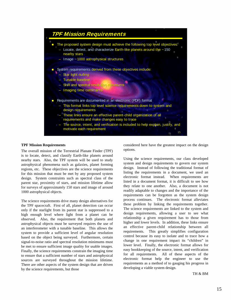
TPF Mission Requirements The overall mission of the Terrestrial Planate Finder (TPF) is to locate, detect, and classify Earth-like planets around nearby stars. Also, the TPF system will be used to study astrophysical phenomena such as galaxies, planet forming regions, etc. These objectives are the science requirements for this mission that must be met by any proposed system design. System constraints such as spectral class of the parent star, proximity of stars, and mission lifetime allow for surveys of approximately 150 stars and image of around 1000 astrophysical objects.

The science requirements drive many design alternatives for the TPF spacecraft. First of all, planet detection can occur only if the starlight from its parent star is suppressed to a high enough level where light from a planet can be observed. Also, the requirement that both planets and astrophysical objects must be surveyed requires the use of an interferometer with a tunable baseline. This allows the system to provide a sufficient level of angular resolution based on the object being surveyed. Furthermore, certain signal-to-noise ratio and spectral resolution minimums must be met to ensure sufficient image quality for usable images. Finally, the science requirements constrain the imaging time to ensure that a sufficient number of stars and astrophysical sources are surveyed throughout the mission lifetime. There are other aspects of the system design that are driven by the science requirements, but those

15

considered here have the greatest impact on the design options.

Using the science requirements, our class developed system and design requirements to govern our system design. Instead of following the traditional format of listing the requirements in a document, we used an electronic format instead. When requirements are listed in a document format, it is difficult to see how they relate to one another. Also, a document is not readily adaptable to changes and the importance of the requirements can be forgotten as the system design process continues. The electronic format alleviates these problem by linking the requirements together. The science requirements are linked to the system and design requirements, allowing a user to see what relationship a given requirement has to those from higher and lower levels. In addition, these links ensure an effective parent-child relationship between all requirements. This greatly simplifies configuration control because its easy to isolate and to trace how a change in one requirement impact its “children” in lower level. Finally, the electronic format allows for easy bookkeeping of the source, intent, and verification for all requirements. All of these aspects of the electronic format help the engineer to use the requirements as a method of to gauging his progress in developing a viable system design.

TH & BM

15

Software Requirements (TMAS)Software Requirements (TMAS)

A second set of requirements relates to the software that embodies the quantitative methodology

• Capture the essential physics that differentiatebetween competing architectures

• Establish and compare architectures based on a finite set of unified metrics including lifecycle cost

• Working seamlessly in one computing environment

• Can be easily extended to include additional capabilities and more detailed modeling (e.g. ODL’s)

• User-friendly a nd robust for all choices of a top level design vector

16

This charts summarizes the key requirements for the TPF mission analysis

software. It is important to recognize that the class was not only to meet

requirements for the TPF mission itself, but that there was a second set of

completely different requirements. This second set was a driver for the

design of the TMAS software itself and for the software development effort.

16

17

Flexible Team OrganizationFlexible Team Organization

Conceptual Design Phase

Preliminary Design Phase

Critical Design Phase

CDR Team Integration Team

Report Team

16.89 Class Participants

Dynamics, Optics ,Structures

Environment S/C Bus-Payload

GINA

Operations

Aperture

Coordination

This chart is supposed to illustrate the evolution of our team structure over

the course of the project. During the conceptual design phase the team had

frequent plenary meetings to discuss requirements and processes. This

required everyone’s participation. The preliminary design phase on the other

hand was characterized by individual work and bilateral coordination of

software, interface and other technical issues. Finally during the critical

design phase the organization had to change again to meet the new

requirements. The three teams CDR team, Integration team and the Report

team were created in order to ensure that the deliverables (1. CDR

Presentation, 2. TMAS Software and 3. Final Report) would become

available on time and within the expected quality. A conclusion from our

point of view is that a project organization cannot be rigid but must

continuously change during a project to meet the challenges of each phase

in view of the next milestone.

17

18

Attributes that Distinguish ArchitecturesAttributes that Distinguish ArchitecturesTop Trades Capability Metrics

Heliocentric Orbital Altitude (1 to 6 AU)

Aperture Maintenance (SCI vs. SSI)

Number of Apertures (4 to 12)

Size of Apertures (1 to 4 m)

Isolation (Angular Res.)

N/A

SSI allow more freedom in

baseline tuning

Fine tuning of transmissivity

function N/A

Rate (Images/Life)

Noise reductions increase rates.

Different operation delays

SSI power and propulsion

requirements highly sensitive

Increased collecting area improves rate

Increased collecting area improves rate

Integrity (SNR)

Different local zodiacal

emission and solar thermal

flux

SCI: passive alignment but

complex flexible

dynamics

Tuning of transmissivity

for exo-zodiacal suppression

Smaller FOV collects less

local zodiacal noise

Availability (Variability)

N/A

Different safing complexity and

operational events

Different calibration and

capture complexity

N/A

Aperture Environment S/CDyn & ControlsOperationsGINA

This chart is a cornerstone of the presentation since it establishes the relationship between the trade space for TPF and the metrics by which we will judge competing architectures. Thus it contains the attributes that distinguish individual architectures. There are fundamental relationships between the elements of the design vector and the capability metrics. For example the number of apertures in the system will directly affect our ability to shape the transmissivity function. This dictates the sharpness in the rise of the transmissivity at the boundary between the exo-zodi and the habitable zone. Hence the number of apertures drives the isolation metric (angular resolution).

The different attributes can be lumped into groups of modeling needs that will allow us to recognize important differences between competing architectures. These groups directly determined the macro-modules that would be require to capture the TPF-relevant relationships of physics, cost and systems engineering trades. Thus the level of modeling detail is high only for aspects that matter to TPF and that help us distinguish trends within the trade space. As mentioned before the shape of the transmissivity function, dynamic stability and thermal control are very important for the success of TPF. The communication system on the other hand was only modeled to the level of detail necessary to obtain a complete mission design. For example a link budget is included but not detailed analysis of time vs. frequency division multiplexing etc.. Such aspects might however become the key drivers for a trade analysis of a satellite communications constellation.

Chart: D.W.M , Text: dWo

18

19

Software Development ProcessSoftware Development Process

Define S/W Objectives &

Requirements

Define S/W Macro-Modules

Integrate Modules

Define All Interfaces

Code Modules

Define S/W Sub-Modules

Test Code

Benchmark Sanity Check

Ready For Use

Iterate to Improve Fidelity

Software Development Process The development of the TPF Mission Analysis Software (TMAS) entailed eight discreet steps, some of which were

executed in parallel: 1) Define S/W Objectives and Requirements 2) Define S/W Macro-Modules 3) Define All Interfaces 4) Define S/W Sub-Modules 5) Code Modules 6) Test Code 7) Integrate Code 8) Benchmark Sanity Check The first step entails defining exactly what user would like the software to do. For this class, the objective was to

create a software tool to enable comparisons of different TPF designs on order to map out the system trade-space. The required software inputs are the elements of the design vector (orbit, number of apertures, architecture, and aperture diameter), and the desired outputs are the GINA metrics. After defining the S/W objectives and requirements, the S/W macro-modules must be defined. Macro-modules represent distinct aspects of the design which have high coupling within each other, but low coupling between each other, allowing each macro-module to be coded individually by an individual/team with expertise in that area. TMAS contains six macr-modules: Environment, Aperture Configuration, Spacecraft (payload+bus), Structures/Control/Dynamics, Operations, and GINA. Once these macro-modules are defined, the interfaces (variable inputs/outputs) between them must be explicitly agreed upon by all of the programmers. This ensures compatibility between modules and speeds up the integration process. Interface definition is carried out in parallel with the selection of the macro and sub-modules, and is documented in the N2 diagram. The sub-modules are a division of each macro-module into it’s core components. For example, each spacecraft subsystem is a sub-module in the spacecraft macro-module. At this point, the code may be written. It is important that all of the code be thoroughly documented at this stage so that it may later be understood and modified with ease. As the modules are completed, they become integrated into a single “Master” code. In parallel with both the coding and integration, every module is continuously tested, both for correctness and compatibility. Finally, after all of the code has been integrated, simulations were run for existing TPF designs. By comparing the TMAS results with the documented design data, modeling errors are identified and the fidelity of the entire simulation is improved through an iterative process. Once the user is comfortable with the fidelity of the software, simulations may be run to map out the system trade-space.

19

20

Interface ControlInterface Control -- NN22 DiagramDiagram

�� Explicitly defines all inputs and outputs for macro and subExplicitly defines all inputs and outputs for macro and sub--modules.modules.

�� Notice the high coupling within macroNotice the high coupling within macro--modules and the lower couplingmodules and the lower coupling between modules.between modules.

�� Allows forAllows for ““plug and playplug and play””–– testingtesting–– alternative subalternative sub--modulesmodules

�� Provides a visual representation of the flow of information throProvides a visual representation of the flow of information through theugh thedesign process.design process.

�� FullFull--Sized NSized N22 Diagram provided separatelyDiagram provided separately

m-file

Inputs

Inputs

OutputsOutputs

Interface Control - N2 Diagram The TPF design process was divided into six macro-modules:

•Environment •Aperture Configuration •Spacecraft (Bus + Payload) •Dynamics, Optics, Control, & Stability (DOCS) •Deployment & Operations •Systems Analysis - GINA

Certain macro-modules were further subdivided into sub-modules. This modular division of the TPF design process reduces software development risk by reducing coupling and simplifies the simulation code development as each module is separately testable.

An N2 diagram is an N x N matrix used by systems engineers to develop and organize interface information (Boppe, 1998). The sub-modules (Matlab m-file functions) are located along the diagonal of the matrix. The inputs to each sub-module are vertical and the outputs are horizontal. The aggregation of the sub-modules into macro-modules is illustrated by the black boxes enveloping different sections of the diagonal.

The N2 diagram provides a visual representation of the flow of information through the conceptual design process and was used to connect all of the Matlab functions to enable an automated simulation of different TPF architectures.

20

3. TPF Mission Analysis Software (TMAS)3. TPF Mission Analysis Software (TMAS)

““This is one of the two main products of this effortThis is one of the two main products of this effort””

Summary:

The goal of this section is to lay out the structure and functional flow of the

macro-modules that make up TMAS. Simulink is used to show the

interdependencies of the individual modules and the flow of information.

The software has been implemented in MATLAB and the information is

passed back and forth in the form of data structures. The CDR will focus

more on the top-level issues and interconnections rather than on the

individual inputs, outputs and contents of the sub-modules, since this was

already done at the PDR.

21

22

Top Level Inputs and OutputsTop Level Inputs and Outputs

OrbitsOrbits

Interferometer TypeInterferometer Type

Size of ApertureSize of Aperture

Number of AperturesNumber of Apertures

TPF Mission Analysis Software

Inputs (Design Vector)Inputs (Design Vector)

Key OutputsKey Outputs

Total CostTotal Cost Total MassTotal Mass

Number of ImagesNumber of ImagesCost per ImageCost per Image

Top Level Inputs and Outputs

This slide shows the inputs and outputs of the TMAS, the TPF Mission Analysis Software. The inputs of the TMAS are the four design vectors including orbit from the Sun, number of Aperture, size of aperture, and interferometer type. The range of the inputs are shown in the following; Inputs Orbit: (1, 1.5, 2, 2.5, 3, 3.5, 4, 4.5, 5, 5.5, 6)AU Number of Apertures: (4, 6, 8, 10, 12) Size of Apertures: (0.5, 1.0, 1.5, 2.0, 2.5, 3.0, 3.5, 4.0)meter Interferometer Type: (SCI-Symmetric-1D, SSI-Symmetric-1D,

SCI-Symmetric-2D, SSI-Symmetric-2D)

The outputs of TMAS are the total cost, total mass, number of images, and cost per image. The units of each output are shown in the following;Outputs

Total Cost: (Millions $)Total mass: (kg)Number of images: (total number)Cost per image: (Thousands $/image)

22

23

TMAS Block DiagramTMAS Block Diagram

Design VectorDesign Vector

Orbit Number of Apertures

Size of Apertures Interferometer Type

Operations

Systems GINA

Spacecraft Bus/Payload

Aperture ConfigurationEnvironment

Dynamics, Optics, Control, & Structures

Total Cost Total # of Images

Cost/Image

MetricsMetrics

TMAS Block Diagram In order to determine the performance of a particular TPF design, a model for the design must be developed. This model must accurately depict the operation and performance of the system and must also be adaptable to different system configurations. We have divided this model into 6 macro-modules that focus on key parameters of the system design. The model, also known as the TPF Mission Analysis Software (TMAS), is designed to explore the multiple design options available for TPF and determine which configuration will maximize the system performance. The six macro-modules for TMAS were defined based on the most significant aspects of the system design. The model uses a design vector that is modified to help explore the trade space available to the system design. The TMAS block diagram shows how the information is flowed from the design vector through each of the macro-modules in order to obtain the performance metrics at the end of an iteration. Although each macro-module does not necessarily require information from the previous module, the linear organization makes it easy to basic function of the model. In reality, the TMAS program is actually much more complex than the block diagram would indicate. Most of the macro-modules include sub-modules that are used to model more detailed aspects of the system design. A Simulink model of

the TMAS program has been constructed to help to illustrate exactly how the software works.

The function of each macro-module is as follows: Environmental Provides interferometer’s local environment based upon the TPF operation orbit. Aperture Configuration Determines the optimal aperture configuration required to meet the science objective Spacecraft Bus/Payload Calculates the distribution of mass and power for the payload instruments and bus subsystems on each spacecraft in the TPF architecture Dynamics, Optics, Control & Structures Constructs a model of a given configuration to evaluate the interferometer’s achievable control and disturbance rejection performance. Operations Determines the required launch vehicle as well as the cost and risk associated with operation of the TPF system. Systems/GINA Computes the performance metrics for the architecture based upon inputs such as SNR, costs, mass, operations, etc.

TH & EK

23

24

Key EquationsKey Equations

Disturbance Effect

ωωωδωπ

σ dGG H zwwzwz )()()(1

0

2 ∫ ∞

=

Environmental and internal disturbances

Signal to Noise Ratio

Isolation and Integrity measures

Transmissivity function:

Nominal performance

( )[ ] ( ) 2

1 exp)cos(2exp∑

=

−= n

k kkkk jLjT D φφδλθπ

nn -- number of aperturesnumber of aperturesDDkk -- aperture sizeaperture sizeLLkk -- aperture lengthaperture lengthδδkk -- phasing anglephasing angleθθ -- point source angular separation from starpoint source angular separation from starλλ -- wavelengthwavelengthφφ -- point source separation from interferometerpoint source separation from interferometerφφkk -- independent phase shift for each apertureindependent phase shift for each aperture

The main goal of the engineering design is to reduce the effect of all disturbances in order to approach the nominal SNR

σσzz: RMS phase error: RMS phase errorδδww: Disturbance cross spectral density: Disturbance cross spectral density GGzwzw: Transfer function from disturbance to: Transfer function from disturbance to

performance outputperformance output

Key Equations In this and the following slides we state the equations that mainly capture the conceptual issues in the design of the TPF. The first aspect to be taken into account is given by the science requirements that drive the mission design. In this respect, the main performance measure is given by the quality of the nulling of the parent star by the interferometer. In the nominal case, this measure is given by the transmssivity function, that gives the percentage of the incoming light output at anomaly θ and wavelength λ. The transmissivity is a function of the geometric configuration of the array through the aperture sizes, baseline lengths, and phase delays. However, due to external and internal disturbances, the geometric configuration of the array will not always be at the nominal condition, hence some disturbance rejection devices have to be included in the system. The objective of the disturbance rejection can be formulated as a RMS optimization problem, that is the design objective is to minimize the resulting RMS on some parameters characterizing the geometric configuration, caused by the modeled disturbances. The overall effect of this design will be a performance measure that can be identified in a signal-to-noise ratio, that directly affects the Isolation and Integrity measures in GINA.

EF

24

25

Key equationsKey equations

Mission inefficiency

∑ =

+= n

i iitotaly rFDFCI

1

Cost per Image

Expected Utility

∫ ∑= =

T n

i ii dttPCTE

0 1 )()(

Launch cost look-up tables

Bus cost CERs

Payload cost

∝∝ ∑ =

N

i imirrors DC

1

67.2

Complexity due to events

( )( )ii

n

i i e Anf

mtte J −+=∑

=

1)(11 1

Total Cost

Number of Images

Cost per function measure

E= expected utility (#images) T= Total Mission Life i= specific system state T= total number of possible functioning states C= capability (imaging rate) in each state i P= probability of being in state i at time t

mttei: mean time to event i N: number of spacecraft

fi(N): relative event rate increment as a function of N

Ai: Automation level

Cy: average # of transmission cycles for anomaly resolution D: Transmission delay time Ftotal: Failure rate Fi: failure rate of specific ops function ri: average recovery time for specific ops function

Di: Diameter of aperture i N: number of apertures

Key Equations The optimization problem described in the previous slides cannot be solved independently from other consideration, among which perhaps the most important is the resulting cost of the overall system, as well as the cost per function allowed by the system. The total cost of the system can be split into the cost due to the launch vehicle, the spacecraft bus, the payload, and operations. Data about these cost components are obatined as follows: •launch vehicle: data about launch vehicle cost are available from the literature •spacecraft bus: Cost Estimate Relationships are used •payload cost: the payload cost is made of a fixed component (per collector/combiner) plus varaible part that increases with the size of the mirror. According to NGST estimates, the cost of mirrors are increasing as the diameter to the 2.67. •Operations cost: the evaluation of the operations cost is a very complex issue; however, cost is strongly related to the overall operations complexity, defined as:

n n n

J = Je +Jfe +Jf =∑ 1 1+ fi (n) 1−Ai + Xfe∑

1 1+ fi (n) +Xf ∑ 1 (1+ fi(n))

i=1 mttei i=1 mttfei i=1 mttfi ( )( ) ( )where mttei,mttfei,mttfi indicate the mean time to events, false events and permanent failures respectively, N is the total number

of spacecraft, fi(N) is a relative increase in the event rate as a function of N, Ai is the automation level, and finally Xfe and Xf are complexity adjustment factors,

Since the main function of the TPF system is to provide images of the target stars, we can define a cost per image to be used in the performance analysis. This cost per image is given by the total cost, divided by the total number of images that are expected to be taken over the whole mission duration. This number is given by:

256 n 313 n 365 n 1825 n Total Number Images = ∫ ∑CSiPi (t)dt + ∫ ∑CMiPi (t)dt + ∫ ∑CDiPi (t)dt +...+ ∫ ∑CDiPi (t)dt

74 i=1 257 i=1 314 i=1 1681i=1

where the limits of integration are the days for mode transition in the mission profile, i is the specific system state, n is the total number of possible functioning states, Csi, Cmi and Cdi are the capabilities (imaging rates) in each state i , respectively in Survey, Medium Spectroscopy, and Deep Spectroscopy mode, and finally Pi(t) is the probability of being in state i at time t. Moreover, a mission inefficiency parameter can be defined, that takes into account the efficiency loss due to the finite time required for anomaly resolution:

where Cy is the average number of transmission cycles for anomaly resolution, D is the transmission delay time, Ftotal is the total failure rate, and Fi and ri are respectively the failure rate and average recovery time for specific ops function.

n

I =CyDFtotal +∑Firi i=1

EF 25

26

Effect of RWA Noise on SNREffect of RWA Noise on SNR

Nor

mal

ized

Inte

nsity

Angular separation in sky

0.5 AU

Interferometer Transmissivity Function Reaction wheel imbalances cause

vibrations that “wash out” the transmissivity function

Example: ITHACO E-Wheel

Wheel speed 1000 +/- 1000 RPM Symmetric Pyramid of 4 Wheels

Nominal Test data : Scale factor =1.0 Increased Imbalances : Scale factor =10.0

SF=10 SF=1

“Washout” Effect

This chart shows the effect that the reaction wheel imbalances can have on the transmissivity function and ultimately the signal to noise ratio. The reaction wheel disturbance data was obtained from a test of the ITHACO E-Wheel conducted at NASA GSFC in 1998. The wheel speed distribution was assumed to be uniform between 0 and 2000 RPM. The combined effect of 4 wheels in a pyramidal configuration is taken into account.

The left subplot shows the effect of the reaction wheel imbalances that where obtained from the test without any modification to the test data. We see that the transmissivity has four symmetric lobes (fringes of peak intensity) and that the suppression of starlight meets the specification (upper left plot) of 10-6 out to the star diameter.

The right subplot however demonstrates the effect if the wheel imbalances are scaled up by a factor of 10. This could occur if the wheels are poorly balanced or if a ball bearing failure occurs during operations. The effect on the transmissivity is dramatic. Firstly we notice that a pair of fringes is now being washed out by the vibrations, secondly the nulling is no longer meeting requirements. In the nominal case the σOPD (average) is 76 nm, where it is 762 nm in the second case, which corresponds to roughly λ/16. For non-interferometric systems such a wavefront error might be acceptable. In the case of TPF it clearly is not and this is where the requirement for λ/6000 comes from. Thorough analysis and testing of reaction wheel imbalances before launch is paramount.

26

0.5 AU

27

Effect of Optical Control on SNREffect of Optical Control on SNR

10

10

Optical Control System improves nulling performance

Trade study shows that

optical control bandwidth

is insufficient at 5 Hz but

can meet the requirements

at 100 Hz

10 -4

10 -3

10 -2

10 -1

10 -12

10 -10

10 -8

10 -6

10 -4

10 -2

10 0

Nor

mal

ized

Inte

nsity

Angular separation in sky (arcsec)

Exo-solar system at 10 pc

Interferometer Transmittivity Function

5 Hz Optical Control BW 100 Hz Optical Control BW

σOPD=27.3 nm

σOPD=107 nm

Note: RMS OPD values shown are average for

all apertures

Requirement

4 Apertures, SCI, linear symmetric @ 1AU

This chart shows the level to which the dynamics and controls were captured. The effect of optical control on the system is modeled using a high-pass filter approach, where each OPD channel is attenuated by the optical control at low frequencies but not at high frequencies due to the limited sensor and actuator bandwidths .

The chart shows the effect of changing the optical control bandwidth on the transmissivity function. If the optical control bandwidth is too low, the optical pathlength differences between the apertures creates a time-varying phase difference φi between the light beams at the combiner. This phase shift disturbs the +/- 180 degree phase shift required for perfect nulling. A simplifying assumption is that the OPD’s which are the square roots of the variance of a stochastic random signal are added to the phase shift used to compute the transmissivity (see chart on key equations), as if they were deterministic. Thus the perturbations from the perfect transmissivity shown above are to be understand in a 1 sigma sense.

The preliminary results indicate that the science requirements cannot be met with an optical bandwidth of 5 Hz, but increasing the bandwidth to 100 Hz leads to sufficient suppression of the dynamic onboard disturbance sources.

27

28

Operations DefinitionsOperations Definitions

�� Operational Issues affect:Operational Issues affect:–– Development CostsDevelopment Costs–– Operations CostsOperations Costs–– System PerformanceSystem Performance

�� Development Costs:Development Costs:–– Flight SoftwareFlight Software–– Ground SoftwareGround Software–– FacilitiesFacilities–– EquipmentEquipment–– LogisticsLogistics–– ManagementManagement–– Systems EngineeringSystems Engineering–– Product AssuranceProduct Assurance –– Integration & TestIntegration & Test

�� Operations Costs:Operations Costs:–– MaintenanceMaintenance–– LaborLabor

�� System Performance:System Performance:–– Mission InefficiencyMission Inefficiency

Figure from ESA Cluster Mission

Operations Definitions Our TPF class, realizing that operations costs typically comprise a large percentage of total mission cost, decided to incorporate operational considerations into the design trade space. Usually operations design follows initial trade decisions made without operational input, but large differences in total mission cost and performance dependent on the operability of certain architectures encouraged an integrated approach. Areas of Impact Operational issues affect two main mission criterion: Cost and Performance. The cost can be further split into development cost and operations cost.Development costs are affected by the complexity level of the mission. More complex missions require longer flight and ground software codes, which have a snowball effect on other key development costs shown in the slide.

Operations costs consist of labor and maintenance costs, and affect the mission throughout its useful life. Labor costs are a function of crew size and salary which the class’s TPF software captures determines from estimated everyday operational complexity and failure recovery complexity. Maintenance costs are modeled on the size and complexity of the flight operations center.

System performance is affected by mission inefficiency, which is the science-gathering time lost from transmission delay time and anomaly resolution time.

-ARG

28

Effect of Operational Issues on SystemEffect of Operational Issues on System

Relative Operational Difficulty Increases with System Complexity Relatively Simple Relatively Complex

Structurally Few Many Connected Separated Separated Spacecraft Spacecraft Spacecraft

Mission Inefficiency grows with System Unreliability & Distance Relatively Small Relatively Large

Reliable system Less reliable system

(React Quickly to few anomalies) (React Slowly to more anomalies)

Close to Earth Far from Earth 29

Effect of Operational Issues on System This slide explains the two ways operational issues affect the total mission.

Operational difficulty leads to increased cost and is driven by system complexity. System complexity is driven, to a large degree, by the number of additional spacecraft to control, and the attendant increase in difficulty to ensure their cooperative functionality. Therefore, a structurally connected spacecraft is easier to operate than a small cluster of separated spacecraft, which, in turn, is easier to operate than a more numerous cluster of separated spacecraft. It should be pointed out that operating the five spacecraft of a 4 aperture SSI is not four or five times as complex as a single spacecraft SCI, since each additional collector spacecraft is comparatively simple with respect to the main combiner spacecraft. Furthermore, learning curve effects, operational efficiencies, and automation attenuate the complexity increase from each additional spacecraft. Mission inefficiency impacts system performance (primarily imaging rate) and is affected by two factors, system unreliability and distance. A less complex system will generate less anomalies, requiring less time to resolve those anomalies. A closer system will suffer less transmission delay time. Therefore, a close and reliable system reacts quickly to relatively few anomalies, while a distant and unreliable system reacts slowly to frequent anomalies.

29

30

Benchmark: Ball SCI TPFBenchmark: Ball SCI TPF

0

500

1000

1500

2000

2500

3000

3500

4000 M

ass

(kg)

Ball Estimate Class Estimate

Stru

ctur

e

Pow

er

CD&

HCo

mm

Ther

mal

ADCS

Prop

ulsi

on

Adj.

Prop

Payl

oad

Prop

ella

nt

Adj.

Prop

elTo

tal B

us, D

ryAd

j Tot

Bus

Dry

Tot

S/C

Dry

Ad

j Tot

S/C

Dry

Tota

l S/C

Wet

Adj T

ot S

/C W

et

Mass vs. System

0

500

1000

1500

2000

Pow

er (W

)

Average Power

5 AU

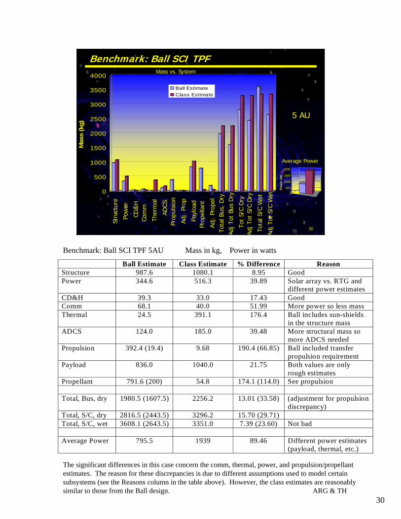
Benchmark: Ball SCI TPF 5AU Mass in kg, Power in watts

Ball Estimate Class Estimate % Difference Reason Structure 987.6 1080.1 8.95 Good Power 344.6 516.3 39.89 Solar array vs. RTG and

different power estimates CD&H 39.3 33.0 17.43 Good Comm 68.1 40.0 51.99 More power so less mass Thermal 24.5 391.1 176.4 Ball includes sun-shields

in the structure mass ADCS 124.0 185.0 39.48 More structural mass so

more ADCS needed Propulsion 392.4 (19.4) 9.68 190.4 (66.85) Ball included transfer

propulsion requirement Payload 836.0 1040.0 21.75 Both values are only

rough estimates Propellant

Total, Bus, dry

791.6 (200)

1980.5 (1607.5)

54.8

2256.2

174.1 (114.0)

13.01 (33.58)

See propulsion

(adjustment for propulsion discrepancy)

Total, S/C, dry 2816.5 (2443.5) 3296.2 15.70 (29.71) Total, S/C, wet

Average Power

3608.1 (2643.5)

795.5

3351.0

1939

7.39 (23.60)

89.46

Not bad

Different power estimates (payload, thermal, etc.)

The significant differences in this case concern the comm, thermal, power, and propulsion/propellant estimates. The reason for these discrepancies is due to different assumptions used to model certain subsystems (see the Reasons column in the table above). However, the class estimates are reasonably similar to those from the Ball design. ARG & TH

30

31

Benchmark TRW SCI TPFBenchmark TRW SCI TPF

0

500

1000

1500

2000

2500

3000

3500

4000

Mass (kg) S

truct

ure

Pow

er

CD

&H

Com

mun

icat

ions

Ther

mal

Prop

ulsi

on

Payl

oad

Prop

ella

nt

Tota

l, Bu

s

Tota

l, S/

C (d

ry)

Tota

l, S/

C (w

et)

TRW Estimate Class Estimate 5 AU

0 500

1000 1500 2000 2500 3000

Pow

er (W

)

Mass vs. System

Average Power

Benchmark: TRW SCI TPF 5AU Mass in kg, Power in watts TRW Estimate Class Estimate % Difference Reason

Structure 719.4 1207.1 67.8 TRW uses ultra lightweight truss with guy wire supports

Power 169.5 516.2 204.5 TRW uses lightweight solar concentrator

CD&H 41 69.0 68.3 Small total difference Communications 71.2 40 43.8 Small total difference Thermal 265 493 86 Propulsion 118.2 9.5 92 TRW included larger

propulsion rewuirement Payload 924.3 1118 21 Not bad Propellant

Total, Bus

250

753.3

53.5

1094

78.6

45.2

See propulsion

Total, S/C (dry) 2309.8 3602.5 56 Total, S/C (wet) 2559.8 3656 42.8 Average Power 2536.8 1939 23.6

The TRW design attempts to minimize mass using an ultra lightweight truss and lightweight solar concentrators. This, and the inclusion of a larger (possibly transfer) propulsion requirement accounts for a large share of the witnessed mass difference.

-ARG

31

32

Benchmark: TRW SSI TPFBenchmark: TRW SSI TPF

0

500

1000

1500

2000

2500

3000

3500

4000

4500

5000

Mass (kg)

Stru

ctur

e

Pow

er

CD

&H

Com

mun

icat

ions

Ther

mal

Prop

ulsi

on

Pay

load

Prop

ella

nt

Tota

l, Bu

s

Tota

l, S

/C (d

ry)

Tota

l, S

/C (w

et)

TRW Estimate Class Estimate

0 1000 2000 3000

4000

5000

6000

7000

Pow

er (W

)

Mass vs. System

Average Power

5 AU

Benchmark: TRW SSI TPF 5AU Mass in kg, Power in watts TRW Estimate Class Estimate % Difference Reason

Structure 289.7 885.4 205.6 Power 192.7 1135.3 489.5 Class needs more power,

therefore more mass. TRW uses lightweight solar concentrator

CD&H 33.2 69.0 107.8 Small total difference Communications 24.6 44.6 81.3 Small total difference Thermal 10.4 530.3 4999 TRW does not include its

sunshades Propulsion 55.4 306.4 453 Class has heavier buses Payload 676.2 1095 61.9 Propellant

Total, Bus

312.5

426.5

550.9

2544.4

76.2

496.6

Class has heavier buses

Total, S/C (dry) 2808.7 4250.1 51.3 Total, S/C (wet) 3121.2 4801 53.8 Average Power 346.2 6425 1755.9 Class figure includes sum

of all spacecraft using electric propulsion

TRW uses lightweight solar concentrators which are significantly less massive than the small nuclear power cells aboard each of the class’s electrically-propelled spacecraft. Also, TRW does not include the mass of the sunshades it uses into its calculations for SSI.

-ARG 32

4. Interactive Test Case4. Interactive Test Case

““A picture says more than a thousand wordsA picture says more than a thousand words””

Summary:

The goal of the interactive test case is to give the “customer” a first hand look

at the TMAS software and the sequence in which the analysis is run. A

number of figures are generated during the run that will be explained by the

most knowledgeable team member. A representative test case is chosen that

exercises most of the important sub-modules.

33

Input Design Vector with GUIInput Design Vector with GUI

The desired test cases are input

manually with the GUI; alternatively the TMAS software

can be run from a script in “batch” mode in order to

run a large number of cases without operator input.

34

In order to facilitate the running of the software a graphical user interface

was programmed for TMAS. The interface allows even the inexperienced

user to input a design vector and to execute the simulation automatically.

Another advantage of the GUI is that it only allows inputs to be made that

are within the allowable trade space. Thus a more detailed error checking

inside of the code can be avoided.

34

35

Interactive Test CaseInteractive Test Case

�� Design VectorDesign Vector–– Orbit:Orbit: 5.2 AU5.2 AU–– Number of Apertures:Number of Apertures: 44–– Architecture:Architecture: SCISCI--SymmetricSymmetric--2D2D–– Aperture Diameter:Aperture Diameter: [2 2 2 2] m[2 2 2 2] m

�� Pause statements have been inserted to enable us to see how eachPause statements have been inserted to enable us to see how eachpart of the TMAS code works.part of the TMAS code works.

-10 -8 -6 -4 -2 0 2 4 6 8 10 -6

-4

-2

0

2

4

6

Interactive Test Case The purpose of this interactive test case is to show the audience how TMAS

works firsthand in real-time. We will begin by entering the desired design vector into the graphical user interface (GUI). We will then proceed through an entire simulation run of TMAS, with several pauses during which we will explain how the program is working and what the results being displayed on the screen mean.

Some of the highlights of the interactive test case include: •Generation of the optimal aperture configuration •Design of the spacecraft bus to minimize total mass •Creation of a TPF finite element model •Mode animations •Control system design and performance •Operations Evaluation •GINA Systems Analysis

As each simulation requires several minutes to run, we will only be able to carry out one during the formal CDR presentation. After the CDR, however, please feel free to come up and try out your own design vector for TPF!

C.J.

35

5. TPF Mission Trade Studies5. TPF Mission Trade Studies

““Results and Conclusions from exploringResults and Conclusions from exploring the trade spacethe trade space ””

Summary:

This section demonstrates the results and conclusions that we obtained from

exploring the trade space with the TPF mission analysis software. We

demonstrate the dependence of a number of internal parameters such as

RWA imbalances and optical control bandwidth on the system performance.

More importantly the trades are made between the entries of the design

vector and our capability metrics. A useful metric for comparing very

different architectures is the cost per image metric, assuming that all images

(i.e. surveys) meet the required SNR requirements. Important trends have

become visible and first indications of “optimal” design corners are

becoming apparent.

36

37

Trade Study: Test MatrixTrade Study: Test Matrix

Orbits : 1Orbits : 1 -- 6 AU6 AU

Aperture Sizes :Aperture Sizes : 1m1m -- 4 m4 m

Number of Apertures : 4Number of Apertures : 4 -- 1212

Interferometer Type :Interferometer Type : One or Two DimensionsOne or Two Dimensions

Baseline Cases :Baseline Cases :OrbitOrbit -- 1 AU1 AUAperture SizeAperture Size -- 2 m2 mNumber of AperturesNumber of Apertures -- 44Interferometer Type:Interferometer Type:1D Linear Symmetric1D Linear SymmetricSeparatedSeparated

SpacecraftSpacecraftStructurallyStructurally

ConnectedConnected

Trade Study : Test Matrix The key objective of this project is to develop a framework in which the trade studies between different architectural design can be conducted. Taking a first step towards achieving this objective, the team has decided upon a test matrix where the results from the different cases can be compared when only one parameter in the Design Vector is varied at a time. In doing so, we would then be able to determine the trends by which certain parameters (cost, mass, etc.) change as a function of only one parameter. Even though we could have perform an exhaustive search for the “optimal” solution based upon the metric we chose to compare, understanding these single dimension trends gave us considerable insight as to what the sensitive parameters are and at the same time, confidence in our model. An exhaustive search of the trade space should only be performed once these key trades are understood. Based upon these results, it may be possible to reduce the search space from the possibly infinite number of designs.. In order to compare the different test cases, the team has chosen two architectures (SCI and SSI) as baseline cases where results from the other cases shall be compared to. The Design Vector parameters for the baseline case are: Orbit : 1 AU Aperture Size : 2 m Number of Apertures : 4 Interferometer : Linear Symmetric (SCI & SSI)

The Design Vector that the team has chosen consists of the (1) Orbit at which the interferometer is operating in, (2) the size of all the collector apertures, (3) the number of apertures and (4) the type of the interferometer (linear or 2­d arrays). The range in which these parameters are varied in this trade study are:Orbits : {1, 1.5, 2, 2.5, 3, 3.5, 4, 4.5, 5, 5.5, 6Aperture Size : {0.5, 1, 1.5, 2, 2.5, 3.0, 3.5, 4.0Number of Apertures : {4, 6, 8, 10, 12Interferometer Type : {Linear, Two Dimension}

EK & Class

37

..

i .

t

38

Trade Studies: OrbitTrade Studies: Orbit

Image Distribution vs. Orbit � At low orbits, the number of images is

limited by the higher noise level caused by the local zodiacal dust.

� For the same aperture configurations, this characteristic is independent of whether the spacecraft is SCI or SSI.

Cost Distribution vs. Orbit � As orbit increases, the most sizable

increases in cost are due to launch vehicle selection.

� The launch vehicle cost increases are primarily due to the increased Delta V requirements -- the total mass changes very little for the SCI case.

1 2 3 4 5 6 0

200

400

600

800

1000

1200

1400 SCI Image Distribution vs. Orbit

Orbit (AU)

Num

ber o

f Im

ages

Fine Spect Medium Spect Survey

1 2 3 4 5 6 0

200

400

600

800

1000

1200

1400 SCI Cost Distr bution vs Orbit

Orbit (AU)

Cost

(Mill

ions

$)

Payload Spac ecraft Bus Launch Vehicle Operations Developmen

Trade Studies: Orbit The orbital trade study was conducted on both an SCI and an SSI of the following configuration: 4 apertures; 2 meters diameter each; linear, symmetric arrangement.

Image Distribution vs. Orbit At low orbits, the number of images is limited by the lower SNR caused by the local zodiacal dust. In these orbits, the density of the dust relative to the light gathering power of the 2 meter collectors causes the integration time to be longer for each image. The plateau at about 1200 images represents the maximum number of images for this configuration based on factors other than orbit, such as instrument theoretical capabilities and other noise sources. For the same aperture configurations, the total number of images as a function of orbit is independent of whether the spacecraft is SCI or SSI.

Cost Distribution vs. Orbit As the orbital radius increases, the most sizable increases in cost are due to launch vehicle selection. Both the mass of the spacecraft and the Delta V requirements increase as the orbit increases, but it is the Delta V requirement that drives the cost increases in the SCI case. (See the next slide for more information on the mass trade.)

Development and payload costs do not show any dependence on orbit, while spacecraft bus and operations costs show the expected increases with higher orbits, primarily due to the longer mission lifetime.

38

tt

l . i

39

Trade Studies: OrbitTrade Studies: Orbit

Total Mass Distribution vs. Orbit � For this SSI case, the large mass increases

up to 4 AU are due to increasing solar array size to generate the required power.

� At 4.5 AU and higher, RTGs are selected by the TMAS.

� The growth in power system mass is driven further by the propulsion system, which must be more powerful (or use more propellant mass) to maneuver the greater total mass.

Total Mass vs. Orbit by Architecture � The multiple spacecraft in the SSI case

have a larger combined total bus mass than the SCI case.

1 2 3 4 5 6 0

1000

2000

3000

4000

5000

6000

7000 SSI Total Mass Distribution vs. Orbit

Orbit (AU)

Mas

s (kg

)

Propellan Struc ure Bus Payload

1 1.5 2 2.5 3 3.5 4 4.5 5 5.5 6 0

1000

2000

3000

4000

5000

6000

7000 Tota Mas s vs Orb t

Orbit (AU)

Mas

st (k

g)

Separated Spacecraft Structurally Connected

Trade Studies: Orbit Total Mass Distribution vs. Orbit As expected, the total mass of the spacecraft increases with orbital radius. The effect is much more pronounced for the SSI architecture. In this case, the propulsion systems on the separate spacecraft require a large amount of power relative to the rest of the spacecraft instruments to operate efficiently. Thus, as the orbit increases, the size of the solar arrays required to provide this power will grow until the TMAS determines that an RTG of an equivalent or smaller mass can provide the necessary power. For the orbit trade study architecture, this transition occurred at 4.5 AU. Propellant mass showed only a slight increase with orbit, indicating that rather than increasing propellant mass, it is more efficient to increase the power required by the propulsion system and to take the mass increase in the power system. The payload mass is not a function of orbit by the definition of this test case. The effect of orbit on bus mass is relatively small. In general, there is a slight positive correlation, but at the transition from solar arrays to RTGs, there is a more noticable jump due to the loss of the solar arrays as a layer in the passive cooling scheme. Total Mass vs. Orbit by Architecture The difference is due to the greater total bus mass associated with the multiple spacecraft in the SSI case. Not only do the multiple spacecraft require a greater initial mass, but the rate of increase with orbit is also greater due to the higher power requirements of the multiple propulsion systems. The dip in the graphs at 2.5 AU is due to a change in the thermal control scheme resulting from the lower solar heat flux.

39

40

Trade Studies: OrbitTrade Studies: Orbit

Cost per Image vs. Orbit � For low orbits, the higher cost per

image is largely due to the lower number of total images.

� For high orbits, the higher cost per image is largely due to higher launch costs.

� The higher cost per image of the SSI case is primarily due to the greater total mass (higher launch costs) and to higher initial development costs.

1 1.5 2 2.5 3 3.5 4 4.5 5 5.5 6

700

800

900

1000

1100

1200

1300 Cost per Image vs. Orbit

Orbit (AU)

Cost

per I

mag

e (T

hous

and

$/im

age)

Separated Spacecraft Structurally Connected

Trade Studies: Orbit Cost per Image vs. Orbit The total cost per image tends to increase at both ends of the orbital range, indicating that the optimum orbit (for the selected architecture) is within our range of consideration. However, one factor not included in the TMAS is an explicit evaluation of the potential effects of placing the TPF in the asteroid belt between 2.2 and 3.3 AU.

For low orbits, the higher cost per image is largely due to the lower number of total images. As discussed above, the lower number of images is due to the higher density of the local zodiacal dust that drives a longer integration time for each image.

For high orbits, the higher cost per image is largely due to higher launch costs. As mentioned previously, the higher launch costs are driven by the increased mass and Delta V requirements for the higher orbits.

The higher cost per image of the SSI relative to the SCI is primarily due to the greater total mass (higher launch costs) and to higher initial development costs. The development costs for the SSI case are higher due to the need to design (at least) two different spacecraft (collector and combiner) and to purchase more control system equipment rather than structural materials.

40

Trade Study : Number of Apertures (SCI)Trade Study : Number of Apertures (SCI)

Trade Study : Number of Apertures (SCI) In this trade study, only the number of aperture parameter in the Design Vector is varied and the results are compared to the baseline case. The trends for the expected number of images that can be obtained, the mass and the cost of the SCI architecture are shown. The results from these plots are discussed below: SCI Image Distribution The first plot shows the number of images that is expected increases with the number of apertures. The increase is most significant when the number of apertures is increased from four to six. Besides producing better transmissivity function (deeper and wider null) with higher number of apertures, this significant jump is seen mainly due to the assumptions made in the Markov model. In the Markov model, we assumed a total mission failure will occur when there are less than four operational apertures. Hence, in the four aperture case, the expected number of images that can be obtained is lower since this design cannot tolerate any failures. However, as higher number of apertures are used, we do not lose the entire mission when some of its apertures fail as long as there are at least four operational apertures.

�� Number of images increases with no. of apertuNum resber of images increases with no. of apertures–– Any failure in 4 aperture system causA esny failure in 4 aperture system causes

mission failuremission failure–– Better Transmissivity FunctioBett ner Transmissivity Function

�� Total mass increases linearly with no. of apertuTo restal mass increases linearly with no. of apertures–– DominateDominat d by dry massed by dry mass–– Little Propellant maLittle Propellant m ssass

�� Total cost increases linearly with no. of apertureTo stal cost increases linearly with no. of apertures–– Constant Development and Operation coCo stsnstant Development and Operation costs–– Differing launch vehicles (4, 6Differing launch vehicles (4, 6--10,10 121 apa ere turetu s)s, 2 p r re )–– Linear increase in Payload and Bus coLinea stsr increase in Payload and Bus costs

41

SCI Total Mass Distribution The plot of the interferometer’s mass as a function of the number of apertures shows the linear dependence of the total mass against the number of apertures. In all cases, the bulk of the interferometer’s total mass is dominated by its dry mass, of which more than 50% of it is the structural mass. On the other hand, the contribution of the propellant mass to the total mass is small. SCI Cost Distribution The total life cycle cost for this SCI designs increases with the number of apertures in the design. Both the development and the operation costs for this architecture remain constant since we are dealing with only one structure. As the number of apertures is increased, larger launch vehicles are required. In the case of 4 apertures, a Delta 3 rocket is required, while for the 6 - 10 aperture cases, a Delta 4 is required and the use of an Ariane 5 is required for the 12 aperture interferometer. Both the bus and the payload costs can be seen to increase linearly with the number of apertures, which is also a trend observe with the bus and payload masses.

E.K

41

Trade Study : Number of Apertures (SSI)Trade Study : Number of Apertures (SSI)

�� Number of images increases with no. of apertuNum resber of images increases with no. of apertures–– Any failure in 4 aperture system causA esny failure in 4 aperture system causes

mission failuremission failure–– Better Transmissivity FunctioBett ner Transmissivity Function

�� Total mass increases with no. of apertureTo stal mass increases with no. of apertures–– Dry mass increases lineaDry mass inc rlyreases linearly–– Significant propellant maSig ssnificant propellant mass

�� Total cost increases with no. of apertureTo stal cost increases with no. of apertures–– Linear increases in Development, OperatioLinear inc n, Bus &reases in Development, Operation, Bus &

Payload costPayload cos sts–– Differing launch vehicles (4Differing launch vehicles (4--6, 86, 8--10, 12 apert10, 12 ures)uapert res)

Trade Study : Number of Apertures (SSI) Similar to the results in the previous slide, the trends for the Separated Spacecraft Interferometer design as the number of apertures is varied are presented here. SCI Image Distribution Similar to the SCI results, the expected number of images increases with the number of apertures. Again, a sharp increase in the total number of images is again observed when the number of apertures is increased from four to six and again, this can be attributed to the assumptions made in the Markov model. Note that except for the four spacecraft case, the expected number of images is higher than the results shown in SCI design. This is mainly attributed to allowing the separated apertures to re­position to a different set of optimal imaging locations when one or more apertures fail. For example, the SSI apertures in an optimal six aperture configuration can be re-configured to assume the optimal five aperture configuration when one of them fail. This option, however, is not available to the SCI and will therefore, explain the lower number of images obtained.

42

SSI Total Mass Distribution Similar to the SCI design, the total mass of the interferometer is dominated by the dry mass of the interferometer. However, in this case, the propellant mass makes up quite a significant portion of the total spacecraft mass. In reality, the amount of propellant required for the SSI is in fact lower, since one can take advantage of square maneuvering profiles where the spacecraft can be allowed to drift while no propellant is expended. The propellant calculation in this trade study assumes the spacecraft traverses in a circular trajectory.

SSI Cost Distribution Except for the sudden jump in the launch vehicle cost, the life cycle cost for this design increases approximately linearly with the number of apertures. The services of a Titan 4 is required for the 12 aperture case, while the 8 and 10 aperture cases require an Ariane 5 class launch vehicle and the 4 and 6 aperture interferometers require a Delta 4 rocket.

E.K

42

i

t

ii

t t ll

43

Trade Study : Number of Apertures (SCITrade Study : Number of Apertures (SCI vsvs SSI)SSI)

�� SCI has better Cost per Function performanceSCI has better Cost per Function performance–– Best performance at 8 aperturesBest performance at 8 apertures

�� SCI has lower total massSCI has lower total mass–– Higher Structure mass in SCIHigher Structure mass in SCI–– Higher Bus & Propellant masses in SSIHigher Bus & Propellant masses in SSI

�� SCI has lower overall costSCI has lower overall cost–– Lower Development cost in SCILower Development cost in SCI–– Higher Operations & Bus costs in SSIHigher Operations & Bus costs in SSI

4 5 6 7 8 9 10 11 12 700

800

900

1000

1100

1200

1300 Cost per mage - SCI vs SSI

Number of Aper ures

Cos

t per

mag

e ($

1000

/ mag

e)

S ruc ura y Connected Separated Spacecraft

Best PerformanceBest Performance

Trade Study : Number of Apertures (SCI vs SSI) Comparison between the two architectures (SCI and SSI) as the number of apertures is varied is presented in the slide. Total Mass Distribution - SCI vs SSI Comparison between the two architectures over the range of apertures shows a higher total mass in the SSI case. This is mainly attributed to the added spacecraft buses, structure and propellant required for each aperture. In general, the SCI requires more structural mass but surprisingly, its overall dry mass is less than that required by the SSI. This lower dry mass in SCI could very well due to the rather short aperture separations required. In this analysis, we have considered planet detection as the key objective and only a maximum baseline of 120 m is required. However, if one were to take into consideration the second science requirement where milli-arcsec resolution imaging is required, aperture separations of at least 1 km are required. This will inherently increase the structural mass of the SCI architecture significantly. Correspondingly, the amount of propellant required to maneuver the different spacecraft in the SSI case will increase too. The impact of varying the aperture separations has on the overall architectural mass should be investigated

Cost Distribution - SCI vs SSI Consistent with the trend observe in the architectural mass comparison, the life cycle cost of the SSI is higher than the SCI. This is true especially for designs with high number of apertures. This higher SSI cost can be attributed to several factors: (1) more massive design (from mass comparison), (2) larger launch vehicles required, (3) more complex operation scenario and (4) higher development cost, since SCI is possibly more technologically mature compare to realizing a SSI design.

Cost per Image - SCI vs SSI Even though the SSI has higher life cycle cost, comparisons between the architectures should be perform based upon the design’s cost per function metric. In this case, the metric is the amount (in $1000) per useful image. This third plot shows the cost per image for the two architectures. Even though we observe rather significant difference in the architecture’s life cycle cost, the difference in cost per image metric is not as high. This is mainly due to the higher number of images that can be expected from the SSI design. In both cases, the “optimal” solution is to use the 8 aperture configuration.

E.K

43

i i i i

i i i i

l

l

44

Trade Studies (Interferometer TypeTrade Studies (Interferometer Type -- 1)1)

Image Distribution vs. Interferometer Type – The 1-dimensional, symmetric

architectures have superior imaging capability.

– The 2-dimensional architectures collect less images because of nulling losses. (counter-intuitive result)

– The 4 collector array does not demonstrate the graceful degradation advantage of the SSI architecture.

Mass Distribution vs. Interferometer Type

– There is almost no mass difference between the 1-dimensional and the 2-dimensional architectures.

– The SSI architectures are more massive because each spacecraft requires a separate bus and the propulsion system is relatively inefficient.

SCI, 1-D Symmetr c

SCI, 2-D Symmetr c

SSI, 1-D Symmetr c

Fine Spect.Medium Spect.Survey

0

100

200

300

400

500

600

700

800

900

1000 Image Distribution

Num

ber o

f Im

ages

Interferometer Type

SSI, 2-D Symmetr c

Total Mass Distribution

0

500

1000

1500

2000

2500

3000

3500

4000

4500

5000

Mas

s (k

g)

SCI, 1-D Symmetr c

SCI, 2-D Symmetr c

SSI, 1-D Symmetr c

Interferometer Type

SSI, 2-D Symmetr c

Propel ant Structure Bus Pay oad

Trade Study: Interferometer Type The architectures of interest for the systems level analysis of TPF are the: the SCI and SSI, 1 and 2 dimensional cases. (All architectures evaluated thus far, were symmetric designs.)

These four interferometer choices were traded for the (constant) configuration of 4 apertures, each having a 2 meter diameter; orbiting at 1 AU.

Image Distribution vs. Interferometer Type The number of images, appears to be more dependent on the aperture configuration than on architecture type. In this case, the one-dimensional architectures out perform the two-dimensional ones. This is a counter-intuitive result because we naturally expect the two dimensional to be more efficient. But the two-dimensional case does not null as well the one-dimensional case. (Please consult Edmund if a question arises.)

We would also expect the SSI case to be more efficient, a distinct architecture advantage. This trade, however, does not show the graceful degradation capability of the SSI configuration. The four aperture SSI (based on our failure analysis) is the smallest SSI configuration allowed. So a single collector failure will cause a system failure, much like it always occurs in the SCI architecture. If a 3 or 2 collector array was feasible, then the 1-D SSI architecture would gain an advantage. This advantage would also become clear if our baseline design consisted of more than four spacecraft.

Total Mass Distribution vs. Interferometer Type The total mass of the SSI architecture is clearly larger the total mass of the SCI architecture. There are several contributors to the additional SSI mass. Some examples include the fact that: each collector spacecraft requires its own bus, the propulsion system must operate over a large range of thrusts which is inherently inefficient, and the structural mass savings (initially thought to be considerable) is minimal.

-BM

44

i i i i

i

i i i i

i

l

45

Trade Studies (Interferometer TypeTrade Studies (Interferometer Type -- 2)2)

Cost Distribution vs. Interferometer Type – Cost appears to scale with mass

and complexity, favoring the SCI architectures

– There is no substantial cost difference between 1-dimensional and 2-dimensional architectures.

Cost per Image vs. Interferometer Type – The SCI 1-Dimensional architecture

has a high imaging rate and is reasonably cheap, so it produces the “best” combined performance.

– This “best” architecture will likely change as the design vector changes.

0

200

400

600

800

1000

1200

1400

1600

1800 Cost per Image

Cos

t per

imag

e ($

1000

/imag

e)

SCI, 1-D Symmetr c

SCI, 2-D Symmetr c

SSI, 1-D Symmetr c

Interferometer Type

SSI, 2-D Symmetr c

0

200

400

600

800

1000

1200 Cost Distribution

Cos

t ($M

llion

s)

SCI, 1-D Symmetr c

SCI, 2-D Symmetr c

SSI, 1-D Symmetr c

Interferometer Type

SSI, 2-D Symmetr c

Spacecraft Bus Launch Vehicle Operat ons Development

Pay oad

Trade Study: Interferometer Type … continued

Cost Distribution vs. Interferometer Type The cost distribution appears to scale with mass and complexity, so the SSI architecture is duly penalized. The largest increases in cost come with extra development cost (presumably due to complexity) and with extra bus cost (due to the increase in bus mass). The net difference in mass between the SCI and SSI architectures is small enough, though, that there is negligible launch vehicle penalty. As mass increases, we are sure to a see a launch vehicle effect on the interferometer trade.

Cost per Function vs. Interferometer Type The cost per function is a combined metric attempting to capture both the performance and the cost we pay for that performance. In this case, the one-dimensional SCI architecture has the “best” cost per function. This is quite obvious because the one-dimensional SCI case matches the performance of the one-dimensional SSI case for the cost of the two-dimensional SCI case. The “best” architecture will likely change as the design vector changes. It is difficult to project the changes of the cost per function, because it incorporates both image distribution and cost (mass and complexity) effects. Please review the former sections to estimate these changes.

-BM

45

i

i

i

t i

lft

l

46

1 1.5 2 2.5 3 3.5 4 0

500

1000

1500 Cost vs Aperture size

Aperture D ameter (m)

Cost

(Mill

ions

$)

Operations Launch Veh cle Spacecraft Bus Payload

1 1.5 2 2.5 3 3.5 4 0

500

1000

1500 Cost vs Aperture s ze

Aper ure D ameter (m)

Cos

t (M

illio

ns $

) Operations Launch Vehic e Spacecra Bus Pay oad

Trade Study: Aperture DiameterTrade Study: Aperture Diameter

•The payload cost increases as D2.67

•The operations/development cost is independent of aperture size, and is higher in the case of separated spacecraft, because of the increased system complexity; •The bus cost is higher for the separated spacecraft case, as it scales with the number of independent spacecraft; •Launch cost are approximately equal in the two cases.

•Cost breakdown

Trade Study: Aperture Diameter We want to analyze the effect in the system performance and cost due to variations in the aperture diameter, keeping all the other design variables fixed.As a first step, we analyze the effects on the overall cost, and on the cost components, due to the variation in aperture size.First of all, we notice, as expected, that the payload cost increases as the aperture size increases. The payload cost can be split into a fixed component and a component that varies with the mirror size. This variable component is proportional to the aperture diameter to the 2.67.The operations/development cost is largely independent of the aperture size, and it is indeed constantin the above plots. Moreover, we notice that this cost component is considerably bigger in the SSIcase, due to the increased complexity of the SSI system over the SCI.The bus costs are higher in the SSI case, since we have to duplicate components for each and every one of the independent spacecraft, and increase with the aperture size, since bigger mirrors requiremore capabilities from the bus (e.g. thermal system). The SSI and SCI bus costs can be seen to differ by a constant term.Finally, the launch costs are essentially the same for the two cases. However, we notice that for D=4m in the SSI case, we have a jump in the launch cost. This is due to the fact that the total systemmass exceeds the capabilities of the previously selected launcher, and requires a more expensive launch system.As a consequence of the above trends, the total costs in both the SSI and SCI cases grow more than quadratically with the aperture size. The cost difference, on the other hand, appears to be constant,and is due mainly to the cost difference in the operations/development, and secondarily to differentbus costs.

EF

46

i

..

i

t i

/i

-

47

Trade Study: Aperture DiameterTrade Study: Aperture Diameter

1 1.5 2 2.5 3 3.5 4 0

200

400

600

800

1000

1200

1400 Number of Images vs Aperture D ameter

Aperture Diameter (m)

Num

ber o

f Im

ages

Survey Medium Spect Fine Spect �� As aperture diameter increases,As aperture diameter increases,

the total energy collected per unitthe total energy collected per unit time increases, thus resulting in atime increases, thus resulting in a shorter integration timeshorter integration time forfor imaging purposes.imaging purposes.

�� The effect is the same for SCIThe effect is the same for SCI and SSI architectureand SSI architecture

1 1.5 2 2.5 3 3.5 4 0

500

1000

1500

2000

2500

3000 Cost per mage

Cos

per

mag

e ($

mag

e)

Aperture Diameter (m)

SCI SSI SSI SCI

�� TheThe cost per imagecost per image shows ashows a minimum at the right end of theminimum at the right end of the range that has been considered,range that has been considered, atat 3.5m3.5m in the SSI case, and atin the SSI case, and at 4m4m in the SCI casein the SCI case

�� TheThe costcost difference between thedifference between the architectures remains approx.architectures remains approx. constant across most of the rangeconstant across most of the range (ops+bus cost difference)(ops+bus cost difference)

The increased collection area allows for a bigger harvest of photons from the target; as a consequence, the integration times required for each image will be reduced accordingly. Since we are considering a constant time delay between observation, it can be easily seen that as the aperture diameter grows, the total number of images per unit time goes to some asymptotic value. This effect is the same for both SSI and SCI cases. The cost per image shows a generally decreasing behavior in the range we have considered, showing optimum values at the right end of the plot. The SSI case presents a very slight minimum at 3.5m, due to the increase in the launch cost for d=4m discussed in the previuos slide. Since the total cost increases as D^2.67, while the total number of images approaches a constant value, the cost per image will eventually increase at the same rate as the total cost. This means that the cost per image will have some minimum value, that form the plot above appears to be close to 4m. On the other hand, the cost difference approaches a constant value, as it will eventually be the ratio of two constants.

On the very limited trade space analyzed here, it appears that an SCI architecture with D=4m would be the optimum with respect to the aperture size.

EF

47

Summary of Trade StudiesSummary of Trade Studies

�� OrbitOrbit

–– Total Number of Images, Mass, and Cost increase as Orbit increasTotal Number of Images, Mass, and Cost increase as Orbit increases.es.–– Same Number of Images for SSI and SCSame Nu I.mber of Images for SSI and SCI.–– Higher Total Mass, Cost, and Cost per Image for SSI than SCHigher To I.tal Mass, Cost, and Cost per Image for SSI than SCI.–– Lowest Cost per Image is when Orbit is at 2.5 AU for SCLowe I.st Cost per Image is when Orbit is at 2.5 AU for SCI.

�� Number of ApertureNumber of sApertures

–– Total Number of Images, Mass, and Cost increase as Number of ApeTotal Number of Images, Mass, and Cost increase as Number of Aperturesrtures increases.increases.

–– More Images for SSI than SCI except when Number of Aperture is 4More Images for SSI than SCI except when Number of Aperture is 4..–– Higher Total Mass, Cost, and Cost per Image for SSI than SCHigher To I.tal Mass, Cost, and Cost per Image for SSI than SCI. –– Lowest Cost per Image is when Number of Aperture isLowe 8 for SCI.st Cost per Image is when Number of Aperture is 8 for SCI.

48

Summary of Trade Studies (Orbit, Number of Apertures)

This slide summarizes the key relationships discovered from the trade studies of orbit and number of apertures.

Orbit: Generally, the total number of images, mass, and cost increase as orbit

increases. The number of images reaches the maximum of about 1200 images after about 3 AU because the effect of the local zodiacal dust becomes small. Therefore, orbit does not influence the number of images any more. The same number of images are expected for both SSI and SCI with the same number of aperture and size of aperture. SSI in general will have higher mass and cost. Since the total number of images is the same for both SSI and SCI, the ratio of total cost over the number images, cost per image, is lower for SCI. The lowest cost per image is when orbit is 2.5 AU for SCI. Unfortunately, 2.5 AU is located in the asteroid belt, so future work is required to see if this orbit is feasible for TPF.

Number of Aperture: Total number of images, mass, and cost increase as the number of apertures

increases. SSI produces more images than SCI except when number of aperture is 4. This trade study shows that the total mass, cost, and cost per image is higher for SSI than SCI. The lowest cost per image for both SCI and SSI happens when number of aperture is 8.

SP

48

Summary of Trade StudiesSummary of Trade Studies

�� Size of ApertuSize of Apert reure

–– Total number of images, total cost increases as aperture diameteTotal number of images, total cost increases as aperture diameterr increasesincreases

–– Same number of images for SSI and SCSame n Iumber of images for SSI and SCI–– Lowest cost per images is when aperture diameter is 3.5 m for SSLowest cost per images is when aperture diameter is 3.5 m for SSI andI and

4 m for SC4 m for S I.CI.

�� InterferometerInterfero Typemeter Type

–– Higher mass and cost for SSIHigher ma .ss and cost for SSI.–– 1D has higher imaging rate than 2D.1D has higher imaging rate than 2D.–– SCI 1D has the Lowest CostSCI 1D ha per Image.s the Lowest Cost per Image.

49

Summary of Trade Studies (Size of Aperture, Interferometer Type)

This slide summarizes the key relationships discovered from the trade studies of size of aperture and interferometer type.

Size of Aperture: As the aperture diameter increases, the total number of images, and total cost

increase. Total cost increases as diameter^2.67 and total number of images increases until it meets its asymptotic value. The total number of images for both SSI and SCI are the same for the same aperture diameter. The lowest cost per image is when the aperture diameter is 3.5 m for SSI and 4 m for SCI. Since the total number of image reaches constant after 4 m and the cost increases as the size of aperture increases, the ratio of these two, the cost per image, will start to increase after 4 m.

Interferometer Type: The trade study of Interferometer type vs. outputs shows that cost and mass

of SSI are generally higher than SCI. 1D has higher imaging rate than 2D for both SSI and SCI. Combining these two trends produces a result that SCI 1D generates the lowest cost per image.

SP

49

i

i

-

-

-

50

Operational Trade ResultsOperational Trade Results

0 1 2 3 4 5 6 70

5

10

15

20

25

30

35

40 Mission Inefficiency vs. Orbit

Orb t (AU)

Mis

sion

Inef

fic e

ncy

(min

utes

/day

) SCI

SSI 4 ap

SSI 8 ap

0

5

10

15

20

25

30

35 Operations Cost Breakdown

Cos

ts ($

M)

YEARLY MAINTENANCE

AVG. YEARLY LABOR

SCI-4ap SSI-4ap SSI-8ap SSI-12ap

Crew SizesCrew Sizes–– Small transit staff, large checkout staff,Small transit staff, large checkout staff,

steadysteady--state science staffstate science staffOperations CostsOperations Costs–– Jump in maintenance cost from SCI to SSI.Jump in maintenance cost from SCI to SSI.–– Labor cost grows with number of spacecraftLabor cost grows with number of spacecraft

Mission InefficiencyMission Inefficiency–– Increases with distance, but faster for moreIncreases with distance, but faster for more

complex spacecraftcomplex spacecraftTime in years

0 1 2 3 4 5 6 7 0

50

100

150

200

250

300

350 Crew Sizes vs. Time (1AU cases)

Cre

w S

ize

SCI-4ap

SSI 4ap

SSI 8ap

SSI 12ap

Science Phase Checkout Phase

Tran

sit P

hase

Operational Trade Results The previous trades presented in the preceding few slides varied one of the four parameters in the design vector to determine the effect of that parameter on the total system. Eventually, we wish to fill in our entire trade space by varying several parameters to arrive at an optimal solution for a chosen system metric. The operations trade study captures the dynamics of the operational component while several variables are changed. Since operations cost and operationally-derived performance losses have such a large impact on total mission cost and performance, it behooves the mission designer to understand the coupling of operations with the other design vectors. Crew Sizes vs. Time Different staffing levels will be required at different times during the mission. The graph in the upper right corner shows the effect of time on the crew levels of four different configurations. The increase in complexity between the SCI and more complex SSI types increases the crew levels, despite learning curve effects of operating more similar spacecraft. Increasing the distance at which the TPF operates (e.g from 1 to 5 AU) would tend to increase the transit time and cost.

Ops Cost Breakdown

In the graph in the lower right corner we witness the effect of increasing mission complexity on two different components of operational cost. Notice the large jump in yearly maintenance between the SCI and the least complex SSI. This represents the difficulty from switching from a single satellite ops scenario to a constellation and the attendant increase in control center size and capability. Also notice that further increases in complexity to 8 and 12 aperture SSI configurations have only a marginal effect on yearly maintenance. Labor costs increase relatively linearly between the architectures shown. Steady-state maintenance and labor costs are relatively independent of final orbit.

Mission Inefficiency vs. Orbit

The graph in the lower left corner shows the increase in mission inefficiency with orbit for three system configurations. The SCI closest to earth has the least inefficiency while the most complex SSI farthest away has the most. Notice also that the rate of inefficiency increase is greatest for the SSI with 8 collector spacecraft.

-ARG11

50

51

6. Conclusions and Recommendations6. Conclusions and Recommendations

““ We have presented our resultsWe have presented our results ……What conclusions can we draw from them ?What conclusions can we draw from them ? ““

This section shows the cases that provided the best performance in terms of cost per

image. Also we are showing the results from two combined SCI and SSI cases.

Furthermore we are discussing future work as well as lessons learned from this

class.

51

Best Cost Per Image Performance (SSI)Best Cost Per Image Performance (SSI)

Best SSI Design from the 25 cases:Best SSI Design from the 25 cases:OrbitOrbit : 1 AU: 1 AUAperture SizeAperture Size : 2 m: 2 mNumber ofNumber of AperturesApertures : 8: 8InterferometerInterferometer : Linear Symmetric: Linear Symmetric

Total MassTotal Mass : 7758 kg: 7758 kgLaunch VehiclLaunch Ve ehicle : Ariane 5: Ariane 5Number of ImagesNumber of Images : 1332: 1332Total CostTotal Cost : $1.16: $1.1 Billion6 BillionCost Per ImageCost Per Image : $871,2: $87 6761,2 7

52

Best Cost Per Image Performance From the 25 different cases that we ran to determine the different trends, the best cost per image performance by a Separated Spacecraft Interferometer design is to operate a linearly symmetric interferometer using 8 apertures at 1 AU distance from the sun. This result is different to the Structurally Connected Interferometer where the best performance there occurs when operating orbit of the interferometer is varied from the baseline case. Note that the best design shown here is by no means the optimal design since we have only sampled a very small portion of the trade space. The key objective of this result indicates the capability of our methodology to determine the “best” solution using the assumptions we have made

52

Best Cost Per Image Performance (SCIBest Cost Per Image Performance (SC )I)

BestBest SCI DeSC signI Design from the 25 cases:from the 25 cases: OrbitOrbit : 2.5 AU: 2.5 AUAperture SizeAperture Size : 2 m: 2 mNumber ofNumber of AperturesApertures : 4: 4InterferometerInterferometer : Linear Symmetric: Linear Symmetric

Interesting comparisonTotal MassTotal Mass : 3372: 3372 with SSI case,Launch VehiclLaunch Ve ehicle : Delta 4: Delta 4 better $/image performanceNumber of ImagesNumber of Images : 1171: 1171

but smallerTotal CostTotal Cost : $789.9 Million: $789.9 MillionCost Per ImageCost Per Image : $674,0: $67 0004,0 0 less capable mission than SSI

53

Best Cost per Image Performance (SCI)

2.5 AU 4 Apertures SCI - Linear Symmetric 2m apertures

This chart presents the best case from the previous trade studies (25 cases) when only one parameter is varied at the same time. We see that the largest benefit seems to come form going out to 2.5 AU. This effect leads to a shorter integration time for a given SNR due to the reduced local zodiacal noise. This in turn leads to a larger number of images over the lifetime.

It is interesting to compare this architecture with the previous SSI case. We see that it provides significantly better cost/image performance . In general it is a very different mission than the SSI mission. The total system mass is about half of the SSI case and launch vehicle costs, system complexity (optics design, ADCS design) is much simpler. Even though the $/image performance is better the versatility of the instrument (especially if we were to include astrophysical imaging) is also lower than in the SSI case.

53

Combined Case (SCI)Combined Case (SCI)

Combined Case SCI :Combined Case SCI : This design obtained by OrbitOrbit : 2.5 AU: 2.5 AU taking the minima from theAperture SizAperture Si eze : 4 m: 4 m trade studiesNuNummbbeerr ofof AAppertuertureressIntInteerrfferomerometeteerr : Linear: Linear SymmetricSymmetric

: 8: 8

Total MassTotal Mass VehicleVehicle

: 756: 7567 kg7 kg:: Too LargeToo Large **

Number of ImagesNumber of Images : 2440: 2440Total CostTotal Cost : $1.26: $1.2 Billion6 BillionCost Per ImageCost Per Image :: $518,000$518,000

Is this the best case ?

Provides the lowest $/image of all cases we ran but it is WRONG to claim that this is the absolute best , since we have not fully explored the trade space

54

This case results from taking the local minima in the (one-dimensional) trade studies and using them to create a combined case for the SCI. We can see that the resulting cost/image is indeed the lowest for all of the cases we ran. It would however be WRONG to claim that this is the absolutely best architecture since we have not conducted an exhaustive search of the trade space.

Our recommendation for the future is to refine and validate the methodology, conduct sensitivity analysis and to search the ENTIRE trade space to find the globally best architecture.

54

55

Combined Case (SSI)Combined Case (SSI)

Even though SSI consistently has greater $/image it provides greater flexibility, which is not captured in the current model.

Combined Case SSI :Combined Case SSI :OrbitOrbit : 2.5 AU: 2.5 AUAperture SizeAperture Size : 3.5 m: 3.5 mNumber of AperturesNumber of Apertures : 8: 8InterferometerInterferometer : Linear Symmetric: Linear Symmetric

Total MassTotal Mass : 12998 kg: 12998 kgVehicleVehicle :: Too Large *Too Large *Number of ImagesNumber of Images : 2182: 2182Total CostTotal Cost : $1.58 Billion: $1.58 BillionCost Per ImageCost Per Image :: $727,000$727,000

This design obtained by taking the minima from the

trade studies for SSI

Is this the best SSI case ?

14%

23%

34%

19%

11%Lifecycle Cost

BusDevelopmenLauncOperations

Payload

Even though the mass is very large for this architecture, this could be split

into several launch vehicles since we are in the SSI case. Also here it is not

correct to claim that this is the best architecture since we have not

performed an exhaustive search of the trade space.

55

List of DeliverablesList of Deliverables

�� Annotated ViewgraphsAnnotated Viewgraphs–– TARR, PDR, CDRTARR, PDR, CDR

�� Requirements DocumentRequirements Document–– Electronic VersionElectronic Version

�� Architecture Analysis DocumentArchitecture Analysis Document–– Detailed Final ReportDetailed Final Report

�� Journal ArticleJournal Article–– Summary of Class EffortSummary of Class Effort

56

List of Deliverables

This slide shows the list of deliverables generated throughout all the design phases. During each presentation (TARR, PDR, and CDR), printed slides with annotation were generated. Initial of the contributors was added on each annotation.

Requirements Document was initially generated during the Conceptual Design Phase and went through continuous revision and updates during other design phases. The final version of the Requirements Document is in electronic version.

The Architecture Analysis Document is the detailed final report that will be turned in after the CDR. It includes project overview, the TPF mission description, architectural design approach, architectural design options, architectural design evaluation modules, architectural design evaluation results, and conclusion. It also include the copy of TMAS as an appendix. The Report Team, consists of André Girerd, Emilio Frazzoli, and Andrew Curtis, is leading in collecting sections from each member and integrating them to a final report.

Finally, a journal article will be written to summarize the class effort and published in a journal.

56

Future WorkFuture Work

�� Integration & AnalysiIntegratio sn & Analysis–– Full Trade Space Analysis (Combined CaseFull Trade Spa s)ce Analysis (Combined Cases)–– Sensitivity Analysis to determine most sensitive parameterSen ssitivity Analysis to determine most sensitive parameters–– Increase Fidelity to ModuleIncrea s (ex. Cost Models, FEM)se Fidelity to Modules (ex. Cost Models, FEM)–– Reliability data (Failure Rates)Reliability data (Failure Rates)–– Incorporate varying technology readiness leInc velsorporate varying technology readiness levels

�� LaunchLaunch–– Alternative Orbital Transfer Trajectories (ex. Gravity Assist, LAlternative Orbital Transfer Trajectories (ex. Gravity Assist, Low Thruow Th st)stru )–– Multiple Smaller Launch Vehicles for SSMultiple S Imaller Launch Vehicles for SSI

�� Dynamics and ControlDynami scs and Controls–– ADCS: Allow different trajectories for SSI (besides Circular TraADCS: Allow different trajectories for SSI (besides Circular Trajectory)jectory)–– Include LOS Jitter, Wavefront Tilt and Beam Shear metricIncl sude LOS Jitter, Wavefront Tilt and Beam Shear metrics

�� BUSBUS–– More efficient optimization algorithMore efficien m.t optimization algorithm.

�� OperationOperation–– Optimize automatiOptimize aut on levelomation level

�� Add Astrophysical Imaging CapabiliAdd Astr tyophysical Imaging Capability57

Future Work This slide summarizes the areas that we were not able to incorporate into our model due to the time

limit and therefore recommended as future work. For the integration and analysis of model, full trade space analysis is required in order to find out the best architecture. The team was only able to carry out the single point trade studies, in which one of the design vector was varied at a time to see its relationship with the outputs. This kind of trade study suggests the key relationships and general trends, but does not give the best optimal solution. Although our software is already complex, increasing fidelity to the modules will give more accurate solution. Many of the failure rates were assumed because we did not have enough information. Adding more reliability data to the model will result in more confident analysis and trade studies of architectures. Many of the modules were generated using current resources and technology. If we include some of the future technology that will be ready for TPF, it will cut down the cost as well as the development time.

For the orbit transfer, the orbit module was based on the Hohmann’s and Hill’s transfer only. For future work, adding gravity assist or the low thrust electric propulsion to the orbit module will cut down the delta V requirement and therefore cut down the launch cost. For the launch vehicle module, only a single launch vehicle was considered for both SSI and SCI. For SSI, multiple smaller launch vehicles can be used. For future work, the module can incorporate an option of using multiple launch vehicle if it cuts down the cost.

For SSI case, only circular trajectory was considered for image maneuvering for simpler calculations. If we use other trajectories such as drift mode, propulsion can be saved and the cost will be decreased as a result. For designing and integrating the bus module, more efficient optimization algorithm will help to reduce the complexity of the bus module and provide a better optimized bus design. For the operation, optimizing the automation level was recommended as a possible future work. Finally, adding astrophysical image capability to the model as well as detection and spectroscopy capability was recommended as a future work.

57

Lessons LearnedLessons Learned

�� Model Fidelity vs. SimulationModel Fidelity vs. Si Timemulation Time–– Compromised to capture the fundamentalsCompr .omised to capture the fundamentals.

�� Design PhaseDesign Phase–– Explored many design options during earlier desiExplored many des gn phase.ign options during earlier design phase.–– Selected a few options for detailed design during later design PSelected a few options for detailed design during later design Phase.hase.–– E.g. Eliminated tether option and hybrid architectureE.g. Eliminate sd tether option and hybrid architectures

�� Interface and Configuration Control (NInterface and Configuration Control (N22 Diagram)Diagram)–– EnsuEn red all modules are linked together.sured all modules are linked together.

�� Trade StudiesTrade Studies–– Identified key relationIdentified key ships.relationships.

�� Systems EnginSy eeringstems Engineering–– Learned Team Work, Presentation Skill, Documents PrepLearned Team Work, Pre aration.sentation Skill, Documents Preparation.

58

Lessons Learned

This slide summarizes lessons learned during our entire design phases. The most important lesson learned is the fact that the team had to compromise between model fidelity vs. simulation time. Balancing the complexity of analysis model and the limited time became an important issue throughout the entire program. Especially in the trade studies, we only had an opportunity to perform single axis trade studies, in which we varied one design vector at a time to see how output changes. Although the team wanted to perform full trade space analysis initially, we realized that there was not a enough time to finish the full trade space analysis.

The next lesson the team learned is how the design phase works. During our Conceptual Design Phase, we considered many different architecture options including celestial body, tethered, hybrid, SCI, and SSI. During later design phases, we narrowed those down to only SCI and SSI and carried out through the Critical Design Phase.

Interface and Configuration Control using N2 diagram proved that it is extremely important when we create a large software such as TMAS. It defines inputs and outputs, and ensures all the modules are linked properly.

By doing the trade studies at the end, we were able to see the general trends and relationships between each design vector and the corresponding outputs. Using these key relationships, more detailed trade studies can be performed in the future.

Through the program, everyone learned how to participate in a team project, had an opportunity to present slides, and write reports. We learned these key elements of systems engineering, the way 16.89 course was intended.

58

7. Question and Answer Session7. Question and Answer Session

““ Answer any remaining questions and demonstrate theAnswer any remaining questions and demonstrate theproduct furtherproduct further””

59