16.513 Control Systems - Faculty Server Contactfaculty.uml.edu/thu/controlsys/note03.pdf–...

1

1

16.513 Control Systems

Last Time:Matrix Operations -- Fundamental to Linear Algebra– Determinant– Matrix Multiplication– Eigenvalue– Rank

Math. Descriptions of Systems ~ Review– LTI Systems: State Variable Description– Linearization

2

Today: Modeling of Selected Systems– Continuous-time systems (§2.5)

• Electrical circuits• Mechanical systems• Integrator/Differentiator realization• Operational amplifiers

– Discrete-Time systems (§2.6)• Derive state-space equations – difference equations• Two simple financial systems

Linear Algebra, Chapter 3– Linear spaces over a field– Linear dependence

2

3

2.5 Modeling of Selected Systems

We will briefly go over the following systems– Electrical Circuits– Mechanical Systems– Integrator/Differentiator Realization– Operational Amplifiers

For any of the above system, we derive a state space description:

)t(Du)t(Cx)t(y)t(Bu)t(Ax)t(x

+=+=&

Different engineering systems are unified into the sameframework, to be addressed by system and control theory.

4

Electrical CircuitsState variables?

– i of L and v of C

DuCxyBuAxx

+=+=&

++- - -

u(t) R C

L+

y

i

v

• How to describe the evolution of the state variables?

vuvdtdiL L −==

Rvii

dtdvC C −== RC

viC1

dtdv

uL1v

L1

dtdi

−=

+−= State Equation: Two first-order differential equations in terms of state variables and input

Output equation:

u0L1

vi

RC1

C1

L10

dtdvdtdi

⎥⎥

⎦

⎤

⎢⎢

⎣

⎡+⎥

⎦

⎤⎢⎣

⎡

⎥⎥⎥

⎦

⎤

⎢⎢⎢

⎣

⎡

−

−=

⎥⎥⎥

⎦

⎤

⎢⎢⎢

⎣

⎡In matrix form:

y = v [ ] 0uvi

10 +⎥⎦

⎤⎢⎣

⎡=

x& x

3

5

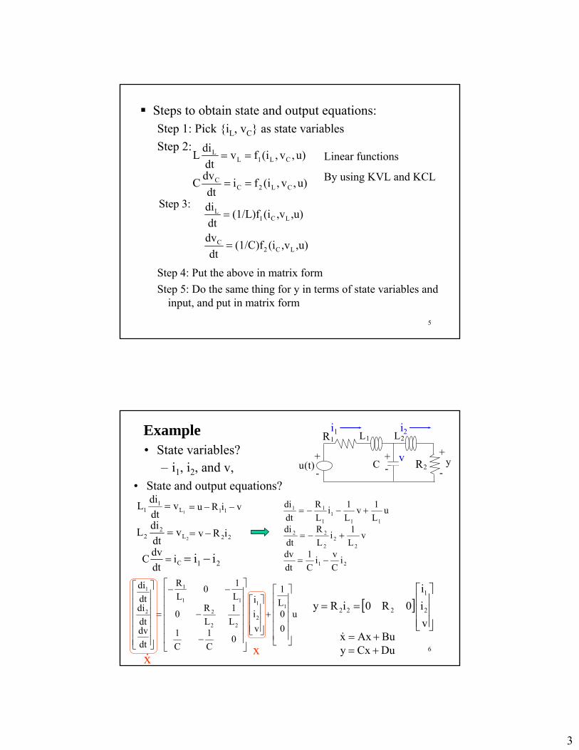
Steps to obtain state and output equations:Step 1: Pick {iL, vC} as state variablesStep 2:

u),v,(ifidt

dvC

u),v,(ifvdtdiL

CL2CC

CL1LL

==

== Linear functions

By using KVL and KCL

Step 3:L

1 C L

C2 C L

di (1/L)f (i ,v ,u)dtdv (1/C)f (i ,v ,u)dt

=

=

Step 4: Put the above in matrix formStep 5: Do the same thing for y in terms of state variables and

input, and put in matrix form

6

Example• State variables?

– i1, i2, and v,

++- - -

u(t) R2 C

L1

+ y

L2 R1i1

v

• State and output equations?

1L1

1 vdtdiL =

CidtdvC = 21

22

2

22

111

1

11

iCvi

C1

dtdv

vL1i

LR

dtdi

uL1v

L1i

LR

dtdi

−=

+−=

+−−=

u00L1

vii

0C1

C1

L1

LR0

L10

LR

dtdvdtdidtdi

1

2

1

22

2

11

1

2

1

⎥⎥⎥⎥⎥

⎦

⎤

⎢⎢⎢⎢⎢

⎣

⎡

+⎥⎥⎥

⎦

⎤

⎢⎢⎢

⎣

⎡

⎥⎥⎥⎥⎥⎥

⎦

⎤

⎢⎢⎢⎢⎢⎢

⎣

⎡

−

−

−−

=

⎥⎥⎥⎥⎥⎥

⎦

⎤

⎢⎢⎢⎢⎢⎢

⎣

⎡

i2

2L2

2 vdtdiL =

[ ]⎥⎥⎥

⎦

⎤

⎢⎢⎢

⎣

⎡==

vii

0R0iRy 2

1

222

viRu 11 −−=

22iRv −=

21 ii −=

x& x DuCxyBuAxx

+=+=&

4

7

• Elements: Spring, dashpot, and mass– Spring:

u(t)y(t)

M y(t), position,

positive direction

fS = Ky, opposite direction ~ Hooke’s law, K: Stiffness

– Dashpot: y(t), y'(t)

fD = Dy', opposite direction ~ D: Damping coefficient

– Mass: M, Newton’s law of motionNfyM =&& ~ Net force– LTI elements, LTI systems

– Linear differential equations with constant coefficients

Mechanical Systems

fN(t) y(t)

M

8

• Number of state variables? Which ones?– 2 state variables: x1 ≡ y, x2 ≡ x1'

u(t)y(t)

M

K

D

• How to describe the system? • Free body diagram:

u(t) y(t)

M Ky

Dy'

yDKyuyM &&& −−=

=1x& x2 =2x& =y&&M

DxKxuM

yDKyu 21 −−=

−− &

uM10

xx

MD

MK

10

dtdxdt

dx

2

1

2

1

⎥⎥⎦

⎤

⎢⎢⎣

⎡+⎥

⎦

⎤⎢⎣

⎡

⎥⎥⎦

⎤

⎢⎢⎣

⎡−−=

⎥⎥⎥

⎦

⎤

⎢⎢⎢

⎣

⎡1xy = [ ] 0u

xx

012

1 +⎥⎦

⎤⎢⎣

⎡=

uM1y

MKy

MDy =++ &&&

~ Input/Output description

5

9

• Steps to obtain state and output equations:Step 1: Determine ALL junctions and label the displacement

of each oneStep 2: Draw a free body diagram for each rigid body to obtain

the net force on itStep 3: Apply Newton's law of motion to each rigid body Step 4: Select the displacement and velocity as state variables,

and write the state and output equations in matrix form• For rotational systems: τ = Jα

• τ: Torque = Tangential force⋅arm• J: Moment of inertia = ∫r2dm • α: Angular acceleration

– There are also angular spring/damper

10

u(t)M

K D y1(t)

u(t)y1(t)

M

D(y1'-y2')(relative motion)

( )211 yyDuyM &&&& −−=

D(y2'-y1')

y2(t)

Ky2

y2(t)

( )122 yyDKy0 && −−−=

• Number of state variables? How to select the state variables?

231211 yx;yx;yx ≡≡≡ &

211 xyx =≡ &&

( )3212 xDDxuM1yx &&&& +−=≡

323 xDKxx −=&

uM1x

MK

3 +−=

u

0M10

x

DK10MK00

010x

⎥⎥⎥

⎦

⎤

⎢⎢⎢

⎣

⎡+

⎥⎥⎥⎥⎥

⎦

⎤

⎢⎢⎢⎢⎢

⎣

⎡

−

−=&

=⎥⎦

⎤⎢⎣

⎡=2

1yy

y u00

x100001

⎥⎦

⎤⎢⎣

⎡+⎥⎦

⎤⎢⎣

⎡

• How to describe the system?• How many junctions are there?

6

11

Example: an axial artificial heart pump

AMB Motor

AMB PMB Motor PMB

Indu

cer

Dif

fuse

r

PMB PMBAMB

AMB PM

PM

PM

PM

Illustration

12

PM

PM PM

PM

1F 2F3F

F1: the active force that can be generated as desired(F =k I1

2 / (c+y1)2 – kI22/(c-y1)2

F2, F3: passive forces, F2 = -k1y2, F3= -k3y3, similar to springs

I1

I2

y1y2y3

The forces acting on the rotor:

7

13

Modeling

1 11 1 12 2 1 1

2 21 1 22 2 2 1

y a y a y b Fy a y a y b F

= + += + +

&&

&&

1 2 3 1 2 2 1

1 1 2 2 3 3 2 1

, ( ) /, ( ) /

c cMy F F F y l y l y lJ l F l F l F y y lα α

= + + = += − + − = −

&&

&&

The motion of the rotor:

l1

y1

y2

yc

l2

F1 F3

F2

F2 and F3 depend on y1 and y2. Equation can be expressed in terms of y1 and y2

1 1 2 1 3 2 4 2Let , , ,x y x y x y x y= = = =& &

α

Center of massl3

14

1 1 2 1 3 2 4 2Let , , ,x y x y x y x y= = = =& &

1 1 2

2 1 11 1 12 3 1 1

3 2 4

4 2 21 1 22 3 2 1

x y xx y a x a x b Fx y xx y a x a x b F

= == = + += == = + +

& &

& &&

& &

& &&

11 12 11

21 22 2

0 1 0 0 00 0

0 0 0 1 00 0

=

a a bx x F

a a bAx Bu

⎡ ⎤ ⎡ ⎤⎢ ⎥ ⎢ ⎥

= +⎢ ⎥ ⎢ ⎥⎢ ⎥ ⎢ ⎥⎢ ⎥ ⎢ ⎥⎣ ⎦ ⎣ ⎦

+

&

1 11 1 12 2 1 1

2 21 1 22 2 2 1

y a y a y b Fy a y a y b F

= + += + +

&&

&&

In matrix form?

8

15

Integrator/Differentiator Realization• Elements: Amplifiers, differentiators, and integrators

Differentiator

f(t) y(t) = df/dts

Amplifier

f(t) y(t) = af(t)a

Integratorf(t)

y(t) =

1/s )t(yd)(f 0t

t0+∫ ττ

=τ

• Are they LTI elements? Yes• Which one has memory? What are their dimensions?

– Integrator has memory. Dimensions: 0, 0, and 1, respectively• They can be connected in various ways to form LTI

systems– Number of state variables = number of integrators– Linear differential equations with constant coefficients

16

• What are the state variables?

• Select output of integrators as SVs

2

1/s 1/s+

-u(t)

y(t)

x1x2

• What are the state and output equations?21 xx =&

12 x2ux −=& y = x2

u10

xx

0210

xx

2

1

2

1⎥⎦

⎤⎢⎣

⎡+⎥⎦

⎤⎢⎣

⎡⎥⎦

⎤⎢⎣

⎡−

=⎥⎦

⎤⎢⎣

⎡&

& [ ] u0xx

10y2

1 +⎥⎦

⎤⎢⎣

⎡=

A B C D

• Linear differential equations with constant coefficients

12 xx &&

9

17

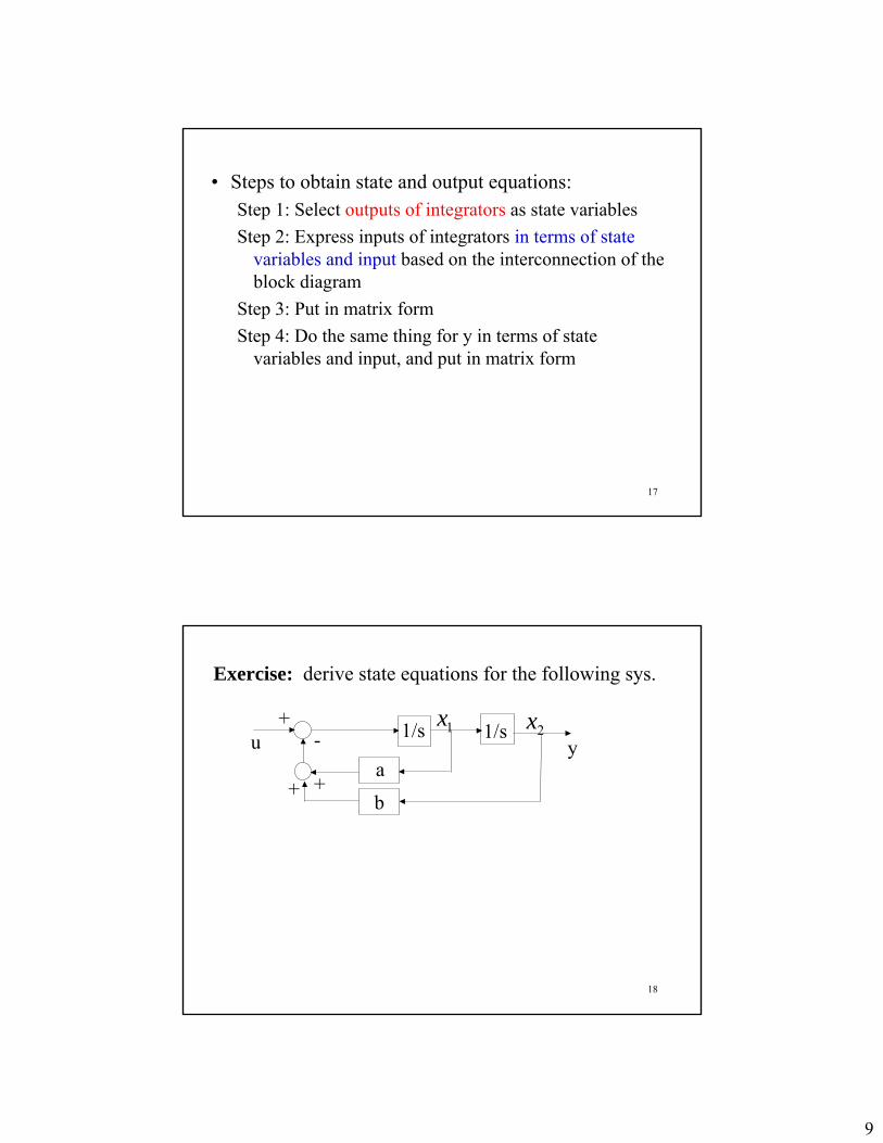
• Steps to obtain state and output equations:Step 1: Select outputs of integrators as state variablesStep 2: Express inputs of integrators in terms of state

variables and input based on the interconnection of the block diagram

Step 3: Put in matrix formStep 4: Do the same thing for y in terms of state

variables and input, and put in matrix form

18

a

b

u y

+ +

+

- 1/s 1/s

Exercise: derive state equations for the following sys.

2x1x

10

19

Operational Amplifiers (Op Amps)

• Usually, A > 104

– Ideal Op Amp:• A → ∝ ~ Implying that (va - vb) → 0, or va → vb

• ia → 0 and ib → 0 – Problem: How to analyze a circuit with ideal Op Amps

-Vcc, -15V

Non-inverting terminal, va

Inverting terminal, vb

Output, vo

ioia ib

Vcc, 15V

+

-

v0 = A (va - vb), with -VCC ≤ v0 ≤ VCC

-Vcc

va - vb

Slope = A

Vcc

Vo

20

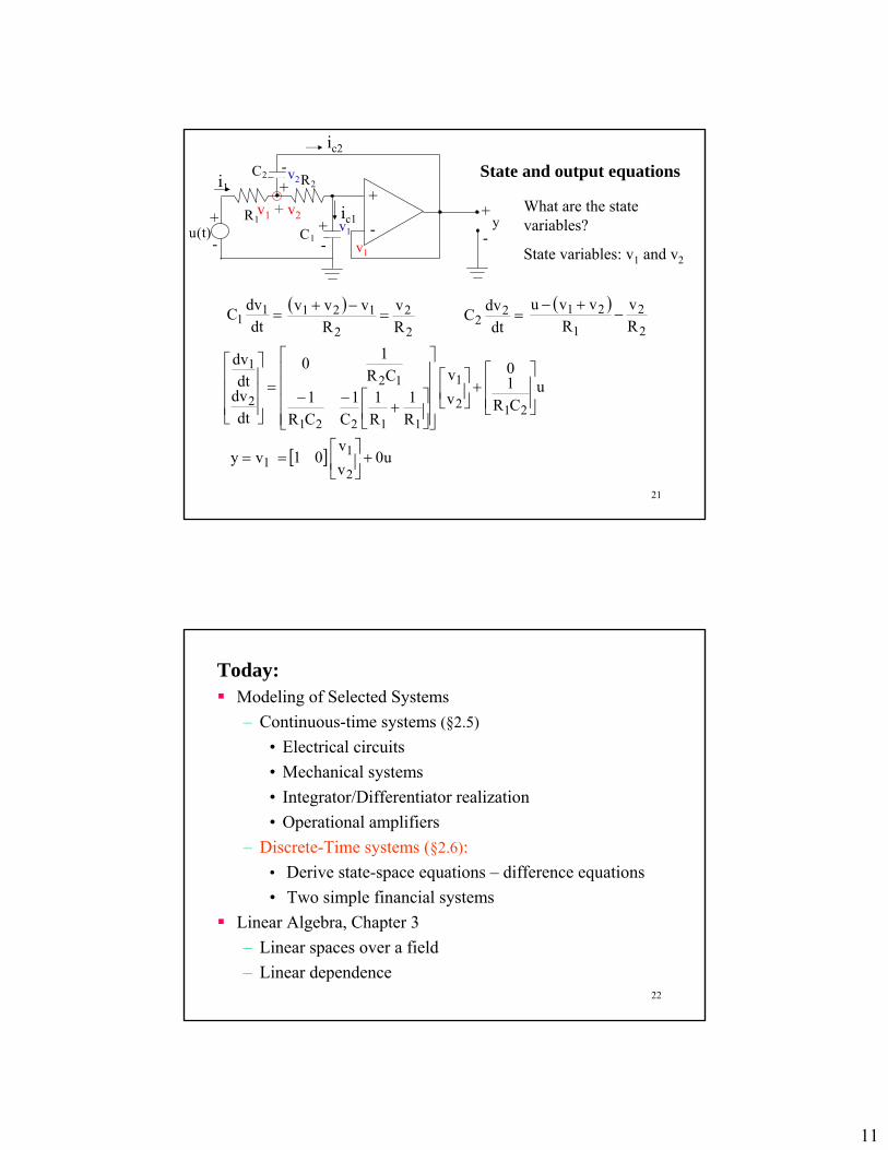
• Key ideas:– Make effective use of ia = ib = 0 and va = vb

– Do not apply the node equation to output terminals of op amps and ground nodes, since the output current and power supply current are generally unknown

+ u1(t)

R2R1

y u2(t)

+ +

-

- -

-

+i1

i2 i1 + i2 = 0

0R

uyR

uu2

2

1

21 =−

+−

21

21

1

2 uRR1u

RRy ⎟

⎠

⎞⎜⎝

⎛++−=

Delineate the relationship between input and outputInput/Output description

Pure gain, no SVs

u2

11

21

R2

R1

+ +

-+

u(t) -

-

y -

+

- + C1

C2

v1

v2 State and output equations

=dt

dvC 11

1vy =

v1 + v2What are the state variables?

State variables: v1 and v2

( )2

2

2

121Rv

Rvvv

=−+

=dt

dvC 22

( )2

2

1

21Rv

Rvvu

−+−

v1

uCR10

vv

R1

R1

C1

CR1

CR10

dtdvdt

dv

212

1

11221

122

1

⎥⎥⎦

⎤

⎢⎢⎣

⎡+⎥⎦

⎤⎢⎣

⎡

⎥⎥⎥⎥

⎦

⎤

⎢⎢⎢⎢

⎣

⎡

⎥⎦

⎤⎢⎣

⎡+

−−=

⎥⎥⎥

⎦

⎤

⎢⎢⎢

⎣

⎡

[ ] u0vv

012

1 +⎥⎦

⎤⎢⎣

⎡=

i1

ic2

ic1

22



– Discrete-Time systems (§2.6): • Derive state-space equations – difference equations• Two simple financial systems


12

23

2.6 Discrete-Time Systems• Thus far, we have considered continuous-time

systems and signals

t

y(t)

• In many cases signals are defined only at discrete instants of time

k

y[k]

T

– T: Sampling period– No derivative and no differential equations– The corresponding signal or system is described by

a set of difference equations

24

y[k] = u[k-1]

k

Elements: Amplifiers, delay elements, sources (inputs) Amplifiers:

u[k] y[k] = a u[k]a

~ LTI and memoryless

• Delay Element: u[k] y[k] = u[k-1]

z-1

~ LTI with memory (1 initial condition)They can be interconnected to form an LTI system

u[k]

k

13

25

Example

3

y[k]

Delay Delay

K

+ + - -

u[k]

• How to describe the above mathematically?– I/O description:

( ) or,]1k[Ky]1k[u]k[u3]k[y]1k[y −−−++−=+

]1k[u]k[u3]1k[Ky]k[y]1k[y −++−−−=+

y[k+1]

– A linear difference equation with constant coefficient

26

3

y[k]

Delay Delay

K

+ + - -

u[k]

State space description: Select output of delay elements as state variables

]k[u3]k[x]k[x]1k[x 211 ++−=+

]k[x]k[y 1=

]k[u]k[xK]1k[x 12 +−=+

x1[k]x1[k+1]x2[k]x2[k+1]

14

27

Two state variables, x1[k], x2[k]x1[k+1] = u[k] + x2[k]x2[k+1] = -bx1[k] + ax2[k]y[k] = x1[k]

u[k] +

+ z-1

a

y[k]+

-

z-1

b

x1[k]x1[k+1]

]k[u01

]k[xab10

]1k[x ⎥⎦

⎤⎢⎣

⎡+⎥⎦

⎤⎢⎣

⎡−

=+

x2[k]

[ ] ]k[x01]k[y =

x2[k+1]

Exercise:Derive state equations for the discrete-time system.

28

Example 1: Balance in your bank account

A bank offers interest r compounded every day at 12am– u[k]: The amount of deposit during day k

(u[k] < 0 for withdrawal)– y[k]: The amount in the account at the beginning

of day k What is y[k+1]?

y[k+1] = (1 + r) y[k] + u[k]

15

29

Example 2: Amortization

How to describe paying back a car loan over four years with initial debt D, interest r, and monthly payment p? Let x[k] be the amount you owe at the

beginning of the kth month. Thenx[k+1] = (1 + r) x[k] − p

Initial and terminal conditions: x[0] = D and final condition x[48] = 0 How to find p?

30

x[k+1] = (1 + r) x[k] + (−1) p The system:

Solution: A B u

pr

1r)(1Dr)(1pr)(1Dr)(1

1)p(r)(1x[0]r)(1

Bu[m]Ax[0]Ax[k]

kk

1k

0m

1mkk

1k

0m

1mkk

1k

0m

1mkk

−+−+=⎟

⎠

⎞⎜⎝

⎛+−+=

−+++=

+=

∑

∑

∑

−

=

−−

−

=

−−

−

=

−−

Given D=20000; r=0.004; x[48]=0;

p0.004

1)004.0(100002)004.0(10 48

48 −+−+= p=458.7761

Your monthlypayment

16

31



– Discrete-Time systems (§2.6):• Derive state-space equations – difference equations• Two simple financial systems


32

Our modeling efforts lead to a state-space description of LTI system


+=+=&

]k[Du]k[Cx]k[y]k[Bu]k[Ax]1k[x

+=+=+

Analysis problems: stability; transient performances;potential for improvement by feedback control, …

Linear Algebra: Tools for System Analysis and Design

17

33

• Consider an LTI continuous-time system


+=+=&

• For a practical system, usually there is a natural way to choose the state variables, e.g.,

⎥⎦

⎤⎢⎣

⎡=

2

1

xx

x iL

vc• However, the natural state selection may not be the

best for analysis. There may exist other selection tomake the structure of A,B,C,D simple for analysis

• If T is a nonsingular matrix, then z = Tx is also the state and satisfies

Du(t)z(t)CTy(t)TBu(t)z(t)TAT(t)z

1

1

+=+=

−

−&

u(t)D~z(t)C~y(t)u(t)B~z(t)A~(t)z

+=+=&

34

• Two descriptions


+=+=&


+=+=&

are equivalent when I/O relation is concerned. • For a particular analysis problem, a special form of

D~,C~,B~,A~ may be the most convenient, e.g.,

[ ]001C~

,100

B~,aaa100010

A~,λ000λ000λ

A~

3213

2

1

=

⎥⎥⎥

⎦

⎤

⎢⎢⎢

⎣

⎡=

⎥⎥⎥

⎦

⎤

⎢⎢⎢

⎣

⎡=

⎥⎥⎥

⎦

⎤

⎢⎢⎢

⎣

⎡=

• We need to use tools from Linear Algebra to get a desirable description.

18

35

The operation x → z = Tx is called a lineartransformation. It plays the essential role in obtaining a desired

state-space description


+=+=&

Linear algebra will be needed for the transformationand analysis of the system– Linear spaces over a vector field– Relationship among a set of vectors: LD and LI– Representations of a vector in terms of a basis– The concept of perpendicularity: Orthogonality– Linear Operators and Representations

36

3.1 Linear Vector Spaces and Linear Operators

Rn: n-dimensional real linear vector spaceCn: n-dimensional complex linear vector spaceRn×m: the set of n×m real matrices (also a vector space)Cn×m: the set of n×m complex matrices (a vector space)

Notation:

A matrix T∈Rn×m represents a linear operation fromRm to Rn: x∈Rm → Tx∈Rn.

All the matrices A,B,C,D in the state space equationare real

19

37

Linear Vector Spaces Rn and Cn

R: The set of real numbers; C: The set of complex numbersIf x is a real number, we say x∈R; If x is a complex number, we say x∈CRn: n-dimensional real vector spaceCn: n-dimensional complex vector space

1

n 21 2R : , , , R ,n

n

xxx x x x

x

⎧ ⎫⎡ ⎤⎪ ⎪⎢ ⎥⎪ ⎪= = ∈⎨ ⎬⎢ ⎥⎪ ⎪⎢ ⎥

⎢ ⎥⎪ ⎪⎣ ⎦⎩ ⎭

LM

1

n 21 2C : , , , Cn

n

xxx x x x

x

⎧ ⎫⎡ ⎤⎪ ⎪⎢ ⎥⎪ ⎪= = ∈⎨ ⎬⎢ ⎥⎪ ⎪⎢ ⎥

⎢ ⎥⎪ ⎪⎣ ⎦⎩ ⎭

LM

If x,y∈Rn, a,b∈R, then ax + by∈Rn Rn is a linear space.

If x,y∈Cn, a,b∈C, then ax + by∈Cn Cn is a linear space.

38

SubspaceConsider Y ⊂ Rn. Y is a subspace of Rn iff Y itself is a linear space– Y is a subspace iff α1y1 + α2y2 ∈ Y for all y1, y2 ∈ Y

and α1, α2 ∈ R (linearity condition)– Subspace of Cn can be defined similarly

11 2 1 2

2: 2 1 0, , RxY x x x xx

⎧ ⎫⎡ ⎤= − + = ∈⎨ ⎬⎢ ⎥⎣ ⎦⎩ ⎭

Is the linearity condition satisfied?

Example: Consider R2. The set of (x1,x2) satisfying x1 - 2x2 + 1 = 0 can be written as

20

39

Then how about the set of (x1,x2) satisfying x1 - 2x2 = 0?

– Yes. In fact, any straight line passing through 0 form a subspace

What would be a subspace for R3 ?– Any plane or straight line passing through 0

{(x1,x2,x3): ax1+bx2+cx3=0} for constants a,b,c denote a plane. How to represent a line in the space?

The set of solutions to a system of homogeneous equation is a subspace: {x ∈Rn: Ax=0}. How about {x ∈Rn: Ax=c} ?

Y: x1-2x2=0

x1

x2

11 2 1 2

2: 2 0, , RxY x x x xx

⎧ ⎫⎡ ⎤= − = ∈⎨ ⎬⎢ ⎥⎣ ⎦⎩ ⎭

40

Consider Rn, – Given any set of vectors {xi}i=1 to n, xi ∈Rn. – Form the set of linear combinations

⎭⎬⎫

⎩⎨⎧

∈≡ ∑=

Rα :xαY i

n

1iii

– Then Y is a linear space, and is a subspace of Rn.– It is the space spanned by {xi}i=1 to n

21

41

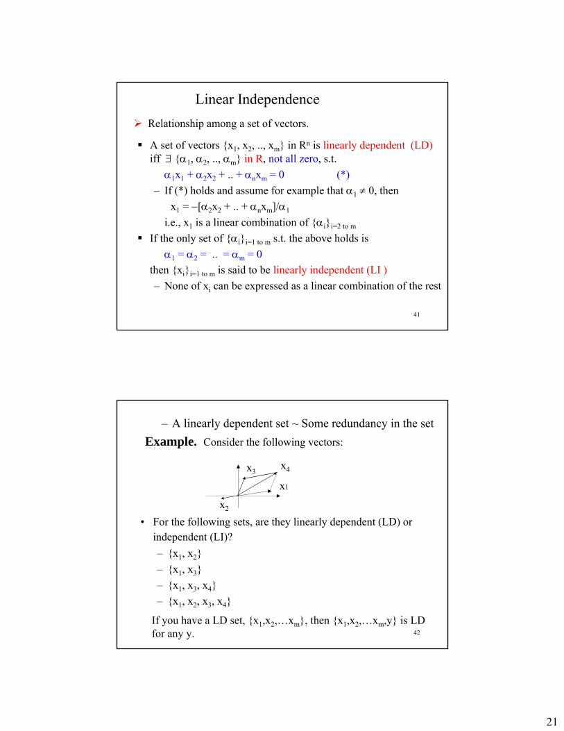
Linear Independence

A set of vectors {x1, x2, .., xm} in Rn is linearly dependent (LD)iff ∃ {α1, α2, .., αm} in R, not all zero, s.t.

α1x1 + α2x2 + .. + αnxm = 0 (*)– If (*) holds and assume for example that α1 ≠ 0, then

x1 = −[α2x2 + .. + αnxm]/α1

i.e., x1 is a linear combination of {αi}i=2 to m

If the only set of {αi}i=1 to m s.t. the above holds isα1 = α2 = .. = αm = 0

then {xi}i=1 to m is said to be linearly independent (LI )– None of xi can be expressed as a linear combination of the rest

Relationship among a set of vectors.

42

– A linearly dependent set ~ Some redundancy in the setExample. Consider the following vectors:

x1

x2

x3x4

• For the following sets, are they linearly dependent (LD) or independent (LI)?– {x1, x2}– {x1, x3}– {x1, x3, x4}– {x1, x2, x3, x4}

If you have a LD set, {x1,x2,…xm}, then {x1,x2,…xm,y} is LDfor any y.

22

43

• A general way to detect LD or LI:– {x1, x2, .., xm} are LD iff ∃ {α1, α2, .., αm}, not all

zero, s.t. α1x1 + α2x2 + .. + αmxm= 0

[ ] ,0

α:αα

x...xxxαxαxα

m

2

1

m21mm2211 =⎥⎥⎥

⎦

⎤

⎢⎢⎢

⎣

⎡

=+++ L

• Given a set of vectors, {x1,x2,…,xm}⊂ Rn, how to findout if there are LD or LI?

= A∈Rn×m = α∈Rm

Aα = 0

– {x1, x2, .., xm} are LD iff Aα =0 has a nonzero solution

Need to understand the solution to a homogeneous equation. There is always a solution α = 0. Question: under what condition is the solution unique?

44

Given {x1, x2, .., xm}, form [ ]1 2 mA x x ... x=

Aα = 0

• If n=m and A is singular, det(A)= 0, rank(A) < m ∃ α≠0 s.t. Aα=0, hence LD

Detecting LD and LI through solutions to linear equations

Consider the equation

If the equation has a unique solution, LI;If the equation has nonunique solution, LD.

This is related to the rank of A.

If rank(A)=m, (A has full column rank), the solution is unique;If rank(A)<m, the solution is not unique.

• If n=m and A is nonsingular, det(A)≠ 0, rank(A)=monly α=0 satisfies. Aα=0, hence LI

23

45

• Are the following vectors LD or LI?

⎥⎥⎥

⎦

⎤

⎢⎢⎢

⎣

⎡=

⎥⎥⎥

⎦

⎤

⎢⎢⎢

⎣

⎡=

⎥⎥⎥

⎦

⎤

⎢⎢⎢

⎣

⎡=

741

x,521

x,432

x 321

LI010754423112

A)det( ≠−==

• How about

⎥⎥⎥

⎦

⎤

⎢⎢⎢

⎣

⎡=

⎥⎥⎥

⎦

⎤

⎢⎢⎢

⎣

⎡=

⎥⎥⎥

⎦

⎤

⎢⎢⎢

⎣

⎡=

654

x,432

x,321

x 321

643532421

)Adet( =

0202436323018

145622433442352163

=−−−++=

××−××−××−××+××+××=

LD

det(A)=?

46

• All depends on the uniqueness of solution for Aα=0• If m> n, A is a wide matrix, rank(A)<m, always has a

nonzero solution, e.g.,

⎥⎦

⎤⎢⎣

⎡−

=⎥⎦

⎤⎢⎣

⎡=⎥

⎦

⎤⎢⎣

⎡=⎥

⎦

⎤⎢⎣

⎡−

=211101

A,21

x,10

x,1

1x 321

If m < n and rank(A) = m, LI;If m < n and rank(A)<m, LD;

,1111

00,

110110

21⎥⎥⎦

⎤

⎢⎢⎣

⎡

−−=

⎥⎥⎦

⎤

⎢⎢⎣

⎡= AA

rank(A1)=2=m, LI rank(A2)=1<m, LD

A m

n

m

n A

24

47

• Examples: determine the LD/LI for the following group of vectors

sin cos, ,cos sin

sin cos,cos sin

θ θθ θ

θ θθ θ

⎧ ⎫−⎡ ⎤ ⎡ ⎤⎨ ⎬⎢ ⎥ ⎢ ⎥⎣ ⎦ ⎣ ⎦⎩ ⎭⎧ ⎫⎡ ⎤ ⎡ ⎤⎨ ⎬⎢ ⎥ ⎢ ⎥⎣ ⎦ ⎣ ⎦⎩ ⎭

1 1 1, , ,0 1 3

1 01 , 11 3

1 0 21 , 1 , 31 3 5

⎧ ⎫⎡ ⎤ ⎡ ⎤ ⎡ ⎤⎨ ⎬⎢ ⎥ ⎢ ⎥ ⎢ ⎥⎣ ⎦ ⎣ ⎦ ⎣ ⎦⎩ ⎭⎧ ⎫⎡ ⎤ ⎡ ⎤⎪ ⎪⎢ ⎥ ⎢ ⎥⎨ ⎬

⎢ ⎥ ⎢ ⎥⎪ ⎪⎣ ⎦ ⎣ ⎦⎩ ⎭⎧ ⎫⎡ ⎤ ⎡ ⎤ ⎡ ⎤⎪ ⎪⎢ ⎥ ⎢ ⎥ ⎢ ⎥⎨ ⎬

⎢ ⎥ ⎢ ⎥ ⎢ ⎥⎪ ⎪⎣ ⎦ ⎣ ⎦ ⎣ ⎦⎩ ⎭

48

Dimension

• For a linear vector space, the maximum number of LI vectors is called the dimension of the space, denoted as D

• Consider {x1,x2,…,xm}⊂ Rn

If m>n, they are always dependent, D ≤ n For m=n, there exist x1,x2,…xn such that

with A=[x1,x2,…xn], |A|≠0, xi’s LI, D ≥ n Hence D = n

25

49


• Electrical circuits, Mechanical systems• Integrator/Differentiator realization• Operational amplifiers

– Discrete-Time systems (§2.6): • Derive state-space equations – difference equations• Two simple financial systems


Next time: Linear algebra continued.

50

C

RL

Input u=Vin Output: y =Vo,

-+

R

2. Derive state-space description for the diagram:

1. Derive state-space description for the circuit:

u y

−+

+- 1/s1/s 1/s

a

b

c+

+

Homework Set #3

+ vc −

iL

+

−

+

−

26

51

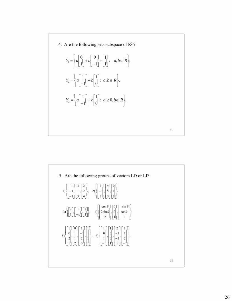
4. Are the following sets subspace of R2 ?

.,0:01

11

,,:01

11

,,:11

10

10

2

2

1

⎭⎬⎫

⎩⎨⎧

∈≥⎥⎦

⎤⎢⎣

⎡+⎥

⎦

⎤⎢⎣

⎡−

=

⎭⎬⎫

⎩⎨⎧

∈⎥⎦

⎤⎢⎣

⎡+⎥

⎦

⎤⎢⎣

⎡−

=

⎭⎬⎫

⎩⎨⎧

∈⎥⎦

⎤⎢⎣

⎡+⎥

⎦

⎤⎢⎣

⎡−

+⎥⎦

⎤⎢⎣

⎡=

RbabaY

RbabaY

RbabaY

52

5. Are the following groups of vectors LD or LI?

⎪⎭

⎪⎬

⎫

⎪⎩

⎪⎨

⎧

⎥⎥⎥

⎦

⎤

⎢⎢⎢

⎣

⎡−

⎥⎥⎥

⎦

⎤

⎢⎢⎢

⎣

⎡

⎥⎥⎥

⎦

⎤

⎢⎢⎢

⎣

⎡

⎭⎬⎫

⎩⎨⎧

⎥⎦

⎤⎢⎣

⎡⎥⎦

⎤⎢⎣

⎡−⎥

⎦

⎤⎢⎣

⎡

⎪⎭

⎪⎬

⎫

⎪⎩

⎪⎨

⎧

⎥⎥⎥

⎦

⎤

⎢⎢⎢

⎣

⎡

⎥⎥⎥

⎦

⎤

⎢⎢⎢

⎣

⎡

⎥⎥⎥

⎦

⎤

⎢⎢⎢

⎣

⎡−

⎪⎭

⎪⎬

⎫

⎪⎩

⎪⎨

⎧

⎥⎥⎥

⎦

⎤

⎢⎢⎢

⎣

⎡

⎥⎥⎥

⎦

⎤

⎢⎢⎢

⎣

⎡

⎥⎥⎥

⎦

⎤

⎢⎢⎢

⎣

⎡

−−

1cossin

,100

,2

sin2cos

)4,12

,1

,1

)3

110

,0

,11

1)2,

422

,313

,11

1)1

θθ

θθ

aa

ba

,

1211

,

111

2

,

1001

,

1101

)6,

1111

,

021

1

,

2110

,

1201

)5

⎪⎪⎭

⎪⎪⎬

⎫

⎪⎪⎩

⎪⎪⎨

⎧

⎥⎥⎥⎥

⎦

⎤

⎢⎢⎢⎢

⎣

⎡

−⎥⎥⎥⎥

⎦

⎤

⎢⎢⎢⎢

⎣

⎡

−−

⎥⎥⎥⎥

⎦

⎤

⎢⎢⎢⎢

⎣

⎡

⎥⎥⎥⎥

⎦

⎤

⎢⎢⎢⎢

⎣

⎡

−⎪⎪⎭

⎪⎪⎬

⎫

⎪⎪⎩

⎪⎪⎨

⎧

⎥⎥⎥⎥

⎦

⎤

⎢⎢⎢⎢

⎣

⎡

⎥⎥⎥⎥

⎦

⎤

⎢⎢⎢⎢

⎣

⎡−

⎥⎥⎥⎥

⎦

⎤

⎢⎢⎢⎢

⎣

⎡

⎥⎥⎥⎥

⎦

⎤

⎢⎢⎢⎢

⎣

⎡

16.513 Control Systems - Faculty Server Contactfaculty.uml.edu/thu/controlsys/note03.pdf–...

Documents

Transcript of 16.513 Control Systems - Faculty Server Contactfaculty.uml.edu/thu/controlsys/note03.pdf–...