16 - University of Arizonakcreath/pdf/pubs/2007_KC_JS_JC… · · 2010-03-0316.1. MOIRE´ AND...

16

Optical Metrology of Diffuse Surfaces

K. CreathCollege of Optical Sciences, University of Arizona, Tucson, AZ 85721

Optineering, 2247 E La Mirada St, Tucson, AZ 85719

J. SchmitVeeco Tucson, Inc, 2650 E Elvira Rd, Tucson, AZ 85706

J. C. WyantCollege of Optical Sciences, University of Arizona, Tucson, AZ 85721

This chapter discusses moire, fringe projection, structured illumination, holographic

interferometry, digital holography, and speckle interferometry techniques for testing

diffuse surfaces. Diffuse surfaces may be ground optical surfaces; or more often than

not, they are other types of engineering surfaces or human figures. The main

applications of these techniques are to determine surface form and shape or to

measure displacement due to stress and object motion. When measuring surface

form, these techniques provide a coarser and more flexible means of testing a wider

variety of surfaces than do conventional interferometers. For displacement measure-

ment due to applied stress, static as well as time-average and dynamic displacements

can be determined quantitatively. These techniques are used a lot in machine vision

applications, for process control, and for specialized measurement tasks on engineer-

ing components. Applications range from measuring the shape of an airplane

window to determining whether components will stay on a circuit board, to studying

vibration modes of turbine blades, to monitoring the alignment of segments in a large

segmented telescope, to making replicas of historic sculptures, producing a well-

fitting pair of jeans, and creating animated movies or video games with realistic

motion of live figures. The newest techniques pushing the limits of this technology

currently focus on rapid prototyping and real-time shape observation for multimedia

and security.

Optical Shop Testing, Third Edition Edited by Daniel Malacara

Copyright # 2007 John Wiley & Sons, Inc.

764

16.1. MOIRE AND FRINGE PROJECTION TECHNIQUES

16.1.1. Introduction

The term moire is not the name of a person; in fact, it is a French word referring to

‘‘an irregular wavy finish usually produced on a fabric by pressing between engraved

rollers’’ (Webster’s, 1981). In optics, it refers to a beat pattern produced between two

gratings of approximately equal spacing. It can be seen in everyday things, such as

the overlapping of two window screens, the rescreening of a half-tone picture, or with

a striped shirt seen on television. The use of moire for reduced sensitivity testing was

introduced by Lord Rayleigh in 1874. Lord Rayleigh looked at the moire between

two identical gratings to determine their quality even though each individual grating

could not be resolved under a microscope.

Fringe projection entails projecting a fringe pattern or grating on an object and

viewing it from a different direction. The first use of fringe projection for determining

surface topography was presented by Rowe and Welford in 1967. It is a convenient

technique for contouring objects which are too coarse to be measured with standard

interferometry. Fringe projection is related to optical triangulation using a single

point of light and light sectioning where a single line is projected onto an object and

viewed in a different direction to determine the surface contour (Case et al., 1987).

These techniques are usually used with diffuse objects; however, alternative methods

have been developed to measure specular surfaces by looking at the fringe reflection

(Ritter and Hahn, 1983; Hang et al., 2000).

Moire and fringe projection interferometry complement conventional holographic

interferometry, especially for testing optics to be used at long wavelengths. Although

two-wavelength holography (TWH) can be used to contour surfaces at any longer-

than-visible wavelength, visible interferometric environmental conditions are

required. Moire and fringe projection interferometry can contour surfaces at any

wavelength longer than 10–100 mm with reduced environmental requirements and no

intermediate photographic recording setup. Moire is also a useful technique for

aiding in the understanding of interferometry.

This chapter explains what moire is and how it relates to interferometry. Contour-

ing techniques utilizing fringe projection, projection and shadow moire, and two-

angle holography are all described and compared. All of these techniques provide the

same result and can be described by a single theory. The relationship between these

techniques and the holographic and conventional interferometry will be shown. Errors

caused by divergent geometries are described, and applications of these techniques

combined with phase-measurement techniques are presented. Further information on

these techniques can be found in the following books and book chapters: Varner

(1974), Vest (1979), Hariharan (1996), Gasvik (2002), Chiang (1983) and Patorski and

Kujawinska, (1993), Post et al. (1997), Amridror (2000), and Walker (2004).

16.1.2. What is Moire?

Moire patterns are extremely useful to help understand basic interferometry and

interferometric test results. Figure 16.1 shows the moire pattern (or beat pattern)

Q1

Q1

16.1. MOIRE AND FRINGE PROJECTION TECHNIQUES 765

produced by two identical straight line gratings rotated by a small angle relative to

each other. A dark fringe is produced where the dark lines are out of step one-half

period, and a bright fringe is produced where the dark lines for one grating fall on top

of the corresponding dark lines for the second grating. If the angle between the two

gratings is increased, the separation between the bright and dark fringes decreases.

(A simple explanation of moire is given by Oster and Nishijima (1963).)

If the gratings are not identical to the straight line gratings, the moire pattern

(bright and dark fringes) will not be straight equi-spaced fringes. The following

analysis shows how to calculate the moire pattern for arbitrary gratings. Let the

intensity transmission function for two gratings f1ðx; yÞ and f2ðx; yÞ be given by

f1ðx; yÞ ¼ a1 þX1n¼1

b1n cos½nf1ðx; yÞ�

f2ðx; yÞ ¼ a2 þX1m¼1

b2m cos½mf2ðx; yÞ�ð16:1Þ

where f(x,y) is the function describing the basic shape of the grating lines. For the

fundamental frequency, f(x,y) is equal to an integer times 2p at the center of each

bright line and is equal to an integer plus one-half times 2p at the center of each dark

line. The b coefficients determine the profile of the grating lines (i.e., square wave,

triangular, sinusoidal, etc). For a sinusoidal line profile, bi1 is the only nonzero term.

When these two gratings are superimposed, the resulting intensity transmission

function is given by the product

f1ðx; yÞf2ðx; yÞ ¼ a1a2 þ a1

X1m¼1

b2m cos½mf2ðx; yÞ� þ a2

X1n¼1

b1n cos½nf1ðx; yÞ�

þX1m¼1

X1n¼1

b1nb2m cos½nf1ðx; yÞ� cos½mf2ðx; yÞ�: ð16:2Þ

2 a

Destructive interference

Constructive interference

l /2 sin a

Observation plane

(a) (b)

y

x

FIGURE 16.1. (a) Straight line grating. (b) Moire between two straight line gratings of the same pitch at

an angle 2a with respect to one another.

766 OPTICAL METROLOGY OF DIFFUSE SURFACES

The first three terms of Eq. (16.2) provide information which can be determined by

looking at the two patterns separately. The last term is the interesting one, and can be

rewritten as

Term 4 ¼ 1

2b11b21 cos½f1ðx; yÞ � f2ðx; yÞ�

þ 1

2

X1m¼1

X1n¼1

b1nb2m cos½nf1ðx; yÞ � mf2ðx; yÞ�; n and m both 6¼ 1

þ 1

2

X1m¼1

X1n¼1

b1nb2m cos½nf1ðx; yÞ þ mf2ðx; yÞ� ð16:3Þ

This expression shows that by superimposing the two gratings, the sum and differ-

ence between the two gratings is obtained. The first term of Eq. (16.3) represents the

difference between the fundamental pattern making up the two gratings. It can be

used to predict the moire pattern shown in Figure 16.1. Assuming that two gratings

are oriented with an angle 2a between them with the y axis of the coordinate system

bisecting this angle, the two grating functions f1ðx; yÞ and f2ðx; yÞ can be written as

f1ðx; yÞ ¼2pl1

ðx cos aþ y sin aÞ

and

f2ðx; yÞ ¼2pl2

ðx cos a� y sin aÞ ð16:4Þ

where l1 and l2 are the line spacings of the two gratings. Equation (16.4) can be

rewritten as

f1ðx; yÞ � f2ðx; yÞ ¼2plbeat

x cos aþ 4p

ly sin a ð16:5Þ

where l ¼ ðl1 þ l2Þ=2 is the average line spacing, and lbeat is the beat wavelength

between the two gratings given by

lbeat ¼l1l2

l2 � l1

ð16:6Þ

Note that this beat wavelength is the same that was obtained for two-wavelength

interferometry as described in Chapter 15, and is also referred to as the synthetic or

equivalent wavelength. Using Eq. (16.3), the moire or beat will be lines whose

centers satisfy the equation

f1ðx; yÞ � f2ðx; yÞ ¼ M2p ð16:7Þ

Three separate cases for moire fringes can be considered.


For the first case l1 ¼ l2 ¼ l. The first term of Eq. (16.5) is zero, and the fringe

centers are given by

Ml ¼ 2y sin a ð16:8Þ

where M is an integer corresponding to the fringe order (see Fig. 16.2(a)). As was

expected, Eq. (16.8) is the equation of equi-spaced horizontal lines as seen in

Fig. 16.1.

For the second simple case l1 6¼ l2 and the gratings are parallel to each other with

a ¼ 0. This makes the second term of Eq. (16.5) vanish. The moire will then be lines

which satisfy

Mlbeat ¼ x ð16:9Þ

These fringes are equally-spaced lines parallel to the grating lines (see Fig. 16.2(b)).

For the third and more general case where the two gratings have different line

spacings l1 6¼ l2 and the angle between the gratings is nonzero a 6¼ 0, the equation

for the moire fringes will now be

Ml ¼ llbeat

x cos aþ 2y sin a ð16:10Þ

This is the equation of straight lines whose spacing and orientation is dependent upon

the relative difference between the two grating spacings and the angle between the

gratings (see Fig. 16.2(c)).

The orientation and spacing of the moire fringes for the general case can be

determined from the geometry shown in Figure. 16.3 (Chiang, 1983). The distance

AB can be written in terms of the two grating spacings,

AB ¼ l1

sinðy� aÞ ¼l2

sinðyþ aÞ ð16:11Þ

FIGURE 16.2. Moire patterns caused by two straight line gratings with (a) the same pitch tilted with

respect to one another, (b) different frequencies and no tilt, and (c) different frequencies tilted with respect to

one another.


where y is the angle the moire fringes make with the y axis. After rearranging, the

fringe orientation angle y is given by

tan y ¼ tan al1 þ l2

l2 � l1

� �ð16:12Þ

When a ¼ 0 and l1 6¼ l2, y ¼ 0�, and when l1 ¼ l2 with a 6¼ 0, y ¼ 90� as

expected. The fringe spacing perpendicular to the fringe lines can be found by

equating quantities for the distance DE,

DE ¼ l1

sin 2a¼ C

sinðyþ aÞ ð16:13Þ

where C is the fringe spacing or contour interval. This can be rearranged to yield

C ¼ l1

sinðyþ aÞsin 2a

� �ð16:14Þ

By substituting for the fringe orientation y, the fringe spacing can be found in terms

of the grating spacings and angle between the gratings;

C ¼ l1l2ffiffiffiffiffiffiffiffiffiffiffiffiffiffiffiffiffiffiffiffiffiffiffiffiffiffiffiffiffiffiffiffiffiffiffiffiffiffiffiffiffiffiffiffiffiffiffiffiffiffiffiffiffiffiffiffiffil2

2 sin2 2aþ ðl2 cos 2a� l1Þ2q ð16:15Þ

In the limit that a ¼ 0 and l1 6¼ l2, the fringe spacing equals lbeat, and in the limit

that l1 ¼ l2 ¼ l and a 6¼ 0, the fringe spacing equals l=ð2 sin aÞ. It is possible to

determine l2 and a from the measured fringe spacing and orientation as long as l1 is

known (Chiang, 1983).

x

y

λ1λ2

Moiréfringes

Gratings

C

DA

B

θ θ

a a

E

FIGURE 16.3. Geometry used to determine spacing and angle of moire fringes between two gratings of

different frequencies tilted with respect to one another.

Q1


16.1.3. Moire and Interferograms

Now that we have covered the basic mathematics of moire patterns, let us see how

moire patterns are related to interferometry. The single grating shown in Figure 16.1

can be thought of as a ‘‘snapshot’’ of plane waves (like in a collimated beam)

traveling to the right where the distance between the grating lines is equal to the

wavelength of light. Superimposing the two sets of grating lines in Fig. 16.1b can be

thought of as superimposing two plane waves with an angle of 2a between their

directions of propagation. When the two waves are in phase, bright fringes result

(constructive interference) and when they are out of phase, dark fringes result

(destructive interference). For a collimated plane wave, the ‘‘grating’’ lines are really

planes (sheets) perpendicular to the plane of the figure and the dark and bright fringes

are also planes perpendicular to the plane of the figure. If the plane waves are

traveling to the right, these fringes would be observed by placing a screen perpendi-

cular to the plane of the figure and to the right of the grating lines as shown in

Figure 16.1. The spacing of the interference fringes on the screen is given by

Eq. (16.8), where l is now the wavelength of light. Thus, the moire of two

straight-line gratings correctly predicts the centers of the interference fringes pro-

duced by interfering two plane waves. Since the gratings used to produce the moire

pattern are binary gratings, the moire does not correctly predict the sinusoidal

intensity profile of the interference fringes. (If both gratings had sinusoidal intensity

profiles, the resulting moire would still not have a sinusoidal intensity profile because

of higher-order terms.)

More complicated gratings, such as circular gratings, can also be investigated.

Figure 16.4(b) shows the superposition of two identical circular grating patterns

shown in Figure 16.4(a). This composite pattern indicates the fringe positions

obtained by interfering two spherical wavefronts. The centers of the two circular

gratings can be considered the source locations for two spherical waves. Just as for

two plane waves, the spacing between the grating lines is equal to the wavelength of

light. When the two patterns are in phase, bright fringes are produced, and when the

patterns are completely out of phase, dark fringes result. For a point on a given

fringe, the difference in the distances from the two source points and the fringe point

is a constant. Hence, the fringes are hyperboloids. Due to symmetry, the fringes seen

on observation plane A of Figure 16.4(b) must be circular. (Plane A is along the top

of Fig. 16.4(b) and perpendicular to the line connecting the two sources as well as

perpendicular to the page.) Figure 16.4(c) shows a representation of these inter-

ference fringes and represents the interference pattern obtained by interfering a non-

tilted plane wave and a spherical wave. (A plane wave can be thought of as a

spherical wave with an infinite radius of curvature.) Figure 16.4(d) shows that the

interference fringes in plane B are essentially straight equi-spaced fringes going into

the page. (These fringes are strictly speaking still hyperbolas, but in the limit of large

distances, they are essentially straight lines. Plane B is along the side of Fig. 16.4(b)

and parallel to the line connecting the two sources as well as perpendicular to

the page.)


FIGURE 16.4. Interference of two spherical waves. (a) Circular line grating representing a spherical

wavefront. (b) Moire pattern obtained by superimposing two circular line patterns. (c) Fringes observed in

plane A. (d) Fringes observed in plane B.


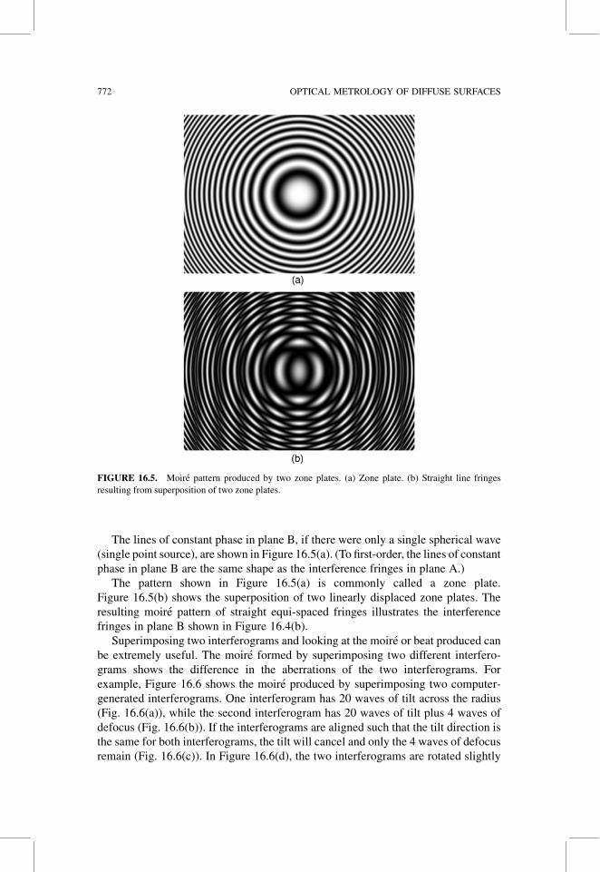
The lines of constant phase in plane B, if there were only a single spherical wave

(single point source), are shown in Figure 16.5(a). (To first-order, the lines of constant

phase in plane B are the same shape as the interference fringes in plane A.)

The pattern shown in Figure 16.5(a) is commonly called a zone plate.

Figure 16.5(b) shows the superposition of two linearly displaced zone plates. The

resulting moire pattern of straight equi-spaced fringes illustrates the interference

fringes in plane B shown in Figure 16.4(b).

Superimposing two interferograms and looking at the moire or beat produced can

be extremely useful. The moire formed by superimposing two different interfero-

grams shows the difference in the aberrations of the two interferograms. For

example, Figure 16.6 shows the moire produced by superimposing two computer-

generated interferograms. One interferogram has 20 waves of tilt across the radius

(Fig. 16.6(a)), while the second interferogram has 20 waves of tilt plus 4 waves of

defocus (Fig. 16.6(b)). If the interferograms are aligned such that the tilt direction is

the same for both interferograms, the tilt will cancel and only the 4 waves of defocus

remain (Fig. 16.6(c)). In Figure 16.6(d), the two interferograms are rotated slightly

FIGURE 16.5. Moire pattern produced by two zone plates. (a) Zone plate. (b) Straight line fringes

resulting from superposition of two zone plates.


with respect to each other so that the tilt will not quite cancel. These results can be

described mathematically by looking at the two grating functions:

f1ðx; yÞ ¼ 2pð20r cosjþ 4r2Þ

and

f2ðx; yÞ ¼ 2p½20r cosðjþ aÞ� ð16:16Þ

A bright fringe is obtained when

f1 � f2

2p¼ 20r½cosj� cosðjþ aÞ� þ 4r2 ¼ M ð16:17Þ

If a ¼ 0, the tilt cancels completely and 4 waves of defocus remain; otherwise, some

tilt remains in the moire pattern.

Figure 16.7 shows similar results for interferograms containing third-order aber-

rations. A computer-generated interferogram having 22 waves of tilt across the

radius, 4 waves of spherical and �2 waves of defocus is shown in Figure 16.7(a).

Net spherical aberration with defocus and tilt is shown in Figure 16.7(d). This is the

result of moire between the interferogram in Figure 16.7(a) with an interferogram

FIGURE 16.6. Moire between two interferograms. (a) Interferogram having 20 waves tilt. (b) Interfer-

ogram having 20 waves tilt plus 4 waves of defocus. (c) Superposition of 16.6a and 16.6b with no tilt between

patterns. (d) Slight tilt between patterns.


having 20 waves of tilt (Fig. 16.6(a)). Figure 16.7(e) shows the moire between an

interferogram having 20 waves of tilt (Fig. 16.6(a)) with an interferogram having 20

waves of tilt and 5 waves of coma (Fig. 16.7(b)) netting 5 waves of coma in the moire.

The moire between an interferogram having 20 waves of tilt (Fig. 16.6(a)) and one

having 20 waves of tilt, 7 waves third-order astigmatism, and �3.5 waves defocus

(Fig. 16.7(c)) is shown in Figure 16.7(f). Thus, it is possible to produce simple fringe

patterns using moire. These patterns can be printed or photocopied onto transpar-

encies and used as a learning aid to understand interferograms obtained from

FIGURE 16.7. Moire patterns showing third-order aberrations. Interferograms containing (a) 22 waves

tilt, 4 waves of third-order spherical aberration, and �2 waves of defocus, (b) 20 waves tilt and 5 waves

coma, and (c) 20 waves tilt, 7 waves astigmatism, and �3.5 waves of defocus. (d) Moire pattern between

Figure 16.6a and 16.7a. (e) Moire pattern between Figures 16.6(a) and 16.7(b). (f) Moire pattern between

Figures 16.6(a) and 16.7(c).


third-order aberrations. Electronic copies are available at JC Wyant’s website

(Wyant, 2006) as well as on the accompanying CD to this book.

Figure 16.8(a) shows two identical interferograms superimposed with a small

rotation between them. As we might by now expect, the moire pattern consists of

nearly straight equi-spaced lines. However, when one of the two interferograms is

flipped over, the aberrations will add rather than subtract, and the resultant moire is

shown in Figure 16.8(b). When one interferogram is flipped, the fringe deviation

from straightness in one interferogram is to the right and, in the other, to the left.

Thus, the signs of the defocus and spherical aberration for the two interferograms are

opposite and the resulting moire pattern has twice the defocus and spherical of each

of the individual interferograms.

When two identical interferograms given by Figure 16.7(a) are superimposed with

a displacement from one another, a shearing interferogram is obtained. Figure 16.9

shows vertical and horizontal displacements with and without a rotation between the

two interferograms. The rotations indicate the addition of tilt to the interferograms.

These types of moire patterns are very useful for understanding lateral shearing

interferograms.

Moire patterns are produced by multiplying two intensity distribution functions.

Adding two intensity functions does not give the difference term obtained in

Eq. (16.3). A moire pattern is not obtained if two intensity functions are added.

The only way to get a moire pattern by adding two intensity functions is to use a

nonlinear detector. For the detection of an intensity distribution given by I1 þ I2, a

nonlinear response can be written as

Response ¼ aðI1 þ I2Þ þ bðI1 þ I2Þ2 þ � � � ð16:18Þ

This produces terms proportional to the product of the two intensity distributions in

the output signal. Hence, a moire pattern is obtained if the two individual intensity

patterns are simultaneously observed by a nonlinear detector (even if they are not

multiplied before detection). If the detector produces an output linearly proportional

to the incoming intensity distribution, the two intensity patterns must be multiplied to

produce the moire pattern. Since the eye is a nonlinear detector, moire can be seen

FIGURE 16.8. Moire pattern by superimposing two identical interferograms (Figure 16.7(a)). (a) Both

patterns having the same orientation. (b) One pattern is flipped.


whether the patterns are added or multiplied. A good TV camera, on the other hand,

will not see moire unless the patterns are multiplied.

16.1.4. Historical Review

Since Lord Rayleigh first noticed the phenomena of moire fringes, moire techniques

have been used for a number of testing applications. Righi (1887) first noticed that

the relative displacement of two gratings could be determined by observing the

movement of the moire fringes. The next significant advance in the use of moire was

presented by Weller and Shepherd (1948). They used moire to measure the deforma-

tion of an object under applied stress by looking at the differences in a grating pattern

before and after the applied stress. They were the first to use shadow moire, where a

grating is placed in front of a nonflat surface, to determine the shape of the object

behind it by using the shape of the moire fringes. A rigorous theory of moire fringes

did not exist until the mid-fifties when Ligtenberg (1955) and Guild (1956, 1960)

explained moire for stress analysis by mapping slope contours and displacement

measurement, respectively. Excellent historical reviews of the early work in moire

have been presented by Theocaris (1962, 1966). Books on this subject have been

written by Guild (1956, 1960), Theocaris (1969), and Durelli and Parks (1970).

Projection moire techniques were introduced by Brooks and Helfinger (1969) for

FIGURE 16.9. Moire patterns formed using two identical interferograms (Figure 16.7(a)) where the two

are sheared with respect to one another. (a) Vertical displacement. (b) Vertical displacement with rotation

showing tilt. (c) Horizontal displacement. (d) Horizontal displacement with rotation showing tilt.

Q1

Q1

Q1

Q1

Q1

Q1


optical gauging and deformation measurement. Until 1970, advances in moire

techniques occurred mostly in stress analysis. Some of the first uses of moire to

measure surface topography were reported by Meadows et al., (1970), Takasaki

(1970), and Wasowski (1970). Moire has also been used to compare an object to a

master and for vibration analysis (Der Hovanesian and Yung, 1971; Gasvik, 2002). A

theoretical review and experimental comparison of moire and projection techniques

for contouring is given by Benoit et al. (1975). Automatic computer fringe analysis of

moire patterns by finding fringe centers was reported by Yatagai et al. (1982).

Heterodyne interferometry was first used with moire fringes by Moore and Truax

(1977), and phase measurement techniques were further developed by Perrin and

Thomas (1979), Shagam (1980), and Reid (1984b). Review papers on moire tech-

niques include Post (1982), Reid (1984a), and Halioua and Liu (1989) and recent

books include Patorski and Kujawinska (1993), Post et al. (1997), Amridror (2000),

and Walker (2004).

The projection of interference fringes for contouring objects was first proposed by

Rowe and Welford (1967). Their later work included a number of applications for

projected fringes (Welford, 1969) and the use of projected fringes with holography

(Rowe, 1971). In-depth mathematical treatments have been provided by Benoit et al.

(1975) and Gasvik (2002). The relationship between projected fringe contouring and

triangulation is given in a book chapter by Case et al. (1987). Heterodyne phase

measurement was first introduced with projected fringes by Indebetouw (1978),

and phase measurement techniques were further developed by Takeda, Ina, and

Kabayashi (1982), Takeda and Mutoh (1983), and Srinivasan, Liu, and Halioua

(1984, 1985). Today phase measurement techniques are the norm as described in

the list of recent books listed above.

Haines and Hildebrand first proposed contouring objects in holography using two

sources (Haines and Hildebrand, 1965; Hildebrand and Haines, 1966, 1967). These

two sources were produced by changing either the angle of the illumination beam on

the object or the angle of the reference beam. A small angle difference between the

beams used to produce a double-exposure hologram creates a moire in the final

hologram which corresponded to topographic contours of the test object. Further

insight into two-angle holography has been provided by Menzel (1974), Abramson

(1976a,b), and DeMattia and Fossati-Bellani (1978). The technique has also been

used in speckle interferometry (Winther, 1983). These holographic and speckle

techniques are described more in the second half of this chapter.

Since all of these techniques are so similar, it is sometimes hard to differentiate

developments in one technique versus another. MacGovern (1972) provided a theory

that linked all of these techniques together. The next part of this chapter will explain

each of these techniques and then show the similarities among all of these techniques

and provide a comparison to conventional interferometry.

16.1.5. Fringe Projection

A simple approach for contouring is to project interference fringes or a grating

onto an object and then view from another direction. Figure 16.10 shows the optical

Q1

Q1

Q1

Q1Q1

Q1

Q1

Q1Q1

Q1Q1

Q1

Q1Q1

Q1

Q1


setup for this measurement. Assuming a collimated illumination beam and viewing

the fringes with a telecentric optical system, straight equally-spaced fringes are

incident on the object producing equally-spaced contour intervals. The departure

of a viewed fringe from a straight line shows the departure of the surface from a

plane reference surface. An object with fringes of spacing p projected onto it can be

seen in Figure 16.11. When the fringes are viewed at an angle a relative to the

projection direction, the spacing of the lines perpendicular to the viewing direction

will be

d ¼ p

cos að16:19Þ

The contour interval C (the height between adjacent contour lines in the viewing

direction) is determined by the line or fringe spacing projected onto the surface and

the angle between the projection and viewing directions;

C ¼ p

sin a¼ d

tan að16:20Þ

These contour lines are planes of equal height and the sensitivity of the measurement

is determined by a. The larger the angle a, the smaller the contour interval. If

a ¼ 90�, then the contour interval is equal to p, and the sensitivity is a maximum.

The reference plane will be parallel to the direction of the fringes and perpendicular

to the viewing direction as shown in Figure 16.12. Even though the maximum

sensitivity can be obtained, a 90� angle between the projection and viewing direc-

tions will produce a lot of unacceptable shadows on the object. These shadows

will lead to areas with missing data where the object cannot be contoured. When

a ¼ 0, the contour interval is infinite, and the measurement sensitivity is zero. To

provide the best results, an angle no larger than the largest slope on the surface should

be chosen.

C

p

a

Project fringesor grating

View

d

FIGURE16.10. Projection of fringes or grating onto object and viewed at an angle a. p is the grating pitch

or fringe spacing and C is the contour interval.


When interference fringes are projected onto a surface rather than using a grating,

the fringe spacing p is determined by the geometry shown in Figure 16.13 and is

given by

p ¼ l2 sin�y

ð16:21Þ

FIGURE 16.11. Mask with fringes projected onto it. (a) Coarse fringe spacing. (b) Fine fringe spacing.

(c) Fine fringe spacing with an increase in the angle between illumination and viewing.


where l is the wavelength of illumination and 2�y is the angle between the two

interfering beams. Substituting the expression for p into Eq. (16.20), the contour

interval becomes

C ¼ l2ðsin�yÞ sin a

ð16:22Þ

If a simple interferometer such as a Twyman–Green is used to generate projected

interference fringes, tilting one beam with respect to the other will change the

contour interval. The larger the angle between the two beams, the smaller the contour

interval will be. Figures 16.11(a and b) show a change in the fringe spacing for

interference fringes projected onto an object. The direction of illumination has been

moved away from the viewing direction between Figures 16.11(b and c). This

increases the angle a and the test sensitivity while reducing the contour interval.

Projected fringe contouring has been covered in detail by Gasvik (2002).

If the source and the viewer are not at infinity, the fringes or grating projected onto

the object will not be composed of straight, equally-spaced lines. The height between

contour planes will be a function of the distance from the source and viewer to the

object. There will be a distortion due to the viewing of the fringes as well as due to

the illumination. This means that the reference surface will not be a plane. As long as

the object does not have large height changes compared to the illumination and

viewing distances, a plane reference surface placed in the plane of the object can be

Reference

plane

a = 90°

View

FIGURE 16.12. Maximum sensitivity for fringe projection with a 90� angle between projection and

viewing.

FIGURE 16.13. Fringes produced by two interfering beams.


measured first and then subtracted from subsequent measurements of the object. This

enables the mapping of a plane in object space to a surface which will serve as a

reference surface. If the object has large height variations, the plane reference surface

may have to be measured in a number of planes to map the measured object contours

to real heights. Finite illumination and viewing distances will be considered in more

detail with shadow moire in Section 16.1.6.

Fringe Projection using Microdisplays. For many years fringe projection methods

relied on Ronchi gratings, which were often made as imprinted chrome lines on a

glass substrate, but present-day systems employ a number of different types of

microdisplays (digital light projectors); three commonly-used types of microdisplays

(Armitage et al., 2002), namely micro-electro-mechanical-systems (MEMS), liquid-

crystal and electroluminescent technologies, allow for active addressing of indivi-

dual pixels high resolution matrix display area. The first type, which includes digital

micromirror displays (DMD – Texas Instrument trademark), uses an array of

individual, approximately 13 mm square mirrors that are switched on and off at

different frequencies so as to obtain different levels of projected light. The second

type of microdisplays are liquid crystal displays (LCD), where standard LCDs are

build of twisted nematic liquid crystal layers and work in transmission. The newer

type of LCDs is based on ferroelectric crystal placed on silicon (LCoS) and works in

reflection. LCD displays act as spatial light modulators (SLM) and require incident

polarized light. The third type is microdisplay made of an array of organic (polymer)

light emitting diodes (OLEDS or PLEDS). This type is best suited for small systems

because pixels made of organic polymers are Lambertian emitters itself and do not

require additional illuminator. The advantage of any fringe projection system using

microdisplays controlled by computer is that they do not require a mechanical phase

shifting grating and the type of projected fringes can be changed with a mouse click.

Fringes are changed by addressing pixels of microdisplay. Additional advantage of

microdisplays is that the period and brightness (Kowarschik et al., 2000; Proll et al.,

2003) of light patterns can be adapted to the type of object and also patterns can be

displayed in different colors allowing for simultaneous collection of three patterns

with color CCD camera. Many authors have analyzed performance of microdisplays

in fringe projection for shape measurement (Frankowski et al., 2000; Proll et al.,

2003; Notni, Riehemann et al., 2004).

16.1.6. Shadow moire

A simple method of moire interferometry for contouring objects uses a single grating

placed in front of the object as shown in Figure 16.14. The grating in front of the

object produces a shadow on the object which is viewed from a different direction

through the grating. A low frequency beat or moire pattern is seen. This pattern is due

to the interference between the grating shadows on the object and the grating as

viewed. Assuming that the illumination is collimated and that the object is viewed at

infinity or through a telecentric optical system, the height z between the grating and


the object point can be determined from the geometry shown in Figure 16.14

(Meadows et al., 1970; Takasaki, 1973; Chiang, 1983). This height is given by

z ¼ Np

tan aþ tan bð16:23Þ

where a is the illumination angle, b is the viewing angle, p is the spacing of the

grating lines, and N is the number of grating lines between the points A and B (see

Fig. 16.14). The contour interval in a direction perpendicular to the grating will

simply be given by

C ¼ p


Again, the distance between the moire fringes in the beat pattern depends upon the

angle between the illumination and viewing directions. The larger the angle, the

smaller the contour interval. If the high frequencies due to the original grating are

filtered out, then only the moire interference term is seen. The reference plane will

be parallel to the grating. Note that this reference plane is tilted with respect to

the reference plane obtained when fringes are projected onto the object. Essentially,

the shadow moire technique provides a way of removing the ‘‘tilt’’ term and

repositioning the reference plane. The contour interval for shadow moire is the

same as that calculated for projected fringe contouring [Eq. (16.20)] when one of

the angles is zero with d ¼ p. Figure 16.15 shows an object which has a grating

sitting in front of it. An illumination beam is projected from one direction and viewed

z

b

a

B

A

p Illuminate

View

Grating &reference plane

FIGURE 16.14. Geometry for shadow moire with illumination and viewing at infinity, that is, parallel

illumination and viewing.

Q1


from another direction. Between Figures 16.15a and b, the angles a and b have

been increased. This has the effect of decreasing the contour interval, increasing the

number of fringes, and rotating the reference plane slightly away from the viewer.

Most of the time, it is difficult to illuminate an entire object with a collimated

beam. Therefore, it is important to consider the case of finite illumination and

viewing distances. It is possible to derive this for a very general case (Meadows,

Johnson, and Allen, 1970; Takasaki, 1970; Bell, 1985); however, for simplicity, only

the case where the illumination and viewing positions are the same distance from the

grating will be considered. Figure 16.16 shows a geometry where the distance

between the illumination source and the viewing camera is given by w, and the

distance between these and the grating is l. The grating is assumed to be close enough

to the object surface so that diffraction effects are negligible. In this case, the height

between the object and the grating is given by

z ¼ Np

tan a0 þ tan b0ð16:25Þ

where a0 and b0 are the illumination and viewing angles at the object surface. These

angles change for every point on the surface and are different from a and b in

Figure 16.16 which are the illumination and viewing angles at the grating (reference)

surface. The surface height can also be written as (Meadows et al., 1970; Takasaki,

1973; Chiang, 1983)

z ¼ NCðzÞ ¼ Npðlþ zÞw

¼ Npl

w� Npð16:26Þ

FIGURE 16.15. Mask with grating in front of it. (a) One viewing angle. (b ) Larger viewing angle.

Q1

Q1


This equation indicates that the height is a complex function depending upon the

position of each object point. Thus, the distance between contour intervals is

dependent upon the height on the surface and the number of fringes between the

grating and the object. Individual contour lines will no longer be planes of equal

height. There are now surfaces of equal height. The expression for height can be

simplified by considering the case where the distance to the source and viewer is

large compared to the surface height variations, l � z. Then the surface height can be

expressed as

z ¼ Npl

w¼ Np


Even though the angles a and b vary from point-to-point on the surface, the sum of

their tangents remains equal to w/l for all object points as long as l � z. The contour

interval will be constant in this regime and will be the same as that given by

Eq. (16.24).

Because of the finite distances, there is also distortion due to the viewing

perspective. A point on the surface Q will appear to be at the location Q0 when

viewed through the grating. By similar triangles, the distances x and x0 from a

line perpendicular to the grating intersecting the camera location can be related

using

x

zþ l¼ x0

lð16:28Þ

where x and x0 are defined in Figure 16.16. Equation (16.28) can be rearranged to

yield the actual coordinate x in terms of the measured coordinate x0 and the

z

b ′

a ′

Q ′

Q

b

a

w

xx ′

l

p

Source

Camera

FIGURE 16.16. Geometry for shadow moire with illumination and viewing at finite distances.


measurement geometry,

x ¼ x0 1 þ z

l

� �ð16:29Þ

Likewise, the y coordinate can be corrected using

y ¼ y0 1 þ z

l

� �ð16:30Þ

This enables the measured surface to be mapped to the actual surface to correct for

the viewing perspective. These same correction factors can be applied to fringe

projection.

16.1.7. Projection Moire

Moire interferometry can also be implemented by projecting interference fringes or a

grating onto an object and then viewing through a second grating in front of the

viewer (see Fig. 16.17) (Brooks and Helfinger, 1969). Instead of using a second

grating to observe moire fringes, the spacing of pixels on a digital camera can be used

if the pitch is close to the observed fringe spacing (Bell 1985).

The difference between projection and shadow moire is that in projection moire

two different gratings are used in projection moire. The orientation of the reference

plane can be arbitrarily changed by using different grating pitches to view the object.

The contour interval is again given by Eq. (16.24), by substituting a period of

d ¼ p= cos a for p where a is the angle of illumination direction. Fringes of spacing

p or a grating of pitch p perpendicular to the direction of illumination will have a

period of d ¼ p= cos a in the y plane (see Fig. 16.16). As long as the grating pitches

are matched for both illumination and viewing to have the same value of d in the y

plane then the contour interval can be found using Eq. (16.24) with d substituted for

p. This implementation makes projection moire the same as shadow moire, although

Project fringesor grating

View throughgrating

FIGURE 16.17. Projection moire where fringes or a grating are projected onto a surface and viewed

through a second grating.

Q1

Q1


projection moire can be much more complicated than shadow moire. A good

theoretical treatment of projection moire is given by Benoit et al. (1975).

16.1.8. Two-angle Holography

Projected fringe contouring can also be done using holography. First a hologram of

the object is made using the optical setup shown in Figure 16.18. Then the direction

of the beam illuminating the object is changed slightly. When the object is viewed

through the hologram, interference fringes are seen which correspond to the inter-

ference between the wavefront stored in the hologram and the live wavefront with the

tilted illumination. This process is depicted by Figure 16.19. These fringes are

exactly what would be seen if the object were illuminated with the two illumination

beams simultaneously. The beams would be tilted with respect to one another by the

same amount that the illumination beam was tilted after making the hologram. These

Laser

Variable beamsplitter

Reference beam

Spatial filter Spatial

filter

Object

Tiltablemirror

Collimating lens

Hologram

Test beam

FIGURE 16.18. Setup for two-angle holographic interferometry.

Change angle aftermaking hologram

View throughhologram

2∆q

FIGURE 16.19. Two-angle holographic interferometry. Get interference fringes from shifting the illu-

mination beam.

Q1


fringes will look the same as those produced by projected fringe contouring and

shown in Figure 16.11. To produce straight, equally-spaced fringes, the object

illumination should be collimated. The surface contour is measured relative to a

surface which is a plane when collimated illumination is used. The theory of

projected fringe contouring can be applied to two-angle holographic contouring

yielding a contour interval given by Eq. (16.22), where 2�y is the change in the angle

of the object illumination. More detail on two-angle holographic contouring can be

found in Haines and Hildebrand (1965), Hildebrand and Haines (1984, 1985), Vest

(1979), and Hariharan (1984).

Surface contours can also be obtained using the digital holography and speckle

interferometry techniques described in the second half of this chapter by utilizing this

type of optical setup and taking data from two different angles. For those techniques,

quantitative precisions of 1/100th of the contour interval are obtainable after system

calibration.

16.1.9. Common Features

All of the techniques described produce fringes corresponding to contours of equal

height on the object. They all have a similar contour interval determined by the fringe

spacing or grating period and the angle between the illumination and viewing

directions as long as the illumination and viewing are collimated.

Extracting Quantitative Information from Fringe Projection and Moire

Techniques. Phase-shifting techniques (see Chapter 14) can be applied to any of

the techniques to produce quantitative height information as long as sinusoidal

gratings or fringes are used. The surface heights measured are relative to a reference

surface which is a plane as long as the fringes or grating lines are straight and equally

spaced at the object. The only difference between the moire techniques and the

projected fringes and two-angle holography is the change in the location of the

reference plane. If the fringes are digitized or phase-measuring interferometry

techniques are applied, the reference plane can be changed in the computer math-

ematically.

The precision of these contouring techniques depends upon the number of fringes

used. When the fringes are digitized using fringe following techniques, the surface

height can be determined to 1/10 of a fringe. If phase-measurement is used, the

surface heights can be determined to 1/100 of a fringe. Therefore it is advantageous

to use as many fringes as possible. And because a reference plane can easily be

changed in a computer by changing the amount of tilt subtracted, projected fringe

contouring is the simplest way to contour an object interferometrically.

16.1.10. Comparison to Conventional Interferometry

The measurement of surface contour can be related to making the same measurement

using a Twyman–Green interferometer assuming a long effective wavelength. The

loci of the lines or fringes projected on to the surface (assuming illumination and

Q1


viewing at infinity) is given by

y ¼ z tan aþ nd ð16:31Þ

where z is the height of the surface at the point y, d is the fringe spacing measured

along the y axis, and n is an integer referring to fringe order number. If the same

surface were tested using a Twyman–Green interferometer, a bright fringe would be

obtained whenever

2z� y sin g ¼ nl ð16:32Þ

where l is the wavelength and g is the tilt of the reference plane. By comparing

Eqs. (16.31) and (16.32), it can be seen that they are equivalent as long as

d ¼ leffective

sin gð16:33Þ

and

2

sin g¼ tan a ð16:34Þ

where leffective is the effective wavelength. The effective wavelength can then be

written as

leffective ¼ 2C ¼ 2d

tan a¼ 2p

cos a tan að16:35Þ

where C is the contour interval as defined in Eq. (16.20). Thus, contouring using

these techniques is similar to measuring the object in a Twyman–Green interferom-

eter using a source with wavelength leffective.

16.1.11. Coded and Structured Light Projection

A method that is often used in place of moire methods combines projection of

multiple binary grey code patterns and sinusoidal fringes. Projection of grey code

patterns was used in photogrametry, and now it is used in fringe projection in order to

resolve unwrapping ambiguities and extending the range of PSI methods used in

fringe projection (Reich et al., 2000; Huang and Zhang, 2005) and can be utilized

adaptively to follow objects in real time (Koninckx and Van Gool, 2006). The use of

multiple patterns with different frequencies is analogous to using multiple wave-

length sources in conventional interferometric techniques to resolve phase ambigu-

ities. The mathematical mergence of photogrametry methods with fringe projection

methods can be called phasogrammetry or phase value photogrammetry. A large

number of different coding strategies for structure light projection have been

proposed (Salvi et al., 2004) for applications including machine vision, industry


inspection, reverse engineering, rapid prototyping, biomedicine, and art. Advances

in image processing and fringe projection techniques have enabled great strides in

the measurement of object shape. These techniques provide realistic data that can

follow motion almost in a real time. They have created many new applications in the

multimedia industry for computer graphics and animation as well as for virtual

reality and facial recognition. Recent reviews of various applications can be found in

(Kujawinska and Malacara, 2001; Harding, 2005; D’Apuzzo, 2006).

16.1.12. Applications

All these techniques can be used for displacement measurement or stress analysis as

well as for contouring objects. Displacement measurement is performed by compar-

ing the fringe patterns obtained before and after a small movement of the object or

before and after applying a load to the object (similar to holographic interferometry

techniques described in Section 16.2). Because the sensitivity of these tests are

variable, they can be used for a larger range of displacements and stresses than the

holographic techniques. Differential interferometry comparing two objects or an

object and a master can also be performed by comparing the two fringe patterns

obtained Finally, time-average vibration analysis can also be performed with moire

yielding results similar to those obtained with time-average holography with a much

longer effective wavelength (see Section 16.2.2.2).

Using phase-measurement techniques, the surface height relative to some refer-

ence surface can be obtained quantitatively. If the contour lines are straight and

equally spaced in object space, then the reference plane will be a plane. In the

computer any plane (or surface) desired can be subtracted from the surface height to

yield the surface profile relative to any plane. This is similar to viewing the contour

lines through a grating (or deformed grating) to reduce their number. If the contour

lines are not straight and equally spaced, the reference surface will be something

other than a plane. The reference surface can be determined by placing a flat surface

at the location of the object and measuring the surface height. Once this ref-

erence surface is measured, it can be subtracted from subsequent measurements to

yield the surface height relative to a plane surface. Thus, with the use of phase-

measuring interferometry techniques, the surface height can be made relative to any

surface and transformed to surface heights relative to another surface. Taking this one

step further, a master component can be compared to a number of test components to

determine if their shape is within the specification. It should also be pointed out that

this measurement is sensitive to a certain direction, and that there may be areas where

data are missing because of shadows on the surface.

As an example, Figure 16.20 shows the mask of Figures 16.11 and 16.15 con-

toured using fringe projection and phase-measurement interferometry. The fringes

are produced using a Twyman–Green interferometer with a He–Ne laser. A high-

resolution camera with 1320 � 900 pixels and a zoom lens is used to view the fringes.

Surface heights are calculated using phase-measurement techniques at each detector

point. A total of five interferograms were used to calculate the surface shown in

Figure 16.20(a). The best fit plane has been subtracted from the surface to yield


Figure 16.20(b). In this way, the reference plane has been changed. Figure 16.20(c)

shows a two-dimensional contour map of the object after the best-fit plane is

removed. These contours can also be thought of as the fringes which would be

viewed on the object. Figure 16.20c shows the fringes with a second reference grating

chosen to minimize the fringe spacing. The contour interval for this example is

10 mm, and the total peak-to-valley height deviation after the tilt is subtracted is

about 30 mm.

FIGURE 16.20. Mask measured with projected fringes and phase-measurement interferometry. (a)

Isometric plot of measured surface height. (b) Isometric plot after best-fit plane removed. (c) Two-

dimensional contour plot after best-fit plane removed. Units on plots are in numbers of contour intervals.

One contour interval is approximately 10 mm. The surface is about 150 mm in diameter.


16.1.13. Summary

The techniques of projected fringe contouring, projection moire, shadow moire,

and two-angle holographic contouring are all similar. They all involve projecting a

pattern of lines or interference fringes onto an object and then viewing those

contour lines from a different direction. In the case of the moire techniques, the

contour lines are viewed through a grating to reduce the total number of fringes. In

all of the techniques, the surface height is measured relative to a reference surface.

The reference surface will be a plane if the projected grating lines or interference

fringes are straight and equally spaced at the object and viewed at infinity or with a

telecentric imaging system. The use of the second grating in the moire techniques

changes the reference plane, but does not affect the contour interval. The sensitivity

of the techniques is maximum when the contour lines are viewed at an angle of 90�

with respect to the projection direction. Quantitative data can be obtained from any

of these techniques using phase-measurement interferometry techniques. The

precision of the surface height measurement will depend upon the number of

fringes present. Surface height measurements can be made with a repeatability

of 1/100 of a contour interval RMS. Thus, the number of fringes used should be as

many as can easily be measured. The contour interval can be changed to increase

the number of fringes, and once the surface height is calculated, a reference surface

can be subtracted in the computer to find the surface height relative to any desired

surface.

16.2. HOLOGRAPHIC AND SPECKLE TESTS

16.2.1. Introduction

Diffusely reflecting or polished surfaces that are subject to stress can be interfer-

ometrically compared with their normal states using holographic interferometry

techniques. Direct measurements as well as shearing methods are possible for static,

dynamic and time-average measurements.

Traditional holographic interferometry techniques require the recording of an

intermediate hologram of a previous or ideal object state to compare with the current

state or shape of the object. Speckle interferometry and digital holography techni-

ques do not require the use of an intermediate holographic recording as the phase data

are directly recorded and reconstructed using electronic or digital techniques. These

techniques can provide interference fringes corresponding to a change in the object

shape or displacement.

This chapter describes holographic and speckle techniques useful in optical

testing. This subject has such a large amount of information to cover, emphasis is

placed on basic descriptions of some of the techniques, and examples showing results

of measurements using these tests. Since the publication of the 2nd edition of this

book, several books have been published that cover this topic more in depth (Jacquot

and Fournier, 2000; Gasvik, 2002; Gastinger et al., 2003; Steinchen and Yang, 2003;

Yaroslavsky, 2004; Kreis, 2005; Mix, 2005; Schnars and Jueptner, 2005). The reader

16.2. HOLOGRAPHIC AND SPECKLE TESTS 791

may look into these references for more in-depth mathematics and descriptions of

these techniques.

16.2.2. Holographic Interferometry for Nondestructive Testing

Holographic interferometry techniques have been in use for more than 4 decades in

the field of stress analysis. Historical reviews can be found in Vest (1979), Gasvik

(Gasvik 2002), and Kreis (Kreis 2005). There are two basic types of techniques:

static and time average. Static tests, such as double-exposure holography and real-

time holographic interferometry, measure an object in two different states of applied

stress and find the difference between them. In these tests, the object is assumed to

not be moving during the exposure time. A single exposure of the object is made

before stress is applied, and a second single measurement is made after the stress is

applied. Static tests can also be performed using pulsed lasers to freeze motion and

obtain dynamic measurements (Vest, 1979; Gasvik, 2002; Kreis, 2005), where the

length of the pulse is small compared to the change in object motion. For time-

average techniques, the object is excited at some vibrational frequency providing a

periodic motion. A single measurement averaged over multiple periods of vibration

is evaluated.

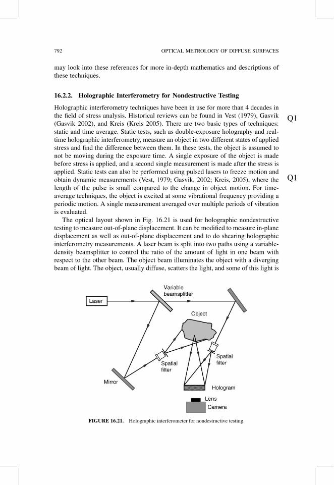
The optical layout shown in Fig. 16.21 is used for holographic nondestructive

testing to measure out-of-plane displacement. It can be modified to measure in-plane

displacement as well as out-of-plane displacement and to do shearing holographic

interferometry measurements. A laser beam is split into two paths using a variable-

density beamsplitter to control the ratio of the amount of light in one beam with

respect to the other beam. The object beam illuminates the object with a diverging

beam of light. The object, usually diffuse, scatters the light, and some of this light is

FIGURE 16.21. Holographic interferometer for nondestructive testing.

Q1

Q1


incident upon the hologram plane. The other beam is a reference beam directly

incident upon the hologram plane. The angle between the object beam and the

reference beam at the hologram plane will determine the spacing of the interference

fringes in the hologram. Because the hologram is simply the interference of two

beams of light, the difference between the path lengths of the object and reference

beams must be within the coherence length of the laser being used. If an argon-ion

laser with an etalon or a single-mode helium–neon laser is used, a coherence length

of many meters is attainable; whereas, if a multi-mode helium–neon laser is used, the

path lengths must be within a few centimeters of one another. To make an efficient

hologram, the reference beam should be 6–8 times brighter than the object beam at

the hologram plane, the polarizations of the two beams should be in the plane of

incidence, and the angle between the object and reference beams needs to be small

enough to produce resolvable interference fringes in the recording material.

Holographic interferometry techniques can be used to measure thermal changes in

optical elements, changes in optical surface shape due to mounting, changes in

deformable mirror shapes, and to study vibrational modes of optical elements,

mounts, or entire optical systems. These techniques can be used with diffuse

(ground) surfaces, specularly reflecting surfaces, and transmissive optical compo-

nents. One particular application of holographic nondestructive testing is to deter-

mine the mechanical and thermal properties of large unworked mirror blanks before

any time and money are spent to put optical surfaces on the blanks (Van Deelen and

Nisenson 1969). Both qualitative fringe data and quantitative displacement data may

be obtained.

Static Holographic Interferometry. For a static holographic measurement of an

object, a hologram of the object is made while the object is in one stress state. In order

for static measurements to work, the object must not move while the hologram is

being made. After the object stress state is changed, either a second hologram is

exposed as in double-exposure holographic interferometry, or the object is observed

through the hologram as in real-time holographic interferometry. In both cases, there

is a secondary interference between the wavefront generated before the change in

applied stress and the wavefront generated after the change in applied stress. For

double-exposure holography, both wavefronts are stored in the hologram. When the

hologram is illuminated with the reference wavefront, both wavefronts are recon-

structed. When these wavefronts are viewed through the hologram, cosinusoidal

secondary interference fringes are visible. The secondary interference fringes corre-

spond directly to the amount of object displacement between the two exposures. If

there is no change in the object between exposures, a single interference fringe will

be produced. Each fringe in the secondary interference pattern indicates one wave of

displacement along a direction bisecting the illumination and viewing directions of

the object.

For real-time holographic interferometry, one of the two wavefronts is stored in

the hologram, and the other wavefront is produced live by the test object. Once the

hologram is made and developed, care must be made to ensure that the hologram is

replaced in the same location so that the wavefront stored in the hologram can be

Q1


interfered with the live wavefront. Real-time holographic interferometry is very

similar to the use of the holographic test plate. Fringe location, fringe shape, and

test sensitivity are the same for real-time techniques as they are with double-exposure

techniques. If the object is in motion, static techniques can be used to provide

cosinusoidal fringes as long as a pulsed laser or high-speed shutter is used to freeze

the motion. The exposure time must be short enough that the object does not

move during it.

Figure 16.22 shows the recording geometry indicating the object displacement

vector L, and the sensitivity vector K. The sensitivity vector is defined as the

direction along which the object displacement is measured. The direction of the

sensitivity vector can vary across the object surface if the field of view is large, and if

the source illuminating the object and the viewing position are not located at infinity.

Mathematically, the secondary interference fringes for a static holographic measure-

ment at a single point in the viewing plane can be written as

I ¼ I0ð1 þ g cos�fÞ ð16:36Þ

where I0 is the dc intensity, g is the fringe visibility, and �f is the phase of the

secondary interference fringes corresponding to the difference (displacement)

between the two object states. The phase difference can be written as

�f ¼ K � L ð16:37Þ

The displacement of the object at a point x,y in the direction of the sensitivity vector

is given by

Dðx; yÞ ¼ �fðx; yÞl4p cosðc=2Þ ð16:38Þ

FIGURE 16.22. Recording geometry showing sensitivity vector and displacement vector.


where l is the illumination wavelength and c is the angle between the illumination

and viewing directions. The displacement measurement is usually a combination of

in-plane (along the surface of object) and out-of-plane (perpendicular to the object

surface) displacement. Specific setups can be made to measure only one of these

components. If all three components of displacement (x,y, and z) are desired, three

measurements must be made (Pryputniewicz and Stetson, 1976; Stetson, 1979, 1990;

Nakadate et al., 1981; Kakunai et al., 1985; Hariharan et al., 1987). As long as the

change in the object shape is small, the secondary interference fringes will be

localized at the object. If the applied stress causes the object to move (rigid-body

translation or rotation) as well as deform, the secondary interference fringes may not

be localized at the object (Vest, 1979; Hariharan, 1984).

An example showing the use of static holographic interferometry to test a

coupling flange from a helicopter is shown in Figure 16.23. This part was stressed

between exposures by applying a static force between the rim and the center of the

part.

In addition to displacement measurement and stress analysis, real-time or double-

exposure holographic interferometry can be used to contour objects with two

wavelengths, two indices of refraction, or two different angles of object illumination

(Hariharan, 1984).

Time-Average Holographic Interferometry. If the object is excited in a periodic

motion, a measurement can be made using a single exposure which averages over

many vibrational periods creating a time-average hologram (Powell and Stetson,

FIGURE 16.23. Double-exposure holographic interferometry fringes of helicopter coupling flange.

(Courtesy K. A. Stetson, United Technologies Research Center.)

Q1

Q1

Q1


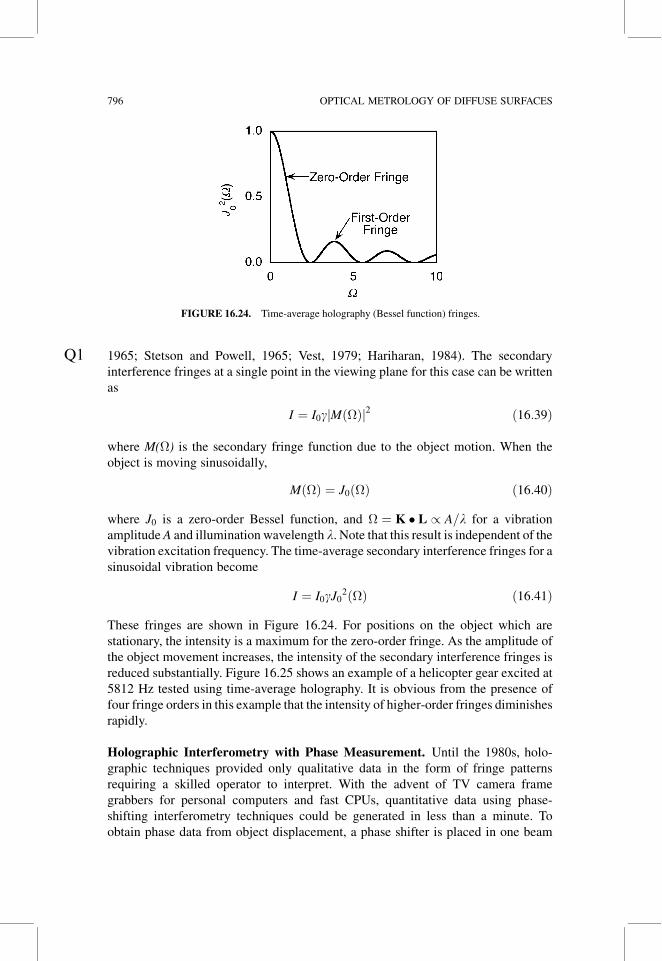
1965; Stetson and Powell, 1965; Vest, 1979; Hariharan, 1984). The secondary

interference fringes at a single point in the viewing plane for this case can be written

as

I ¼ I0gjMð�Þj2 ð16:39Þ

where M(�) is the secondary fringe function due to the object motion. When the

object is moving sinusoidally,

Mð�Þ ¼ J0ð�Þ ð16:40Þ

where J0 is a zero-order Bessel function, and � ¼ K � L / A=l for a vibration

amplitude A and illumination wavelength l. Note that this result is independent of the

vibration excitation frequency. The time-average secondary interference fringes for a

sinusoidal vibration become

I ¼ I0gJ02ð�Þ ð16:41Þ

These fringes are shown in Figure 16.24. For positions on the object which are

stationary, the intensity is a maximum for the zero-order fringe. As the amplitude of

the object movement increases, the intensity of the secondary interference fringes is

reduced substantially. Figure 16.25 shows an example of a helicopter gear excited at

5812 Hz tested using time-average holography. It is obvious from the presence of

four fringe orders in this example that the intensity of higher-order fringes diminishes

rapidly.

Holographic Interferometry with Phase Measurement. Until the 1980s, holo-

graphic techniques provided only qualitative data in the form of fringe patterns

requiring a skilled operator to interpret. With the advent of TV camera frame

grabbers for personal computers and fast CPUs, quantitative data using phase-

shifting interferometry techniques could be generated in less than a minute. To

obtain phase data from object displacement, a phase shifter is placed in one beam

FIGURE 16.24. Time-average holography (Bessel function) fringes.

Q1


of the interferometer shown in Figure 16.21. Standard phase-shifting techniques (as

described in Chapter 14) can be used with holographic interferometry techniques

which produce cosinusoidal fringes to generate a phase map of �f(x,y) correspond-

ing to the object displacement D(x,y) (Hariharan, 1984, 1985; Gasvik, 2002; Kreis,

2005).

An example of a phase measurement of out-of-plane displacement using real-time

holographic interferometry to measure changes due to mechanical stress is shown in

Figure 16.26. A hologram was made of a metal plate bolted on all four corners, and

the phase measurement was performed after tightening a screw pushing on the back

of the plate. The contour interval for Figure 16.26(a) is 0.3653 mm, and the angle

between the illumination and viewing directions is 60� yielding a peak-to-valley

displacement of 7.3 mm.

Quantitative data can also be extracted from time-average vibration fringes using

phase-shifting techniques (Neumann et al., 1970; Stetson, 1982; Oshida et al., 1983;

Nakadate and Saito, 1985; Stetson and Brohinsky, 1988). Three separate phase

measurements need to be taken (Stetson and Brohinsky, 1988). The first one is

made with the object vibrating and shifting the relative phase between the object and

reference beams as in standard phase-shifting interferometry. The second measure-

ment is made by applying a vibration of the same frequency as the object vibration to

a PZT in the reference beam of the interferometer. A bias phase between the object

and reference vibration is added such that the relative phase difference between the

vibrations is þp=3. Relative phase shifts between the object and reference beams are

then applied and standard phase-shifting methods are used to calculate the phase. A

third measurement is taken such that the relative phase difference between the object

and reference vibrations is �p=3. Assuming a sinusoidal object vibration and 90�

relative phase shifts for the phase calculations, one of the total of 12 frames of data

FIGURE16.25. Time-average holographic fringes of helicopter gear excited at 5812 Hz. (Courtesy K. A.

Stetson, United Technologies Research Center.)

Q1


recorded can be written as

Iji ¼ I0½1 þ g cosðfþ diÞJ0ð�þ bjÞ� ð16:42Þ

where di ¼ 0, p=2, p, and 3p/4, and bj ¼ �p=3; 0, and p/3. The amplitude of the

vibration can then be calculated using

� ¼ tan�1 1ffiffiffi3

p H1 � H3

2H2 � H1 � H3

� �� ð16:43Þ

where

H1 ¼ ðI11 � I13Þ2 þ ðI12 � I14Þ2 ¼ 4I20g

2J20ð�� p=3Þ ð16:44Þ

H2 ¼ ðI21 � I23Þ2 þ ðI22 � I24Þ2 ¼ 4I20g

2J20ð�Þ and ð16:45Þ

H3 ¼ ðI31 � I33Þ2 þ ðI32 � I34Þ2 ¼ 4I20g

2J20ð�þ p=3Þ ð16:46Þ

Eq. (16.43) assumes the form of cos2 for the fringes. Because of this, a look-up table

is necessary to find the difference between the J20ð�Þ and cos2ð�Þ functions

FIGURE 16.26. Out-of-plane displacement of a metal plate using phase-shifting interferometry techni-

ques with real-time holographic interferometry. (a) Two-dimensional contour plot with a contour interval of

0.3653 mm and (b) isometric contour plot. The angle between the illumination and viewing directions is 60�

yielding a peak-to-valley displacement of 7.3 mm.


(Stetson and Brohinsky, 1988). The error due to the difference between the J20ð�Þ and

cos2ð�Þ functions is dependent upon the fringe order, which can be determined from

the H2 measurement.

When the object under observation is not stable enough to capture consecutive

exposures with different phase shifts, phase information can be obtained from a

single interferogram using the Fourier-transform technique (Kreis, 1986, 1987) or

using a multiplexing scheme encoding all the phase information for multiple phase

shifts either onto multiple cameras (Koliopoulos, 1992) or onto a single camera

(North-Morris et al., 2005). For the Fourier transform technique, the Fourier Trans-

form of the fringe pattern is computed, one diffraction order is filtered out and then

shifted to zero frequency, and then this single order is inverse Fourier transformed to

obtain the phase distribution. This technique requires sinusoidal fringes and enough

straight ‘‘tilt’’ fringes to separate orders. When multiple phase shifts are encoded

within a single snapsnot, dynamic and random motion can be followed and tracked

quantitatively. These techniques are sensitive enough to be able to track thermal

microbreezes related to pulse and respiration cycles in humans (Creath and

Schwartz, 2005).

Digital Holographic Interferometry. In digital holographic interferometry, phase

and amplitude information are captured electronically. The intermediate hologram is

stored in digital memory and used to reconstruct the object after the second exposure

is made (Yaroslavsky, 2004; Kreis, 2005; Schnars and Jueptner, 2005). All of the

processing is done numerically and because of this these systems are more flexible

and faster than using a separate holographic recording media. As megapixel cameras

and sensors have became more available these types of measurements have become

easier and easier. More about this topic is discussed in the next section.

16.2.3. Speckle Interferometry and Digital Holography

The first digital holography techniques were based on speckle interferometry

(Dandliker, 2000; Joenathan and Tiziani, 2003). When TV cameras began being

used and digital images stored and processed in hardware via electronics, these

techniques were first named ‘‘electronic speckle pattern interferometry’’ (ESPI) and

often called TV holography (Lokberg and Slettemoen, 1987; Jones and Wykes,

1983). Because of the low spatial frequency response of TV cameras these techni-

ques measured in-line holograms (Gabor type holograms). The next step was to get

quantitative information by applying phase shifting methods utilizing a computer

with these ESPI techniques. These were called either ‘‘digital speckle pattern

interferometry’’ or ‘‘phase shifting speckle interferometry’’ (Nakadate and Saito,

1985; Creath, 1985b, 1986c; Robinson and Williams, 1986). As cameras with higher

spatial resolutions became available it became possible to make the off-axis holo-

grams that we are more familiar with. These techniques became know as digital

holography (Kreis, 2005; Schnars and Jueptner, 2005) or phase shifting ESPI

(Jacquot and Fournier, 2000; Gasvik, 2002). When encountering these techniques

Q1

Q1

Q1

Q1

Q1


in the literature there is not a common name, yet they are all based upon the same

principles. Nowadays the term digital holography refers to any type of hologram

stored and reconstructed digitally, and the term speckle interferometry also refers to

the same systems where it is obvious that speckle is present. The mechanisms for

creating interference are similar in both, and results are as well. What differentiates

one technique from another is how well different spatial frequency structures are

reconstructed, and how immune to noise the techniques are. Keep this in mind

through the rest of this chapter where speckle interferometry and digital holography

techniques are discussed.

Basics of Speckle Interferometry. When a laser beam is scattered off of a diffuse

surface, the scattered light has a grainy appearance. The grains are an interference

phenomenon known as speckle. The statistics of the speckle distribution depend upon

the statistics of the object surface. If imaged by a lens, the speckle are said to be

subjective, and the smallest speckle in the image will have a size equal to the Airy

disk 2.44 l/F# generated by the optical system, where F# is the working F-number of

the system (Goodman, 1975a). The intensity distribution and the statistics of the

speckle pattern are an indication of the roughness of the surface used to generate the

speckle pattern (Goodman, 1975a,b; Erf, 1978; Fujii and Lit, 1978). A speckle

pattern generated by an object surface can be thought of as the object’s fingerprint.

When the object is perturbed in some way, the speckle pattern will change in a

predictable way. Two different types of techniques are speckle photography and

speckle interferometry (Ennos, 1975; Stetson, 1975b; Pryputniewicz, 1985; Huntley,

1989). Both techniques involve the comparison of two or more speckle patterns. A

recently published book by Goodman (2006) reviews the uses and properties of

speckle.

Speckle interferometry usually includes a reference beam to enable measurement

of the phase change in the speckles. In speckle interferometry, it is assumed that the

speckles from one speckle pattern to another are correlated so that they do not shift by

more than the diameter of a speckle between exposures. Speckle photography looks

at the correlation between two speckle patterns where the fringes arise from a

translation between exposures and can be used to measure larger displacements.

The speckles from a small area of the two speckle patterns (translated with respect to

one another) generate Young’s fringes in the Fourier plane. For the rest of this

discussion we are going to concentrate upon speckle interferometry techniques

utilizing a reference beam.

To aid in understanding how speckle interferometry works, consider a diffuse

object placed in the object beam of a Twyman–Green interferometer and a photo-

graphic plate placed at the image of the object with an F# large enough to produce

visible speckle. After the speckle pattern is recorded and the photographic plate

replaced in the original position, no light will get through the negative plate because

the speckles line up with those stored in the photographic plate. This is similar to a

single fringe using the holographic test plate. As the object is tilted, fringes will be

seen which correspond to the tilt of the object. These fringes are modulated by a

speckle pattern, and appear noisy. The secondary interference fringes are also known

Q1

Q1

Q1

Q1


as speckle correlation fringes because they correspond to the correlation between the

speckles in the two fringe patterns (Jones and Wykes, 1983; Løkberg and Slettemoen,

1987). For speckle interferometry, the speckles are usually resolved by the recording

system; however, this is not a necessary condition (Creath, 1985a).

Speckle interferometry techniques can be used for the same applications as

holographic interferometry techniques (Dandliker, 2000; Jacquot and Fournier,

2000; Gasvik, 2002; Gastinger et al., 2003; Joenathan and Tiziani, 2003). Using a

single illumination wavelength, static and dynamic measurements of object displa-

cement provide the same results as holographic nondestructive testing. Just as in

holographic interferometry, the speckle interferometry nondestructive testing tech-

niques can measure only a single component of object displacement. This compo-

nent, in the direction of the sensitivity vector, is described in the section on

holographic interferometry for nondestructive testing. Two-wavelength techniques

can also be used to perform a reduced-sensitivity test equivalent to two-wavelength

holography or interferometry.

An in-line speckle interferometry setup for the measurement of out-of-plane

displacement is shown in Figure 16.27. The optical system is similar to those

described for holographic test techniques where the path lengths must be adjusted

to be within the coherence length of the source, the polarizations of the two beams

must be such that they are in the plane of incidence at the viewing plane, and the

speckle should be recorded in a plane conjugate to the test surface so that the

interference corresponds directly to changes in the object surface. Speckle inter-

ferometry techniques also utilize a small aperture which determines the size of the

speckle at the recording plane.

Essentially, speckle interferometry techniques perform the holographic interfero-

metry techniques described earlier without the need to make an intermediate

FIGURE 16.27. Speckle interferometry setup similar to that for making an in-line hologram.

Q1


hologram. The basic digital speckle interferometry technique was coined electronic

speckle-pattern interferometry (ESPI) (Archbold et al., 1970; Butters and Leendertz,

1971; Macovski et al., 1971; Biedermann and Ek, 1975; Ennos, 1975; Jones and

Wykes, 1983; Løkberg and Slettemoen, 1987). This technique originqally used a TV

camera as the recording device and processed interferograms in either electronics or

a computer or array processor. It was often sometimes called TV holography and now

is more often simply called digital holography. A slightly different variation on ESPI

which provides improved fringe contrast has been coined electro-optic holography

(EOH) by Stetson and Brohinsky (Stetson and Brohinsky, 1985, 1986, 1987;

Bushman, 1989; Feit, 1989; Stetson, 1989; Stetson et al., 1989). Phase measurements

can be applied to ESPI, DH and EOH to provide quantitative displacement maps of

the same data obtained in holographic interferometry.

Electronic Speckle-Pattern Interferometry. ESPI uses an optical setup similar to

that of Figure 16.27, where a TV camera, CCD camera, or detector array is placed at

the image of the test surface (Archbold et al., 1970; Butters and Leendertz, 1971;

Macovski et al., 1971; Biedermann and Ek, 1975; Ennos, 1975; Jones and Wykes,

1983; Løkberg and Slettemoen, 1987). Historically all of the processing was per-

formed in electronic hardware and results were displayed in real-time on a TV

monitor. Because standard video signals were generated, the results of a test could be

stored electronically for later viewing and processing.

For ESPI the limiting aperture size is adjusted so that the speckle will be resolved

by the camera. (When the speckles are reduced in size, the effect is to reduce the

contrast of the secondary interference fringes.) With static ESPI measurements, a

speckle interferogram of the object is recorded by the camera and stored electro-

nically. A single interferogram can be written as

I ¼ I0ð1 þ g cosfÞ ð16:47Þ

where I0 is the dc intensity, g is the visibility, and f is the phase of the interference

between the reference beam and the speckle pattern scattered by the object. After the

stress applied to the object is changed, Eq. (16.47) becomes

I ¼ I0ð1 þ g cosf0Þ ð16:48Þ

where f0 ¼ fþ�f, and �f is the phase change. The stored interferogram is then

subtracted from exposures recorded after a change in applied stress to the object, and

the difference is squared to yield

I2 ¼ 4I20g

2ðsin2 fÞ½sin2ð�f=2Þ� ð16:49Þ

This equation shows that there are fringes due to object displacement �f as well as

fringes due to the phase of speckles f resulting from the interference between the

reference and speckled object beams. The sin2f term causes modulation of the

speckle and makes the fringes noticeably noisy. Much of the research effort in the last

Q1

Q1

Q1


two decades has been to reduce this noise due the inherent properties of the speckle

(see for example (Federico et al., 2000; Kolenovic et al., 2003)). That which is the

signal is also a noise source depending upon your point of view (Creath, 1993).

Time-average measurements can be made with ESPI using a single frame of data.

For a vibrating object, the signal at the camera for a single detector point averaged

over many cycles of vibration is given by

I ¼ I0½1 þ g cosðfÞMð�Þ� ð16:50Þ

where f is the phase difference between the object and reference beams, and � is

proportional to the amplitude of the object displacement. In order to process this

signal, the dc component is filtered out, and then the signal is rectified and squared to

yield

I ¼ I0gðcos2 fÞjMð�Þj2 ð16:51Þ

Note that this expression has a factor of cos f, which is not included in the time-

average holographic vibration fringes given by Eq. (16.39). The cos2f term is due to

the phase of the speckles, and causes the secondary fringes to be noisy. For a

sinusoidal object motion, Eq. (16.51) can be rewritten as

I ¼ I0gðcos2 fÞJ20ð�Þ ð16:52Þ

Because the processing for static and dynamic measurements is performed in

electronics, fringe data can be obtained with ESPI at video frame rates (25 or

30 frames per second) or faster depending upon the camera and data acquisition

hardware. This speed enables measurements to be made even when the object is not

very stable. This same math also can be used to describe time-average digital

holography.

Example of fringes obtained using ESPI are shown in Figures 16.28 and 16.29.

Fringes for a single frame of time-average data for a vibrating flat plate are shown in

Figure 16.28(a). By averaging a number of statistically independent fringe patterns

obtained by changing the angle of illumination on the object, the speckle noise in the

fringe pattern can be reduced as shown in Figure 16.28(b) (Creath, 1985c).

Figure 16.29 shows a time-average interferogram of a car body vibrating at

110 Hz (Malmo and Vikhagen, 1988). These data were taken with the car sitting

in a parking lot. The body was covered with retroreflective tape and excited using a

loud speaker on the seat. A commercially-available ESPI instrument with a 7 mW

helium–neon laser was used for the measurements.

Electrooptic Holography. A major disadvantage of ESPI is that after processing

the interference fringe data, there are terms proportional to the phase of the speckle

produced by the interference between the reference beam and the speckle in the

object beam. These terms cause noisy-looking fringes. By processing the data

differently, Stetson and Brohinsky have shown that the speckle term can be removed

Q1

Q1


(Stetson and Brohinsky, 1985, 1986, 1987; Bushman, 1989; Feit, 1989; Stetson,

1989; Stetson et al., 1989). The electro-optic holography (EOH) system uses the

same optical setup as ESPI; however, one mirror in the reference beam is mounted on

a piezo-electric translator (PZT) to provide relative phase shifts between the object

and reference beams. Data can be taken at TV frame rates and stored on videotape.

The major difference of EOH from ESPI is the use of a pipeline image processor to

handle a large number of images at once instead of the simple electronics of ESPI

which process a single frame at a time.

For static measurements, this technique utilizes four frames of data with 90�

relative phase shifts between the object and reference which are stored in an array

processor. One of these frames of data is written as

Ii ¼ I0½1 þ g cosðfþ diÞ� ð16:53Þ

FIGURE16.28. ESPI interferogram of vibration mode of a flat plate using (a) single interferogram and (b)

with speckle averaging. (From Creath, 1985c.)

FIGURE 16.29. ESPI interferogram of car body vibrating at 110 Hz taken in parking lot. (From Malmo

and Vikhagen, 1988.)

Q5

Q1


where di ¼ 0, p/2, p, and 3p/4 are the applied phase shifts for I1, I2, I3, and I4. After

the applied stress on the object is changed, four more frames of data are recorded

with 90� relative phase shifts:

I0i ¼ I0½1 þ g cosðf0 þ diÞ� ð16:54Þ

where f0 ¼ fþ�f. The eight frames of data are combined in a pipeline image

processing system to yield

I ¼ffiffiffiffiffiffiffiffiffiffiffiffiffiffiffiffiffiffiffiffiffiffiffiffiffiffiffiffiffiffiffiffiffiffiffiffiffiffiffiffiffiffiffiffiffiffiffiffiffiffiffiffiffiffiffiffiffiffiffiffiffiffiffiffiffiffiffiffiffiffiffiffiffiffiffiffiffiffiffiffiffiffiffiffiffiffiffiffiffiffiffiffiffi½ðI1 � I3Þ þ ðI01 � I03Þ�

2 þ ½ðI2 � I4Þ þ ðI02 � I04Þ�2

q

¼ 4I0g cosð�f=2Þð16:55Þ

This calculation produces fringes proportional to the phase change due to the object

displacement. There is no extra term due to the speckles. The calculation involves

only addition, subtraction, and the application of a look-up table to find the square

root of the sum of the squares of two numbers. This is easily accomplished using an

array processor. As the applied stress to the object changes, four new frames need to

be obtained. As long as the applied stress is slowly varying, the secondary inter-

ference fringes can be calculated after each video frame is recorded and 90� relative

phase shifts are applied between consecutive video frames. Thus, these fringes can be

calculated and displaced at TV frame rates using an image-processing system.

For a time-average measurement using EOH, four time-average frames of data are

taken while the object is vibrating with 90� relative phase shifts. One of these frames

is written as

Ii ¼ I0½1 þ g cosðfþ diÞMð�Þ� ð16:56Þ

where the phase shifts di are 0, p/2, p, and 3p/4. These four frames can then be

combined to obtain secondary fringes using

I ¼ffiffiffiffiffiffiffiffiffiffiffiffiffiffiffiffiffiffiffiffiffiffiffiffiffiffiffiffiffiffiffiffiffiffiffiffiffiffiffiffiffiffiffiðI1 � I3Þ2 þ ðI2 � I4Þ2

q¼ 2I0gjMð�Þj ð16:57Þ

which can be written as

I ¼ffiffiffiffiffiffiffiffiffiffiffiffiffiffiffiffiffiffiffiffiffiffiffiffiffiffiffiffiffiffiffiffiffiffiffiffiffiffiffiffiffiffiffiðI1 � I3Þ2 þ ðI2 � I4Þ2

q¼ 2I0gjJ0ð�Þj ð16:58Þ

for a sinusoidal object vibration. Note that the speckle modulation term is not present

with this technique.

An example of fringes produced with EOH is shown in Figure 16.30. Figure 16.30(a)

shows a rectangular plate undergoing static deflection and Figure 16.30(b) shows a time-

average vibration mode of the same plate. EOH can also be used for shearography

(shearing speckle interferometry) by utilizing a different optical system (Stetson, 1989).Q1


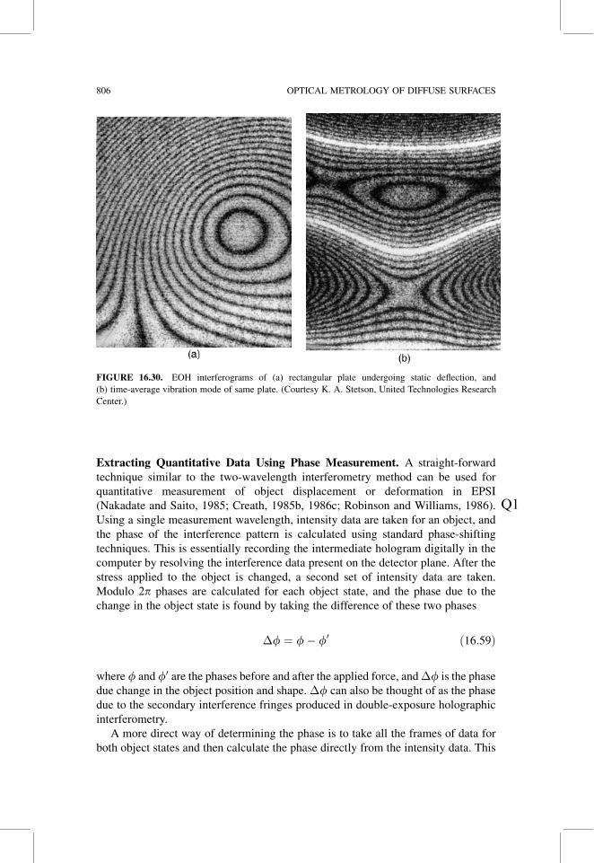
Extracting Quantitative Data Using Phase Measurement. A straight-forward

technique similar to the two-wavelength interferometry method can be used for

quantitative measurement of object displacement or deformation in EPSI

(Nakadate and Saito, 1985; Creath, 1985b, 1986c; Robinson and Williams, 1986).

Using a single measurement wavelength, intensity data are taken for an object, and

the phase of the interference pattern is calculated using standard phase-shifting

techniques. This is essentially recording the intermediate hologram digitally in the

computer by resolving the interference data present on the detector plane. After the

stress applied to the object is changed, a second set of intensity data are taken.

Modulo 2p phases are calculated for each object state, and the phase due to the

change in the object state is found by taking the difference of these two phases

�f ¼ f� f0 ð16:59Þ

where f and f0 are the phases before and after the applied force, and �f is the phase

due change in the object position and shape. �f can also be thought of as the phase

due to the secondary interference fringes produced in double-exposure holographic

interferometry.

A more direct way of determining the phase is to take all the frames of data for

both object states and then calculate the phase directly from the intensity data. This

FIGURE 16.30. EOH interferograms of (a) rectangular plate undergoing static deflection, and

(b) time-average vibration mode of same plate. (Courtesy K. A. Stetson, United Technologies Research

Center.)

Q1


can be written as

�f ¼ tan�1 sinð�fÞcosð�fÞ

� �¼ tan�1 sinðf� f0Þ

cosðf� f0Þ

� �¼ tan�1 sinf cosf0 � cosf sinf0

cosf cosf0 þ sinf sinf0

� �

ð16:60Þ

which for the four-frame method becomes

�f ¼ tan�1 ðI4 � I2ÞðI01 � I03Þ � ðI1 � I3ÞðI04 � I02ÞðI1 � I3ÞðI01 � I03Þ þ ðI4 � I2ÞðI04 � I02Þ

� �ð16:61Þ

where Ii and Ii0 are the ith data frames taken for each object state. This process will

work for any phase measuring algorithm where the phase fi can be written in terms

of a numerator function Ni and a denominator function Di as

fi ¼ tan�1 sinfi

cosfi

� �¼ tan�1 Ni

Di

� �ð16:62Þ

The phase of the difference between measurement 1 and measurement 2 is then

given by

�f ¼ tan�1 sinðf1 � f2Þcosðf1 � f2Þ

� �¼ tan�1 N1D2 � D1N2

D1D2 þ N1N2

� �ð16:63Þ

Another type of phase calculation requires data at only two different phase shifts

for displacement/deformation measurement. A total of four frames of data, two

before and two after are all the data required in a method developed by Kerr et al.

(1990).

Another variation utilizes EOH. The eight frames of data taken for a static

measurement [Eqs. (16.53) and (16.54)] can be used to calculate the phase change

�f due to the displacement of the object,

�f ¼ tan�1 C3 � C4

C1 � C2

� �ð16:64Þ

where the quantities Ci are given by

C1 ¼ ½ðI1 � I3Þ þ ðI01 � I03Þ�2 þ ½ðI2 � I4Þ þ ðI02 � I04Þ�

2 ð16:65ÞC2 ¼ ½ðI1 � I3Þ � ðI01 � I03Þ�

2 þ ½ðI2 � I4Þ � ðI02 � I04Þ�2 ð16:66Þ

C3 ¼ ½ðI1 � I3Þ þ ðI02 � I04Þ�2 � ½ðI2 � I4Þ þ ðI01 � I03Þ�

2 ð16:67ÞC4 ¼ ½ðI1 � I3Þ � ðI02 � I04Þ�

2 � ½ðI2 � I4Þ � ðI01 � I03Þ�2 ð16:68Þ

Q1


These calculations only involve simple calculations and the use of lookup tables

which can be done in an array processor. The modulo 2p phase corresponding to the

object displacement can be calculated in real time at video frame rates. Quantitative

measurements of time-average interferograms can be made using the techniques

described for holographic nondestructive testing in section 16.2.2.3 and Eqs. (16.42)

thru (16.46) (Pryputniewicz and Stetson, 1989).

In practice there are numerous other ways that have been developed to extract

phase information for speckle interferometry and holographic interferometry. Most

of the algorithms are tailored to a specific application and a specific type of

measurement and optical system.

Dynamic Techniques. In the real world of testing diffuse objects using speckle

interferometry and digital holography, it can be difficult to ensure that an object is

stable and not moving relative to the instrument. It is desirable to have instrumenta-

tion that is either insensitive to vibration or can freeze motion to make measurements.

For this, many different techniques have been developed to cope with these situa-

tions. This essentially enables taking data of arbitrarily moving objects and being

able to track motion, modes of vibration, flows, and even watch shock waves travel.

For dynamic measurements, there are many different commercial systems available

that fit in a briefcase size or are mounted on a tripod. Most of the work published on

dynamic techniques in the past decade has originated in Europe and been initiated to

find solutions for automotive applications.

To freeze motion, some sort of pulsed laser is usually implemented. Pulsed lasers

can provide enough energy in a single pulse to get a decent exposure on the return

with a standard silicon detector array. Fast shutters can also be used, but then more

overall power is needed from the source to get a sufficient exposure unless low-light

level imaging systems are implemented. Any of the techniques mentioned so far in

this chapter can be implemented using a pulsed laser or fast shutter including all of

the quantitative techniques that determine phase. It is also possible to unwrap phase

in time as well as space to follow motion in time (Ruiz et al., 2003). Amplitude and

phase information can both be extracted and added to shape information to determine

complex motions and perform active metrology measurements (Osten, 2003). Mod-

ifications of the optical system utilizing endoscopes and fibers can enable getting

measurements in tight spaces of otherwise hidden surfaces (Pedrini et al., 2003) or

biological objects (Pedrini et al., 2005). These types of developments drastically

increase the possible applications and usefulness of digital holography and speckle

interferometry.

Shearography as described in the next subsection is one way to ensure that

vibrations and relative motions between the interferometer and object don’t hamper

the data. Another way to get quantitative data from a single fast snapshot is to use

phase measuring techniques that either require only a single interferogram such as

Fourier Transform techniques (Kreis, 1986, 1987) or those that multiplex phase data

using polarization techniques to take all necessary data at once (Koliopoulos, 1992)

(North-Morris et al., 2005).

Q1


Shearography. Just as there are many ways to test optical components with shearing

interferometry, so there are many ways to test diffuse surfaces with speckle shearing

interferometry also known as shearography (Joenathan and Tiziani, 2003; Steinchen

and Yang, 2003). Shearography tests a surface relative to itself. Because it is common

path, it is insensitive to vibrations and relative motion between the part under test and

the interferometer. But, like all shearing interferometers, it does not directly measure

displacement or shape. Instead it measures the slope of the displacement or shape in

the direction of the shear. It can be used with phase measurement techniques as

described earlier in this chapter to quantitatively extract the slope. To get to

displacement or shape from the slope data, the techniques are similar to those

described in the shearing interferometer chapter of this book. Steinchen and Yang

outline numerous techniques in their book Digital Shearography (Steinchen and

Yang, 2003).

Low Coherence Techniques. Low coherence techniques combine a longer depth-

resolved measurement range with speckle interferometry and digital holography

techniques (Gastinger et al., 2003; Martinez-Leon et al., 2004; Gastinger and

Winther, 2005). Like low coherence interferometry (also known as white light

interferometry, or vertical scanning interferometry) low coherence speckle techni-

ques follow the high coherence fringe and map out where the greatest fringe contrast

is. These techniques require scanning in depth in order to make up a composite phase

map and are similar to the interference microscope techniques described in Chapter

15 of this book.

REFERENCES

Amridror I., The Theory of the Moire Phenomenon. Kluwer Academic Publishers, Dordrecht,

2000.

Armitage D., I. Underwood et al., Microdisplays Move Outside the Box, OE magazine, 2002,

pp. 28–30.

Creath K., ‘‘Speckle: Signal or Noise?’’ Proceedings FRINGE 93 Bremen 1993, W. Jueptner

and W. Osten (Eds.), Akademie Verlag, Berlin, pp. 97–102.

Creath K. and G. E. Schwartz, ‘‘The Dynamics of Life: Imaging Temperature and Refractive

Index Variations Surrounding Material and Biological Systems with Dynamic Interfero-

metry’’, Fringe 2005: The 5th International Workshop on Automatic Processing of Fringe

Patterns. W. Osten (Eds.), Springer-Verlag, Berlin, 2005, pp. 588–596.

D’Apuzzo N., ‘‘Overview of 3D Surface Digitization Technologies in Europe,’’ Proc. SPIE

6056, 605605:1–13, (2006).

Dandliker R., ‘‘The Story of Speckles in Interferometry,’’ Interferometry in Speckle Light, P.

Jacquot and J.-M. Fournier (Eds.), Springer Verlag, Berlin,2000, pp. 3–10.

Federico A., G. H. Kaufmann et al., ‘‘Speckle Noise Reduction in ESPI Fringes Using Wavelet

Shrinkage,’’ Interferometry in Speckle Light, P. Jacquot and J.-M. Fournier (Eds.), Springer

Verlag, Berlin, 2000, pp. 397–404.

Q4

Q4

REFERENCES 809

Frankowski G., M. Chen et al., ‘‘Real-Time Shape Measurement With Digital Stripe Projection

by Texas Instruments Micromirror Devices DMDTM,’’ Proc. SPIE 3958, 90–105 (2000).

Gastinger K., O. J. Lokberg et al., Speckle Metrology 2003, SPIE Proc 4933, Bellingham, WA,

SPIE, 2003.

Gastinger K. and S. Winther, ‘‘Optimisation of Low Coherence Speckle Interferometry (LSCI)

for Characterisation of Multi-layered Materials,’’ Proc. SPIE 5858, 58580K:1-12 (2005).

Gastinger K., S. Winther et al., ‘‘Low-Coherence Speckle Interferometry (LCSI) for Char-

acterisation of Adhesion in Adhesive Bonded Joints,’’ Proc. SPIE 4933, 59–65 (2003).

Gasvik K. J., Optical Metrology, 3rd Ed., John Wiley and Sons, Chichester, England, (2002).

Harding K., ‘‘Latest Optical Methods for Industrial Dimensional Metrology,’’Proc. SPIE 6000,

600001:1–14 (2005).

Huang P. S. and S. Zhang, ‘‘3D Optical Measurement Using Phase Shifting Based Methods,’’

Proc. SPIE 6000, 600002:1–10 (2005).

Hung Y. Y., L. Lin et al., ‘‘Practical Three-Dimensional Computer Vision Technqiues for Full-

Field Surface Measurement,’’ Opt. Eng., 39 (1), 143–149 (2000).

Jacquot P. and J.-M. Fournier, Interferometry in Speckle Light: Theory and Applications,

Springer Verlag, Berlin, 2000.

Joenathan C. and H. J. Tiziani, ‘‘Speckle and Speckle Metrology,’’ TheOptics Encyclopedia, T.

G. Brown, K. Creath, H. Kogelnik (Eds.), Wiley-VCH, Berlin, 2003, pp. 2709–2773.

Kolenovic E., W. Osten et al., ‘‘Improvement of Interferometric Phase Measurements by

Consideration of the Speckle Field Topology,’’ Proc. SPIE 4933, 206–211 (2003).

Koliopoulos C. L., ‘‘Simultaneous Phase-shift Interferometer,’’ Advanced Optical Manufac-

turing and Testing II, vol. 1531, V. J. Doherty (Ed.), SPIE, Bellingham, WA, 1992, pp. 119–

127.

Koninckx T. P. and L. Van Gool, ‘‘Real-Time Acquisition by Adaptive Structured Light,’’ IEEE

Trans Pattern Analysis and Machine Intelligence, 28 (3), 432–445 (2006).

Kowarschik R., P. Kuhmstedt et al., ‘‘Adaptive Three-Dimensional Measurement with Struc-

tural Light,’’ Opt. Eng., 39, 150–158 (2006).

Kreis T., Handbook of Holographic Interferometry. Wiley-VCH, Weinheim, Germany, 2005.

Kujawinska M. and D. Malacara, ‘‘Optical Metrology of Diffuse Objects: Full-Field Methods’’

in: Handbook of Optical Engineering, D. Malacara (Ed.), Marcel Dekker Inc, New York,

2001, pp. 493–522.

Martinez-Leon L., G. Pedrini et al., ‘‘Short-Coherence Digital Holography for the Investigation

of 3D Microscopic Samples,’’ Proc. SPIE 5457, 528–537 (2004).

Mix P. E., Introduction to Nondestructive Testing: A Training Guide, Second Edition, John

Wiley and Sons, Hoboken, NJ, 2005.

North-Morris M., J. Millerd et al., ‘‘Dynamic Phase-Shifting Electronic Speckle Pattern

Interferometer,’’ Proc SPIE 5869, 58691B:1–9 (2005).

Notni G., S. Riehemann et al., ‘‘OLED Microdisplays – A New Key Element for Fringe

Projection Setups,’’ Proc. SPIE 5532, 170–177 (2004).

Osten W., ‘‘Active Metrology by Digital Holography,’’ Proc. SPIE 4933, 96–110 (2003).

Patorski K. and M. Kujawinska, Handbook of the Moire Fringe Technique, Elsevier Science

Publishers, Amsterdam, 1993.

Pedrini G., I. Alexeenko et al., ‘‘Pulsed Endoscopic Digital Holographic Interferometry for

Investigation of Hidden Surfaces,’’ Proc. SPIE 4933, 123–128 (2003).

Q4

Q4

Q4

Q4

Q4

Q4

Q4

Q4


Pedrini G., I. Alexeenko et al., ‘‘Digital Holographic Interferometry for Investigations in

Biomechanics,’’ Proc. SPIE 5776, 325–332 (2005).

Post D., B. Han et al., High Sensitivity Moire: Experimental Analysis for Mechanics and

Materials, Springer, 1997.

Proll K.-P., J.-M. Nivet et al., ‘‘Application of Liquid Crystal Spatial Light Modulator for

Brightness Adaptation in Microscopic Topometry,’’ Applied Optics 39, 6430–6435 (2003).

Reich C., R. Ritter et al., ‘‘3D Shape Measurement of Complex Objects by Combining

Photogrammetry and Fringe Projection,’’ Optical Eng. 39 (1), 224–231 (2000).

Ritter R. and R. Hahn, ‘‘Contribution to Analysis of the Reflection Grating Method,’’ Optics

Lasers Eng. 4 (1), 13–24 (1983).

Ruiz P. D., J. M. Huntley et al., ‘‘Recent Advances in Temporal Phase-Shifting Speckle

Interferometry,’’ Proc. SPIE, 4933, 297–304 (2003).

Salvi J., J. Pages et al., ‘‘Pattern Codification Strategies in Structured Light Systems,’’ Pattern

Recognition 37, 827–849 (2004).

Schnars U. and W. Jueptner, Digital Holography: Digital Hologram Recording, Numerical

Reconstruction, and Related Techniques, Springer Verlag, Berlin, 2005.

Steinchen W. and L. Yang, Digital Shearography: Theory and Application of Digital Speckle

Pattern Shearing Interferometry, SPIE, Bellingham, WA, 2003.

Walker C. A. (Ed.), The Practical Application of the Moire Fringe Method in the Measurement

of Strain and Shape, IOP Publishing, Bristol, UK, 2004.

Wyant J. C., 2006, Moire Patterns. http://www.optics.arizona.edu/jcwyant/MoirePatterns/

MoirePatterns.htm.

Yaroslavsky L., Digital Holography and Digital Image Processing: Principles, Methods,

Algorithms, Kluwer Academic Publishers, Boston, 2004.

Q4

Q4

Q4

Q4

Q4

REFERENCES 811

Author Query

Q1. Please check the unlinked references, which are not cited in the ref. list.

Q2. Please check whether the figure is correct or not.

Q3. Please provide the old reference list.

Q4. Please provide the list of author.

Q5. Please check the change made.

16 - University of Arizonakcreath/pdf/pubs/2007_KC_JS_JC… · · 2010-03-0316.1. MOIRE´ AND...

Documents

Transcript of 16 - University of Arizonakcreath/pdf/pubs/2007_KC_JS_JC… · · 2010-03-0316.1. MOIRE´ AND...