1'6 )25 '(6,*1 - taekemdejong.nl WIND WATER/SUN blz 8 … · Prof.dr.ir. T. M. de Jong ed....

COLOFON

Authors: Taeke M. de Jong (ed.) Riet M.J. Moens-Gigengack Cees van den Akker Clemens M. Steenbergen

Production: Marlies Wenmeekers-Thomas

Publication and distribution by: 2004, Publicatiebureau Bouwkunde Delft University of Technology, Faculty of Architecture P.O. Box 5043 2600 GA Delft The Netherlands Telephone: +31 15 27 84737 Telefax: +31 15 27 83030

Copyright ©: The authors

Cover design: Thomas-Luuk Borest

Inspirit by the project Flagstaff: Roden Crater, by artist James Turrell, Arizona Sources:

James Turrell: The Other Horizon; by Peter Noever, Daniel Birnbaum, Georges Didi-Hubermann, James Turrell (book)

Baumeister 8/01; p. 43-48

Architecture and Urbanism 02:07; nr 382

URL source: http://www.rodencrater.org

3

Sun wind water earth life and living; legends for design

Prof.dr.ir. T. M. de Jong ed. 2004-03-15 Drs. M.J. Moens Prof.dr.ir. C. van den Akker Prof.dr.ir. C.M. Steenbergen

BkM1U01 territory BkVk11 sun wind water

www.bk.tudelft.nl/urbanism/team publications 2003

5

Contents 1 SUN ....................................................................................................... 81.1 ENERGY...........................................................................................................................................91.2 SUN...............................................................................................................................................241.3 TEMPERATURE ...............................................................................................................................371.4 PLANTING (PROF.DR.IR.C.M. STEENBERGEN; DRS. M.J. MOENS)......................................................52

2 WIND ................................................................................................... 902.1 GLOBAL ATMOSPHERE.....................................................................................................................912.2 NATIONAL CHOICE OF LOCATION.......................................................................................................962.3 REGIONAL CHOICE OF LOCATION ....................................................................................................1052.4 LOCAL MEASURES .........................................................................................................................1112.5 DISTRICT AND NEIGHBOURHOOD VARIANTS......................................................................................1242.6 ALLOTMENT OF HECTARES.............................................................................................................1332.7 SOUND AND NOISE ........................................................................................................................138

3 WATER (PROF.DR.IR. C. VAN DEN AKKER)............................................ 1473.1 WATER BALANCE ..........................................................................................................................1483.2 RIVER DRAINAGE...........................................................................................................................1523.3 WATER RESERVOIRS .....................................................................................................................1673.4 POLDERS .....................................................................................................................................1753.5 NETWORKS AND CROSSINGS..........................................................................................................189

4 EARTH (DRS. M.J. MOENS) ................................................................. 1994.1 KILOMETRES: GEOMORPHOLOGICAL LANDSCAPES ...........................................................................2014.2 METRES: SOIL UNITS .....................................................................................................................2204.3 MILLIMETRES: SOIL STRUCTURE .....................................................................................................2374.4 MICROMETRES: PHYSICAL-CHEMICAL COMPOSITION.........................................................................2434.5 SOIL POLLUTION............................................................................................................................2464.6 SITE PREPARATION .......................................................................................................................2644.7 CABLES AND PIPES........................................................................................................................2884.8 MAP ANALYSIS ..............................................................................................................................312

5 LIFE ................................................................................................... 3165.1 DIVERSITY, SCALE AND DISPERSION................................................................................................3175.2 ECOLOGIES ..................................................................................................................................3255.3 LEGENDS BY SCALE.......................................................................................................................3475.4 NATURAL HISTORY........................................................................................................................3655.5 VALUING NATURE .........................................................................................................................3775.6 MANAGING NATURE ......................................................................................................................394

6 HUMAN LIVING .................................................................................... 4086.1 ADAPTATION AND ACCOMMODATION...............................................................................................4096.2 THE HISTORY OF DUTCH HABITAT...................................................................................................4346.3 RECENT FIGURES..........................................................................................................................4516.4 DENSITIES....................................................................................................................................475

7 ENVIRONMENT .................................................................................... 4957.1 DEFINITION...................................................................................................................................4977.2 ENVIRONMENTAL PROBLEMS..........................................................................................................4997.3 ENVIRONMENTAL HYGIENE.............................................................................................................5027.4 TRANSMISSION .............................................................................................................................5097.5 IMMISSION AND EXPOSITION ...........................................................................................................5177.6 CREATING NORMS.........................................................................................................................5217.7 ENVIRONMENTAL CRITERIA FOR EVALUATION...................................................................................5267.8 ENVIRONMENTAL GAINS AND LOSSES DUE TO BUILDING ....................................................................533

6

8 LEGENDS FOR DESIGN ......................................................................... 5498.1 RESOLUTION AND TOLERANCE .......................................................................................................5508.2 SCALE-SENSITIVITY .......................................................................................................................5518.3 UNCONVENTIONAL TRUE SCALE LEGEND UNITS ................................................................................5528.4 REFERENCES ON LEGENDS FOR DESIGN .........................................................................................5558.5 COMPOSITION ANALYSIS ................................................................................................................5568.6 THE SCALE LEVEL AT WHICH ONE SEPARATES AND MIXES..................................................................5658.7 LEGENDS FOR DESIGN ...................................................................................................................5888.8 BOUNDARIES OF IMAGINATION........................................................................................................593

ENCLOSURES ......................................................................................... 606ENCLOSURE 1 THE TAXONOMY OF DUTCH PLANT FAMILIES......................................................................607ENCLOSURE 2 RANGORDENING VAN VESTIGINGEN NAAR OMSTREEKS 2000 IN NEDERLAND AANWEZIG

‘DRAAGVLAK’ PER VESTIGING IN INWONERS .....................................................................................611ENCLOSURE 3 TABLES TOKEN FROM THE STATISTICAL YEARBOOK 2001 ..................................................618ENCLOSURE 4 VNG TABLE 1; BUSINESS TYPES AND THEIR ENVIRONMENTAL IMPACT EXPRESSED IN METRES622ENCLOSURE 5 VNG TABLE 2 INSTALLATION TYPES AND THEIR ENVIRONMENTAL IMPACT EXPRESSED IN

METRES........................................................................................................................................636

KEY WORDS ........................................................................................... 639

QUESTIONS ............................................................................................ 664

7

Motivation Sun, wind, water, earth and life touch our living senses immediately, always, everywhere and without any intervention of reason. They simply are there in their unmatched variety, moving us, our moods, memories, imaginations, intentions and plans.

However, the designer transforming sun into light, air into space and water into life touches pure mathematics next to senses. Mathematicians left alone destroy mathematics releasing it from senses, losing their unmatched beauty and relief, losing their sense for design. To restore that intimate relation, the most freeing part of our European cultural heritage my great examples are Feynman’s lectures on physics, D’Arcy Thomson’s ‘On Growth and Form’ and Minnaert’s ‘Natuurkunde van het vrije veld’ (‘Outdoor physics’). Minnaert elaborated the missing step from feeling to estimating. I am sitting in the sun. How much energy do I receive, how much I send back into universe? I am walking in wind. How much pressure do I receive and how much power my muscles have to overcome? It is the same pressure giving form to the sand I walk on or giving form and movement to the birds above me! I am swimming in the oldest landscape of all ages, the sea. How can I survive?

No longer can I escape from reasoning, from looking for a formula, a behaviour that works. But this reasoning is next to senses and once I found a formula I can leave the reasoning behind going back into senses and sense. The formula takes its own path in my Excel sheet as a living thing. It ‘behaves’. Look! Does it take the same path as the sun, predicting my shadow? Put a pencil and a ruler in the sun. Measure, compare, lose or win your competition with the real sun as Copernicus did. Mathematics have no longer much to do with boring calculations. Nowadays computers do the work, we do the learning. They sharpen our reasoning and senses. We see larger contexts and smaller details then ever before discovering scale. Discovering telescopic and microscopic scale we find the multiple universe we live in, freeing us from boredom forever, producing images no human can invent. We do not believe our eyes and ears, we discover them. It challenges our imagination in strange worlds no holiday can equal. Life math is a survival journey with excitement and suspense.

But do we understand the sun? No, according to Kant (1976) we design a sun behaving like the sun we know from our position and scale of time and space we live in. We never know for sure whether it will behave tomorrow in the same way as our sheet does. But we have made something that works here and now.‘Yes! It works.’ That is designer’s joy.

Feynman, R. P., R. B. Leighton, et al. (1977,1963) The Feynman lectures on physics I (Menlo Park, California) Addison-Wesley Publishing Company ISBN 0-201-02010-6-H / 0-201-02116-1-P.

Feynman, R. P., R. B. Leighton, et al. (1977,1964) The Feynman lectures on physics II (Menlo Park, California) Addison-Wesley Publishing Company ISBN 0-201-02117-X-P / 0-201-02011-4-H.

Feynman, R. P., R. B. Leighton, et al. (1966,1965) The Feynman lectures on physics III (Menlo Park, California) Addison-Wesley Publishing Company ISBN 0-201-02118-X-P / 0-201-02114-9-H.

Kant, I. (1976) Kritik der reinen Vernunft (Frankfurt am Main) Suhrkamp Verlag. Minnaert, M. G. J. (1974) De natuurkunde van 't vrije veld. Deel I. Licht en kleur in het landschap

(Zutphen) Thieme & Cie ISBN 90-03-90780-3. Minnaert, M. G. J. (1975) De natuurkunde van 't vrije veld. Deel 2. Geluid, warmte, electriciteit

(Zutphen) Thieme & Cie ISBN 90-03-90790-0. Minnaert, M. G. J. (1971) De natuurkunde van 't vrije veld. Deel 3. Rust en beweging (Zutphen)

Thieme & Cie ISBN 90-03-90840-0. Minnaert, M. G. J. (1993) Light and color in the outdoors (New York, N.Y.,) Springer ISBN

0.387.94413.3 p; 0.387.97935.2; 3.540.97935.2. Thomson, D. A. W. (1961) On growth and form (Cambridge UK) Cambridge University Press ISBN 0

521 43776 8 paperback.

References are given on the end of every sub-chapter. Authors are included in the final key word list.

1 Sun 1.1 ENERGY...........................................................................................................................................9

1.1.1 Entropy .............................................................................................................................101.1.2 Energetic efficiency...........................................................................................................121.1.3 Global energy....................................................................................................................141.1.4 National energy.................................................................................................................171.1.5 Power supply ....................................................................................................................211.1.6 Local energy storage.........................................................................................................221.1.7 References to Energy .......................................................................................................23

1.2 SUN...............................................................................................................................................24

1.2.1 Looking from the universe ( and latitude ) .................................................................24

1.2.2 Looking from the Sun (culmination and declination ).....................................................251.2.3 Looking back from Earth (azimuth and sunheight) ............................................................261.2.4 Time on Earth ...................................................................................................................281.2.5 Calculating sunlight periods ..............................................................................................301.2.6 Shadow.............................................................................................................................331.2.7 References Sun ................................................................................................................36

1.3 TEMPERATURE ...............................................................................................................................371.3.1 Long term variation ...........................................................................................................371.3.2 Seasonal variation ............................................................................................................421.3.3 Daily variation ...................................................................................................................511.3.4 References Temperature ..................................................................................................51

1.4 PLANTING (PROF.DR.IR.C.M. STEENBERGEN; DRS. M.J. MOENS)......................................................521.4.1 Introduction .......................................................................................................................521.4.2 Planting and Habitat..........................................................................................................691.4.3 Tree planting and the urban space....................................................................................761.4.4 Hedges .............................................................................................................................86

1.1 Energy The internationally accepted SI system of units defines energy and power by distance, time and mass as follows. As long as a force f causes acceleration a, a distance d is covered in a certain time t. Multiplying f by s produces the yielded energy fs, expressed in joules. Energy per time t gives the performed power fs/t expressed in watts (see Fig. 1).

Speed and acceleration suppose distance and time:

d (distance) d d

-- = v (velocity) -- = a (acceleration)

t (time) t t2

Linear momentum and force persuppose mass, velocity and acceleration:

d d

m (mass) -- m = i (momentum) -- m = ma = f (force)

t t2

x distance / time

d2 d2

-- m = e (energy) -- m = e/t = p (power)

t2 t3

Energy is expressed in joules (J), power (energy per second) in watts (W)

J=kg*m2/sec

2 W = J/sec

Old measures should be replaced as follows:

k= kilo(*103) kWh = 3.6 MJ kWh/year = 0.1142W

M= mega(*106) kcal = 4.186 kJ kcal/day = 0.0485W

G= giga(*109) pk.h = 2.648 MJ pk = hp = 735.5 W

T= tera(*1012

) ton TNT = 4.2 GJ PJ/year = 31.7 MW

P= peta(*1015

) MTOE = 41.87 PJ J/sec = 1 W

E= exa(*1018

) kgfm = 9.81 J

BTU = 1.055 kJ W (watt) could be read as watt*year/year.

watt*sec = 1 J

The equivalent of 1 m3 natural gas (aeq), roughly 1 litre petrol, occasionally counts 1 watt*year:

m3 aeq = 31.5 MJ and aeq/year = 1 W, orOccasionally:

Wa = watt*year = 31.5 MJ 1 W = 1 watt*year/year

1 MJ = 0.031709792 Wa 1 GJ = 31.7 Wa 1 TJ = 31.7 kWa 1 PJ = 31.7 MWa

‘a’ from latin ‘annum’ (year) Wa is watt during a year ‘k’ (kilo) means 1 000x ‘M’ (mega) means 1 000 000x

Fig. 1 Dimensions of energy

10

A year counts 365 x 24 x 60 x 60 = 31.536 Msec. So, 1 watt*year = 31.5 MW*sec = 31.5 MJ = 1 Wa. Occasionally the equivalent of 1 m

3 natural gas (aeq) counts approximately 31.5 MJ as well. So:

m3 aeq = watt*year = Wa = 31,5 MJ (energy) and m

3 aeq / year = watt = W (power).

So, read ‘Wa’ and think ‘1 m3 natural gas’ or ‘1 litre petrol’ or ‘1 kg coal’ and

read ‘W’ and think ‘1 m3 natural gas per year’ or

read ‘kW’ and think ‘1000 m3 natural gas per year’ and

read ‘kWh’ and think ‘one hour of 1000 m3 natural gas per year’.

So, 1 Wa = 1watt*year = 8 769 watt*hour (Wh), because there are 365 x 24 = 8 769 hours in a year, or 8.769 kilowatt*hour (kWh), becauses ‘k’ means 1 000, or 31 536 000 Ws (J), because there are 31 536 000 seconds in a year, or 31 536 kJ, 31.5 MJ or 0.0315 GJ, because k = 1 000, M = 1 000 000 and G = 1 000 000 000.

This Wa measure is not only immediately interpretable as energy content of roughly 1 m3 natural gas,

1 litre petrol or 1 kg coal, but via the average amount of hours per year (8 775) it is also easily transferable by heart into electrical measures as Wh or kWh (and then via the number of seconds per hour (3 600) into the standard Ws=J). Moreover, in building design and ~management the year average is important and per year we may write this unit simply as W (watt). So, in this chapter for power we will use the usual standard W, known from lamps and other electric devices while for energywe will use W*year or Wa (‘a’ derived from latin ‘annum’, year). If we know the average use of power, energy costs depend on the duration of use. So, we do not pay power (in watts, joules per second), but energy (in joules, wattseconds, watthours, kilowatthours or wattyears): power x time.

A quiet person uses approximately 100 W per year, the equivalent of 100 m3 natural gas. That power

is the same as the power of a candle or pilot light or the amount of solar energy/m2 on our latitude.

That is a lucky coincidence as well. The power of solar light varies from 0 (at night) to 1000W (at full sunlight in summer) around an average of approximately 100 W. Burning a lamp of 100 W during a year takes 100 watt*year as well, but electric light is more expensive.

1

Crude oil is measured in barrels of 159 litres. So, if one barrel costs € 25, a litre costs € 0.16. However, a litre petrol (1 Wa) from the petrol station after refining and taxes costs more than € 1. Natural gas needs less refinary. Because 1 m

3 natural gas (1Wa) now costs approximately € 0,30

a, a

year burning of a pilot light (100 Wa) costs approximately € 30,-. However, an electric Wa costs approximately € 0.70, more than 2 times as much as natural gas. Why?

1.1.1 Entropy Electric energy is more expensive than energy content of gas or coal because the efficiency of electricity production can utilise approximately 38% from the energy content of fossile fuels only. The rest is necessarily lost as heat. That heat could be used for space heating, but transport of heat appeared to be too expensive more than once. Enterprises needing electricity and heat as well could gain a profit by generating both on their own (warmtekrachtkoppeling, WKK

b). The electrical yield is

expressed as ‘kWhe’ (‘e’ = electric), the yield of heat as ‘kWhth’ (‘th’ = thermic).

Here we meet the working of two main laws of thermodynamics. No energy gets lost by conversion (first main law of thermodynamics), but it degrades (second main law of thermodynamics). By any conversion only a part of the original energy can be utilised. The rest is dispersed, mostly as heat. So, it is no longer applicably concentrated in a point of application. Without ‘help from outside’ (in a ‘closed system’) energy conversion can only partly direct energy on any application, concentrate energy bearing particles, but by any conversion in total the disorder (entropy) grows.

In Fig. 2 all possible distributions of n = {1,2,3,4) particles in two rooms are represented. If one marks every individual particle by A, B, C, D, one can count the possibilities of configuration per state k. These determine the probability P(n,k) this state will occur. Extremely high of low values of k represent concentration in one room or the other.

a Zie http://consumenten.eneco.nl/3_producten_en_diensten/3_3_1_2_gas_BO.asp?regiocode=BO&product=gas

b Zie http://www.ecn.nl/fossil/stirling/mwksyst/

11

Fig. 2 The distribution of particles in two rooms

When the numer of particles grows (for example from 10 to 100) the normal distribution becomes narrower (Fig. 3). That means the state k = n / 2 (sprawl) becomes more probable.

Fig. 3 The decreasing probability of concentration with a growing number of particles

In Fig. 3 below a probable and an improbable distribution of 100 particles within a cylinder without external influences are drawn. The probability of a defined state of dispersion has a positive relation with entropy S, dependent on the integrally summed heat content Q per temperature T:

dQT

S1

This formula shows that a higher heat content increases entropy S, but a higher temperature decreases it. If we keep heat content the same and increase volume, then concentration, pressure and temperature decrease (Boyle-Gay Lussac), so entropy will increase. Storage (concentration) decreases entropy.

The (change of) force by which a piston is pushed out of a cylinder is equal to the proportion of (change of) energy and entropy Fig. 4.

12

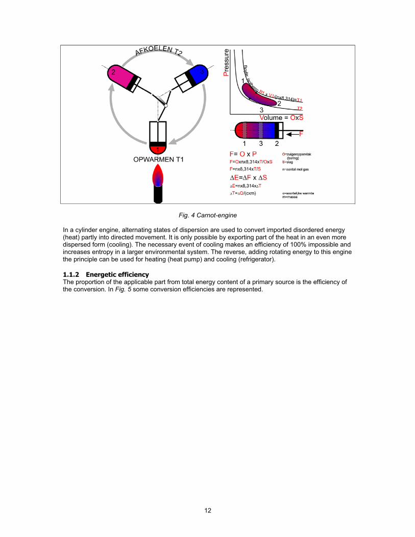
Fig. 4 Carnot-engine

In a cylinder engine, alternating states of dispersion are used to convert imported disordered energy (heat) partly into directed movement. It is only possible by exporting part of the heat in an even more dispersed form (cooling). The necessary event of cooling makes an efficiency of 100% impossible and increases entropy in a larger environmental system. The reverse, adding rotating energy to this engine the principle can be used for heating (heat pump) and cooling (refrigerator).

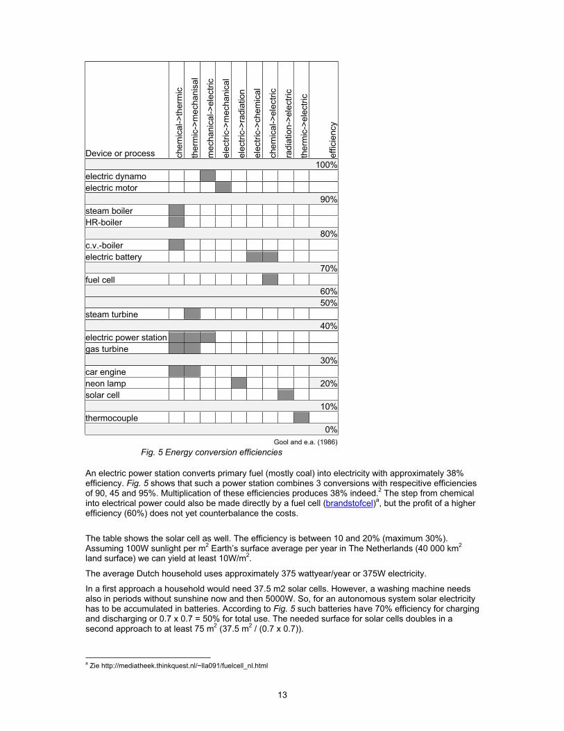
1.1.2 Energetic efficiency The proportion of the applicable part from total energy content of a primary source is the efficiency of the conversion. In Fig. 5 some conversion efficiencies are represented.

13

Device or process chem

ical->

therm

ic

therm

ic->

mecha

nis

al

mechanic

al->

ele

ctr

ic

ele

ctr

ic->

mecha

nic

al

ele

ctr

ic->

radia

tion

ele

ctr

ic->

chem

ical

chem

ical->

ele

ctr

ic

rad

iation

->ele

ctr

ic

the

rmic

->e

lectr

ic

eff

icie

ncy

100%

electric dynamo

electric motor

90%

steam boiler

HR-boiler

80%

c.v.-boiler

electric battery

70%

fuel cell

60%

50%

steam turbine

40%

electric power station

gas turbine

30%

car engine

neon lamp 20%

solar cell

10%

thermocouple

0%

Gool and e.a. (1986)

Fig. 5 Energy conversion efficiencies

An electric power station converts primary fuel (mostly coal) into electricity with approximately 38% efficiency. Fig. 5 shows that such a power station combines 3 conversions with respecitive efficiencies of 90, 45 and 95%. Multiplication of these efficiencies produces 38% indeed.

2 The step from chemical

into electrical power could also be made directly by a fuel cell (brandstofcel)a, but the profit of a higher

efficiency (60%) does not yet counterbalance the costs.

The table shows the solar cell as well. The efficiency is between 10 and 20% (maximum 30%). Assuming 100W sunlight per m

2 Earth’s surface average per year in The Netherlands (40 000 km

2

land surface) we can yield at least 10W/m2.

The average Dutch household uses approximately 375 wattyear/year or 375W electricity.

In a first approach a household would need 37.5 m2 solar cells. However, a washing machine needs also in periods without sunshine now and then 5000W. So, for an autonomous system solar electricity has to be accumulated in batteries. According to Fig. 5 such batteries have 70% efficiency for charging and discharging or 0.7 x 0.7 = 50% for total use. The needed surface for solar cells doubles in a second approach to at least 75 m

2 (37.5 m

2 / (0.7 x 0.7)).

a Zie http://mediatheek.thinkquest.nl/~lla091/fuelcell_nl.html

14

However, most domestic devices do not work on direct current (D.C.) from solar cells or batteries, but on alternating current (A.C.). The efficiency of conversion into alternating current may increase the needed surface of solar cells into 100 m

2 or 1000 W installed power. Supposed solar cells cost € 3,-

per installed W, the investment to harvest your own electricity will be € 3 000,-. In the tropics it will be approximately half.

Electricity from the grid amounts to € 0.70 per Wa. So, an average use of approximately 375 W electricity approximately amounts to € 250 per year. In this example the solar energy earn to repay time exclusive interest is already approximately 3000/250 per year = 12 year. Concerning peak loads it is better to cover only a part of the needed domestic electricity by solar energy and deliver back the rest to the electricity grid avoiding efficiency losses by charging and discharging batteries. It decreases the earn to repay time.

The costs of solar cells decreased since 1975 (€70 per installed watt) a factor of approximately 23 (€3). Their efficiency and the costs of fossile fuels will increase. To pass the economic efficiency of fossile fuels as well the price of solar cells has to come down relatively little (Fig. 6).

After Maycock cited by Brown, Kane et al. (1993)

Fig. 6 Decreasing costs of solar cells

The efficiency of solar cells is rather high compared with the performance of nature. Plants convert approximately 0.5 % of sunlight in temporary biomass (sometimes 2%, but overall 0.02%), from which ony a little part is converted for a longer time in fossile fuel. Biomass production on land delivers maximally 1 W/m

2 being an ecological disaster by necessary homogeneity. In a first approach a

human of 100 W would need minimally 100 m2 land surface to stay alive. However, by all efficiency

losses and more ecologically responsible farming one could better depart from 5000 m2 (half a

hectare).

1.1.3 Global energy There is more than 6 000 times as much solar power available as mankind and other organisms use. The Earth after all has a radius of 6Mm (6 378 km) and therefore a profile with approximately 128

Mm2 ( x 6 378 km x 6 378 km = 127 796 483 000 000 m

2) capturing sunlight. The solar constant

outside atmosphere measures 1 353 W/m2, on the Earth’s surface reduced to approximately 47% by

premature reflection (-30%) or conversion in heat by watercycle (-21%) or wind (-2%). The remainder (636 W x 127 796 483 000 000 m

2 of profile surface unequally distributed over the spherical surface)

is available for profitable retardation by life or man. However, 99.98% is directly converted into heat and radiated back to the universe as useless infrared light. Only a small part (-0.02%) is converted by other organisms in carbohydrates and since some billion years a very small part of that is stored more than a year as fossile fuel.

15

Earth The Netherlands

radius Mm 6

profile Mm2 128

spherical surface Mm2 509 0,10 0,02%

solar constant TW/Mm2 1353 832,99 61,57%

a

solar influx TW 172259 33,83 0,02%

from which available

sun 47% or 100W/m2 TW 80962 10,00b

0,01%

wind 2% TW 3445 0,68 0,02%

fotosynthesis 0,02% TW 34 0,01 0,02%

Fig. 7 Globally and nationally received solar power

The biological process of storage produced an atmosphere livable for much more organisms than the palaeozoic pioneers. Without life on earth the temperature would be 290

oC average instead of 13

oC.

Instead of nitrogen (78%) and oxigen (21%) there would be a warm blanket of 98% carbon dioxide (now within 100 years increasing from 0.03% into 0.04%). By fastly oxidating the stored carbon into atmospheric CO2 we bring the climate of Mars and heat death closer, unless increased growth of algas in the oceans keep up with us.

The actual energy use is negligible compared with the available solar energy (compare Fig. 7 and Fig. 8).


coal TW 3 0,02 0,45%

oil TW 4 0,03 0,77%

gas TW 2 0,05 2,14%

electricity TW 2 see fossile

traditional biomass TW 1

total TW 13 0,10 0,73%

Fig. 8 Gobal and national energy usec

Concerning Fig. 6, Fig. 7 and Fig. 8 making a plea for using wind or biomass is strange. Calculations of an ecological footprint based on surfaces of biomass necessary to cover our energy use have ecologically dangerous suppositions. Large surfaces of monocultures for energy supply like production forests (efficiency 1%) or special crops (efficiency 2%) are ecological disasters.

Without concerning further efficiency losses Dutch ecological footprint of 0.10 TW (Fig. 8) covered by biomass would amount 10 times the surface of The Netherlands yielding 0.01 TW (Fig. 7). However, covered by wind or solar energy it would amout 1/7 or 1/100. However, efficiency losses change these facors substantially (see 1.1.4).

To compare energy stocks of fossile fuels with powers (fluxes) expressed in terawatt in Fig. 7 and Fig. 8, Fig. 9 expresses them in power available when burned up in one year (a = annum).

a Cosine of latitude.

b Here 100W/m

2 is assumed.

c Dutch figures are more recent than global ones.

16


coal TWa 1137 0,65 0,06%

oil TWa 169 0,03 0,02%

gas TWa 133 1,60 1,20%

total TWa 1439 2,28 0,16%

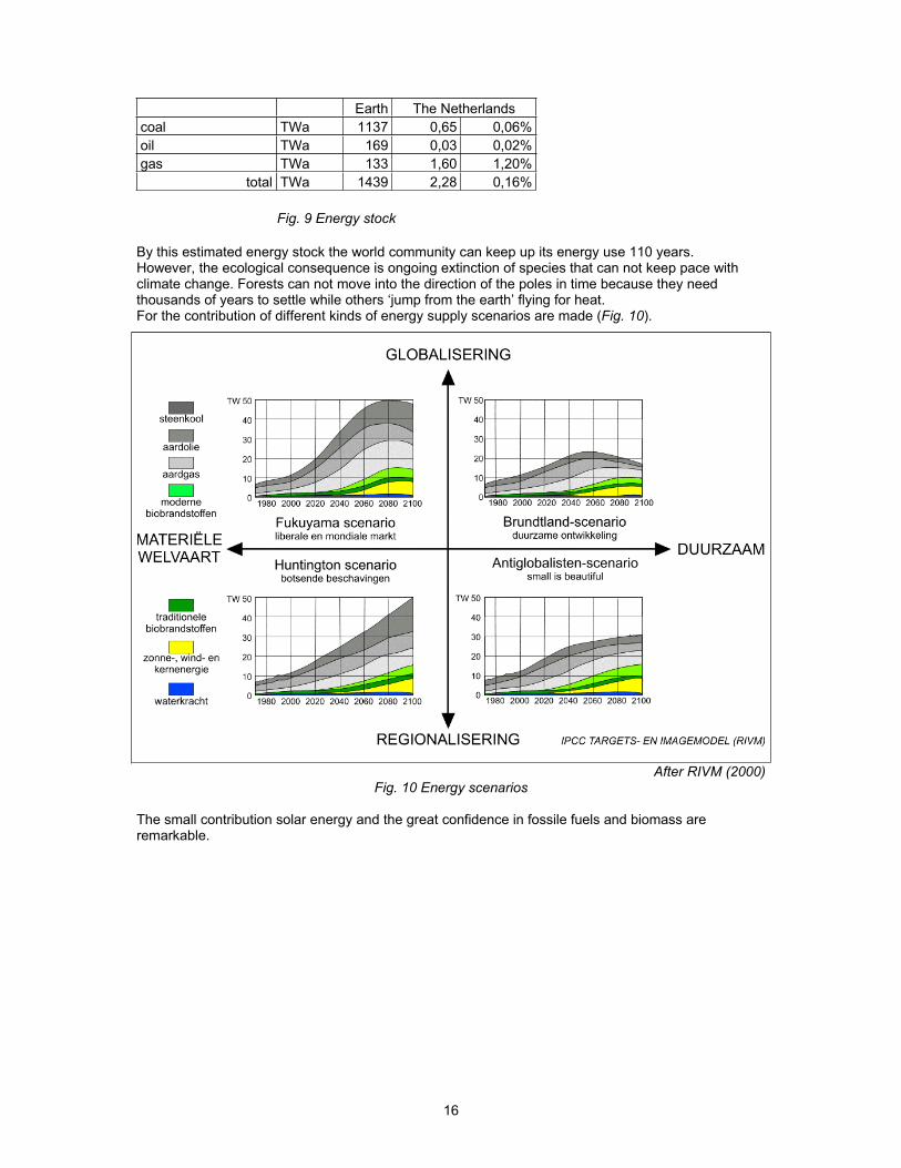
Fig. 9 Energy stock

By this estimated energy stock the world community can keep up its energy use 110 years. However, the ecological consequence is ongoing extinction of species that can not keep pace with climate change. Forests can not move into the direction of the poles in time because they need thousands of years to settle while others ‘jump from the earth’ flying for heat. For the contribution of different kinds of energy supply scenarios are made (Fig. 10).

After RIVM (2000) Fig. 10 Energy scenarios

The small contribution solar energy and the great confidence in fossile fuels and biomass are remarkable.

17

1.1.4 National energy According to CBS (2003) Dutch energy use (Fig. 11) approaches 0,1 TW (100 000 MW)

a from which

0.01TWeb.

Fig. 11 Development of Dutch energy use 1988-1998

An ecological footprint on the basis of nearly 7 times as much wind looks favourable, but how efficient wind can be harvested? How useful is the power of 680 000 MW (0,68 TW) blowing over The Netherlands? The technical efficiency of wind turbines is maximally 40%, practically 20%. The energy from wind principally can not be harvested fully because the wind then would stand still behind the turbine. At least 60% of the energy is necessary to remove the air behind the turbine fast enough. Technical efficiency alone (R1) increases the wind based footprint of 1/7 into more then ½. But there are other efficiencies (see Fig. 12) together reducing the available wind energy from 0,68 TW available into maximally 0.02 TW useful.

Putting the Dutch coast from Vlaanderen to Dollard full with a screen of turbines and behind it a second one and so on until Zuid Limburg, these screens could not be filled by more than 80% with circular rotors (R2). In the surface of the screen some space has to be left open between the rotors to avoid non productive turbulence of counteracting rotors (R3). In a landscape of increasing roughness by wind turbines the wind will choose a higher route. So, in proportion to the height the screens need some distance to eachother (R4). The higher the wind turbine, the higher the yield, but we will not harvest wind on heights where costs outrun profits too much (R5). Decreasing height could be compensated partly by increasing horizontal density (R6) though local objections difficult to be estimated here can force to decrease horizontal density (R7).

a http://www.cbs.nl/nl/cijfers/themapagina/energie/1-cijfers.htmb TWe is the electrical part. To convert 1 PJ/year (10

15 joule per year) as usual in CBS figures into MW (10

6 joule per second)

one should multiply by 31,7 (amongst others dividing by the number of seconds per year: 1015

/(106*365*24*60*60)).

18

R1 technical efficiency 0,20 R5 vertical limits 0,30

R2 filling reduction 0,80 R6 horizontal compensation 2,50

R3 side distance 0,25 R7 horizontal limits P.M.

R4 foreland distance 0,85 PRODUCT TOTAL 0,03

Fig. 12 Reductions on theoretical wind potential.

By these efficiency reductions the ecological footprint on basis of wind appears not to be 1/7, but at least 5. For an ecological footprint on the basis of solar energy there are only technical and horizontal limits. A comparable ecological footprint then is 1/10. In both cases efficiency losses should be added caused by storage, conversion and transport, but these are equal for both within an all-electric society.

The ecological footprint based on biomass depends on location bound soil characteristics and efficiency losses for instance by conversion into electricity. A total efficiency of 1% applied in the comparance of Fig. 13 is optimistic.

W/m2

rounded total Dutch energy use including 100000 MW 1,00

rounded Dutch electricity use 10000 MW 0,10

WIND

over The Nederlands blows at least 680000 MW 6,80

after reduction by 0.03 17340 MW 0,17

required surface 577%

SUN

The Nederlands receives 10000000 MW 100

after reduction by 0.1 1000000 MW 10


BIOMASS

The Nederlands receives 10000000 MW 100

after reduction by 0.01 100000 MW 1


Fig. 13 Comparing the yield of wind, sun and biomass

What are the costs? In Fig. 14 for wind, sun and biomass the required surface is represented only. The environmental costs are not yet stable. Environmental costs of new technologies are in the beginning always higher then later on. For coal, uranium and heavy hydrogen the environmental costs are calculated, the required surface is negligible (Jong, Moens et al. (1996)).

19

total per inh.

Actual Dutch energy use 95890 MW 5993 W

yielded by

solar cells 10 x 1000 km2 0,06 ha

wind 564 x 1000 km2 3,53 ha

biomass 96 x 1000 km2 0,60 ha

surface of The Nederlands inclusive Continental Plat 100 x 1000 km2 0,63 ha

Actual use electric 10432 MW 652 W

remaining heat 26080 MW 1630 W

yielded by

coal 20864 mln kg coal 1304 kg coal

waste 62592 mln kg CO2 3912 kg CO2

waste 835 mln kg SO2 52 kg SO2

waste 209 mln kg NOx 13 kg NOx

waste 1043 mln kg as 65 kg as

uranium 8346 kg uranium 0,001 kg uranium

waste 3452992 kg radio-active 0,216 kg radio-active

heavy hydrogen (fusion) 10432 kg h.hydrogen 0,001 kg h.hydrogen

waste 10432 kg helium 0,001 kg helium

Fig. 14 Environmental costs of energy use

The environmental costs of oil and gas are less than those of coal, but concerning CO2-production comparable: the total production is approximately 30kg per person per day! That makes clear we have to avoid the use of fossile fuels.

The contribution of non fossile fuels is increased substantially (Fig. 15), but it is not yet 1000 from the yearly used 100 000 MW. The growth of 0,5% into 0,8% is mainly due to the use of waste including biomass unused otherwise.

20

After CBS (2003)

Fig. 15 Contribution of sustainable energy sources 1990 en 1999

The growth of the contribution of wind, heat pumps and sun (Fig. 16) is impressive on itself, but not yet responsible for 0.1% of total energy use.

CBS (2003)

Fig. 16 Contribution of wind, sun and heat pumps between 1990 en 1999

Why develops solar energy so slowly while so much energy can be gained while solar cells are 23 times as cheap as 30 years ago? The fast decrease in price of Fig. 6 would be due to efficiency improvements in peripheral equipment. Just before passing the economic efficiency of fossile fuels

21

basic barriers loom up. Which basic barriers are that? The oil industry has collected patents and studies that question. Scenarios still depart from a small contribution of solar energy in 2030. The development of the steam engine lasted 40 years. Are the barriers larger? Any way, the consequences are larger than those of the industrial revolution. Many people will loose their jobs or investments, but use of energy, depletion of resources, mobility would no longer be environmental problems. Only basic ecological problems remain: from the 1.5 mln known species 100 000 are lost, 80% of the human population is not healthy.

1.1.5 Power supply Electric power stations in The Netherlands have a capacity of approximately 15 GWe (15 000 MWe),from which at average 10 GWe is used (the rest is necessary to receive peak loads). These plants produce in the same time approximately 15 GWth. From that heat only a small part is used. Electric power stations can not be switched off immediately. Temporary overproduction is sold cheaper at night or into foreign countries (for example to pump up water in storage reservoirs). Approximately 2% is generated by nuclear power, 1% sustainable, the rest by fossile fuels.

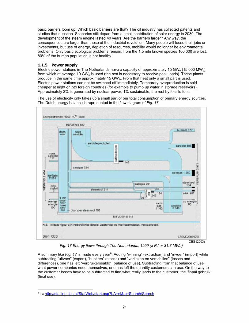
The use of electricity only takes up a small part of our total consumption of primary energy sources. The Dutch energy balance is represented in the flow diagram of Fig. 17.

CBS (2003)

Fig. 17 Energy flows through The Netherlands, 1999 (x PJ or 31.7 MWa)

A summary like Fig. 17 is made every yeara. Adding “winning” (extraction) and “invoer” (import) while

subtracting “uitvoer” (export), “bunkers” (stocks) and “verliezen en verschillen” (losses and differences), one has left “verbruikerssaldo” (balance of use). Subtracting from that balance of use what power companies need themselves, one has left the quantity customers can use. On the way to the customer losses have to be subtracted to find what really lands to the customer, the ‘finaal gebruik’ (final use).

a Zie http://statline.cbs.nl/StatWeb/start.asp?LA=nl&lp=Search/Search

22

Calculating back these figures per inhabitant, expressing them into the individual human power during a year (100 Wa), one gets a figure like the number of ‘energy slaves’ people have to their disposal. The balance of use comes down to 57 energy slaves per Dutch(wo)man. Power companies need 11 of them to produce the rest. So, 46 remain for final use. From these 46 energy slaves industry takes 19, transport 8 and 19 are needed for offices and dwellings. From these 19 natural gas delivers 13, oil 3 and electricity 3 as well.

In 1982 the average inhabitant had 11 energy slaves in his own home, 10 of them needed for heating. At that time there were 2.8 inhabitants per dwelling. So, at average approximately 3000 m3 natural gas per year was needed for heating a house.

1.1.6 Local energy storage Sustainable energy sources fluctuate per season or per 24 hour. That is why their supply does not stay in line with demand. Therefore, energy storage is of overriding importance for succes of these sources, but also for mobile applications like cars.

3

In Fig. 18 some kinds of storage are summed up with their use of space and efficiency. If you lift up 1000 kg water (1m

3) 1 meter against Earth’s gravity (9.81 m/sec

2), you need 1000 kgf or 9810 newton

during 1 m and 9810 newton*meter is 9810 joule or 0.0003109 watt during a year (Wa, see Fig. 1,page 9). Now you have got potential energy you can partly gain back as electricity any time you want by letting the water flow down via a water turbine and a dynamo. The efficiency is approximately 30%. So, you can gain back maximally some 0.000095 watt*year/m

3 electricity. If you have a basin of 1km

2

where you can change the waterlevel 1m you can deliver 95 Wea during a year, 190 We during half a

year or 34722 We (0.00003472 GWe) during a day. To deliver 1 GWe you need 1/ 0.00003472 km2 =

28800 km2 (see Fig. 18). That is nearly three-quarter of the Netherlands! A larger fall (of 10m for

example) improves both storage and efficiency of the turbine by increased speed of falling water.

Storage4 Efficiency Surface for 1 GWe during

gross (max.) net 24 hours half a year

Wa/m3 % Wa/m3 km2

km2

Potential energy

water (fall = 1 m) 0,0003 x30% =0,0001 28800 5259600

water (fall = 10 m) 0,003 x75% =0,002 1152 210384

water (100 m) 0,03 x90% =0,03 96 17532

50 atm. pressed air 1,3 x50% =0,6 4 789

Kinetic energy

fly weel 32 x85% =26,9 0,10 18,56

Chemical energy

natural gas 1 x80% =0,8 3,42 625,00

lead battery 8 x80% =6,3 0,43 78,89

hydrogen (liquid) 274 x40% =109,5 0,03 4,57

petrol 1109 x40% =443,6 0,01 1,13

Heat

water (70oC) 6 x40% =2,5 1,08 197,24

rock (500oC) 32 x40% =12,7 0,22 39,45

rock salts(850oC) 95 x40% =38,0 0,07 13,15

After Lysen (1980)and Hermans and Hoff (1982)

Fig. 18 Storage capacity (for conversion into electricity) from some systems

From the row ‘50 atm. pressed air’ on, the last column of Fig. 18 simply departs from a surface with a built height of 1m needed to deliver 1 GWe (1 000 MWe) during 24 hours or half a year continuously. By doubling the height of course you can halve the needed surface. Space for turbines and dynamos is not yet included. Fossile fuel like petrol still stores energy most efficiently.

a 1 GWe means "1 000 000 000 watt electric", the heat part is lost in efficiency reduction.

23

However, in normal storage circumstances this surface is estimated too large for two reasons. Firstly energy production by some differentiation of sources never falls out completely. So you can partly avoid storage. Secondly, the average time difference between production and consumption is smaller than half a year or 24 hours. So, you need a smaller capacity. However, you have to tune the capacity to peak loads and calculate a margin dependent on the risks of non-delivery you want to take. These impacts can be calculated as separate reductions of the required storage

The actual Dutch energy use amounts nearly 100 GW, partly converted into electricity. So, you do not need 100x the given surface per GW to cover this use from stock. After all, in the total figure losses of conversion from fuel into electricity are already calculated in, and these are calculated in Fig. 18 as well.

1.1.7 References to Energy Brown, L. R., H. Kane, et al. (1993) Vital Signs The trends that are shaping our future (London)

Earthscan Publications Ltd. CBS (2003) Homepage URL http://www.cbs.nl/. Gool, v. and e.a. (1986) Poly-energie zakboekje (Arnhem) Koninklijke PBNA. Hermans, L. J. F. and A. J. Hoff, Eds. (1982) Energie. Een blik op de toekomst. (Utrecht) Het

Spectrum. Jong, T. M. d., R. Moens, et al. (1996) Energie, water en mineralen Monografieen Milieuplanning SOM

25 (Delft) TUDelft Faculteit Bouwkunde: 128. Lysen, E. (1980) Eindeloze energie Alternatieven voor de samenleving (Utrecht) Het Spectrum B.V.

ISBN 90 274 5354 3. RIVM (2000) Insights for the third Global Environment Outlook from related global scenario anlayses

(Bilthoven).

1.2 Sun

1.2.1 Looking from the universe ( and latitude )The earth orbits around the sun in 366.25 days at a distance of 147 to 152 mln km. The radius of the earth is only maximally 6 378 km. So, the sunlight reaches any spot on earth by practically parallel rays. The surface covering that practically circular orbit is called the ecliptic surface. The polar axis of

the Earth has always an angle = 23,46o with any perpendicular on that ecliptic surface.

On December 22nd

(Fig. 19) the angle between polar axis and the line from Sun into Earth within the

ecliptic surface equals 90o+ . On March 21

st = 90

o, on June 21

st = 90

o- and on September 23

rd

again = 90o. Arrows a in Fig. 19 show the only latitudes where sunrays hit the Earth’s surface

perpendicular at December 22nd

and June 21st. So, the sunlight reaches the earth perpendicular only

between plus or minus 23,46o latitude from the equator (tropics). Anywhere else they hit the Earth’s

surface slanting. At December 22nd

the sunlight (sunray b in Fig. 19) does not even reach the north pole inside the arctic circle at 90

o – 23,46

o = 66, 54

o latitude (arctic night).

Fig. 19 The orbit of the earth around the sun

The sunlight reaching the earth’s atmosphere has a capacity of 1353 W/m2 (solar constant). Some 500

km atmosphere reduces it by approximately 50%. So, any m2 of sunrays reaching the surface of the

Earth distributes say 677 W over its slanting projection on the earth’s surface. In Fig. 20 (left) the solar capacity of 1m

2 (677W) is distributed that way over the larger surface SN. That 1 m

2 capacity divided

by hypotenuse surface SN equals cos( ). So, 1m2 Earth’s surface in P receives cos( ) x 677W.

Fig. 20 The received sunlight average per year at latitude ;daily fluctuations with the hour angle .

On March 21st or September 23

rd it happens 24 hours on the whole latitude circle because these

days polar axis is perpendicular to the sunrays. That circle with radius r of latitude (‘parallel’), seen

from the Sun is a straight line with 2r length. On both days the Sun continuously delivers cos( )*677W

25

on any m2 of that line. In 24 hours that capacity is distributed over a larger circular surface length 2 r

of the whole latitude circle. So, the 24 hour average is that capacity divided by . We do not yet have to calculate more cosinuses for every hour (Fig. 20 right) to conclude that 24 hour average. And March 21

st or September 23

rd offer useful averages for the whole year as well.

1.2.2 Looking from the Sun (culmination and declination )The University of Technology in Delft is positioned around 52

o latitude, a global parallel crossing the

building for Electrotechnical and Civil Engineering on its campus. The cosine of 52o is 0.616. So, there

the year average solar capacity at noon is 417 W per square meter earth surface. Averaged again per

24 hours it is 417/ = 133 W (not concerning Dutch weather conditions). This value is reached only as daily average on March 21

st or September 23

rd. At other dates it varies symmetrically around that

average. The day period between sunrise and sunset varies and throughout the year the sunlight

reaches the earth’s surface at noon by a varying maximum angle (‘culmination’ related to the Earth’

surface, not to be confused by declination related to its polar axis, see Fig. 22). After all, seen from the sun the earth nods ‘yes’ (Fig. 21). Bending to left and right does not matter for locally received sunrays.

Fig. 21 The yearly nodding earth with a parallel =52o seen from the sun.

December 22nd

the earth is maximally canted = 23.46o backwards related to the sunrays. At noon

we receive: 677 * cos(52o

+ ) = 170 W/m2. Canting forward on June 21

st we have to subtract :

677 * cos(52o

– ) = 595 W/m2. Inbetween we need a variable ‘declination’ { | +23.46

o–23.46

o}

instead of . In Fig. 22 declination is positive in June, so now we can write 677 * cos( – ) W/m2 for

any day at noon at any latitude. From Fig. 22 we can derive visually: + - = 90o or - = 90

o - .

Fig. 22 Declination

Declination could be read from Fig. 22 or calculated according to Voorden (1979) by = 23.44 sin(360

o x (284 + Day) / 365). As ‘Day’ we fill in for instance:

26

Mar21 = 31 + 28.25 + 21 = 80.25 Jun21 = 31 + 28.25 + 31 + 30 + 31 + 21 = 172.25 Sep21 = 31 + 28.25 + 31 + 30 + 31 + 30 + 31 + 31 + 21 = 264.25 Dec22 = 31 + 28.25 + 31 + 30 + 31 + 30 + 31 + 31 + 21 + 31 + 30 + 22 = 356.25

1.2.3 Looking back from Earth (azimuth and sunheight) But how is that capacity distributed per hour? The earth turns 360

o in 24 hours ousting the Old World

by the New Word all the time. That is 15o per hour, drawn in Fig. 21 (left) by 12 visible meridians of

15o.

The distribution on a constant latitude is not only affected by a declination varying day by day but

also by the hour angle visibly varying every minute. From Fig. 23 we derive the hour angle of sunset

and sunrise: cos( sunset)= h x cot( )/r x cos( ), while h = r*sin( ).

Fig. 23 Sunset and sunheight at noon varying with

and hour angle on one parallel circle.

Fig. 24 Looking back to the universe in the Autumn.

Within that formula, r plays no rôle and cot( ) = tan (90o – ) = tan( ), see Fig. 22. So, we can write:

sunrise = acos(sin( ) x tan( ) / cos ( )) / 15o and sunset = 24 hour - sunrise.

Now we can move our field of vision down to earth looking back to the universe as Copernicus saw it, reconstructing the preceding model from what he saw. Then we see any star moving daily in perfect circles around, the Pole Star (Polaris) standing still. So, we see the Great Bear and some ‘circumpolar’ constellations througout the year turning around Polaris (Fig. 24). Other constellations disappear daily behind the horizon, be it seasonly at an other moment of the day and therefore in some seasons by day not visible behind the brightness of the Sun. Polaris is a star 1600 times more powerful than the Sun, but on a distance of 300 light years. Occasionally it stands in our polar axis apparently standing still that way, moving too little (1 degree) to take into account.

The Sun makes its daily circles shifting approximately 1 degree per day (the year circle of 360o is

called eclipse) against a more stable remote background of 12 constellations (the Zodiac), according to its yearly wave seen by a nodding Earth. Turning ourselves 360

o we see a lamp on our desk describing a circle around us as well. Bowing our

head backward 23.46o while turning around we see the lamp low in our field of vision. When we stay

turning around and in the same time walk around the lamp keeping our head in the same polar direction (slowly nodding forward until we are half way and than again backward) we experience how we see the sun during the year starting from December 22

st. When we had a third eye in our mouth we

would have a complementary view from the southern hemisphere as well.

27

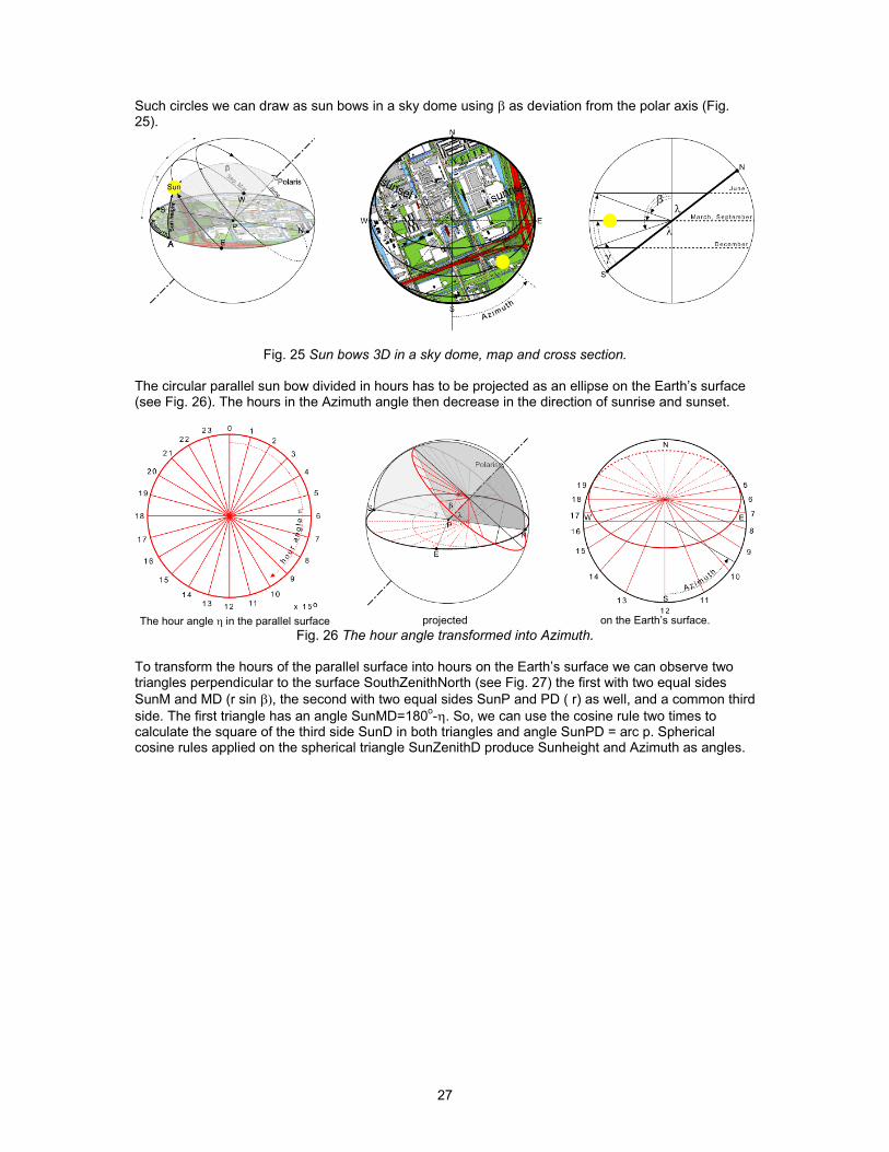
Such circles we can draw as sun bows in a sky dome using as deviation from the polar axis (Fig. 25).

Fig. 25 Sun bows 3D in a sky dome, map and cross section.

The circular parallel sun bow divided in hours has to be projected as an ellipse on the Earth’s surface (see Fig. 26). The hours in the Azimuth angle then decrease in the direction of sunrise and sunset.

The hour angle in the parallel surface projected on the Earth’s surface.

Fig. 26 The hour angle transformed into Azimuth.

To transform the hours of the parallel surface into hours on the Earth’s surface we can observe two triangles perpendicular to the surface SouthZenithNorth (see Fig. 27) the first with two equal sides

SunM and MD (r sin , the second with two equal sides SunP and PD ( r) as well, and a common third

side. The first triangle has an angle SunMD=180o- . So, we can use the cosine rule two times to

calculate the square of the third side SunD in both triangles and angle SunPD = arc p. Spherical cosine rules applied on the spherical triangle SunZenithD produce Sunheight and Azimuth as angles.

28

Cosine rule: a

2 = b

2 + c

2 - 2bc cos A

Spherical cosine rule: cos a = cos b cos c+ sin b sin c cos A

Fig. 27 Two isosceles triangles and a spherical one

However, Voorden (1979) in his Appendix A and C (see Enclosure 2) derives by more difficult transformation rules the usual and easier formulas:

Declination = 23.44o x sin(360

o x (284+Day)/365))

Sunheight= asin(sin(Latitude) sin(Declination(Day)) – cos(Latitude) cos(Declination(Day) cos(Hour x 15

o)

Azimuth= asin(cos(Declination(Day) sin(Hour x 15o))/cos(Sunheight(Latitude, Day, Hour))

1.2.4 Time on Earth On a meridian 1

o East of us (68 km on our latitude) local solar time is already 4 minutes later. If we

used the solar time of our own location we could only make appointments with persons living on the same meridian. So, we agreed to make zones East from Greenwich of ± 7.5

o around multiples of 15

o

(1026 km on our latitude), using the solar time of that meridian. However, between the weekends closest to April 1

st an November 1

st we save daylight in the evening by using summertime. By adding

an hour around April 1st in the summer, 21.00h seems 22.00h on our watch and it is unexpectedly light

in the evening. So, to find the solar time from our watch we have to subtract one hour in the summer and the number of degrees of longitude x 4 minutes West of the agreed meridian. In the Netherlands we use the solar time of 15

o East of Greenwich (time zone 1), but live between 3

o and 8

o.

29

http://www.squ1.com/index.php?http://www.squ1.com/solar/solar-position.htmlFig. 28 Time zones

So, on the Faculty of Architecture in Delft (4o 22.5’ easter longitude = 4.38

o) in winter we have to

subtract 15 x 4 minutes from our watch time and add 4.38 x 4 minutes (-10.62o x 4 minutes = -48.48

minutes) to find an approximate solar time. In summertime we have to subtract an extra hour.

In addition to these corrections we have to add or subtract some minutes (time equalization E) amongst others due to differences in travel speed (29.3 km/s in summer, 30.3 km/s in winter) around the Sun according to Fig. 29.

Day ..0 365

0 30 60 90 120 150 180 210 240 270 300 330 360 390

20

18

16

14

12

10

8

6

4

2

0

2

4

6

8

10

12

14

16

18

20

E( )Day

Day

E( )Day .9.87 sin ..4

364( )Day 81 .7.53 cos .

.2

364( )Day 81 .1.5 sin .

.2

364( )Day 81

Fig. 29 Time equalization per day of the year

So, instead of the Hour we read on our watch (WHour with minutes decimally added) in the formulas for Sunheight and Azimuth we should fill in Sun Hour (SHour) from:

SHour(WHour,Timezone,Longitude,Summertime,Day) = WHour - Timezone + Longitude/15o – Summertime + E(Day)/60

As Timezone we fill in 1, 2, 3 and so on with a maximum of 23. As Summertime we fill in daylight saving yes=1, no=0 and E(Day) we read or calculate from Fig. 29.

30

Finally, atmospheric refraction of 34’ and sun radius of 16’ (together nearly 1o) shows us sunrise

nearly 4 minutes earlier and sunset 4 minutes later, but by day this effect approaches to zero at noon.

1.2.5 Calculating sunlight periods Putting the formulas we found in an Excel Sheet (download http://www.bk.tudelft.nl/urbanism/team,publications 2003 Sunsheet), we can check them by observing shadows.

Input

Date Time Latitude Longitude

Date Days Hour Minute Degrees Minute Degrees Minute Timezone Summertime

18-apr-03 108,25 11 45 52 0 4 30 1 yes

Fig. 30 Data needed for solar calcuations

We need date, time, geographical coordinates, the time zone and wether or not we have to take summer time into account. The Sheet brings them into a decimal form and adds a time correction to calculate the hour angle in radians. Excel needs radians to calculate sine, cosine and tangent.

Calculated hour h m deg rad

Watch time 11,75 11 45

TimeCorrection -1,69 -2,00 19

Sunhour 10,06 10 4

Hour angle 151 2,63

Timezone 1

Summertime 1

Latitude 52,00 0,91

Longitude 4,50 0,08

Fig. 31 Restating data in dimensions needed

The sheet then calculates the declination of the day and at what time on our watch we can expect sunrise, culmination and sunset neglecting atmospheric influence from –4 to + 4 minutes. Finally the sheet calculates Azimuth and Sunheight. Azimuth is calculated from South, but a compass gives the number of degrees from North (180 – Azimuth).

31

Calculated hour h m deg rad

Declination 10,6 0,18

Watch Sunrise 6,77 6 46

Watch Culmination 13,69 13 41

Watch Sunset 20,61 20 37

Azimuth 40 0,70

On Compass (180 - Azimuth) 140

Sunheight 42 0,74

Prediction

Height 10,00

Shadow 10,97

Fig. 32 Solar calculations

The height of an object on the Earth’s surface given, the sheet calculates the length of its shadow. Now we can check these results by putting a pencil in the sun. Measure its height, the length of its shadow and Azimuth as the angle of its shadow with a North-South line (using a map or reliable compass, not disrupted by iron in the neighbourhood!) (Fig. 33).

Fig. 33 Fast indoor check of shadow.

Outdoors you can measure angles copying, folding and cutting the paper instrument of Fig. 34 to get the sunheight and the height of buildings. To measure height of buildings you need a mirror or mirroring piece of glass. Measuring Azimuth you need a compass or map as well.

32

Fig. 34 Measuring Azimuth, sunheight and building height outdoors

Fig. 34 shows a compass directed to the sun by adjustment to the shadow line of a vertical object. It indicates 106

o from North, which is 74

o from South (Azimuth). Sunheight appears to be 39

o on the

paper instrument. Turning the instrument 180o partly covered by a piece of glass we read an angle of

40o (tangent 0.84) to the upper edge of the mirrored building. According to our distance meter that

building is at 8.37m distance. However, when we measure it by tape measure it appears to be 10.30m, occasionally just like the shadow . So, we do not trust the electronic divice. It apparently has measured the tree closer by. The height of the building must be 10.30 x 0.84 = 8.65m above the table surface from which we took the measurement (35cm above ground level). So, the building should be 9m high. That could be right, because the building has 2 storeys (3 layers). Now we can fill in the measurements in http://www.bk.tudelft.nl/urbanism/team, publications 2003 Sunsheet.xls (Fig. 35) and check its prediction.

33

date 09-06-03 dd-mm-yy

Watch time 10.15 hour.minute

Building height 9 metres

Shadow 10.30 metres

Azimuth 74 degrees

Sun height 39 degrees

Building height and Shadow would indicate (calculated):

Azimuth 74 1.29

degrees radians

Sunheight 41 0.79

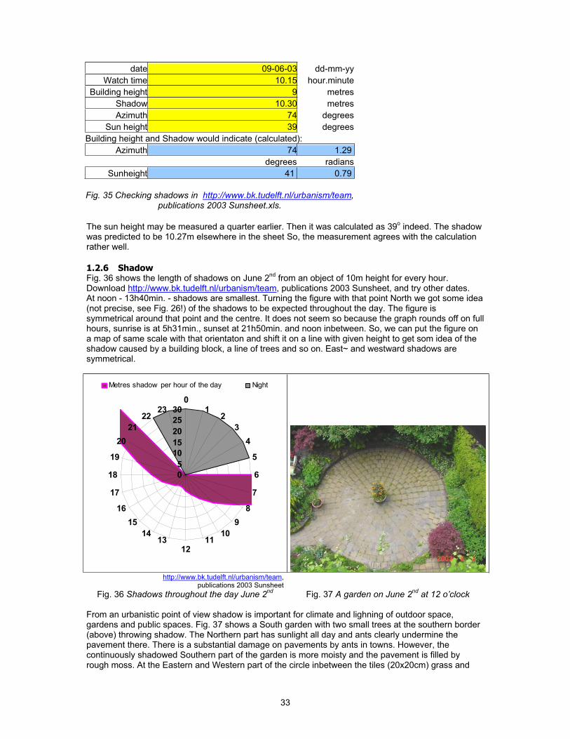
Fig. 35 Checking shadows in http://www.bk.tudelft.nl/urbanism/team,publications 2003 Sunsheet.xls.

The sun height may be measured a quarter earlier. Then it was calculated as 39o indeed. The shadow

was predicted to be 10.27m elsewhere in the sheet So, the measurement agrees with the calculation rather well.

1.2.6 Shadow Fig. 36 shows the length of shadows on June 2

nd from an object of 10m height for every hour.

Download http://www.bk.tudelft.nl/urbanism/team, publications 2003 Sunsheet, and try other dates. At noon - 13h40min. - shadows are smallest. Turning the figure with that point North we got some idea (not precise, see Fig. 26!) of the shadows to be expected throughout the day. The figure is symmetrical around that point and the centre. It does not seem so because the graph rounds off on full hours, sunrise is at 5h31min., sunset at 21h50min. and noon inbetween. So, we can put the figure on a map of same scale with that orientaton and shift it on a line with given height to get som idea of the shadow caused by a building block, a line of trees and so on. East~ and westward shadows are symmetrical.

0

5

10

15

20

25

300

12

3

4

5

6

7

8

9

1011

1213

14

15

16

17

18

19

20

21

2223

Metres shadow per hour of the day Night

http://www.bk.tudelft.nl/urbanism/team,publications 2003 Sunsheet

Fig. 36 Shadows throughout the day June 2nd

Fig. 37 A garden on June 2nd

at 12 o’clock

From an urbanistic point of view shadow is important for climate and lighning of outdoor space, gardens and public spaces. Fig. 37 shows a South garden with two small trees at the southern border (above) throwing shadow. The Northern part has sunlight all day and ants clearly undermine the pavement there. There is a substantial damage on pavements by ants in towns. However, the continuously shadowed Southern part of the garden is more moisty and the pavement is filled by rough moss. At the Eastern and Western part of the circle inbetween the tiles (20x20cm) grass and

34

flatter kinds of moss find their optimum. In the sunny Northern side sun loving plants like grape (Fig. 38 left) find their optimum, in the Southern shadowed borders you find shadow loving plants like ferns (Fig. 38 middle).

Fig. 38 Full sun, filtered shadow and full shadow On the other side of the building (Fig. 38 right) there is full shadow all day with high trees catching light in their crowns only and slow growing compact shrubby vegetation in a little front garden. Such fully shadowed spaces are suitable for parking lots. “Keep pavements in the shadow” may be a sound rule.

Trees filter sunlight by small openings projecting images of the sun on the ground as Minnaert noted in the first article of his marvellous book in three volumes on physics of the open air. You can see it best when an eclipse of the sun is projected thousendfold on the ground (Fig. 39). Most solar images are connected to vague spots and sometimes the openings in the foliage are too large to get clear images. Leaves of a tree are composed differently into a so called leaf mozaic (Fig. 40).

Fig. 39 Eclipse of the sun August 11th 1999 Fig. 40 Leaf mozaic

That roof of public space is worth more attention. People love the clairobscur of filtered light with local possibilities of choice for full sun and full shadow meeting their moods. It challenges their eyes more then one of the extremes continuously. Urban designers should be aware of the importance of light and its diversity in cities. None of them ever makes a shadow plan, though any painter knows that shadow makes the picture. The same goes for artificial city light in the evening and at night. Dry engineers calculate the minimum required amount of light for safety to disperse streetlamps as equally (economically) as possible over public space.

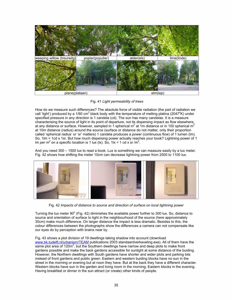
Nature’s diversity is primarily based on competition for light. Some plants grow as high as possible to outrun neighbours. Others are satisfied by less light growing slower, using more years to reproduce. By very closed foliage some trees do not leave any light to plants on the ground like spruces and beeches. They are the trees of dark forests. Trees of light forests are not stingy with light for plants growing below, like birches. They need helpers there to get the right minerals from soil. So, trees are different in light permeability (Fig. 41).

35

weeping willow (treurwilg) poplar(populier) alder(els) lime(linde)

plane(plataan) elm(iep)

Fig. 41 Light permeability of trees

How do we measure such differences? The absolute force of visible radiation (the part of radiation we call ‘light’) produced by a 1/60 cm

2 black body with the temperature of melting platina (2047

oK) under

specified pressure in any direction is 1 candela (cd). The sun has many candelas. It is a measure characterising the source of light in its point of departure, not its dispersing impact as flow elsewhere, at any distance or surface. However, sampled in 1 spherical m

2 at 1m distance or in 100 spherical m

2

at 10m distance (radius) around the source (surface or distance do not matter, only their proportion called ‘spherical radius’ or ‘sr’ matters) 1 candela produces a power (continuous flow) of 1 lumen (lm). So, 1lm = 1cd x 1sr. But how much dispersing power actually reaches your book? Lightning power of 1 lm per m

2on a specific location is 1 lux (lx). So, 1lx = 1 cd x sr /m

2.

And you need 300 – 1500 lux to read a book. Lux is something we can measure easily by a lux meter. Fig. 42 shows how shifting the meter 10cm can decrease lightning power from 2500 to 1100 lux.

Fig. 42 Impacts of distance to source and direction of surface on local lightning power

Turning the lux meter 90

o (Fig. 42) diminishes the available power further to 300 lux. So, distance to

source and orientation of surface to light in the neighbourhood of the source (here approximately 30cm) make much difference. On larger distance the impact is less dramatic. Besides to this, the colour differences between the photographs show the differences a camera can not compensate like our eyes do by perception with brains near by.

Fig. 43 shows a plot division of 19 dwellings taking shadow into account (download www.bk.tudelft.nl/urbanism/TEAM publications 2003 standaardverkaveling.exe). All of them have the same plot area of 120m

2, but the Southern dwellings have narrow and deep plots to make front

gardens possible and make the back gardens accessible for sunlight at some distance of the buiding. However, the Northern dwellings with South gardens have shorter and wider plots and parking lots instead of front gardens and public green. Eastern and western buiding blocks have no sun in the street in the morning or evening but at noon they have. But at the back they have a different character. Western blocks have sun in the garden and living room in the morning, Eastern blocks in the evening. Having breakfast or dinner in the sun attract (or create) other kinds of people.

36

Jong (2001) Hotzan (1994)Fig. 43 Plot division taking shadow into

account Fig. 44 Avoiding shadow by neigbours according to

German regulations

The value of dwellings can decrease when neigbours are not limited in building on their plots by regulation removing sun from other gardens. So, many urban plans regulate building on private plots.

1.2.7 References Sun Hotzan, J. (1994) DTV-Atlas Stadt. Von den ersten Gründungen bis zur modernen Stadtplanung

(München) Deutscher Taschenbuch Verlag GmbH&Co. ISBN 3-423-03231-6. Jong, T. M. d. (2001) Standaardverkaveling 11.exe. Voorden, M. v. d. (1979) Bezonning. Stedebouwfysica gc 49 (Delft) Technische Hogeschool Delft,

afdeling der Civiele Techniek: 70.

37

1.3 Temperature

1.3.1 Long term variation The power of the sun fluctuated in periods of 100 000 years or less, causing ice ages and great differences in wind, water, earth and life stored and named in layers of soil (Fig. 45).

Sticht.Wetensch.Atlas_v.Nederland (1985)page 13

Fig. 45 Temperature fluctuations in The Netherlands in the past 3 million years

These impacts are readable from the topographic history of The Netherlands (Fig. 46).

38

-200000 -150000 -75000 -40000 -10000

-5500 -4100 -3000 -2100 -1000

-200 600 1000 vloed 1000 eb 1100

1300 1550 1675 1800 1850

1930 1960 1989 Universiteit van Utrecht 1987 commisioned by Nederland Nu Als Ontwerp

Fig. 46 De topographic history of The Netherlands

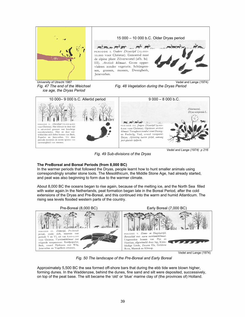
The Dryas and Alleröd Periods (from 10,000 years BC) In the famous Lascaux caves, people have made images of mammoths and long haired rhinos. These animals became extinct during the last Ice Age. In Scandinavian countries this period is known as Weichsel and in the Alpine countries as Würm. A tundra plant ‘dryas octopetala’ grew in our part of Europe at that time and gave its name to the last cold period of the Weichsel.

39

15 000 – 10 000 b.C. Older Dryas period

University of Utrecht 1987 Vedel and Lange (1974)

Fig. 47 The end of the Weichsel ice age, the Dryas Period

Fig. 48 Vegetation during the Dryas Period

10 000– 9 000 b.C. Alleröd period 9 000 – 8 000 b.C.

Vedel and Lange (1974) p 216

Fig. 49 Sub-divisions of the Dryas

The PreBoreal and Boreal Periods (from 8,000 BC)In the warmer periods that followed the Dryas, people learnt how to hunt smaller animals using correspondingly smaller stone tools. The Mesolithicum, the Middle Stone Age, had already started, and peat was also beginning to form due to the warmer climate.

About 8,000 BC the oceans began to rise again, because of the melting ice, and the North Sea filled with water again.In the Netherlands, peat formation began late in the Boreal Period, after the cold extensions of the Dryas and Pre-Boreal, and this continued into the warm and humid Atlanticum. The rising sea levels flooded western parts of the country.

Pre-Boreal (8,000 BC) Early Boreal (7,000 BC)

Vedel and Lange (1974)

Fig. 50 The landscape of the Pre-Boreal and Early Boreal

Approximately 5,500 BC the sea formed off-shore bars that during the ebb tide were blown higher, forming dunes. In the Waddenzee, behind the dunes, fine sand and silt were deposited, successively, on top of the peat base. The silt became the ‘old’ or ‘blue’ marine clay of (the provinces of) Holland.

40

University of Utrecht(1987) Vedel and Lange (1974)

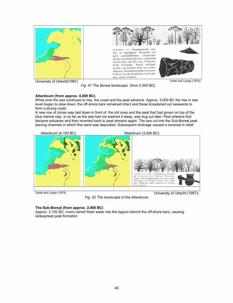
Fig. 51 The Boreal landscape. (from 5,500 BC)

Atlanticum (from approx. 4,000 BC)While ever the sea continues to rise, the coast and the peat advance. Approx. 3,000 BC the rise in sea level began to slow down; the off-shore bars remained intact and these broadened out seawards to form a strong coast. A new row of dunes was laid down in front of the old ones and the peat that had grown on top of the blue marine clay, in so far as the sea had not washed it away, was dug out later. Peat streams first became estuaries and then reverted back to peat streams again. The sea cut into the Sub-Boreal peat leaving channels in which fine sand was deposited. Subsequent drainage caused a reversal in relief.

Atlanticum (4,100 BC). Atlanticum (3,000 BC)

Vedel and Lange (1974) University of Utrecht (1987)tFig. 52 The landscape of the Atlanticum.

The Sub-Boreal (from approx. 2,000 BC)Approx. 2,100 BC, rivers carred fresh water into the lagoon behind the off-shore bars, causing widespread peat formation

41

University of Utrecht (1987) and Vedel and Lange (1974)

Fig. 53 The sub-Boreal landscape.

Late Boreal and Sub-Atlanticum, from 1000 BC.Approx. 1,000 BC: The stagnation of water from streams also causes hoogveen (i.e. peat formations above the water table) to develop on the lower parts of sandy ground (e.g., the Peel and Drente).Approx. 200 BC: peat erosion also occurs along the shores of the Almere lake (Zuiderzee area), thereby extending the lake.

Late Sub-Boreal, 1000 BC Sub-Atlanticum, 200 BC

Vedel and Lange (1974) University of Utrecht (1987)Fig. 54 The Sub-Boreal landscape and subatlanticum

The Roman period and early Middle Ages, from 100 BC.Approx. 100 BC: The sea attacked again and large areas of the laagveen (i.e. peat formations below the water table) were washed away: this continued for centuries. Bloemers, Kooijmans et al. (1981) and Klok and Brenders (1981) describe Roman relics from this period in The Netherlands like Corbulogracht (Fig. 56).Approx. 600 AD: The sea first broke through in the North to create the Waddenzee and the Zuiderzee.

42

University of Utrecht Bloemers, Kooijmans et al. (1981) page 99

Fig. 55 The landscape of the Early Middle Ages, 600 AD.

Fig. 56 Roman sites

1.3.2 Seasonal variation Latitudinal differences account for the largest global variations (from approx. -40°C to 30°C) in average monthly temperatures (Fig. 57 and Fig. 58).

Wolters-Noordhof (2001) page 180

Fig. 57 Global winter temperatures Fig. 58 Global summer temperatures

Latitudinal differences account for most of the average monthly temperature variations in Europe, but these are moderated by the sea from approx. -15°C to 25°C (Fig. 59 and Fig. 60).

43


Fig. 59 Winter temperatures in Europe Fig. 60 Summer temperatures in Europe

Latitudinal differences account for most of the average monthly temperature variation in the Netherlands, but they are moderated by the sea, especially in winter, from approx. 3°C to 17°C (Fig.61 and Fig. 62).


Fig. 61 Winter temperatures in the Netherlands Fig. 62 Summer temperatures in the Netherlands

In the Netherlands, on 3rd March 1976, the differences in local temperatures, within metres of each other, ranged from -2°C to 62°C (Fig.34). The air temperature at a height of 1 metre (Fig. 63) was 11.8°C.

44

Barkman and Stoutjesdijk (1987) citing Stoutjesdijk (1977)Fig. 63 Surface temperatures along a line perpendicular to edge of a forest

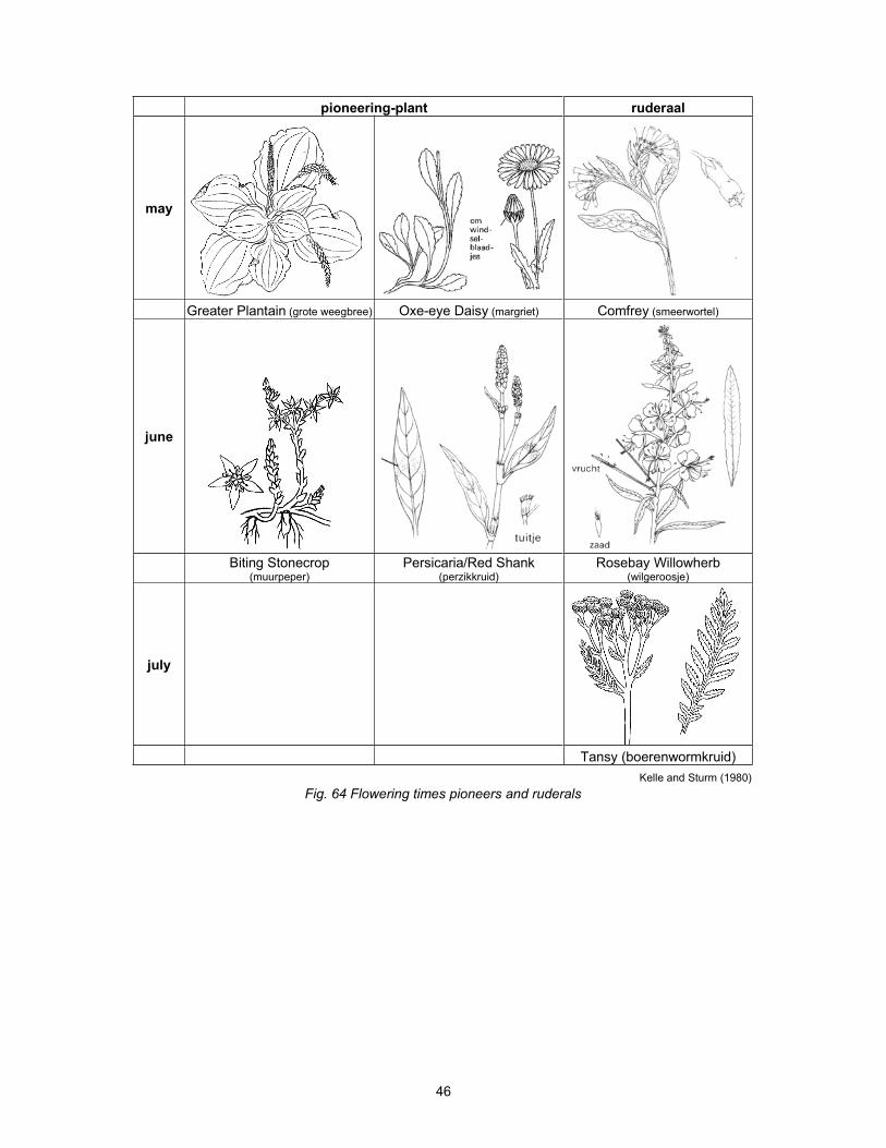
There are few pioneering plants that begin to flower in July, and, likewise, there are few plants growing on rough ground that flower before March; few trees flower after May and few shoreline and water plants before this month. In the table below, a number of plants are mentioned in the month in which they can first be encountered in the Netherlands.

45

pioneering-plant ruderaal

jan

Chickweed (vogelmuur) Groundsel (klein kruiskruid)

feb

Common Whitlowgrass (vroegeling) Coltsfoot (klein hoefblad)

march

Shepherd’s-purse (herdertasje) Purple Dead-nettle (paarse

dovenetel) Giant Butterbur (groot hoefblad)

april

Dandelion (paardebloem) Rape (koolzaad) Cow Parsley (fluitekruid)

46

pioneering-plant ruderaal

may

Greater Plantain (grote weegbree) Oxe-eye Daisy (margriet) Comfrey (smeerwortel)

june

Biting Stonecrop(muurpeper)

Persicaria/Red Shank(perzikkruid)

Rosebay Willowherb(wilgeroosje)

july

Tansy (boerenwormkruid)

Kelle and Sturm (1980)

Fig. 64 Flowering times pioneers and ruderals

47

grass land wood/forest

jan

Daisy (madeliefje) Hazel (hazelaar) Snow Drop (sneeuwklokje)

feb

Lesser Celandine (speenkruid) Alder (zwarte els) Cornelian Cherry (gele kornoelje)

march

Ground Ivy (hondsdraf) Silver Birch (ruwe berk) Wood Anenome (bosanemoon)

april

Lady’s Smock/ Cuckooflower(pinksterbloem) Poplar (populier) Broom (brem)

48

grass land wood/forest

may

Meadow Buttercup(scherpe boterbloem) Common Oak (zomereik) Herb-Robert (robertskruid)

june

Tormentil (tormentil) Wild Honeysuckle(wilde kamperfoelie)

july

Water Mint (watermunt) Hop (hop)


Fig. 65 Flowering times on grass land and in forest

49

wetand water

may

Yellow Iris/Yellow Flag(gele lis)

Yellow Water-lily(gele plomp)

june

Bulrush (lisdodde) Arrowhead (pijlkruid)

july

Common Reed (riet) Spiked Water-milfoil

(aarvederkruid)


Fig. 66 Flowering periods wetland and water

The plants listed above occur so widely that it is well worth while getting to know them. If one comes across pioneer vegetation in a certain season, then one can assume that the ground has been recently disturbed. If one comes across plants that grow on rough ground, then one can assume that the soil was disturbed one or more years previously. If one encounters woodland vegetation, then the soil has remained undisturbed for a longer time. Grassland plants indicate frequent mowing, however, from the nature of grassland vegetation and on the basis of the above table, one should be cautious about drawing conclusions regarding the mowing period.

5

50

Londo (1987) page 103

Fig. 67 The effect of mowing on various species. (Londo 1987: 103)

For more than 10 years already there has been a mowing policy in Zoetermeer that is directed towards ensuring that the food content of roadside vegetation is drastically reduced by regularly removing biomass:

Vos (1990)

Fig. 68 Mowing management in Zoetermeer

Over a period of 10 years, impoverishing the soil does not appear to lead to a large increase in the number of species growing there. Obviously, more time is needed for this to happen.

51

1.3.3 Daily variation Plants receiving shadow throughout the day in the growing seasons grow larger and narrower then the same species receiving more sunlight. They look for light rising as high they can. Plants are long term indicators of local climate (sun, wind, water, soil) while occasional measurements give a random indication of moments.

Vogel, Günter et al. (1970) page 198, 199

Fig. 69 The influence of variations in light

1.3.4 References Temperature Barkman, J. J. and P. Stoutjesdijk (1987) Microklimaat, vegetatie en fauna (Wageningen) Pudoc

Wageningen ISBN 90-220-0917-3. Bloemers, J. H. F., L. P. Kooijmans, et al. (1981) Verleden land (Amsterdam) Meulenhoff Informatief

ISBN 90-290-9992-5. Kelle, A. and H. Sturm (1980) Prisma Plantengids (Utrecht/Antwerpen) Uitgeverij Het Spectrum. Klok, R. H. J. and F. Brenders (1981) Reisboek voor Romeins Nederland en België

(Haarlem/Antwerpen) Fibula-Van Dishoeck/Standaarduitgeverij ISBN 90-228-3614-2. Londo, G. (1987) Natuurtuinen en -parken (Zutphen) B.V. W.J. Thieme & Cie ISBN 90-03-95000-8. Sticht.Wetensch.Atlas_v.Nederland (1985) Atlas van Nederland. Deel 13. Geologie (Den Haag) SDU

ISBN 90-12-05013-8. Vedel, H. and J. Lange (1974) Bomen en struiken in bos en veld (Baarn / Antwerpen) Moussault's

Uitgeverij Standaard Uitgeverij. Vogel, Günter, et al. (1970) Sesam atlas bij de biologie (Baarn) Bosch en Keuning ISBN

90.246.6909.x; 90.246.6910.3. Vos, J. G. (1990) "Bloemrijke linten door Zoetermeer. Het resultaat van 10 jaar maaien en afvoeren?"

Groen 90(2) Wolters-Noordhof, Ed. (2001) De Grote Bosatlas 2002/2003 Tweeënvijfstigste editie + CD-Rom

(Groningen) WN Atlas Productions ISBN 90-01-12100-4.

52

1.4 Planting (Prof.dr.ir.C.M. Steenbergen; Drs. M.J. Moens)

1.4.1 Introduction

The key thing to remember when designing and using planting elements is that you are dealing with living material. Architects work with dead material; buildings are not living organisms. Trees grow, and young trees have a different form than mature trees. They look different in winter and change under the influence of climatic conditions. A plane tree, for example, has a pyramidal form when young and then ‘sags’ when older. Trees attain their typical growth form when they are 15 to 20 years old and keep it until they are 80, but by then they will have acquired an individual ‘character’. Shrubs usually achieve their mature form after about 10 years. Perennials and roses reach maturity in just 2 to 3 years.

Planting effects The following illustrations give an impression of the wealth of effects that can be achieved with planting.

Fig. 70 Visual effects of planting

Conceptual framework

IntroductionThe conceptual framework is a language to express and convey planting effects. To describe a particular effect we can draw from the themes and related visual forms described below. The overall effect. Depends on the role of each theme.

ThemesThe degree of screening Height is an important consideration when deciding on planting elements. Their height determines how much of the objects behind the planting can be seen. The degree to which they are hidden is called the degree of screening.

The degree of transparency The visibility of objects behind the planting also depends on how much can be seen through the planting. This is referred to as the degree of transparency.

The degree of uniformity

53

When looking at a planting element we can examine the diversity of species in relation to the height of the composition to determine vertical variation in texture.

The degree of continuity In the same way, the diversity of species along the length of the planting element can be examined. The horizontal variation in texture is important.

Structure The manner in which trees and shrubs are placed to create a unified composition has a strong influence on the other themes. Structure plays a major role in creating the overall effect.

Edge profile In urban areas planting elements are usually narrow and consist, essentially, of two edges. The profile of these edges has a major influence on the appearance of planting elements.

The degree of naturalness The mood or atmosphere created depends to an important extent on whether the composition has a formal, artificial appearance or an informal, ‘natural’ feel.

54

Characteristic Forms Each theme can manifest itself in different ways characteristic forms. These can be clearly indicated by introducing terms for all the possible forms.

The degree of screening

Fig. 71 Edge: maximum planting height 0.5 m

Fig. 72 Articulation: planting height between 0.5 and 1.5 m

Fig. 73 Partition: planting height between 2 and 5 m Fig. 74 Screening: planting is higher than 5 m

The degree of transparency

Fig. 75 Wall: the planting blocks all vision Fig. 76 Curtain: even, partial visibility through

the planting

Fig. 77 Window: opening in the planting

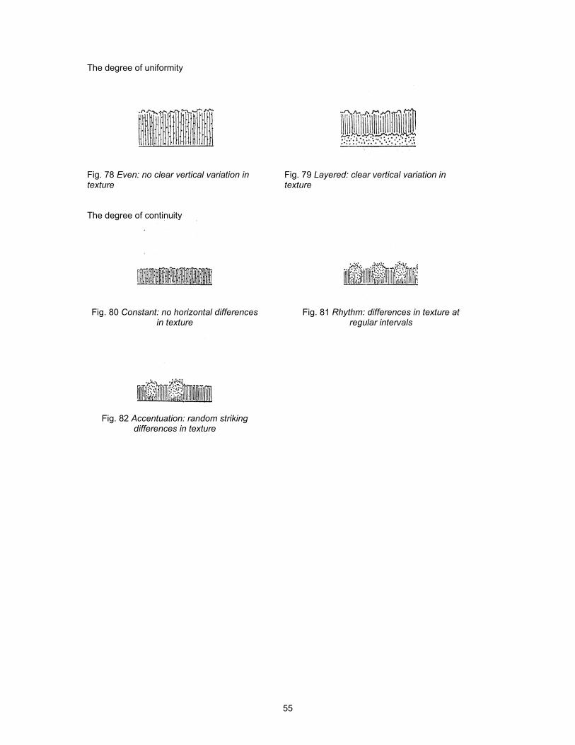
55

The degree of uniformity

Fig. 78 Even: no clear vertical variation in texture

Fig. 79 Layered: clear vertical variation in texture

The degree of continuity

Fig. 80 Constant: no horizontal differences

in texture Fig. 81 Rhythm: differences in texture at

regular intervals

Fig. 82 Accentuation: random striking differences in texture

56

Edge profile

Fig. 83 Receding Fig. 84 Upright

Fig. 85 Overhanging

Degree of naturalness

Fig. 86 Straight and ‘hard’: the planting has

straight contours and ‘hard’ boundaries Fig. 87 Ragged and ‘soft’: the planting has

irregular contours and vague edges

57

Structure

Fig. 88 Trees Fig. 89 Trees with occasional shrubs

Fig. 90 Shrubs with occasional trees

Fig. 91 Shrubs Fig. 92 Trees with a shrub

marginFig. 93 Trees with a shrub

layer

Design tools Each of the characteristic forms described above can be created using different design tools:

Edge

Native stock trimmed to form a hedge

Low-growing non-native plants

Articulation

Native stock trimmed to form a hedge

Smaller, non-native shrubs

Partition

Native shrubs with or without trimmed edges

Larger non-native shrubs

Screening

Tree planting, no crown raising

Tree planting with shrub layer; the trees and shrubs must intertwine

Wall

Native species with a dense, compact habit

Non-native evergreen species

Wide spacing and sufficient thinning to allow full growth and the development of complete foliage cover

No crown thinning, branch reduction or crown raising

Broad plant bed

Curtain

Species with an open and loose habit

Small distances between plants, which encourages them to grow upwards

Crown thinning, branch reduction and crown raising is possible

Narrow plant bed

Window

Native shrubs pruned to the right height

58

Low, non-native shrubs

Widely spaced shrubs for full growth and good foliage cover

Trees with upright crowns

Trees with raised crowns

Even

Large number of species, individually mixed

Small number of species with very similar textures

One species

Layered

A few layers with very different textures

Each layer consists of one species or a few species with very similar textures

Constant

In species-rich planting the length of the planting element must be many times its height (minimum 100 m)

Rhythm

Striking individual trees or shrubs planted at regular intervals

Accentuation

Striking individual trees or shrubs at irregular intervals

Receding

Free growth along the edge

Shrub margin in front of tree planting

Upright

Use of woodland planting as hedge

Tree planting with low branching crowns

Overhanging

Edge pruning in a margin of trees and shrubs

Crown raising in an margin containing only trees

Straight and hard

Pruning for shape

Straight, clearly defined edges

Rhythmic or striking accentuation along the edge

A sharp silhouette

Layered

Ragged and soft

Vague, ill-defined edges; abundant herbs in the edge

Individual mixing of striking species

Ragged silhouette

The effect over time Planting schemes can be grouped according to the way they develop from the time of planting until they reach full maturity.

The first group consists of planting schemes with a pronounced static character. Stated simply, the effect of such planting schemes changes little over time, they just become higher and fuller. These planting schemes are simple, containing just a few species which each have a clear place and contribute to the overall long-term effect. In contrast, the second group consists of planting schemes with a distinctly dynamic character. A typical example is traditional woodland planting schemes: species-rich, individually mixed planting.

59

The roles of the individual species constantly change, creating a succession of visual effects over time.

The final group of planting schemes are those with a cyclical development. The visual effect is obtained by periodic rigorous pruning back to restore the same visual effect.

Design techniques Each of the planting groups described above can be linked to a number of specific design techniques to choose from.

Static planting

The structure of the planting and the role played by each species in the visual effect is determined beforehand.

The way the visual effect will develop is clear from the start; specific maintenance work will need at certain times to achieve this effect.

When the planting has reached maturity the purpose of maintenance work is to maintain vitality and a tidy appearance.

Radical rejuvenation measures are delayed as long as possible.

The ‘nurse crop’ system cannot be used.a

Use of long-lived species.

Rows of different species. Fig. 94 Static planting technique

Dynamic planting

Indicate the characteristic forms that will determine the appearance of the planting (e.g. transparency)The structure of the planting and the role of each species in creating the visual effect are not fixed in advance. During the growth of the planting there are certain moments when the designer and technical maintenance staff have to decide how the planting scheme will continue to develop. The choice is influenced by the previous visual forms.

The ‘nurse crop’ system can be used.

Plants may be individually mixed.

Species with different life cycles may be mixed together, although this makes maintenance more complex and expensive. The most manageable system is to keep to the life cycle of the main plants.

The plant bed must be at least 50 m wide; any narrower and it is extremely difficult to manage the visual effect. The planting will acquire a ragged appearance with, in places, considerable differences in height, texture and transparency.

Fig. 95 Dynamic planting technique

Cyclical planting

The appearance of the planting is fixed beforehand.

The desired appearance develops too quickly but is repeated; the effect is dominated by periodically cutting back to just above ground level.

The timing of pruning is based on the fastest growers – depending on their rate of growth, once every three to seven years.

The ‘nurse crop’ system cannot be used.

Only species amenable to hard pruning can be used.

a In this system the planting mixture contains a number of species which grow faster than the permanent species. Their function

is to protect the main planting during the initial years of growth and are removed after a number of years (see § 0)

60

A wide range of species can be used because species do not have the chance to suppress other species (see section 0).

Restrictions on the choice of plant material Both the nature of the plant material and the environment in which it is planted impose a number of limitations. If these limitations are not properly taken into account in the design, the desired visual effect will not be achieved.

The range of influential factors can be divided into two groups:

The characteristics of the plant material itself, called ‘iron laws’.

Environmental influences, in this case the urban environment.

Iron laws

IntroductionThe native species available for planting differ widely in two respects:

Light requirement

Rate of growth

These differences drive two processes that are always at work in woodland planting schemes:

The natural process of forming open spaces in woodland

Process of species supressing other species

Because these processes always occur they are often called referred to as ‘iron laws’.

The natural process of forming open spaces in woodland Under natural conditions, herbs are in time overgrown by shrubs, which in turn are eventually shaded out by trees. The planting ‘hollows out’, as it were, from the middle. Eventually, the middle of the planting area will consist mainly of trees; shrubs can maintain themselves only along the edges. What develops is, in effect, a natural woodland profile. This process repeats itself when trees die and fall. In the open spaces where sunlight reaches the ground, herbs spring up again, only to be overgrown by shrubs, etc.

This profile does not develop in artificial urban environments because the plant beds are usually far too narrow. This means that in urban areas ‘woodland planting’ based on this natural process can only contain a segment of the natural profile of the woodland edge. There are a number of possibilities:

Fig. 96 Woodland profile

These are called ‘planting forms’ – in effect, no more than combinations of trees and shrubs derived from the natural woodland edge.

Fig. 97 Planting forms

If the process is not the basis of the design, a further option can be added to the list:

61

In such a planting scheme the process must be continually checked, which requires intensive maintenance. The appearance easily degrades if maintenance work is not carried out on time.

Fig. 98 Tree layer with a shrub layer

Each of the planting forms has specific planting and maintenance requirements. These are listed below.

62

Tree layer

Dimensions:

minimum width of the plant bed: 15 metres

in narrower compartments one or two rows of nursery-grown standard trees

Fig. 99 Tree layer

Tree layer with occasional shrubs

In addition to the recommendations for the tree layer above:

the shrubs must tolerate shade

the trees must cast as little shade as possible

Fig. 100 the tree layer with occasional shrubs

Shrub planting

Giving each shrub less space encourages rapid vertical growth. Constraining horizontal growth, though, usually reduces the robustness of each individual shrub.

Fig. 101 Shrub planting

Shrub planting with occasional trees

the trees should cast little shade

trees should be nursery-grown standards planted at least 20 metres or more apart the shrubs must grow more slowly than the trees

Fig. 102 Shrub planting with occasional trees

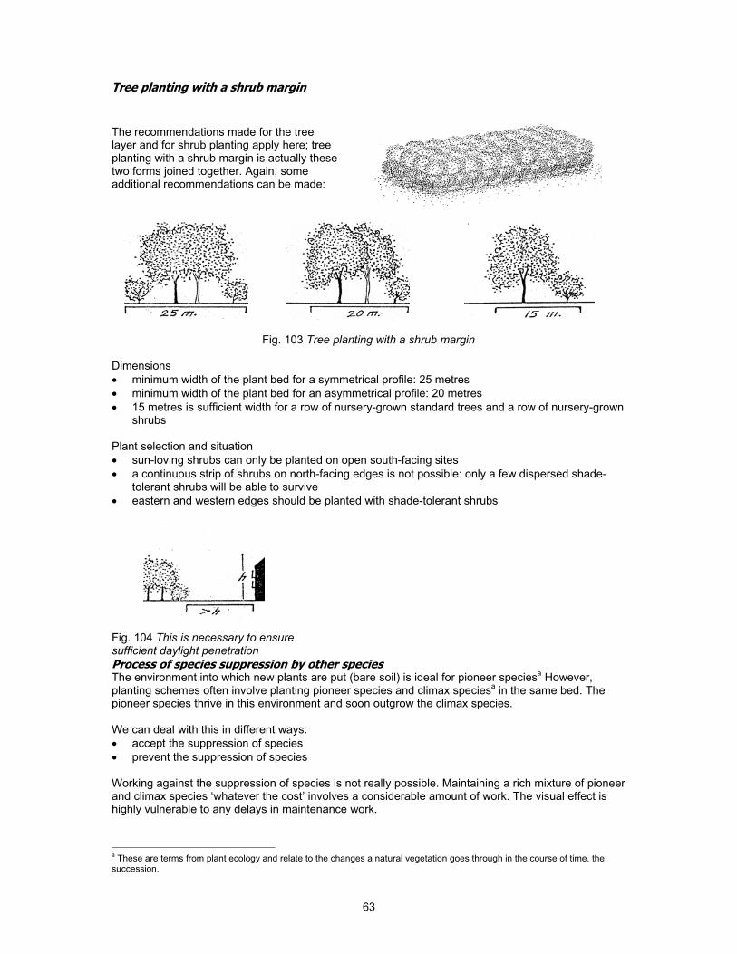
63

Tree planting with a shrub margin

The recommendations made for the tree layer and for shrub planting apply here; tree planting with a shrub margin is actually these two forms joined together. Again, some additional recommendations can be made:

Fig. 103 Tree planting with a shrub margin

Dimensions

minimum width of the plant bed for a symmetrical profile: 25 metres

minimum width of the plant bed for an asymmetrical profile: 20 metres

15 metres is sufficient width for a row of nursery-grown standard trees and a row of nursery-grown shrubs

Plant selection and situation

sun-loving shrubs can only be planted on open south-facing sites

a continuous strip of shrubs on north-facing edges is not possible: only a few dispersed shade-tolerant shrubs will be able to survive

eastern and western edges should be planted with shade-tolerant shrubs

Fig. 104 This is necessary to ensure sufficient daylight penetration

Process of species suppression by other species The environment into which new plants are put (bare soil) is ideal for pioneer species

a However,

planting schemes often involve planting pioneer species and climax speciesa in the same bed. The

pioneer species thrive in this environment and soon outgrow the climax species.

We can deal with this in different ways:

accept the suppression of species

prevent the suppression of species

Working against the suppression of species is not really possible. Maintaining a rich mixture of pioneer and climax species ‘whatever the cost’ involves a considerable amount of work. The visual effect is highly vulnerable to any delays in maintenance work.

a These are terms from plant ecology and relate to the changes a natural vegetation goes through in the course of time, the

succession.

64

Accepting the suppression of species When some slow-growing species have only a temporary role to play in the visual effect, the suppression of species presents no problems. When the planting is still young these species can maintain themselves without difficulty and enhance the appearance of the planting for a while. When the plants grow up they are eventually suppressed and the fast growing species dominate.

This means that:

the appearance of the planting changes quite a lot during its development, in a sequence of intermediary forms

this planting type requires relatively little maintenance

Fig. 105 Intitial species Fig. 106 suppressed later

Preventing the suppression of species If a limited number (1 to 3) of species with the same growth rate are planted none of them will be suppressed. During its development each species plays the same role in the overall effect.

This means that:

the appearance of the planting changes little over time

such planting schemes require relatively little maintenance

Fig. 107 Small number of

speciesFig. 108 not suppressed later

Artificial succession A totally different way of dealing with different growth rates is to use the nurse crop system. Pioneer and climax species are planted together, the pioneers (the nurse crop) protect the climax species when they are young. Once the pioneers have fulfilled their function they are cut, allowing the climax species to develop further.

Fig. 109 Nurse crop Fig. 110 removed Fig. 111 leaves climax species

This approach means:

the appearance of the planting changes considerably and suddenly over time; in effect there are two stages, each with its own appearance

this type of planting requires a relatively high level of maintenance

the appearance degrades if maintenance falls behind schedule

Urban areas

IntroductionBesides the influences of the plants themselves, the influences of the physical environment surrounding the planting also play a role: in this case, the urban environment.

Data on a number of these factors are available, for example on:

65

the soil (profile, mineral composition, organic matter content)

water management regime

traffic engineering requirements (sightlines)

mains services, cables and pipes

building control (distance to outer wall)

pollution (exhaust gases, road salt)

gusts and downdraughts

A few important aspects are discussed below. These are:

the limited space

the limited amount of daylight

informal use (wear and tear)

Limited space It is only really the width of a plant bed that sets firm limitations on the use of woodland planting in urban areas. The plots in urban areas are often too narrow. Native species in particular need plenty of horizontal space to grow freely. Shrubs can easily achieve a diameter of 5 meters and the crowns of the biggest trees can be as much as 10 metres across or more, given time.

The minimum width of a pant bed must be greater than the width of a spreading shrub because after woodland planting has been thinned the margin will never consist of a straight row of plants.

Minimum width of the plant bed

Shrubs in woodland planting require a plot at least 6 metres wide.

A woodland planting that includes trees requires a plot at least 15 metres wide. Plant beds narrower than 6 metres wide

Only suitable for woodland planting if at a later stage the margins are continually cut back or pruned.

Straight row of nursery-grown shrubs or trees.

The required width can then be reduced to 5 metres. If the margins are also cut back the plot may be even narrower.

Non-native species with a narrower growth form.

Fig. 112 Plant beds narrower than 6 metres wide

Besides a sufficiently wide plant bed, a generous margin is needed if plants are to grow freely and reach their full width.

Edges On edges you should leave space for later development.

66

Fig. 113 Leaving space Fig. 114 for later

Another possibility is to plant up the whole plot and remove the outside row at the first thinning.

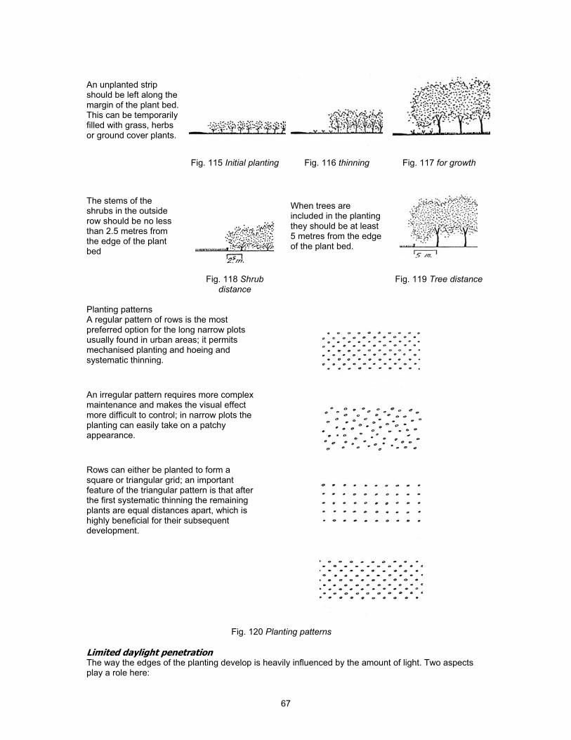
67

An unplanted strip should be left along the margin of the plant bed. This can be temporarily filled with grass, herbs or ground cover plants.

Fig. 115 Initial planting Fig. 116 thinning Fig. 117 for growth

The stems of the shrubs in the outside row should be no less than 2.5 metres from the edge of the plant bed

When trees are included in the planting they should be at least 5 metres from the edge of the plant bed.

Fig. 118 Shrub

distance Fig. 119 Tree distance

Planting patterns A regular pattern of rows is the most preferred option for the long narrow plots usually found in urban areas; it permits mechanised planting and hoeing and systematic thinning.

An irregular pattern requires more complex maintenance and makes the visual effect more difficult to control; in narrow plots the planting can easily take on a patchy appearance.

Rows can either be planted to form a square or triangular grid; an important feature of the triangular pattern is that after the first systematic thinning the remaining plants are equal distances apart, which is highly beneficial for their subsequent development.

Fig. 120 Planting patterns

Limited daylight penetration The way the edges of the planting develop is heavily influenced by the amount of light. Two aspects play a role here:

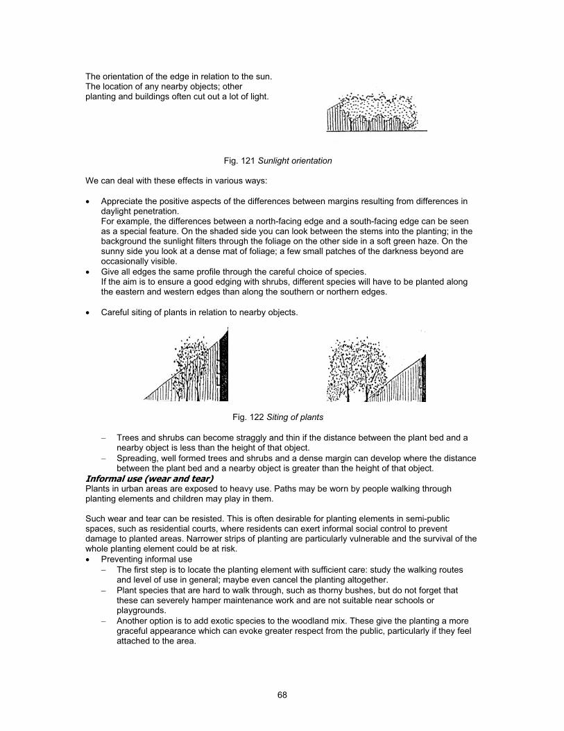
68

The orientation of the edge in relation to the sun. The location of any nearby objects; other planting and buildings often cut out a lot of light.

Fig. 121 Sunlight orientation

We can deal with these effects in various ways:

Appreciate the positive aspects of the differences between margins resulting from differences in daylight penetration. For example, the differences between a north-facing edge and a south-facing edge can be seen as a special feature. On the shaded side you can look between the stems into the planting; in the background the sunlight filters through the foliage on the other side in a soft green haze. On the sunny side you look at a dense mat of foliage; a few small patches of the darkness beyond are occasionally visible.

Give all edges the same profile through the careful choice of species. If the aim is to ensure a good edging with shrubs, different species will have to be planted along the eastern and western edges than along the southern or northern edges.

Careful siting of plants in relation to nearby objects.

Fig. 122 Siting of plants

Trees and shrubs can become straggly and thin if the distance between the plant bed and a nearby object is less than the height of that object.

Spreading, well formed trees and shrubs and a dense margin can develop where the distance between the plant bed and a nearby object is greater than the height of that object.

Informal use (wear and tear) Plants in urban areas are exposed to heavy use. Paths may be worn by people walking through planting elements and children may play in them.

Such wear and tear can be resisted. This is often desirable for planting elements in semi-public spaces, such as residential courts, where residents can exert informal social control to prevent damage to planted areas. Narrower strips of planting are particularly vulnerable and the survival of the whole planting element could be at risk.

Preventing informal use

The first step is to locate the planting element with sufficient care: study the walking routes and level of use in general; maybe even cancel the planting altogether.

Plant species that are hard to walk through, such as thorny bushes, but do not forget that these can severely hamper maintenance work and are not suitable near schools or playgrounds.

Another option is to add exotic species to the woodland mix. These give the planting a more graceful appearance which can evoke greater respect from the public, particularly if they feel attached to the area.

69

Instead of preventing informal use there may be opportunities to make use of it. This may be possible in planting with a clear public function in a more anonymous location. In such places, informal use of planting elements can enrich the functional value of the public domain. Moreover, planting areas in public spaces are usually larger and so informal use is no threat to the survival of the planting element as a whole. Plots accessible to the public must be at least 25 to 30 metres wide (deep).

Accepting informal use

When managing a fait accompli, e.g. surfacing a short cut worn through regular use, the special qualities (e.g. a certain sense of secrecy) of cutting through the vegetation is destroyed.

Not replanting open spots in the planting.

Use species that are resilient to wear and tear.

Opportunities can be created, for example by tipping a pile of sand in the planting area so that children can make a mountain bike arena.

1.4.2 Planting and Habitat

FactorsThe suitability of planting depends on climatological conditions (wind, light, seasons) and physical conditions (soil, groundwater level, air and the space available above and below ground). A different selection of plants is needed behind the dunes along the coast than on a site in a fenland polder or on the sandy soils of Noord-Brabant. As a designer, you will at first be tempted to base your choice of plants on spatial qualities to do with dimension, form (habit), colour and structure. A further consideration is whether the site is in a rural or an urban environment, where there are special restrictions.

Whatever the scale at which you are working, the final detailing is crucial. Financial resources will often be an important consideration (particularly if planting or transplanting older trees is involved).

Climatological conditions WindWind, usually from the sea, is an important factor in the west and north of the Netherlands; frost in the east and south. The effects of wind must be fully considered as it exerts considerable pressure on twigs and branches (in leaf). In rural areas, the direction of the prevailing wind can often be read from the shape of the trees.

Poplars grow rapidly and quickly make a spatial impact, but are ‘not solid enough’. At about 40, branches tend to split and so many trees are felled at around this age. Poplars are not the trees to plant if you want them to be around in 100 years time, although they can live for a long time. As solitaires, it may be worth the extra work, but not for an avenue.

Unfortunately, many a good tree succumbs to our autumn storms; the poorest specimens have by then lost their leaves, but those that still have a good leaf cover are exposed to the full force of the wind.

But wind is not restricted to rural areas. The taller buildings built in recent years create considerable ‘downdraughts’. In front of the Robeco building in Rotterdam some trees have been planted to absorb these downward gusts so that passing cyclists are not literally blown through the air! Climatological conditions, therefore, do play a role in urban planting.

LightLight pollution (albeit only at high levels) and salt (road salting in winter, fish stalls on the market) are disastrous for trees. Light requirement and ‘drip damage’ are more important factors affecting shrubs, and trees with dense crowns permit only a very little undergrowth. The so-called ‘woodland planting’ (plots with trees and shrubs) dating from the 1970s often cause problems now. The trees are large and the undergrowth is dying off purely due to insufficient light. Of the original large plots full of trees and shrubs, only the edges will eventually remain, the planting being hollow under the tree canopy in the middle. If you want the shrubs top remain, plant the trees far apart or choose trees with open crowns that let a lot of light through. ‘Drip damage’ can be a significant problem; some hedges (e.g. Yew) are very susceptible to drip damage, other, like Beech or Sycamore, are unaffected.

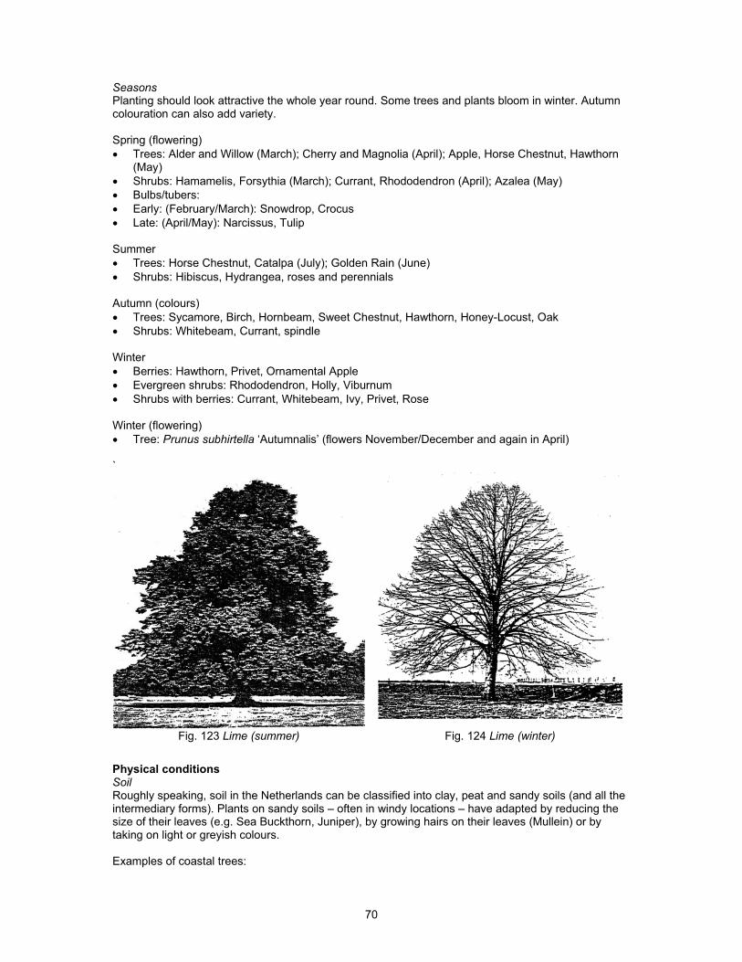
70

Seasons Planting should look attractive the whole year round. Some trees and plants bloom in winter. Autumn colouration can also add variety.

Spring (flowering)

Trees: Alder and Willow (March); Cherry and Magnolia (April); Apple, Horse Chestnut, Hawthorn (May)

Shrubs: Hamamelis, Forsythia (March); Currant, Rhododendron (April); Azalea (May)

Bulbs/tubers:

Early: (February/March): Snowdrop, Crocus

Late: (April/May): Narcissus, Tulip

Summer

Trees: Horse Chestnut, Catalpa (July); Golden Rain (June)

Shrubs: Hibiscus, Hydrangea, roses and perennials

Autumn (colours)

Trees: Sycamore, Birch, Hornbeam, Sweet Chestnut, Hawthorn, Honey-Locust, Oak

Shrubs: Whitebeam, Currant, spindle

Winter

Berries: Hawthorn, Privet, Ornamental Apple

Evergreen shrubs: Rhododendron, Holly, Viburnum

Shrubs with berries: Currant, Whitebeam, Ivy, Privet, Rose

Winter (flowering)

Tree: Prunus subhirtella ‘Autumnalis’ (flowers November/December and again in April)

`

Fig. 123 Lime (summer) Fig. 124 Lime (winter)

Physical conditions Soil Roughly speaking, soil in the Netherlands can be classified into clay, peat and sandy soils (and all the intermediary forms). Plants on sandy soils – often in windy locations – have adapted by reducing the size of their leaves (e.g. Sea Buckthorn, Juniper), by growing hairs on their leaves (Mullein) or by taking on light or greyish colours.

Examples of coastal trees:

71

Alder

Poplar

Oak

Willow

Rowan

Because of their structure, clay and loamy soils retain water for a long time. They are often cold in spring, and less oxygen is available than in sandy soils.

Examples of trees on clay/loam soils

Alder

Horse Chestnut

Birch

Cherry

Another important factor is the presence of calcium, which supports a different type of vegetation; a base-poor dune vegetation contains different plants to calcareous dune valley vegetation. Peaty areas are acid and always moist; nutrient levels are a crucial factor. Alder and Rowan do well in nutrient-rich peat, Birch in nutrient-poor peat. Well-known shrubs suitable for acid soils are Rhododendron and Azalea. If they are planted in other soil types, peat will always have to be added to the soil.

The above also applies, in principle, in rural areas, where plants still have a ‘feel’ for the soil. Clearly, in purely urban environments the original soil is less important for plants, particularly trees.

Sea clay River clay

Peat Sandy soils Loamy soils

Fig. 125 Soils of The Netherlands

Groundwater

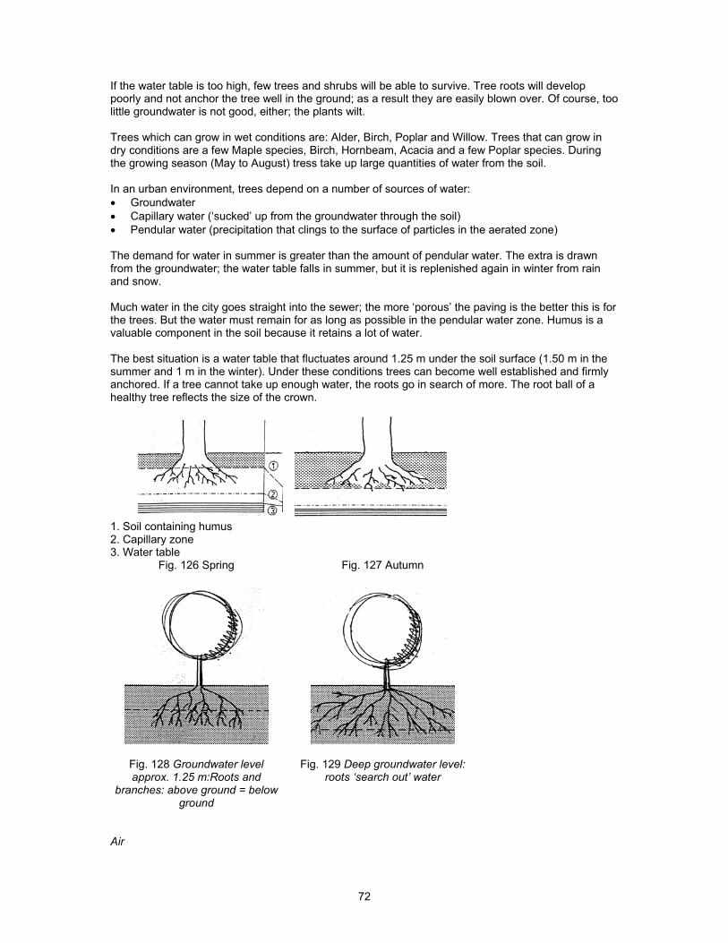
72

If the water table is too high, few trees and shrubs will be able to survive. Tree roots will develop poorly and not anchor the tree well in the ground; as a result they are easily blown over. Of course, too little groundwater is not good, either; the plants wilt.

Trees which can grow in wet conditions are: Alder, Birch, Poplar and Willow. Trees that can grow in dry conditions are a few Maple species, Birch, Hornbeam, Acacia and a few Poplar species. During the growing season (May to August) tress take up large quantities of water from the soil.

In an urban environment, trees depend on a number of sources of water:

Groundwater

Capillary water (‘sucked’ up from the groundwater through the soil)

Pendular water (precipitation that clings to the surface of particles in the aerated zone)

The demand for water in summer is greater than the amount of pendular water. The extra is drawn from the groundwater; the water table falls in summer, but it is replenished again in winter from rain and snow.

Much water in the city goes straight into the sewer; the more ‘porous’ the paving is the better this is for the trees. But the water must remain for as long as possible in the pendular water zone. Humus is a valuable component in the soil because it retains a lot of water.

The best situation is a water table that fluctuates around 1.25 m under the soil surface (1.50 m in the summer and 1 m in the winter). Under these conditions trees can become well established and firmly anchored. If a tree cannot take up enough water, the roots go in search of more. The root ball of a healthy tree reflects the size of the crown.

1. Soil containing humus 2. Capillary zone 3. Water table

Fig. 126 Spring Fig. 127 Autumn

Fig. 128 Groundwater level approx. 1.25 m:Roots and

branches: above ground = below ground

Fig. 129 Deep groundwater level: roots ‘search out’ water

Air

73

Trees in built-up areas – except trees in parks and gardens – grow in a habitat that simply cannot be compared with a site in a wood or open landscape. The soil in the country is open (to air and water) and fallen leaves provide a supply of nutrients. Conditions in urban areas are very different. Paving requires well compacted soil; but trees need open soils. Air is kept out by the closed road surface and compacted soil, which leaves almost no pore volume for air to penetrate.

In open soils, about 50% of the volume is air; below 15% oxygen, roots become stunted, at 11% oxygen they start to die. All paving seals the surface of the soil and so open spaces – slotted flags or widely spaced paving bricks – are essential. Trees cannot develop roots under asphalt surfaces (0% oxygen). The pressure and vibration caused by heavy traffic further compacts the soil.

In ‘sinking’ areas (peat soils) in the West of the Netherlands the paving has to be raised every so often, even up to 30 or more centimetres at a time. As a result, many trees receive too little oxygen and die. Oak and Beech always die, Lime trees grow a new layer of roots if the additional soil layer is no deeper than 25 to 30 cm. Elms and Planes tolerate these conditions quite well.

A. Sinkhole B. Sawn kerb, min. length 500 C. Kerb type Cru 80 D. Tree grille Cruquius concrete blue limestone colour 1200 x 1200 x 120 E. Air grate F. Dark paving brick (size, 20x6.6x6) G. Dark paving brick (Waal size, 20x5x7)

`

Fig. 130 Tree pit

Root corridor and tree pit Urban trees cannot be viewed in isolation from their environment; they are one of the factors that define the public domain in the city. Street trees add to the quality of public spaces and have a different effect in each place. When planting trees in urban areas it is wise to design a strip for trees only, with no cars, cables and pipes or street furniture: a ‘corridor’. This ‘plantpit’ can be finished with a 10 cm layer of sand, with paving on top (with no risk that the paving will sink any faster than the surrounding area).

If this is not possible, a tree pit of 2 x 2 x 1 m should be made and filled with suitable tree soil. Tree soil is light soil, contains approx. 4% humus, is well aerated and well drained, retains water well and contains sufficient nutrients. Where more air is required in the soil, perforated drainage pipes can be used as ‘air pipes’ to ensure better aeration of the soil.

In many places, though, hard road surfacing and numerous mains services and cables leave no room for planting. In these situations the minimum area required for a tree is 7.5 m on both sides (i.e. 15 m apart) because otherwise they will have an even greater struggle for survival. The more open the structure of the topsoil, the better this is for the tree.

It is important to choose a good tree grille. Square tree grilles are often used in paved areas because these fit well into the pattern of most paving materials. Cast iron or metal tree grilles are attractive, but

74

expensive. Accumulation of dirt and rubbish in the space between the grille and the soil (approx. 10 cm) can be prevented by filling this space with Argex pellets until right under the grille. These are light, expanded clay granules (reddish brown) which considerably improve aeration. Another attractive solution is to use gravel. A cheaper option is 30 x 30 cm slotted flags. In parking areas always ensure that the tree trunk is protected.

Cross-section Pavement Tree corridor Road / main sewer Pavement / cables and pipes

Fig. 131 Cross-section

Types of trees Size, form, structure, colour Size and form not only depend on climatological and physical factors, but also have a major impact on the streetscape. In spatial terms, they may or may not provide structure or accentuate the spatial composition (see Tree Structure Plan Amsterdam). Texture relates to the shape, size and arrangement of the leaves and it is very important when detailing to ensure compatibility with the materials used. Colour speaks for itself. A significant fact is that light green tints have the effect of expanding spaces, dark green and red-brown make spaces seem smaller and can create a sombre atmosphere. Copper-leaved trees are striking, particularly as solitaires, such as Copper Beeches on farms (also Sycamore/Maple, Apple, Cherry, Oak).

Choosing a tree When choosing trees, consider the amount of space above ground. If you meet the conditions discussed above (tree pit, soil, etc.) there is a chance that the trees will grow to maturity and attain their full size. Plane trees can easily have branches 10 m long, and so they should be planted 12 m from buildings. If the pavement is not very wide, choose a tree a size or two smaller or a tree with a columnar crown. If not, the crown will soon grow up against wall and must either be pruned each year, or the tree felled and another species planted.

Size classes of trees

Size class 1: 15 m and taller

Size class 2: to about 10 m

Size class 3: to about 5 m

Size 1 trees develop crowns at least 15 metres across. Large dense crowns must be avoided in small streets, where trees with light open crowns are to be preferred (e.g. Gleditsia/Honey Locust). For most residents the minimum acceptable distance between crown and wall is about 2 metres. Obviously, planting distances will bear some relation to the location of the doorways, drives and passages along street frontages.

Planting distances If trees are planted very close to buildings, drastic measures are repeatedly needed to ensure enough daylight penetration. Sometimes these measures can be so drastic that the resulting remnant of the tree may no longer make a positive contribution to the streetscape.

To plant trees that can develop freely with the minimum number of complaints, you need to weigh up the following considerations:

The nature of the building facade

The distance between the trees and the building

The distance between the trees

75

The tree species

The pruning method

In real terms, this means that when planting new trees, minimum distances must be adhered to. Greater distances should be used when planting trees with a broad, dense crown, such as Plane and Horse Chestnut.

Trees may only be planted at shorter distances than given in the table:

When planting trees with a columnar or thin crown

Along ‘blind’ walls

When special pruning methods are used, such as espalier, pyramid pruning and pollarding

When only a few trees are planted along a street frontage

Rows of trees let through very different amounts of daylight, depending on whether the crowns of the trees join together (closed) or are spaced apart. This makes it important to note the relevant planting distances for the various size classes.

1.1.1.1.1.1 Planting As a rule trees are planted between 1 November and 15 April. They are then resting and have the best chance of becoming established.

Standard sizes of trees for planting are:

14–16 cm girth (approx. 5 cm diameter)

16–18 cm girth (approx. 6 cm diameter)

18–20 cm girth (approx. 6.5 cm diameter) The price ratio for these sizes is 1:1.5:2.

Planting distances for rows of trees:

Size class open row (spaces between crowns)

closed row (crowns touching)

size class 1 > 18 m 5–10 m size class 2 > 12 m 5–8 m size class 3 > 9 m < 5 m

Minimum distance between the buildings and the centre of the stem

size class min. distance stem to building size class 1 6 m size class 2 4 m size class 3 3 m

In urban renewal areas where high levels of vandalism are expected it is better to plant fewer larger trees rather than a larger number of thinner trees.

Transplanting Trees with stems about 30 cm diameter can be transplanted; the larger the tree, the more expensive the operation. Trees with bigger stems can be transplanted, but their chances of survival are much smaller. Ensure that the root ball is as large as possible (min. 3 m across and 1–1.5 m deep). If you know well in advance that a tree will be transplanted the roots can be cut when the tree is still standing, and new hair roots will grow to form a neat compact root ball. This can be done is summer or winter. The latest method is to soak the root ball in winter. This then freezes to create a solid ball of soil and roots. The tree can then be lifted out with a crane and transported by trailer to its new site. After planting (good pit and tree soil, etc.) the tree should be pruned to restore the balance between the root system and the crown. Prices depend on size, transport options (disconnecting the overhead tram lines, transplanting at night, etc.) and financing. Transporting a Horse Chestnut with a stem diameter of 45 cm over a distance of 1 km (difficult journey, disconnection of tramlines and transport by night) costs about € 10,000 per tree.

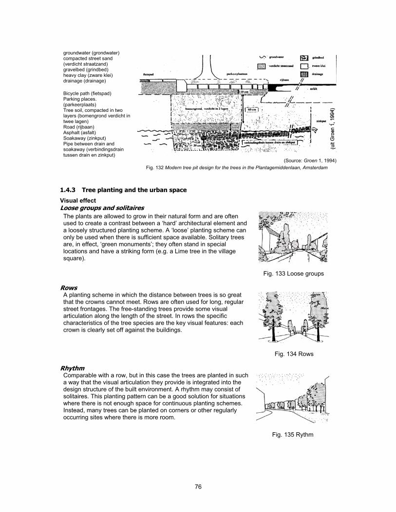
76

groundwater (grondwater) compacted street sand (verdicht straatzand) gravelbed (grindbed) heavy clay (zware klei) drainage (drainage)

Bicycle path (fietspad) Parking places. (parkeerplaats) Tree soil, compacted in two layers (bomengrond verdicht in twee lagen) Road (rijbaan) Asphalt (asfalt) Soakaway (zinkput) Pipe between drain and soakaway (verbindingsdrain tussen drain en zinkput)

(Source: Groen 1, 1994)

Fig. 132 Modern tree pit design for the trees in the Plantagemiddenlaan, Amsterdam

1.4.3 Tree planting and the urban space

Visual effect

Loose groups and solitaires

The plants are allowed to grow in their natural form and are often used to create a contrast between a ‘hard’ architectural element and a loosely structured planting scheme. A ‘loose’ planting scheme can only be used when there is sufficient space available. Solitary trees are, in effect, ‘green monuments’; they often stand in special locations and have a striking form (e.g. a Lime tree in the village square).

Fig. 133 Loose groups

RowsA planting scheme in which the distance between trees is so great that the crowns cannot meet. Rows are often used for long, regular street frontages. The free-standing trees provide some visual articulation along the length of the street. In rows the specific characteristics of the tree species are the key visual features: each crown is clearly set off against the buildings.

Fig. 134 Rows

RhythmComparable with a row, but in this case the trees are planted in such a way that the visual articulation they provide is integrated into the design structure of the built environment. A rhythm may consist of solitaires. This planting pattern can be a good solution for situations where there is not enough space for continuous planting schemes. Instead, many trees can be planted on corners or other regularly occurring sites where there is more room.

Fig. 135 Rythm

77

Screen A screen is a transparent wall of trees through which the facades of the buildings are more or less visible, depending on the viewpoint. A screen is best created using species with an open crown in which the branches do not grow in one main direction so that they easily flow together to form a visual whole. Elms are good trees for creating a screen. Some other species, if planted close together and with some extra pruning, can also be used to create a screen effect. A problem, though, is that if the trees are planted close together the transparent effect can easily be lost.

Fig. 136 Screen

WallA wall consists of multiple rows of trees planted short distances apart so that the crowns grow into each other. If tree species that develop dense crowns are used (e.g. Lime) it may even be possible to plant just one row; the trees must then be no more than 8 m apart. In the summer this planting scheme creates the effect of a ‘green wall’. It is important that the trees form a continuous whole. If the planting distances are too great or if too many trees are missing from the row, the wall effect is largely lost.

Fig. 137 Wall

Canopy

A canopy consists of multiple rows of trees short distances apart and with intertwining crowns. The most suitable trees species are those with a broad, fairly open crown. The canopy effect is largely lost if the trees are planted too far apart to form a unified mass.

Fig. 138 Canpy

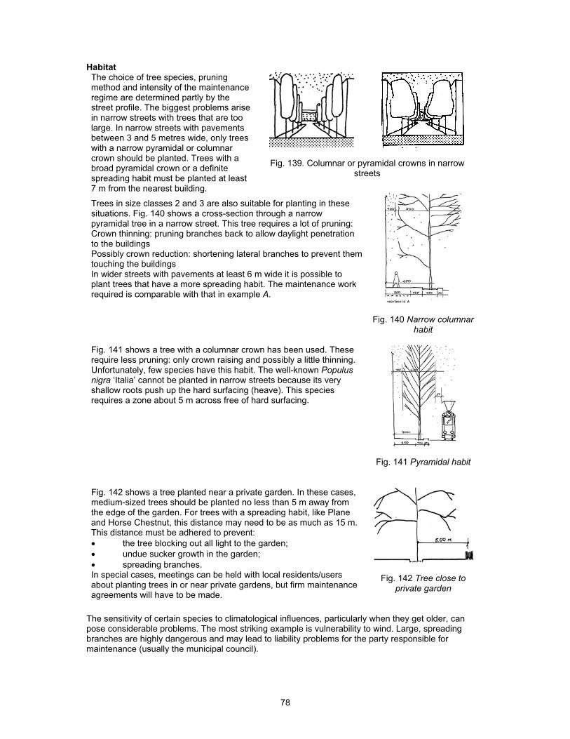
78

Habitat

Fig. 139. Columnar or pyramidal crowns in narrow streets

The choice of tree species, pruning method and intensity of the maintenance regime are determined partly by the street profile. The biggest problems arise in narrow streets with trees that are too large. In narrow streets with pavements between 3 and 5 metres wide, only trees with a narrow pyramidal or columnar crown should be planted. Trees with a broad pyramidal crown or a definite spreading habit must be planted at least 7 m from the nearest building.

Trees in size classes 2 and 3 are also suitable for planting in these situations. Fig. 140 shows a cross-section through a narrow pyramidal tree in a narrow street. This tree requires a lot of pruning: Crown thinning: pruning branches back to allow daylight penetration to the buildings Possibly crown reduction: shortening lateral branches to prevent them touching the buildings In wider streets with pavements at least 6 m wide it is possible to plant trees that have a more spreading habit. The maintenance work required is comparable with that in example A.

Fig. 140 Narrow columnar habit

Fig. 141 shows a tree with a columnar crown has been used. These require less pruning: only crown raising and possibly a little thinning. Unfortunately, few species have this habit. The well-known Populus nigra ‘Italia’ cannot be planted in narrow streets because its very shallow roots push up the hard surfacing (heave). This species requires a zone about 5 m across free of hard surfacing.

Fig. 141 Pyramidal habit

Fig. 142 Tree close to private garden

Fig. 142 shows a tree planted near a private garden. In these cases, medium-sized trees should be planted no less than 5 m away from the edge of the garden. For trees with a spreading habit, like Plane and Horse Chestnut, this distance may need to be as much as 15 m. This distance must be adhered to prevent:

the tree blocking out all light to the garden;

undue sucker growth in the garden;

spreading branches. In special cases, meetings can be held with local residents/users about planting trees in or near private gardens, but firm maintenance agreements will have to be made.

The sensitivity of certain species to climatological influences, particularly when they get older, can pose considerable problems. The most striking example is vulnerability to wind. Large, spreading branches are highly dangerous and may lead to liability problems for the party responsible for maintenance (usually the municipal council).

79

Achieving the desired visual effect Besides the habitat of the trees, other essential factors in achieving the desired visual effect are the choice of species and planting scheme. If, for example, a screen of trees is to be planted in a street, the designer will have to decide whether to use a slow-growing species at short distances apart or a fast-growing species planted further apart. In narrow streets, however, fast-growing species will soon cause problems and it is better not to use them.

There are three methods for achieving a reasonably good planting(visual effect(time)) in a relatively short time:

plant slower growing trees at short intervals;

plant a mix of fast and slow growing species;

plant semi-mature trees (more than 10 years old).

Re 1: Planting at short intervals quickly yields a reasonably good visual effect. Short distances between trees are often necessary to obtain a screen or wall effect. An advantage of planting trees close together is that the trees compete for light and quickly grow upwards, giving an upright habit with straight stems. A disadvantage is the extra pruning that is often required.

Re 2: Mixing species with different growth rates requires intensive maintenance work which must be carried out promptly. It is only recommended for planting in broad strips of vegetation (woodland planting). The advantage here is that slow growers are ‘forced up’ by faster growing species. This only works with some species: Elms can be combined with Poplars; Oaks grow too slowly and are eventually shaded out.

Re 3: Another option is to plant semi-mature trees at their final distances apart. Semi-mature trees, however, find it hard to adapt to their new habitat and it takes a few years before they grow at their normal rate again. Moreover, transplanting is an expensive business. An advantage of container trees is that they can be planted easily and successfully at any time, even outside the planting season. This makes these trees highly suitable for use in special situations: rapid restoration of planting schemes in squares or along an important road, or after accidents, etc. However, container trees are often slow to become established and can be ‘overtaken’ by smaller, root-balled trees.

Planting distances When deciding on the planting distances needed to achieve the desired visual effect the following points should be considered:

the final diameter of the crown of the tree

height of the tree

the habit of the tree (tree shape, height/width ratio, openness of the crown)

the root system

shading of nearby buildings

width of the road and path (for canopy effect)

the relation between the final height of the tree and nearby buildings

the period needed to achieve the desired visual effect A number of examples are presented to explain points 1, 2 and 3.

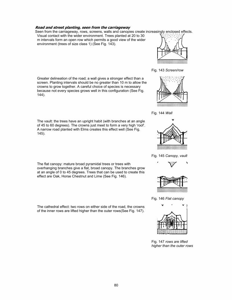
80

Road and street planting, seen from the carriageway Seen from the carriageway, rows, screens, walls and canopies create increasingly enclosed effects. Visual contact with the wider environment. Trees planted at 20 to 30 m intervals form an open row which permits a good view of the wider environment (trees of size class 1) (See Fig. 143).

Fig. 143 Screen/row

Greater delineation of the road; a wall gives a stronger effect than a screen. Planting intervals should be no greater than 10 m to allow the crowns to grow together. A careful choice of species is necessary because not every species grows well in this configuration (See Fig. 144).

Fig. 144 Wall

The vault: the trees have an upright habit (with branches at an angle of 45 to 60 degrees). The crowns just meet to form a very high ‘roof’. A narrow road planted with Elms creates this effect well (See Fig. 145).

Fig. 145 Canopy, vault

The flat canopy: mature broad pyramidal trees or trees with overhanging branches give a flat, broad canopy. The branches grow at an angle of 0 to 45 degrees. Trees that can be used to create this effect are Oak, Horse Chestnut and Lime (See Fig. 146).

Fig. 146 Flat canopy

The cathedral effect: two rows on either side of the road, the crowns of the inner rows are lifted higher than the outer rows(See Fig. 147).

Fig. 147 rows are lifted higher than the outer rows

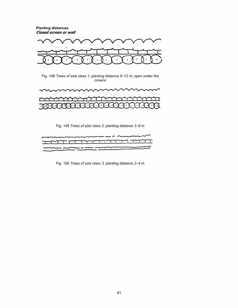
81

Planting distances

Closed screen or wall

Fig. 148 Trees of size class 1; planting distance 5–12 m; open under the crowns

Fig. 149 Trees of size class 2; planting distance 3–8 m


82

Row

)Fig. 151 Trees of size class 1; planting distance 20–30 m



83

Silhouettes of the different trees

Fig. 154 Alder (els) Fig. 155 Black Poplar (populier)

Fig. 156 Ash (es) Fig. 157 London Plane (plataan)

Fig. 158 Elm (iep) Fig. 159 Common Oak / Pedunculate Oak (eik)

Fig. 160 Downy/White Birch (witte berk)

Fig. 161 Sycamore / Great Maple (esdoorn)

Fig. 162 Locust Tree / False Acacia (acacia)

Fig. 163 Common Lime (linde)

Fig. 164 Common Beech (beuk)

Fig. 165 Horse Chestnut (kastanje)

Fig. 166 Weeping Willow (treurwilg)

Fig. 167 White Willow (schietwilg)

Fig. 168 Pollarded Willow (knotwilg)

Fig. 169 Weeping Ash (treures)

Pruning There is a balance between the amount of leaves and roots a tree has. If too much growth (above ground) is cut away the tree will compensate for its shortage of leaves by throwing up many new shoots. Pollarded trees such as Poplar and Willow must be pruned each year. Trained trees/espaliers are grown for their architectural form. Examples are:

Lime

Plane

Hornbeam

84

A nursery grown tree has been pruned in the nursery to obtain a clear stem height of 2 m while its natural form is maintined. During the first 5 to 10 years the crown of the tree will require some light pruning. Trees close to the edges of a road must have their lower branches remove to ensure sufficient clearance for passing traffic.

Trees do not last forever, so do not hesitate to remove old specimens with a limited life expectancy and plant younger trees!

Crown raising Trees planted along roads and paths should have their lower branches removed. This crown raising (to a height of about 2.5 m) is started when the trees are still young. Depending on the situation, a street tree will have to undergo further crown raising over the years. In some cases up to as much as 7 m above ground level (species with hanging branches).

When raising a tree crown thought should be given to obtaining the right balance between the length of the stem and the crown (2:3 or 1:2). It is an unattractive sight for a tree of 14 m to have a clear stem height of 7 m. In these cases it is better to go for an asymmetrical crown. In the example above the tree may have its crown raised to 4 m on the pavement side, but up to 7 m. on the side above the road. This gives the streetscape a much better appearance. The rows of Elms planted along canals are a good example of asymmetrical crown raising. In some cases, pruning will still be necessary on the side facing the buildings to ensure sufficient daylight penetration.

Fig. 170 crown raising near

building

Fig. 171 crown raising along a

canal

Fig. 172 partial crown lifting

Fig. 173 crown raising in grass

Fig. 174 crown raising in a street

Crown raising heights

85

planting stock 2.5 m residential streets 3 m main roads 4.5 m tram lanes 4.5 m trees with hanging branches to 7 m asymmetrical: housing side asymmetrical: canal + quayside asymmetrical: canal + grass

2.5 m 2.5 m 0–2.5 m

in grass 0–2.5 m in ground cover 0–2.5 m in low shrubs (to 1.5 m) 0–2.5 m in medium-sized shrubs (to 2 m) 2.5 m in tall shrubs (from 2 m) 2–7 m

Summary The choice of plants depends on: 1. The site and growing conditions 2. Growth characteristics and habit of the planting material 3. The appearance of the planting and the atmosphere it creates 4. Practical aspects (function and goal) 5. Cost and available funds

1. Site and growing conditions

natural landscape

cultivated landscape

urban area

nature and character of the buildings (tall buildings create windy conditions) Growing conditions Soil type Sand nutrient rich Peat nutrient poor Clay calcareous / lime rich non-calcareous / base poor acid good/poor structure humus content Groundwater levels

high – wet

low – dry

water retaining capacity of the soil Climatological conditions

sheltered

exposed

coastal

urban area

industrial site

wind

frost Light requirement

open site / full sun

semi-shade

full shade 2. Growth characteristics and habit Tree dimensions Size class 1 Size class 2 Size class 3 Shrub dimensions Evergreen – taller than 4 m Deciduous 2–4 m 0.5–2 m less than 0.5 m Crown shape and habit of trees

spherical

spreading

broad pyramidal

Texture

leaf shape

leaf size o large o medium o small

leaf arrangementLeaf colour

light green – dark blue-green

light to dark brown

yellow

variegated Blossom

flower colour

flowering season early spring

spring

summer

autumn

fruit

autumn colour

bark 3. AppearanceVisual effect

ankle height

knee height

waist height

breast height

eye level

above eye level Mutual relation between elements

harmony

contrast

rhythm

decorative value

4. Practical aspects

winter hardness

vitality

disease resistance

abundant and/or long-lasting blossom

function in the plan

spatial layout

relation to buildings

relation to existing planting

86

narrow pyramidal

columnar

weeping Crown shape and habit of shrubs

groundcover

spreading

upright

compact

overhanging

client’s wishes

wind protection

shade

traffic guidance

noise reduction

enclosure

ground cover 5. Costs

purchase costs and required dimensions

intensity of maintenance

length of implementation period

available financial resources

1.4.4 Hedges Hedges divide the space where a fence or wall is undesirable. The primary function of a hedge is always separation, most obviously to divide two uses, for example to divide a private space (garden) from the public space. Hedges provide a natural background for other plants; thorny hedges form an impenetrable barrier. Hedges have an important spatial effect. They can be classified into those which divide up the space in which they stand (‘free-standing’) and those that form part of a larger mass immediately behind them.

When the spatial impacts of hedges are examined more closely, it seems obvious to classify them by height. According to their application, we can then distinguish: edges (to approx 0.5 m high), partitions (0.5–1.5 m) and full screens (more than 2 m high). Their respective applications are: as an edge when used to mark out patterns or a composition of lines, as partitions when their function is to resist or direct movement, and as a full screen to visually seal off a space.

One spatial effect of hedges is to facilitate comprehension of the scale of the space and the elements in it, because the hedge has a consistent size (height) which serves as a reference on a human scale. Another spatial effect is created if the hedge is quite long and forms a connecting element that provides continuity. For this purpose hedges do not have to be trimmed; a row of shrubs (a ‘loose hedge’) can also create this effect. Besides their spatial effects, hedges may also, possess a number of intrinsic characteristics.

Natural (loose) habits of shrubs can be tightened up by pruning to form a hedge. These neater forms give hedges a more cultivated appearance, and the hedge is a symbol of continuous human intervention in the natural process of growth. A trimmed hedge can be used in two ways: As a contrast with ‘looser’ forms in the surrounding area, or with a less cultivated environment (e.g. a neat hedge around a farm, set in an agricultural or quasi-natural landscape). As a harmonising element; the regular ‘architectural’ shape of the hedge harmonises with an architectural, usually urban, environment.

Hedges may have an ornamental value, which cannot be seen in isolation from the above – the contribution the hedge makes to the appearance of the wider environment. The characteristics of hedges discussed above make them an ideal means to accentuate a prominent location.

Hedges have two major disadvantages. First, they have to be pruned regularly, in some cases two or three times a year. Second, they take up considerable quantities of nutrients, which are then not available for any plants near the hedge, making regular fertilisation necessary.

Hedges for marking out spaces

Hedges between the main road and bicycle lane or footpath These hedges are planted for traffic safety reasons: they make crossing impossible and at night they prevent glare from the headlights of oncoming traffic. These street profiles are only found in post-war urban areas and non-urban areas. Trimmed hedges require a lot of maintenance, though, and in these situations can easily be replaced by untrimmed hedge/shrub planting if there is sufficient space, or, in places where the safety function is not essential, by a normal verge.

Hedges along watercourses (See Fig. 175)These are also planted for safety reasons, to keep children away from the water. The hedge is a friendlier type of fence. The need for and value of hedges in the neighbourhood should be

87

determined. Such hedges do not remove the danger altogether, but keep it at a distance and make it less threatening, but, because of this very effect, can make the (unknown) danger much greater.

In addition to the functions mentioned above, these uses of hedges can enhance appreciation of the scale of the space in which they stand.

Hedges as a visual screen to hide (mainly) parked cars (See Fig. 178)This use of hedges is particularly dependent on the environment. They are suitable for this purpose in an urban environment, but in other environments they can easily be replaced by an untrimmed hedge or shrubs. It may even be worth considering removing some taller plants; owners often want to see their parked cars from the house.

Hedges as space-shaping elements Hedges can create their own separate (sub)rhythm different in character from the larger space they are part of. An example is a garden surrounded by a hedge, possibly in a park, the regular form providing a contrast that sets off the space. In this case the trimmed hedge is an essential element. Should the situation within the hedges ‘not work’, it is better first to see if another use of the space can improve the situation before deciding to grub up any hedges. Hedges are planted around playgrounds and seating areas mainly for safety reasons because they stop children running onto the road. Besides this strictly functional aspect, hedges also provide ‘shelter’ and ‘security’ for the play area. In other words, the hedge marks out a territory.

The same quality of ‘security’ or ‘cover’ is provided by hedges surrounding a sitting area with benches. A trimmed edge is justified around such areas if they form a contrast with the loose forms in the area and so create their own place, or if the site is located within a paved area where the use of hedges adds an architectural dimension and has a practical effect of saving space (the ‘paved character’ relates to walls as well as horizontal surfaces).

Hedges as edging for a mass

The hedge as linear element A tall or medium-sized hedge can provide a background for roses, for example, or a border. Removing such a hedge often destroys the appearance of the border and is only advisable if the border is of a sufficient size.

Hedges that form a pattern or composition of lines Very low hedges, which are essentially an edging, are found around borders of roses or perennials. Often they are laid to give the border a less dreary look when there is little to see in the border itself. This situation has value only if two conditions are met:

The height of the hedge is in proportion with the planting material in the border The hedges themselves form a particular pattern that is interesting enough when the roses of perennials have been pruned or cut down.

Use of these types of hedge is only justified in prominent places or in situations where there is very little green. Moreover, their maintenance is time-consuming in proportion to their length. Sometimes a compromise solution is acceptable to reduce the length of such hedges.

88

Fig. 175 Hedge along watercourse

Fig. 176 Contrast Fig. 177 Hedge in open space

Fig. 178 Hedge bordering car park

Fig. 179 Harmony Fig. 180 Hedge as part of a mass

Fig. 181 Hedge enclosing a garden

Fig. 182 Partition Fig. 183 Edges

Fig. 184 Hedge round a ‘place’

Fig. 185 Hedge bordering shrub bed

Fig. 186 Complete screen

Fig. 187 Shelter for seating

Fig. 188 Edge Fig. 189 Background to border

Planting distance Loose/regular Growth rate

Evergreen hedges

89

Box (Buxus sempervirens) 5/m1 regular Holly (Ilex aquifolium) 3 à 4/m1 regular Common Yew (Taxus baccata) 3/m1 regular Holly (Ilex aquifolium) loose Privet (Ligustrum ovalifolium)Size 40–60

3 à 4/m1 regular

Deciduous hedges Hornbeam (Carpinus betulus) 4/m1 regular Beech (Fagus silvatica) 3 à 4/m1 regular Hawthorn (Crategus monogyna) loose Blackthorn (Prunus spinose) loose Rose – botanical roses loose Growth rate: number of years until the plant reaches a height of 1.5 metres (depending on habitat, soil type and maintenance)

Pruning hedges

Fig. 190 vertical Fig. 191 rounded Fig. 192 tapered

1'6 )25 '(6,*1 - taekemdejong.nl WIND WATER/SUN blz 8 … · Prof.dr.ir. T. M. de Jong ed....

Documents

Transcript of 1'6 )25 '(6,*1 - taekemdejong.nl WIND WATER/SUN blz 8 … · Prof.dr.ir. T. M. de Jong ed....