
16-10.031 review note wipla GRO - nlog.nl note wipla gro.pdf · interpolation creates a smoother...
51
Princetonlaan 6 3584 CB Utrecht Postbus 80015 3508 TA Utrecht www.tno.nl T +31 88 866 42 56 Date 26 mei 2016 Our reference 16-10.031 Contact Dr. K. van Thienen-Visser E-mail [email protected] Direct dialling +31 88 866 42 65 The General Terms and Conditions for commissions to TNO, as filed with the Registry of the District Court in the Hague and with the Chamber of Commerce and Industry in The Hague, shall apply to all commissions to TNO. Our General Terms and Conditions are also available on our website www.tno.nl. A copy will be sent upon request. Trade register number 27376655. Retouradres: Postbus 80015, 3508 TA Utrecht Onderwerp Review Winningsplan Groningen Op 1 april jl. heeft de NAM u een winningsplan voor het Groningen veld doen toekomen. Het Staatstoezicht op de mijnen heeft TNO gevraagd om een aantal technische aspecten van dit winningsplan nader te bestuderen. De vragen betreffen aspecten van de volgende modellen: statische model, dynamische model, compactiemodel, bodemdalingsmodel en grondbewegingsmodel van het Groningen veld. Daarnaast is gevraagd om de bodemdalingsvoorspellingen te evalueren. De resultaten zijn per onderwerp gepresenteerd in vier aparte notities (A-D), die als appendices aan deze brief zijn toegevoegd. Ter bevordering van deling van de analyse en bevindingen met internationale experts zijn de notities in het Engels geschreven. Hoogachtend, I.C. Kroon Bijlage A Review statische model Bijlage B Review dynamische model Bijlage C Review compactiemodel en bodemdaling Bijlage D Review grondbewegingsmodel Staatstoezicht op de Mijnen T.a.v. de heer H. van der Meijden Postbus 24037 2490 AA DEN HAAG 2490AA24037
Transcript of 16-10.031 review note wipla GRO - nlog.nl note wipla gro.pdf · interpolation creates a smoother...
Princetonlaan 6 3584 CB Utrecht Postbus 80015 3508 TA Utrecht www.tno.nl T +31 88 866 42 56 Date 26 mei 2016 Our reference 16-10.031 Contact Dr. K. van Thienen-Visser E-mail [email protected] Direct dialling +31 88 866 42 65 The General Terms and Conditions for commissions to TNO, as filed with the Registry of the District Court in the Hague and with the Chamber of Commerce and Industry in The Hague, shall apply to all commissions to TNO. Our General Terms and Conditions are also available on our website www.tno.nl. A copy will be sent upon request. Trade register number 27376655.
Retouradres: Postbus 80015, 3508 TA Utrecht
Onderwerp
Review Winningsplan Groningen
Op 1 april jl. heeft de NAM u een winningsplan voor het Groningen veld doen toekomen. Het Staatstoezicht op de mijnen heeft TNO gevraagd om een aantal technische aspecten van dit winningsplan nader te bestuderen. De vragen betreffen aspecten van de volgende modellen: statische model, dynamische model, compactiemodel, bodemdalingsmodel en grondbewegingsmodel van het Groningen veld. Daarnaast is gevraagd om de bodemdalingsvoorspellingen te evalueren. De resultaten zijn per onderwerp gepresenteerd in vier aparte notities (A-D), die als appendices aan deze brief zijn toegevoegd. Ter bevordering van deling van de analyse en bevindingen met internationale experts zijn de notities in het Engels geschreven. Hoogachtend,
I.C. Kroon Bijlage A Review statische model Bijlage B Review dynamische model Bijlage C Review compactiemodel en bodemdaling Bijlage D Review grondbewegingsmodel
Staatstoezicht op de Mijnen T.a.v. de heer H. van der Meijden Postbus 24037 2490 AA DEN HAAG
2490AA24037
Appendix A | 1/16
Date 26 mei 2016 Our reference 16-10.031
A Static model review
The Groningen Field Review 2012 (GFR2012) has been updated by NAM in 2015 (GFR2015). The static reservoir model of the Groningen Field, which is part of the GFR, has also been updated to improve the input for the dynamic model and compaction calculations. Compaction and the fault model, in turn, are inputs to NAM’s seismological model. In 2013 TNO-AGE evaluated the static model of the GFR2012 (TNO, 2013). The evaluation of the GFR2015 static model, as presented in this chapter, assesses the changes applied to the model and the effect of these changes on the porosity model. The porosity model in turn is input for the compaction modeling, which is treated in Appendix C. In paragraph A.1 applied changes and updates regarding the structural model, petrophysics and property model are evaluated. In paragraph A.2 these changes and updates are compared with the recommendations in TNO (2013).
A.1 Evaluation of changes and updates in GFR2015
In this section the changes and updates applied by NAM to the static model are summarized, described and discussed.
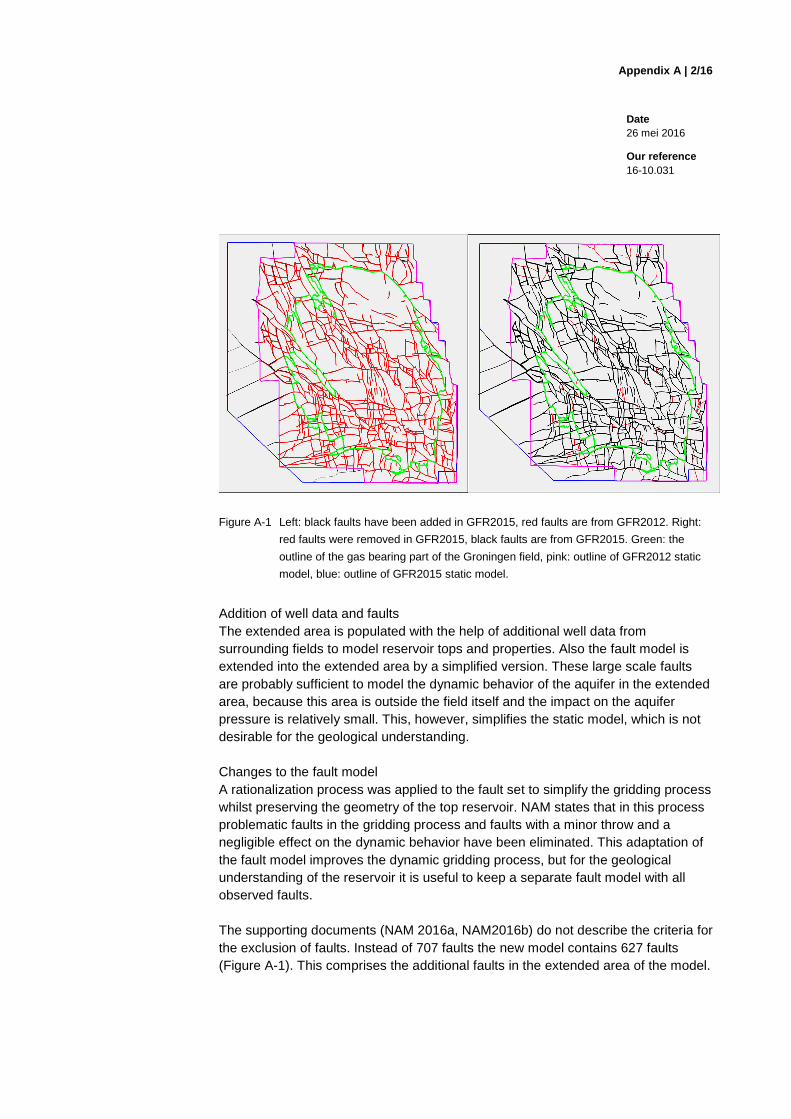
A.1.1 Structural model Extended model area The model area of the GFR2012 has been extended to the South and West (see Figure A-1); pink contour line (GFR2012) vs blue contour line (GFR2015)). The main reasons for this are the enablement of modeling subsidence in this region as well, to avoid the use of analytical aquifers and to get a constraint on the pressure depletion in the aquifer.
Appendix A | 2/16
Date 26 mei 2016 Our reference 16-10.031
Figure A-1 Left: black faults have been added in GFR2015, red faults are from GFR2012. Right:
red faults were removed in GFR2015, black faults are from GFR2015. Green: the
outline of the gas bearing part of the Groningen field, pink: outline of GFR2012 static
model, blue: outline of GFR2015 static model.
Addition of well data and faults The extended area is populated with the help of additional well data from surrounding fields to model reservoir tops and properties. Also the fault model is extended into the extended area by a simplified version. These large scale faults are probably sufficient to model the dynamic behavior of the aquifer in the extended area, because this area is outside the field itself and the impact on the aquifer pressure is relatively small. This, however, simplifies the static model, which is not desirable for the geological understanding. Changes to the fault model A rationalization process was applied to the fault set to simplify the gridding process whilst preserving the geometry of the top reservoir. NAM states that in this process problematic faults in the gridding process and faults with a minor throw and a negligible effect on the dynamic behavior have been eliminated. This adaptation of the fault model improves the dynamic gridding process, but for the geological understanding of the reservoir it is useful to keep a separate fault model with all observed faults. The supporting documents (NAM 2016a, NAM2016b) do not describe the criteria for the exclusion of faults. Instead of 707 faults the new model contains 627 faults (Figure A-1). This comprises the additional faults in the extended area of the model.
Appendix A | 3/16
Date 26 mei 2016 Our reference 16-10.031
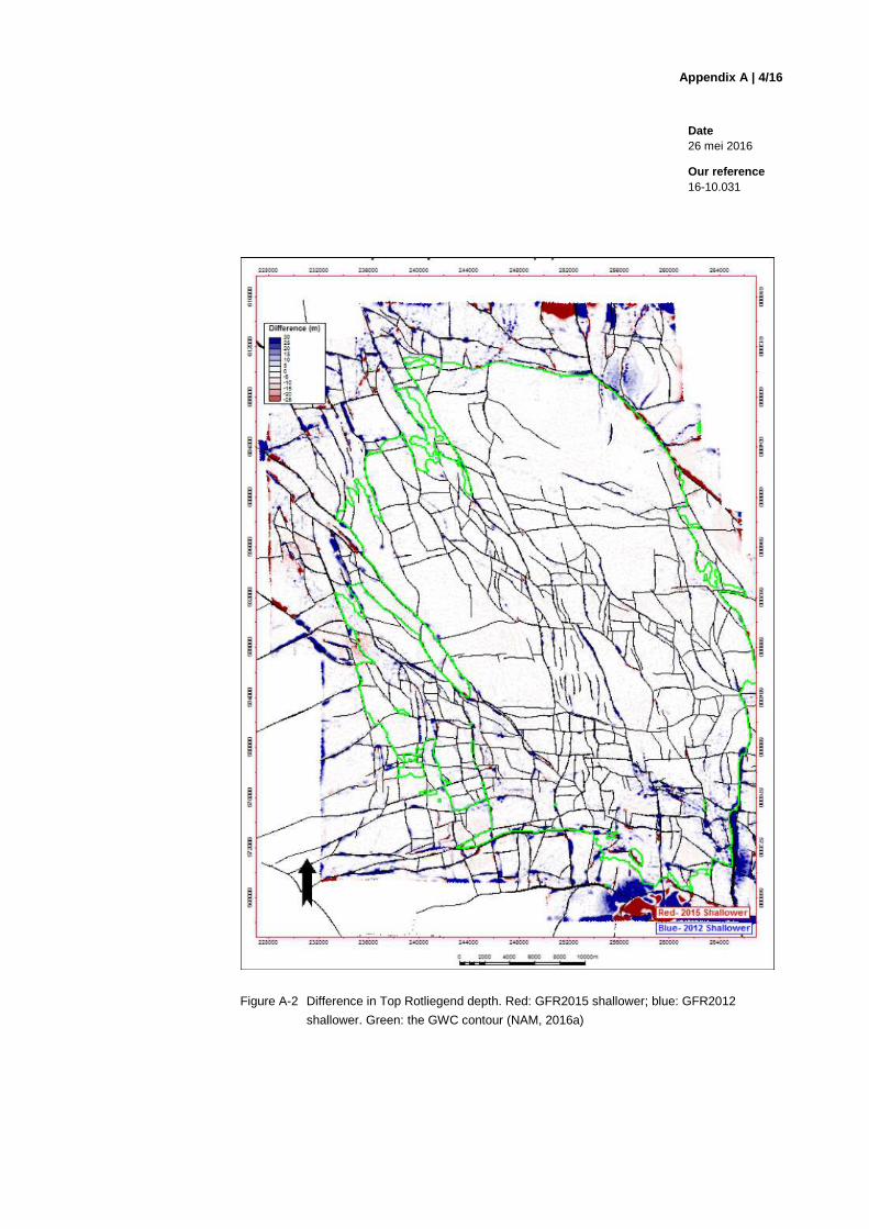
Revised Top Rotliegend map Due to the extension of the model area, the rationalized fault set and the expanded set of well data a revision of the Top Rotliegend map has been made. A significant difference lies in the number of wells used. In the GFR2012, 104 wells were excluded from the model, in the GFR2015 only 5. In these 5 wells the Top Rotliegend has been faulted out. The wells that are additionally incorporated in the GFR2015 model (located mainly in the South of the field) have a relatively high residual, but the difference between GFR 2012 and GFR 2015 still is relatively small inside the boundary of the field: the gas bearing gross rock volume of the GFR2015 is only 0.7% higher than that of the GFR2012. In the northern and southern parts of the modeled area the differences between the GFR2012 and GFR2015 Top Rotliegend map are more significant (Figure A-2).
Changes in model architecture The model architecture has been changed with respect to the GFR2012 model. In the GFR2012 version, the LSS.1.res zone was modeled with an onlap configuration, while the other zones were modeled proportionally (wedge configuration). In the GFR2015 static model a wedge configuration has been applied to all zones. This is contradictory with the information provided by NAM in the technical addendum of the 2016 production plan (NAM, 2016c), where they state on page 54 that “the Silverpit- and Slochteren Formations form a wedge of continental sediments that is onlapping southwards onto the Carboniferous relief”. TNO prefers an onlap configuration for all Ameland and Lower Slochteren zones (TNO, 2013). The AI 2003 cube was not available to TNO to verify, whether that information supports the onlap model or not. The number of layers within the zones has been changed slightly. Two versions of the model have been created, a fine model and a course model. The course model is used to create the pseudo porosity property (pseudo porosity is based on Acoustic Impedance and used for the formation of trend maps), while the fine model was used for the final porosity model. In the fine model the number of zones of the Lower Slochteren has been reduced from 59 to 30, while in the course model the number of layers in the Upper Slochteren has been increased from 8 to 16 to create more detail and a better representation of the heterogeneity.
Appendix A | 4/16
Date 26 mei 2016 Our reference 16-10.031
Figure A-2 Difference in Top Rotliegend depth. Red: GFR2015 shallower; blue: GFR2012
shallower. Green: the GWC contour (NAM, 2016a)

Appendix A | 5/16
Date 26 mei 2016 Our reference 16-10.031
A.1.2 Petrophysics Implementation of new data NAM has added newly available well data from the last years to the model. Exclusion of anomalous data The documentation provided with respect to the petrophysical updates was limited. It is stated in NAM (2016b) that anomalous data in the VCL (Clay Volume) and PORNET (Porosity) input logs was present and therefore these logs have been updated. Although no information is given about what values are considered anomalous, the effect on the property model is limited. This is shown by comparing histograms of the VCL and PORNET input logs of the GFR2012 and GFR2015 (Figure A-3).

Appendix A | 6/16
Date 26 mei 2016 Our reference 16-10.031
Figure A-3 Comparing histograms of the GFR2012 and GFR2015. a) VCL histogram (yellow:
GFR2012, green: GFR2015). b) PORNET histogram (pink: GFR2012, blue:
GFR2015). (NAM, 2016a)
a)
b)
Appendix A | 7/16
Date 26 mei 2016 Our reference 16-10.031
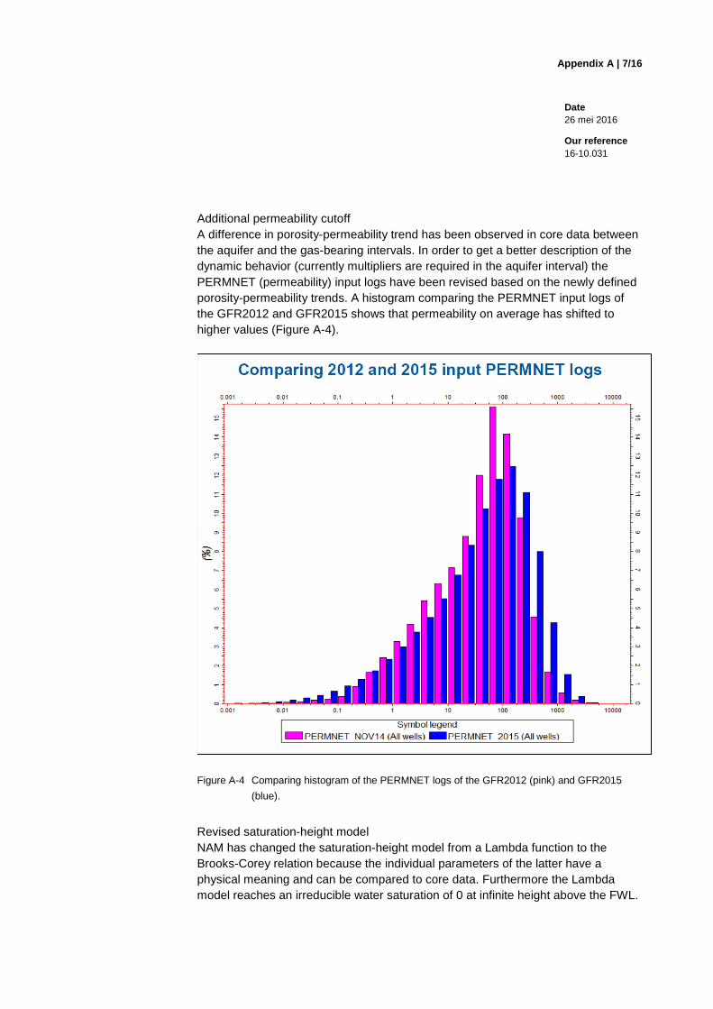
Additional permeability cutoff A difference in porosity-permeability trend has been observed in core data between the aquifer and the gas-bearing intervals. In order to get a better description of the dynamic behavior (currently multipliers are required in the aquifer interval) the PERMNET (permeability) input logs have been revised based on the newly defined porosity-permeability trends. A histogram comparing the PERMNET input logs of the GFR2012 and GFR2015 shows that permeability on average has shifted to higher values (Figure A-4).
Figure A-4 Comparing histogram of the PERMNET logs of the GFR2012 (pink) and GFR2015
(blue).
Revised saturation-height model NAM has changed the saturation-height model from a Lambda function to the Brooks-Corey relation because the individual parameters of the latter have a physical meaning and can be compared to core data. Furthermore the Lambda model reaches an irreducible water saturation of 0 at infinite height above the FWL.

Appendix A | 8/16
Date 26 mei 2016 Our reference 16-10.031
Therefore a correction is needed, which is not preferable. No details are provided by NAM on the effect of this change in the model. However, it should not make a very large difference because the functional shape of the models is similar and the individual parameters of the Lambda model were already chosen to fit the log saturation best.
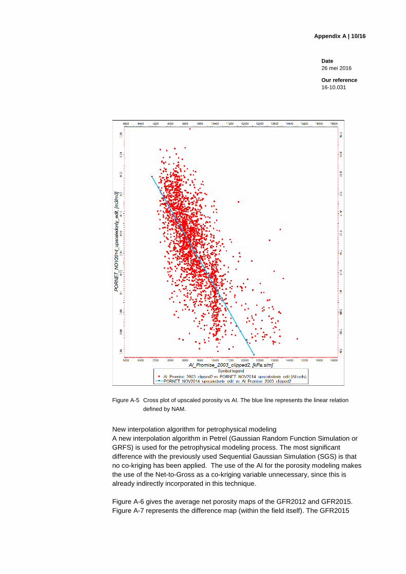
A.1.3 Property modelling Revised trend maps The methodology of creating the trend maps used for modeling clay volume and porosity has been slightly changed. Firstly, instead of manually selecting a representative value for a production cluster, now the highest and lowest values are discarded and the remaining data points are averaged. This adds some statistical meaning to the values for production clusters. Secondly, functional interpolation instead of isochore interpolation is used to create the trend maps. Functional interpolation creates a 3D function that is used for interpolation. Cell values are interpolated weighed with distance to the input data. This is a significant improvement since isochore interpolation can over- or underestimate properties in between wells, while functional interpolation cannot. Furthermore, functional interpolation creates a smoother map that represents a more regional trend map. Changes in Data Analysis NAM has revised the data analysis step in Petrel in three ways. Firstly, the way of determining major and minor variogram orientations has been changed. Secondly, the trend maps are no longer used as co-kriging trend in the petrophysical modeling. They are now input for the different data analysis steps of which the results are used for the petrophysical modeling. Thirdly, where appropriate, nested variograms are used to represent multiple correlation lengths in a single data distribution. These changes are an optimization of the use of trend maps. Porosity model based on Acoustic Impedance The GFR2015 porosity model is based on an acoustic impedance (AI) cube from 2003. It uses porosity from wells as calibration. NAM has announced that an updated version of the AI is underway. This update will be part of the GFR2016 V3.0 update in the second half of 2016. The AI method has been suggested by TNO (TNO, 2013). A linear relation has been defined between up scaled porosity logs and the seismically resampled AI cube. This relation has been used to create pseudo-porosity trend maps. These trend maps were the input for the data analysis and petrophysical modeling. The definition of this relation has a large impact on the resulting porosity model, because it governs the calculation of porosity in between wells. A cross plot of the up scaled well log porosity versus the resampled AI (Figure A-5) shows a fairly scattered data cloud. Also some kind of cutoff seems to be present at around 10400 kPa·s/m, which is not explained. NAM defined a single linear relation through this

Appendix A | 9/16
Date 26 mei 2016 Our reference 16-10.031
data cloud, that visually does not give a proper fit to the data (Figure A-5). The slope of the relation is smaller than the visual trend in the data cloud. This might be the effect of the low porosity – high AI data points in the plot. Furthermore, the shape of the data cloud suggests a curved rather than a linear relation. The scattered data cloud introduces a certain level of uncertainty to the porosity model. The defined relation is probably underestimating the higher porosity and overestimating the lower porosity regions. However, at the well locations the porosity is equal to the petrophysical averages. The uncertainty of this relation should have been captured by an uncertainty bandwidth in the porosity model, which is currently not available. The documentation provided by NAM (NAM, 2016b) states that pseudo-porosity trend maps are used for the reservoir zones. The previous log-derived trend maps are used for the heterolithic and Ten Boer zones. This is because the inversion result of these layers shows a large scatter. The scatter derives from the sub-seismic thickness of the heterolithic zones and the less suitable petrophysical model for clay rich zones. However, the data analysis in the delivered Petrel project shows, that for the heterolithic zones the pseudo-porosity maps of the underlying reservoir zone are used.
Appendix A | 10/16
Date 26 mei 2016 Our reference 16-10.031
Figure A-5 Cross plot of upscaled porosity vs AI. The blue line represents the linear relation
defined by NAM.
New interpolation algorithm for petrophysical modeling A new interpolation algorithm in Petrel (Gaussian Random Function Simulation or GRFS) is used for the petrophysical modeling process. The most significant difference with the previously used Sequential Gaussian Simulation (SGS) is that no co-kriging has been applied. The use of the AI for the porosity modeling makes the use of the Net-to-Gross as a co-kriging variable unnecessary, since this is already indirectly incorporated in this technique. Figure A-6 gives the average net porosity maps of the GFR2012 and GFR2015. Figure A-7 represents the difference map (within the field itself). The GFR2015

Appendix A | 11/16
Date 26 mei 2016 Our reference 16-10.031
porosity map shows a more locally defined expression of porosity than the GFR2012 map. Furthermore, the porosity in certain areas fits better with the measured porosity, e.g. around Bedum in the Western flank of the field. The difference map (Figure A-7) shows that the overall porosity of the GFR2015 is slightly lower than the GFR2012. This is mainly due to the new AI input and the relation between porosity and AI.

Appendix A | 12/16
Date 26 mei 2016 Our reference 16-10.031
Figure A-6 a) GFR2012 average net porosity; b) GFR2015 average net porosity.
a)
b)

Appendix A | 13/16
Date 26 mei 2016 Our reference 16-10.031
Figure A-7 Difference map between GFR2015 and GFR2012 porosity model. Red: GFR2015
porosity is lower; blue: GFR2012 porosity is lower.
A.2 Model evaluation in view of recommendations by TNO in
2013
The report by TNO (2013) on the evaluation of the GFR2012 static model contains a number of recommendations for future improvements of the model. This section discusses to what extent these recommendations are addressed in the updated GFR2015 model.
1. Use all faults visible in the seismic for the geomechanical study, not only the 707 modeled faults from the GFR2012 model. NAM has removed and merged faults within the current fault set. This is done to simplify the gridding process. This simplification probably improves the simulation of the dynamic behavior in the field and is therefore useful for the evaluation of the production strategy. On the other hand, for detailed geological understanding of the reservoir architecture and in particular geomechanical and seismological studies the current fault model is too simplistic.
Appendix A | 14/16
Date 26 mei 2016 Our reference 16-10.031
2. Apply onlap architecture to all Lower Slochteren and Ameland zones or prove that the use of a wedge configuration above the LSS.1.res zone has no effect on the property modeling. NAM modeled all zones proportionally (wedge configuration) in the GFR2015 model. The currently available documentation (NAM, 2016a; NAM, 2016b) does not describe the reasoning of NAM to choose this model.
3. If possible use other parameters to control the porosity modeling, e.g. acoustic impedance or facies models. NAM used an acoustic impedance cube to calculate the porosity model of the GFR2015. This is a significant improvement compared to the modeling method of the GFR2012. In the GFR2015 porosity in between wells is calculated using the AI, which is a physical rock property that gives a better control on porosity. Information about sedimentological facies is still not taken into account, but since the AI is used as input for the porosity model, this is of less importance than it was for the GFR2012 model.
4. Take into account the uncertainty bandwidth in the porosity modeling process and use this in further subsidence calculations. The GFR2015 static model represents one realization of the porosity model only; no uncertainty bandwidth of porosity and subsidence has been calculated by NAM. Although it would still have been useful if a calculation of the uncertainty of the GFR2015 porosity model was presented, it is of less importance than it was for the GFR2012 model because of the difference in modeling methods. The uncertainty estimation is especially important for the areas between well locations, given the control on porosity at well locations by the petrophysical averages. In the GFR2012 model no geological or physical control was used to calculate porosity between wells (trend maps were based on well data). However, the GFR2015 model is based on the acoustic impedance, which is a physical rock property, and its relation with porosity. Therefore more control on porosity is present between the wells, resulting in a significantly reduced uncertainty. Facies modeling might further enhance the compaction modeling.
5. Further explain some of the outstanding phenomena in the current model in terms of geology and modeling and determine the possible influence on subsidence calculations. At the moment of writing no detailed report of the GFR2015 static model was available to TNO-AGE.
Appendix A | 15/16
Date 26 mei 2016 Our reference 16-10.031
6. Calculate porosity based on modeled subsidence. The discrepancy between the calculated and measured subsidence can possibly be explained when inverse porosity lies within the uncertainty bandwidth of the porosity model. This calculation has not been performed by NAM for the GFR2015. Although the uncertainty bandwidth is probably significantly reduced by the new modeling method.
A.3 Findings
In this evaluation the GFR2015 static model is compared with the GFR2012 static model to determine and assess the applied changes in terms of model improvement. The main findings are: Structural model: • The fault set has been rationalized by removing and merging a selection of
faults. This improves the simulation of the dynamic behavior, but simplifies the static model, which is not desirable for the geological understanding.
• The Top Rotliegend map has been improved, due to an extended set of well data in the original model area and the addition of faults and well data in the extended model area.
• Only a wedge configuration has been applied to all zones of the static model.
Petrophysics: • Minor changes have been applied to the Clay Volume and Porosity input logs,
which only have a small effect on the resulting porosity model. • The porosity-permeability relation has changed. Instead of a single relation for
the whole reservoir, two separate exponential relations have been defined for the gas filled reservoir and the aquifer interval. This has a significant effect on the permeability in the gas filled reservoir, which generally has shifted to higher values.
Property model: • The process of creating trend maps has been improved by using functional
interpolation instead of isochore interpolation. Furthermore, the porosity at cluster locations is defined differently.
• The Acoustic Impedance has been used as input for the GFR2015 static model. This is an improvement of the model, since it provides a physical control of the porosity in between well locations and significantly reduces the uncertainty on porosity.

Appendix A | 16/16
Date 26 mei 2016 Our reference 16-10.031
References NAM (2016a) Groningen Field – Static model update (Draft). NAM (2016b) Groningen static model update 2015 (Draft). NAM (2016c) Technical Addendum to the Winningsplan Groningen 2016.
Production, Subsidence, Induced Earthquakes and Seismic Hazard and Risk Assessment in the Groningen Field.
TNO (2013) Toetsing van de bodemdalingsprognoses en seismische hazard ten
gevolge van gaswinning van het Groningen veld. TNO Report R11953.
Appendix B | 1/8
|
B Dynamic Model Review
The update of the dynamic model of the Groningen field is reviewed. A full overview of the match in all wells and of the spatial distribution of the match is beyond the scope of this review. The review is based on the following NAM information and documents:
• MoReS model: GRO_2015_ED_v34_v9.run (received Feb 2016) • Technical Addendum to the Winningsplan Groningen 2016: Production,
Subsidence, Induced Earthquakes and Seismic Hazard and Risk Assessment in the Groningen Field Part I Summary & Production
• Groningen Field Review 2015; Subsurface Dynamic Modelling Report (Restricted). GFR2015_report_draft_20160316.pdf:
Note that the Groningen Field Review 2015 document is an incomplete, restricted draft that contains some inconsistencies: the layering is described for a model that has 34 layers, but the model GRO_2015_ED_v34_v9.run has 30 layers. Therefore this report is used as little as possible. Changes from the GFR2012 to the GFR2015 model are discussed against the background of recommendations made in TNO (2013 and 2014).
B.1 Model changes
B.1.1 Aquifer modeling The main recommendation (TNO, 2013) is to improve aquifer modelling and to extend the model to peripheral areas, especially in the north-west. This part received a complete overhaul. The main changes in the GFR2015 model are: • extension of the model area to include peripheral gas fields and a larger part of
the aquifers; • taking into account the additional measurements in these areas and newly
drilled wells; • changes to the aquifer modelling (numerical versus analytical);. • including subsidence data in the history matching workflow; • fault sealing.
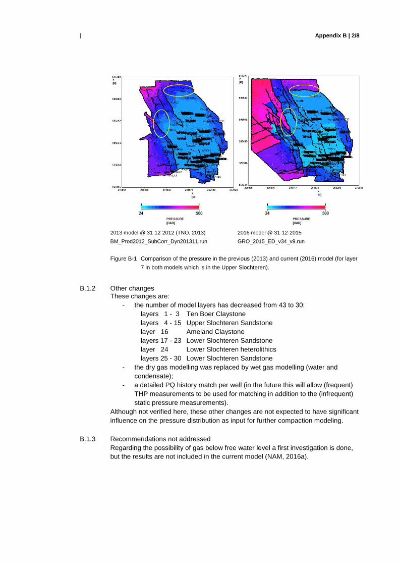
The effect of the introduction of sealing faults is most noticeable in the North and North-west areas. It results in sharper pressure contrasts, where the previous model shows gradual changes (Figure B-1). Pressure wise, two areas are especially affected: north of UHM-1A and the fault block just west of BHR-1 (indicated by ellipses).
Appendix B | 2/8
|
2013 model @ 31-12-2012 (TNO, 2013)
BM_Prod2012_SubCorr_Dyn201311.run
2016 model @ 31-12-2015
GRO_2015_ED_v34_v9.run
Figure B-1 Comparison of the pressure in the previous (2013) and current (2016) model (for layer
7 in both models which is in the Upper Slochteren).
B.1.2 Other changes
These changes are: - the number of model layers has decreased from 43 to 30:
layers 1 - 3 Ten Boer Claystone layers 4 - 15 Upper Slochteren Sandstone layer 16 Ameland Claystone layers 17 - 23 Lower Slochteren Sandstone layer 24 Lower Slochteren heterolithics layers 25 - 30 Lower Slochteren Sandstone
- the dry gas modelling was replaced by wet gas modelling (water and condensate);
- a detailed PQ history match per well (in the future this will allow (frequent) THP measurements to be used for matching in addition to the (infrequent) static pressure measurements).
Although not verified here, these other changes are not expected to have significant influence on the pressure distribution as input for further compaction modeling.
B.1.3 Recommendations not addressed
Regarding the possibility of gas below free water level a first investigation is done, but the results are not included in the current model (NAM, 2016a).

Appendix B | 3/8
|
B.2 History match
B.2.1 Model multipliers Multipliers used in the model are:
- 24 global and local multipliers on Gross Block Volume (net reservoir grid block volumes) and permeability;
- 38 sealing factors on groups of faults; - other tuning parameters like aquifer properties, well inflow properties (skin)
etc.; - field-wide permeability multipliers in z-direction, applied on the Ten Boer
Claystone, Ameland Claystone ( 2.5·10-3) and Lower Slochteren heterolithics (1·10-2);
- for the Ten Boer Claystone also permeability multipliers in x- and y-direction.
B.2.2 Quality of the pressure history match
The changes described above result in a much improved match to observed pressures (e.g. USQ, Figure B-1). For the wells shown in (NAM, 2016), the fit to the GWC rise has improved. However, the change to the GWC contact rise in the north-western part of the model could not be evaluated. This is because the results for these wells are not shown in (NAM, 2016) and the results are not incorporated in the MoReS model available to TNO. In this area the rise in GWC is clearly overestimated in the 2013 model (wells ZRP-1 and SDM-1; TNO, 2013). Increasing the faults sealing should have improved that. In the previous model the uncertainty of the model in the south-west corner was very high (TNO, 2013). This has improved (e.g. pressure match in wells HRS-2A, TBR-4 and EKL-13).
B.2.3 Subsidence match
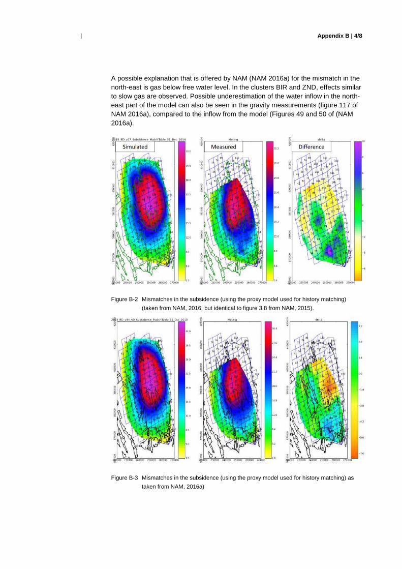
Two versions of the match to subsidence are available: Figure B-2 shows the figure from NAM (2016)1. Figure B-3 shows the version from NAM (2016a), which is the most recent model (GRO_2015_ED_v34_v9 according to the caption on top of the model). For both cases, the subsidence is generally overestimated by the model in the north part of the field and underestimated in the southern part. In the most recent version the subsidence caused by salt mining south of the Groningen field is excluded from the measured data, which was not done for the previous version. This explains the large mismatch seen in Figure B-2 between measured and simulated subsidence in the south of the Groningen field (purple blob), which is not observed for the most recent model. In the south of the model (Figure B-3), there is an area where the subsidence is underestimated.
1 which appears to be Figure 3.8 from the Hazard and Risk Assessment Interim Update from November 2015 (NAM, 2015) (model version GRO_2015_ED_v27_hra).
Appendix B | 4/8
|
A possible explanation that is offered by NAM (NAM 2016a) for the mismatch in the north-east is gas below free water level. In the clusters BIR and ZND, effects similar to slow gas are observed. Possible underestimation of the water inflow in the north-east part of the model can also be seen in the gravity measurements (figure 117 of NAM 2016a), compared to the inflow from the model (Figures 49 and 50 of (NAM 2016a).
Figure B-2 Mismatches in the subsidence (using the proxy model used for history matching)
(taken from NAM, 2016; but identical to figure 3.8 from NAM, 2015).
Figure B-3 Mismatches in the subsidence (using the proxy model used for history matching) as
taken from NAM, 2016a)

Appendix B | 5/8
|
B.2.4 Aquifer modelling and water inflow In Table B-1 the analytical aquifers in the current model (GRO_2015_ED_v34_v9) are listed. A large change is the aquifer inflow in the north-west part of the model. In the previous model (see TNO, 2014), considerable water inflow from strong aquifers is required to simulate the lack of subsidence (presumably caused by a lack in pressure drop) in this region. In the current model, the attached aquifers are still quite large (see length of Moewensteert and Rodewolt in Table B-1). However, due to (assumed) sealing faults in this area the inflow has become considerably smaller (compare Figure B-4 and Figure B-5, please note the difference in scale). The largest inflow is still in approximately the same area, but much smaller (approx. factor 100). Figure B-6 shows the cumulative aquifer inflow over time. It shows that the modeled total inflow to the Groningen field has reduced considerably. Increasing the fault seals appears to be an adequate solution to improve the history match and reduce the aquifer inflow. It is not clear at this point, whether there are additional reasons, as to why these particular faults are chosen to be sealing other than the dynamic data. Notice for example faults ‘B44b’ and ‘mFS16 Fault S’ in Figure 2.1-8 in (NAM, 2016), which have only a relatively small offset.
Table B-1 Overview of analytical aquifers in the current model (GRO_2015_ED_v34_v9.run)
Name Location Length (km)
AnnerveenVeendam South 1.5 Lauwersee1 South-west 6 Lauwersee2 South-west 1 Lauwersee3 South-west 1 Lauwersee4 South-west 3 Moewensteert North 35 Rodewolt North-west 10 Rysum East 5 Usquert North 1

Appendix B | 6/8
|
Figure B-4 Aquifer inflow (indicated by bars on the edge of the model) in the north of the model
(GRO_2015_ED_v34_v9_noforecast_SFA.run @ 31-12-2015).
Figure B-5 Aquifer inflow (indicated by bars on the edge of the model) in the north of the model
(BM_Prod2012_SubCorr_Dyn201311.run @ 31-12-2012) discussed in (Thienen-
Visser et al., 2014).

Appendix B | 7/8
|
Figure B-6 Comparison of the cumulative aquifer inflow for the 2013 model used for (TNO, 2013)
and the updated model GRO_2015_ED_v34_v9.run.
B.3 Main findings
The current dynamic reservoir model is more suited for the purpose of estimating and forecasting the subsidence than the previous model, because of: • an increase in model area over the peripheral aquifers and gas fields, • inclusion of subsidence as a measurement in the history matching workflow, • reduction of inflow from analytical aquifers, better match with observed inflow
and subsidence; • an improved history match in the peripheral areas of the model (as far as could
be evaluated).
It is noted that the dynamic model description document (GFR 2015) as provided by the NAM was an incomplete draft. Therefore, our review is incomplete. The review was at a regional level: detailed review of the model history match at individual well (cluster) level was beyond the scope.
Appendix B | 8/8
|
References NAM (2015) Hazard and Risk Assessment for Induced Seismicity in Groningen,
Interim Update November 2015. EP201511200172 NAM (2016) Technical Addendum to the Winningsplan Groningen 2016:
Production, Subsidence, Induced Earthquakes and Seismic Hazard and Risk Assessment in the Groningen Field Part I Summary & Production
NAM (2016a) Groningen Field Review 2015; Subsurface Dynamic Modelling
Report. Restricted. Incomplete draft. TNO (2013) Toetsing van de bodemdalingsprognoses en seismische hazard ten
gevolge van gaswinning van het Groningen veld. TNO2013 R11653. TNO (2014) Recent developments of the Groningen field in 2014 and,
specifically, the southwest periphery of the field. TNO2014 R11703.
Appendix C | 1/19
|
C Compaction and subsidence
Compaction and subsidence calculations of the Groningen field, as presented by NAM in their production plan 2016 (further called WP2016), are evaluated and checked. Results are presented in section C.1, where TNO (2013) is used as a reference. In addition, the subsidence forecasts presented in the WP2016 are evaluated. These results are given in section C.2.
C.1 Compaction modelling
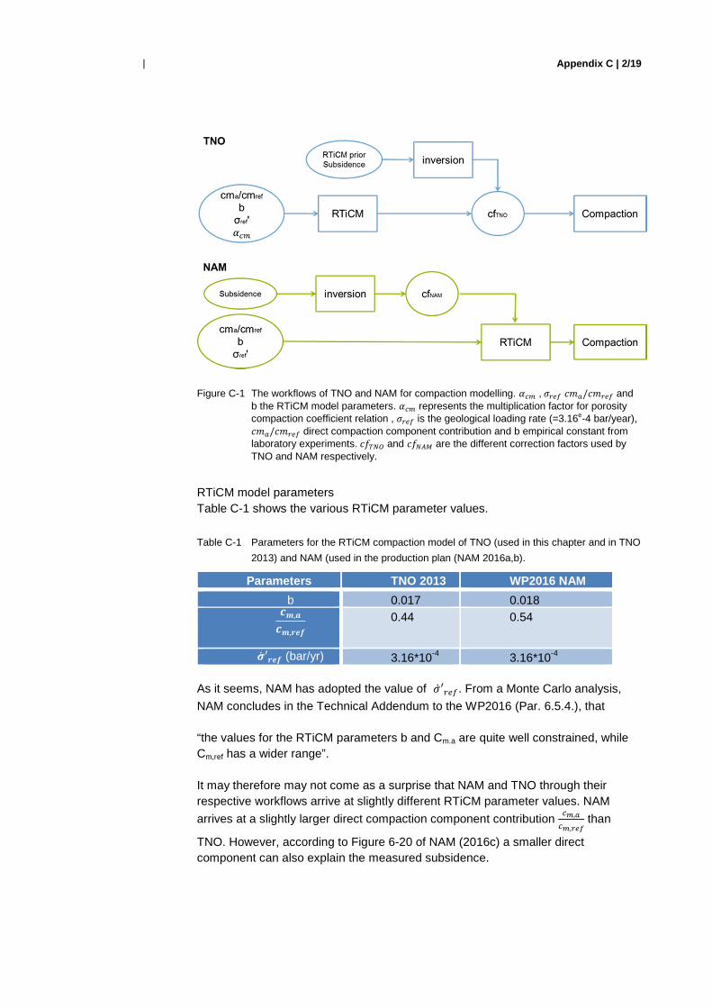
C.1.1 Compaction model In WP2016 the NAM has chosen the rate type compaction model in isotach formulation (RTiCM, Pruiksma et al., 2015) as base model in line with TNO (2013). Inversion scheme Results from laboratory tests on the relationship between compaction coefficient and porosity show a large scatter: for a given porosity, the measured compaction coefficient typically has a variability of a factor 5. This complicates the direct application of a relationship directly derived from these lab tests. For this reason a subsidence inversion scheme was proposed to enhance the consistency with observed subsidence (Fokker and Van Thienen-Visser 2016). In WP2016 NAM uses a subsidence inversion scheme. The workflows are different in some aspects:
- NAM uses as a prior the laboratory derived Cm-porosity relationship from WP2013;
- TNO uses as prior a forward calculated compaction field, computed from the subsurface model and the RTiCM compaction (presented in TNO 2013) model. This compaction field was fitted to the subsidence data by applying a multiplier ��� = 0,57 to the laboratory derived Cm-porosity relationship.
In Figure C-1, both TNO and NAM’s compaction processing chain is explained by two flowcharts.
Appendix C | 2/19
|
Figure C-1 The workflows of TNO and NAM for compaction modelling. ��� ,�� � �/� � and b the RTiCM model parameters. ��� represents the multiplication factor for porosity compaction coefficient relation , �� is the geological loading rate (=3.16e-4 bar/year), � �/� � direct compaction component contribution and b empirical constant from laboratory experiments.����� and ����� are the different correction factors used by TNO and NAM respectively.
RTiCM model parameters Table C-1 shows the various RTiCM parameter values.
Table C-1 Parameters for the RTiCM compaction model of TNO (used in this chapter and in TNO
2013) and NAM (used in the production plan (NAM 2016a,b).
Parameters TNO 2013 WP2016 NAM
b 0.017 0.018 ��,�
��,���
0.44 0.54
�� ′��� (bar/yr) 3.16*10-4 3.16*10-4 As it seems, NAM has adopted the value of �� ′�. From a Monte Carlo analysis,
NAM concludes in the Technical Addendum to the WP2016 (Par. 6.5.4.), that “the values for the RTiCM parameters b and Cm.a are quite well constrained, while Cm,ref has a wider range”. It may therefore may not come as a surprise that NAM and TNO through their respective workflows arrive at slightly different RTiCM parameter values. NAM
arrives at a slightly larger direct compaction component contribution ��,�
��, !" than
TNO. However, according to Figure 6-20 of NAM (2016c) a smaller direct component can also explain the measured subsidence.
Appendix C | 3/19
|
It is important to note here, that NAM and TNO have based their analysis on one and the same static and dynamic model realization: the influence of any uncertainty in these models is not explicitly accounted for in the compaction and subsidence workflows.
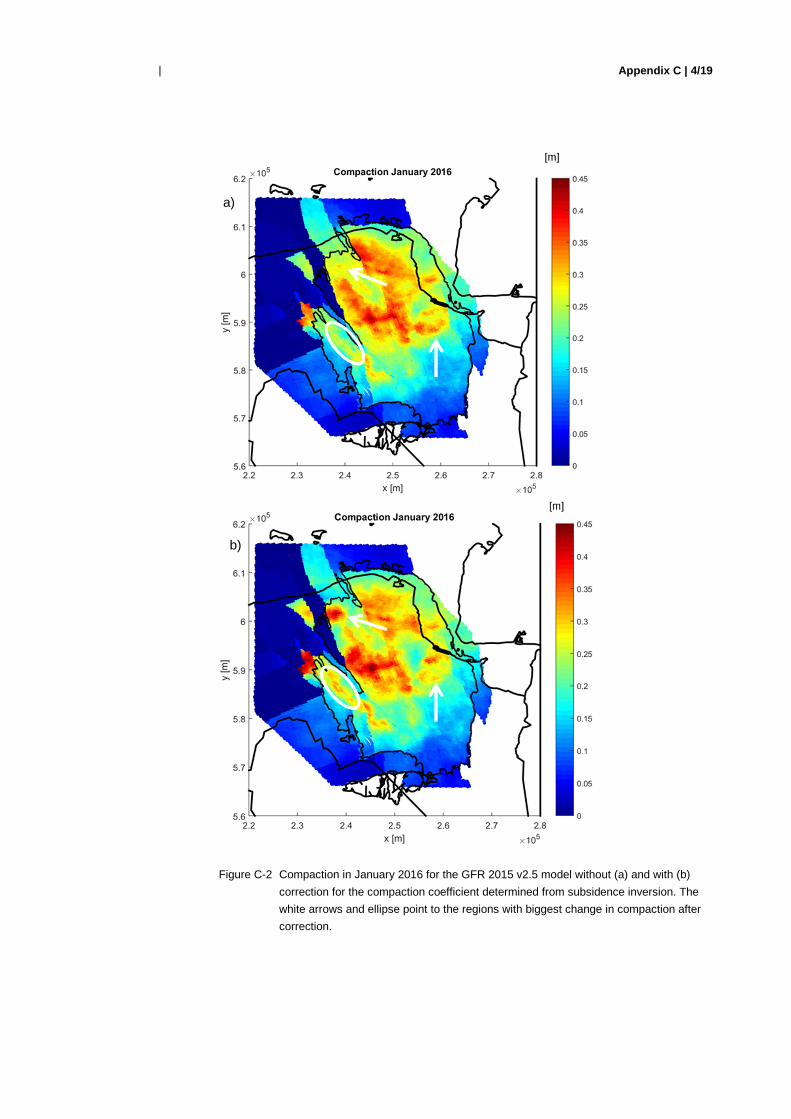
C.1.2 Effect on the compaction field of inversion derived correction factors in the TNO workflow The results of the subsidence inversion are used as a correction on the compaction field. Figure C-2 shows the compaction in January 2016 for the GFR 2015 v2.5 model without and with these correction factors applied. Compaction is clearly different at the locations identified by the ellipse and the arrows. Figure C-3 shows the difference between measured and calculated subsidence in the year 2011 for GFR 2015 v 2.5 model without (a) and with (b) correction for compaction coefficient determined from subsidence inversion. Clearly, the introduction of correction factors has decreased the mismatch between calculated and measured subsidence. Not surprisingly, since the correction factors are the result of a subsidence inversion, which used the measured subsidence as an input. The largest difference between measured and calculated subsidence is in the northwestern part of the field. The fit in the western part of the field, close to Groningen, improved substantially.
Appendix C | 4/19
|
Figure C-2 Compaction in January 2016 for the GFR 2015 v2.5 model without (a) and with (b)
correction for the compaction coefficient determined from subsidence inversion. The
white arrows and ellipse point to the regions with biggest change in compaction after
correction.
a)
b)

Appendix C | 5/19
|
Figure C-3 . Difference between measured and calculated subsidence (in 2011) for GFR 2015 v
2.5 without (a) and with (b) correction for compaction coefficient determined from
subsidence inversion. Red values indicate more subsidence calculated than
measured, blue less subsidence calculated than measured.
a)
b)
Appendix C | 6/19
|
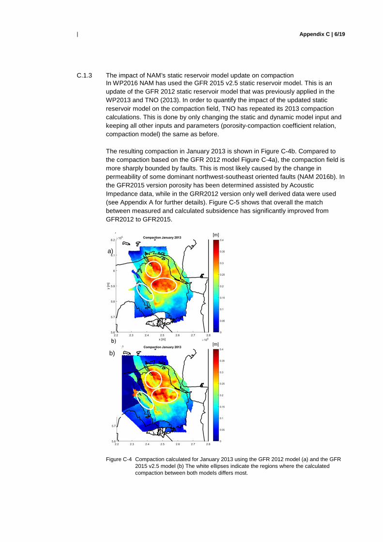
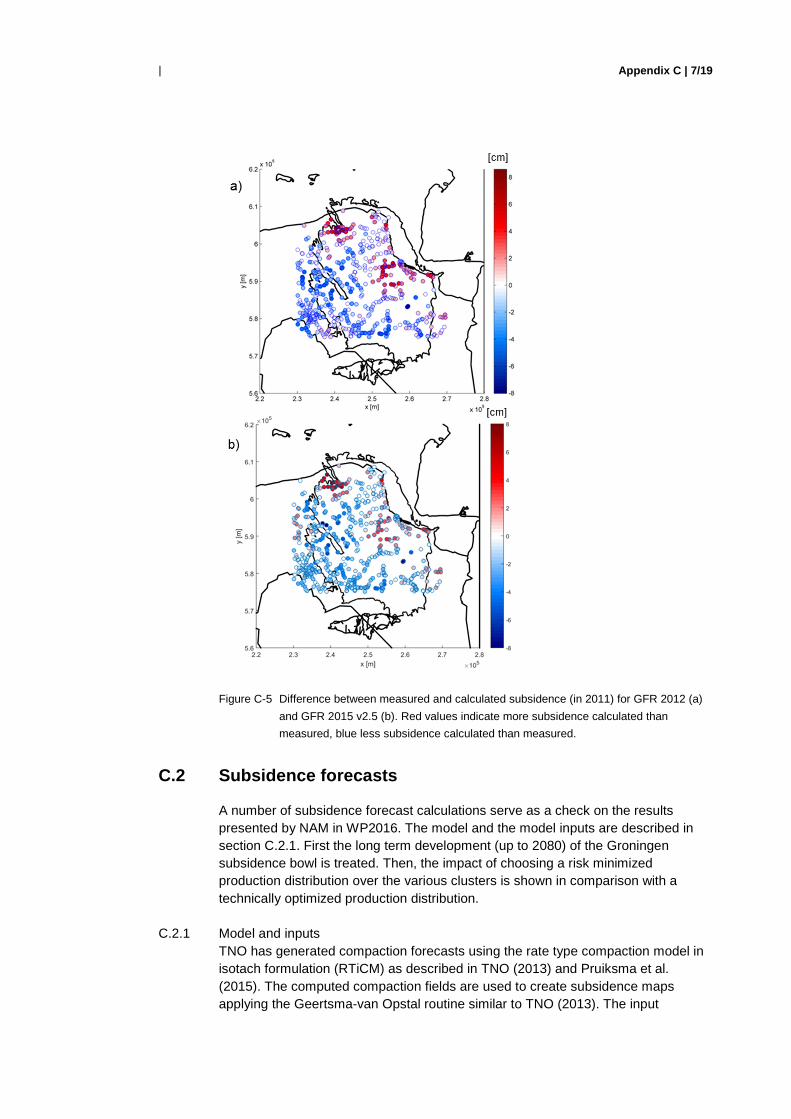
C.1.3 The impact of NAM’s static reservoir model update on compaction In WP2016 NAM has used the GFR 2015 v2.5 static reservoir model. This is an update of the GFR 2012 static reservoir model that was previously applied in the WP2013 and TNO (2013). In order to quantify the impact of the updated static reservoir model on the compaction field, TNO has repeated its 2013 compaction calculations. This is done by only changing the static and dynamic model input and keeping all other inputs and parameters (porosity-compaction coefficient relation, compaction model) the same as before. The resulting compaction in January 2013 is shown in Figure C-4b. Compared to the compaction based on the GFR 2012 model Figure C-4a), the compaction field is more sharply bounded by faults. This is most likely caused by the change in permeability of some dominant northwest-southeast oriented faults (NAM 2016b). In the GFR2015 version porosity has been determined assisted by Acoustic Impedance data, while in the GRR2012 version only well derived data were used (see Appendix A for further details). Figure C-5 shows that overall the match between measured and calculated subsidence has significantly improved from GFR2012 to GFR2015.
Figure C-4 Compaction calculated for January 2013 using the GFR 2012 model (a) and the GFR 2015 v2.5 model (b) The white ellipses indicate the regions where the calculated compaction between both models differs most.
a)
b)
Appendix C | 7/19
|
Figure C-5 Difference between measured and calculated subsidence (in 2011) for GFR 2012 (a)
and GFR 2015 v2.5 (b). Red values indicate more subsidence calculated than
measured, blue less subsidence calculated than measured.
C.2 Subsidence forecasts
A number of subsidence forecast calculations serve as a check on the results presented by NAM in WP2016. The model and the model inputs are described in section C.2.1. First the long term development (up to 2080) of the Groningen subsidence bowl is treated. Then, the impact of choosing a risk minimized production distribution over the various clusters is shown in comparison with a technically optimized production distribution.
C.2.1 Model and inputs TNO has generated compaction forecasts using the rate type compaction model in isotach formulation (RTiCM) as described in TNO (2013) and Pruiksma et al. (2015). The computed compaction fields are used to create subsidence maps applying the Geertsma-van Opstal routine similar to TNO (2013). The input
Appendix C | 8/19
|
pressure distribution forecasts in space and time are taken from the dynamic model, provided by NAM (see Appendix B for further details).
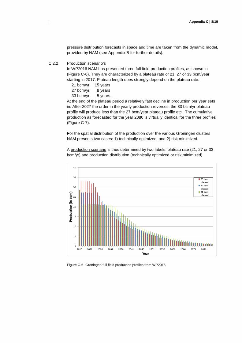
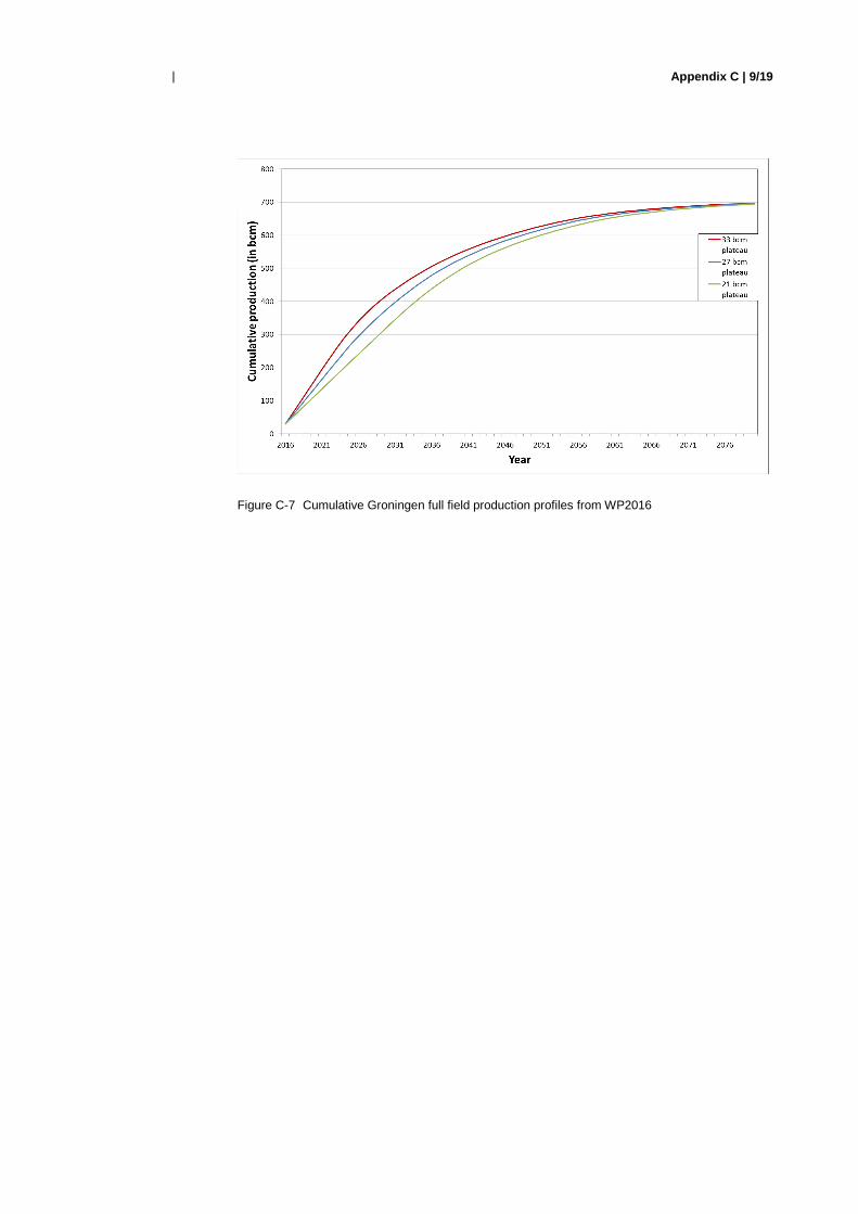
C.2.2 Production scenario’s In WP2016 NAM has presented three full field production profiles, as shown in (Figure C-6). They are characterized by a plateau rate of 21, 27 or 33 bcm/year starting in 2017. Plateau length does strongly depend on the plateau rate: 21 bcm/yr: 15 years 27 bcm/yr: 8 years 33 bcm/yr: 5 years. At the end of the plateau period a relatively fast decline in production per year sets in. After 2027 the order in the yearly production reverses: the 33 bcm/yr plateau profile will produce less than the 27 bcm/year plateau profile etc. The cumulative production as forecasted for the year 2080 is virtually identical for the three profiles (Figure C-7).
For the spatial distribution of the production over the various Groningen clusters NAM presents two cases: 1) technically optimized, and 2) risk minimized. A production scenario is thus determined by two labels: plateau rate (21, 27 or 33 bcm/yr) and production distribution (technically optimized or risk minimized).
Figure C-6 Groningen full field production profiles from WP2016
Appendix C | 9/19
|
Figure C-7 Cumulative Groningen full field production profiles from WP2016
Appendix C | 10/19
|
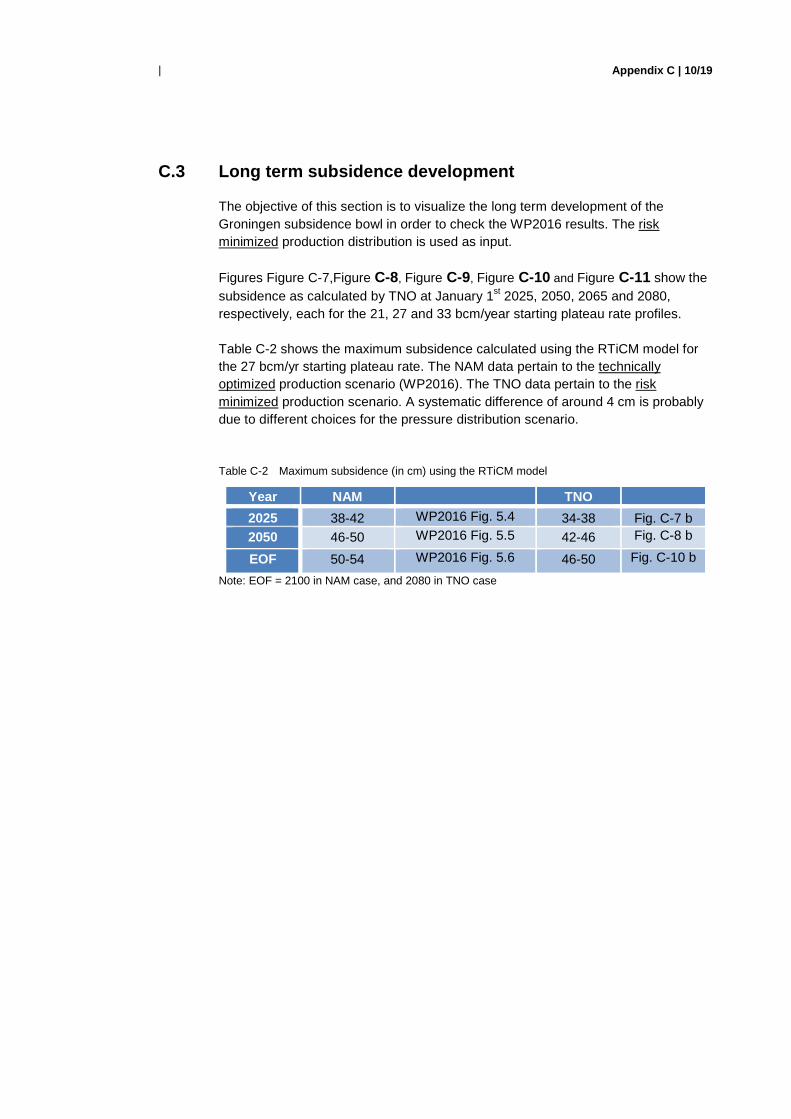
C.3 Long term subsidence development
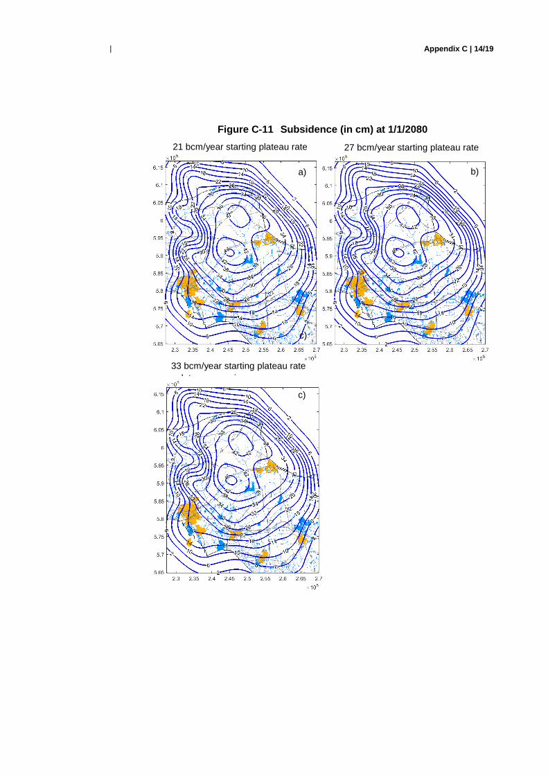
The objective of this section is to visualize the long term development of the Groningen subsidence bowl in order to check the WP2016 results. The risk minimized production distribution is used as input. Figures Figure C-7,Figure C-8, Figure C-9, Figure C-10 and Figure C-11 show the subsidence as calculated by TNO at January 1st 2025, 2050, 2065 and 2080, respectively, each for the 21, 27 and 33 bcm/year starting plateau rate profiles. Table C-2 shows the maximum subsidence calculated using the RTiCM model for the 27 bcm/yr starting plateau rate. The NAM data pertain to the technically optimized production scenario (WP2016). The TNO data pertain to the risk minimized production scenario. A systematic difference of around 4 cm is probably due to different choices for the pressure distribution scenario.
Table C-2 Maximum subsidence (in cm) using the RTiCM model
Year NAM TNO
2025 38-42 WP2016 Fig. 5.4 34-38 Fig. C-7 b 2050 46-50 WP2016 Fig. 5.5 42-46 Fig. C-8 b
EOF 50-54 WP2016 Fig. 5.6 46-50 Fig. C-10 b
Note: EOF = 2100 in NAM case, and 2080 in TNO case

Appendix C | 11/19
|
Figure C-8 Subsidence (in cm) at 1/1/2025
a) b)
c)
21 bcm/year starting plateau rate 27 bcm/year starting plateau rate
33 bcm/year starting plateau rate
Appendix C | 12/19
|
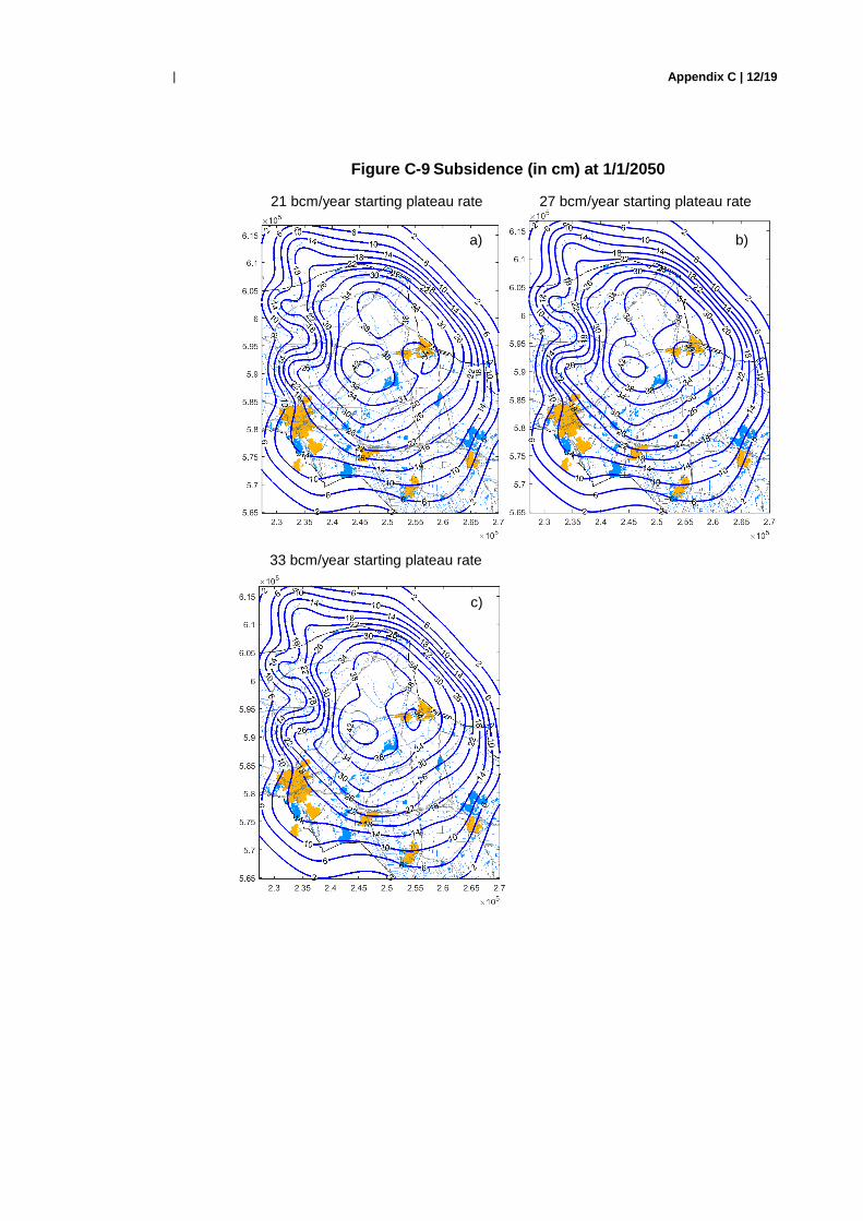
Figure C-9 Subsidence (in cm) at 1/1/2050
b)
c)
a)
21 bcm/year starting plateau rate 27 bcm/year starting plateau rate
33 bcm/year starting plateau rate
Appendix C | 13/19
|
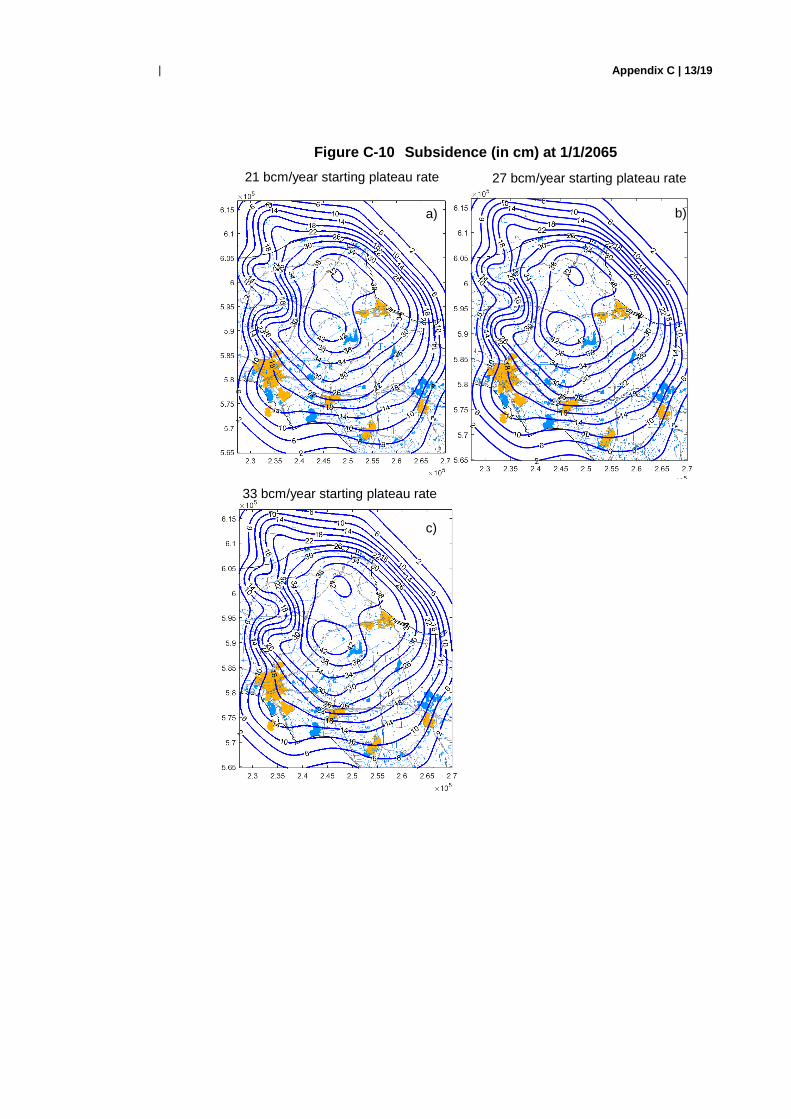
Figure C-10 Subsidence (in cm) at 1/1/2065
a) b)
c)
21 bcm/year starting plateau rate 27 bcm/year starting plateau rate
33 bcm/year starting plateau rate r
Appendix C | 14/19
|
Figure C-11 Subsidence (in cm) at 1/1/2080
c)
a) b)
c)
21 bcm/year starting plateau rate 27 bcm/year starting plateau rate
33 bcm/year starting plateau rate pplateauscenario
Appendix C | 15/19
|
C.4 Impact of the risk minimized production distribution on subsidence
The objective of this section is to visualize the impact on the pattern of incremental subsidence of the chosen production distribution. To this end TNO has calculated incremental subsidence for the next 5 and 10 years, in each case for the 21, 27 and 33 bcm/year plateau rate profiles.
C.4.1 Results The results are shown below in pairs of figures C-11 (5 years ahead) and C-12 (10 years ahead). On the left the technically optimized production distribution and on the right the risk minimized production distribution is shown.
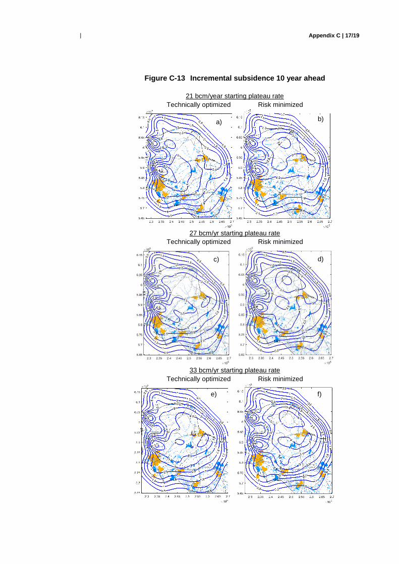
C.4.2 Observations The risked minimized pressure distribution generally shifts subsidence in north eastern direction. This effect is most pronounced in the 5 year ahead case (Figure C-11), while in the 10 year ahead case (Figure C-12) the effect diminishes. As Figure C-5 shows, after the next 10 to 15 year the Groningen field will enter a phase of relatively strong production decline. The flexibility to distribute production over de various production clusters is likely to strongly decrease during that phase.

Appendix C | 16/19
|
Figure C-12 Incremental subsidence 5 year ahead
21 bcm/year starting plateau rate Technically optimized Risk minimized
27 bcm/yr starting plateau rate
Technically optimized Risk minimized
33 bcm/yr starting plateau rate
Technically optimized Risk minimized
a) b)
c) d)
e) f)
Appendix C | 17/19
|
Figure C-13 Incremental subsidence 10 year ahead
21 bcm/year starting plateau rate Technically optimized Risk minimized
27 bcm/yr starting plateau rate
Technically optimized Risk minimized
33 bcm/yr starting plateau rate
Technically optimized Risk minimized
a) b)
c) d)
e) f)
Appendix C | 18/19
|
C.5 Findings
Compaction modelling
• The methodology for calculating compaction and subsidence has converged between NAM and TNO over the last few years. Both prefer the RTiCM compaction model and use inversion from subsidence data to constrain the model results.
• Through following independent workflows, NAM and TNO arrive at slightly
different RTiCM model parameters. These differences are likely to represent part of the uncertainty.
Subsidence forecasting
• TNO has independently calculated the long term subsidence evolution over the Groningen field. The results are in broad agreement with the results presented by NAM in WP2016.
• The impact of choosing a risk minimized pressure distribution is
pronounced for the next 5 years. It leads to a shift of compaction in northeastern direction. On the longer term (10 to 15 years+ from now) this effect is likely to diminish, in conjunction with a loss of flexibility of distributing production over clusters in the decline phase of the Groningen field production.
Appendix C | 19/19
|
References
NAM2016a Winningsplan Groningen Gasveld 2016 NAM 2016b Technical Addendum to the Winningsplan Groningen 2016:
Production, Subsidence, Induced Earthquakes and Seismic Hazard and Risk Assessment in the Groningen Field, Part I Summary & Production
NAM 2016c Technical Addendum to the Winningsplan Groningen 2016:
Production, Subsidence, Induced Earthquakes and Seismic Hazard and Risk Assessment in the Groningen Field, Part II Subsidence
TNO 2013 Toetsing van de bodemdalingsprognoses en seismische hazard ten
gevolge van gaswinning van het Groningen veld. TNO report 2013 R11953, 23 December 2013.
Fokker and VanThienen-Visser, 2016 Inversion of double difference
measurements from optical leveling for the Groningen gas field. International Journal of Applied Earth Observation and Geoinformation, 49, 1-9.
Pruiksma et al. 2015 Isotach formulation of the rate type compaction model for sandstone,
International Journal of Rock Mechanics and Mining Sciences, 78:127-132

Appendix D | 1/6
D Ground motion prediction equation (GMPE)
D.1 Introduction
D.1.1 General One of the major components of the seismic hazard and risk calculations for the production plan (WP 2016) Groningen Field 2016 is the ground motion prediction model. This is often referred to as the ground motion prediction equation or GMPE. This model provides the linking element between the seismological model (time, location and magnitudes of expected earthquakes) and the expected resulting ground motions at or near the free surface, where the motions are transferred to the built environment.
D.1.2 Documents The NAM developed a GMPE dedicated specifically to the Groningen field. Like the hazard and risk assessment as a whole, the development stages of the GMPE have been labeled with version numbers starting with V0, V1, etc. The current version under review has been documented and labeled with version number V2. This document will be referred to here as “ReportV2”. The earlier V1 version has been published and is referred to as “ReportV1”.
D.2 Review findings
D.2.1 General ReportV2 provides a very thorough, in-depth documentation and motivation of the data analysis and modelling choices that form the basis of the V2 ground motion model. The report makes clear, that the V2 version is a stage of a work in progress. Various improvements are planned and partly already in development (e.g. ReportV2, Chapter 13). The GMPE development as reported in ReportV1 and ReportV2 can be considered comprehensive and state-of-the-art. The authors are internationally recognized experts on the subject matter, and at various stages plans or results have been subjected to peer review from other recognized experts (see ReportV2, Acknowledgements). We limit our review to a number of critical model choices.
D.2.2 Application-specific GMPE
The choice to develop an application specific ground motion model for the Groningen field was motivated in ReportV1. The authors propose to do this more generally for cases of induced seismicity. In ReportV1 it is stated: “Because induced earthquakes are generally of smaller magnitude and shallower focal depth than the ranges typically covered by GMPEs derived for tectonic seismicity, the resulting ground motions are more likely to exhibit differences from
Appendix D | 2/6
one location or region to another than may be the case for natural earthquakes by virtue of sensitivity to the heterogeneous nature of the upper crust.” In addition, they state that “Given the nature of the projects causing induced seismicity, it is not uncommon to have a relatively detailed level of understanding of this upper-crustal structure”. In Groningen, this is obviously the case. ReportV2 testifies that this detailed understanding is taken into account in the Groningen GMPE. A general disadvantage of developing an application specific ground motion model for Groningen is the lack of data available for the range of magnitudes that contributes most to the hazard and risk. In the Groningen case, the main contribution to the risk seems to come from earthquakes above magnitude 4, which have not been observed in Groningen. While the ground motion model is calibrated on actual ground motions and source parameters observed in the field, the extrapolation to higher magnitudes relies on models rather than empirical data. The extrapolation is done using stochastic modelling of ground motions based on the Brune point source model. The parameters for this model are derived from the Groningen dataset. To correct for the finite dimensions of larger earthquakes, provisions are being made in both the geometrical spreading and the uncertainty model.
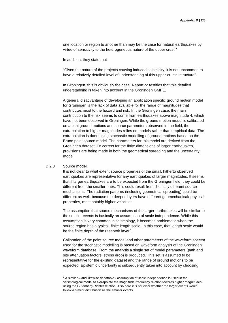
D.2.3 Source model It is not clear to what extent source properties of the small, hitherto observed earthquakes are representative for any earthquakes of larger magnitudes. It seems that if larger earthquakes are to be expected from the Groningen field, they could be different from the smaller ones. This could result from distinctly different source mechanisms. The radiation patterns (including geometrical spreading) could be different as well, because the deeper layers have different geomechanical/-physical properties, most notably higher velocities.
The assumption that source mechanisms of the larger earthquakes will be similar to the smaller events is basically an assumption of scale independence. While this assumption is very common in seismology, it becomes problematic when the source region has a typical, finite length scale. In this case, that length scale would be the finite depth of the reservoir layer2.
Calibration of the point source model and other parameters of the waveform spectra used for the stochastic modelling is based on waveform analysis of the Groningen waveform database. From the analysis a single set of model parameters (path and site attenuation factors, stress drop) is produced. This set is assumed to be representative for the existing dataset and the range of ground motions to be expected. Epistemic uncertainty is subsequently taken into account by choosing
2 A similar – and likewise debatable - assumption of scale independence is used in the seismological model to extrapolate the magnitude-frequency relation towards higher magnitudes using the Gutenberg-Richter relation. Also here it is not clear whether the larger events would follow a similar distribution as the smaller events.

Appendix D | 3/6
three values of stress drop. All other variability is expected to be covered by the aleatoric uncertainty implemented in the ground motion model. It is unclear how robust the estimates of the spectrum parameters are. There could be trade-offs (covariances) or trends to take into account. Important trends could be for example the variation of stress drop with time, compaction, or magnitude.
D.2.4 Site response The most influential visual change in the ground motion model going from V1 to V2 has been the incorporation of site-specific site response. Another influential change, especially for the amplitudes of the ground motions, is the incorporation of non-linear effects of the soil response. For the part of the spectrum that is relevant to the vulnerability of most buildings in the region3, the non-linear effects effectively damp ground motions. As a result, the hazard and risk submitted with the production plan (WP 2016) have reduced drastically with respect to earlier estimates.
Damping effect of the soils – though anticipated by many experts – has not been observed in the Groningen case. In fact, it is not expected to be noticeable for the levels of ground motions that have been observed so far. Experiments to test and calibrate the degradation of soil strength due to large strains have not yet been performed or reported for typical Groningen soils. Therefore, the damping effects incurred so far by necessity depend on empirical relations based on other soils. It is clear that this is a source of uncertainty. Within the site response analysis reported in ReportV2, this uncertainty is only accounted for in a limited way. That is by enhancing the site-to-site variability in the ground motion model. There is currently no provision for possible epistemic biases.
The choice of a deep rock horizon as the reference level for the site response analysis4 is motivated as follows. Below this depth the subsurface may be considered more or less homogeneous and the rock/soil response below this depth should be more or less linear. At this reference level no ground motions are being recorded. Hence, to derive the ground motion prediction equations for the reference level, all ground motions measurements must first be translated down to the reference horizon. This step is done using a site response model, comparable to the one that is used later on to translate the reference rock ground motions back to the free surface. The two-way dependence on the site response model may in some cases be attractive due to the internal consistency. However, in other cases the inaccuracies may accumulate. Since the reference rock GMPEs depends on the site response model, if the latter for some reason need to be revised, also the former should be revisited.
Figures D-1 and D-2 illustrate the effect of the GMPEs on hazard assessments according to the KNMI 2015 hazard model update (Dost and Spetzler, 2015). The parameter settings in the hazard assessment are chosen so as to mimic those in the production plan (WP 2016). The figures illustrate the effects of the V2 GMPE relative to the V1 model and should not be interpreted out of this context: this implementation has not been tested rigorously. The figures show that the non-linear part of the site response provides a reduction of up to 50% for the highest ground
3 short periods 4 in the V2 this is NU_B

Appendix D | 4/6
motions near the center of the field. It also appears that the linearized V2 model already shows a reduction of 20-40 % relative to the results of V1. It is not clear what the cause of this reduction is. It may be related to a slight reduction in the aleatoric uncertainty (sigma model).
Figure D-1: Effects of the V2 GMPE (in [g] ) when applied to the KNMI seismic hazard model with parameter settings as indicated, mimicking the model choices used in the submitted production plan (WP 2016). Top left: the V2 result at the surface, including (non-linear) site effects. Top right: the equivalent figure for the V1 GMPE (with V2 logic tree weights). Bottom left: the V2 hazard map at NU_B. Bottom right: result of V2 GMPE at the surface with non-linear effects removed.
Appendix D | 5/6
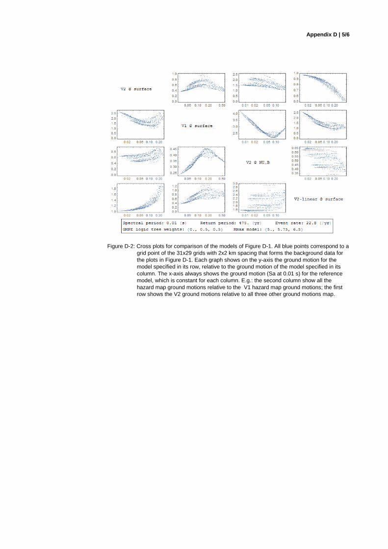
Figure D-2: Cross plots for comparison of the models of Figure D-1. All blue points correspond to a grid point of the 31x29 grids with 2x2 km spacing that forms the background data for the plots in Figure D-1. Each graph shows on the y-axis the ground motion for the model specified in its row, relative to the ground motion of the model specified in its column. The x-axis always shows the ground motion (Sa at 0.01 s) for the reference model, which is constant for each column. E.g.: the second column show all the hazard map ground motions relative to the V1 hazard map ground motions; the first row shows the V2 ground motions relative to all three other ground motions map.

Appendix D | 6/6
References
ReportV1 Developing an application-specific ground-motion model for
induced seismicity, Bommer et al., BSSA 106:1, February 2016.
ReportV2 Development of Version 2 GMPEs for Response Spectral
Accelerations and Significant Durations from Induced Earthquakes in the Groningen Field by Bommer et. al., November 2015
Dost and Spetzler, 2015 Probabilistic Seismic Hazard Analysis for Induced
Earthquakes in Groningen - update 2015. Report KNMI 2015.

Appendix D | 7/1
|