1

Sparse Multipath Wireless Channels: Modeling & Implications

Akbar M. Sayeed

ASAP 2006June 6-7, 2006

MIT Lincoln Labs

Wireless Communications LaboratoryElectrical and Computer Engineering

University of Wisconsin-Madison

akbar@engr.wisc.eduhttp://dune.ece.wisc.edu

2

Multipath Wireless Channels

• Multipath signal propagation over spatially distributed paths due to signal scattering from multiple objects – Necessitates statistical channel modeling– Accurate and analytically tractable Understanding the physics!

• Fading – fluctuations in received signal strength• Diversity – statistically independent modes of communication

3

Wideband Multi-Antenna RF Front-Ends• Communication in multiple dimensions

– Spatial dimension (antennas)– Spectral dimension (bandwidth)– Temporal dimensions (signaling duration/code length)– Redundant multipath sampling in angle-delay-Doppler

• High-dimensional, short “packet” codes– Low SNR/dimension– High coding efficiency (long “code lengths”)

• Agile RF front-ends– Reconfigurable antenna arrays– Frequency/bandwidth agility– Multi-resolution multipath sampling/imaging

• New theory for cognitive wireless communication and sensing– Physical channels get “sparse” in the wideband regime– Physical source-channel matching– Dramatic increase in capacity and reliability – Connections between wideband radar and communications

4

Overview

• Virtual channel modeling – Sparse multipath channels

• Implications of sparsity– Time-frequency coherence: channel learnability– New MIMO capacity scaling laws– Maximizing MIMO capacity with reconfigurable

arrays

5

Antenna Arrays: Multiplexing and Energy Capture

Multiplexing – Parallel spatial channels

sec/bitsW

1logW),W(C 2 ⎟⎠⎞

⎜⎝⎛ ρ+=ρ

( ) sec/bits1logNN

N1logN~),N(C 22 ρ+=⎟⎠⎞

⎜⎝⎛ ρ+ρ

Array aperture: Energy capture

Wideband (W):

Multi-antenna (N):

Dramatic linear increase in capacity with number of antennas

6

Wireless Channel Modeling

Spatial sampling commensurate with signal space resolution

Channel statistics induced by the physical scattering environment

Abstract statistical models(Foschini, Telatar)

Physical models(array processing)

Virtual Model

Tractable Accurate

Accurate & tractable

Interaction between the signal space and the physical channel

7

Narrowband MIMO Channel

Hsx =

⎥⎥⎥⎥⎥

⎦

⎤

⎢⎢⎢⎢⎢

⎣

⎡

⎥⎥⎥⎥

⎦

⎤

⎢⎢⎢⎢

⎣

⎡

=

⎥⎥⎥⎥⎥

⎦

⎤

⎢⎢⎢⎢⎢

⎣

⎡

TR NTRRR

T

T

N s

ss

NNHNHNH

NHHHNHHH

x

xx

2

1

2

1

),(,),2,(),1,(

),2(,),2,2(),1,2(),1(,),2,1(),1,1(

Received signal Transmitted signal

TN

RNTransmit antennas

Receive antennas

8

Uniform Linear Arrays

⎥⎥⎥⎥⎥

⎦

⎤

⎢⎢⎢⎢⎢

⎣

⎡

=θ

θ−π−

πθ−

RR

R

)1N(2j

2j

RR

e

e1

)(aReceive response veector

λφ=θ /)sin(d RRR

Receiver antenna spacing

Rd =

⎥⎥⎥⎥⎥

⎦

⎤

⎢⎢⎢⎢⎢

⎣

⎡

=θ

θ−π−

πθ−

TT

T

)1N(2j

2j

TT

e

e1

)(aTransmit steeringvector

λφ=θ /)sin(d TTT

Transmitter antenna spacing

Td =

2/2/ π≤φ≤π−

Spatial sinusoids: angles frequencies

φ5.05.0,/)sin(d ≤θ≤−λφ=θ

9

Physical Modeling of Narrowband MIMO Channels

)()( n,THTn,RR

N

1nn

path

θθβ= ∑=

aaH

pathN

}{ n,Rθ }{ n,Tθ

}{ nβ: number of paths : complex path gains

: Angles of Arrival (AoA’s) : Angles of Departure (AoD’s)

Non-linear dependence of H on AoA’s and AoD’s

10

Virtual MIMO Modeling

( ) )N/k(N/i)k,i(H)()( T

N

1i

N

1k

HTRRVn,T

N

1n

HTn,RRn

R Tpath

∑∑∑= ==

=θθβ= aaaaH

RRTT N/1,N/1 =θΔ=θΔSpatial array resolutions:

Physical Model Virtual Model

(AS 2002)

Virtual model is linear -- virtual beam angles are fixed

11

Computation of Virtual MIMO MatrixHTVR AHAH = T

HRV HAAH =

matrixDFTunitaryNN: RRR ×A

matrixDFTunitaryNN: TTT ×A

Two-dimensional unitary (Fourier) transform

Generalizable to non-ULA’s

Kotecha & AS (2004); Tulino, Lozano, Verdu (2005); Bonek 2004

[ ] HRRR

HR E AΛAHHΣ ≈= [ ] H

TTTH

T E AΛAHHΣ ≈=

12

Communication in Virtual/Eigen SpacensAHAnHsx +=+= H

TVR

VVVV nsHx +=⇒xAxsAsHRV

VT

=

=

MultipathPropagationEnvironmentTA

VsHRA

x Vx

is an image of the far-field of the RX

VxImage of is created in the far-field of TX

Vs

s

13

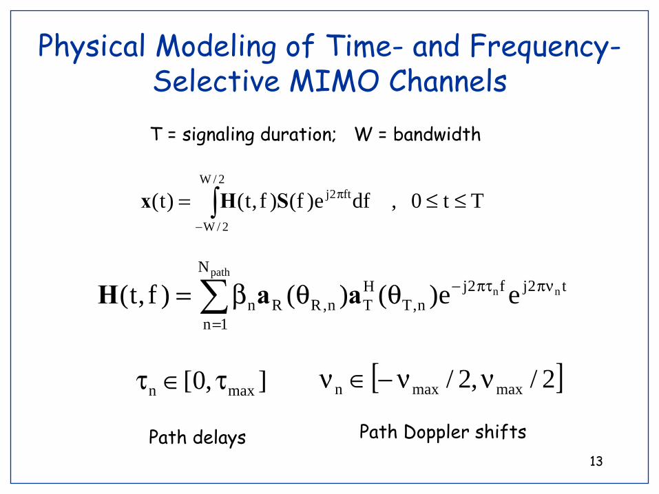
Physical Modeling of Time- and Frequency-Selective MIMO Channels

Tt0,dfe)f()f,t()t(2/W

2/W

ft2j ≤≤= ∫−

πSHx

t2jf2jn,T

HTn,RR

N

1nn

nn

path

ee)()()f,t( πνπτ−

=

θθβ= ∑ aaH

T = signaling duration; W = bandwidth

],0[ maxn τ∈τ [ ]2/,2/ maxmaxn νν−∈ν

Path delays Path Doppler shifts

14

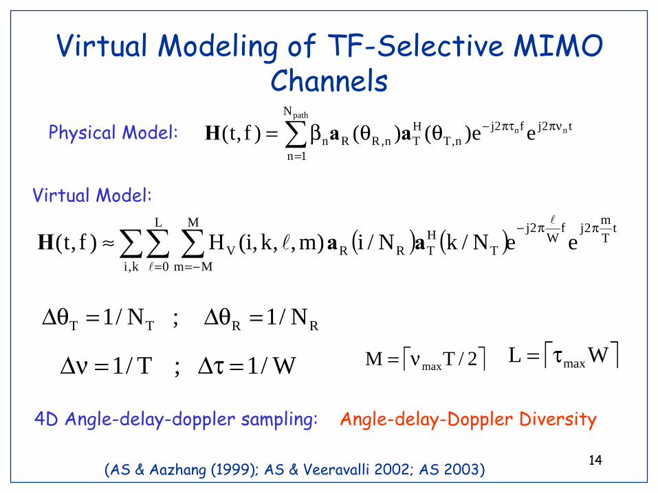
Virtual Modeling of TF-Selective MIMO Channels

t2jf2jn,T

HTn,RR

N

1nn

nn

path

ee)()()f,t( πνπτ−

=

θθβ= ∑ aaHPhysical Model:

RRTT N/1;N/1 =θΔ=θΔ

W/1;T/1 =τΔ=νΔ

( ) ( ) tTm2jf

W2j

k,iT

HTRR

L

0

M

MmV eeN/kN/i)m,,k,i(H)f,t(

ππ−

= −=∑∑ ∑≈ aaH

Virtual Model:

4D Angle-delay-doppler sampling:

(AS & Aazhang (1999); AS & Veeravalli 2002; AS 2003)

Angle-delay-Doppler Diversity

⎡ ⎤WL maxτ=⎡ ⎤2/TM maxν=

15

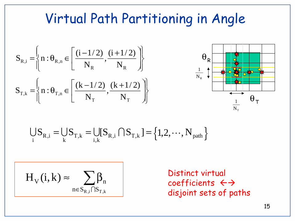
Virtual Path Partitioning in Angle

{ }pathk,Ti,Rk,i

k,Tk

i,Ri

N,,2,1]SS[SS ∩∪∪∪ ===

Tθ

Rθ⎪⎭

⎪⎬⎫

⎪⎩

⎪⎨⎧

⎟⎟⎠

⎞+⎢⎣

⎡ −∈θ=RR

n,Ri,R N)2/1i(,

N)2/1i(:nS

RN1

∑∈

β≈k,Ti,R SSnnV )k,i(H

∩

Distinct virtual coefficients disjoint sets of paths

TN1⎪⎭

⎪⎬⎫

⎪⎩

⎪⎨⎧

⎟⎟⎠

⎞+⎢⎣

⎡ −∈θ=TT

n,Tk,T N)2/1k(,

N)2/1k(:nS

16

τ

ν

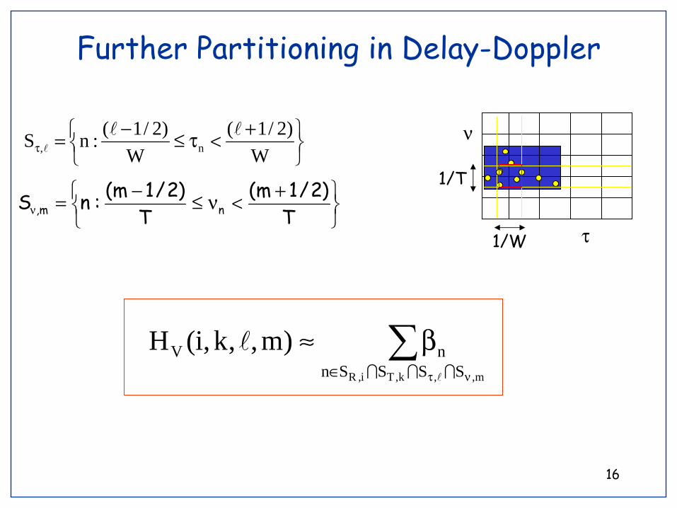
Further Partitioning in Delay-Doppler

1/W

⎭⎬⎫

⎩⎨⎧ +<τ≤−=τ W

)2/1(W

)2/1(:nS n,

⎭⎬⎫

⎩⎨⎧ +<ν≤−=ν T

)2/1m(T

)2/1m(:nS nm,

1/T

∑ντ∈

β≈m,,k,Ti,R SSSSn

nV )m,,k,i(H∩∩∩

17

Degrees of FreedomVirtual channel coefficients are approximately independent

[ ] 'mm''kk'ii*VV )m,,k,i()'m,','k,'i(H)m,,k,i(HE −−−− δδδδΨ≈

∑ντ∈

β≈m,,k,Ti,R SSSSn

nV )m,,k,i(H∩∩∩

( ) [ ] [ ]∑ντ∈

β≈=Ψm,,k,Ti,R SSSSn

2n

2V E)m,,k,i(HEm,,k,i

∩∩∩

⇓

Dominant (large power) virtual coefficients

Statistically independent Degrees of Freedom (DoF)

DoF’s are ultimately limited by the number of resolvable paths

18

Rich versus Sparse Multipath

Deg

rees

of

Free

dom

(D)

Rich (linear)

Sparse (sub-linear)

Signal Space Dimensions ( )sN

( ) maxmaxTRsmaxrich TWNNNODD ντ≈==

TWNNN TRs =Signal space dimensions:

( ) ( ) ( ) ]1,0[,;TWNNNoD maxmaxTRssparse ∈δγντ== δγ

19

Sparsity and Coherence• Spectral efficiency in the wideband regime (Verdu)

– Wide gap between coherent and non-coherent regimes – Flashy signaling

• Role of channel coherence (Medard, Tse, Zheng)– Channel learning– Non-flashy signaling

• Channel sparsity and coherence (Raghavan, Hariharan, AS)– Sparsity in angle-delay-Doppler coherence in space,

frequency, time– Channel coherence increases with bandwidth, signaling duration

and antennas– Important implications for wideband/low-SNR regime

20

Sparsity in Delay-Doppler

)t(weW

ts)m,(H)t(xm,

tTm2j

v +⎟⎠⎞

⎜⎝⎛ −=∑

π

( ) ( ) ]1,0[,N~TWD smaxmax ∈δντ= δδDelay-Doppler Diversity:

maxτ

2maxν−

2maxν

21

Time-Frequency Coherence Subspaces

DNTWN cs ==

Orthogonal Short-Time Fourier Signaling(Liu, Kadous, AS 2004)

STF basis functions:approx. Eigenfunctions for

underspread channels

δ

δ−

δ

δ−

ντ===

max

1

max

1

cohcohcWTWT

DTWN

D coherence subspaces (delay-Doppler diversity)

Dimension of each coherence subspace

( ) ( )δδντ= smaxmax N~TWD

22

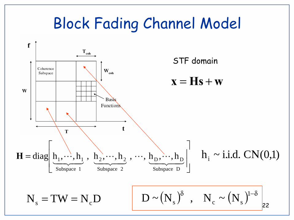
Block Fading Channel Model

⎥⎥

⎦

⎤

⎢⎢

⎣

⎡=

DSubspace

DD

2Subspace

22

1Subspace

11 h,,h,,h,,h,h,,hdiagH

wHsx +=

DNTWN cs ==

STF domain

)1,0(C.d.i.i~hi Ν

( ) ( ) δ−δ 1scs N~N,N~D

23

Channel Learning Via Training

WPSNR =SNRN

DPTE ctr η=η=

D,,1i,E11]|hh[|EMSE

tr

2ii =

+=−=

Use 1 signal space dimension in each coherence subspace for training

:)1,0(∈η Fraction of energy used for training

Training Energy per Coherence Subspace :

∞→⇔→ trE0MSE

P=total power

24

Sparse Channels are Asymptotically Coherent (Perfectly Estimatable)

0and0SEM →η→ ∗

In the limit of large signal space dimensions (T and W)

1,SNR

1~Nifonlyandif c >μμ

Maximizing mutual information (capacity) or the error exponent

(reliability)

Sparse channels:

Rich channels:

( )1<δ

( )1=δ

0SNRSNRN1~ 2

1

c

→=η−μ

∗

∞→=η −μ∗

21ctr

SNR

1SNRN~E

21and1SEM →η→ ∗

δ−δ>αα

1,W~T

(Hariharan and AS 2006)

25

Numerical Illustration

26

Sparse Narrowband MIMO Channels

• Sparsity in virtual (beam) domain correlation/coherence in the antenna (spatial) domain

• Optimal capacity: spatial distribution of the D(N) channel DoF in the possible channel dimensions (“resolution bins”)

)2,0(,N~)N(D ∈γγ

2N

NNN RT ==

27

MIMO Capacity Scaling

)N,Nmin( RT

CCorrelated channels (kronecker model)Chua et. al. ’02

i.i.d. modelTelatar ’95Foschini ’96 Physical channels

(virtual representation)Liu et. al. ’03

28

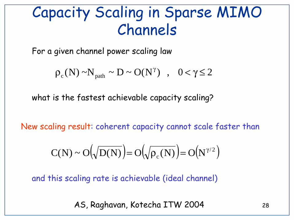
Capacity Scaling in Sparse MIMO Channels

20,)N(O~D~N~)N( pathc ≤γ<ρ γ

For a given channel power scaling law

what is the fastest achievable capacity scaling?

New scaling result: coherent capacity cannot scale faster than

( ) ( ) ( )2/c NO)N(O)N(DO~)N(C γ=ρ=

and this scaling rate is achievable (ideal channel)

AS, Raghavan, Kotecha ITW 2004

29

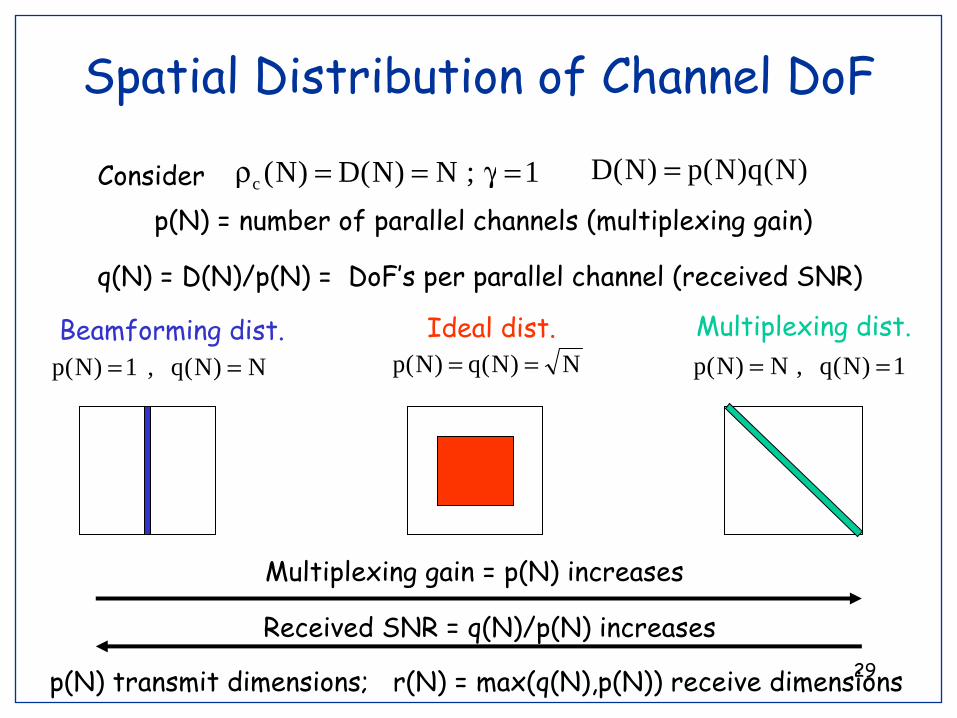
Spatial Distribution of Channel DoF

1;N)N(D)N(c =γ==ρ

Beamforming dist.

p(N) = number of parallel channels (multiplexing gain)

q(N) = D(N)/p(N) = DoF’s per parallel channel (received SNR)

Ideal dist.N)N(q)N(p ==N)N(q,1)N(p ==

Multiplexing dist.1)N(q,N)N(p ==

)N(q)N(p)N(D =Consider

p(N) transmit dimensions; r(N) = max(q(N),p(N)) receive dimensions

Multiplexing gain = p(N) increases

Received SNR = q(N)/p(N) increases

30

Capacity as a Function of SNR (fixed N)

⎟⎟⎠

⎞⎜⎜⎝

⎛ρ+=⎟⎟

⎠

⎞⎜⎜⎝

⎛ρ+≈ 2p

D1logppq1logpC

C(N

)

Beamforming:

Ideal:

Multiplexing:

Nq,1p ==

Nqp ==

1q,Np ==

NpqD ==

α= Np

31

Adaptive-resolution Spatial SignalingIdeal

Medium resolution TX and RX

Multiplexing gain and spatial coherence: Fewer independent streams with wider beamwidths at lower SNRs.

High resolution TX and RX

Multiplexing Beamforming

Low resolutionTXand High-Res. RX

32

Wideband/Low-SNR Capacity Limit

MUXmin,o

b

IDEALmin,o

b

BFmin,o

b

NE

N1

NE

N1

NE

⎟⎟⎠

⎞⎜⎜⎝

⎛=⎟⎟

⎠

⎞⎜⎜⎝

⎛=⎟⎟

⎠

⎞⎜⎜⎝

⎛

N-fold increase in capacity (or reduction in ) via beamforming configuration

minob )N/E(

33

Concluding Thoughts• Emerging wireless landscape

– Multitude of heterogeneous distributed devices– Agile RF front-ends

• Physics of communication– Multipath: a key resource – Dependencies in spatial, spectral, temporal dimensions

• Finite energy “packet” communication– High-dimensions– Agile RF-front ends: physical source-channel matching– New rate-reliability-energy tradeoff

• Integrated wireless communications and sensing– Connections with wideband radar– Cognitive wireless systems

http://dune.ece.wisc.edu

34

Quadratic Channel Power Scaling?)N(O~D~N 2

path is physically impossible indefinitely(received power < transmit power)

N

Total TX power

Total RX powerQuadratic growth in channel power

Linear growth in total received power

Linear capacity scaling

Increasing power coupling between the TX and RX due to increasing array apertures

[ ]2TX EP s=ρ= [ ] NP

NDPEP TXTX

2RX === sH

35

Channel Power and Degrees of Freedom

∑=

β===ρpathN

1n

2nV

HV

Hc ]|[|E])[E(trace])[E(trace)N( HHHH

( ) ( )pathc NO~DO~)N(ρ

Channel power:

Prevalent channel power normalization: )N(O~ 2cρ

)N(O~D~N 2path⇒

The number of paths/channel DoF grow quadratically with N

36

MIMO Channel Capacity

( )[ ] ( )[ ]HVVV)(tr

H)(tr detlogEmaxdetlogEmaxC

VHQHIHQHI QQ +=+= ρ≤ρ≤

nHsx +=

HToptTopt

opt,V

UΛUQQ

=

Optimal input covariance matrix is diagonal in the virtual domain:- beamforming optimal at low SNR (rank-1 input)- uniform power input optimal at high SNR (full-rank input)

[ ]2H E,][E sInn =ρ=

Veeravalli, Liang, AS (2003); Kotecha and AS (2003); Tulino, Lozano, Verdu (2003)

][E HssQ =

37

Ideal Channel: Optimum Capacity Scaling

[ ] α−γρ=ρ==ρ 22

rx N)N(p)N(q

)N(pE)N( Hs Received SNR per parallel channel

( ) ( )α−γα ρ+=ρ+≈ 2rx N1logN)N(1log)N(p)N(C

C(N

)

N

Beamforming:

Ideal:

20 ≤γ<10 ≤α≤

Multiplexing:

∞→ρ=ρρ+

N)N()N1log(~)N(C

rx

bf

ρ=ρρ+

)N()1log(N~)N(C

rx

id

0N/)N()N/1log(N~)N(C

rx

mux

→ρ=ρρ→ρ+

38

New Capacity Formulation for Reconfigurable Arrays

[ ])det(logEmaxmaxC HVVVpqD:)(tr VV

HQHIHQ

+==ρ≤

Maximization over channels (DoF distribution) not needed at high SNR

Very significant impact at low SNR

Optimal channel configuration realizable with reconfigurable antenna arrays

Sayeed and Raghavan 2004, 2006

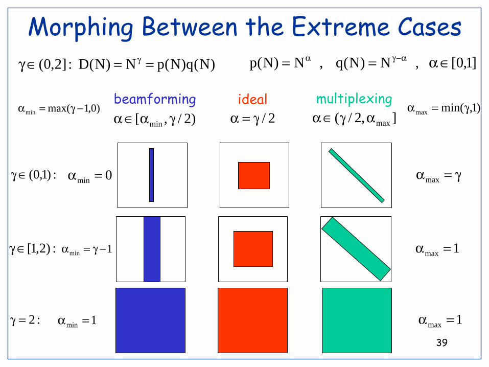
39

Morphing Between the Extreme Cases)N(q)N(pN)N(D:]2,0( ==∈γ γ

:)1,0(∈γ

:)2,1[∈γ

0min =α

1min −γ=α

beamforming)2/,[ min γα∈α

ideal2/γ=α

multiplexing],2/( maxαγ∈α

)0,1max(min −γ=α )1,min(max γ=α

]1,0[,N)N(q,N)N(p ∈α== α−γα

γ=αmax

1max =α

:2=γ 1min =α 1max =α

40

Angle-Delay-Doppler Sampling

1/Q

1/P Tθ

Rθ

1/W

1/T

τ

ν

Spatial degrees of freedom)1Q~2)(1P~2(NS ++=

Temporal and spectral degrees of freedom

)1M2)(1L(NT ++=

41

Virtual Path Partitioning

{ }path

l,m,p,Tq,Rl,m,p,q

l,lm,

mp,Tpq,R

q

N,,2,1

]SSSS[

SSSS

∩∩∩∪

∪∪∪∪

=

=

===

τν

τν

Tθ

Rθ

τ

ν

1/W

⎭⎬⎫

⎩⎨⎧ +<τ≤−=τ W

)2/1l(W

)2/1l(:nS nl,

1/Q⎭⎬⎫

⎩⎨⎧ +<θ≤−=

Q)2/1q(

Q)2/1q(:nS n,Rq,R

1/P⎭⎬⎫

⎩⎨⎧ +

<θ≤−

=P

)2/1p(P

)2/1p(:nS n,Tp,T

⎭⎬⎫

⎩⎨⎧ +<ν≤−=ν T

)2/1m(T

)2/1m(:nS nm,

1/T

∑τν∈

β≈l,m,p,Tq,R SSSSn

nV ]l,m;p,q[H∩∩∩

42