155141903 Slicing a New Approach for Privacy Preserving Data Publishing

Slicing: A New Approach forPrivacy Preserving Data Publishing

Tiancheng Li, Ninghui Li, Senior Member, IEEE, Jian Zhang, Member, IEEE, and Ian Molloy

Abstract—Several anonymization techniques, such as generalization and bucketization, have been designed for privacy preserving

microdata publishing. Recent work has shown that generalization loses considerable amount of information, especially for high-

dimensional data. Bucketization, on the other hand, does not prevent membership disclosure and does not apply for data that do not

have a clear separation between quasi-identifying attributes and sensitive attributes. In this paper, we present a novel technique called

slicing, which partitions the data both horizontally and vertically. We show that slicing preserves better data utility than generalization

and can be used for membership disclosure protection. Another important advantage of slicing is that it can handle high-dimensional

data. We show how slicing can be used for attribute disclosure protection and develop an efficient algorithm for computing the sliced

data that obey the ‘-diversity requirement. Our workload experiments confirm that slicing preserves better utility than generalization

and is more effective than bucketization in workloads involving the sensitive attribute. Our experiments also demonstrate that slicing

can be used to prevent membership disclosure.

Index Terms—Privacy preservation, data anonymization, data publishing, data security.

Ç

1 INTRODUCTION

PRIVACY-PRESERVING publishing of microdata has beenstudied extensively in recent years. Microdata contains

records each of which contains information about anindividual entity, such as a person, a household, or anorganization. Several microdata anonymization techniqueshave been proposed. The most popular ones are general-ization [28], [30] for k-anonymity [30] and bucketization[34], [26], [17] for ‘-diversity [25]. In both approaches,attributes are partitioned into three categories: 1) someattributes are identifiers that can uniquely identify anindividual, such as Name or Social Security Number; 2) someattributes are Quasi Identifiers (QI), which the adversary mayalready know (possibly from other publicly availabledatabases) and which, when taken together, can potentiallyidentify an individual, e.g., Birthdate, Sex, and Zipcode;3) some attributes are Sensitive Attributes (SAs), which areunknown to the adversary and are considered sensitive,such as Disease and Salary.

In both generalization and bucketization, one firstremoves identifiers from the data and then partitions tuplesinto buckets. The two techniques differ in the next step.Generalization transforms the QI-values in each bucket into“less specific but semantically consistent” values so thattuples in the same bucket cannot be distinguished by theirQI values. In bucketization, one separates the SAs from theQIs by randomly permuting the SA values in each bucket.

The anonymized data consist of a set of buckets withpermuted sensitive attribute values.

1.1 Motivation of Slicing

It has been shown [1], [16], [34] that generalization for k-anonymity losses considerable amount of information,especially for high-dimensional data. This is due to thefollowing three reasons. First, generalization for k-anon-ymity suffers from the curse of dimensionality. In order forgeneralization to be effective, records in the same bucketmust be close to each other so that generalizing the recordswould not lose too much information. However, in high-dimensional data, most data points have similar distanceswith each other, forcing a great amount of generalizationto satisfy k-anonymity even for relatively small k’s. Second,in order to perform data analysis or data mining tasks onthe generalized table, the data analyst has to make theuniform distribution assumption that every value in ageneralized interval/set is equally possible, as no otherdistribution assumption can be justified. This significantlyreduces the data utility of the generalized data. Third,because each attribute is generalized separately, correla-tions between different attributes are lost. In order to studyattribute correlations on the generalized table, the dataanalyst has to assume that every possible combination ofattribute values is equally possible. This is an inherentproblem of generalization that prevents effective analysisof attribute correlations.

While bucketization [34], [26], [17] has better data utilitythan generalization, it has several limitations. First, buck-etization does not prevent membership disclosure [27].Because bucketization publishes the QI values in theiroriginal forms, an adversary can find out whether anindividual has a record in the published data or not. Asshown in [30], 87 percent of the individuals in the UnitedStates can be uniquely identified using only three attributes(Birthdate, Sex, and Zipcode). A microdata (e.g., census data)

IEEE TRANSACTIONS ON KNOWLEDGE AND DATA ENGINEERING, VOL. 24, NO. 3, MARCH 2012 561

. T. Li, N. Li, and I. Molloy are with the Department of Computer Science,Purdue University, West Lafayette, IN 47907.E-mail: {li83, ninghui, imolloy}@cs.purdue.edu.

. J. Zhang is with the Department of Statistics, Purdue University, WestLafayette, IN 47907. E-mail: [email protected].

Manuscript received 17 Feb. 2010; revised 26 Apr. 2010; accepted 19 July2010; published online 18 Nov. 2010.Recommended for acceptance by E. Ferrari.For information on obtaining reprints of this article, please send e-mail to:[email protected], and reference IEEECS Log Number TKDE-2010-02-0097.Digital Object Identifier no. 10.1109/TKDE.2010.236.

1041-4347/12/$31.00 � 2012 IEEE Published by the IEEE Computer Society

usually contains many other attributes besides those threeattributes. This means that the membership information ofmost individuals can be inferred from the bucketized table.Second, bucketization requires a clear separation betweenQIs and SAs. However, in many data sets, it is unclearwhich attributes are QIs and which are SAs. Third, byseparating the sensitive attribute from the QI attributes,bucketization breaks the attribute correlations between theQIs and the SAs.

In this paper, we introduce a novel data anonymizationtechnique called slicing to improve the current state of theart. Slicing partitions the data set both vertically andhorizontally. Vertical partitioning is done by groupingattributes into columns based on the correlations among theattributes. Each column contains a subset of attributes thatare highly correlated. Horizontal partitioning is done bygrouping tuples into buckets. Finally, within each bucket,values in each column are randomly permutated (or sorted)to break the linking between different columns.

The basic idea of slicing is to break the association crosscolumns, but to preserve the association within eachcolumn. This reduces the dimensionality of the data andpreserves better utility than generalization and bucketiza-tion. Slicing preserves utility because it groups highlycorrelated attributes together, and preserves the correla-tions between such attributes. Slicing protects privacybecause it breaks the associations between uncorrelatedattributes, which are infrequent and thus identifying. Notethat when the data set contains QIs and one SA, bucketiza-tion has to break their correlation; slicing, on the otherhand, can group some QI attributes with the SA, preservingattribute correlations with the sensitive attribute.

The key intuition that slicing provides privacy protectionis that the slicing process ensures that for any tuple, thereare generally multiple matching buckets. Given a tuplet ¼ v1; v2; . . . ; vch i, where c is the number of columns and viis the value for the ith column, a bucket is a matchingbucket for t if and only if for each i (1 � i � c), vi appears atleast once in the i’th column of the bucket. Any bucket thatcontains the original tuple is a matching bucket. At thesame time, a matching bucket can be due to containingother tuples each of which contains some but not all vi’s.

1.2 Contributions & Organization

In this paper, we present a novel technique called slicing forprivacy-preserving data publishing. Our contributionsinclude the following.

First, we introduce slicing as a new technique for privacypreserving data publishing. Slicing has several advantageswhen compared with generalization and bucketization. Itpreserves better data utility than generalization. It preservesmore attribute correlations with the SAs than bucketization.It can also handle high-dimensional data and data without aclear separation of QIs and SAs.

Second, we show that slicing can be effectively used forpreventing attribute disclosure, based on the privacyrequirement of ‘-diversity. We introduce a notion called ‘-diverse slicing, which ensures that the adversary cannotlearn the sensitive value of any individual with a probabilitygreater than 1=‘.

Third, we develop an efficient algorithm for computingthe sliced table that satisfies ‘-diversity. Our algorithmpartitions attributes into columns, applies column general-ization, and partitions tuples into buckets. Attributes that arehighly correlated are in the same column; this preserves thecorrelations between such attributes. The associations be-tween uncorrelated attributes are broken; this provides betterprivacy as the associations between such attributes are less-frequent and potentially identifying.

Fourth, we describe the intuition behind membershipdisclosure and explain how slicing prevents membershipdisclosure. A bucket of size k can potentially matchkc tuples where c is the number of columns. Because onlyk of the kc tuples are actually in the original data, theexistence of the other kc � k tuples hides the membershipinformation of tuples in the original data.

Finally, we conduct extensive workload experiments. Ourresults confirm that slicing preserves much better data utilitythan generalization. In workloads involving the sensitiveattribute, slicing is also more effective than bucketization.Our experiments also show the limitations of bucketizationin membership disclosure protection and slicing remediesthese limitations. We also evaluated the performance ofslicing in anonymizing the Netflix Prize data set.

The rest of this paper is organized as follows: InSection 2, we formalize the slicing technique and compareit with generalization and bucketization. We define‘-diverse slicing for attribute disclosure protection inSection 3 and develop an efficient algorithm to achieve‘-diverse slicing in Section 4. In Section 5, we explain howslicing prevents membership disclosure. In Section 6, wepresent an extensive experimental study on slicing and inSection 7, we evaluate the performance of slicing inanonymizing the Netflix Prize data set. We discuss relatedwork in Section 8 and conclude the paper and discussfuture research in Section 9.

2 SLICING

In this section, we first give an example to illustrate slicing.We then formalize slicing, compare it with generalizationand bucketization, and discuss privacy threats that slicingcan address.

Table 1 shows an example microdata table and itsanonymized versions using various anonymization techni-ques. The original table is shown in Table 1a. The three QIattributes are fAge; Sex; Zipcodeg, and the sensitive attri-bute SA is Disease. A generalized table that satisfies 4-anonymity is shown in Table 1b, a bucketized table thatsatisfies 2-diversity is shown in Table 1c, a generalized tablewhere each attribute value is replaced with the multiset ofvalues in the bucket is shown in Table 1d, and two slicedtables are shown in Tables 1e and 1f.

Slicing first partitions attributes into columns. Eachcolumn contains a subset of attributes. This verticallypartitions the table. For example, the sliced table in Table 1fcontains two columns: the first column contains fAge; Sexgand the second column contains fZipcode; Diseaseg. Thesliced table shown in Table 1e contains four columns, whereeach column contains exactly one attribute.

Slicing also partition tuples into buckets. Each bucketcontains a subset of tuples. This horizontally partitions the

562 IEEE TRANSACTIONS ON KNOWLEDGE AND DATA ENGINEERING, VOL. 24, NO. 3, MARCH 2012

table. For example, both sliced tables in Tables 1e and 1fcontain two buckets, each containing four tuples.

Within each bucket, values in each column are randomlypermutated to break the linking between different columns.For example, in the first bucket of the sliced table shown inTable 1f, the values fð22;MÞ; ð22; F Þ; ð33; F Þ; ð52; F Þg arerandomly permutated and the values fð47906; dyspepsiaÞ,ð47906; fluÞ,ð47905; fluÞ, ð47905; bronchitisÞg are randomlypermutated so that the linking between the two columnswithin one bucket is hidden.

2.1 Formalization of Slicing

Let T be the microdata table to be published. T containsd attributes: A ¼ fA1; A2; . . . ; Adg and their attribute do-mains are fD½A1�; D½A2�; . . . ; D½Ad�g. A tuple t 2 T can berepresented as t ¼ ðt½A1�; t½A2�; . . . ; t½Ad�Þ where t½Ai� ð1 �i � dÞ is the Ai value of t.

Definition 1 (Attribute Partition and Columns). An

attribute partition consists of several subsets of A, suchthat each attribute belongs to exactly one subset. Each subset of

attributes is called a column. Specifically, let there be c

columns C1; C2; . . . ; Cc, then [ci¼1Ci ¼ A and for any

1 � i1 6¼ i2 � c, Ci1 \ Ci2 ¼ ;.

For simplicity of discussion, we consider only onesensitive attribute S. If the data contain multiple sensitiveattributes, one can either consider them separately orconsider their joint distribution [25]. Exactly one of thec columns contains S. Without loss of generality, let thecolumn that contains S be the last column Cc. This columnis also called the sensitive column. All other columnsfC1; C2; . . . ; Cc�1g contain only QI attributes.

Definition 2 (Tuple Partition and Buckets). A tuple

partition consists of several subsets of T , such that eachtuple belongs to exactly one subset. Each subset of tuples is

called a bucket. Specifically, let there be b buckets

B1; B2; . . . ; Bb, then [bi¼1Bi ¼ T and for any 1 � i1 6¼i2 � b, Bi1 \Bi2 ¼ ;.

Definition 3 (Slicing). Given a microdata table T , a slicing ofT is given by an attribute partition and a tuple partition.

For example, Tables 1e and 1f are two sliced tables. InTable 1e, the attribute partition is {{Age}, {Sex}, {Zipcode},{Disease}} and the tuple partition is {{t1; t2; t3; t4},{t5; t6; t7; t8}}. In Table 1f, the attribute partition is {{Age,Sex}, {Zipcode, Disease}} and the tuple partition is{{t1; t2; t3; t4}, {t5; t6; t7; t8}}.

Often times, slicing also involves column generalization.

Definition 4 (Column Generalization). Given a microdatatable T and a column Ci ¼ fAi1; Ai2; . . . ; Aijg whereAi1; Ai2; . . . ; Aij are attributes, a column generalizationfor Ci is defined as a set of nonoverlapping j-dimensionalregions that completely cover D½Ai1� �D½Ai2� � � � � �D½Aij�. A column generalization maps each value of Ci tothe region in which the value is contained.

Column generalization ensures that one column satisfiesthe k-anonymity requirement. It is a multidimensionalencoding [19] and can be used as an additional step inslicing. Specifically, a general slicing algorithm consists ofthe following three phases: attribute partition, columngeneralization, and tuple partition. Because each columncontains much fewer attributes than the whole table,attribute partition enables slicing to handle high-dimen-sional data.

A key notion of slicing is that of matching buckets.

Definition 5 (Matching Buckets). Let fC1; C2; . . . ; Ccg be thec columns of a sliced table. Let t be a tuple, and t½Ci� be the Civalue of t. Let B be a bucket in the sliced table, and B½Ci� be themultiset of Ci values in B. We say that B is a matchingbucket of t iff for all 1 � i � c, t½Ci� 2 B½Ci�.

LI ET AL.: SLICING: A NEW APPROACH FOR PRIVACY PRESERVING DATA PUBLISHING 563

TABLE 1An Original Microdata Table and Its Anonymized Versions Using Various Anonymization Techniques

(a) The original table, (b) the generalized table, (c) the bucketized table, (d) multiset-based generalization, (e) one-attribute-per-column slicing, (f) thesliced table.

For example, consider the sliced table shown in Table 1f,and consider t1 ¼ ð22;M; 47906; dyspepsiaÞ. Then, the set ofmatching buckets for t1 is fB1g.

2.2 Comparison with Generalization

There are several types of recodings for generalization. Therecoding that preserves the most information is localrecoding [36]. In local recoding, one first groups tuples intobuckets and then for each bucket, one replaces all values ofone attribute with a generalized value. Such a recoding islocal because the same attribute value may be generalizeddifferently when they appear in different buckets.

We now show that slicing preserves more informationthan such a local recoding approach, assuming that thesame tuple partition is used. We achieve this by showingthat slicing is better than the following enhancement of thelocal recoding approach. Rather than using a generalizedvalue to replace more specific attribute values, one usesthe multiset of exact values in each bucket. For example,Table 1b is a generalized table, and Table 1d is the resultof using multisets of exact values rather than generalizedvalues. For the Age attribute of the first bucket, we use themultiset of exact values {22, 22, 33, 52} rather than thegeneralized interval [22-52]. The multiset of exact valuesprovides more information about the distribution of valuesin each attribute than the generalized interval. Therefore,using multisets of exact values preserves more informationthan generalization.

However, we observe that this multiset-based general-ization is equivalent to a trivial slicing scheme where eachcolumn contains exactly one attribute, because bothapproaches preserve the exact values in each attribute butbreak the association between them within one bucket. Forexample, Table 1e is equivalent to Table 1d. Now comparingTable 1e with the sliced table shown in Table 1f, we observethat while one-attribute-per-column slicing preserves attri-bute distributional information, it does not preserveattribute correlation, because each attribute is in its owncolumn. In slicing, one groups correlated attributes togetherin one column and preserves their correlation. For example,in the sliced table shown in Table 1f, correlations betweenAge and Sex and correlations between Zipcode and Diseaseare preserved. In fact, the sliced table encodes the sameamount of information as the original data with regard tocorrelations between attributes in the same column.

Another important advantage of slicing is its ability tohandle high-dimensional data. By partitioning attributesinto columns, slicing reduces the dimensionality of the data.Each column of the table can be viewed as a subtable with alower dimensionality. Slicing is also different from theapproach of publishing multiple independent subtables [16]in that these subtables are linked by the buckets in slicing.The idea of slicing is to achieve a better trade-off betweenprivacy and utility by preserving correlations betweenhighly correlated attributes and breaking correlationsbetween uncorrelated attributes.

2.3 Comparison with Bucketization

To compare slicing with bucketization, we first note thatbucketization can be viewed as a special case of slicing,where there are exactly two columns: one column contains

only the SA, and the other contains all the QIs. Theadvantages of slicing over bucketization can be understoodas follows: First, by partitioning attributes into more thantwo columns, slicing can be used to prevent membershipdisclosure. Our empirical evaluation on a real data setshows that bucketization does not prevent membershipdisclosure in Section 6.

Second, unlike bucketization, which requires a clearseparation of QI attributes and the sensitive attribute, slicingcan be used without such a separation. For data set such asthe census data, one often cannot clearly separate QIs fromSAs because there is no single external public database thatone can use to determine which attributes the adversaryalready knows. Slicing can be useful for such data.

Finally, by allowing a column to contain both some QIattributes and the sensitive attribute, attribute correlationsbetween the sensitive attribute and the QI attributes arepreserved. For example, in Table 1f, Zipcode and Diseaseform one column, enabling inferences about their correla-tions. Attribute correlations are important utility in datapublishing. For workloads that consider attributes inisolation, one can simply publish two tables, one containingall QI attributes and one containing the sensitive attribute.

2.4 Privacy Threats

When publishing microdata, there are three types ofprivacy disclosure threats. The first type is membershipdisclosure. When the data set to be published is selectedfrom a large population and the selection criteria aresensitive (e.g., only diabetes patients are selected), oneneeds to prevent adversaries from learning whether one’srecord is included in the published data set.

The second type is identity disclosure, which occurs whenan individual is linked to a particular record in the releasedtable. In some situations, one wants to protect againstidentity disclosure when the adversary is uncertain ofmembership. In this case, protection against membershipdisclosure helps protect against identity disclosure. In othersituations, some adversary may already know that anindividual’s record is in the published data set, in whichcase, membership disclosure protection either does notapply or is insufficient.

The third type is attribute disclosure, which occurs whennew information about some individuals is revealed, i.e.,the released data make it possible to infer the attributes ofan individual more accurately than it would be possiblebefore the release. Similar to the case of identity disclosure,we need to consider adversaries who already know themembership information. Identity disclosure leads toattribute disclosure. Once there is identity disclosure, anindividual is reidentified and the corresponding sensitivevalue is revealed. Attribute disclosure can occur with orwithout identity disclosure, e.g., when the sensitive valuesof all matching tuples are the same.

For slicing, we consider protection against membershipdisclosure and attribute disclosure. It is a little unclear howidentity disclosure should be defined for sliced data (or fordata anonymized by bucketization), since each tuple resideswithin a bucket and within the bucket the association acrossdifferent columns are hidden. In any case, because identitydisclosure leads to attribute disclosure, protection against


attribute disclosure is also sufficient protection againstidentity disclosure.

We would like to point out a nice property of slicing thatis important for privacy protection. In slicing, a tuple canpotentially match multiple buckets, i.e., each tuple can havemore than one matching buckets. This is different fromprevious work on generalization (global recoding specifi-cally) and bucketization, where each tuple can belong to aunique equivalence-class (or bucket). In fact, it has beenrecognized [3] that restricting a tuple in a unique buckethelps the adversary but does not improve data utility. Wewill see that allowing a tuple to match multiple buckets isimportant for both attribute disclosure protection andmembership disclosure protection, when we describe themin Sections 3 and 5, respectively.

3 ATTRIBUTE DISCLOSURE PROTECTION

In this section, we show how slicing can be used to preventattribute disclosure, based on the privacy requirement of‘-diversity and introduce the notion of ‘-diverse slicing.

3.1 Example

We first give an example illustrating how slicing satisfies‘-diversity [25] where the sensitive attribute is “Disease.”The sliced table shown in Table 1f satisfies 2-diversity.Consider tuple t1 with QI values ð22;M; 47906Þ. In order todetermine t1’s sensitive value, one has to examinet1’s matching buckets. By examining the first columnðAge; SexÞ in Table 1f, we know that t1 must be in the firstbucket B1 because there are no matches of ð22;MÞ inbucket B2. Therefore, one can conclude that t1 cannot be inbucket B2 and t1 must be in bucket B1.

Then, by examining the Zipcode attribute of the secondcolumn ðZipcode;DiseaseÞ in bucket B1, we know that thecolumn value for t1 must be either ð47906; dyspepsiaÞ orð47906; fluÞ because they are the only values that matcht1’s zipcode 47906. Note that the other two column valueshave zipcode 47905. Without additional knowledge, bothdyspepsia and flu are equally possible to be the sensitivevalue of t1. Therefore, the probability of learning the correctsensitive value of t1 is bounded by 0.5. Similarly, we canverify that 2-diversity is satisfied for all other tuples inTable 1f.

3.2 ‘-Diverse Slicing

In the above example, tuple t1 has only one matchingbucket. In general, a tuple t can have multiple matchingbuckets. We now extend the above analysis to the generalcase and introduce the notion of ‘-diverse slicing.

Consider an adversary who knows all the QI values of tand attempts to infer t’s sensitive value from the slicedtable. She or he first needs to determine which buckets tmay reside in, i.e., the set of matching buckets of t. Tuple tcan be in any one of its matching buckets. Let pðt; BÞ be theprobability that t is in bucket B (the procedure forcomputing pðt; BÞ will be described later in this section).For example, in the above example, pðt1; B1Þ ¼ 1 andpðt1; B2Þ ¼ 0.

In the second step, the adversary computes pðt; sÞ, theprobability that t takes a sensitive value s. pðt; sÞ is

calculated using the law of total probability. Specifically, letpðsjt; BÞ be the probability that t takes sensitive value s

given that t is in bucket B, then according to the law of totalprobability, the probability pðt; sÞ is

pðt; sÞ ¼X

B

pðt; BÞpðsjt; BÞ: ð1Þ

In the rest of this section, we show how to compute thetwo probabilities: pðt; BÞ and pðsjt; BÞ.

Computing pðt; BÞ. Given a tuple t and a sliced bucketB, the probability that t is in B depends on the fraction oft’s column values that match the column values in B. Ifsome column value of t does not appear in the correspond-ing column of B, it is certain that t is not in B. In general,bucket B can potentially match jBjc tuples, where jBj is thenumber of tuples in B. Without additional knowledge, onehas to assume that the column values are independent;therefore, each of the jBjc tuples is equally likely to be anoriginal tuple. The probability that t is in B depends on thefraction of the jBjc tuples that match t.

We formalize the above analysis. We consider the matchbetween t’s column values ft½C1�; t½C2�; . . . ; t½Cc�g andB’s column values fB½C1�; B½C2�; . . . ; B½Cc�g. Let fiðt; BÞð1 � i � c� 1Þ be the fraction of occurrences of t½Ci� in B½Ci�and let fcðt; BÞ be the fraction of occurrences of t½Cc � fSg�in B½Cc � fSg�Þ. Note that, Cc � fSg is the set of QIattributes in the sensitive column. For example, in Table1f, f1ðt1; B1Þ ¼ 1=4 ¼ 0:25 and f2ðt1; B1Þ ¼ 2=4 ¼ 0:5. Simi-larly, f1ðt1; B2Þ ¼ 0 and f2ðt1; B2Þ ¼ 0. Intuitively, fiðt; BÞmeasures the matching degree on column Ci, between tuple tand bucket B.

Because each possible candidate tuple is equally likely tobe an original tuple, the matching degree between t and B isthe product of the matching degree on each column, i.e.,fðt; BÞ ¼

Q1�i�c fiðt; BÞ. Note that

Pt fðt; BÞ ¼ 1 and when

B is not a matching bucket of t, fðt; BÞ ¼ 0.Tuple t may have multiple matching buckets, t’s total

matching degree in the whole data is fðtÞ ¼P

B fðt; BÞ. Theprobability that t is in bucket B is

pðt; BÞ ¼ fðt; BÞfðtÞ :

Computing pðsjt; BÞ. Suppose that t is in bucket B, todetermine t’s sensitive value, one needs to examine thesensitive column of bucket B. Since the sensitive columncontains the QI attributes, not all sensitive values can bet’s sensitive value. Only those sensitive values whose QIvalues match t’s QI values are t’s candidate sensitive values.Without additional knowledge, all candidate sensitivevalues (including duplicates) in a bucket are equallypossible. Let Dðt; BÞ be the distribution of t’s candidatesensitive values in bucket B.

Definition 6 (DDðt; BÞ). Any sensitive value that is associatedwith t½Cc � fSg� in B is a candidate sensitive value fort (there are fcðt; BÞ candidate sensitive values for t in B,including duplicates). Let Dðt; BÞ be the distribution of thecandidate sensitive values in B and Dðt; BÞ½s� be theprobability of the sensitive value s in the distribution.


For example, in Table 1f, Dðt1; B1Þ ¼ ðdyspepsia :

0:5; flu : 0:5Þ and therefore Dðt1; B1Þ½dyspepsia� ¼ 0:5. The

probability pðsjt; BÞ is exactly Dðt; BÞ½s�, i.e., pðsjt; BÞ ¼Dðt; BÞ½s�.‘-Diverse Slicing. Once we have computed pðt; BÞ and

pðsjt; BÞ, we are able to compute the probability pðt; sÞ basedon the (1). We can show when t is in the data, theprobabilities that t takes a sensitive value sum up to 1.

Fact 1. For any tuple t 2 D,P

s pðt; sÞ ¼ 1.

Proof.

X

s

pðt; sÞ ¼X

s

X

B

pðt; BÞpðsjt; BÞ

¼X

B

pðt; BÞX

s

pðsjt; BÞ

¼X

B

pðt; BÞ

¼ 1:

ð2Þ

tu‘-Diverse slicing is defined based on the probability

pðt; sÞ.Definition 7 (‘-diverse slicing). A tuple t satisfies ‘-diversity

iff for any sensitive value s

pðt; sÞ � 1=‘:

A sliced table satisfies ‘-diversity iff every tuple in it satisfies‘-diversity.

Our analysis above directly show that from an ‘-diversesliced table, an adversary cannot correctly learn thesensitive value of any individual with a probability greaterthan 1=‘. Note that once we have computed the probabilitythat a tuple takes a sensitive value, we can also use slicingfor other privacy measures such as t-closeness [21].

4 SLICING ALGORITHMS

We now present an efficient slicing algorithm to achieve‘-diverse slicing. Given a microdata table T and twoparameters c and ‘, the algorithm computes the sliced tablethat consists of c columns and satisfies the privacyrequirement of ‘-diversity.

Our algorithm consists of three phases: attribute partition-ing, column generalization, and tuple partitioning. We nowdescribe the three phases.

4.1 Attribute Partitioning

Our algorithm partitions attributes so that highly correlatedattributes are in the same column. This is good for bothutility and privacy. In terms of data utility, grouping highlycorrelated attributes preserves the correlations among thoseattributes. In terms of privacy, the association of uncorre-lated attributes presents higher identification risks than theassociation of highly correlated attributes because theassociation of uncorrelated attribute values is much lessfrequent and thus more identifiable. Therefore, it is better tobreak the associations between uncorrelated attributes, inorder to protect privacy.

In this phase, we first compute the correlations betweenpairs of attributes and then cluster attributes based on theircorrelations.

4.1.1 Measures of Correlation

Two widely used measures of association are Pearsoncorrelation coefficient [5] and mean-square contingencycoefficient [5]. Pearson correlation coefficient is used formeasuring correlations between two continuous attributeswhile mean-square contingency coefficient is a chi-squaremeasure of correlation between two categorical attributes.We choose to use the mean-square contingency coefficientbecause most of our attributes are categorical. Given twoattributes A1 and A2 with domains fv11; v12; . . . ; v1d1

g andfv21; v22; . . . ; v2d2

g, respectively. Their domain sizes are thusd1 and d2, respectively. The mean-square contingencycoefficient between A1 and A2 is defined as

�2ðA1; A2Þ ¼1

minfd1; d2g � 1

Xd1

i¼1

Xd2

j¼1

ðfij � fi�f�jÞ2

fi�f�j:

Here, fi� and f�j are the fraction of occurrences of v1i andv2j in the data, respectively. fij is the fraction of cooccur-rences of v1i and v2j in the data. Therefore, fi� and f�j are themarginal totals of fij: fi� ¼

Pd2

j¼1 fij and f�j ¼Pd1

i¼1 fij. It canbe shown that 0 � �2ðA1; A2Þ � 1.

For continuous attributes, we first apply discretization topartition the domain of a continuous attribute into intervalsand then treat the collection of interval values as a discretedomain. Discretization has been frequently used fordecision tree classification, summarization, and frequentitem set mining. We use equal-width discretization, whichpartitions an attribute domain into (some k) equal-sizedintervals. Other methods for handling continuous attributesare the subjects of future work.

4.1.2 Attribute Clustering

Having computed the correlations for each pair ofattributes, we use clustering to partition attributes intocolumns. In our algorithm, each attribute is a point in theclustering space. The distance between two attributes in theclustering space is defined as dðA1; A2Þ ¼ 1� �2ðA1; A2Þ,which is in between of 0 and 1. Two attributes that arestrongly correlated will have a smaller distance between thecorresponding data points in our clustering space.

We choose the k-medoid method for the followingreasons. First, many existing clustering algorithms (e.g.,k-means) requires the calculation of the “centroids.” Butthere is no notion of “centroids” in our setting where eachattribute forms a data point in the clustering space. Second,k-medoid method is very robust to the existence of outliers(i.e., data points that are very far away from the rest of datapoints). Third, the order in which the data points areexamined does not affect the clusters computed from thek-medoid method. k-Medoid is NP-hard in general and weuse the well-known k-medoid algorithm PAM (PartitionAround Medoids) [15]. PAM starts by an arbitrary selectionof k data points as the initial medoids. In each subsequentstep, PAM chooses one medoid point and one nonmedoidpoint and swaps them as long as the cost of clusteringdecreases. Here, the clustering cost is measured as the sum


of the cost of each cluster, which is in turn measured as thesum of the distance from each data point in the cluster to themedoid point of the cluster. The time complexity of PAM isOðkðm� kÞ2Þ. Thus, it is known that PAM suffers from high-computational complexity for large data sets. However, thedata points in our clustering space are attributes, rather thantuples in the microdata. Therefore, PAM will not havecomputational problems for clustering attributes.

4.1.3 Special Attribute Partitioning

In the above procedure, all attributes (including both QIsand SAs) are clustered into columns. The k-medoid methodensures that the attributes are clustered into k columns butdoes not have any guarantee on the size of the sensitivecolumn Cc. In some cases, we may predetermine thenumber of attributes in the sensitive column to be �. Theparameter � determines the size of the sensitive column Cc,i.e., jCcj ¼ �. If � ¼ 1, then jCcj ¼ 1, which means thatCc ¼ fSg. And when c ¼ 2, slicing in this case becomesequivalent to bucketization. If � > 1, then jCcj > 1, thesensitive column also contains some QI attributes.

We adapt the above algorithm to partition attributes intoc columns such that the sensitive column Cc contains� attributes. We first calculate correlations between thesensitive attribute S and each QI attribute. Then, we rankthe QI attributes by the decreasing order of their correla-tions with S and select the top �� 1 QI attributes. Now, thesensitive column Cc consists of S and the selected QIattributes. All other QI attributes form the otherc� 1 columns using the attribute clustering algorithm.

4.2 Column Generalization

In the second phase, tuples are generalized to satisfy someminimal frequency requirement. We want to point out thatcolumn generalization is not an indispensable phase in ouralgorithm. As shown by Xiao and Tao [34], bucketizationprovides the same level of privacy protection as general-ization, with respect to attribute disclosure.

Although column generalization is not a required phase,it can be useful in several aspects. First, column general-ization may be required for identity/membership disclo-sure protection. If a column value is unique in a column(i.e., the column value appears only once in the column), atuple with this unique column value can only have onematching bucket. This is not good for privacy protection, asin the case of generalization/bucketization where eachtuple can belong to only one equivalence-class/bucket. Themain problem is that this unique column value can be

identifying. In this case, it would be useful to apply columngeneralization to ensure that each column value appearswith at least some frequency.

Second, when column generalization is applied, toachieve the same level of privacy against attribute dis-closure, bucket sizes can be smaller (see Section 4.3). Whilecolumn generalization may result in information loss,smaller bucket-sizes allow better data utility. Therefore,there is a trade-off between column generalization andtuple partitioning. In this paper, we mainly focus on thetuple partitioning algorithm. The trade-off between columngeneralization and tuple partitioning is the subject of futurework. Existing anonymization algorithms can be used forcolumn generalization, e.g., Mondrian [19]. The algorithmscan be applied on the subtable containing only attributes inone column to ensure the anonymity requirement.

4.3 Tuple Partitioning

In the tuple partitioning phase, tuples are partitioned intobuckets. We modify the Mondrian [19] algorithm for tuplepartition. Unlike Mondrian k-anonymity, no generalizationis applied to the tuples; we use Mondrian for the purpose ofpartitioning tuples into buckets.

Fig. 1 gives the description of the tuple-partitionalgorithm. The algorithm maintains two data structures:1) a queue of buckets Q and 2) a set of sliced buckets SB.Initially, Q contains only one bucket which includes alltuples and SB is empty (line 1). In each iteration (lines 2 to7), the algorithm removes a bucket from Q and splits thebucket into two buckets (the split criteria is described inMondrian [19]). If the sliced table after the split satisfies‘-diversity (line 5), then the algorithm puts the two bucketsat the end of the queue Q (for more splits, line 6).Otherwise, we cannot split the bucket anymore and thealgorithm puts the bucket into SB (line 7). When Q

becomes empty, we have computed the sliced table. Theset of sliced buckets is SB (line 8).

The main part of the tuple-partition algorithm is to checkwhether a sliced table satisfies ‘-diversity (line 5). Fig. 2gives a description of the diversity-check algorithm. For eachtuple t, the algorithm maintains a list of statistics L½t� aboutt’s matching buckets. Each element in the list L½t� containsstatistics about one matching bucket B: the matchingprobability pðt; BÞ and the distribution of candidatesensitive values Dðt; BÞ.


Fig. 1. The tuple-partition algorithm.

Fig. 2. The diversity-check algorithm.

The algorithm first takes one scan of each bucket B(lines 2 to 3) to record the frequency fðvÞ of each columnvalue v in bucket B. Then, the algorithm takes one scan ofeach tuple t in the table T (lines 4 to 6) to find out all tuplesthat match B and record their matching probability pðt; BÞand the distribution of candidate sensitive values Dðt; BÞ,which are added to the list L½t� (line 6). At the end of line 6,we have obtained, for each tuple t, the list of statistics L½t�about its matching buckets. A final scan of the tuples in Twill compute the pðt; sÞ values based on the law of totalprobability described in Section 3.2. Specifically

pðt; sÞ ¼X

e2L½t�e:pðt; BÞ � e:Dðt; BÞ½s�:

The sliced table is ‘-diverse iff for all sensitive value s,pðt; sÞ � 1=‘ (lines 7 to 10).

We now analyze the time complexity of the tuple-partition algorithm. The time complexity of Mondrian [19]or kd-tree [10] is Oðn lognÞ because at each level of the kd-tree, the whole data set need to be scanned which takesOðnÞ time and the height of the tree is OðlognÞ. In ourmodification, each level takes Oðn2Þ time because of thediversity-check algorithm (note that the number of bucketsis at most n). The total time complexity is thereforeOðn2 lognÞ.

5 MEMBERSHIP DISCLOSURE PROTECTION

In this section, we analyze how slicing can providemembership disclosure protection.

Bucketization. Let us first examine how an adversarycan infer membership information from bucketization.Because bucketization releases each tuple’s combination ofQI values in their original form and most individuals can beuniquely identified using the QI values, the adversary candetermine the membership of an individual in the originaldata by examining whether the individual’s combination ofQI values occurs in the released data.

Slicing. Slicing offers protection against membershipdisclosure because QI attributes are partitioned intodifferent columns and correlations among different col-umns within each bucket are broken. Consider the slicedtable in Table 1f. The table has two columns. The firstbucket is resulted from four tuples; we call them the originaltuples. The bucket matches altogether 42 ¼ 16 tuples,4 original tuples and 12 that do not appear in the originaltable. We call these 12 tuples fake tuples. Given any tuple, ifit has no matching bucket in the sliced table, then we knowfor sure that the tuple is not in the original table. However,even if a tuple has one or more matching bucket, one cannottell whether the tuple is in the original table, because itcould be a fake tuple.

We propose two quantitative measures for the degree ofmembership protection offered by slicing. The first is thefake-original ratio (FOR), which is defined as the number offake tuples divided by the number of original tuples.Intuitively, the larger the FOR, the more membershipprotection is provided. A sliced bucket of size k canpotentially match kc tuples, including k original tuplesand kc � k fake tuples; hence, the FOR is kc�1 � 1. When one

has chosen a minimal threshold for the FOR, one can choosek and c appropriately to satisfy the threshold.

The second measure is to consider the number ofmatching buckets for original tuples and that for faketuples. If they are similar enough, membership informationis protected because the adversary cannot distinguishoriginal tuples from fake tuples. Since the main focus ofthis paper is attribute disclosure, we do not intend topropose a comprehensive analysis for membership dis-closure protection. In our experiments (Section 6), weempirically compare bucketization and slicing in terms ofthe number of matching buckets for tuples that are in or notin the original data. Our experimental results show thatslicing introduces a large number of tuples in D and can beused to protect membership information.

Generalization. By generalizing attribute values into“less-specific but semantically consistent values,” general-ization offers some protection against membership disclo-sure. It was shown in [27] that generalization alone (e.g.,used with k-anonymity) may leak membership informationif the target individual is the only possible match for ageneralized record. The intuition is similar to our rationaleof fake tuple. If a generalized tuple does not introduce faketuples (i.e., none of the other combinations of valuesare reasonable), there will be only one original tuple thatmatches with the generalized tuple and the membershipinformation can still be inferred. Nergiz et al. [27] defined alarge background table as the set of all “possible” tuples inorder to estimate the probability whether a tuple is in thedata or not (�-presence). The major problem with [27] is thatit can be difficult to define the background table and insome cases the data publisher may not have such abackground table. Also, the protection against membershipdisclosure depends on the choice of the background table.Therefore, with careful anonymization, generalization canoffer some level of membership disclosure protection.

6 EXPERIMENTS

We conduct three experiments. In the first experiment, weevaluate the effectiveness of slicing in preserving datautility and protecting against attribute disclosure, ascompared to generalization and bucketization. To allowdirect comparison, we use the Mondrian algorithm [19]and ‘-diversity for all three anonymization techniques:generalization, bucketization, and slicing. This experimentdemonstrates that: 1) slicing preserves better data utilitythan generalization; 2) slicing is more effective thanbucketization in workloads involving the sensitive attri-bute; and 3) the sliced table can be computed efficiently.Results for this experiment are presented in Section 6.2.

In the second experiment, we show the effectiveness ofslicing in membership disclosure protection. For thispurpose, we count the number of fake tuples in the sliceddata. We also compare the number of matching buckets fororiginal tuples and that for fake tuples. Our experimentalresults show that bucketization does not prevent member-ship disclosure as almost every tuple is uniquely identifi-able in the bucketized data. Slicing provides betterprotection against membership disclosure: 1) the numberof fake tuples in the sliced data is very large, as compared to


the number of original tuples and 2) the number ofmatching buckets for fake tuples and that for originaltuples are close enough, which makes it difficult for theadversary to distinguish fake tuples from original tuples.Results for this experiment are presented in Section 6.3.

Experimental Data. We used the Adult data set from theUC Irvine machine learning repository,1 which is comprisedof data collected from the US census. The data set isdescribed in Table 2. Tuples with missing values areeliminated and there are 45,222 valid tuples in total. Theadult data set contains 15 attributes in total.

In our experiments, we obtain two data sets from theAdult data set. The first data set is the “OCC-7” data set,which includes seven attributes: QI ¼ fAge, Workclass,Education,Marital-Status, Race, Sexg and S ¼ Occupation.The second data set is the “OCC-15” data set, which includesall 15 attributes and the sensitive attribute is S ¼ Occupation.Note that we do not use Salary as the sensitive attributebecause Salary has only two values f�50K;<50Kg, whichmeans that even 2-diversity is not achievable when thesensitive attribute is Salary. Also note that in membershipdisclosure protection, we do not differentiate between QIsand SA.

In the “OCC-7” data set, the attribute that has the closestcorrelation with the sensitive attribute Occupation is Gender,with the next closest attribute being Education. In the “OCC-15” data set, the closest attribute is also Gender but the nextclosest attribute is Salary.

6.1 Preprocessing

Some preprocessing steps must be applied on the anon-ymized data before it can be used for workload tasks. Inparticular, the anonymized table computed by bucketiza-tion or slicing contains multiple columns, the linkingbetween which is broken. We need to process such databefore workload experiments can run on the data.

Handling bucketized/sliced data. In both bucketizationand slicing, attributes are partitioned into two or morecolumns. For a bucket that contains k tuples and c columns,we generate k tuples as follows: We first randomlypermutate the values in each column. Then, we generate

the ith (1 � i � k) tuple by linking the ith value in eachcolumn. We apply this procedure to all buckets andgenerate all of the tuples from the bucketized/sliced table.This procedure generates the linking between the twocolumns in a random fashion. In all of our classificationexperiments, we apply this procedure 5 times and theaverage results are reported.

6.2 Attribute Disclosure Protection

We compare slicing with generalization and bucketizationon data utility of the anonymized data for classifierlearning. For all three techniques, we employ theMondrian algorithm [19] to compute the ‘-diverse tables.The ‘ value can take values {5, 8, 10} (note that theOccupation attribute has 14 distinct values). In thisexperiment, we choose � ¼ 2. Therefore, the sensitivecolumn is always {Gender, Occupation}.

Classifier learning. We evaluate the quality of theanonymized data for classifier learning, which has beenused in [11], [20], [3]. We use the Weka software package toevaluate the classification accuracy for Decision Tree C4.5(J48) and Naive Bayes. Default settings are used in bothtasks. For all classification experiments, we use 10-foldcross validation.

In our experiments, we choose one attribute as the targetattribute (the attribute on which the classifier is built) andall other attributes serve as the predictor attributes. Weconsider the performances of the anonymization algorithmsin both learning the sensitive attribute Occupation andlearning a QI attribute Education.

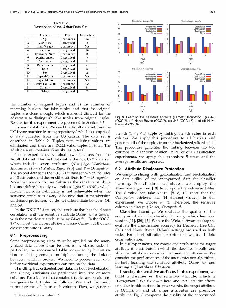
Learning the sensitive attribute. In this experiment, webuild a classifier on the sensitive attribute, which is“Occupation.” We fix c ¼ 2 here and evaluate the effectsof c later in this section. In other words, the target attributeis Occupation and all other attributes are predictorattributes. Fig. 3 compares the quality of the anonymized


1. http://archive.ics.uci.edu/ml/.

TABLE 2Description of the Adult Data Set

Fig. 3. Learning the sensitive attribute (Target: Occupation). (a) J48(OCC-7), (b) Naive Bayes (OCC-7), (c) J48 (OCC-15), and (d) NaiveBayes (OCC-15).

data (generated by the three techniques) with the quality of

the original data, when the target attribute is Occupation.

The experiments are performed on the two data sets OCC-7

(with seven attributes) and OCC-15 (with 15 attributes).

Fig. 3a (Fig. 3b) shows the classification accuracy of J48

(Naive Bayes) on the original data and the three anonymi-

zation techniques as a function of the ‘ value for the OCC-7

data set. Fig. 3c (Fig. 3d) shows the results for the OCC-15

data set.In all experiments, slicing outperforms both general-

ization and bucketization, that confirms that slicing pre-

serves attribute correlations between the sensitive attribute

and some QIs (recall that the sensitive column is {Gender,

Occupation}). Another observation is that bucketization

performs even slightly worse than generalization. That is

mostly due to our preprocessing step that randomly

associates the sensitive values to the QI values in each

bucket. This may introduce false associations while in

generalization, the associations are always correct although

the exact associations are hidden. A final observation is that

when ‘ increases, the performances of generalization and

bucketization deteriorate much faster than slicing. This also

confirms that slicing preserves better data utility in work-

loads involving the sensitive attribute.Learning a QI attribute. In this experiment, we build a

classifier on the QI attribute “Education.” We fix c ¼ 2 here

and evaluate the effects of c later in this section. In other

words, the target attribute is Education and all other

attributes including the sensitive attribute Occupation are

predictor attributes. Fig. 4 shows the experiment results.

Fig. 4a (Fig. 4b) shows the classification accuracy of J48

(Naive Bayes) on the original data and the three

anonymization techniques as a function of the ‘ value

for the OCC-7 data set. Fig. 4c (Fig. 4d) shows the results

for the data set OCC-15.

In all experiments, both bucketization and slicing performmuch better than generalization. This is because in bothbucketization and slicing, the QI attribute Education is in thesame column with many other QI attributes: in bucketiza-tion, all QI attributes are in the same column; in slicing, all QIattributes except Gender are in the same column. This factallows both approaches to perform well in workloadsinvolving the QI attributes. Note that the classificationaccuracies of bucketization and slicing are lower than that ofthe original data. This is because the sensitive attributeOccupation is closely correlated with the target attributeEducation (as mentioned earlier in Section 6, Education is thesecond closest attribute with Occupation in OCC-7). Bybreaking the link between Education and Occupation,classification accuracy on Education reduces for both buck-etization and slicing.

The effects of c. In this experiment, we evaluate the effectof c on classification accuracy. We fix ‘ ¼ 5 and vary thenumber of columns c in {2, 3, 5}. Fig. 5a shows the results onlearning the sensitive attribute and Fig. 5b shows the resultson learning a QI attribute. It can be seen that classificationaccuracy decreases only slightly when we increase c, becausethe most correlated attributes are still in the same column. Inall cases, slicing shows better accuracy than generalization.When the target attribute is the sensitive attribute, slicingeven performs better than bucketization.

Computational efficiency. We compare slicing withgeneralization and bucketization in terms of computationalefficiency. We fix ‘ ¼ 5 and vary the cardinality of the data(i.e., the number of records) and the dimensionality ofthe data (i.e., the number of attributes). Fig. 6a shows thecomputational time as a function of data cardinality wheredata dimensionality is fixed as 15 (i.e., we use (subsets) ofthe OCC-15 data set). Fig. 6b shows the computational timeas a function of data dimensionality where data cardinality


Fig. 4. Learning a QI attribute (Target: Education). (a) J48 (OCC-7),(b) Naive Bayes (OCC-7), (c) J48 (OCC-15), and (d) Naive Bayes(OCC-15).

Fig. 5. Varied c values. (a) Sensitive (OCC-15) and (b) QI (OCC-15).

Fig. 6. Computational efficiency. (a) Cardinality and (b) dimensionality.

is fixed as 45,222 (i.e., all records are used). The results showthat our slicing algorithm scales well with both datacardinality and data dimensionality.

6.3 Membership Disclosure Protection

In the second experiment, we evaluate the effectiveness ofslicing in membership disclosure protection.

We first show that bucketization is vulnerable tomembership disclosure. In both the OCC-7 data set andthe OCC-15 data set, each combination of QI values occursexactly once. This means that the adversary can determinethe membership information of any individual by checkingif the QI value appears in the bucketized data. If the QIvalue does not appear in the bucketized data, the individualis not in the original data. Otherwise, with high confidence,the individual is in the original data as no other individualhas the same QI value.

We then show that slicing does prevent membershipdisclosure. We perform the following experiment. First, wepartition attributes into c columns based on attributecorrelations. We set c 2 f2; 5g. In other words, we compare2-column-slicing with 5-column-slicing. For example, whenwe set c ¼ 5, we obtain five columns. In OCC-7, fAge,Marriage, Genderg is one column and each other attributeis in its own column. In OCC-15, the five columns are: fAge,Workclass, Education, Education-Num, Capital-Gain,Hours, Salaryg, fMarriage, Occupation, Family, Genderg,fRace, Countryg, fFinal-Weightg, and fCapital-Lossg.

Then, we randomly partition tuples into buckets of size p(the last bucket may have fewer than p tuples). As describedin Section 5, we collect statistics about the following twomeasures in our experiments: 1) the number of fake tuplesand 2) the number of matching buckets for original versusthe number of matching buckets for fake tuples.

The number of fake tuples. Fig. 7 shows the experimentalresults on the number of fake tuples, with respect to thebucket size p. Our results show that the number of fake tuplesis large enough to hide the original tuples. For example, forthe OCC-7 data set, even for a small bucket size of 100 andonly two columns, slicing introduces as many as 87,936 faketuples, which is nearly twice the number of original tuples(45,222). When we increase the bucket size, the number offake tuples becomes larger. This is consistent with ouranalysis that a bucket of size k can potentially matchkc � k fake tuples. In particular, when we increase thenumber of columns c, the number of fake tuples becomesexponentially larger. In almost all experiments, the numberof fake tuples is larger than the number of original tuples.The existence of such a large number of fake tuples provides

protection for membership information of the originaltuples.

The number of matching buckets. Fig. 8 shows thenumber of matching buckets for original tuples and faketuples.

We categorize the tuples (both original tuples and faketuples) into three categories: 1) �10: tuples that have at most10 matching buckets, 2) 10-20: tuples that have more than10 matching buckets but at most 20 matching buckets, and3) >20: tuples that have more than 20 matching buckets. Forexample, the “original-tuples(�10)” bar gives the number oforiginal tuples that have at most 10 matching buckets andthe “fake-tuples(>20)” bar gives the number of fake tuplesthat have more than 20 matching buckets. Because thenumber of fake tuples that have at most 10 matching bucketsis very large, we omit the “fake-tuples(�10)” bar from thefigures to make the figures more readable.

Our results show that, even when we do randomgrouping, many fake tuples have a large number ofmatching buckets. For example, for the OCC-7 data set,for a small p ¼ 100 and c ¼ 2, there are 5,325 fake tuplesthat have more than 20 matching buckets; the number is31,452 for original tuples. The numbers are even closer forlarger p and c values. This means that a larger bucket sizeand more columns provide better protection againstmembership disclosure.

Although many fake tuples have a large number ofmatching buckets, in general, original tuples have morematching buckets than fake tuples. As we can see from thefigures, a large fraction of original tuples have more than20 matching buckets while only a small fraction of faketuples have more than 20 tuples. This is mainly due tothe fact that we use random grouping in the experiments.The results of random grouping are that the number of faketuples is very large but most fake tuples have very fewmatching buckets. When we aim at protecting membershipinformation, we can design more effective grouping algo-rithms to ensure better protection against membership


Fig. 7. Number of fake tuples: (a) OCC-7 and (b) OCC-15.

Fig. 8. Number of tuples that have matching buckets. (a) 2-column(OCC-7), (b) 5-column (OCC-7), (c) 2-column (OCC-15), and(d) 5-column (OCC-15).

disclosure. The design of tuple grouping algorithms is left tofuture work.

7 THE NETFLIX PRIZE DATA SET

We emphasized the applicability of slicing on high-dimen-sional transactional databases. In this section, we experi-mentally evaluate the performance of slicing on the NetflixPrize data set2 that contains 100,480,507 ratings of17,770 movies contributed by 480,189 Netflix subscribers.Each rating has the following format: (userID, movieID,rating, date), where rating is an integer in f0; 1; 2; 3; 4; 5gwith 0 being the lowest rating and 5 being the highestrating.

To study the impact of the number of movies and thenumber of users on the performance, we choose a subset ofNetflix Prize data as the training data and vary the numberof movies and the number of users. Specifically, we choosethe first nMovies movies, and from all users that have ratedat least one of the nMovies movies, we randomly choose afraction fUsers of users. We evaluate the performance of ourapproach on this subset of Netflix Prize data.

Methodology. We use the standard SVD-based predic-tion method.3 As in Netflix Prize, prediction accuracy ismeasured as the rooted-mean-square-error (RMSE).

We compare slicing against the baseline method. Thebaseline method will simply predict any user’s rating on amovie as the average rating of that movie. Intuitively, thebaseline method considers the following data publishingalgorithm: the algorithm releases, for each movie, the averagerating of that movie from all users. The baseline method onlydepends on the global statistics of the data set and does notassume any knowledge about any particular user.

To use slicing, we measure the correlation of two moviesusing the cosine similarity measure

Simðm1;m2Þ ¼P

similarityðm1i;m2iÞjsuppðm1Þ [ suppðm2Þj

;

similarityðrating1; rating2Þ outputs 1 if both ratings aredefined and they are the same; it outputs 0 otherwise.suppðmÞ is the number of users who have rated movie m.Then, we can apply our slicing algorithm to anonymize thisdata set.

Finally, since the data set does not have a separation ofsensitive and nonsensitive movies, we randomly select�jnMoviesj as sensitive movies. Ratings on all other moviesare considered nonsensitive and are used as quasi-identify-ing attributes. Since the data set is sparse (a user has ratingsfor only a small fraction of movies), we “pad” the data set toreduce the sparsity. Specifically, if a user does not rate amovie, we replace this unknown rating by the averagerating of that movie.

Results. In our experiment, we fix nMovies ¼ 500 andfUsers ¼ 20 percent. We compare the RMSE errors from theoriginal data, the baseline method, and slicing. For slicing,

we chose c 2 f5; 10; 50g. We compare these five schemes interms of RMSE. Fig. 9 shows the RMSE of the five schemes.The results demonstrate that we can actually build accurateand privacy-preserving statistical learning models usingslicing. In Fig. 9a, we fix ‘ ¼ 3 and vary � 2 f0:05; 0:1; 0:3g.RMSE increases when � increases because it is more difficultto satisfy privacy for a larger � value. In Fig. 9b, we fix� ¼ 0:1 and vary ‘ 2 f2; 3; 4g. Similarly, RMSE increaseswhen ‘ increases.

The results also show the trade-off between the numberof columns c and prediction accuracy RMSE. Specifically,when we increase c, we lose attribute correlations withincolumns as each column contains a small set of attributes. Inthe meanwhile, we have smaller bucket sizes and poten-tially preserve better correlations across columns. Thistrade-off is demonstrated in our results; we get the bestresult when c ¼ 10. RMSE increases when c decreases to 5or increases to 50. Therefore, there is an optimal value for cwhere we can best utilize this trade-off.

8 RELATED WORK

Two popular anonymization techniques are generalizationand bucketization. Generalization [28], [30], [29] replaces avalue with a “less-specific but semantically consistent”value. Three types of encoding schemes have beenproposed for generalization: global recoding, regionalrecoding, and local recoding. Global recoding [18] has theproperty that multiple occurrences of the same value arealways replaced by the same generalized value. Regionalrecord [19] is also called multidimensional recoding (theMondrian algorithm) which partitions the domain spaceinto nonintersect regions and data points in the same regionare represented by the region they are in. Local recoding[36] does not have the above constraints and allowsdifferent occurrences of the same value to be generalizeddifferently. The main problems with generalization are: 1) itfails on high-dimensional data due to the curse ofdimensionality [1] and 2) it causes too much informationloss due to the uniform-distribution assumption [34].

Bucketization [34], [26], [17] first partitions tuples in thetable into buckets and then separates the quasi identifierswith the sensitive attribute by randomly permuting thesensitive attribute values in each bucket. The anonymizeddata consist of a set of buckets with permuted sensitiveattribute values. In particular, bucketization has been usedfor anonymizing high-dimensional data [12]. However,their approach assumes a clear separation between QIsand SAs. In addition, because the exact values of all QIs arereleased, membership information is disclosed. A detailed


2. The Netflix Prize data set is now available from the UCI MachineLearning Repository (http://archive.ics.uci.edu/ml/datasets/Netflix+Prize).

3. An implementation of the SVD method on the Netflix Prize data set isavailable here (http://www.timelydevelopment.com/demos/NetflixPrize.aspx).

Fig. 9. RMSE comparisions: (a) RMSE versus �and (b) RMSE versus ‘.

comparison of slicing with generalization and bucketizationis in Sections 2.2 and 2.3, respectively.

Slicing has some connections to marginal publication[16]; both of them release correlations among a subset ofattributes. Slicing is quite different from marginal publica-tion in a number of aspects. First, marginal publication canbe viewed as a special case of slicing which does not havehorizontal partitioning. Therefore, correlations amongattributes in different columns are lost in marginal publica-tion. By horizontal partitioning, attribute correlationsbetween different columns (at the bucket level) arepreserved. Marginal publication is similar to overlappingvertical partitioning, which is left as our future work (SeeSection 9). Second, the key idea of slicing is to preservecorrelations between highly correlated attributes and tobreak correlations between uncorrelated attributes thusachieving both better utility and better privacy. Third,existing data analysis (e.g., query answering) methods canbe easily used on the sliced data.

Recently, several approaches have been proposed toanonymize transactional databases. Terrovitis et al. [31]proposed the km-anonymity model which requires that, forany set of m or less items, the published database containsat least k transactions containing this set of items. Thismodel aims at protecting the database against an adversarywho has knowledge of at most m items in a specifictransaction. There are several problems with the km-anonymity model: 1) it cannot prevent an adversary fromlearning additional items because all k records may havesome other items in common; 2) the adversary may knowthe absence of an item and can potentially identify aparticular transaction; and 3) it is difficult to set anappropriate m value. He and Naughton [13] used k-anonymity as the privacy model and developed a localrecoding method for anonymizing transactional databases.The k-anonymity model also suffers from the first twoproblems above. Xu et al. [35] proposed an approach thatcombines k-anonymity and ‘-diversity but their approachconsiders a clear separation of the quasi identifiers and thesensitive attribute. On the contrary, slicing can be appliedwithout such a separation.

Existing privacy measures for membership disclosureprotection include differential privacy [6], [7], [9] and �-presence [27]. Differential privacy [6], [7], [9] has recentlyreceived much attention in data privacy. Most results ondifferential privacy are about answering statistical queries,rather than publishing microdata. A survey on these resultscan be found in [8]. On the other hand, �-presence [27]assumes that the published database is a sample of a largepublic database and the adversary has knowledge of thislarge database. The calculation of disclosure risk dependson the choice of this large database.

Finally, on attribute disclosure protection, a number ofprivacy models have been proposed, including ‘-diversity[25], ð�; kÞ-anonymity [33], and t-closeness [21]. A fewothers consider the adversary’s background knowledge[26], [4], [22], [24]. Wong et al. [32] considered adversarieswho have knowledge of the anonymization method.

9 DISCUSSIONS AND FUTURE WORK

This paper presents a new approach called slicing to privacy-preserving microdata publishing. Slicing overcomes the

limitations of generalization and bucketization and pre-serves better utility while protecting against privacy threats.We illustrate how to use slicing to prevent attributedisclosure and membership disclosure. Our experimentsshow that slicing preserves better data utility than general-ization and is more effective than bucketization in workloadsinvolving the sensitive attribute.

The general methodology proposed by this work is that:before anonymizing the data, one can analyze the datacharacteristics and use these characteristics in data anon-ymization. The rationale is that one can design better dataanonymization techniques when we know the data better.In [22], [24], we show that attribute correlations can be usedfor privacy attacks.

This work motivates several directions for future research.First, in this paper, we consider slicing where each attributeis in exactly one column. An extension is the notion ofoverlapping slicing, which duplicates an attribute in more thanone columns. This releases more attribute correlations. Forexample, in Table 1f, one could choose to include the Diseaseattribute also in the first column. That is, the two columns arefAge; Sex;Diseaseg and fZipcode;Diseaseg. This couldprovide better data utility, but the privacy implications needto be carefully studied and understood. It is interesting tostudy the trade-off between privacy and utility [23].

Second, we plan to study membership disclosureprotection in more details. Our experiments show thatrandom grouping is not very effective. We plan to designmore effective tuple grouping algorithms.

Third, slicing is a promising technique for handlinghigh-dimensional data. By partitioning attributes intocolumns, we protect privacy by breaking the associationof uncorrelated attributes and preserve data utility bypreserving the association between highly correlatedattributes. For example, slicing can be used for anonymiz-ing transaction databases, which has been studied recentlyin [31], [35], [13].

Finally, while a number of anonymization techniqueshave been designed, it remains an open problem on how touse the anonymized data. In our experiments, we randomlygenerate the associations between column values of abucket. This may lose data utility. Another direction is todesign data mining tasks using the anonymized data [14]computed by various anonymization techniques.

REFERENCES

[1] C. Aggarwal, “On k-Anonymity and the Curse of Dimension-ality,” Proc. Int’l Conf. Very Large Data Bases (VLDB), pp. 901-909,2005.

[2] A. Blum, C. Dwork, F. McSherry, and K. Nissim, “PracticalPrivacy: The SULQ Framework,” Proc. ACM Symp. Principles ofDatabase Systems (PODS), pp. 128-138, 2005.

[3] J. Brickell and V. Shmatikov, “The Cost of Privacy: Destruction ofData-Mining Utility in Anonymized Data Publishing,” Proc. ACMSIGKDD Int’l Conf. Knowledge Discovery and Data Mining (KDD),pp. 70-78, 2008.

[4] B.-C. Chen, K. LeFevre, and R. Ramakrishnan, “Privacy Skyline:Privacy with Multidimensional Adversarial Knowledge,” Proc.Int’l Conf. Very Large Data Bases (VLDB), pp. 770-781, 2007.

[5] H. Cramt’er, Mathematical Methods of Statistics. Princeton Univ.Press, 1948.

[6] I. Dinur and K. Nissim, “Revealing Information while PreservingPrivacy,” Proc. ACM Symp. Principles of Database Systems (PODS),pp. 202-210, 2003.


[7] C. Dwork, “Differential Privacy,” Proc. Int’l Colloquium Automata,Languages and Programming (ICALP), pp. 1-12, 2006.

[8] C. Dwork, “Differential Privacy: A Survey of Results,” Proc. FifthInt’l Conf. Theory and Applications of Models of Computation (TAMC),pp. 1-19, 2008.

[9] C. Dwork, F. McSherry, K. Nissim, and A. Smith, “CalibratingNoise to Sensitivity in Private Data Analysis,” Proc. Theory ofCryptography Conf. (TCC), pp. 265-284, 2006.

[10] J.H. Friedman, J.L. Bentley, and R.A. Finkel, “An Algorithm forFinding Best Matches in Logarithmic Expected Time,” ACM Trans.Math. Software, vol. 3, no. 3, pp. 209-226, 1977.

[11] B.C.M. Fung, K. Wang, and P.S. Yu, “Top-Down Specialization forInformation and Privacy Preservation,” Proc. Int’l Conf. Data Eng.(ICDE), pp. 205-216, 2005.

[12] G. Ghinita, Y. Tao, and P. Kalnis, “On the Anonymization ofSparse High-Dimensional Data,” Proc. IEEE 24th Int’l Conf. DataEng. (ICDE), pp. 715-724, 2008.

[13] Y. He and J. Naughton, “Anonymization of Set-Valued Data viaTop-Down, Local Generalization,” Proc. Int’l Conf. Very Large DataBases (VLDB), pp. 934-945, 2009.

[14] A. Inan, M. Kantarcioglu, and E. Bertino, “Using AnonymizedData for Classification,” Proc. IEEE 25th Int’l Conf. Data Eng.(ICDE), pp. 429-440, 2009.

[15] L. Kaufman and P. Rousueeuw, “Finding Groups in Data: AnIntroduction to Cluster Analysis,” John Wiley & Sons, 1990.

[16] D. Kifer and J. Gehrke, “Injecting Utility into Anonymized DataSets,” Proc. ACM SIGMOD Int’l Conf. Management of Data(SIGMOD), pp. 217-228, 2006.

[17] N. Koudas, D. Srivastava, T. Yu, and Q. Zhang, “Aggregate QueryAnswering on Anonymized Tables,” Proc. IEEE 23rd Int’l Conf.Data Eng. (ICDE), pp. 116-125, 2007.

[18] K. LeFevre, D. DeWitt, and R. Ramakrishnan, “Incognito: EfficientFull-Domain k-Anonymity,” Proc. ACM SIGMOD Int’l Conf.Management of Data (SIGMOD), pp. 49-60, 2005.

[19] K. LeFevre, D. DeWitt, and R. Ramakrishnan, “Mondrian Multi-dimensional k-Anonymity,” Proc. Int’l Conf. Data Eng. (ICDE),p. 25, 2006.

[20] K. LeFevre, D. DeWitt, and R. Ramakrishnan, “Workload-AwareAnonymization,” Proc. ACM SIGKDD Int’l Conf. KnowledgeDiscovery and Data Mining (KDD), pp. 277-286, 2006.

[21] N. Li, T. Li, and S. Venkatasubramanian, “t-Closeness: PrivacyBeyond k-Anonymity and ‘-Diversity,” Proc. IEEE 23rd Int’l Conf.Data Eng. (ICDE), pp. 106-115, 2007.

[22] T. Li and N. Li, “Injector: Mining Background Knowledge for DataAnonymization,” Proc. IEEE 24th Int’l Conf. Data Eng. (ICDE),pp. 446-455, 2008.

[23] T. Li and N. Li, “On the Tradeoff between Privacy and Utility inData Publishing,” Proc. ACM SIGKDD Int’l Conf. KnowledgeDiscovery and Data Mining (KDD), pp. 517-526, 2009.

[24] T. Li, N. Li, and J. Zhang, “Modeling and Integrating BackgroundKnowledge in Data Anonymization,” Proc. IEEE 25th Int’l Conf.Data Eng. (ICDE), pp. 6-17, 2009.

[25] A. Machanavajjhala, J. Gehrke, D. Kifer, and M. Venkitasubrama-niam, “‘-Diversity: Privacy Beyond k-Anonymity,” Proc. Int’l Conf.Data Eng. (ICDE), p. 24, 2006.

[26] D.J. Martin, D. Kifer, A. Machanavajjhala, J. Gehrke, and J.Y.Halpern, “Worst-Case Background Knowledge for Privacy-Preserving Data Publishing,” Proc. IEEE 23rd Int’l Conf. DataEng. (ICDE), pp. 126-135, 2007.

[27] M.E. Nergiz, M. Atzori, and C. Clifton, “Hiding the Presence ofIndividuals from Shared Databases,” Proc. ACM SIGMOD Int’lConf. Management of Data (SIGMOD), pp. 665-676, 2007.

[28] P. Samarati, “Protecting Respondent’s Privacy in MicrodataRelease,” IEEE Trans. Knowledge and Data Eng., vol. 13, no. 6,pp. 1010-1027, Nov./Dec. 2001.

[29] L. Sweeney, “Achieving k-Anonymity Privacy Protection UsingGeneralization and Suppression,” Int’l J. Uncertainty Fuzziness andKnowledge-Based Systems, vol. 10, no. 6, pp. 571-588, 2002.

[30] L. Sweeney, “k-Anonymity: A Model for Protecting Privacy,” Int’lJ. Uncertainty Fuzziness and Knowledge-Based Systems, vol. 10, no. 5,pp. 557-570, 2002.

[31] M. Terrovitis, N. Mamoulis, and P. Kalnis, “Privacy-PreservingAnonymization of Set-Valued Data,” Proc. Int’l Conf. Very LargeData Bases (VLDB), pp. 115-125, 2008.

[32] R.C.-W. Wong, A.W.-C. Fu, K. Wang, and J. Pei, “MinimalityAttack in Privacy Preserving Data Publishing,” Proc. Int’l Conf.Very Large Data Bases (VLDB), pp. 543-554, 2007.

[33] R.C.-W. Wong, J. Li, A.W.-C. Fu, and K. Wang, “(�, k)-Anonymity:An Enhanced k-Anonymity Model for Privacy Preserving DataPublishing,” Proc. ACM SIGKDD Int’l Conf. Knowledge Discoveryand Data Mining (KDD), pp. 754-759, 2006.

[34] X. Xiao and Y. Tao, “Anatomy: Simple and Effective PrivacyPreservation,” Proc. Int’l Conf. Very Large Data Bases (VLDB),pp. 139-150, 2006.

[35] Y. Xu, K. Wang, A.W.-C. Fu, and P.S. Yu, “AnonymizingTransaction Databases for Publication,” Proc. ACM SIGKDD Int’lConf. Knowledge Discovery and Data Mining (KDD), pp. 767-775,2008.

[36] J. Xu, W. Wang, J. Pei, X. Wang, B. Shi, and A.W.-C. Fu, “Utility-Based Anonymization Using Local Recoding,” Proc. 12th ACMSIGKDD Int’l Conf. Knowledge Discovery and Data Mining (KDD),pp. 785-790, 2006.

Tiancheng Li received the BE degree incomputer science from Zhejiang University in2005. He is currently working toward thePhD degree in the Department of ComputerScience and the Center for Education andResearch in Information Assurance and Se-curity (CERIAS) at Purdue University. Hisresearch interests are in the area of data-bases, data mining, information security andprivacy, and applied cryptography, with a focus

on privacy preserving data publishing and sharing.

Ninghui Li received the BE degree in computerscience from the University of Science andTechnology of China in 1993, and the MSc andPhD degrees in computer science from NewYork University, in 1998 and 2000. He iscurrently an assistant professor in ComputerScience at Purdue University. Prior to joiningPurdue University in 2003, he was a researchassociate at Stanford University ComputerScience Department. His research interests are

in security and privacy in information systems, with a focus on accesscontrol. He has worked on projects on trust management, automatedtrust negotiation, role-based access control, online privacy protection,privacy-preserving data publishing, and operating system accesscontrol. He has published more than 50 technical papers in refereedjournals and conference proceedings and has served on the ProgramCommittees of more than three dozen international conferences andworkshops. He is a member of the ACM and the USENIX Associationand a senior member of the IEEE.

Jian Zhang received the BS degree from OceanUniversity of China, the MS degree from ChineseAcademy of Sciences, and the PhD degree fromCarnegie Mellon University. He is an assistantprofessor in the Department of Statistics atPurdue University. His research interests includestatistical machine learning, computational sta-tistics, and information retrieval. He is a memberof the IEEE and the IEEE Computer Society.

Ian Molloy is working toward the PhD degree inthe Center for Education and Research inInformation Assurance and Security at PurdueUniversity. His research interests include accesscontrol, applied cryptography, and privacy. Inparticular, he is interested in the application ofdata mining and machine learning to problems insecurity and information assurance. His primaryfocus is on the application of data mining to

problems in role engineering and role-based access control, and newmodels for access control and secure information sharing.

. For more information on this or any other computing topic,please visit our Digital Library at www.computer.org/publications/dlib.


155141903 Slicing a New Approach for Privacy Preserving Data Publishing

Documents

Transcript of 155141903 Slicing a New Approach for Privacy Preserving Data Publishing