15.3 The F Test for a Randomized Block Experiment The F Test for a Randomized Block Experiment ......

........................................................................................................................................

15.3 The F Test for a Randomized Block Experiment We saw in Chapter 11 that when two treatments are to be compared, a paired experimentis often more effective than one involving two independent samples. This is becausepairing can considerably reduce the extraneous variation in subjects or experimentalunits. A similar result can be achieved when more than two treatments are to be com-pared. Suppose that four different pesticides (the treatments) are being considered forapplication to a particular crop. There are 20 plots of land available for planting. If 5of these plots are randomly selected to receive Pesticide 1, 5 of the remaining 15 ran-domly selected for Pesticide 2, and so on, the result is a completely randomized exper-iment, and the data should be analyzed using a single-factor ANOVA. The disadvan-tage of this experiment is that if there are any substantial differences in characteristicsof the plots that could affect yield, a separate assessment of any differences betweentreatments will not be possible (because any difference in means could be attributedto either treatments or characteristics of the plot, plot effects are confounded withtreatment effects).

Here is an alternative experiment. Consider separating the 20 plots into 5 groups,each consisting of 4 plots. Within each group, the plots are as much alike as possiblewith respect to characteristics affecting yield. Then, within each group one plot is ran-domly selected for Pesticide 1, a second plot is randomly chosen to receive Pesticide 2,and so on. The homogeneous groups are called blocks, and the random allocation oftreatments within each block as described results in a randomized block experiment.

. . . . . . . . . . . ........ .. .. .. .. .. .. .. .. .. .. .. .. . . . . . . . . . . .....................................................................................

Example 15.8 Cost of Air-Conditioning: Type of System Blocked byHouse Type

� High energy costs have made consumers and home builders increasingly aware ofwhether household appliances are energy efficient. A large developer carried out astudy to compare electricity usage for four different residential air-conditioning sys-tems being considered for tract homes. Each system was installed in five homes, andthe resulting electricity usage (in kilowatt-hours) was monitored for a 1-month period.Because the developer realized that many characteristics of a home could affect usage(e.g., floor space, type of insulation, directional orientation, and type of roof and exte-rior), care was taken to ensure that extraneous variation in such characteristics did not

D E F I N I T I O N

Suppose that experimental units (individuals or objects to which the treat-ments are applied) are first separated into groups consisting of k units insuch a way that the units within each group are as similar as possible.Within any particular group, the treatments are then randomly allocated so that each unit in a group receives a different treatment. The groups arecalled blocks, and the experimental design is referred to as a randomizedblock design.

15.3 � The F Test for a Randomized Block Experiment 15-1

� Data set available online

15-W4008(online) 2/28/07 6:39 AM 5-1

The mi notation used previously is no longer adequate for stating hypotheses, be-cause an observation’s mean value may depend on both the treatment applied and theblock.

� The F Test . .. .. .. .. .. .. .. .. . . . . . . . . . . ..................................................................................

The key to analyzing data from a randomized block experiment is to represent SSTo,which measures total variation, as a sum of three pieces: SSTr and SSE (as was thecase in single-factor ANOVA), and a new contribution to variation, the block sum ofsquares SSBl. SSBl incorporates any variation resulting from differences between theblocks; these differences can be substantial if, before creating the blocks, there wasgreat heterogeneity in experimental units. Once the four sums of squares have been

15-2 C h a p t e r 15 � Analysis of Variance

influence the conclusions. Homes selected for the experiment were grouped into fiveblocks consisting of four homes each in such a way that the four homes within anygiven block were as similar as possible. The resulting data are displayed in Table 15.5,in which rows correspond to the different treatments (air-conditioning systems) andcolumns correspond to the different blocks. Later in this section we will analyze thesedata to see whether electricity usage depends on which system is used.

Table 15.5 Data from the Randomized Block Experiment of Example 15.8

BlockTreatment

Treatment 1 2 3 4 5 Average

1 116 118 97 101 115 109.402 171 131 105 107 129 128.603 138 131 115 93 110 117.404 144 141 115 93 99 118.40

Block average 142.25 130.25 108.00 98.50 113.25 Grand mean 118.45

�

The hypotheses of interest and assumptions underlying the analysis of a random-ized block design are similar to those for a completely randomized design.

Assumpt ions and Hypotheses

The single observation made on any particular treatment in a given block is assumed to be se-lected from a normal distribution with variance s2. Although the mean of the distribution maydepend separately on the treatment applied and on the block, the variance s2 is assumed to bethe same for each block–treatment combination.

The hypotheses of interest are as follows:

H0: The mean value does not depend on which treatment is applied.Ha: The mean value does depend on which treatment is applied.

15-W4008(online) 2/28/07 6:39 AM Page 15-2

Alternative formulas for the sums of squares appropriate for efficient hand com-putation appear in the online appendix to this chapter.

Calculations for this F test are usually summarized in an ANOVA table. The tableis similar to the one for a single-factor ANOVA except that blocks are an extra sourceof variation, so four rows are included rather than just three, consistent with the addedsource of variation.

Table 15.6 shows a mean square for blocks and the mean squares for treatmentsand error. Sometimes the F ratio MSBl/MSE is also computed. A large value of thisratio suggests that blocking was effective in filtering out extraneous variation.


computed, the test statistic is an F ratio, MSTr/MSE, but the number of error degreesof freedom is no longer N � k as it was in single-factor ANOVA.

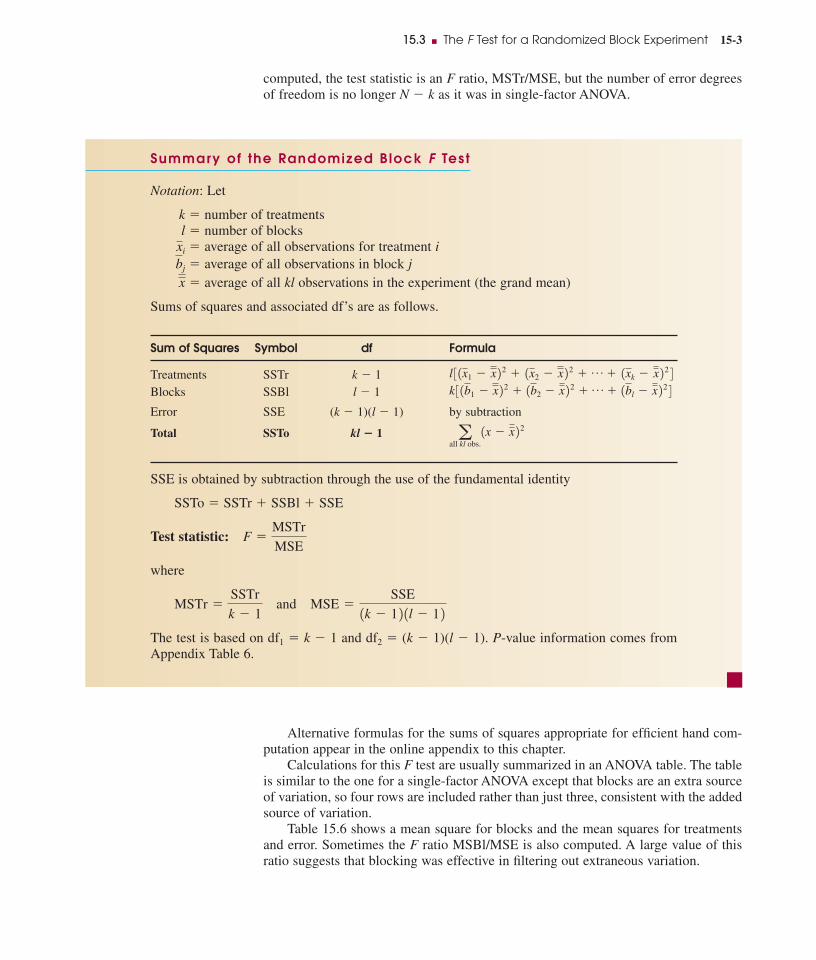
Summary of the Randomized Block F Test

Notation: Let

k � number of treatmentsl � number of blocks

� average of all observations for treatment i� average of all observations in block j� average of all kl observations in the experiment (the grand mean)

Sums of squares and associated df’s are as follows.

Sum of Squares Symbol df Formula

Treatments SSTr k � 1 Blocks SSBl l � 1

Error SSE (k � 1)(l � 1) by subtraction

Total SSTo kl � 1

SSE is obtained by subtraction through the use of the fundamental identity

SSTo � SSTr � SSBl � SSE

Test statistic:

where

The test is based on df1 � k � 1 and df2 � (k � 1)(l � 1). P-value information comes fromAppendix Table 6.

MSTr �SSTr

k � 1 and MSE �

SSE

1k � 1 2 1l � 1 2

F �MSTr

MSE

aall kl obs.

1x � x 2 2k 3 1b1 � x 2 2 � 1b2 � x 2 2 � p � 1bl � x 2 2 4l 3 1x1 � x 2 2 � 1x2 � x 2 2 � p � 1xk � x 2 2 4

xbj

xi

15-W4008(online) 2/28/07 6:39 AM Page 15-3

Table 15.6 ANOVA Table for a Randomized Block Experiment

Source of Sum of Mean Variation df Squares Square F

Treatments k � 1 SSTr

Blocks l � 1 SSBl

Error (k � 1)(l � 1) SSE

Total kl � 1 SSTo

..................... .. .. .. .. .. .. .. .. .. .. .. .. . . . . . . . . . . ...................................................................................

Example 15.9 Electricity Cost of Air-Conditioning Revisited

Reconsider the electricity usage data given in Example 15.8.

H0: The mean electricity usage does not depend on which air-conditioning system is used.

Ha: The mean electricity usage does depend on which system is used.

Test Statistic:

From Example 15.8,

(these are the four row averages), and

(these are the five column averages). Using the individual observations given previously,

The other sums of squares are

The remaining calculations are displayed in the accompanying ANOVA table.

� 1705.10 � 7594.95 � 930.15 � 4959.70

SSE � SSTo � SSTr � SSBl

� 4959.70 � 4 3 1142.25 � 118.45 2 2 � 1130.25 � 118.45 2 2 � p � 1113.25 � 118.45 2 2 4 SSBl � k 3 1b1 � x 2 2 � 1b2 � x 2 2 � p � 1bl � x 2 2 4 � 930.15 � 1117.4 � 118.45 2 2 � 1118.4 � 118.45 2 2 4 � 5 3 1109.4 � 118.45 2 2 � 1128.6 � 118.45 2 2 SSTr � l 3 1x1 � x 2 2 � 1x2 � x 2 2 � p � 1xk � x 2 2 4

� 7594.95 � 1116 � 118.45 2 2 � 1118 � 118.45 2 2 � p � 199 � 118.45 2 2

SSTo � aall kl obs.

1x � x 2 2

b1 � 142.25 b2 � 130.25 b3 � 108.00 b4 � 98.50 b5 � 113.25

x1 � 109.40 x2 � 128.60 x3 � 117.40 x4 � 118.40 x � 118.45

F �MSTr

MSE

MSE �SSE

1k � 1 2 1l � 1 2

MSBl �SSBl

l � 1

F �MSTr

MSE MSTr �

SSTr

k � 1


15-W4008(online) 2/28/07 6:39 AM Page 15-4


Treatments 3 930.15 310.05

Blocks 4 4959.70 1239.93Error 12 1705.10 142.09Total 19 7594.95

In Appendix Table 6 with df1 � 3 and df2 � 12, the value 2.61 corresponds to aP-value of .10. Since 2.18 � 2.61, P-value � .10 and H0 cannot be rejected. Meanelectricity usage does not seem to depend on which of the four air-conditioning sys-tems is used.

�

In many studies, all k treatments can be applied to the same experimental unit, sothere is no need to group different experimental units to form blocks. For example, anexperiment to compare the effects of four different gasoline additives on automobileengine efficiency could be carried out by selecting just 5 engines and using all fourtreatments on each one rather than using 20 engines and blocking them. Each en-gine by itself then constitutes a block. As another example, a manufacturing companymight wish to compare outputs for three different packaging machines. Because out-put could be affected by which operator is using the machine, a design that controlsfor the effects of operator variation is desirable. One possibility is to use 15 operatorsgrouped into homogeneous blocks of 5 operators each, but such homogeneity withineach block may be difficult to achieve. An alternative approach is to use only five op-erators and to have each one operate all three machines in a randomly chosen order.There are then three observations in each block, all three with the same operator.

................... .. .. .. .. .. .. .. .. .. .. .. .. . . . . . . . . . . .....................................................................................

Example 15.10 Comparing Four Stool Designs

� In the article “The Effects of a Pneumatic Stool and a One-Legged Stool on LowerLimb Joint Load and Muscular Activity During Sitting and Rising” (Ergonomics[1993]: 519–535), the accompanying data were given on the effort (measured on theBorg Scale) required by a subject to rise from a sitting position for each of four differ-ent stools. Because it was suspected that different people could exhibit large differ-ences in effort, even for the same type of stool, a sample of nine people was selectedand each person was tested on all four stools, with the following results:

Subject

1 2 3 4 5 6 7 8 9

Stool A 12 10 7 7 8 9 8 7 9Stool B 15 14 14 11 11 11 12 11 13Stool C 12 13 13 10 08 11 12 8 10Stool D 10 12 9 9 7 10 11 7 8

310.05

142.09� 2.18


Step-by-step technology instructions available online � Data set available online

15-W4008(online) 2/28/07 6:39 AM Page 15-5


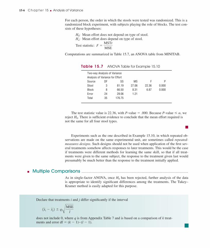
For each person, the order in which the stools were tested was randomized. This is arandomized block experiment, with subjects playing the role of blocks. The test con-sists of these hypotheses:

H0: Mean effort does not depend on type of stool.Ha: Mean effort does depend on type of stool.

Test statistic:

Computations are summarized in Table 15.7, an ANOVA table from MINITAB.

Table 15.7 ANOVA Table for Example 15.10

Two-way Analysis of VarianceAnalysis of Variance for EffortSource DF SS MS F PStool 3 81.19 27.06 22.36 0.000Block 8 66.50 8.31 6.87 0.000Error 24 29.06 1.21Total 35 176.75

The test statistic value is 22.36, with P-value � .000. Because P-value � a, wereject H0. There is sufficient evidence to conclude that the mean effort required isnot the same for all four stool types.

�

Experiments such as the one described in Example 15.10, in which repeated ob-servations are made on the same experimental unit, are sometimes called repeated-measures designs. Such designs should not be used when application of the first sev-eral treatments somehow affects responses to later treatments. This would be the caseif treatments were different methods for learning the same skill, so that if all treat-ments were given to the same subject, the response to the treatment given last wouldpresumably be much better than the response to the treatment initially applied.

� Multiple Comparisons . . . . ...................................................................................

As in single-factor ANOVA, once H0 has been rejected, further analysis of the datais appropriate to identify significant differences among the treatments. The Tukey–Kramer method is easily adapted for this purpose.

F �MSTr

MSE

Declare that treatments i and j differ significantly if the interval

does not include 0, where q is from Appendix Table 7 and is based on a comparison of k treat-ments and error df � (k � 1) (l � 1).#

1xi � xj 2 � q BMSE

l

15-W4008(online) 2/28/07 6:39 AM Page 15-6

� E x e r c i s e s 15.35–15.43

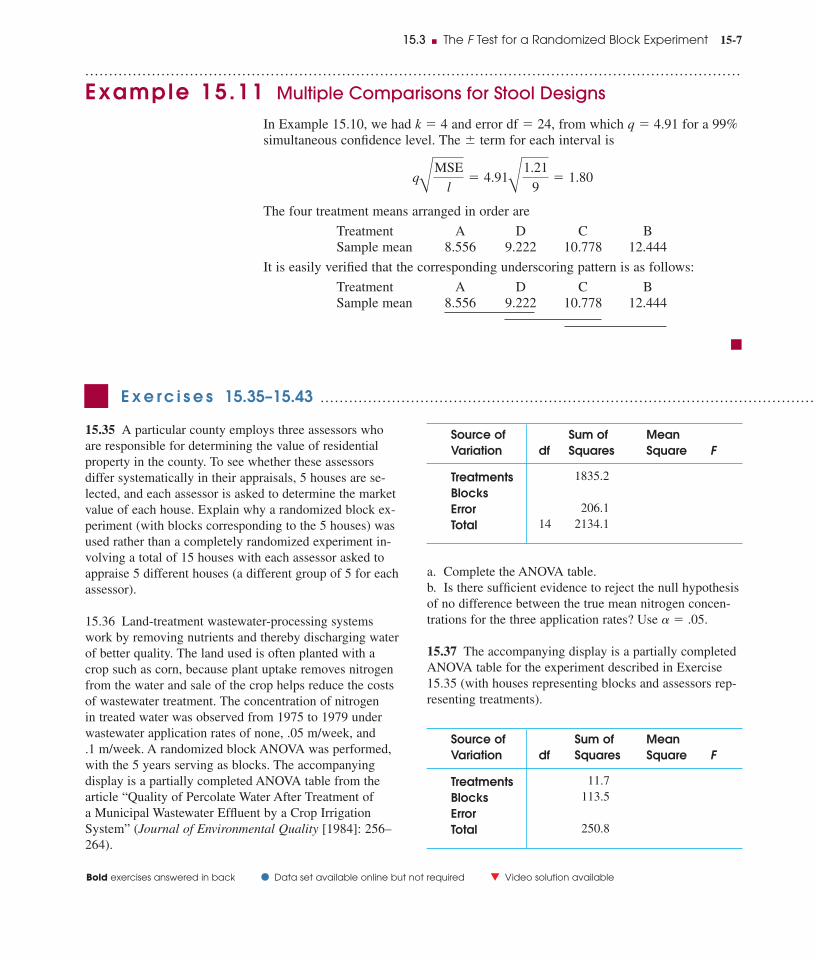
15.35 A particular county employs three assessors whoare responsible for determining the value of residentialproperty in the county. To see whether these assessorsdiffer systematically in their appraisals, 5 houses are se-lected, and each assessor is asked to determine the marketvalue of each house. Explain why a randomized block ex-periment (with blocks corresponding to the 5 houses) wasused rather than a completely randomized experiment in-volving a total of 15 houses with each assessor asked toappraise 5 different houses (a different group of 5 for eachassessor).

15.36 Land-treatment wastewater-processing systemswork by removing nutrients and thereby discharging waterof better quality. The land used is often planted with acrop such as corn, because plant uptake removes nitrogenfrom the water and sale of the crop helps reduce the costsof wastewater treatment. The concentration of nitrogen in treated water was observed from 1975 to 1979 underwastewater application rates of none, .05 m/week, and .1 m/week. A randomized block ANOVA was performed,with the 5 years serving as blocks. The accompanying display is a partially completed ANOVA table from the article “Quality of Percolate Water After Treatment of a Municipal Wastewater Effluent by a Crop Irrigation System” (Journal of Environmental Quality [1984]: 256–264).


Treatments 1835.2BlocksError 206.1Total 14 2134.1

a. Complete the ANOVA table.b. Is there sufficient evidence to reject the null hypothesisof no difference between the true mean nitrogen concen-trations for the three application rates? Use a � .05.

15.37 The accompanying display is a partially completedANOVA table for the experiment described in Exercise15.35 (with houses representing blocks and assessors rep-resenting treatments).


Treatments 11.7Blocks 113.5ErrorTotal 250.8


................... .. .. .. .. .. .. .. .. .. .. .. .. . . . . . . . . . . .....................................................................................

Example 15.11 Multiple Comparisons for Stool Designs

In Example 15.10, we had k � 4 and error df � 24, from which q � 4.91 for a 99%simultaneous confidence level. The � term for each interval is

The four treatment means arranged in order are

Treatment A D C BSample mean 8.556 9.222 10.778 12.444

It is easily verified that the corresponding underscoring pattern is as follows:

Treatment A D C BSample mean 8.556 9.222 10.778 12.444

�

qBMSE

l� 4.91B1.21

9� 1.80

................................................................ ............ ................................

Bold exercises answered in back � Data set available online but not required � Video solution available

15-W4008(online) 2/28/07 6:39 AM Page 15-7

a. Fill in the missing entries in the ANOVA table.b. Use the ANOVA F statistic and a .05 level of signifi-cance to test the null hypothesis of no difference betweenassessors.

15.38 The article “Rate of Stuttering Adaptation UnderTwo Electro-Shock Conditions” (Behavior Research Ther-apy [1967]: 49–54) gave adaptation scores for three differ-ent treatments: no shock (Treatment 1), shock followingeach stuttered word (Treatment 2), and shock during eachmoment of stuttering (Treatment 3). These treatmentswere used on each of 18 stutterers. The 18 subjects wereviewed as blocks, and the data were analyzed using a ran-domized block ANOVA. Summary quantities are SSTr �28.78, SSBl � 2977.67, and SSE � 469.55. Construct the ANOVA table, and test at significance level .05 to seewhether true average adaptation score depends on thetreatment given.

15.39 � The accompanying table shows average height of cotton plants during 1978–1980 under three differenteffluent application rates (350, 440, and 515 mm) (“DripIrrigation of Cotton with Treated Municipal Effluents:Yield Response,” Journal of Environmental Quality [1984]:231–238).

Application Rate

Year 350 440 515

1978 166 176 1771979 109 126 1361980 140 155 156

a. These data were analyzed using a randomized blockANOVA, with years serving as blocks. Explain why thiswould be better for comparing treatments than a com-pletely randomized ANOVA.b. With Treatments 1, 2, and 3 denoting the applicationrates 350, 440, and 515, respectively, summary quanti-ties are

Construct an ANOVA table. Using a � .05, determinewhether the true mean height differs for the three effluentrates.

b3 � 150.33b2 � 123.67b1 � 173.00x3 � 156.33x2 � 152.33x1 � 138.33

x � 149.00g 1x � x 2 2 � 4266.0

c. Identify significant differences among the rates. (Hint:q � 5.04)

15.40 � The article “Responsiveness of Food Sales toShelf Space Changes in Supermarkets” (Journal of Mar-keting Research [1964]: 63–67) described an experimentto assess the effect of allotted shelf space on product sales.Two of the products studied were baking soda (a stapleproduct) and Tang (considered to be an impulse product).Six stores (blocks) were used in the experiment, and sixdifferent shelf-space allotments were tried for 1 weekeach. Space allotments of 2, 4, 6, 8, 10, and 12 ft wereused for baking soda, and 6, 9, 12, 15, 18, and 21 ft wereused for Tang. The author speculated that sales of staplegoods would not be sensitive to changes in shelf space,whereas sales of impulse products would be affected bychanges in shelf space. Data on number of boxes of bak-ing soda and on number of containers of Tang sold duringa 1-week period are given in the accompanying tables.Construct ANOVA tables and test the appropriate hypothe-ses. Use a significance level of .05. Was the author correctin his speculation that sales of the staple product wouldnot be affected by shelf space allocation, whereas sales ofthe impulse product would be affected? Explain.

Baking Soda Shelf Space

Store 2 4 6 8 10 12

1 36 42 36 40 30 222 74 61 65 67 83 843 40 58 42 73 69 634 43 65 65 41 43 475 27 33 35 17 40 266 23 31 36 38 42 37

Tang Shelf Space

Store 6 9 12 15 18 21

1 30 35 25 25 38 312 47 59 43 62 65 483 47 55 48 54 36 544 29 19 41 27 33 395 17 11 25 23 24 266 22 9 19 18 25 22

15.41 � The article “Measuring Treatment Effects ThroughComparisons Along Plot Boundaries” (Forest Science



15-W4008(online) 2/28/07 6:39 AM Page 15-8

........................................................................................................................................

15.4 Two-Factor ANOVAAn investigator is often interested in assessing the effects of two different factors on aresponse variable. Consider the following examples.

1. A physical education researcher wishes to know how body density of football play-ers varies with position played (a categorical factor with categories defensive back,offensive back, defensive lineman, and offensive lineman) and level of play (a sec-ond categorical factor with categories professional, college Division I, college Di-vision II, and college Division III).

2. An agricultural scientist is interested in seeing how yield of tomatoes is affected bychoice of variety planted (a categorical factor, with each category corresponding toa different variety) and planting density (a quantitative factor, with a level corre-sponding to each planting density being considered).

3. An applied chemist might wish to investigate how shear strength of a particular ad-hesive varies with application temperature (a quantitative factor with levels 250F,260F, and 270F) and application pressure (a quantitative factor with levels 110,120, 130, and 140 lb/in.2).

15.4 � Two-Factor ANOVA 15-9

[1980]: 704–709) reported the results of a randomizedblock experiment. Five different sources of pine seed wereused in each of four blocks. The accompanying table givesdata on plant height (m). Do the data provide sufficient evi-dence to conclude that the true mean height is not the samefor all five seed sources? Use a .05 level of significance.

Block

Source I II III IV

1 7.1 5.8 7.2 6.92 6.2 5.3 7.7 4.73 7.9 5.4 8.6 6.24 9.0 5.9 5.7 7.35 7.0 6.3 4.4 6.1

15.42 � The article cited in Exercise 15.41 also gave theaccompanying data on survival rate for five different seedsources.

Block

Source I II III IV

1 62.5 87.5 50.0 70.32 50.0 50.0 54.7 59.43 93.8 92.2 87.5 87.54 96.9 76.6 70.3 65.65 56.3 50.0 45.3 56.3

a. Construct an ANOVA table and test the null hypothesisof no difference in true mean survival rates for the fiveseed sources. Use a � .05.b. Use multiple comparisons to identify significant differ-ences among the seed sources. (Hint: q � 5.04)

15.43 In a comparison of the energy efficiency of threetypes of ovens (conventional, biradiant, and convection),the energy used in cooking was measured for eight differ-ent foods (one-layer cake, two-layer cake, biscuits, bread,frozen pie, baked potatoes, lasagna, and meat loaf). Sincea comparison between the three types of ovens is desired,a randomized block ANOVA (with the eight foods servingas blocks) will be used. Suppose calculations result in thequantities SSTo � 4.57, SSTr � 3.97, and SSBl � .2503.(A similar study is described in the article “OptimizingOven Radiant Energy Use,” Home Economics ResearchJournal [1980]: 242–251.) Construct an ANOVA table andtest the null hypothesis of no difference in mean energyuse for the three types of ovens. Use a .01 significancelevel.


15-W4008(online) 2/28/07 6:39 AM Page 15-9

Suppose that an experiment is carried out, resulting in a data set that containssome number of observations for each of the kl treatments. In general, there could bemore observations for some treatments than for others, and there may even be a fewtreatments for which no observations are available. An experimenter may set out tomake the same number of observations on each treatment, but, occasionally, forces be-yond the experimenter’s control—the death of an experimental subject, malfunction-ing equipment, and so on—result in different sample sizes for some treatments. Suchimbalances in sample sizes makes analysis of the data rather difficult. We will restrictour discussion to consideration of data sets containing the same number of observa-tions for each treatment, and we will let m denote this number.


Let’s label the two factors under study Factor A and Factor B. Even when a fac-tor is categorical, it simplifies terminology to refer to the categories as levels. Thus, inthe first example, the categorical factor position played has four levels. The number oflevels of Factor A is denoted by k, and l denotes the number of levels of Factor B, asshown in Table 15.8. This rectangular table contains a row corresponding to each levelof Factor A and a column corresponding to each level of Factor B. Each cell in thetable corresponds to a particular level of Factor A in combination with a particularlevel of Factor B. Because there are l cells in each row and k rows, there are kl cells inthe table. The kl different combinations of Factor A and Factor B levels are often re-ferred to as treatments. For example, if there are three tomato varieties and four dif-ferent planting densities under consideration, the number of treatments is 12.

Factor B levels1 2 l

1

2

k

��

� � � �

Fac

tor A

leve

ls

Table 15.8 A Table of FactorCombinations for aTwo-Way ANOVAExperiment

Notat ion

k � number of levels of Factor A l � number of levels of Factor B

kl � number of treatments (each one a combination of a Factor A level and a Factor B level)m � number of observations on each treatment

15-W4008(online) 2/28/07 6:39 AM Page 15-10

................... .. .. .. .. .. .. .. .. .. .. .. .. . . . . . . . . . . .....................................................................................

Example 15.12 Tomato Yield and Planting Density

� An experiment was carried out to assess the effects of tomato variety (Factor A,with k � 3 levels) and planting density (Factor B, with l � 4 levels of 10,000, 20,000,30,000, and 40,000 plants per hectare) on yield. Each of the kl � 12 treatments wasused on m � 3 plots, resulting in the data set consisting of klm � 36 observationsshown in Table 15.9 (adapted from “Effects of Plant Density on Tomato Yields inWestern Nigeria,” Experimental Agriculture [1976]: 43–47).

Table 15.9 Data from the Two-Factor Experiment of Example 15.12

VarietyDensity (Factor B)

(Factor A) 1 2 3 4

1 7.9, 9.2, 10.5 11.2, 12.8, 13.3 12.1, 12.6, 14.0 9.1, 10.8, 12.502 8.1, 8.6, 10.1 11.5, 12.7, 13.7 13.7, 14.4, 15.4 11.3, 12.5, 14.53 15.3, 16.1, 17.5 16.6, 18.5, 19.2 18.0, 20.8, 21.0 17.2, 18.4, 18.9

Sample average yields for each treatment, each level of Factor A, and each levelof Factor B are important summary quantities. These can be displayed in a rectangu-lar table (see Table 15.10). A plot of these sample averages is also quite informative.First, construct horizontal and vertical axes, and scale the vertical axis in units of theresponse variable (yield). Then mark a point on the horizontal axis for each level ofone of the factors (either Factor A or Factor B can be chosen). Now above each suchmark, plot a point for the sample average response for each level of the other factor.Finally, connect all points corresponding to the same level of the other factor usingstraight line segments.

Table 15.10 Sample Means for the 12 Treatments of Example 15.12

Sample AverageFactor A

Factor B (Planting Density)Yield for Each

(Variety) 1 2 3 4 Level of Factor A

1 9.20 12.43 12.90 10.80 11.332 8.93 12.63 14.50 12.77 12.213 16.30 18.10 19.93 18.17 18.13

Sample AverageYield for EachLevel of Factor B 11.48 14.39 15.78 13.91 Grand mean � 13.89

Figure 15.10 displays two plots: one in which Factor A levels mark the horizon-tal axis and one in which Factor B levels mark the horizontal axis; usually only oneof the two plots is constructed.


� Data set available online

15-W4008(online) 2/28/07 6:39 AM Page 15-11

�

� Interaction .. .. .. .. .. .. .. . . . . . . . . . . ............................................................ .......................

An important aspect of two-factor studies involves assessing how simultaneouschanges in the levels of both factors affect the response. As a simple example, supposethat an automobile manufacturer is studying engine efficiency (measured in miles per gallon) for two different engine sizes (Factor A, with k � 2 levels) in combinationwith two different carburetor designs (Factor B, with l � 2 levels). Consider the twopossible sets of true average responses displayed in Figure 15.11. In Figure 15.11(a),when Factor A changes from Level 1 to Level 2 and Factor B remains at Level 1 (thechange within the first column), the true average response increases by 2. Similarly,

when Factor B changes from Level 1 to Level 2 and Factor Ais fixed at Level 1 (the change within the first row), the true average response increases by 3. And when the levels ofboth factors are changed from 1 to 2, the true average re-sponse increases by 5, which is the sum of the two “one-at-a-time” increases. This is because the change in true averageresponse when the level of either factor changes from 1 to 2is the same for each level of the other factor: The changewithin either row is 3, and the change within either column is 2. In this case, changes in the levels of the two factors af-fect the true average response separately or in an additivemanner.


10

12

14

16

18

20

1 2 3 4

Level 1 ofFactor A

Level 2 ofFactor A

Level 3 ofFactor A

Sampleaverage

yield

Factor B levels

10

12

14

16

18

20

1 2 3

Level 1 ofFactor B

Level 2 ofFactor B

Level 4 ofFactor B

Factor A levels

Level 3 ofFactor B

Sampleaverage

yield

F igure 15.10 Graphs oftreatment sample averageresponses for the data ofExample 15.12

Factor B

Fact

or A

1 2

24 27

26 29

3

5

3

2 2

1

2

(a)

Factor B

Fact

or A

1 2

24 27

26 32

3

8

6

2 5

1

2

(b)

F igure 15.11 Two possible sets of true averageresponses when k � 2 and l � 2.

15-W4008(online) 2/28/07 6:39 AM Page 15-12

The changes in true average responses in the first row and in the first column ofFigure 15.11(b) are 3 and 2, respectively, exactly as in Figure 15.11(a). However, thechange in true average response when the levels of both factors change simultaneouslyfrom 1 to 2 is 8, which is much larger than the separate changes suggest. In this case,there is interaction between the two factors, so that the effect of simultaneous changescannot be determined from the individual effects of separate changes. This is becausein Figure 15.11(b), the change in going from the first to the second column is differentfor the two rows, and the change in going from the first to the second row is different forthe two columns. That is, the change in true average response when the level of one fac-tor changes depends on the level of the other factor. This is not true in Figure 15.11(a).

When there are more than two levels of either factor, a graph of true average re-sponses, similar to that for sample average responses in Figure 15.10, provides insightinto how changes in the level of one factor depend on the level of the other factor. Fig-ure 15.12 shows several possible such graphs when k � 4 and l � 3. The most gen-eral situation is pictured in Figure 15.12(a). There, the change in true average responsewhen the level of Factor B is changed (a vertical distance) depends on the level of Fac-tor A. An analogous property would hold if the picture were redrawn so that levels ofFactor B were marked on the horizontal axis. This is a prototypical picture suggestinginteraction between the factors—the change in true average response when the levelof one factor changes depends on the level of the other factor.

There is no interaction between the factors when the connected line segments areparallel, as in Figure 15.12(b). Then the change in true average response when the


10

12

14

16

18

20

1 2 3 4

Level 1 ofFactor B

Level 2 ofFactor B

Level 3 ofFactor B

Trueaverageresponse

Factor A levels

(a)

1 2 3 4

Every level ofFactor B

Factor A levels

(e)

1 2 3 4

Level 1 ofFactor B

Level 2 of Factor B

Factor A levels

(c)

Level 3 of Factor B

1 2 3 4

Level 1 ofFactor B

Level 2 ofFactor B

Level 3 ofFactor B

Factor A levels

(b)

10

12

14

1 2 3 4

Every level ofFactor B

Factor A levels

(d)

10

12

14

Trueaverageresponse

Trueaverageresponse

Trueaverageresponse

Trueaverageresponse

F igure 15.12 Some graphs of true average responses.

15-W4008(online) 2/28/07 6:39 AM Page 15-13

Because of the normality assumption, tests based on F statistics and distribu-tions are appropriate. The necessary sums of squares now result from breaking up


The graphs in Figure 15.12 depict true average responses—that is, quantitieswhose values are fixed but unknown to an investigator. Figure 15.10 contains graphsof the sample average responses based on data resulting from an experiment. Thesesample averages are, of course, subject to variability because there is sampling varia-tion in the individual observations. If the experiment discussed in Example 15.12 wasrepeated, the resulting graphs of sample averages would probably look somewhat dif-ferent from the graph in Figure 15.10—perhaps a great deal different if there was sub-stantial underlying variability in responses. Even when there is no interaction amongfactors, the connected line segments in the sample mean picture will not typically beexactly parallel, and they may deviate quite a bit from parallelism in the presence ofsubstantial underlying variability. Similarly, there might actually be no Factor A ef-fects (Figure 15.12(c)), yet the sample graphs would not usually be exactly horizon-tal. The sample graphs give us insight, but formal inferential procedures are necessaryto draw sound conclusions about the nature of the true average responses for differentfactor levels.

� Hypotheses and F Tests . . . ..................................................................................

ANOVA procedures can used to test hypotheses about the effects of two different fac-tors on a response.

level of one factor changes is the same for each level of the other factor (the verticaldistances are the same for each level of Factor A). Figure 15.12(c) illustrates an evenmore restrictive situation—there is no interaction between factors; in addition, the trueaverage response does not depend on the level of Factor A. Only when the graph lookslike this can it be said that Factor A has no effect on the responses. Similarly, the graphin Figure 15.12(d) indicates no interaction and no dependence on the level of Factor B.A final case, illustrated in Figure 15.12(e), shows a single set of four points connectedby horizontal line segments, which indicates that the true average response is identi-cal for every level of both factors.

If the graphs of true average responses are connected line segments that are parallel, there isno interaction between the factors. In this case, the change in true average response when thelevel of one factor is changed is the same for each level of the other factor. Special cases of nointeraction are as follows:

1. The true average response is the same for each level of Factor A (no Factor A main effects).2. The true average response is the same for each level of Factor B (no Factor B main effects).

Basic Assumpt ions for Two-Factor ANOVA

The observations on any particular treatment are independently selected from a normal distri-bution with variance s2 (the same variance for each treatment), and samples from differenttreatments are independent of one another.

15-W4008(online) 2/28/07 6:39 AM Page 15-14

SSTo � into four parts, which reflect random variation and variation at-tributable to various factor effects:

SSTo � SSA � SSB � SSAB � SSE

where

1. SSTo is total sum of squares, with associated df � klm � 1.2. SSA is the Factor A main effect sum of squares, with associated df � k � 1.3. SSB is the Factor B main effect sum of squares, with associated df � l � 1.4. SSAB is the interaction sum of squares, with associated df � (k � 1)(l � 1).5. SSE is error sum of squares, with associated df � kl(m � 1).

The formulas for these sums of squares are similar to those given in previous sec-tions, so we will not give them here. The standard statistical computer packages cancalculate all sums of squares and other necessary quantities. The magnitude of SSEis related entirely to the amount of underlying variability (as specified bys2) in the dis-tributions being sampled. It has nothing to do with values of the various true average re-sponses. SSAB reflects in part underlying variability, but its value is also affected bywhether there is interaction between the factors. In general, the more extensive theamount of interaction (i.e., the further the graphs of true average responses are from be-ing parallel), the larger the value of SSAB tends to be. The test statistic for testing thenull hypothesis that there is no interaction between factors is the ratio F � MSAB/MSE.A large value of this statistic suggests that interaction effects are present.

Both the absence of Factor A effects and the absence of Factor B effects are spe-cial cases of no-interaction situations. If the data suggest that interaction is present, itdoes not make sense to investigate effects of one factor without reference to the otherfactor. Our recommendation is that hypotheses concerning the presence or absence ofseparate factor effects be tested only if the hypothesis of no interaction is not rejected.Then, the Factor A main effect sum of squares, SSA, will reflect random variation aswell as any differences between true average responses for different levels of FactorA. The same applies to SSB.

g 1x � x 2 215.4 � Two-Factor ANOVA 15-15

Two-Factor ANOVA Hypotheses and Tests

1. H0: There is no interaction between factors.Ha: There is interaction between factors.

Test statistic: based on df1 � (k � 1)(l � 1) and df2 � kl(m � 1).

The following two hypotheses should be tested only if the hypothesis of no interaction is notrejected.

2. H0: There are no Factor A main effects (true average response is the same for each level ofF actor A).

Ha: H0 is not true.

Test statistic: based on df1 � k � 1 and df2 � kl(m � 1).

(continued)

F �MSA

MSE

F �MSAB

MSE

15-W4008(online) 2/28/07 6:39 AM -15

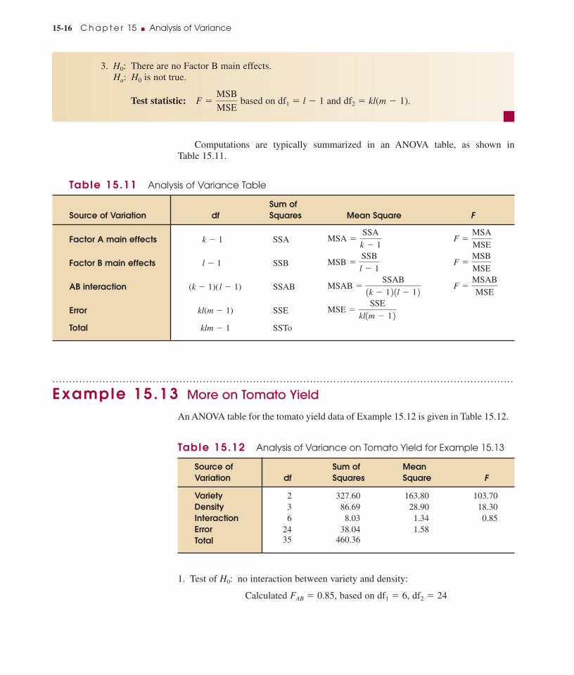
Computations are typically summarized in an ANOVA table, as shown in Table 15.11.

Table 15.11 Analysis of Variance Table

Sum of Source of Variation df Squares Mean Square F

Factor A main effects k � 1 SSA

Factor B main effects l � 1 SSB

AB interaction (k � 1)( l � 1) SSAB

Error kl(m � 1) SSE

Total klm � 1 SSTo

..................... .. .. .. .. .. .. .. .. .. .. .. .. . . . . . . . . . . ...................................................................................

Example 15.13 More on Tomato Yield

An ANOVA table for the tomato yield data of Example 15.12 is given in Table 15.12.

Table 15.12 Analysis of Variance on Tomato Yield for Example 15.13


Variety 2 327.60 163.80 103.70Density 3 86.69 28.90 18.30Interaction 6 8.03 1.34 0.85Error 24 38.04 1.58Total 35 460.36

1. Test of H0: no interaction between variety and density:

Calculated FAB � 0.85, based on df1 � 6, df2 � 24

MSE �SSE

kl1m � 1 2

F �MSAB

MSEMSAB �

SSAB

1k � 1 2 1l � 1 2

F �MSB

MSEMSB �

SSB

l � 1

F �MSA

MSEMSA �

SSA

k � 1


3. H0: There are no Factor B main effects.Ha: H0 is not true.

Test statistic: based on df1 � l � 1 and df2 � kl(m � 1).F �MSB

MSE

15-W4008(online) 2/28/07 6:39 AM Page 15-16

From Appendix Table 6, the smallest value for these df’s is 2.04, so P-value � .10.There is no evidence of interaction, so it is appropriate to carry out further testsconcerning the presence of main effects.

2. Test of H0: Factor A (variety) main effects are absent:

calculated FA � 103.7, based on df1 � 2, df2 � 24

Appendix Table 6 shows that P-value � .001. We therefore reject H0 and concludethat true average yield does depend on variety.

3. Test of H0: Factor B (density) main effects are absent:

calculated FB � 18.3, based on df1 � 3, df2 � 24

Again, P-value � .001, so we reject H0 and conclude that true average yield doesdepend on planting density.

�

After the null hypothesis of no Factor A main effects has been rejected, significantdifferences in Factor A levels can be identified by using a multiple comparisons pro-cedure. In particular, the Tukey–Kramer method described previously can be applied.The quantities are now the sample average responses for levels 1, . . . , kof Factor A, and error df is kl(m � 1). A similar comment applies to Factor B main ef-fects and significant differences in Factor B levels.

� The Case m � 1 . .. . . . . . . . . . . ........................................................................ ............

There is a problem with the foregoing analysis when m � 1 (one observation on eachtreatment). Although we did not give the formula, MSE is an estimate of s2 obtainedby computing a separate sample variance s2 for the m observations on each treatmentand then averaging these kl sample variances. With only one observation on each treat-ment, there is no way to estimate s2 separately from each of the treatments.

One way to proceed is to assume a priori that there is no interaction between fac-tors. This should, of course, be done only when the investigator has sound reasons,based on a thorough understanding of the problem, for believing that the factors con-tribute separately to the response. Having made this assumption, the investigator canthen use what would otherwise be an interaction sum of squares for SSE. The funda-mental identity becomes

SSTo � SSA � SSB � SSE

with the four associated df kl � 1, k � 1, l � 1, and (k � 1)(l � 1).Table 15.13 gives the corresponding ANOVA table. FA is the test statistic for test-

ing the null hypothesis that true average responses are identical for all Factor A levels.FB plays a similar role for Factor B main effects. The analysis of data from a random-ized block experiment in fact assumed no interaction between treatments and blocks. IfSSTr is relabeled SSA and if SSBl is relabeled SSB, the formulas for all sums of squaresgiven in Section 15.3 are valid here.

x1, x2, p , xk


15-W4008(online) 2/28/07 6:39 AM Page 15-17

Table 15.13 ANOVA Table for Two-Factor Experiment with m � 1

Source of Sum of Variation df Squares Mean Square F

Factor A k � 1 SSA

Factor B l � 1 SSB

Error (k � 1)(l � 1) SSE

Total kl � 1 SSTo

..................... .. .. .. .. .. .. .. .. .. .. .. .. . . . . . . . . . . ...................................................................................

Example 15.14 Effect of Soil Type and Pipe Coating on Corrosion

� When metal pipe is buried in soil, it is desirable to apply a coating to retard corro-sion. Four different coatings are under consideration for use with pipe that will ulti-mately be buried in three types of soil. An experiment to investigate the effects ofthese coatings and soils was carried out by first selecting 12 pipe segments and apply-ing each coating to 3 segments. The segments were then buried in soil for a specifiedperiod in such a way that each soil type received one piece with each coating. The re-sulting data (depth of corrosion) and ANOVA table are given in Table 15.14. Assum-ing that there is no interaction between coating type and soil type, let’s test at level .05for the presence of separate Factor A (coating) and Factor B (soil) effects.

Table 15.14 Data and ANOVA Table for Example 15.14

Factor AFactor B (Soil)

Sample(Coating) 1 2 3 Average

1 64 49 50 54.332 53 51 48 50.673 47 45 50 47.334 51 43 52 48.67

Sample average 53.75 47.00 50.00

Source of Sum of Variation df Squares Mean Square F

Factor A 3 83.5 27.8

Factor B 2 91.5 45.8

Error 6 123.3 20.6Total 11 298.3

FB �45.8

20.6� 2.2

FA �27.8

20.6� 1.3

x � 50.25

MSE �SSE

1k � 1 2 1m � 1 2

F �MSB

MSE MSB �

SSB

l � 1

F �MSA

MSE MSA �

SSA

k � 1


Step-by-step technology instructions available online � Data set available online

15-W4008(online) 2/28/07 6:39 AM Page 15-18

� E x e r c i s e s 15.44–15.56

15.44 Many students report that test anxiety affects theirperformance on exams. A study of the effect of anxiety andinstructional mode (lecture versus independent study) ontest performance was described in the article “InteractiveEffects of Achievement Anxiety, Academic Achievement,and Instructional Mode on Performance and Course Atti-tudes” (Home Economics Research Journal [1980]: 216–227). Students classified as belonging to either high- orlow-achievement anxiety groups (Factor A) were assignedto one of the two instructional modes (Factor B). Mean testscores for the four treatments (factor level combinations)are given in the accompanying table. Use these means toconstruct a graph (similar to those of Figure 15.10) of thetreatment sample averages. Does the picture suggest theexistence of an interaction between factors? Explain.

Instructional Mode

Anxiety Independent Group Lecture Group

High 145.8 144.3Low 142.9 144.8

15.45 The behavior of undergraduate students when ex-posed to various odors was examined by the authors of thearticle “Effects of Environmental Odor and Coping Styleon Negative Affect, Anger, Arousal and Escape” (Journalof Applied Social Psychology [1999]: 245–260). The fol-lowing table was constructed using data on reported dis-comfort level (measured on a scale from 1 to 5). Therewere 24 students in each odor–gender combination.

Male FemaleType of Odor

No odor 1.36 1.68Rotten egg 1.83 2.33Skunk 2.42 2.69Cigarette ash 2.74 3.16

xx

a. Construct a graph (similar to those of Figure 15.10)that shows the mean discomfort level on the vertical axis.Mark the four odor categories on the horizontal axis. Thenplot the four means for the males and connect them withline segments. Plot the four means for females and con-nect them with line segments.b. Interpret the interaction plot. Do you think that there isan interaction between gender and type of odor?

15.46 Explain why the individual effects of Factor A orFactor B cannot be interpreted when an AB interaction ispresent.

15.47 The accompanying plot appeared in the article“Group Process-Work Outcome Relationships: A Note onthe Moderating Impact of Self-Esteem” (Academy of Man-agement Journal [1982]: 575–585). The response variablewas tension, a measure of job strain. The two factors ofinterest were peer-group interaction (with two levels—high and low) and self-esteem (also with two levels—highand low).

a. Does this plot suggest an interaction between peergroup interaction and self-esteem? Explain.b. The authors of the article state, “Peer group interactionhad a stronger effect on individuals with lower self-esteemthan on those with higher self-esteem.” Do you agree withthis statement? Explain.

15.48 The following partially completed ANOVA tableapproximately matches summary statistics given in the

Low High

High self-esteem

Low self-esteem

Averageresponse

X

O

O

X


Appendix Table 6 shows that P-value � .10 for both tests. It appears that thetrue average response (amount of corrosion) depends on neither the coating used northe type of soil in which the pipe is buried.

�

. . . . ............................................................ ............ ................................


15-W4008(online) 2/28/07 6:39 AM Page 15-19

article “From Here to Equity: The Influence of Status onStudent Access to and Understanding of Science” (ScienceEducation [1999]: 577–602). The study described in thisarticle attempted to quantify the effect of socioeconomicstatus on learning science. The response variable was“Rate of Talk” (the number of on-task talk speech acts perminute) during group work. Data were also collected onthe variable socioeconomic status (low, middle, high) andthe variable gender (female, male). The author allowed for an interaction between gender and status. Assume thatthere were 12 students at each status–gender level combi-nation, for a total of 72 subjects.


Status 2 14.49Gender 1 .15Interaction 2 .95Error 66 .0120Total 71

a. Fill in the missing numbers in the ANOVA table.b. Is there a significant interaction between status andgender?c. Is there a difference between the mean “Rate of Talk”scores for girls and boys?d. Is there a difference between the mean “Rate of Talk”scores across the three different status groups?

15.49 The article “Experimental Analysis of Prey Selec-tion by Largemouth Bass” (Transactions of the AmericanFisheries Society [1991]: 500–508) gave an ANOVA sum-mary in which the response variable was a certain prefer-ence index, there were three sizes of bass, and there weretwo different species of prey. Three observations weremade for each size–species combination. Sums of squaresfor size, species, and interaction were reported as .088,.048, and .048, respectively, and SSTo � .316. Test therelevant hypotheses using a significance level of .01.

15.50 Is self-esteem related to year in college or to frater-nity membership? The authors of the article “Self-EsteemAmong College Men as a Function of Greek Affiliationand Year in College” (Journal of College Student Develop-ment [1998]: 611–613) interviewed 75 college men whowere members of fraternities and 57 who were not. In ad-dition to Greek status (in a fraternity, not in a fraternity),year in college (freshman, sophomore, junior, senior) was

also noted. Subjects completed a 10-item, self-esteem in-ventory, which was used to compute a self-esteem score.The article reported the following F statistic values from atwo-way ANOVA:

Source F

Greek status 20.53Year 2.59Interaction .70

a. Is there evidence of a significant interaction betweenyear and Greek status?b. Is the main effect for Greek status significant?c. Is the main effect for year significant?

15.51 Three ultrasonic devices (Factor A, with levels 20,30, and 40 kHz) were tested for effectiveness under twotest conditions (Factor B, with levels plentiful food supplyand restricted food supply). Daily food consumption wasrecorded for three rats under each factor–level combina-tion for a total of 18 observations. Data compatible withsummary values given in the article “Variables AffectingUltrasound Repellency in Philippine Rats” (Journal ofWildlife Management [1982]: 148–155) were used to obtain the sums of squares given in the accompanyingANOVA table. Complete the table, and use it to test therelevant hypotheses.


Factor A main effects 4206

Factor B main effects 1782

Interaction between Factors A and B

Error 2911

Total 10,846

15.52 The article “Learning, Opportunity to Cheat, andAmount of Reward” (Journal of Experimental Education[1977]: 30–40) described a study to determine the effectsof expectations concerning cheating during a test and per-ceived payoff on test performance. Subjects, students at



15-W4008(online) 2/28/07 6:39 AM Page 15-20

UCLA, were randomly assigned to a particular factor–level combination. Factor A was expectation of opportu-nity to cheat, with levels high, medium, and low. Those inthe high group were asked to study and then recall a list ofwords. For the first four lists, they were left alone in aroom with the door closed, so they could look at the origi-nal list of words if they wanted to. The medium group wasasked to study and recall the list while left alone but withthe door open. For the low group, the experimenter re-mained in the room. For study and recall of a fifth list, theexperimenter stayed in the room for all three groups, thusprecluding any cheating on the fifth list. Score on the fifthtest was the response variable. The second factor (B) un-der study was the perceived payoff, with a high and a lowlevel. The high payoff group was told that if they scoredabove average on the test, they would receive 2 hours ofcredit rather than just 1 hour (subjects were fulfilling acourse requirement by participating in experiments). Thelow group was not given any extra incentive for scoringabove the average. The article gave the following statis-tics: FA � 4.99, FB � 4.81, FAB � 1, error df � 120. Testthe null hypothesis of no interaction between the factors.If appropriate, test the null hypotheses of no Factor A andno Factor B effects. Use a � .05.

15.53 The accompanying (slightly modified) ANOVAtable appeared in the article “An Experimental Test ofMate Defense in an Iguanid Lizard” (Ecology [1991]:1218–1224). The response variable was territory size.

Source of Sum of Variation df Squares

Age 1 .614Sex 1 1.754Interaction 1 .146Error 80 5.624

a. How many age classes were there?b. How many observations were made for each age–sexcombination?c. What conclusions can be drawn about how the factorsaffect the response variable?

15.54 Identification of gender in human skeletons is animportant part of many anthropological studies. An experi-ment conducted to determine whether measurements of thesacrum could be used to determine gender was described inthe article “Univariate and Multivariate Methods for Sexing

the Sacrum” (American Journal of Physical Anthropology[1978]: 103–110). Sacra from skeletons of individuals ofknown race (Factor A, with two levels—Caucasian andblack) and gender (Factor B, with two levels—male and fe-male) were measured and the lengths recorded. Data com-patible with summary quantities given in the article wereused to compute the following: SSA � 857, SSB � 291,SSAB � 32, SSE � 5541, and error df � 36.a. Use a significance level of .01 to test the null hypothe-sis of no interaction between race and gender.b. Using a .01 significance level, test to determinewhether the true average length differs for the two races.c. Using a .01 significance level, test to determine whetherthe true average length differs for males and females.

15.55 The article “Food Consumption and Energy Re-quirements of Captive Bald Eagles” (Journal of WildlifeManagement [1982]: 646–654) investigated mean grossdaily energy intake (the response variable) for differentdiet types (Factor A, with three levels—fish, rabbit, andmallard) and temperatures (Factor B, with three levels).Summary quantities given in the article were used togenerate data, resulting in SSA � 18,138, SSB � 5182,SSAB � 1737, SSE � 11,291, and error df � 36. Con-struct an ANOVA table and test the relevant hypotheses.

15.56 � The effect of three different soil types and threephosphate application rates on total phosphorus uptake(mg) of white clover was examined in the article “A Glass-house Comparison of Six Phosphate Fertilisers” (NewZealand Journal of Experimental Agriculture [1984]: 131–140). Only one observation was obtained for each factor–level combination. Assuming there is no interaction be-tween soil type and application rate, use the accompanyingdata to construct an ANOVA table and to test the null hy-potheses of no main effects due to soil type and of no maineffects due to application rate. Also identify significantdifferences among soil types.

Application Soil typeRate (kgP/ha) Ramiha Konini Wainui

0 1.29 10.42 17.1075 11.73 21.08 23.69

150 17.63 31.37 32.88



15-W4008(online) 2/28/07 6:39 AM Page 15-21

......................................................................................................................................

15.5 Interpreting and Communicating the Results ofStatistical Analyses

The ANOVA procedures introduced in this chapter are used to compare more than twopopulation or treatment means. When a single-factor ANOVA has been used to test thenull hypothesis of equal population or treatment means, the value of the F statistic andthe associated P-value usually are reported. It is also fairly common to see the support-ing calculations summarized in an ANOVA table, although this is not always the case.

� What to Look For in Published Data ................................................................

Here are some questions to ask when you read an article that includes a description ofa single-factor ANOVA:

� Are the assumptions required for the validity of the ANOVA procedure reasonable?Specifically, are the samples independently chosen, or is there random assignmentto treatments? Is it reasonable to think that the population or treatment response dis-tributions are normal in shape? Are the reported sample standard deviations con-sistent with the assumption of equal population or treatment variances?

� What is the P-value associated with the test? Does the P-value lead to rejection ofthe null hypothesis?

� If the ANOVA F test led to rejection of the null hypothesis, was a multiple com-parisons procedure used to identify differences in the means? Are the results ofthe multiple comparisons procedure interpreted properly?

� Are the conclusions drawn consistent with the results of the hypothesis test andthe multiple comparisons procedure? If H0 was rejected, does this indicate practi-cal significance or only statistical significance?

As an example, consider an ANOVA performed by the authors of “PerceivedAge and Attractiveness of Models in Cigarette Advertisements” (Journal of Marketing[1992]: 22–37). The investigators hypothesized that certain cigarette brands aimedtheir advertising at the young and that the average age of readers of magazines inwhich the cigarette ads appeared was not the same for the 12 brands of cigarettes stud-ied. This hypothesis was tested using a single-factor ANOVA. The following ANOVAtable is from the article:


Treatments 11 592.66 53.88 4.13Error 175 2282.98 13.05

Total 186 2875.64

It was reported that the hypothesis of equal mean ages for the 12 brands considered inthe study was rejected (F � 4.13, P-value � .001). This was interpreted as support forthe researchers’ hypothesis that some brands targeted the young. (Does this conclusionnecessarily follow from the result of the ANOVA F test?)


15-W4008(online) 2/28/07 6:39 AM Page 15-22

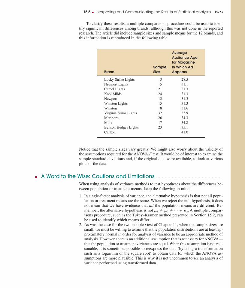
To clarify these results, a multiple comparisons procedure could be used to iden-tify significant differences among brands, although this was not done in the reportedresearch. The article did include sample sizes and sample means for the 12 brands, andthis information is reproduced in the following table:

Average Audience Age for Magazine

Sample in Which Ad Brand Size Appears

Lucky Strike Lights 3 28.5Newport Lights 5 31.1Camel Lights 21 31.3Kool Milds 24 31.3Newport 12 31.3Winston Lights 15 31.3Winston 8 31.6Virginia Slims Lights 32 33.9Marlboro 26 34.3More 17 34.8Benson Hedges Lights 23 35.1Carlton 1 41.0

Notice that the sample sizes vary greatly. We might also worry about the validity ofthe assumptions required for the ANOVA F test. It would be of interest to examine thesample standard deviations and, if the original data were available, to look at variousplots of the data.

� A Word to the Wise: Cautions and Limitations .................................. ............

When using analysis of variance methods to test hypotheses about the differences be-tween population or treatment means, keep the following in mind:

1. In single-factor analysis of variance, the alternative hypothesis is that not all popu-lation or treatment means are the same. When we reject the null hypothesis, it doesnot mean that we have evidence that all the population means are different. Re-member, the alternative hypothesis is not A multiple compar-isons procedure, such as the Tukey–Kramer method presented in Section 15.2, canbe used to identify which means differ.

2. As was the case for the two-sample t test of Chapter 11, when the sample sizes aresmall, we must be willing to assume that the population distributions are at least ap-proximately normal in order for analysis of variance to be an appropriate method ofanalysis. However, there is an additional assumption that is necessary for ANOVA—that the population or treatment variances are equal. When this assumption is not rea-sonable, it is sometimes possible to reexpress the data (by using a transformationsuch as a logarithm or the square root) to obtain data for which the ANOVA as-sumptions are more plausible. This is why it is not uncommon to see an analysis ofvariance performed using transformed data.

m1 m2 p mk.

15.5 � Interpreting and Communicating the Results of Statistical Analyses 15-23

15-W4008(online) 2/28/07 6:39 AM Page 15-23

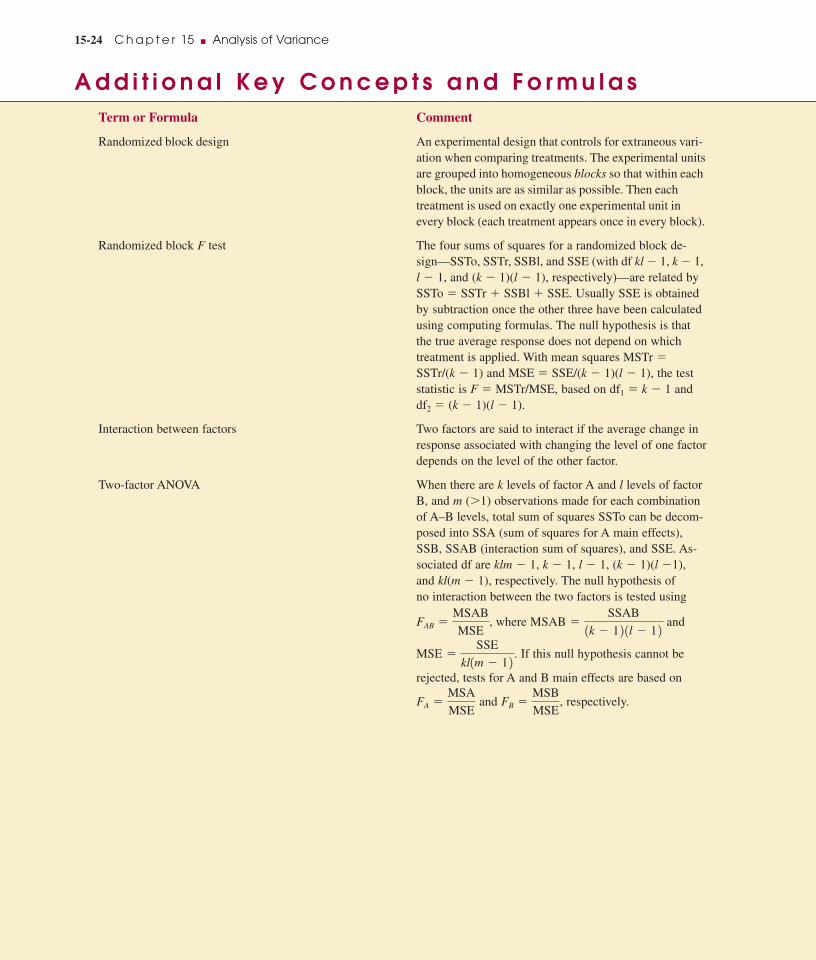
A d d i t i o n a l K e y C o n c e p t s a n d F o r m u l a sTerm or Formula Comment

Randomized block design An experimental design that controls for extraneous vari-ation when comparing treatments. The experimental unitsare grouped into homogeneous blocks so that within eachblock, the units are as similar as possible. Then eachtreatment is used on exactly one experimental unit inevery block (each treatment appears once in every block).

Randomized block F test The four sums of squares for a randomized block de-sign—SSTo, SSTr, SSBl, and SSE (with df kl � 1, k � 1,l � 1, and (k � 1)(l � 1), respectively)—are related bySSTo � SSTr � SSBl � SSE. Usually SSE is obtainedby subtraction once the other three have been calculatedusing computing formulas. The null hypothesis is thatthe true average response does not depend on whichtreatment is applied. With mean squares MSTr �SSTr/(k � 1) and MSE � SSE/(k � 1)(l � 1), the teststatistic is F � MSTr/MSE, based on df1 � k � 1 anddf2 � (k � 1)(l � 1).

Interaction between factors Two factors are said to interact if the average change inresponse associated with changing the level of one factordepends on the level of the other factor.

Two-factor ANOVA When there are k levels of factor A and l levels of factorB, and m (�1) observations made for each combinationof A–B levels, total sum of squares SSTo can be decom-posed into SSA (sum of squares for A main effects),SSB, SSAB (interaction sum of squares), and SSE. As-sociated df are klm � 1, k � 1, l � 1, (k � 1)(l �1),and kl(m � 1), respectively. The null hypothesis of no interaction between the two factors is tested using

where and

. If this null hypothesis cannot be

rejected, tests for A and B main effects are based on

and respectively.FB �MSB

MSE,FA �

MSA

MSE

MSE �SSE

kl1m � 1 2

MSAB �SSAB

1k � 1 2 1l � 1 2FAB �MSAB

MSE,


15-W4008(online) 2/28/07 6:39 AM Page 15-24

C h a p t e r 1 5 A p p e n d i x : A N O VA C o m p u t a t i o n s

Single-Factor ANOVA

Let T1 denote the sum of the observations in the sample from the first population ortreatment, and let T2, . . . , Tk denote the other sample totals. Also let T represent thesum of all N observations—the grand total—and

Then

................... .. .. .. .. .. .. .. .. .. .. .. .. . . . . . . . . . . .....................................................................................

Example 15A.1Treatment 1 4.2 3.7 5.0 4.8 T1 � 17.7 n1 � 4Treatment 2 5.7 6.2 6.4 T2 � 18.3 n2 � 3Treatment 3 4.6 3.2 3.5 3.9 T3 � 15.2 n3 � 4

T � 51.2 N � 11

�

Randomized Block Experiment

Let T1, T2, . . . , Tk denote the treatment totals and B1, B2, . . . , Bl represent the blocktotals. Also, let T be the grand total of all kl observations and

CF � correction factor �T2

kl

SSE � SSTo � SSTr � 118.1 � 9.40 � 2.41

SSTo � aall N obs.

x2 � CF � 14.2 2 2 � 13.7 2 2 � p � 13.9 2 2 � 238.31 � 11.81

� 9.40

�117.7 2 2

4�118.3 2 2

3�115.2 2 2

4� 238.31

SSTr �T

21

n1�

T 22

n2� p �

T 2k

nk� CF

CF � correction factor �T

2

N�151.2 2 2

11� 238.31

SSE � SSTo � SSTr

SSTr �T2

1

n1�

T22

n2� p �

T2k

nk� CF

SSTo � aall N obs.

x2 � CF

CF � correction factor �T2

N

Chapter 15 Appendix � ANOVA Computations 15-25

15-W4008(online) 2/28/07 6:39 AM Page 15-25

Then

..................... .. .. .. .. .. .. .. .. .. .. .. .. . . . . . . . . . . ...................................................................................

Example 15.A2

Block

Treatment 1 2 3 4

1 4.2 3.7 5.0 4.8 T1 � 17.72 5.2 4.5 6.7 5.4 T2 � 21.83 3.4 3.2 5.1 3.9 T3 � 55.1

B1 � 12.8 B2 � 11.4 B3 � 16.8 B4 � 14.1 T � 55.1

�

SSE � SSTo � SSTr � SSBl � 10.73 � 4.97 � 5.28 � 0.48


x2 � CF � 14.2 2 2 � p � 13.9 2 2 � 253.00 � 10.73

� 5.28

�1

3 3 112.8 2 2 � 111.4 2 2 � 116.8 2 2 � 114.1 2 2 4 � 253.00

SSBl �1

k 3B

21 � B

22 � p � B

2l 4 � CF

� 4.97

�1

4 3 117.7 2 2 � 121.8 2 2 � 115.6 2 2 4 � 253.00

SSTr �1

l 3T

21 � T

22 � p � T

2k 4 � CF

CF � correction factor �T

2

kl�155.1 2 213 2 14 2 �

3036.01

12� 253.00

SSE � SSTo � SSTr � SSBl

SSBl �1

k 3B

21 � B

22 � p � B

2l 4 � CF

SSTr �1

l 3T

21 � T2

2 � p � T 2k 4 � CF


x2 � CF


15-W4008(online) 2/28/07 6:39 AM Page 15-26

15.57 A study was carried out to compare aptitudes andachievements of three different groups of college students(“A Comparison of Three Groups of Academically At-RiskCollege Students,” Journal of College Student Develop-ment [1995]: 270–279):1. Students diagnosed as learning disabled2. Students who identified themselves as learning disabled3. Students who were low achieversThe Scholastic Abilities Test for Adults was given to eachstudent. Consider the following summary data on writingcomposition score:

n1 � 30 n2 � 30 n3 � 30� 9.40 � 11.63 � 11.00

SSE � 749.85

Does it appear that population mean score is not the samefor the three types of students? Carry out a test of hypo-thesis. Does your conclusion depend on whether a signifi-cance level of .05 or .01 is used?

15.58 Most large companies have established grievanceprocedures for their employees. One question of interestto employers is why certain groups within a companyhave higher grievance rates than others. The study de-scribed in the article “Grievance Rates and Technology”(Academy of Management Journal [1979]: 810–815) dis-tinguished four types of jobs. These types were labeledapathetic, erratic, strategic, and conservative. Suppose thata total of 52 work groups were selected (13 of each type),and a measure of grievance rate was determined for eachone. Here are the resulting values:

Group Apathetic Erratic Strategic Conservative

Sample mean 2.96 5.05 8.74 4.91

In addition, SSTo � 682.10 and SSE � 506.19. Test atsignificance level .05 to see whether true average griev-ance rate depends on the type of job. If appropriate, usethe T–K method to identify significant differences amongjob types.

x

x3x2x1

15.59 � The results of a study on the effectiveness of linedrying on the smoothness and stiffness of fabric was sum-marized in the article “Line-Dried vs. Machine-Dried Fab-rics: Comparison of Appearance, Hand, and ConsumerAcceptance” (Home Economics Research Journal [1984]:27–35). Smoothness scores were given for nine differenttypes of fabric and five different drying methods—(1) ma-chine dry, (2) line dry, (3) line dry followed by 15-mintumble, (4) line dry with softener, and (5) line dry with airmovement—as given in the accompanying table. Using a.05 significance level, test to see whether there is a differ-ence in the true mean smoothness scores for the dryingmethods. (There may be “extraneous” variation due to dif-ferent fabrics.)

Drying Method

Fabric 1 2 3 4 5

Crepe 3.3 2.5 2.8 2.5 1.9Doubleknit 3.6 2.0 3.6 2.4 2.3Twill 4.2 3.4 3.8 3.1 3.1Twill mix 3.4 2.4 2.9 1.6 1.7Terry 3.8 1.3 2.8 2.0 1.6Broadcloth 2.2 1.5 2.7 1.5 1.9Sheeting 3.5 2.1 2.8 2.1 2.2Corduroy 3.6 1.3 2.8 1.7 1.8Denim 2.6 1.4 2.4 1.3 1.6

15.60 In many countries, grains and cereals are the pri-mary food source. The authors of the article “MineralContents of Cereal Grains as Affected by Storage and In-sect Infestation” (Journal of Stored Products Research[1992]: 147–151) investigated the effects of storage periodon the mineral content of maize. Four storage periods wereconsidered: 0 months (no storage), 1 month, 2 months, and4 months. Twenty-four containers of maize were randomlydivided into four groups of six each. The iron content(mg/100 g dry weight) of the first group of six was mea-sured immediately (0 months of storage), the second sixwere measured after 1 month in storage, etc. The follow-

� Chapter Review Exercises 15-27

C h a p t e r R e v i e w E x e r c i s e s 1 5 . 5 7 – 1 5 . 6 8

Know exactly what to study! Take a pre-test and receive your Personalized Learning Plan.


15-W4008(online) 2/28/07 6:39 AM Page 15-27

ing summary quantities are consistent with information inthe article:

Storage Period s 2

0 4.923 .0001071 4.923 .0000672 4.917 .0001474 4.902 .000057

a. Use a test with a � .05 to decide whether true averageiron content is the same for all four storage periods.b. If appropriate, carry out a multiple comparison analysis.

15.61 � Controlling a filling operation with multiple fill-ers requires adjustment of the individual units. Data re-sulting from a sample of size 5 from each pocket of a12-pocket filler were given in the article “Evaluating Vari-ability of Filling Operations” (Food Technology [1984]:51–55). Data for the first five pockets are given in theaccompanying table.

Pocket Fill (oz)

1 10.2 10.0 9.8 10.4 10.02 9.9 10.0 9.9 10.1 10.03 10.1 9.9 9.8 9.9 9.74 10.0 9.7 9.9 9.7 9.65 10.2 9.8 9.9 9.7 9.8

Use the ANOVA F test to determine whether the null hy-pothesis of no difference in the mean fill weight of thefive pockets can be rejected. If so, use an appropriate tech-nique to determine where the differences lie.

15.62 � This problem requires the use of a computerpackage. The effect of oxygen concentration on fermenta-tion end products was examined in the article “Effects of Oxygen on Pyruvate Formate Lyase in Situ and SugarMetabolism of Streptococcus mutans and Streptococcussamguis” (Infection and Immunity [1985]: 129–134). Fouroxygen concentrations (0, 46, 92, and 138 mM) and twotypes of sugar (galactose and glucose) were used. The accompanying table gives two observations on amount of ethanol produced (mmol/mg) for each sugar–oxygen

x

concentration combination. Construct an ANOVA tableand test the relevant hypotheses.

Oxygen Concentration Galactose Glucose

0 .59, .30 .25, .0346 .44, .18 .13, .0292 .22, .23 .07, .00

138 .12, .13 .00, .01

15.63 The accompanying ANOVA table is from the article“Bacteriological and Chemical Variations and Their Inter-Relationships in a Slightly Polluted Water-Body” (Interna-tional Journal of Environmental Studies [1984]: 121–129).A water specimen was taken every month for a year ateach of 15 designated locations on the Lago di Piedilucoin Italy. The ammonia-nitrogen concentration was deter-mined for each specimen and the resulting data analyzedusing a two-way ANOVA. The researchers were willing to assume that there was no interaction between the twofactors location and month. Complete the given ANOVAtable, and use it to perform the tests required to determinewhether the true mean concentration differs by location or by month of year. Use a .05 significance level for bothtests.


Location 0.6Month 11 2.3ErrorTotal 179 6.4

15.64 The water absorption of two types of mortar usedto repair damaged cement was discussed in the article“Polymer Mortar Composite Matrices for Maintenance-Free, Highly Durable Ferrocement” (Journal of Ferro-cement [1984]: 337–345). Specimens of ordinary cementmortar (OCM) and polymer cement mortar (PCM) weresubmerged for varying lengths of time (5, 9, 24, or 48 hr)and water absorption (% by weight) was recorded. Withmortar type as Factor A (with two levels) and submersionperiod as Factor B (with four levels), three observationswere made for each factor–level combination. Data in-cluded in the article were used to compute the follow-ing sums of squares: SSA � 322.667, SSB � 35.623,



15-W4008(online) 2/28/07 6:39 AM Page 15-28

SSAB � 8.557, SSTo � 372.113. Use this information toconstruct an ANOVA table, and then use a .05 significancelevel to test the appropriate hypotheses.

15.65 Suppose that each observation in a single-factorANOVA data set is multiplied by a constant c (a change inunits; for example, c � 2.54 changes observations frominches to centimeters). How does this affect MSTr, MSE,and the test statistic F? Is this reasonable? Explain.

15.66 � Three different brands of automobile batteries,each one having a 42-month warranty, were included in astudy of battery lifetime. A random sample of batteries ofeach brand was selected and lifetime (in months) was de-termined, resulting in the following data:

Brand 1 45 38 52 47 45 42 43Brand 2 39 44 50 54 48 46 40Brand 3 50 46 43 48 57 44 48

State and test the appropriate hypotheses using a signifi-cance level of .05. Be sure to summarize your calculationsin an ANOVA table.

15.67 Let c1, c2, . . . , ck denote k specified numbers, andconsider the quantity u defined by

A confidence interval for u is then

where the t critical value is based on an error df of N � k.For example, in a study carried out to compare pain re-lievers with respect to true average time to relief, supposethat brands 1, 2, and 3 are nationally available, whereasbrands 4 and 5 are sold only by two large chains of drugstores. An investigator might then wish to consider

u �1

3 m1 �

1

3 m2 �

1

3 m3 �

1

2 m4 �

1

2 m5

� 1t critical value 2BMSE a c21

n1� p �

c2k

nkb

c1x1 � p � ck xk

u � c1m1 � c2 m2 � p � ck

mk

which, in essence, compares the average time to relief ofthe national brands to the average for the house brands.Refer to Exercise 15.66 and suppose that brand 1 is a storebrand and brands 2 and 3 are national brands. Obtain a95% confidence interval for

15.68 � One of the assumptions that underlies the validityof the ANOVA F test is that the population or treatmentresponse variances should be identical re-gardless of whether H0 is true: the assumption of constantvariance across populations or treatments. In some situa-tions, the x values themselves may not satisfy this assump-tion, yet a transformation using some specified mathemat-ical function (for example, taking the logarithm or thesquare root) will give observations that have (approxi-mately) constant variance. The ANOVA F test can then be applied to the transformed data. When observations aremade on a counting variable (x � number of something),statisticians have found that taking the square root willfrequently “stabilize the variance.” In an experiment tocompare the quality of four different brands of videotape,cassettes of a specified length were selected, and the num-ber of flaws in each was determined.

Brand 1 10 14 5 12 8Brand 2 17 14 8 9 12Brand 3 13 18 15 18 10Brand 4 14 22 12 16 17

Make a square-root transformation, and analyze the resulting data by using the ANOVA F test at significancelevel .01.

s21, s

22, p , s2

k

u � m1 �1

2 m2 �

1

2 m3

� Chapter Review Exercises 15-29


Are you ready? Take yourexam-prep post-test now.

Do you need a live tutor for homework problems?

15-W4008(online) 2/28/07 6:39 AM Page 15-29

Answers to SelectedOdd-NumberedExercises

Chapter 15

15.35 A randomized block experiment was used to control the factorvalue of house, which definitely affects the assessors’ appraisals. If acompletely randomized experiment had been done, then there wouldhave been danger of having the assessors appraising houses which werenot of similar value. Therefore, differences between assessors would bepartly due to the fact that the homes were dissimilar, as well as to differ-ences in the appraisals made.15.37 a.

Source of Degrees of Sum of MeanVariation Freedom Squares Square F

Treatments 2 11.7 5.85 0.37Blocks 4 113.5 28.375Error 8 125.6 15.7Total 14 250.8

b. F � 0.37, P-value � 0.10, fail to reject H0

15.39 a. Other environmental factors (amount of rainfall, number ofdays of cloudy weather, average daily temperature, etc.) vary from yearto year. Using a randomized complete block helps control for variation inthese other factors. b. F � 15.03, 0.01 � P-value � 0.05, reject H0

c.

Application Rate 1 2 3Mean 138.33 152.33 156.33

15.41 F � 0.868, P-value � 0.10, fail to reject H0

15.43 F � 79.4, P-value � 0.001, reject H0

15.45 b. The lines are very nearly parallel. The plot does not show evi-dence of an interaction between gender and type of odor.

15.47 a. The plot does suggest an interaction between peer group andself-esteem. b. The change in the average response is greater for thelow self-esteem group than it is for the high self-esteem group, whenchanging from low to high peer group. The authors are correct in theirstatement.15.49 Test for interaction: F � 2.18, P-value � 0.10, fail to reject H0; test for main effect for size: F � 4.00, 0.01 � P-value � 0.05, fail to reject H0; test for main effect for species: F � 4.36, 0.05 � P-value � 0.10, fail to reject H0

15.51 Test for interaction: F � 4.01, 0.01 � P-value � 0.05, with a � .05 reject H0. Since there is a significant interaction, tests for maineffects are not appropriate.15.53 a. 2 b. 21 c. Test for interaction: F � 2.08, P-value � 0.10,fail to reject H0; test for main effect for age: F � 8.73, 0.001 � P-value� 0.01, reject H0; test for main effect for sex: F � 24.95, P-value �0.001, reject H0

15.55 Test for interaction: F � 1.38, P-value � 0.10, fail to reject H0; test for main effect for diet: F � 28.92, P-value � 0.001, reject H0; test for main effect for temperature: F � 8.26, P-value � 0.001,reject H0

15.57 F � 4.60, 0.01 � P-value � 0.05, reject H0 for a � .05 but notfor a � .01.15.59 F � 36.7, P-value � 0.001, reject H0

15.61 F � 2.24, P-value � 0.100, fail to reject H0

15.63 Test for location effect: F � 1.89, 0.01 � P-value � 0.05, rejectH0; test for month effect: F � 9.20, P-value � 0.001, reject H0

15.65 MSTr and MSE are both multiplied by a factor of c 2, but the F statistic is unchanged. It is reasonable that the test statistic would notdepend on the unit of measurement. 15.67 (�7.0337, 2.3187)

15-30

15-W4008(online) 2/28/07 6:39 AM Page 15-30

15.3 The F Test for a Randomized Block Experiment The F Test for a Randomized Block Experiment ......

Documents

Transcript of 15.3 The F Test for a Randomized Block Experiment The F Test for a Randomized Block Experiment ......