1/51

Rejection Based Face Detection

Michael Elad*

Scientific Computing and Computational Mathematics

Stanford University

(Gates 282, phone: 723-7685, email: elad@sccm.stanford.edu)

May 13th, 2002

* Collaboration with Y. Hel-Or and R. Keshet

2/51

Chapter 1 Chapter 1

Problem DefinitionProblem Definition

3/51

1.1 Requirements

Face Finder

Detect FRONTAL & VERTICAL faces: All spatial position, all scales any person, any expression Robust to illumination conditions Old/young, man/woman, hair, glasses.

Design Goals: Fast algorithm Accurate (False alarms/ mis-detections)

4/51

1.2 Face Examples

Taken from the ORL Database

5/51

Face Finder

Suspected

Face Positions

Input Image

Classifier

Draw L*L blocks from

each location

1.3 Position & Scale

and in each resolution

layer

Compose a pyramid with 1:f resolution ratio (f=1.2)

6/51

1.4 Classifier?

The classifier gets blocks of fixed size L2 (say 152) pixels, and

returns a decision (Face/Non-Face)

Block of pixels

Decision

HOW ?

7/51

Chapter 2 Chapter 2

Example-Based Example-Based ClassificationClassification

8/51

2.1 Definition

A classifier is a parametric (J parameters) function C(Z,θ) of the

form

Example: For blocks of 4 pixels Z=[z1,z2,z3,z4],

we can assume that C(Z) is obtained by

C(Z, θ)=sign{θ0 +z1 θ1+ z2 θ2+ z3 θ3+ z4

θ4}

}1,1{:,ZC JL2

9/51

2.2 Classifier Design

1. What parametric form to use? Linear or non-linear? What kind of non-linear? Etc.

2. Having chosen the parametric form, how do we find appropriate θ ?

In order to get a good quality classifier, we have to answer two questions:

}1,1{:,ZC JL2

10/51

2.3 Complexity

Searching faces in a given scale, for a 1000 by 2000 pixels image, the classifier is applied 2e6 times

THE ALGORITHMS’ COMPLEXITY IS GOVERNED BY THE CLASSIFIER PARAMETRIC

FORM

11/51

2.4 Examples

Collect examples of Faces and Non-Faces { } { }X YN N

k kk 1 k 1Faces: X , Non-Faces: Y

= =

Obviously, we should have NX<<NY

12/51

2.5 Training

The basic idea is to find θ such that

or with few errors only, and with good GENERALIZATION ERROR

1,YC,Nk1

1,XC,Nk1

kY

kX

13/51

2.6 Geometric View

{ } XNk k 1

X=

{ } YNk k 1

Y=

C(Z,θ) is to drawing a separating manifold between the two classes

+1 -1

2L

14/51

Chapter 3 Chapter 3

Linear ClassificationLinear Classification

15/51

3.1 Linear Separation

The Separating manifold is a Hyper-plane

+1

-1

{ } XNk k 1

X=

{ } YNk k 1

Y=

2L

0TZsign,ZC

16/51

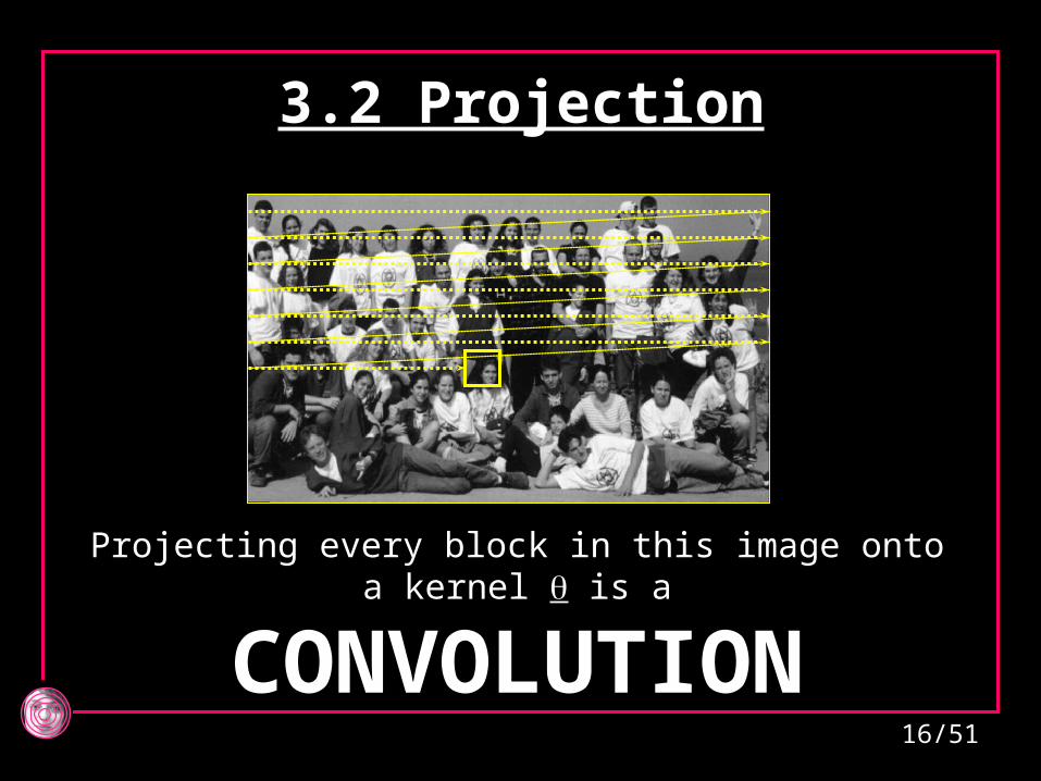
3.2 Projection

Projecting every block in this image onto a kernel

is a CONVOLUTION

17/51

3.3 Linear Operation

False Alarm

Mis- Detection

{ } XNk k 1

X=

TkX θ

0

TkY

YNk k 1

Y

TZ

θ0

18/51

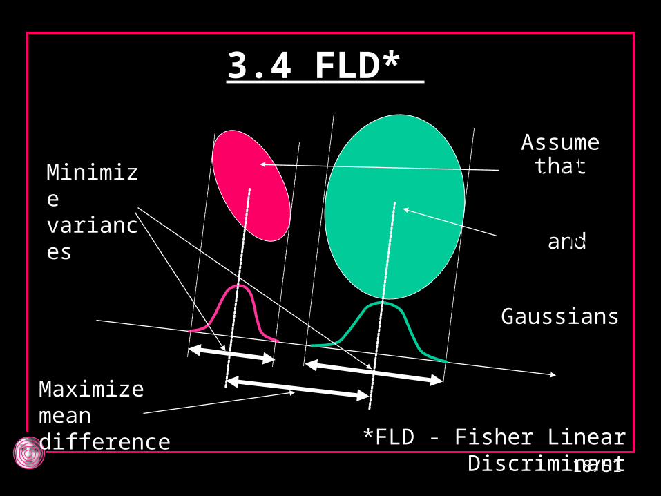
3.4 FLD*

*FLD - Fisher Linear Discriminant

Assume that

and

Gaussians

XNk k 1

X

YNk k 1

Y

Minimize variances

Maximize mean difference

19/51

3.5 Projected Moments

Nk k 1Z

Nk

k 1N T

k kk 1

1M Z

N

1Z M Z M

N

R

T T Tk kz Z m M, r R

20/51

2T T

X Y

T TX Y

M Mf

R R

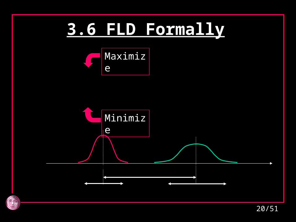
Maximize

Minimize

3.6 FLD Formally

TXM T

YM

TXR T

YR

TTX Y X Y

TX Y

M M M M

R R

21/51

2

T2

T1

Minimize ( )

R

Q

T T T2

2 TT

( )0

Q R R Q RR Q

QQ

3.7 Solution

Generalized Eigenvalue Problem: Rv=Qv

The solution is the eigenvector which

corresponds to the largest eigenvalue

Maximize

22/51

3.8 SVM*

*SVM - Support Vector Machine

Among the many possible solutions, choose the one which Maximizes the minimal distance to the

two example-sets

YNk k 1

Y XNk k 1

X

23/51

3.9 Support Vectors

1. The optimal θ turns out to emerge as the solution of a Quadratic-Programming problem

2. The support vectors are those realizing the minimal distance. Those vectors define the decision function

mindmind

YNk k 1

Y XNk k 1

X

24/51

Linear methods are not suitable

1. Generalize to non-linear Discriminator by either mapping into higher dimensional space, or using kernel functions

2. Apply complex pre-processing on the block

Complicated Classifier!!

3.10 Drawback

25/51

3.11 Previous Work• Rowley & Kanade (1998), Juel & March (96):

Neural Network approach - NL

• Sung & Poggio (1998):

Clustering into sub-groups, and RBF - NL

• Osuna, Freund, & Girosi (1997):

Support Vector Machine & Kernel functions - NL

• Osdachi, Gotsman & Keren (2001):

Anti-Faces method - particular case of our work

• Viola & Jones (2001):

Similar to us (rejection, simplified linear class., features)

26/51

Chapter 4 Chapter 4

Maximal Rejection Maximal Rejection ClassificationClassification

27/51

Faces

Non-Faces

We think of the non-faces as a much richer set and more probable, which may even

surround the faces set

XNk k 1

X

YNk k 1

Y

4.1 Model Assumption

28/51

Find θ1 and two decision levels such that the number of rejected non-faces is maximized

while finding all faces

1 2 1d ,d

4.2 Maximal Rejection

1d

2d

Projected onto θ1

Rejected points

29/51

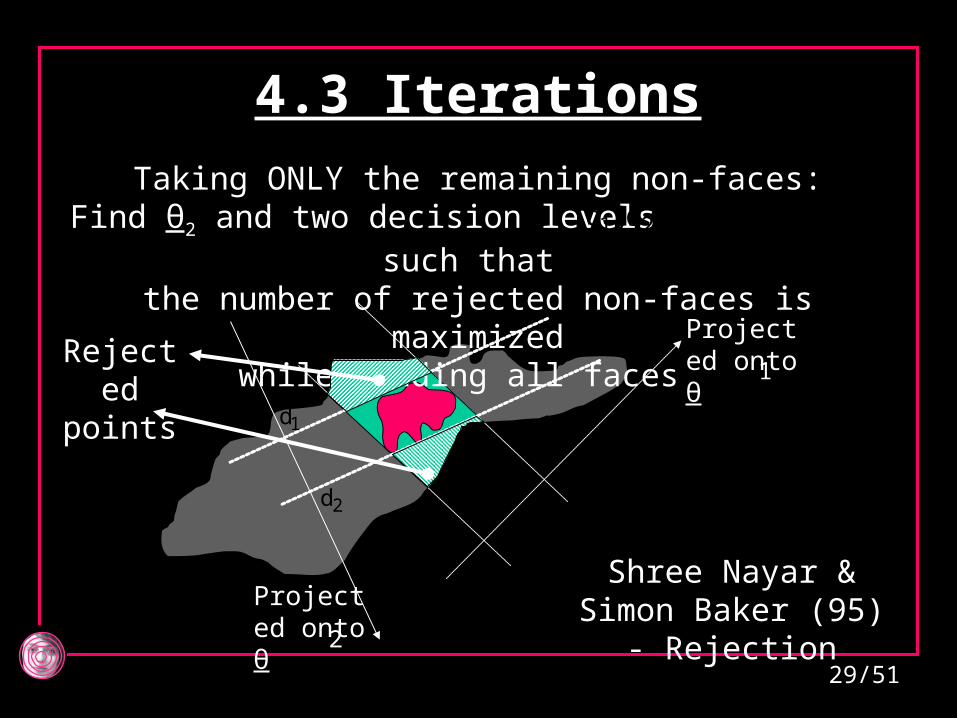
Projected onto θ1

Taking ONLY the remaining non-faces:Find θ2 and two decision levels such that the number of rejected non-faces is maximized

while finding all faces

4.3 Iterations

1 2 2d ,d

Projected onto θ2

1d

2d

Rejected

points

Shree Nayar & Simon Baker (95) -

Rejection

30/51

4.4 Formal Derivation

XNk k 1

X Maximal Rejection

Maximal distance between these two

PDF’s

We need a measure for this distance which will

be appropriate and easy to use

YNk k 1

Y

31/51

Y X

X X

N N 2T Tk j

j 1k 1N N 2T T

k jj 1k 1

X Y

fX X

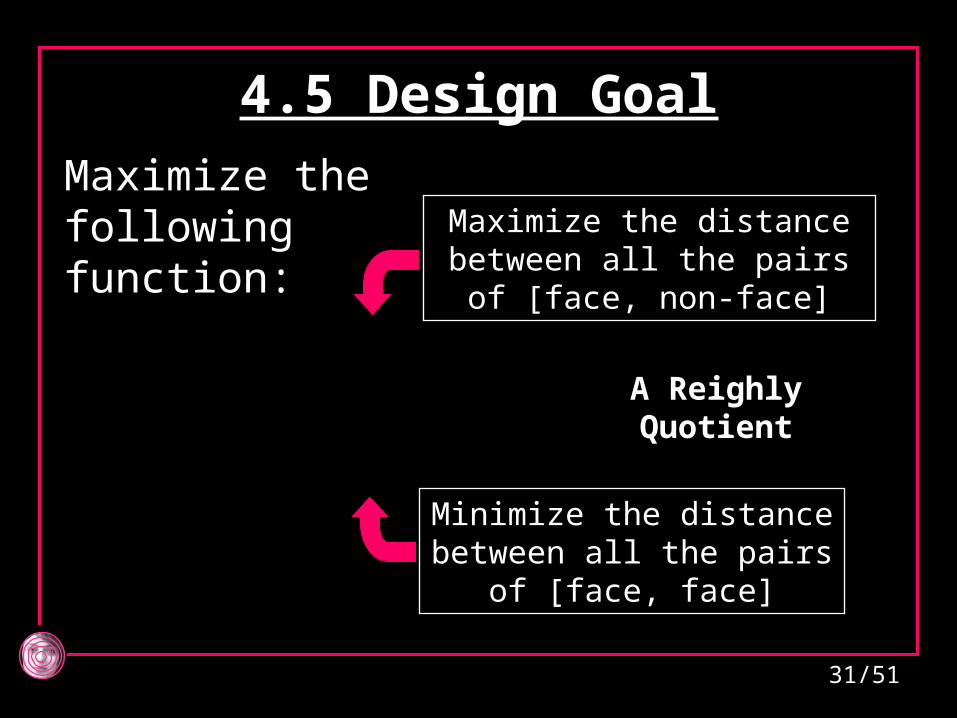
Maximize the following function:

4.5 Design Goal

Maximize the distance between all the pairs of

[face, non-face]

Minimize the distance between all the pairs of

[face, face]

T

TC

R

Q

A Reighly Quotient

32/51

TT

X YX Y X Y

TX

M M M M R Rf

R

4.6 Objective Function

•The expression we got finds the optimal kernel θ in terms of the 1st and the 2nd moments only.

•The solution effectively project all the X examples to a near-constant value, while spreading the Y’s away - θ plays a role of an approximated invariant of the faces

•As in the FLD, the solution is obtained problem is a Generalized Eigenvalue Problem.

33/51

Chapter 5 Chapter 5

MRC in PracticeMRC in Practice

34/51

5.1 General

There are two phases to the algorithm:

2. Testing: Given an image, finding faces in it using the above found kernels and thresholds.

1. Training:Computing the projection kernels, and their thresholds. This process is done ONCE and off line

35/51

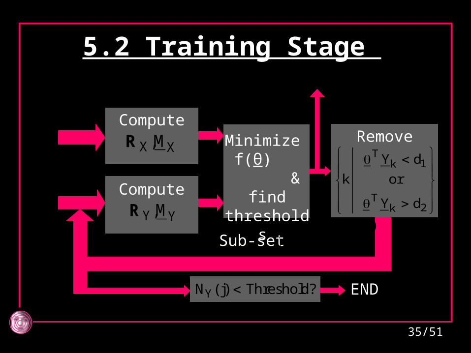
1 2 j,d ,d

T1k

T2k

Y d

k or

Y d

Remove

Sub-set YN (j 1)j 1k k 1

Y

YN (j) Threshold? END

5.2 Training Stage

XNk k 1

X Compute

X X,MR

YN (0)0k

k 1Y

Compute

Y Y,MR

Minimize f(θ)

& find thresholds

36/51

Is value in1 2 j

d ,d

No more Kernels Fac

e

5.3 Testing Stage

Yes

No

Non Face

j j 1

Project onto the

next Kernel

J1 2 j 1

,d ,d

37/51

Original yellow set contains 10000 points

875 false-

alarms

1 136 false-

alarms

3

35 false-

alarms

637 false-

alarms

566 false-

alarms

4

178 false-

alarms

2

5.5 2D Example

38/51

• The discriminated zone is a parallelogram. Thus, if the faces set is non-convex, zero false alarm is impossible!!Solution: Second Layer

• Even if the faces-set is convex, convergence to zero false-alarms is not guaranteed.Solution: Clustering

5.6 Limitations

39/51

5.7 Convexity?

Can we assume that the Faces set is convex?

- We are dealing with a low-resolution representation of the faces

- We are dealing with frontal and vertical faces only

40/51

Chapter 6 Chapter 6

Pre-ProcessingPre-Processing

No time ? Press here

41/51

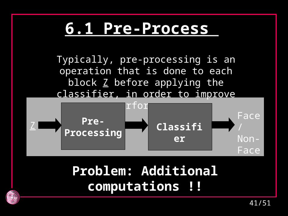
Typically, pre-processing is an operation that is done to each block Z before applying the classifier, in order to

improve performance

Classifier

Pre-Processin

g

ZFace/Non-Face

Problem: Additional computations !!

6.1 Pre-Process

42/51

Option: Acquire many faces with varying types of illuminations, and use these in order to train the system

6.2 Why Pre-Process

Example: Assume that we would like our detection algorithm to be robust to the illumination conditions system

Alternative: Remove (somehow) the effect of the varying illumination, prior to the application of the detection algorithm – Pre-process!

43/51

If the pre-processing is linear (P·Z):

T

1 2d PZ d Face C P ZOtherwise Non-Face

The pre-processing is performed on the Kernels ONCE, before the testing !!

6.3 Linear Pre-Process

TT1 2d P Z d Face

Otherwise Non-Face

44/51

1. Masking to disregard irrelevant pixels.

2. Subtracting the mean to remove sensitivity to brightness changes. Can do more complex things, such as masking

some of the DCT coefficients, which results with reducing sensitivity to lighting conditions,

noise, and more ...

6.4 Possibilities

45/51

Chapter 7 Chapter 7

Results & ConclusionsResults & Conclusions

46/51

7.1 Details • Kernels for finding faces (15·15) and eyes

(7·15).

• Searching for eyes and faces sequentially - very efficient!

• Face DB: 204 images of 40 people (ORL-DB after some screening). Each image is also rotated 5 and vertically flipped - to produce 1224 Face images.

• Non-Face DB: 54 images - All the possible positions in all resolution layers and vertically flipped - about 40·106 non-face images.

• Core MRC applied (no fancy improvements).

47/51

7.2 Results - 1

Out of 44 faces, 10 faces are undetected, and 1 false alarm

(the undetected faces are circled - they are either rotated or shadowed)

48/51

All faces detected with no false alarms

7.3 Results - 2

49/51

7.4 Results - 3

All faces detected with 1 false alarm(looking closer, this false alarm can be considered

as face)

50/51

7.5 Complexity

• A set of 15 kernels - the first typically removes about 90% of the pixels from further consideration. Other kernels give a rejection of 50%.

• The algorithm requires slightly more that one convolution of the image (per each resolution layer).

• Compared to state-of-the-art results:• Accuracy – Similar to (slightly inferior in FA) to Rowley

and Viola. • Speed – Similar to Viola – much faster (factor of ~10)

compared to Rowley.

51/51

7.6 Conclusions

• MRC: projection onto pre-trained kernels, and thresholding. The process is a rejection based discrimination.

• MRC is simple to apply, with promising results for face-detection in images.

• Further work is required to implement this method and tune its performance.

• If the face set is non-convex (e.g. faces in all angles), MRC can serve as a pre-processing for more complex algorithms.

• More details – http://www-sccm.stanford.edu/~elad

52/51

Chapter 8 Chapter 8

AppendicesAppendices

53/51

8.1 Scale-Invariant

20

1 0 x x2x

2 20 x x

2x

D ,P P dr

m r

r

xP

0

Same distance for

xP

0

xP

0

54/51

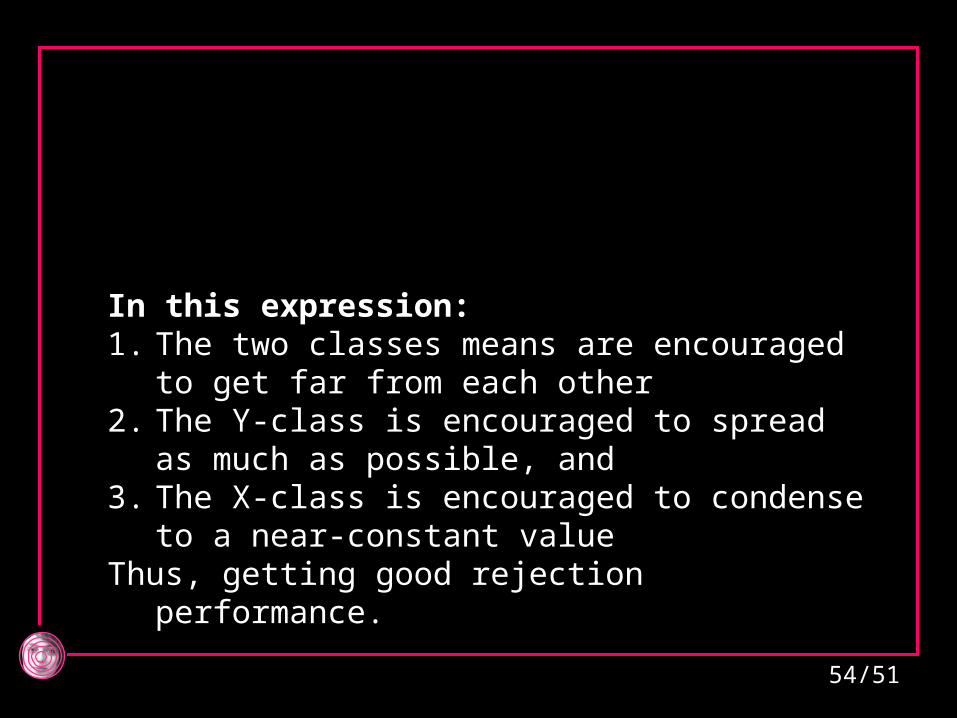
TT

X YX Y X Y

TX

M M M M R Rf

R

In this expression:1. The two classes means are encouraged to

get far from each other 2. The Y-class is encouraged to spread as

much as possible, and 3. The X-class is encouraged to condense to a

near-constant valueThus, getting good rejection performance.

55/51

8.2 Counting Convolutions

6.08.1

9.02.1

99.01~

235.0k112k

1k

• Assume that the first kernel rejection is 0<<1 (I.e. of the incoming blocks are rejected).

• Assume also that the other stages rejection rate is 0.5.

• Then, the number of overall convolutions per pixel is given by

56/51

8.3 Different Analysis 1If the two PDF’s are

assumed Gaussians, their KL distance is

given by

2 2 2

x y x yKL x y 2

x

x

y

(m m ) r rD P ,P

2r

rln 1

r

And we get a similar expression

XNk k 1

X

YNk k 1

Y

57/51

This distance is asymmetric !! It describes the average distance between points of Y to the X-PDF,

PX().

Define a distance between a point and a PDF by

20

1 0 x x2x

2 20 x x

2x

D ,P P dr

m r

r

xP

0

2 2 2

x y x y2 x y 1 y 2

x

(m m ) r rD P ,P D ,Px( ) P ( )d

r

8.4 Different Analysis 2

58/51

2 2 2 2 2 2

x y x y x y x y3 x y 2 2

x y

(m m ) r r (m m ) r rD P ,P P(Y) P(X)

r r

In the case of face detection in images we have

P(X)<<P(Y)

2 2 2x y x y

2x

(m m ) r r

r

We should Maximize

59/51

8.5 Relation to Fisher

2y

2y

2x

2yx

2x

2y

2x

2yx

r

rrmm)X(P

r

rrmm)Y(P

In the general case we maximize the distance

The distance of the Y points to the X-

distribution

The distance of the X points to the Y-

distribution

If P(X)=P(Y)=0.5 we maximize

2y

2y

2x

2yx

2x

2y

2x

2yx

r

rrmm

r

rrmm

60/51

Instead of maximizing the sum

2y

2y

2x

2yx

2x

2y

2x

2yx

r

rrmm

r

rrmm

Minimize the inverse of the two expressions (the inverse represent the

proximity)

2yx

2y

2x

2y

2x

2yx

2y

2y

2x

2yx

2x

mm

rrMin

rrmm

r

rrmm

rMin

61/51

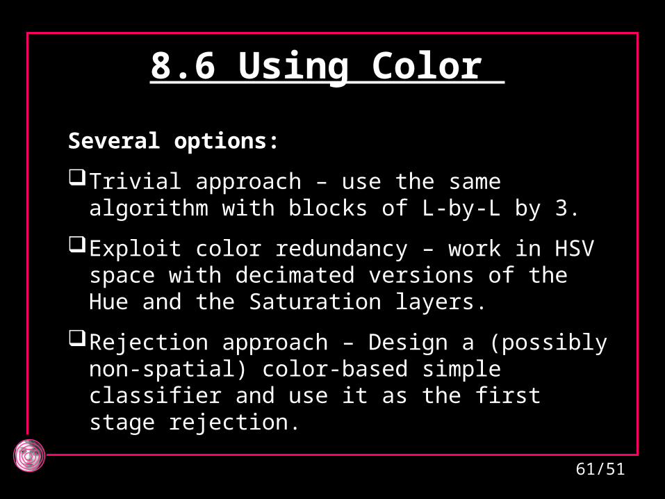
8.6 Using Color

Several options:

Trivial approach – use the same algorithm with blocks of L-by-L by 3.

Exploit color redundancy – work in HSV space with decimated versions of the Hue and the Saturation layers.

Rejection approach – Design a (possibly non-spatial) color-based simple classifier and use it as the first stage rejection.

62/51

8.7 2D-Rotated Faces Frontal

& Vertical

Face Detecto

r

Pose Estimatio

n and Alignment

Input block

Face/Non-Face

Remarks:

1. A set of rotated kernels can be used instead of actually rotating the input block

2. Estimating the pose can be done with a relatively simple system (few convolutions).

63/51

8.8 3D-Rotated Faces A possible solution:

1. Cluster the face-set to same-view angle faces and design a Final classifier for each group using the rejection approach

2. Apply a pre-classifier for fast rejection at the beginning of the process.

3. Apply a mid-classifier to map to the appropriate cluster with the suitable angle

Mid-clas. For

Angle

Crude Rejection

Input block

Face/Non-Face

Final Stage

64/51

8.9 Faces vs. Targets Treating other targets can be done using the

same concepts of

Treatment of scale and location

Building and training sets

Designing a rejection based approach (e.g. MRC)

Boosting the resulting classifier

The specific characteristics of the target in mind could be exploited to fine-tune and improve the above general tools.

65/51

8.10 Further Improvements

• Pre-processing – linear kind does not cost

• Regularization – compensating for shortage in examples

• Boosted training – enrich the non-face group by finding false-alarms and train on those again

• Boosted classifier – Use the sequence of weak-classifier outputs and apply yet another classifier on them –use ada-boosting or simple additional linear classifier

• Constrained linear classifiers for simpler classifier

• Can apply kernel methods to extend to non-linear version

66/51

8.11 Possible Extensions

• Relation to Boosting and Ada-Boosting algorithms,

• Bounding the rejection rate, • Treating non-convex inner classes:

– Non-dyadic decision tree,– Sub-clustering of the inner-class,– Kernel functions,– Combine boosting and MRC.

• Replacing the target-functional for better rejection performance – SVM-like approach.