15 Embedding Finite Metric Spaces into Normed Spacessuri/cs235/MatousekMetric.pdf · 15 Embedding...

15

Embedding Finite MetricSpaces into Normed Spaces

15.1 Introduction: Approximate Embeddings

We recall that a metric space is a pair (X, !), where X is a set and !: X!X "[0,#) is a metric, satisfying the following axioms: !(x, y) = 0 if and only ifx = y, !(x, y) = !(y, x), and !(x, y) + !(y, z) $ !(x, z).

A metric ! on an n-point set X can be specified by an n!n matrix ofreal numbers (actually

!n2

"numbers su!ce because of the symmetry). Such

tables really arise, for example, in microbiology: X is a collection of bacterialstrains, and for every two strains, one can obtain their dissimilarity, whichis some measure of how much they di"er. Dissimilarity can be computedby assessing the reaction of the considered strains to various tests, or bycomparing their DNA, and so on.1 It is di!cult to see any structure in alarge table of numbers, and so we would like to represent a given metricspace in a more comprehensible way.

For example, it would be very nice if we could assign to each x % X a pointf(x) in the plane in such a way that !(x, y) equals the Euclidean distance off(x) and f(y). Such representation would allow us to see the structure of themetric space: tight clusters, isolated points, and so on. Another advantagewould be that the metric would now be represented by only 2n real numbers,the coordinates of the n points in the plane, instead of

!n2

"numbers as be-

fore. Moreover, many quantities concerning a point set in the plane can becomputed by e!cient geometric algorithms, which are not available for anarbitrary metric space.

1 There are various measures of dissimilarity, and not all of them yield a metric,but many do.

366 Chapter 15: Embedding Finite Metric Spaces into Normed Spaces

This sounds very good, and indeed it is too good to be generally true: Itis easy to find examples of small metric spaces that cannot be represented inthis way by a planar point set. One example is 4 points, each two of themat distance 1; such points cannot be found in the plane. On the other hand,they exist in 3-dimensional Euclidean space.

Perhaps less obviously, there are 4-point metric spaces that cannot berepresented (exactly) in any Euclidean space. Here are two examples:

The metrics on these 4-point sets are given by the indicated graphs; that is,the distance of two points is the number of edges of a shortest path connectingthem in the graph. For example, in the second picture, the center has distance1 from the leaves, and the mutual distances of the leaves are 2.

So far we have considered isometric embeddings. A mapping f : X " Y ,where X is a metric space with a metric ! and Y is a metric space witha metric ", is called an isometric embedding if it preserves distances, i.e.,if "(f(x), f(y)) = !(x, y) for all x, y % X . But in many applications weneed not insist on preserving the distance exactly; rather, we can allow somedistortion, say by 10%. A notion of an approximate embedding is capturedby the following definition.

15.1.1 Definition (D-embedding of metric spaces). A mapping f : X "Y , where X is a metric space with a metric ! and Y is a metric space witha metric ", is called a D-embedding, where D $ 1 is a real number, if thereexists a number r > 0 such that for all x, y % X ,

r · !(x, y) & "(f(x), f(y)) & D · r · !(x, y).

The infimum of the numbers D such that f is a D-embedding is called thedistortion of f .

Note that this definition permits scaling of all distances in the same ratior, in addition to the distortion of the individual distances by factors between1 and D. If Y is a Euclidean space (or a normed space), we can rescale theimage at will, and so we can choose the scaling factor r at our convenience.

Mappings with a bounded distortion are sometimes called bi-Lipschitzmappings. This is because the distortion of f can be equivalently defined usingthe Lipschitz constants of f and of the inverse mapping f!1. Namely, if wedefine the Lipschitz norm of f by 'f'Lip = sup{"(f(x), f(y))/!(x, y): x, y %X, x (= y}, then the distortion of f equals 'f'Lip · 'f!1'Lip.

We are going to study the possibility of D-embedding of n-point metricspaces into Euclidean spaces and into various normed spaces. As usual, wecover only a small sample of results. Many of them are negative, showingthat certain metric spaces cannot be embedded too well. But in Section 15.2

15.1 Introduction: Approximate Embeddings 367

we start on an optimistic note: We present a surprising positive result ofconsiderable theoretical and practical importance. Before that, we review afew definitions concerning #p-spaces.

The spaces !p and !dp. For a point x % Rd and p % [1,#), let

'x'p =# d$

i=1

|xi|p%1/p

denote the #p-norm of x. Most of the time, we will consider the case p = 2,i.e., the usual Euclidean norm 'x'2 = 'x'. Another particularly importantcase is p = 1, the #1-norm (sometimes called the Manhattan distance). The#"-norm, or maximum norm, is given by 'x'" = maxi |xi|. It is the limit ofthe #p-norms as p " #.

Let #dp denote the space Rd equipped with the #p-norm. In particular, wewrite #d2 in order to stress that we mean Rd with the usual Euclidean norm.

Sometimes we are interested in embeddings into some space #dp, with pgiven but without restrictions on the dimension d; for example, we can askwhether there exists some Euclidean space into which a given metric spaceembeds isometrically. Then it is convenient to speak about #p, which is thespace of all infinite sequences x = (x1, x2, . . .) of real numbers with 'x'p < #,

where 'x'p =&'"

i=1 |xi|p(1/p

. In particular, #2 is the (separable) Hilbertspace. The space #p contains each #dp isometrically, and it can be shown thatany finite metric space isometrically embeddable into #p can be isometricallyembedded into #dp for some d. (In fact, every n-point subspace of #p can beisometrically embedded into #dp with d &

!n2

"; see Exercise 15.5.2.)

Although the spaces #p are interesting mathematical objects, we will notreally study them; we only use embeddability into #p as a convenient short-hand for embeddability into #dp for some d.

Bibliography and remarks. This chapter aims at providing anoverview of important results concerning low-distortion embeddingsof finite metric spaces. The scope is relatively narrow, and we almostdo not discuss even closely related areas, such as isometric embeddings.A survey with a similar range is Indyk and Matousek [IM04], and onemainly focused on algorithmic aspects is Indyk [Ind01]; however, bothare already outdated because of a very rapid development of the field.

For studying approximate embeddings, it may certainly be help-ful to understand isometric embeddings, and here extensive theory isavailable. For example, several ingenious characterizations of isometricembeddability into #2 can be found in old papers of Schoenberg (e.g.,[Sch38], building on the work of mathematicians like Menger and vonNeumann). A book devoted mainly to isometric embeddings, and em-beddings into #1 in particular, is Deza and Laurent [DL97].


Another closely related area is the investigation of bi-Lipschitzmaps, usually (1+$)-embeddings with $ > 0 small, defined on an opensubset of a Euclidean space (or a Banach space) and being local home-omorphisms. These mappings are called quasi-isometries (the defini-tion of a quasi-isometry is slightly more general, though), and themain question is how close to an isometry such a mapping has to be,in terms of the dimension and $; see Benyamini and Lindenstrauss[BL99], Chapters 14 and 15, for an introduction.

Exercises

1. Consider the two 4-point examples presented above (the square and thestar); prove that they cannot be isometrically embedded into #22. 2 Canyou determine the minimum necessary distortion for embedding into #22?

2. (a) Prove that a bijective mapping f between metric spaces is a D-embedding if and only if 'f'Lip · 'f!1'Lip & D. 1

(b) Let (X, !) be a metric space, |X | $ 3. Prove that the distortionof an embedding f : X " Y , where (Y,") is a metric space, equals thesupremum of the factors by which f “spoils” the ratios of distances; thatis,

sup)"(f(x), f(y))/"(f(z), f(t))

!(x, y)/!(z, t): x, y, z, t % X, x (= y, z (= t

*.

2

15.2 The Johnson–Lindenstrauss Flattening Lemma

It is easy to show that there is no isometric embedding of the vertex setV of an n-dimensional regular simplex into a Euclidean space of dimensionk < n. In this sense, the (n+1)-point set V ) #n2 is truly n-dimensional.The situation changes drastically if we do not insist on exact isometry: Aswe will see, the set V , and any other (n+1)-point set in #n2 , can be almostisometrically embedded into #k2 with k = O(log n) only!

15.2.1 Theorem (Johnson–Lindenstrauss flattening lemma). Let Xbe an n-point set in a Euclidean space (i.e., X ) #2), and let $ % (0, 1]be given. Then there exists a (1+$)-embedding of X into #k2 , where k =O($!2 log n).

This result shows that any metric question about n points in #n2 canbe considered for points in #O(log n)

2 , if we do not mind a distortion of thedistances by at most 10%, say. For example, to represent n points of #n2 ina computer, we need to store n2 numbers. To store all of their distances, weneed about n2 numbers as well. But by the flattening lemma, we can store

15.2 The Johnson–Lindenstrauss Flattening Lemma 369

only O(n log n) numbers and still reconstruct any of the n2 distances witherror at most 10%.

Various proofs of the flattening lemma, including the one below, providee!cient randomized algorithms that find the almost isometric embeddinginto #k2 quickly. Numerous algorithmic applications have recently been found:in fast clustering of high-dimensional point sets, in approximate searchingfor nearest neighbors, in approximate multiplication of matrices, and also inpurely graph-theoretic problems, such as approximating the bandwidth of agraph or multicommodity flows.

The proof of Theorem 15.2.1 is based on the following lemma, of inde-pendent interest.

15.2.2 Lemma (Concentration of the length of the projection). Fora unit vector x % Sn!1, let

f(x) =+

x21 + x2

2 + · · · + x2k

be the length of the projection of x on the subspace L0 spanned by the firstk coordinates. Consider x % Sn!1 chosen at random. Then f(x) is sharplyconcentrated around a suitable number m = m(n, k):

P[f(x) $ m + t] & 2e!t2n/2 and P[f(x) & m * t] & 2e!t2n/2,

where P is the uniform probability measure on Sn!1. For n larger than a

suitable constant and k $ 10 lnn, we have m $ 12

+kn .

In the lemma, the k-dimensional subspace is fixed and x is random. Equiv-alently, if x is a fixed unit vector and L is a random k-dimensional subspaceof #n2 (as introduced in Section 14.3), the length of the projection of x on Lobeys the bounds in the lemma.

Proof of Lemma 15.2.2. The orthogonal projection p: #n2 " #k2 given by(x1, . . . , xn) +" (x1, . . . , xk) is 1-Lipschitz, and so f is 1-Lipschitz as well.Levy’s lemma (Theorem 14.3.2) gives the tail estimates as in the lemmawith m = med(f). It remains to establish the lower bound for m. It is notimpossibly di!cult to do it by elementary calculation (we need to find themeasure of a simple region on Sn!1). But we can also avoid the calculationby a trick combined with a general measure concentration result.

For random x % Sn!1, we have 1 = E,'x'2

-=

'ni=1 E

,x2

i

-. By symme-

try, E,x2

i

-= 1

n , and so E,f2

-= k

n . We now show that, since f is tightlyconcentrated, E

,f2

-cannot be much larger than m2, and so m is not too

small.For any t $ 0, we can estimate

k

n= E

,f2

-& P[f & m + t] · (m + t)2 + P[f > m + t] · max

x(f(x)2)

& (m + t)2 + 2e!t2n/2.


Let us set t =.

k/5n. Since k $ 10 lnn, we have 2e!t2n/2 & 2n , and from

the above inequality we calculate m $.

(k*2)/n * t $ 12

.k/n.

Let us remark that a more careful calculation shows that m =.

k/n +O( 1#

n) for all k. !

Proof of the flattening lemma (Theorem 15.2.1). We may assumethat n is su!ciently large. Let X ) #n2 be a given n-point set. We set k =200$!2 ln n (the constant can be improved). If k $ n, there is nothing toprove, so we assume k < n. Let L be a random k-dimensional linear subspaceof #n2 (obtained by a random rotation of L0).

The chosen L is a copy of #k2 . We let p: #n2 " L be the orthogonal projectiononto L. Let m be the number around which 'p(x)' is concentrated, as inLemma 15.2.2. We prove that for any two distinct points x, y % #n2 , thecondition

(1 * !3 )m 'x * y' & 'p(x) * p(y)' & (1 + !

3 )m 'x * y' (15.1)

is violated with probability at most n!2. Since there are fewer than n2 pairs ofdistinct x, y % X , there exists some L such that (15.1) holds for all x, y % X .In such a case, the mapping p is a D-embedding of X into #k2 with D &1+!/31!!/3 < 1+$ (for $ & 1).

Let x and y be fixed. First we reformulate the condition (15.1). Let u =x* y; since p is a linear mapping, we have p(x)*p(y) = p(u), and (15.1) canbe rewritten as (1* !

3 )m 'u' & 'p(u)' & (1+ !3 )m 'u'. This is invariant under

scaling, and so we may suppose that 'u' = 1. The condition thus becomes///'p(u)' * m

/// & !3m. (15.2)

By Lemma 15.2.2 and the remark following it, the probability of violating(15.2), for u fixed and L random, is at most

4e!!2m2n/18 & 4e!!2k/72 < n!2.

This proves the Johnson–Lindenstrauss flattening lemma. !

Alternative proofs. There are several variations of the proof, which aremore suitable from the computational point of view (if we really want toproduce the embedding into #O(log n)

2 ).In the above proof we project the set X on a random k-dimension-

al subspace L. Such an L can be chosen by selecting an orthonormal ba-sis (b1, b2, . . . , bk), where b1, . . . , bk is a random k-tuple of unit orthogo-nal vectors. The coordinates of the projection of x to L are the scalarproducts ,b1, x-, . . . , ,bk, x-. It turns out that the condition of orthogonal-ity of the bi can be dropped. That is, we can pick unit vectors b1, . . . , bk %Sn!1 independently at random and define a mapping p: X " #k2 by x +"

15.2 The Johnson–Lindenstrauss Flattening Lemma 371

(,b1, x-, . . . , ,bk, x-). Using suitable concentration results, one can verify thatp is a (1+$)-embedding with probability close to 1. The procedure of pickingthe bi is computationally much simpler.

Another way is to choose each component of each bi from the normaldistribution N(0, 1), all the nk choices of the components being independent.The distribution of each bi in Rn is rotationally symmetric (as was mentionedin Section 14.1). Therefore, for every fixed u % Sn!1, the scalar product ,bi, u-also has the normal distribution N(0, 1) and 'p(u)'2, the squared length ofthe image, has the distribution of

'ki=1 Z2

i , where the Zi are independentN(0, 1). This is the well known Chi-Square distribution with k degrees offreedom, and a strong concentration result analogous to Lemma 15.2.2 canbe found in books on probability theory (or derived from general measure-concentration results for the Gaussian measure or from Cherno"-type tailestimates). A still di"erent method, particularly easy to implement but witha more di!cult proof, uses independent random vectors bi % {*1, 1}n.

Bibliography and remarks. The flattening lemma is from John-son and Lindenstrauss [JL84]. They were interested in the followingquestion: Given a metric space Y , an n-point subspace X ) Y , and a1-Lipschitz mapping f : X " #2, what is the smallest C = C(n) suchthat there is always a C-Lipschitz mapping f : Y " #2 extending f?They obtained the upper bound C = O(

.log n ), together with an

almost matching lower bound.The alternative proof of the flattening lemma using independent

normal random variables was given by Indyk and Motwani [IM98]. Astreamlined exposition of a similar proof can be found in Dasgupta andGupta [DG03]. For more general concentration results and techniquesusing the Gaussian distribution see, e.g., [Pis89], [MS86].

Achlioptas [Ach03] proved that the components of the bi can alsobe chosen as independent uniform ±1 random variables. Here the dis-tribution of ,bi, u- does depend on u but the proof shows that for everyu % Sn!1, the concentration of 'p(u)'2 is at least as strong as in thecase of the normally distributed bi. This is established by analyzinghigher moments of the distribution.

The sharpest known upper bound on the dimension needed for a(1+$)-embedding of an n-point Euclidean metric is 4

!2 (1 + o(1)) ln n,where o(1) is with respect to $ " 0 [IM98], [DG03], [Ach03]. Themain term is optimal for the current proof method; see Exercises 3and 15.3.4.

The Johnson–Lindenstrauss flattening lemma has been appliedin many algorithms, both in theory and practice; see the survey[Ind01] or, for example, Kleinberg [Kle97], Indyk and Motwani [IM98],Borodin, Ostrovsky, and Rabani [BOR99].


Exercises

1. Let x, y % Sn!1 be two points chosen independently and uniformly atrandom. Estimate their expected (Euclidean) distance, assuming that nis large. 3

2. Let L / Rn be a fixed k-dimensional linear subspace and let x be arandom point of Sn!1. Estimate the expected distance of x from L, as-suming that n is large. 3

3. (Lower bound for the flattening lemma)(a) Consider the n+1 points 0, e1, e2, . . . , en % Rn (where the ei are thevectors of the standard orthonormal basis). Check that if these pointswith their Euclidean distances are (1+$)-embedded into #k2 , then thereexist unit vectors v1, v2, . . . , vn % Rk with |,vi, vj-| & 100$ for all i (= j(the constant can be improved). 2

(b) Let A be an n!n symmetric real matrix with aii = 1 for all i and|aij | & n!1/2 for all j, j, i (= j. Prove that A has rank at least n

2 . 4

(c) Let A be an n!n real matrix of rank d, let k be a positive integer,and let B be the n!n matrix with bij = ak

ij . Prove that the rank of B isat most

!k+d

k

". 4

(d) Using (a)–(c), prove that if the set as in (a) is (1+$)-embedded into#k2 , where 100n!1/2 & $ & 1

2 , then

k = ##

1$2 log 1

!

log n

%.

3

This proof is due to Alon (unpublished manuscript, Tel Aviv University).

15.3 Lower Bounds By Counting

In this section we explain a construction providing many “essentially dif-ferent” n-point metric spaces, and we derive a general lower bound on theminimum distortion required to embed all these spaces into a d-dimensionalnormed space. The key ingredient is a construction of graphs without shortcycles.

Graphs without short cycles. The girth of a graph G is the length ofthe shortest cycle in G. Let m(#, n) denote the maximum possible numberof edges of a simple graph on n vertices containing no cycle of length # orshorter, i.e., with girth at least #+1.

We have m(2, n) =!n2

", since the complete graph Kn has girth 3. Next,

m(3, n) is the maximum number of edges of a triangle-free graph on n vertices,and it equals 0n

2 1 · 2n2 3 by Turan’s theorem; the extremal example is the

complete bipartite graph K$n/2%,&n/2'. Another simple observation is that forall k, m(2k+1, n) $ 1

2m(2k, n). This is because any graph G has a bipartite

15.3 Lower Bounds By Counting 373

subgraph H that contains at least half of the edges of G.2 So it su!ces tocare about even cycles and to consider # even, remembering that the boundsfor # = 2k and # = 2k+1 are almost the same up to a factor of 2.

Here is a simple general upper bound on m(#, n).

15.3.1 Lemma. For all n and #,

m(#, n) & n1+1/$"/2% + n.

Proof. It su!ces to consider even # = 2k. Let G be a graph with n verticesand m = m(2k, n) edges. The average degree is d = 2m

n . There is a subgraphH / G with minimum degree at least % = 1

2 d. Indeed, by deleting a vertexof degree smaller than % the average degree does not decrease, and so H canbe obtained by a repeated deletion of such vertices.

Let v0 be a vertex of H . The crucial observation is that, since H has nocycle of length 2k or shorter, the subgraph of H induced by all vertices atdistance at most k from v0 contains a tree of height k like this:

v0

The root has % successors and the other inner vertices of the tree have % * 1successors (H may contain additional edges connecting the leaves of the tree).The number of vertices in this tree is at least 1+%+%(%*1)+· · ·+%(%*1)k!1 $(%*1)k, and this is no more than n. So % & n1/k+1 and m = 1

2 dn = %n &n1+1/k + n. !

This simple argument yields essentially the best known upper bound.But it was asymptotically matched only for a few small values of #, namely,for # % {4, 5, 6, 7, 10, 11}. For m(4, n) and m(5, n), we need bipartite graphswithout K2,2; these were briefly discussed in Section 4.5, and we recall thatthey can have up to n3/2 edges, as is witnessed by the finite projective plane.The remaining listed cases use clever algebraic constructions.

For the other #, the record is also held by algebraic constructions; theyare not di!cult to describe, but proving that they work needs quite deepmathematics. For all # 4 1 (mod4) (and not on the list above), they yieldm(#, n) = #(n1+4/(3"!7)), while for # 4 3 (mod 4), they lead to m(#, n) =#(n1+4/(3"!9)).

Here we prove a weaker but simple lower bound by the probabilisticmethod.2 To see this, divide the vertices of G into two classes A and B arbitrarily, and

while there is a vertex in one of the classes having more neighbors in its classthan in the other class, move such a vertex to the other class; the number ofedges between A and B increases in each step. For another proof, assign eachvertex randomly to A or B and check that the expected number of edges betweenA and B is 1

2 |E(G)|.


15.3.2 Lemma. For all # $ 3 and n $ 2, we have

m(#, n) $ 19 n1+1/("!1).

Of course, for odd # we obtain an #(n1+1/("!2)) bound by using the lemmafor #*1.

Proof. First we note that we may assume n $ 4"!1 $ 16, for otherwise, thebound in the lemma is verified by a path, say.

We consider the random graph G(n, p) with n vertices, where each of the!n2

"possible edges is present with probability p, 0 < p < 1, and these choices

are mutually independent. The value of p is going to be chosen later.Let E be the set of edges of G(n, p) and let F / E be the edges contained

in cycles of length # or shorter. By deleting all edges of F from G(n, p), weobtain a graph with no cycles of length # or shorter. If we manage to show,for some m, that the expectation E[|E \ F |] is at least m, then there is aninstance of G(n, p) with |E \ F | $ m, and so there exists a graph with nvertices, m edges, and of girth greater than #.

We have E[|E|] =!n2

"p. What is the probability that a fixed pair e =

{u, v} of vertices is an edge of F? First, e must be an edge of G(n, p), whichhas probability p, and second, there must be path of length between 2 and#*1 connecting u and v. The probability that all the edges of a given potentialpath of length k are present is pk, and there are fewer than nk!1 possiblepaths from u to v of length k. Therefore, the probability of e % F is at most'"!1

k=2 pk+1nk!1, which can be bounded by 2p"n"!2, provided that np $ 2.Then E[|F |] &

!n2

"· 2p"n"!2, and by the linearity of expectation, we have

E[|E \ F |] = E[|E|] * E[|F |] $!n2

"p

!1 * 2p"!1n"!2

".

Now, we maximize this expression as a function of p; a somewhat rough butsimple choice is p = n1/(!!1)

2n , which leads to E[|E \ F |] $ 19n1+1/("!1) (the

constant can be improved somewhat). The assumption np $ 2 follows fromn $ 4"!1. Lemma 15.3.2 is proved. !

There are several ways of proving a lower bound for m(#, n) similar to thatin Lemma 15.3.2, i.e., roughly n1+1/"; one of the alternatives is indicated inExercise 1 below. But obtaining a significantly better bound in an elementaryway and improving on the best known bounds (of roughly n1+4/3") remainchallenging open problems.

We now use the knowledge about graphs without short cycles in lowerbounds for distortion.

15.3.3 Proposition (Distortion versus dimension). Let Z be a d-di-mensional normed space, such as some #dp, and suppose that all n-point metricspaces can be D-embedded into Z. Let # be an integer with D < # & 5D (itis essential that # be strictly larger than D, while the upper bound is onlyfor technical convenience). Then


d $ 1log2

16D""!D

· m(#, n)n

.

Proof. Let G be a graph with vertex set V = {v1, v2, . . . , vn} and withm = m(#, n) edges. Let G denote the set of all subgraphs H / G obtainedfrom G by deleting some edges (but retaining all vertices). For each H % G,we define a metric !H on the set V by !H(u, v) = min(#, dH(u, v)), wheredH(u, v) is the length of a shortest path connecting u and v in H .

The idea of the proof is that G contains many essentially di"erent metricspaces, and if the dimension of Z were small, then there would not be su!-ciently many essentially di"erent placements of n points in Z.

Suppose that for every H % G there exists a D-embedding fH : (V, !H) "Z. By rescaling, we make sure that 1

D !H(u, v) & 'fH(u) * fH(v)'Z &!H(u, v) for all u, v % V . We may also assume that the images of all pointsare contained in the #-ball BZ(0, #) = {x % Z: 'x'Z & #}.

Set & = 14 ( "

D*1). We have 0 < & & 1. Let N be a &-net in BZ(0, #). Thenotion of &-net was defined above Lemma 13.1.1, and that lemma showed thata &-net in the (d*1)-dimensional Euclidean sphere has cardinality at most( 4# )d. Exactly the same volume argument proves that in our case |N | & (4"

# )d.For every H % G, we define a new mapping gH : V " N by letting gH(v)

be the nearest point to fH(v) in N (ties resolved arbitrarily). We prove thatfor distinct H1, H2 % G, the mappings gH1 and gH2 are distinct.

The edge sets of H1 and H2 di"er, so we can choose a pair u, v of verticesthat form an edge in one of them, say in H1, and not in the other one (H2).We have !H1(u, v) = 1, while !H2(u, v) = #, for otherwise, a u–v path in H2

of length smaller than # and the edge {u, v} would induce a cycle of lengthat most # in G. Thus

'gH1(u) * gH1(v)'Z < 'fH1(u) * fH1(v)'Z + 2& & 1 + 2&

and

'gH2(u) * gH2(v)'Z > 'fH2(u) * fH2(v)'Z * 2& $ #

D* 2& = 1 + 2&.

Therefore, gH1(u) (= gH2(u) or gH1(v) (= gH2(v).We have shown that there are at least |G| distinct mappings V " N . The

number of all mappings V " N is |N |n, and so

|G| = 2m & |N |n &#

4#&

%nd

.

The bound in the proposition follows by calculation. !

15.3.4 Corollary (“Incompressibility” of general metric spaces). IfZ is a normed space such that all n-point metric spaces can be D-embeddedinto Z, where D > 1 is considered fixed and n " #, then we have


• dimZ = #(n) for D < 3,• dimZ = #(

.n ) for D < 5,

• dimZ = #(n1/3) for D < 7.

This follows from Proposition 15.3.3 by substituting the asymptoticallyoptimal bounds for m(3, n), m(5, n), and m(7, n). The constant of propor-tionality in the first bound goes to 0 as D " 3, and similarly for the otherbounds.

The corollary shows that there is no normed space of dimension signifi-cantly smaller than n in which one could represent all n-point metric spaceswith distortion smaller than 3. So, for example, one cannot save much spaceby representing a general n-point metric space by the coordinates of pointsin some suitable normed space.

It is very surprising that, as we will see later, it is possible to 3-embed alln-point metric spaces into a particular normed space of dimension close to.

n. So the value 3 for the distortion is a real threshold! Similar thresholdsoccur at the values 5 and 7. Most likely this continues for all odd integers D,but we cannot prove this because of the lack of tight bounds for the numberof edges in graphs without short cycles.

Another consequence of Proposition 15.3.3 concerns embedding into Eu-clidean spaces, without any restriction on dimension.

15.3.5 Proposition (Lower bound on embedding into Euclideanspaces). For all n, there exist n-point metric spaces that cannot be em-bedded into #2 (i.e., into any Euclidean space) with distortion smaller thanc log n/ log log n, where c > 0 is a suitable positive constant.

Proof. If an n-point metric space is D-embedded into #n2 , then by theJohnson–Lindenstrauss flattening lemma, it can be (2D)-embedded into #d2with d & C log n for some specific constant C.

For contradiction, suppose that D & c1 log n/ log log n with a su!cientlysmall c1 > 0. Set # = 4D and assume that # is an integer. By Lemma 15.3.2,we have m(#, n) $ 1

9n1+1/("!1) $ C1n logn, where C1 can be made as large aswe wish by adjusting c1. So Proposition 15.3.3 gives d $ C1

5 log n. If C1 > 5C,we have a contradiction. !

In the subsequent sections the lower bound in Proposition 15.3.5 will beimproved to #(log n) by a completely di"erent method, and then we will seethat this latter bound is tight.

Bibliography and remarks. The problem of constructing smallgraphs with given girth and minimum degree has a rich history; see,e.g., Bollobas [Bol85] for most of the earlier results.

In the proof of Lemma 15.3.1 we have derived that any graph ofminimum degree % and girth 2k+1 has at least 1 + %

'k!1i=0 (%*1)i ver-

tices, and a similar lower bound for girth 2k is 2'k!1

i=0 (%*1)i. Graphs


attaining these bounds (they are called Moore graphs for odd girthand generalized polygon graphs for even girth) are known to exist onlyin very few cases (see, e.g., Biggs [Big93] for a nice exposition). Alon,Hoory, and Linial [AHL02] proved by a neat argument using randomwalks that the same formulas still bound the number of vertices frombelow if % is the average degree (rather than minimum degree) of thegraph. But none of this helps improve the bound on m(#, n) by anysubstantial amount.

The proof of Lemma 15.3.2 is a variation on well known proofs byErdos.

The constructions mentioned in the text attaining the asymptot-ically optimal value of m(#, n) for several small # are due to Benson[Ben66] (constructions with similar properties appeared earlier in Tits[Tit59], where they were investigated for di"erent reasons). As for theother #, graphs with the parameters given in the text were constructedby Lazebnik, Ustimenko, and Woldar [LUW95], [LUW96] by algebraicmethods, improving on earlier bounds (such as those in Lubotzky,Phillips, Sarnak [LPS88]; also see the notes to Section 15.5).

Proposition 15.3.5 and the basic idea of Proposition 15.3.3 wereinvented by Bourgain [Bou85]. The explicit use of graphs withoutshort cycles and the detection of the “thresholds” in the behaviorof the dimension as a function of the distortion appeared in Matousek[Mat96b].

Proposition 15.3.3 implies that a normed space that should accom-modate all n-point metric spaces with a given small distortion musthave large dimension. But what if we consider just one n-point metricspace M , and we ask for the minimum dimension of a normed space Zsuch that M can be D-embedded into Z? Here Z can be “customized”to M , and the counting argument as in the proof of Proposition 15.3.3cannot work. By a nice di"erent method, using the rank of certainmatrices, Arias-de-Reyna and Rodrıguez-Piazza [AR92] proved thatfor each D < 2, there are n-point metric spaces that do not D-embedinto any normed space of dimension below c(D)n, for some c(D) > 0.In [Mat96b] their technique was extended, and it was shown that forany D > 1, the required dimension is at least c(0D1)n1/2$D%, so for afixed D it is at least a fixed power of n. The proof again uses graphswithout short cycles. An interesting open problem is whether the pos-sibility of selecting the norm in dependence on the metric can everhelp substantially. For example, we know that if we want one normedspace for all n-point metric spaces, then a linear dimension is neededfor all distortions below 3. But the lower bounds in [AR92], [Mat96b]for a customized normed space force linear dimension only for distor-tion D < 2. Can every n-point metric space M be 2.99-embedded, say,into some normed space Z = Z(M) of dimension o(n)?


We have examined the tradeo" between dimension and distortionwhen the distortion is a fixed number. One may also ask for the min-imum distortion if the dimension d is fixed; this was considered inMatousek [Mat90b]. For fixed d, all #p-norms on Rd are equivalentup to a constant, and so it su!ces to consider embeddings into #d2.Considering the n-point metric space with all distances equal to 1,a simple volume argument shows that an embedding into #d2 has dis-tortion at least #(n1/d). The exponent can be improved by a factorof roughly 2; more precisely, for any d $ 1, there exist n-point met-ric spaces requiring distortion #

!n1/$(d+1)/2%" for embedding into #d2

(these spaces are even isometrically embeddable into #d+12 ). They are

obtained by taking a q-dimensional simplicial complex that cannotbe embedded into R2q (a Van Kampen–Flores complex; for moderntreatment see, e.g., [Sar91] or [Ziv97]), considering a geometric real-ization of such a complex in R2q+1, and filling it with points uniformly(taking an '-net within it for a suitable ', in the metric sense); seeExercise 3 below for the case q = 1. For d = 1 and d = 2, this boundis asymptotically tight, as can be shown by an inductive argument[Mat90b]. It is also almost tight for all even d. An upper bound ofO(n2/d log3/2 n) for the distortion is obtained by first embedding theconsidered metric space into #n2 (Theorem 15.8.1), and then project-ing on a random d-dimensional subspace; the analysis is similar tothe proof of the Johnson–Lindenstrauss flattening lemma. It wouldbe interesting to close the gap for odd d $ 3; the case d = 1 suggeststhat perhaps the lower bound might be the truth. It is also rather puz-zling that the (suspected) bound for the distortion for fixed dimension,D 5 n1/$(d+1)/2%, looks optically similar to the (suspected) bound fordimension given the distortion (Corollary 15.3.4), d 5 n1/$(D+1)/2%. Isthis a pure coincidence, or is it trying to tell us something?

Exercises

1. (Erdos–Sachs construction) This exercise indicates an elegant proof, byErdos and Sachs [ES63], of the existence of graphs without short cycleswhose number of edges is not much smaller than in Lemma 15.3.2 andthat are regular. Let # $ 3 and % $ 3.(a) (Starting graph) For all % and #, construct a finite %-regular graphG(%, #) with no cycles of length # or shorter; the number of vertices doesnot matter. One possibility is by double induction: Construct G(%+1, #)using G(%, #) and G(%(, #*1) with a suitable %(. 4

(b) Let G be a %-regular graph of girth at least #+1 and let u and v betwo vertices of G at distance at least #+2. Delete them together withtheir incident edges, and connect their neighbors by a matching:

15.4 A Lower Bound for the Hamming Cube 379

u

v

"

Check that the resulting graph still does not contain any cycle of lengthat most #. 2

(c) Show that starting with a graph as in (a) and reducing it by theoperations as in (b), we arrive at a %-regular graph of girth #+1 and withat most 1 + % + %(%*1) + · · · + %(%*1)" vertices. What is the resultingasymptotic lower bound for m(n, #), with # fixed and n " #? 1

2. (Sparse spanners) Let G be a graph with n vertices and with positive realweights on edges, which represent the edge lengths. A subgraph H of G iscalled a t-spanner of G if the distance of any two vertices u, v in H is nomore than t times their distance in G (both the distances are measuredin the shortest-path metric). Using Lemma 15.3.1, prove that for everyG and every integer t $ 2, there exists a t-spanner with O

!n1+1/$t/2%"

edges. 4

3. Let Gn denote the graph arising from K5, the complete graph on 5 ver-tices, by subdividing each edge n*1 times; that is, every two of the orig-inal vertices of K5 are connected by a path of length n. Prove that thevertex set of Gn, considered as a metric space with the graph-theoreticdistance, cannot be embedded into the plane with distortion smaller thanconst · n. 3

4. (Another lower bound for the flattening lemma)(a) Given $ % (0, 1

2 ) and n su!ciently large in terms of $, construct acollection V of ordered n-tuples of points of #n2 such that the distance ofevery two points in each V % V is between two suitable constants, no twoV (= V ( % V can have the same (1+$)-embedding (that is, there are i, jsuch that the distances between the ith point and the jth point in V andin V ( di"er by a factor of at least 1+$), and log |V| = #($!2n logn). 4

(b) Use (a) and the method of this section to prove a lower bound of#( 1

!2 log 1"

log n) for the dimension in the Johnson–Lindenstrauss flatten-ing lemma. 2

15.4 A Lower Bound for the Hamming Cube

We have established the existence of n-point metric spaces requiring thedistortion close to log n for embedding into #2 (Proposition 15.3.5), but wehave not constructed any specific metric space with this property. In thissection we prove a weaker lower bound, only #(

.log n ), but for a specific

and very simple space: the Hamming cube. Later on, we extend the proof


method and exhibit metric spaces with #(log n) lower bound, which turnsout to be optimal. We recall that Cm denotes the space {0, 1}m with theHamming (or #1) metric, where the distance of two 0/1 sequences is thenumber of places where they di"er.

15.4.1 Theorem. Let m $ 2 and n = 2m. Then there is no D-embeddingof the Hamming cube Cm into #2 with D <

.m =

.log2 n. That is, the

natural embedding, where we regard {0, 1}m as a subspace of #m2 , is optimal.

The reader may remember, perhaps with some dissatisfaction, that at thebeginning of this chapter we mentioned the 4-cycle as an example of a metricspace that cannot be isometrically embedded into any Euclidean space, butwe gave no reason. Now, we are obliged to rectify this, because the 4-cycle isjust the 2-dimensional Hamming cube.

The intuitive reason why the 4-cycle cannot be embedded isometricallyis that if we embed the vertices so that the edges have the right length,then at least one of the diagonals is too short. We make this precise usinga notation slightly more complicated than necessary, in anticipation of laterdevelopments.

Let V be a finite set, let ! be a metric on V , and let E, F /!V2

"

be nonempty sets of pairs of points of V . As our running example, V ={v1, . . . , v4} is the set of vertices of the 4-cycle, ! is the graph metric onit, E = {{v1, v2}, {v2, v3}, {v3, v4}, {v4, v1}} are the edges, and F ={{v1, v3}, {v2, v4}} are the diagonals.

E

Fv1 v2

v3v4

Let us introduce the abbreviated notation

!2(E) =$

{u,v})E

!(u, v)2,

and let us write

ave2(!, E) =

01|E| !

2(E).

for the quadratic average of ! over all pairs in E. We consider the ratio

RE,F (!) =ave2(!, F )ave2(!, E)

.

For our 4-cycle, RE,F (!) is a kind of ratio of “diagonals to edges” but withquadratic averages of distances, and it equals 2 (right?).

Next, let f : V " #d2 be a D-embedding of the considered metric space intoa Euclidean space. This defines another metric " on V : "(u, v) = 'f(u) *f(v)'. With the same E and F , let us now look at the ratio RE,F (").

15.4 A Lower Bound for the Hamming Cube 381

If f is a D-embedding, then RE,F (") $ RE,F (!)/D. But according to theidea mentioned above, in any embedding of the 4-cycle into a Euclidean space,the diagonals are always too short, and so RE,F (") can be expected to besmaller than 2 in this case. This is confirmed by the following lemma, which(with xi = f(vi)) shows that "2(F ) & "2(E), which gives RE,F (") &

.2 and

therefore, D $.

2.

15.4.2 Lemma (Short diagonals lemma). Let x1, x2, x3, x4 be arbitrarypoints in a Euclidean space. Then

'x1 *x3'2 +'x2 *x4'2 & 'x1 *x2'2 +'x2 *x3'2 +'x3 *x4'2 +'x4 *x1'2.

Proof. Four points can be assumed to lie in R3, so one could start somestereometric calculations. But a better way is to observe that it su!ces toprove the lemma for points on the real line! Indeed, for the xi in some Rd wecan write the 1-dimensional inequality for each coordinate and then add theseinequalities together. (This is the reason for using squares in the definition ofthe ratio RE,F ("): Squares of Euclidean distances split into the contributionsof individual coordinates, and so they are easier to handle than the distancesthemselves.)

If the xi are real numbers, we calculate

(x1 * x2)2 + (x2 * x3)2 + (x3 * x4)2 + (x4 * x1)2 * (x1 * x3)2 * (x2 * x4)2

= (x1 * x2 + x3 * x4)2 $ 0,

and this is the desired inequality. !

Proof of Theorem 15.4.1. We proceed as in the 2-dimensional case. LetV = {0, 1}m be the vertex set of Cm, let ! be the Hamming metric, let E bethe set of edges of the cube (pairs of points at distance 1), and let F be theset of the long diagonals. The long diagonals are pairs of points at distancem, or in other words, pairs {u, u}, u % V , where u is the vector arising fromu by changing 0’s to 1’s and 1’s to 0’s.

We have |E| = m2m!1 and |F | = 2m!1, and we calculate RE,F (!) = m.If " is a metric on V induced by some embedding f : V " #d2, we wantto show that RE,F (") &

.m; this will give the theorem. So we need to

prove that "2(F ) & "2(E). This follows from the inequality for the 4-cycle(Lemma 15.4.2) by a convenient induction.

The basis for m = 2 is directly Lemma 15.4.2. For larger m, we dividethe vertex set V into two parts V0 and V1, where V0 are the vectors with thelast component 0, i.e., of the form u0, u % {0, 1}m!1. The set V0 induces an(m*1)-dimensional subcube. Let E0 be its edge set and F0 the set of its longdiagonals; that is, F0 = {{u0, u0}: u % {0, 1}m!1}, and similarly for E1 andF1. Let E01 = E \ (E0 6 E1) be the edges of the m-dimensional cube goingbetween the two subcubes. By induction, we have


"2(F0) & "2(E0) and "2(F1) & "2(E1).

For u % {0, 1}m!1, we consider the quadrilateral with vertices u0, u0, u1, u1;for u = 00, it is indicated in the picture:

000

001

011

010

111

110

100

101

Its sides are two edges of E01, one diagonal from F0 and one from F1, andits diagonals are from F . If we write the inequality of Lemma 15.4.2 for thisquadrilateral and sum up over all such quadrilaterals (they are 2m!2, sinceu and u yield the same quadrilaterals), we get

"2(F ) & "2(E01) + "2(F0) + "2(F1).

By the inductive assumption for the two subcubes, the right-hand side is atmost "2(E01) + "2(E0) + "2(E1) = "2(E). !

Bibliography and remarks. Theorem 15.4.1, found by Enflo[Enf69], is probably the first result showing an unbounded distortionfor embeddings into Euclidean spaces. Enflo considered the problem ofuniform embeddability among Banach spaces, and the distortion wasan auxiliary device in his proof.

Exercises

1. Consider the second graph in the introductory section, the star with 3leaves, and prove a lower bound of 2#

3for the distortion required to

embed into a Euclidean space. Follow the method used for the 4-cycle. 3

2. (Planar graphs badly embeddable into #2) Let G0, G1, . . . be the following“diamond” graphs:

G0 G1 G2 G3

Gi+1 is obtained from Gi by replacing each edge by a square with twonew vertices. Using the short diagonals lemma and the method of this

15.5 A Tight Lower Bound via Expanders 383

section, prove that any Euclidean embedding of Gm (with the graphmetric) requires distortion at least

.m+1. 4

This result is due to Newman and Rabinovich [NR03].3. (Almost Euclidean subspaces) Prove that for every k and $ > 0 there

exists n = n(k, $) such that every n-point metric space (X, !) contains ak-point subspace that is (1+$)-embeddable into #2. Use Ramsey’s theo-rem. 5

This result is due to Bourgain, Figiel, and Milman [BFM86]; it is a kindof analogue of Dvoretzky’s theorem for metric spaces.

15.5 A Tight Lower Bound via Expanders

Here we provide an explicit example of an n-point metric space that requiresdistortion #(log n) for embedding into any Euclidean space. It is the vertexset of a constant-degree expander G with the graph metric. In the proof weare going to use bounds on the second eigenvalue of G, but for readers notfamiliar with the important notion of expander graphs, we first include alittle wider background.

Roughly speaking, expanders are graphs that are sparse but well con-nected. If a model of an expander is made with vertices being little balls andedges being thin strings, it is di!cult to tear o" any subset of vertices, andthe more vertices we want to tear o", the larger e"ort that is needed.

More formally, we define the edge expansion (also called the conductance)$(G) of a graph G = (V, E) as

min)

e(A, V \ A)|A| : A ) V, 1 & |A| & 1

2 |V |*

,

where e(A, B) is the number of edges of G going between A and B. One cansay, still somewhat imprecisely, that a graph G is a good expander if $(G) isnot very small compared to the average degree of G.

In this section, we consider r-regular graphs for a suitable constant r $3, say r = 3. We need r-regular graphs with an arbitrary large number nof vertices and with edge expansion bounded below by a positive constantindependent of n. Such graphs are usually called constant-degree expanders.3

It is useful to note that, for example, the edge expansion of the n!n planarsquare grid tends to 0 as n " #. More generally, it is known that constant-degree expanders cannot be planar; they must be much more tangled thanplanar graphs.

The existence of constant-degree expanders is not di!cult to prove by theprobabilistic method; for every fixed r $ 3, random r-regular graphs provide3 A rigorous definition should be formulated for an infinite family of graphs. A

family {G1, G2, . . .} of r-regular graphs with |V (Gi)| ! " as i ! " is a familyof constant-degree expanders if the edge expansion of all Gi is bounded belowby a positive constant independent of i.


very good expanders. With considerable e"ort, explicit constructions havebeen found as well; see the notes to this section.

Let us remark that several notions similar to edge expansion appear inthe literature, and each of them can be used for quantifying how good anexpander a given graph is (but they usually lead to an equivalent notion ofa family of constant-degree expanders). Often it is also useful to considernonregular expanders or expanders with larger than constant degree, butregular constant-degree expanders are probably used most frequently.

Now, we pass to the second eigenvalue. For our purposes it is most con-venient to talk about eigenvalues of the Laplacian of the considered graph.Let G = (V, E) be an r-regular graph. The Laplacian matrix LG of G is ann!n matrix, n = |V |, with both rows and columns indexed by the verticesof G, defined by

(LG)uv =

12

3

r for u = v,*1 if u (= v and {u, v} % E(G),0 otherwise.

It is a symmetric positive semidefinite real matrix, and it has n real eigen-values µ1 = 0 & µ2 & · · · & µn. The second eigenvalue µ2 = µ2(G) is afundamental parameter of the graph G.4

Somewhat similar to edge expansion, µ2(G) describes how much G “holdstogether,” but in a di"erent way. The edge expansion and µ2(G) are relatedbut they do not determine each other. For every r-regular graph G, we haveµ2(G) $ !(G)2

4r (see, e.g., Lovasz [Lov93], Exercise 11.31 for a proof) andµ2(G) & 2$(G) (Exercise 6). Both the lower and the upper bound can almostbe attained for some graphs.

For our application below, we need the following fact: There are constantsr and & > 0 such that for su!ciently many values of n (say for at leastone n between 10k and 10k+1), there exists an n-vertex r-regular graph Gwith µ2(G) $ &. This follows from the existence results for constant-degreeexpanders mentioned above (random 3-regular graphs will do, for example),and actually most of the known explicit constructions of expanders boundthe second eigenvalue directly.

We are going to use the lower bound on µ2(G) via the following fact:

For all real vectors (xv)v)V with'

v)V xv = 0, we havexT LGx $ µ2'x'2. (15.3)

To understand what is going on here, we recall that every symmetric real n!nmatrix has n real eigenvalues (not necessarily distinct), and the corresponding4 The notation µi for the eigenvalues of LG is not standard. We use it in order

to distinguish these eigenvalues from the eigenvalues !1 # !2 # · · · # !n of theadjacency matrix AG usually considered in the literature, where (AG)uv = 1 if{u, v} $ E(G) and (AG)uv = 0 otherwise. Here we deal exclusively with regulargraphs, for which the eigenvalues of AG are related to those of LG in a verysimple way: !i = r%µi, i = 1, 2 . . . , n, for any r-regular graph.


n unit eigenvectors b1, b2, . . . , bn form an orthonormal basis of Rn. For thematrix LG, the unit eigenvector b1 belonging to the eigenvalue µ1 = 0 isn!1/2(1, 1, . . . , 1). So the condition

'v)V xv = 0 means the orthogonality of

x to b1, and we have x ='n

i=1 (ibi for suitable real (i with (1 = 0. Wecalculate, using xT bi = (i,

xT LGx =n$

i=2

xT ((iLGbi) =n$

i=2

(iµixT bi =

n$

i=2

(2i µi $ µ2

n$

i=2

(2i = µ2'x'2.

This proves (15.3), and we can also see that x = b2 yields equality in (15.3).So we can write µ2 = min{xT LGx: 'x' = 1,

'v)V xv = 0} (this is a special

case of the variational definition of eigenvalues discussed in many textbooksof linear algebra).

Now, we are ready to prove the main result of this section.

15.5.1 Theorem (Expanders are badly embeddable into !2). Let Gbe an r-regular graph on an n-element vertex set V with µ2(G) $ &, wherer $ 3 and & > 0 are constants, and let ! be the shortest-path metric on V .Then the metric space (V, !) cannot be D-embedded into a Euclidean spacefor D & c log n, where c = c(r,&) > 0 is independent of n.

Proof. We again consider the ratios RE,F (!) and RE,F (") as in the prooffor the cube (Theorem 15.4.1). This time we let E be the edge set of G, andF =

!V2

"are all pairs of distinct vertices. In the graph metric all pairs in E

have distance 1, while most pairs in F have distance about log n, as we willcheck below. On the other hand, it turns out that in any embedding into #2such that all the distances in E are at most 1, a typical distance in F is onlyO(1). The calculations follow.

We have ave2(!, E) = 1.To bound ave2(!, F ) from below, we observe thatfor each vertex v0, there are at most 1+ r+ r(r*1)+ · · ·+ r(r*1)k!1 & rk+1vertices at distance at most k from v0. So for k = logr

n!12 , at least half of

the pairs in F have distance more than k, and we obtain ave2(!, F ) = #(k) =#(log n). Thus

RE,F (!) = #(log n).

Let f : V " #d2 be an embedding into a Euclidean space, and let " be themetric induced by it on V . To prove the theorem, it su!ces to show thatRE,F (") = O(1); that is,

"2(F ) = O(n"2(E)).

By the observation in the proof of Lemma 15.4.2 about splitting into coordi-nates, it is enough to prove this inequality for a one-dimensional embedding.So for every choice of real numbers (xv)v)V , we want to show that

$

{u,v})F

(xu * xv)2 = O(n)$

{u,v})E

(xu * xv)2. (15.4)


By adding a suitable number to all the xv, we may assume that'

v)V xv = 0.This does not change anything in (15.4), but it allows us to relate both sidesto the Euclidean norm of the vector x.

We calculate, using'

v)V xv = 0,$

{u,v})F

(xu * xv)2 = (n*1)$

v)V

x2v *

$

u*=v

xuxv (15.5)

= n$

v)V

x2v *

# $

v)V

xv

%2

= n'x'2.

For the right-hand side of (15.4), the Laplace matrix enters:$

{u,v})E

(xu * xv)2 = r$

v)V

x2v * 2

$

{u,v})E

xuxv = xT LGx $ µ2'x'2,

the last inequality being (15.3). This establishes (15.4) and concludes theproof of Theorem 15.5.1. !

The proof actually shows that the maximum of RE,F (") is attained for the" induced by the mapping V " R specified by b2, the eigenvector belongingto µ2.

The cone of squared !2-metrics and universality of the lower-boundmethod. For the Hamming cubes, we obtained the exact minimum distor-tion required for a Euclidean embedding. This was due to the lucky choice ofthe sets E and F of point pairs. As we will see below, a “lucky” choice, leadingto an exact bound, exists for every finite metric space if we allow for sets ofweighted pairs. Let (V, !) be a finite metric space and let ',):

!V2

"" [0,#)

be weight functions. Let us write

!2(') =$

{u,v})(V2)'(u, v)!(u, v)2.

15.5.2 Proposition. Let (V, !) be a finite metric space and suppose that(V, !) cannot be D-embedded into #2. Then there are weight functions',):

!V2

"" [0,#), not both identically zero, such that

!2()) $ D2!2('),

while"2()) & "2(')

for every metric " induced on V by an embedding into #2.

Thus, the exact lower bound for the embeddability into Euclidean spacesalways has an “easy” proof, provided that we can guess the right weight


functions ' and ). (As we will see below, there is even an e!cient algorithmfor deciding D-embeddability into #2.)

Proposition 15.5.2 is included mainly because of generally useful conceptsappearing in its proof.

Let V be a fixed n-point set. An arbitrary function ):!V

2

"" R, assigning

a real number to each unordered pair of points of V , can be represented by apoint in RN , where N =

!n2

"; the coordinates of such a point are indexed by

pairs {u, v} %!V2

". For example, the set of all pseudometrics on V corresponds

to a subset of RN called the metric cone (also see the notes to Section 5.5).As is not di!cult to verify, it is an N -dimensional convex polyhedron in RN .Its combinatorial structure has been studied intensively.

In the proof of Proposition 15.5.2 we will not work with the metric conebut rather with the cone of squared Euclidean metrics, denoted by L2. Wedefine

L2 =4

('f(u) * f(v)'2){u,v})(V2): f : V " #2

5) RN .

15.5.3 Observation. The set L2 is a convex cone.

Proof. Clearly, if x % L2, then *x % L2 for all * $ 0, and so it su!cesto verify that if x, y % L2, then x + y % L2. Let x, y % L2 correspondto embeddings f : V " #k2 and g: V " #m2 , respectively. We define a newembedding h: V " #k+m

2 by concatenating the coordinates of f and g; thatis,

h(v) = (f(v)1, . . . , f(v)k, g(v)1, . . . , g(v)m) % #k+m2 .

The point of L2 corresponding to h is x + y. !

Proof of Proposition 15.5.2. Let L2 ) RN be the cone of squared Eu-clidean metrics on V as above and let

K =4(xuv){u,v})(V

2) % RN : there exists an r > 0 with

r2!(u, v)2 & xuv & D2r2!(u, v)2 for all u, v5

.

This K includes all squares of metrics arising by D-embeddings of (V, !). Butnot all elements of K are necessarily squares of metrics, since the triangleinequality may be violated. Since there is no Euclidean D-embedding of (V, !),we have K 7L2 = 8. Both K and L2 are convex sets in RN , and so they canbe separated by a hyperplane, by the separation theorem (Theorem 1.2.4).Moreover, since L2 is a cone and K is a cone minus the origin 0, the separatinghyperplane has to pass through 0. So there is a nonzero a % RN such that

,a, x- $ 0 for all x % K and ,a, x- & 0 for all x % L2. (15.6)

Using this a, we define the desired ' and ), as follows:


)(u, v) =)

auv if auv $ 0,0 otherwise;

'(u, v) =)

*auv if auv < 0,0 otherwise.

First we show that !2()) $ D2!2('). To this end, we employ the property(15.6) for the following x % K:

xuv =)!(u, v)2 if auv $ 0,D2!(u, v)2 if auv < 0.

Then ,a, x- $ 0 boils down to !2()) * D2!2(') $ 0.Next, let " be a metric induced by a Euclidean embedding of V . This time

we apply ,a, x- & 0 with the x % L2 corresponding to ", i.e., xuv = "(u, v)2.This yields "2()) * "2(') & 0. Proposition 15.5.2 is proved. !

Algorithmic remark: Euclidean embeddings and semidefinite pro-gramming. The problem of deciding whether a given n-point metric space(V, !) admits a D-embedding into #2 (i.e., into a Euclidean space without re-striction on the dimension), for a given D $ 1, can be solved by a polynomial-time algorithm. Let us stress that the dimension of the target Euclidean spacecannot be prescribed in this method. If we insist that the embedding be into#d2, for some given d, we obtain a di"erent algorithmic problem, and it is notknown how hard it is. Many other similar-looking embedding problems areknown to be NP-hard, such as the problem of D-embedding into #1.

The algorithm for D-embedding into #2 is based on a powerful techniquecalled semidefinite programming, where the problem is expressed as the exis-tence of a positive semidefinite matrix in a suitable convex set of matrices.

Let (V, !) be an n-point metric space, let f : V " Rn be an embedding,and let X be the n ! n matrix whose columns are indexed by the elementsof V and such that the vth column is the vector f(v) % Rn. The matrixQ = XT X has both rows and columns indexed by the points of V , and theentry quv is the scalar product ,f(u), f(v)-.

The matrix Q is positive semidefinite, since for any x % Rn, we havexT Qx = (xT XT )(Xx) = 'Xx'2 $ 0. (In fact, as is not too di!cult to check,a real symmetric n!n matrix P is positive semidefinite if and only if it canbe written as XT X for some real n ! n matrix X .)

Let "(u, v) = 'f(u) * f(v)' = ,f(u) * f(v), f(u) * f(v)-1/2. We can ex-press

"(u, v)2 = ,f(u), f(u)- + ,f(v), f(v)- * 2,f(u), f(v)- = quu + qvv * 2quv.

Therefore, the space (V, !) can be D-embedded into #2 if and only if thereexists a symmetric real positive semidefinite matrix Q whose entries satisfythe following constraints:


!(u, v)2 & quu + qvv * 2quv & D2!(u, v)2

for all u, v % V . These are linear inequalities for the unknown entries of Q.The problem of finding a positive semidefinite matrix whose entries sat-

isfy a given system of linear inequalities can be solved e!ciently, in timepolynomial in the size of the unknown matrix Q and in the number of thelinear inequalities. The algorithm is not simple; we say a little more about itin the remarks below.

Bibliography and remarks. Theorem 15.5.1 was proved by Linial,London, and Rabinovich [LLR95]. This influential paper introducedmethods and results concerning low-distortion embeddings, developedin local theory of Banach spaces, into theoretical computer science, andit gave several new results and algorithmic applications. It is very in-teresting that using low-distortion Euclidean embeddings, one obtainsalgorithmic results for certain graph problems that until then couldnot be attained by other methods, although the considered problemslook purely graph-theoretic without any geometric structure. A simplebut important example is presented at the end of Section 15.8.

The bad embeddability of expanders was formulated and provedin [LLR95] in connection with the problem of multicommodity flowsin graphs. The proof was similar to the one shown above, but it es-tablished an #(log n) bound for embedding into #1. The result forEuclidean spaces is a corollary, since every finite Euclidean metricspace can be isometrically embedded into #1 (Exercise 5). An inequal-ity similar to (15.4) was used, but with squares of di"erences replacedby absolute values of di"erences. Such an inequality was well knownfor expanders. The method of [LLR95] was generalized for embeddingsto #p-spaces with arbitrary p in [Mat97]; it was shown that the mini-mum distortion required to embed all n-point metric spaces into #p isof order log n

p , and a matching upper bound was proved by the methodshown in Section 15.8.

The proof of Theorem 15.5.1 given in the text can easily be ex-tended to prove a lower bound for #1-embeddability as well. It actu-ally shows that distortion #(log n) is needed for approximating the ex-pander metric by a squared Euclidean metric, and every #1-metric is asquared Euclidean metric (see, e.g., Schoenberg [Sch38] for a proof)5.

5 Here is an outline of a beautiful proof communicated to me by Assaf Naor.We represent the given "1 metric by points in L1(R) (functions R ! R withnorm &f&1 =

6R|f(x)|dx). The embedding T maps f $ L1(R) to g = Tf $

L2(R2) defined by g(x, y) = 1 if f(x) $ [0, y] and g(x, y) = 0 otherwise. Showing

&f1 % f2&1 =6R2(Tf1(x, y) % Tf2(x, y))2 d(x, y) = &Tf1 % Tf2&2

2 is easy, and

it remains to check (or know) that L2(R2), being a Hilbert space of countabledimension, is isometric to "2.


Squared Euclidean metrics do not generally satisfy the triangle in-equality, but that is not needed in the proof.

The formulation of the minimum distortion problem for Euclideanembeddings as semidefinite programming is also due to [LLR95], aswell as Proposition 15.5.2. These ideas were further elaborated andapplied in examples by Linial and Magen [LM00]. The proof of Propo-sition 15.5.2 given in the text is simpler than that in [LLR95], and itextends to #p-embeddability (Exercise 4), unlike the formulation ofthe D-embedding problem as a semidefinite program. It was commu-nicated to me by Yuri Rabinovich.

A further significant progress in lower bounds for #2-embeddings ofgraphs was made by Linial, Magen, and Naor [LMN02]. They provedthat the metric of every r-regular graph, r > 2, of girth g requiresdistortion at least #(.g ) for embedding into #2 (an #(g) lower boundwas conjectured in [LLR95]). They give two proofs, one based on theconcept of Markov type of a metric space due to Ball [Bal92] andanother that we now outline (adapted to the notation of this section).Let G = (V, E) be an r-regular graph of girth 2t+1 or 2t+2 for someinteger t $ 1, and let ! be the metric of G. We set F = {{u, v} %!V2

": !(u, v) = t}; note that the graph H = (V, F ) is s-regular for

s = r(r*1)t!1. Calculating RE,F (!) is trivial, and it remains to boundRE,F (") for all Euclidean metrics " on V , which amounts to findingthe largest & > 0 such that "2(E) * & · "2(F ) $ 0 for all ". Here itsu!ces to consider line metrics "; so let xv % R be the image of v inthe embedding V " R inducing ". We may assume

'v)V xv = 0 and,

as in the proof in the text, "2(E) ='

{u,v})E(xu * xv)2 = xT LGx =xT (rI*AG)xT , where I is the identity matrix and AG is the adjacencymatrix of G, and similarly for "2(F ). So we require xT Cx $ 0 for all xwith

'v)V xv = 0, where C = (r*&s)I*AG +&AH . It turns out that

there is a degree-t polynomial Pt(x) such that AH = Pt(AG) (here weneed that the girth of G exceeds 2t). This Pt(x) is called the Geronimuspolynomial, and it is not hard to derive a recurrence for it: P0(x) = 1,P1(x) = x, P2(x) = x2 * r, and Pt(x) = xPt!1(x) * (r*1)Pt!2(x) fort>2. So C = Q(A) for Q(x) = r*&s*x+Pt(x). As is well known, allthe eigenvalues of A lie in the interval [*r, r], and so if we make surethat Q(x) $ 0 for all x % [*r, r], all eigenvalues of C are nonnegative,and our condition holds. This leaves us with a nontrivial but doablecalculus problem whose discussion we omit.Semidefinite programming. The general problem of semidefinite pro-gramming is to optimize a linear function over a set of positive definiten!n matrices defined by a system of linear inequalities. This is a con-vex set in the space of all real n!n matrices, and in principle it isnot di!cult to construct a polynomial-time membership oracle for it(see the explanation following Theorem 13.2.1). Then the ellipsoid


method can solve the optimization problem in polynomial time; seeGrotschel, Lovasz and Schrijver [GLS88]. More practical algorithmsare based on interior point methods. Semidefinite programming is anextremely powerful tool in combinatorial optimization and other ar-eas. For example, it provides the only known polynomial-time algo-rithms for computing the chromatic number of perfect graphs and thebest known approximation algorithms for several fundamental NP-hard graph-theoretic problems. Lovasz’s recent lecture notes [Lov03]are a beautiful concise introduction. Here we outline at least one lovelyapplication, concerning the approximation of the maximum cut in agraph, in Exercise 8 below.The second eigenvalue. The investigation of graph eigenvalues consti-tutes a well established part of graph theory; see, e.g., Biggs [Big93]for a nice introduction. The second eigenvalue of the Laplace matrix asan important graph parameter was first considered by Fiedler [Fie73](who called it the algebraic connectivity). Tanner [Tan84] and Alonand Milman [AM85] gave a lower bound for the so-called vertex ex-pansion of a regular graph (a notion similar to edge expansion) interms of µ2(G), and a reverse relation was proved by Alon [Alo86a].

There are many useful analogies of graph eigenvalues with theeigenvalues of the Laplace operator % on manifolds, whose theory isclassical and well developed; this is pursued to a considerable depth inChung [Chu97]. This point of view prefers the eigenvalues of the Lapla-cian matrix of a graph, as considered in this section, to the eigenvaluesof the adjacency matrix. In fact, for nonregular graphs, a still closercorrespondence with the setting of manifolds is obtained with a di"er-ently normalized Laplacian matrix LG: (LG)v,v = 1 for all v % V (G),(LG)uv = *(degG(u) degG(v))!1/2 for {u, v} % E(G), and (LG)uv = 0otherwise.Expanders have been used to address many fundamental problems ofcomputer science in areas such as network design, theory of compu-tational complexity, coding theory, on-line computation, and crypto-graphy; see, e.g., [RVW00] for references.

For random graphs, parameters such as edge expansion or vertexexpansion are usually not too hard to estimate (the technical di!cultyof the arguments depends on the chosen model of a random graph). Onthe other hand, estimating the second eigenvalue of a random r-regulargraph is quite challenging, and a satisfactory answer is known only forr large (and even); see Friedman, Komlos, and Szemeredi [FKS89] orFriedman [Fri91]. Namely, with high probability, a random r-regulargraph with r even has *2 & 2

.r*1 + O(log r). Here the number of

vertices n is assumed to be su!ciently large in terms of r and theO(·) notation is with respect to r " #. At the same time, for everyfixed r $ 3 and any r-regular graph on n vertices, *2 $ 2

.r*1*o(1),


where this time o(·) refers to n " #. So random graphs are almostoptimal for large r.

For many of the applications of expanders, random graphs arenot su!cient, and explicit constructions are required. In fact, explic-itly constructed expanders often serve as substitutes for truly randomgraphs; for example, they allow one to convert some probabilistic algo-rithms into deterministic ones (derandomization) or reduce the num-ber of random bits required by a probabilistic algorithm.

Explicit construction of expanders was a big challenge, and it hasled to excellent research employing surprisingly deep results fromclassical areas of mathematics (group theory, number theory, har-monic analysis, etc.). In the analysis of such constructions, one usuallybounds the second eigenvalue (rather than edge expansion or vertexexpansion). After the initial breakthrough by Margulis in 1973 andseveral other works in this direction (see, e.g., [Mor94] or [RVW00] forreferences), explicit families of constant-degree expanders matchingthe quality of random graphs in several parameters (and even super-seding them in some respects) were constructed by Lubotzky, Phillips,and Sarnak [LPS88] and independently by Margulis [Mar88]. LaterMorgenstern [Mor94] obtained similar results for many more values ofthe parameters (degree and number of vertices). In particular, theseconstructions achieve *2 & 2

.r*1, which is asymptotically optimal,

as was mentioned earlier.For illustration, here is one of the constructions (from [LPS88]). Let

p (= q be primes with p, q 4 1 (mod4) and such that p is a quadraticnonresidue modulo q, let i be an integer with i2 4 *1 (mod q), andlet F denote the field of residue classes modulo q. The vertex setV (G) consists of all 2!2 nonsingular matrices over F . Two matricesA, B % V (G) are connected by an edge i" AB!1 is a matrix of the form&

a0+ia1 a2+ia3

%a2+ia3 a0%ia1

(, where a0, a1, a2, a3 are integers with a2

0+a21+a2

2+

a23 = p, a0 > 0, a0 odd, and a1, a2, a3 even. By a theorem of Jacobi,

there are exactly p+1 such vectors (a0, a1, a2, a3), and it follows thatthe graph is (p+1)-regular with q(q2*1) vertices. A family of constant-degree expanders is obtained by fixing p, say p = 5, and letting q "#. For an accessible exposition of some of the beautiful mathematicsunderlying this construction and a proof that the resulting graphs areexpanders see Davido", Sarnak, and Valette [DSV03].

Reingold, Vadhan, and Wigderson [RVW00] discovered an ex-plicit construction of a di"erent type. Expanders are obtained froma constant-size initial graph by iterating certain sophisticated prod-uct operations. Some of their parameters are inferior to those from 9 NEW 9[Mar88], [LPS88], [Mor94], but the proof is relatively short, and it usesonly elementary linear algebra. The ideas of the construction later ledto a construction of constant-degree lossless expanders, whose edge


expansion is much better than can be achieved through bounds onthe second eigenvalue [CRVW02], and to several other applications.They also inspired a new proof by Dinur [Din05] of the PCP theorem,arguably one of the greatest theorems of all computer science, whichwas thus moved from the category “a booklet presentable in a one-semester advanced course” to “a paper presentable in a seminar.” : NEW :

Exercises

1. Show that every real symmetric positive semidefinite n ! n matrix canbe written as XT X for a real n ! n matrix X . 3

2. (Dimension for isometric #p-embeddings)(a) Let V be an n-point set and let N =

!n2

". Analogous to the set L2

defined in the text, let L(fin)1 ) RN be the set of all pseudometrics6

on V induced by embeddings f : V " #k1 , k = 1, 2, . . . . Show that L(fin)1

is the convex hull of line pseudometrics, i.e., pseudometrics induced bymappings f : V " #11. 2

(b) Prove that any metric from L(fin)1 can be isometrically embedded

into #N1 . That is, any n-point set in some #k1 can be realized in #N1 . 4

(Examples show that one cannot do much better and that dimension#(n2) is necessary, in contrast to Euclidean embeddings, where dimensionn*1 always su!ces.)(c) Let L1 ) RN be all pseudometrics induced by embeddings of Vinto #1 (the space of infinite sequences with finite #1-norm). Show thatL1 = L(fin)

1 , and thus that any n-point subset of #1, can be realized in#N1 . 3

(d) Extend the considerations in (a)–(c) to #p-metrics with arbitraryp % [1,#). 3

See Ball [Bal90] for more on the dimension of isometric #p-embeddings.3. With the notation as in Exercise 2, show that every line pseudometric+ on an n-point set V is a nonnegative linear combination of at mostn*1 cut pseudometrics : + =

'n!1i=1 (i,i, (1, . . . ,(n!1 $ 0, where each

,i is a cut pseudometric, i.e., a line pseudometric induced by a mapping-i: V " {0, 1}. (Consequently, by Exercise 2(a), every finite metric iso-metrically embeddable into #1 is a nonnegative linear combination of cutpseudometrics.) 3

4. (An #p-analogue of Proposition 15.5.2) Let p % [1,#) be fixed. UsingExercise 2, formulate and prove an appropriate #p-analogue of Proposi-tion 15.5.2. 3

5. (Finite #2-metrics embed isometrically into #p)

6 A pseudometric # satisfies all the axioms of a metric except that we may have#(x, y) = 0 even for two distinct points x and y.


(a) Let p be fixed. Check that if for all $ > 0, a finite metric space(V, !) can be (1+$)-embedded into some #kp, k = k($), then (V, !) can beisometrically embedded into #Np , where N =

!|V |2

". Use Exercise 2. 2

(b) Prove that every n-point set in #2 can be isometrically embedded into#Np . 2

6. (The second eigenvalue and edge expansion) Let G be an r-regular graphwith n vertices, and let A be a nonempty proper subset of V . Prove thatthe number of edges connecting A to V \ A is at least e(A, V \ A) $µ2(G) · |A|·|V \A|

n (use (15.3) with a suitable vector x), and deduce that$(G) $ 1

2 µ2(G). 4

7. (Expansion and measure concentration) Let us consider the vertex setof a graph G as a metric probability space, with the usual graph metricand with the uniform probability measure P (each vertex has measure1n , n = |V (G)|). Suppose that $ = $(G) > 0 and that the maximumdegree of G is %. Prove the following measure concentration inequality:If A / V (G) satisfies P[A] $ 1

2 , then 1 * P[At] & 12e!t!/", where At

denotes the t-neighborhood of A. 3

8. (The Goemans–Williamson approximation to MAXCUT) Let G = (V, E)be a given graph and let n = |V |. The MAXCUT problem for G is to findthe maximum possible number of “crossing” edges for a partition V =A6B of the vertex set into two disjoint subsets, i.e., maxA+V e(A, V \A).This is an NP-complete problem. The exercise outlines a geometric ran-domized algorithm that finds an approximate solution using semidefiniteprogramming.(a) Check that the MAXCUT problem is equivalent to computing

Mopt = max)

12

$

{u,v})E

(1 * xuxv): xv % {*1, 1}, v % V

*.

2

(b) Let

Mrelax = max)

12

$

{u,v})E

(1 * ,yu, yv-): yv % Rn, 'yv' = 1, v % V

*.

Clearly, Mrelax $ Mopt. Verify that this relaxed version of the problem isan instance of a semidefinite program, that is, the maximum of a linearfunction over the intersection of a polytope with the cone of all symmetricpositive semidefinite real matrices. 2

(c) Let (yv: v % V ) be some system of unit vectors in Rn for which Mrelax

is attained. Let r % Rn be a random unit vector, and set xv = sgn,yv, r-,v % V . Let Mapprox = 1

2

'{u,v})E(1 * xuxv) for these xv. Show that

the expectation, with respect to the random choice of r, of Mapprox isat least 0.878 · Mrelax (consider the expected contribution of each edge

15.6 A Tight Lower Bound by Fourier Transform 395

separately). So we obtain a polynomial-time randomized algorithm pro-ducing a solution to MAXCUT whose expected value is at least about88% of the optimal value. 4

Remark. This algorithm is due to Goemans and Williamson [GW95].Later, Hastad [Has97] proved that no polynomial-time algorithm canproduce better approximation in the worst case than about 94% un-less P=NP (also see [KV05] for an interesting conjecture whose validitywould imply that approximation with ratio better than in the Goemans–Williamson results is NP-complete).

15.6 A Tight Lower Bound by Fourier Transform9 NEW 9

Here we present another class of n-point metric spaces requiring #(log n)distortion for embedding into any Euclidean space, and more significantly, inthe proof we will illustrate yet another powerful method of establishing lowerbounds for distortion, based on harmonic analysis.

The basic scheme of the proof has much in common with the lower boundsfor the Hamming cube and for expanders presented earlier. We construct ann-point metric space (V , !) (for reasons mentioned later, all things in thisspace will be denoted by letters with bars) and we define two sets of pairsE /

!V2

"and F =

!V2

". We bound from below the ratio

RE,F (!) =ave2(!, F )ave2(!, E)

of quadratic averages, thereby showing that a typical distance in E is consid-erably smaller than a typical distance in F , i.e., E consists of “short edges.”Finally, for any metric " induced by an Euclidean embedding f : V " #2, wewant to bound RE,F (") from above (the “short edges” cannot be so shortin the embedding), and this is where the new technique comes in: We willprove an inequality relating "2(E) and "2(F ) using harmonic analysis. Inthe present proof we will use only very basic facts about Fourier coe!cients,but the idea of employing harmonic analysis puts at one’s disposal manytools from this well-developed field, which have already been useful in severalproblems concerning low-distortion embeddings. Let us note that, as we knowfrom Section 15.5, estimating the maximum of RE,F (") is equivalent to toestimating the second eigenvalue of a certain (Laplace) matrix, but here wewill not use the language of eigenvalues.

Preliminaries on Fourier transform on the Hamming cube. Let Vdenote the vertex set of the m-dimensional Hamming cube Cm. We considerthe elements of V as m-component vectors of 0’s and 1’s. For u, v % V , u + vdenotes the vector in V whose ith component is (ui +vi)mod 2. We note thatu + v is the same as u * v.


For a function f : V " R we define another function f : V " R, theFourier transform of f , by

f(u) = 2!m$

v)V

(*1)u·vf(v),

where the inner product u · v is defined as (u1v1 + u2v2 + · · ·+ umvm)mod 2.Readers acquainted with Fourier series or with Fourier transforms in other

settings will find the following fact familiar:

15.6.1 Fact (Parseval’s equality). For every function f : V " R we have

$

v)V

f(v)2 =$

u)V

f(u)2.

In our setting, where we always deal with finite sums, Parseval’s equalityis quite simple to prove; see Exercise 1. Geometrically, the equality holdsbecause (f(v): v % V ) are the coordinates of a vector in an orthonormalbasis, and (f(u): u % V ) are the coordinates of the same vector in anotherorthonormal basis. In textbooks on harmonic analysis one can find Parseval’sequality in a general setting, encompassing our situation but also the classicalcase of Fourier series of periodic real functions on R and many other usefulcases. Then the proofs are more demanding, since one has to deal with issuesof convergence of infinite sums or integrals.

Good codes. With the componentwise addition modulo 2 introduced above,V is a vector space over the two-element field GF(2) (scalar multiplication istrivial; the scalars are only 0 and 1, and we have 0v = 0 and 1v = v). Theconstruction of the badly embeddable space is based on a suitable subspaceC / V as in the next lemma.

15.6.2 Lemma. For every su!ciently large m divisible by 4 there exists asubset C / V with the following properties:

(i) C is a vector subspace of V of dimension 14m.

(ii) Every two distinct u, v % C di"er in at least %m components, where% > 0 is a suitable small constant (% = 0.01 will do, for example). Inother words, u and v have Hamming distance at least %m.

We leave a proof to Exercise 2. The lemma comes from the theory of error-correcting codes. Mathematically speaking, the main goal of this theory is toconstruct, for given integer parameters m and d, a subset C / V = {0, 1}m

(called a code in this context) that is as large as possible but, at the same time,has minimum distance at least d, meaning that every two distinct u, v % Chave Hamming distance at least d. (More precisely, this concerns codes overthe two-element alphabet {0, 1}, while coding theory also investigates codesover larger alphabets.) In many of the known constructions, C is a vectorsubspace of V , and then it is called a linear code. A code C / {0, 1}m whose


minimum distance is at least a fixed fraction of m and such that log |C| isalso at least a fixed fraction of m is often called a good code. So Lemma 15.6.2simply claims the existence of a good linear code (the constant 1

4 in part (i)is rather arbitrary and, for our purposes, it could be replaced by any smallerpositive constant).

Given C as in Lemma 15.6.2, let us put

W = C, = {u % V : u · v = 0 for all v % C}.

This definition resembles the usual orthogonal complement in real vectorspaces, except that C7C, may contain nonzero vectors (consider m = 2 andC = C, = {(0, 0), (1, 1)})! However, the familiar properties (C,), = C anddim C + dim C, = m hold; see Exercise 3. From now on, we will talk onlyabout W (and forget about C), and we will use the following properties:

15.6.3 Lemma.

(W1) W is a vector subspace of V of dimension 34m.

(W2) For every nonzero u % V with less than %m ones there exists v % W withu · v = 1.

Proof. Part (W1) is clear from dim C = m4 and dimC+dim C, = m. As for

(W2), if u % V satisfies u · v = 0 for all v % W , then u % W, = (C,), = C.Every nonzero vector in C has at least %m ones, and (W2) follows. !

The badly embeddable space. Let m be divisible by 4 and let W ) Vsatisfy (W1) and (W2). We are going to construct the metric space (V , !).First we define an equivalence relation 5 on V by u 5 v if u * v % W . Theequivalence class containing u thus has thus the form u + W , and we willdenote it by u.

The points of V are the equivalence classes: V = {u: u % V }. The numberof equivalence classes is n = |V | = |V |/|W | = 2m/4.

The metric ! on V is defined as the shortest-path metric of a suitablegraph G = (V , E), where {u, v} % E if there is at least one edge of theHamming cube Cm connecting a vertex of the equivalence classes u to avertex of the equivalence class v. More formally, E = {{u, v}: {u, v} % E},where E is the edge set of Cm.

It may be useful to think of ! as follows. Let us suppose that it takes unittime to travel between the endpoints of an edge of the Hamming cube. Thenthe Hamming distance of two vertices u, v % V is the minimum time requiredto travel from u to v along edges. Now we imagine that every two verticesu, u( in the same equivalence class are connected by a “hyperspace link” thatcan be traveled instantaneously, in time 0. Then !(u, v) is the shortest timeneeded to travel from a vertex of u to a vertex of v using ordinary edges andhyperspace links as convenient.

The following observation will be useful later, and it may help digest thedefinition of !.


15.6.4 Observation. For every two equivalence classes u, v % V , one cantravel from any vertex of u to any vertex of v in time !(u, v) by first using atmost one hyperspace link and then traveling only through ordinary edges.

Sketch of proof. It su!ces to note that if u, v are equivalence classes andthere is at least one edge of the Hamming cube connecting them, then everyvertex of u is connected to some vertex of v. Indeed, if {u, v} % E is an edge,i.e., u and v di"er in exactly one coordinate, and if u( % u = u + W , then u(

and v( = v + u( * u % v + W di"er in exactly the same coordinate, and thus{u(, v(} % E as well. !

We can state the main result of the section:

15.6.5 Theorem. Every embedding of the metric space (V , !) into a Eu-clidean space has distortion at least #(m) = #(log n).

Preparatory steps. We begin with realizing the already announced schemeof the proof. We consider the two sets of pairs, E as above and F =

!V2

".

First we estimate RE,F (!). Since for {u, v} % E we have !(u, v) = 1, we getave2(!, E) = 1.

It is easy to see that a “typical” pair of vertices in V has Hamming distanceat least a constant fraction of m. The next lemma shows that although addingthe hyperspace links in the construction of V shortens the distances, a typicaldistance under ! is still a constant fraction of m.

15.6.6 Lemma. For at least half of pairs {u, v} % F we have !(u, v) $ (m,where ( is a suitable positive constant.

Proof. Let us fix an arbitrary u % V ; it su!ces to show that only o(n)classes v % V satisfy !(u, v) & k = 0(m1. Let U / V denote the union ofall these classes v. By Observation 15.6.4, every vertex of U can be reachedfrom some vertex of the class u by traveling a path of length at most kin the Hamming cube. In the Hamming cube, the number of vertices atHamming distance at most k from a fixed vertex is exactly

'ki=0

!mi

", and

thus |U | & |W | ·'k

i=0

!mi

". Therefore, the number of v with !(u, v) & k is

no more than |U |/|W | &'k

i=0

!mi

". A standard estimate for the last sum is

(em/k)k, and a simple calculation shows that this is o(n) for ( su!cientlysmall. !

By the lemma we have ave2(!, F ) = #(m), and thus RE,F (!) = #(m).

Next, we turn to bounding RE,F (") from above, for any (pseudo)metric" induced by an Euclidean embedding f : V " #2. We need to prove thatave2(F , ") = O(ave2(E, ")), and as we saw in the previous sections, it issu!cient to consider only one-dimensional embeddings f : V " R. Thus wewant to prove


|F |!1$

{u,v})F

!f(u) * f(v)

"2 & O(1) · |E|!1$

{u,v})E

!f(u) * f(v)

"2. (15.7)

To do so, we first “pull back” from V to the original vertex set V of thecube. Given f : V " R, we define f : V " R by f(v) = f(v) (so f is constanton every equivalence class). Then, with F =

!V2

",

$

{u,v})F

!f(u) * f(v)

"2 = |W |!2 ·$

{u,v})F

(f(u) * f(v))2

(we note that if u and v are in the same equivalence class, they contribute0 to the sum). Observing that for every {u, v} % E the equivalence classes uand v are connected by exactly |W | edges of E (arguing as in the proof ofObservation 15.6.4), we get similarly

$

{u,v})E

!f(u) * f(v)

"2 = |W |!1 ·$

{u,v})E

(f(u) * f(v))2.

Using |F | =!n2

"= &(2m/2) and |E| = |E|/|W | = &(m2m/4), we can see that

for proving (15.7) we need$

{u,v})F

(f(u) * f(v))2 & O(2m/m) ·$

{u,v})E

(f(u) * f(v))2 (15.8)

for every f : V " R satisfying f(u) = f(v) whenever u * v % W . Moreover,since increasing all values of f by the same number doesn’t change eitherside of (15.8), we may assume that

'v)V f(v) = 0, which will be useful (we

already met this trick in Section 15.5).

A Fourier-analytic piece. We will express both sides in (15.8) using theFourier coe!cients of f , beginning with the right-hand side. The next twolemmas are standard tools in harmonic analysis.

15.6.7 Lemma. For every function f : V " R we have

$

{u,v})E

(f(u) * f(v))2 = 2 ·$

u)V

'u'1 · f(u)2,

where 'u'1 denotes the number of 1’s in the zero-one vector u.

We postpone the proof and continue with the proof of (15.8). The nextlemma shows how the properties of W are reflected in the Fourier coe!cientsof f .

15.6.8 Lemma. Let f : V " R be such that f(u) = f(v) whenever u * v %W , where W satisfies (W1), (W2). Then f(u) = 0 for every u % V with0 < 'u'1 < %m. If we also assume

'v)V f(v) = 0, then f(0) = 0 as well.


We again postpone the proof.By combining Lemma 15.6.8 and Lemma 15.6.7, we have

$

{u,v})E

(f(u) * f(v))2 = 2 ·$

u)V

'u'1 · f(u)2

= 2 ·$

u)V,-u-1.$m

'u'1f(u)2

$ 2%m$

u)V

f(u)2.

We now turn to the left-hand side of (15.8). By calculation we already did inSection 15.5 (see (15.5)), we obtain

$

{u,v})F

(f(u) * f(v))2 = |V | ·$

v)V

f(v)2,

and by Parseval’s equality the right-hand side is |V | ·'

u)V f(u)2. Altogether

$

{u,v})F

(f(u) * f(v))2 = |V | ·$

u)V

f(u)2 & |V |2%m

$

{u,v})E

(f(u) * f(v))2,

which provides the desired inequality (15.8). It remains to prove the lemmas,which is a relatively straightforward manipulation of identities.

Proof of Lemma 15.6.8. First we note that f(0) = 2!m'

v)V f(v), sof(0) = 0 is immediate.

Next, we consider u % V with 0 (= 'u'1 < %m, and we fix v0 % W withu · v0 = 1, according to (W2). Since v +" v + v0 defines a bijection V " V ,we have

f(u) = 2!m$

v)V

(*1)u·vf(v) = 2!m$

v)V

(*1)u·(v+v0)f(v + v0).

Since v0 % W , v + v0 is equivalent to v and so f(v + v0) = f(v). Furtheru · (v + v0) = u · v + u · v0 = u · v + 1, and so we arrive at

f(u) = 2!m$

v)V

(*1)u·v+1f(v) = *f(u).

So f(u) = 0 indeed. !

Proof of Lemma 15.6.7. Let ei % V denote the ith vector of the standardbasis, with 1 at position i and 0’s elsewhere. We set gi(v) = f(v + ei) * f(v)(this is something like a “derivative” of f according to the ith variable). Everyedge in E has the form {v, v + ei} for some v and some i, and so


$

{u,v})E

(f(u) * f(v))2 =12

m$

i=1

$

v)V

gi(v)2 =12

m$

i=1

$

u)V

gi(u)2,

the last equality being Parseval’s. We compute

gi(u) = 2!m$

v)V

(*1)u·v(f(v + ei) * f(v))

= 2!m

# $

v")V

(*1)u·(v"!ei)f(v()%

* f(u)

= (*1)u·ei f(u) * f(u).

Hence gi(u)2 equals 4f(u)2 if ui = 1 and 0 otherwise, and

12

m$

i=1

$

u)V

gi(u)2 = 2$

u)V

'u'1 · f(u)2.

Lemma 15.6.7, as well as Theorem 15.6.5, are proved. !

Bibliography and remarks. Among many textbooks of harmonicanalysis we mention Korner [Kor89] or Dym and McKean [DM85], anda standard reference for error-correcting codes is Van Lint [vL99].

The construction of the metric space (V , !) from the Hammingcube using the equivalence 5 is an instance of a generally useful con-struction of a quotient space from a given metric space using an equiv-alence with finitely many classes; see, e.g., Gromov [Gro98] (we againadd zero-length links between every two equivalent points and con-sider the resulting shortest-path metric). However, we note that foran arbitrary equivalence an analogue of Observation 15.6.4 no longerholds.

The material of this section is from Khot and Naor [KN05]. Thispaper also cites several earlier applications of harmonic analysis for dis-tortion bounds. An immediate predecessor of it is a fundamental workof Khot and Vishnoi [KV05], which we will discuss in Section 15.9.

Khot and Naor solved several open problems in low-distortion em-beddings. Perhaps most notably, they showed that the metric space{0, 1}n with the edit distance needs #((log n)1/2!o(1)) distortion forembedding into #1, where the edit distance of two n-bit strings v, w isthe smallest number of edit operations (insertions or deletions of bits)required for converting v into w. Krauthgamer and Rabani [KR06]improved the lower bound to #(log n), with a beautifully simple ar-gument. Ostrovsky and Rabani [OR05] proved an upper bound of2O(

.log n log log n ). The need for such embeddings has strong algorith-

mic motivation, since a low-distortion embedding into #1 would allow


for very fast approximate database queries (“Does the database con-tain a string very similar to a given query string?”; this is a basicproblem in web searching, computational biology, etc.), or even a fastapproximation of the edit distance of two given strings, whose exactcomputation is not easy.

In a way similar to the proof for expanders from the previous sec-tion, the proof in this section can easily be modified to show that thereis no squared Euclidean metric that approximates the constructedspace with distortion o(log n), and in particular, that any embeddinginto #1 requires distortion #(log n).

Exercises

1. (a) Let u1 (= u2 % V . Prove that'

v)V (*1)u1·v(*1)u2·v = 0. 2

(b) Prove Fact 15.6.1 by direct calculation, substituting for f(u) on theright-hand side from the definition, expanding, and using (a). 2

(c) Go through the following “more scientific” presentation of the proof.Let Fm denote the real vector space of all functions f : V " R, whereaddition and scalar multiplication are defined in the natural way, by(f + g)(v) = f(v) + g(v) and ((f)(v) = ( · f(v). Check that ,f, g- ='

v)V f(v)g(v) defines a real scalar product on Fm, and that (ev: v % V )form an orthonormal basis, where ev(v) = 1 and ev(u) = 0 for u (= v.Verify that ()u: u % V ) is another orthonormal basis, where )u(v) =2!m/2(*1)u·v, and that for every f % Fm, f =

'u)V f(u) · )u is an

expression of f in this basis. 3

2. (a) Let C / V be a vector subspace. Check that if every nonzero v % Chas at least d ones, then the Hamming distance of every two distinctvectors in C is at least d. 1

(b) Prove Lemma 15.6.2 by induction as follows. Let m be given and letd = 0%m1, where the constant % > 0 is chosen as small as convenientfor the proof. Let us say that a k-tuple (v1, . . . , vk) of vectors of V isgood if v1, . . . , vk are linearly independent and every nonzero vector intheir linear span has at least d ones. Given any good k-tuple (v1, . . . , vk),k < m

4 , estimate the number of v % V such that (v1, . . . , vk, v) is not agood (k+1)-tuple, and conclude that every good k-tuple can be extendedto a good (k+1)-tuple. How does this imply the lemma? 4

3. (a) Let A be a matrix with m columns and of rank r, over any field K.Recall (or look up) a proof that the subspace of Km consisting of allsolutions to Ax = 0 has dimension m * r. 1

(b) For a set U / V = {0, 1}m we define U, = {v % V : u · v =0 for all v % U}, where u · v is the inner product as in the text. Showthat if U is a vector subspace of V , then dim U + dim U, = m. 1

(c) Show that if U is a vector subspace of V , then (U,), = U . 2

: NEW :

15.7 Upper Bounds for "!-Embeddings 403

15.7 Upper Bounds for !!-Embeddings

In this section we explain a technique for producing low-distortion embed-dings of finite metric spaces. Although we are mainly interested in Euclideanembeddings, here we begin with embeddings into the space #", which aresomewhat simpler. We derive almost tight upper bounds.

Let (V, !) be an arbitrary metric space. To specify an embedding

f : (V, !) " #d"

means to define d functions f1, . . . , fd: V " R, the coordinates of the embed-ded points. If we aim at a D-embedding, without loss of generality we mayrequire it to be nonexpanding, which means that |fi(u)* fi(v)| & !(u, v) forall u, v % V and all i = 1, 2, . . . , d. The D-embedding condition then meansthat for every pair {u, v} of points of V , there is a coordinate i = i(u, v) that“takes care” of the pair: |fi(u) * fi(v)| $ 1

D!(u, v).One of the key tricks in constructions of such embeddings is to take each

fi as the distance to some suitable subset Ai / V ; that is, fi(u) = !(u, Ai) =mina)Ai !(u, a). By the triangle inequality, we have |!(u, Ai) * !(v, Ai)| &!(u, v) for any u, v % V , and so such an embedding is automatically nonex-panding. We “only” have to choose a suitable collection of the Ai that takecare of all pairs {u, v}.

We begin with a simple case: an old observation showing that every finitemetric space embeds isometrically into #".

15.7.1 Proposition (Frechet’s embedding). Let (V, !) be an arbitraryn-point metric space. Then there is an isometric embedding f : V " #n".

Proof. Here the coordinates in #n" are indexed by the points of V , and thevth coordinate is given by fv(u) = !(u, v). In the notation above, we thus putAv = {v}. As we have seen, the embedding is nonexpanding by the triangleinequality. On the other hand, the coordinate v takes care of the pairs {u, v}for all u % V :

'f(u) * f(v)'" $ |fv(u) * fv(v)| = !(u, v).

!

The dimension of the image in this embedding can be reduced a little;for example, we can choose some v0 % V and remove the coordinate cor-responding to v0, and the above proof still works. To reduce the dimensionsignificantly, though, we have to pay the price of distortion. For example, fromCorollary 15.3.4 we know that for distortions below 3, the dimension mustgenerally remain at least a fixed fraction of n. We prove an upper bound onthe dimension needed for embeddings with a given distortion, which nearlymatches the lower bounds in Corollary 15.3.4:


15.7.2 Theorem. Let D = 2q*1 $ 3 be an odd integer and let (V, !) be ann-point metric space. Then there is a D-embedding of V into #d" with

d = O(qn1/q ln n).

Proof. The basic scheme of the construction is as explained above: Eachcoordinate is given by the distance to a suitable subset of V . This time thesubsets are chosen at random with suitable densities.

Let us consider two points u, v % V . What are the sets A such that|!(u, A) * !(v, A)| $ %, for a given real % > 0? For some r $ 0, they mustintersect the closed r-ball around u and avoid the open (r+%)-ball around v;schematically,

u v

r r + %empty

not empty

or conversely (with the roles of u and v interchanged).In the favorable situation where the closed r-ball around u does not con-

tain many fewer points of V than the open (r+%)-ball around v, a random Awith a suitable density has a reasonable chance to work. Generally we haveno control over the distribution of points around u and around v, but byconsidering several suitable balls simultaneously, we can find a good pair ofballs. We also do not know the right density needed for the sample to work,but since we have many coordinates, we can take samples of essentially allpossible densities.

Now we begin with the formal proof. We define an auxiliary param-eter p = n!1/q, and for j = 1, 2, . . . , q, we introduce the probabilitiespj = min(1

2 , pj). Further, let m = 224n1/q ln n3. For i = 1, 2, . . . , m andj = 1, 2, . . . , q, we choose a random subset Aij / V . The sets (and the cor-responding coordinates in #mq

" ) now have double indices, and the index jinfluences the “density” of Aij . Namely, each point v % V has probability pj

of being included into Aij , and these events are mutually independent. Thechoices of the Aij , too, are independent for distinct indices i and j. Here is aschematic illustration of the sampling:

A/1 A/2 A/3

. . .

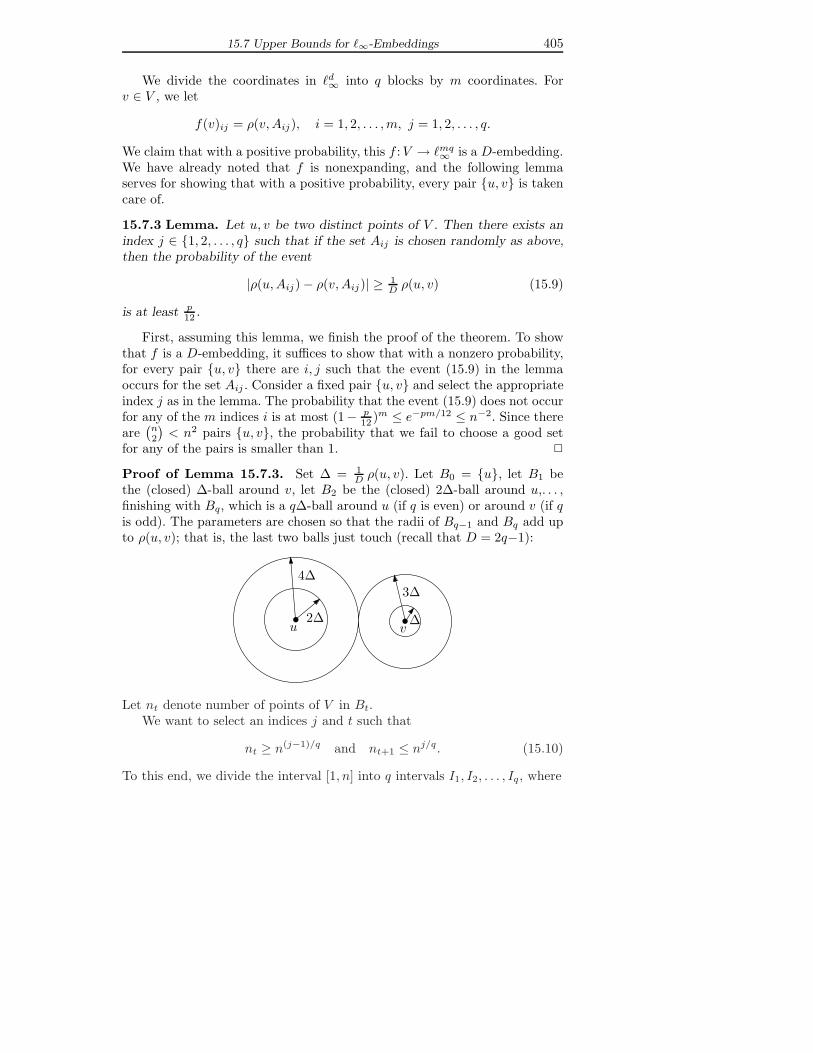
15.7 Upper Bounds for "!-Embeddings 405

We divide the coordinates in #d" into q blocks by m coordinates. Forv % V , we let

f(v)ij = !(v, Aij), i = 1, 2, . . . , m, j = 1, 2, . . . , q.

We claim that with a positive probability, this f : V " #mq" is a D-embedding.

We have already noted that f is nonexpanding, and the following lemmaserves for showing that with a positive probability, every pair {u, v} is takencare of.

15.7.3 Lemma. Let u, v be two distinct points of V . Then there exists anindex j % {1, 2, . . . , q} such that if the set Aij is chosen randomly as above,then the probability of the event

|!(u, Aij) * !(v, Aij)| $ 1D !(u, v) (15.9)

is at least p12 .

First, assuming this lemma, we finish the proof of the theorem. To showthat f is a D-embedding, it su!ces to show that with a nonzero probability,for every pair {u, v} there are i, j such that the event (15.9) in the lemmaoccurs for the set Aij . Consider a fixed pair {u, v} and select the appropriateindex j as in the lemma. The probability that the event (15.9) does not occurfor any of the m indices i is at most (1* p

12 )m & e!pm/12 & n!2. Since thereare

!n2

"< n2 pairs {u, v}, the probability that we fail to choose a good set

for any of the pairs is smaller than 1. !

Proof of Lemma 15.7.3. Set % = 1D !(u, v). Let B0 = {u}, let B1 be

the (closed) %-ball around v, let B2 be the (closed) 2%-ball around u,. . . ,finishing with Bq, which is a q%-ball around u (if q is even) or around v (if qis odd). The parameters are chosen so that the radii of Bq!1 and Bq add upto !(u, v); that is, the last two balls just touch (recall that D = 2q*1):

u v%

3%

2%

4%

Let nt denote number of points of V in Bt.We want to select an indices j and t such that

nt $ n(j!1)/q and nt+1 & nj/q. (15.10)

To this end, we divide the interval [1, n] into q intervals I1, I2, . . . , Iq, where


Ij =7n(j!1)/q, nj/q

8.

If the sequence (n1, n2, . . . , nq) is not monotone increasing, i.e., if nt+1 < nt

for some t, then (15.10) holds for the j such that Ij contains nt. On the otherhand, if 1 = n0 & n1 & . . . & nq & n, then by the pigeonhole principle,there exist t and j such that the interval Ij contains both nt and nt+1. Then(15.10) holds for this j and t as well.

In this way, we have selected the index j whose existence is claimed in thelemma, and the corresponding index t. We will show that with probability atleast p

12 , the set Aij , randomly selected with point probability pj , includes apoint of Bt (event E1) and is disjoint from the interior of Bt+1 (event E2);such an Aij satisfies (15.9). Since Bt and the interior of Bt+1 are disjoint,the events E1 and E2 are independent.

We calculate

Prob[E1] = 1 * Prob[Aij 7 Bt = 8] = 1 * (1 * pj)nt $ 1 * e!pjnt .

Using (15.10), we have pjnt $ pjn(j!1)/q = pjp!j+1 = min(12 , pj)p!j+1 $

min(12 , p). For p $ 1

2 , we get Prob[E1] $ 1 * e!1/2 > 13 $ p

3 , while forp < 1

2 , we have Prob[E1] $ 1 * e!p, and a bit of calculus verifies that thelast expression is well above p

3 for all p % [0, 12 ).

Further,

Prob[E2] $ (1 * pj)nt+1 $ (1 * pj)nj/q

$ (1 * pj)1/pj $ 14

(since pj & 12 ). Thus Prob[E1 7 E2] $ p

12 , which proves the lemma. !

Bibliography and remarks. The embedding method discussedin this section was found by Bourgain [Bou85], who used it to proveTheorem 15.8.1 explained in the subsequent section. Theorem 15.7.2is from [Mat96b].

Exercises

1. (a) Find an isometric embedding of #d1 into #2d

". 3

(b) Explain how an embedding as in (a) can be used to compute thediameter of an n-point set in #d1 in time O(d2dn). 3

2. Show that if the unit ball K of some finite-dimensional normed spaceis a convex polytope with 2m facets, then that normed space embedsisometrically into #m". 2

(Using results on approximation of convex bodies by polytopes, this yieldsuseful approximate embeddings of arbitrary norms into #k".)

3. Deduce from Theorem 15.7.2 that every n-point metric space can be D-embedded into #k2 with D = O(log2 n) and k = O(log2 n). 2

15.8 Upper Bounds for Euclidean Embeddings 407

15.8 Upper Bounds for Euclidean Embeddings

By a method similar to the one shown in the previous section, one can alsoprove a tight upper bound on Euclidean embeddings; the method was actuallyinvented for this problem.

15.8.1 Theorem (Bourgain’s embedding into !2). Every n-point metricspace (V, !) can be embedded into a Euclidean space with distortion at mostO(log n).

The overall strategy of the embedding is similar to the embedding into #d"in the proof of Theorem 15.7.2. The coordinates in #d2 are given by distancesto suitable subsets. The situation is slightly more complicated than before:For embedding into #d", it was enough to exhibit one coordinate “taking care”of each pair, whereas for the Euclidean embedding, many of the coordinateswill contribute significantly to every pair. Here is the appropriate analogueof Lemma 15.7.3.

15.8.2 Lemma. Let u, v % V be two distinct points. Then there exist realnumbers %1,%2, . . . ,%q $ 0 with %1 + · · · + %q = 1

4 !(u, v), where q =0log2 n1+1, and such that the following holds for each j = 1, 2, . . . , q: IfAj / V is a randomly chosen subset of V , with each point of V included inAj independently with probability 2!j , then the probability Pj of the event

|!(u, Aj) * !(v, Aj)| $ %j

satisfies Pj $ 112 .

Proof. We fix u and v, and we set rq = 14 !(u, v). For j = 0, 1, . . . , q * 1 we

let r/j be the smallest radius such that both |B(u, r/j )| $ 2j and |B(v, r/j )| $ 2j

where, as usual, B(x, r) = {y % V : !(x, y) & r}, and we set rj = min(r/j , rq).We are going to show that the claim of the lemma holds with %j = rj *rj!1.

We may assume that rj!1 < rq, for otherwise, we have %j = 0 and theclaim holds automatically. We note that rj!1 < rq implies that both of theballs B(u, rj!1) and B(v, rj!1) have at least 2j!1 points.

So let us fix j % {1, 2, . . . , q} with rj!1 < rq, and let Aj / V be a randomsample with point probability 2!j. By the definition of rj , |B0(u, rj)| < 2j

or |B0(v, rj)| < 2j , where B0(x, r) = {y % V : !(x, y) < r} denotes the openball (this holds for j = q, too, because |V | & 2q). We choose the notation u, vso that |B0(u, rj)| < 2j . A random set Aj is good if it intersects B(v, rj!1)and misses B0(u, rj). The former set has cardinality at least 2j!1 (as wasnoted above) and the latter at most 2j. The calculation of the probabilitythat Aj has these properties is identical to the calculation in the proof ofLemma 15.7.3 with p = 1

2 . !

In the subsequent proof of Theorem 15.8.1 we will construct the embed-ding in a slightly roundabout way, which sheds some light on what is really


going on. Define a line pseudometric on V to be any pseudometric + inducedby a mapping ): V " R, that is, given by +(u, v) = |)(u) * )(v)|. Foreach A / V , let +A be the line pseudometric corresponding to the mappingv +" !(v, A). As we have noted, each +A is dominated by !, i.e., +A & !(the inequality between two (pseudo)metrics on the same point set meansinequality for each pair of points).

The following easy lemma shows that if a metric ! on V can be approx-imated by a convex combination of line pseudometrics, each of them domi-nated by !, then a good embedding of (V, !) into #2 exists.

15.8.3 Lemma. Let (V, !) be a finite metric space, and let +1, . . . , +N beline pseudometrics on V with +i & ! for all i and such that

N$

i=1

(i+i $ 1D!

for some nonnegative (1, . . . ,(N summing up to 1. Then (V, !) can be D-embedded into #N2 .

Proof. Let )i: V " R be a mapping inducing the line pseudometric +i. Wedefine the embedding f : V " #N2 by

f(v)i =.(i · )i(v).

Then, on the one hand,

'f(u) * f(v)'2 =N$

i=1

(i+i(u, v)2 & !(u, v)2,

because all +i are dominated by ! and'(i = 1. On the other hand,

'f(u) * f(v)' =# N$

i=1

(i+i(u, v)2%1/2

=# N$

i=1

(i

%1/2# N$

i=1

(i+i(u, v)2%1/2

$N$

i=1

(i+i(u, v)

by Cauchy–Schwarz, and the latter expression is at least 1D !(u, v) by the

assumption. !

Proof of Theorem 15.8.1. As was remarked above, each of the line pseu-dometrics +A corresponding to the mapping v +" !(v, A) is dominated by !.It remains to observe that Lemma 15.8.2 provides a convex combination ofthese line pseudometrics that is bounded from below by 1

48q ·!. The coe!cient


of each +A in this convex combination is given by the probability of A appear-ing as one of the sets Aj in Lemma 15.8.2. More precisely, write .j(A) forthe probability that a random subset of V , with points picked independentlywith probability 2!j , equals A. Then the claim of Lemma 15.8.2 implies, forevery pair {u, v}, $

A+V

.j(A) · +A(u, v) $ 112 %j .

Summing over j = 1, 2, . . . , q, we have

$

A+V

# q$

j=1

.j(A)%· +A(u, v) $ 1

12 ·q$

j=1

%j = 148 !(u, v).

Dividing by q and using'

A+V .j(A) = 1, we arrive at

$

A+V

(A+A $ 148q

!,$

A+V

(A = 1,

with (A = 1q

'qj=1 .j(A). Lemma 15.8.3 now gives embeddability into #2

with distortion at most 48q. Theorem 15.8.1 is proved. !

Remarks. Almost the same proof with a slight modification of Lemma 15.8.3shows that for each p % [1,#), every n-point metric space can be embeddedinto #p with distortion O(log n); see Exercise 1.

The proof as stated produces an embedding into space of dimension 2n,since there are 2n subsets A / V , each of them yielding one coordinate.To reduce the dimension, one can argue that not all the sets A are needed:by suitable Cherno"-type estimates, it follows that it is su!cient to chooseO(log n) random sets with point probability 2!j, i.e., O(log2 n) sets altogether(Exercise 2). Of course, for Euclidean embeddings, an even better dimensionO(log n) is obtained using the Johnson–Lindenstrauss flattening lemma, butfor other #p, no flattening lemma is available.

An algorithmic application: approximating the sparsest cut. Weknow that every n-point metric space can be O(log n)-embedded into #d1 withd = O(log2 n). By inspecting the proof, it is not di!cult to give a randomizedalgorithm that computes such an embedding in polynomial expected time.We show a neat algorithmic application to a graph-theoretic problem.

Let G = (V, E) be a graph. A cut in G is a partition of V into twononempty subsets A and B = V \A. The density of the cut (A, B) is e(A,B)

|A|·|B| ,where e(A, B) is the number of edges connecting A and B. Given G, wewould like to find a cut of the smallest possible density. This problem is NP-hard, and here we discuss an e!cient algorithm for finding an approximateanswer: a cut whose density is at most O(log n) times larger than the densityof the sparsest cut, where n = |V | (the best known approximation guaranteefor a polynomial-time algorithm is better, currently O(

.log n )). Note that


this also allows us to approximate the edge expansion of G (discussed inSection 15.5) within a multiplicative factor of O(log n).

First we reformulate the problem equivalently using cut pseudometrics. Acut pseudometric on V is a pseudometric , corresponding to some cut (A, B),with ,(u, v) = ,(v, u) = 1 for u % A and v % B and ,(u, v) = 0 for u, v % A oru, v % B. In other words, a cut pseudometric is a line pseudometric inducedby a mapping -: V " {0, 1} (excluding the trivial case where all of V getsmapped to the same point). Letting F =

!V2

", the density of the cut (A, B)

can be written as ,(E)/,(F ), where , is the corresponding cut pseudometricand ,(E) =

'{u,v})E ,(u, v). Therefore, we would like to minimize the ratio

R1(,) = ,(E)/,(F ) over all cut pseudometrics , .In the first step of the algorithm we relax the problem, and we find a pseu-

dometric, not necessarily a cut one, minimizing the ratio R1(!) = !(E)/!(F ).This can be done e!ciently by linear programming. The minimized functionlooks nonlinear, but we can get around this by a simple trick: We postulatethe additional condition !(F ) = 1 and minimize the linear function !(E). Thevariables in the linear program are the

!n2

"numbers !(u, v) for {u, v} % F ,

and the constraints are !(u, v) $ 0 (for all u, v), !(F ) = 1, and those express-ing the triangle inequalities for all triples u, v, w % V .

Having computed a !0 minimizing R1(!), we find a D-embedding f of(V, !0) into some #d1 with D = O(log n). If "0 is the pseudometric induced onV by this f , we clearly have R1("0) & D·R1(!0). Now since "0 is an #1-pseudo-metric, it can be expressed as a nonnegative linear combination of suitablecut pseudometrics (Exercise 15.5.3): "0 =

'Ni=1 (i,i, (1, . . . ,(N > 0, N &

d(n*1). It is not di!cult to check that R1("0) $ min{R1(,i): i = 1, 2, . . . , N}(Exercise 3). Therefore, at least one of the ,i is a cut pseudometric satisfyingR1(,i) & R1("0) & D · R1(!0) & D · R1(,0), where ,0 is a cut pseudometricwith the smallest possible R1(,0). Therefore, the cut corresponding to this ,ihas density at most O(log n) times larger than the sparsest possible cut.

Bibliography and remarks. Theorem 15.8.1 is due to Bour-gain [Bou85]. The algorithmic application to approximating the spars-est cut uses the idea of an algorithm for a somewhat more compli-cated problem (multicommodity flow) found by Linial et al. [LLR95]and independently by Aumann and Rabani [AR98]. The improvedO(

.log n ) approximation is due to Arora, Rao, and Vazirani [ARV04].

We will briefly discuss further results proved by variations of Bour-gain’s embedding technique. Many of them have been obtained in thestudy of approximation algorithms and imply strong algorithmic re-sults.Tree metrics. Let G be a class of graphs and consider a graph G % G.Each positive weight function w: E(G) " (0,#) defines a metric onV (G), namely the shortest-path metric, where the length of a pathis the sum of the weights of its edges. All subspaces of the resultingmetric spaces are referred to as G-metrics. A tree metric is a T -metric


for T the class of all trees. Tree metrics generally behave much betterthan arbitrary metrics, but for embedding problems they are far fromtrivial.

Bourgain [Bou86] proved, using martingales, a surprising lowerbound for embedding tree metrics into #2: A tree metric on n pointsrequires distortion #(

.log log n ) in the worst case. His example is the

complete binary tree with unit edge lengths, and for that example,he also constructed an embedding with O(

.log log n ) distortion. For

embedding the complete binary tree into #p, p > 1, the distortion is#((log log n)min(1/2,1/p)), with the constant of proportionality depend-ing on p and tending to 0 as p " 1. (For Banach-space specialists, wealso remark that all tree metrics can be embedded into a given Banachspace Z with bounded distortion if and only if Z is not superreflexive.)In Matousek [Mat99b] it was shown that the complete binary tree isessentially the worst example; that is, every n-point tree metric can beembedded into #p with distortion O((log log n)min(1/2,1/p)). An alter-native, elementary proof was given for the matching lower bound (seeExercise 5 for a weaker version). Another proof of the lower bound,very short but applying only for embeddings into #2, was found byLinial and Saks [LS03] (Exercise 6).

In the notes to Section 15.3 we mentioned that general n-pointmetric spaces require worst-case distortion #(n1/$(d+1)/2%) for embed-ding into #d2, d $ 2 fixed. Gupta [Gup00] proved that for n-point treemetrics, O(n1/(d!1))-embeddings into #d2 are possible. The best knownlower bound is #(n1/d), from a straightforward volume argument. Ba-bilon, Matousek, Maxova, and Valtr [BMMV02] showed that everyn-vertex tree with unit-length edges can be O(

.n )-embedded into #22.

Planar-graph metrics and metrics with excluded minor. A planar-graph metric is a P-metric with P standing for the class of all pla-nar graphs (the shorter but potentially confusing term planar met-ric is used in the literature). Rao [Rao99] proved that every n-pointplanar-graph metric can be embedded into #2 with distortion onlyO(

.log n ), as opposed to log n for general metrics. More generally,

the same method shows that whenever H is a fixed graph and Excl(H)is the class of all graphs not containing H as a minor, then Excl(H)-metrics can be O(

.log n )-embedded into #2. For a matching lower

bound, valid already for the class Excl(K4) (series-parallel graphs),and consequently for planar-graph metrics, see Exercise 15.4.2 or Ex-ercise 15.9.1.

We outline Rao’s method of embedding. We begin with graphswhere all edges have unit weight (this is the setting in [Rao99], butour presentation di"ers in some details), and then we indicate howgraphs with arbitrary edge weights can be treated. The main newingredient in Rao’s method, compared to Bourgain’s approach, is a


result of Klein, Plotkin, and Rao [KPR93] about a decomposition ofgraphs with an excluded minor into pieces of low diameter. Here is thedecomposition procedure.

Let G be a graph, let ! be the corresponding graph metric (with alledges having unit length), and let % be an integer parameter. We fix avertex v0 % V (G) arbitrarily, we choose an integer r % {0, 1, . . . ,%*1}uniformly at random, and we let B1 = {v % V (G): !(v, v0) 4r (mod%)}. By deleting the vertices of B1 from G, the remainingvertices are partitioned into connected components; this is the firstlevel of the decomposition. For each of these components of G \ B1,we repeat the same procedure; % remains unchanged and r is chosenanew at random (but we can use the same r for all the components).Let B2 be the set of vertices deleted from G in this second round,taken together for all the components. The second level of the decom-position consists of the connected components of G \ (B1 6 B2), anddecompositions of levels 3, 4, . . . can be produced similarly. The fol-lowing schematic drawing illustrates the two-level decomposition; thegraph is marked as the gray area, and the vertices of B1 and B2 areindicated by the solid and dashed arcs, respectively.

For planar graphs, it su!ces to use a 3-level decomposition, and forevery fixed graph H , there is a suitable k = k(H) such that a k-leveldecomposition is appropriate for all graphs G % Excl(H).

Let B = B1 6 · · · 6 Bk; this can be viewed as the boundary of thecomponents in the k-level decomposition. Here are the key propertiesof the decomposition:

(i) For each vertex v % V (G), we have !(v, B) $ c1% with proba-bility at least c2, for suitable constants c1, c2 > 0. The probability iswith respect to the random choices of the parameters r at each levelof the decomposition. (This is not hard to see; for example, in thefirst level of the decomposition, for every fixed v, !(v, v0) is some fixednumber and it has a good chance to be at least c1% away, modulo %,from a random r.)


(ii) Each component in the resulting decomposition has diameterat most O(%). (This is not so easy to prove, and it is where one needsk = k(H) su!ciently large. For H = K3,3, which includes the case ofplanar graphs, the proof is a relatively simple case analysis.)

Next, we describe the embedding of V (G) into #2 in several steps.First we consider % and the decomposition as above fixed, and we letC1, . . . , Cm be the components of G \ B. For all the Ci, we chooserandom signs "(Ci) % {*1, +1} uniformly and independently. For avertex x % V (G), we define "(x) = 0 if x % B and "(x) = "(Ci)if x % V (Ci). Then we define the mapping )B,%: V (G) " R by)B,%(v) = "(x) · !(x, B) (the distance of x to the boundary signed bythe component’s sign). This )B,% induces a line pseudometric +B,%,and it is easy to see that +B,% is dominated by !.

Let C be a constant such that all the Ci have diameter at mostC%, and let x, y % V (G) be such that C% < !(x, y) & 2C%. Suchx and y certainly lie in distinct components, and "(x) (= "(y) withprobability 1

2 . With probability at least c2, we have !(x, B) $ c1%,and so with a fixed positive probability, +B,% places x and y at distanceat least c1%.

Now, we still keep % fixed and consider +B,% for all possible B and". Letting (B,% be the probability that a particular pair (B,") resultsfrom the decomposition procedure, we have

$

B,%

(B,%+B,%(x, y) = #(!(x, y))

whenever C% < !(x, y) & 2C%. As in the proof of Lemma 15.8.3,this yields a 1-Lipschitz embedding f": V (G) " #N2 (for some N) thatshortens distances for pairs x, y as above by at most a constant factor.(It is not really necessary to use all the possible pairs (B,") in theembedding; it is easy to show that const · log n independent randomB and " will do.)

To construct the final embedding f : V (G) " #2, we let f(v) be theconcatenation of the vectors f" for % % {2j: 1 & 2j & diam(G)}. Nodistance is expanded by more than O(

.log diam(G) ) = O(

.log n ),

and the contraction is at most by a constant factor, and so we havean embedding into #2 with distortion O(

.log n ).

Why do we get a better bound than for Bourgain’s embedding?In both cases we have about log n groups of coordinates in the em-bedding. In Rao’s embedding we know that for every pair (x, y), oneof the groups contributes at least a fixed fraction of !(x, y) (and nogroup contributes more than !(x, y)). Thus, the sum of squares of thecontributions is between !(x, y)2 and !(x, y)2 log n. In Bourgain’s em-bedding (with a comparable scaling) no group contributes more than!(x, y), and the sum of the contributions of all groups is at least a


fixed fraction of !(x, y). But since we do not know how the contri-butions are distributed among the groups, we can conclude only thatthe sum of squares of the contributions is between !(x, y)2/ logn and!(x, y)2 log n.

It remains to sketch the modifications of Rao’s embedding for agraph G with arbitrary nonnegative weights on edges. For the un-weighted case, we defined B1 as the vertices lying exactly at the givendistances from v0. In the weighted case, there need not be verticesexactly at these distances, but we can add artificial vertices by subdi-viding the appropriate edges; this is a minor technical issue. A moreserious problem is that the distances !(x, y) can be in a very widerange, not just from 1 to n. We let % run through all the relevantpowers of 2 (that is, such that C% < !(x, y) & 2C% for some x (= y),but for producing the decomposition for a particular %, we use a mod-ified graph G" obtained from G by contracting all edges shorter than"2n . In this way, we can have many more than log n values of %, butonly O(log n) of them are relevant for each pair (x, y), and the analysisworks as before.

Gupta, Newman, Rabinovich, and Sinclair [GNRS99] conjecturedthat for any fixed graph H , Excl(H)-metrics might be O(1)-em-beddable into #1 (the constant depending on H). They proved the con-jecture for H = K4 and for H = K2,3 (outerplanar graphs). Chekuri,Gupta, Newman, Rabinovich, and Sinclair [CGN+03] established theconjecture for k-outerplanar graphs (for every fixed k), which are,roughly speaking, graphs admitting a planar drawing with no k+1disjoint properly nested cycles, a canonical example being the k!ngrid.Volume-respecting embeddings. Feige [Fei00] introduced an interest-ing strengthening of the notion of the distortion of an embedding,concerning embeddings into Euclidean spaces. Let f : (V, !) " #2 bean embedding that for simplicity we require to be 1-Lipschitz (nonex-panding). The usual distortion of f is determined by looking at pairsof points, while Feige’s notion takes into account all k-tuples for somek $ 2. For example, if V has 3 points, every two with distance 1, thenthe following two embeddings into #22 have about the same distortion:

But while the left embedding is good in Feige’s sense for k = 3, theright one is completely unsatisfactory. For a k-point set P ) #2, de-fine Evol(P ) as the (k*1)-dimensional volume of the simplex spannedby P (so Evol(P ) = 0 if P is a!nely dependent). For a k-pointmetric space (S, !), the volume Vol(S) is defined as supf Evol(f(S)),where the supremum is over all 1-Lipschitz f : S " #2. An embedding


f : (V, !) " #2 is (k, D) volume-respecting if for every k-point subsetS / V , we have D · Evol(f(S))1/(k!1) $ Vol(S)1/(k!1). For D small,this means that the image of any k-tuple spans nearly as large a vol-ume as it possibly can for a 1-Lipschitz map. (Note, for example, thatan isometric embedding of a path into #2 is not volume-respecting.)

Feige showed that Vol(S) can be approximated quite well byan intrinsic parameter of the metric space (not referring to embed-dings), namely, by the tree volume Tvol(S), which equals the prod-ucts of the edge lengths in a minimum spanning tree on S (withrespect to the metric on S). Namely, Vol(S) & 1

(k!1)! Tvol(S) &2(k!2)/2 Vol(S). He proved that for any n-point metric space andall k $ 2, the embedding as in the proof of Theorem 15.8.1 is(k, O(log n +

.k log n log k )) volume-respecting. Later Krauthgamer,

Lee, Mendel, and Naor [KLMN04] established the existence of embed-dings that are (k, O(log n)) volume-respecting for all k = 1, 2, . . . , n,which is optimal.

The notion of volume-respecting embeddings currently still lookssomewhat mysterious. In an attempt to convey some feeling aboutit, we outline Feige’s application and indicate the use of the volume-respecting condition in it. He considered the problem of approximat-ing the bandwidth of a given n-vertex graph G. The bandwidth isthe minimum, over all bijective maps ): V (G) " {1, 2, . . . , n}, ofmax{|)(u) * )(v)|: {u, v} % E(G)} (so it has the flavor of an approx-imate embedding problem). Computing the bandwidth is NP-hard,but Feige’s ingenious algorithm approximates it within a factor ofO((log n)const). The algorithm has two main steps: First, embed thegraph (as a metric space) into #m2 , with m being some suitable powerof log n, by a (k, D) volume-respecting embedding f , where k = log nand D is as small as one can get. Second, let * be a random line in#m2 and let -(v) denote the orthogonal projection of f(v) on *. This-: V (G) " * is almost surely injective, and so it provides a linear or-dering of the vertices, that is, a bijective map ): V (G) " {1, 2, . . . , n},and this is used for estimating the bandwidth.

To indicate the analysis, we need the notion of local density of thegraph G: ld(G) = max{|B(v, r)|/r: v % V (G), r = 1, 2, . . . , n}, whereB(v, r) are all vertices at distance at most r from v. It is not hard tosee that ld(G) is a lower bound for the bandwidth, and Feige’s analysisshows that O(ld(G)(log n)const) is an upper bound.

One first verifies that with high probability, if {u, v} % E(G), thenthe images -(u) and -(v) on * are close; concretely, |-(u) * -(v)| &% = O(

.(log n)/m ). For proving this, it su!ces to know that f is

1-Lipschitz, and it is an immediate consequence of measure concentra-tion on the sphere. If b is the bandwidth obtained from the orderinggiven by -, then some interval of length % on * contains the images of


b vertices. Call a k-tuple S ) V (G) squeezed if -(S) lies in an intervalof length %. If b is large, then there are many squeezed S. On theother hand, one proves that, not surprisingly, if ld(G) is small, thenVol(S) is large for all but a few k-tuples S ) V (G). Now, the volume-respecting condition enters: If Vol(S) is large, then conv(f(S)) haslarge (k*1)-dimensional volume. It turns out that the projection of aconvex set in #m2 with large (k*1)-dimensional volume on a randomline is unlikely to be short, and so S with large Vol(S) is unlikely to besqueezed. Thus, by estimating the number of squeezed k-tuples in twoways, one gets an inequality bounding b from above in terms of ld(G).

Vempala [Vem98] applied volume-respecting embeddings in an-other algorithmic problem, this time concerning arrangement of graphvertices in the plane. Moreover, he also gave alternative proof of someof Feige’s lemmas. Rao in the already mentioned paper [Rao99] alsoobtained improved volume-respecting embeddings for planar metrics. 9 NEW 9Probabilistic approximation by dominating trees. As we have seen, inBourgain’s method, for a given metric ! one constructs a convex com-bination

'(i+i $ 1

D !, where +i are line pseudometrics dominatedby !. An interesting “dual” result is the possibility of approximatingevery ! by a convex combination

'Ni=1 (i,i, where this time the in-

equalities go in the opposite direction: ,i $ ! and'(i,i & D!, with

D = O(log n). The ,i are not line metrics (and in general they cannotbe), but they are tree metrics. (It is important to use many trees, sinceit is impossible to approximate a general metric by a single tree metricwith any reasonable distortion—consider the shortest-path metric ofa cycle of length n.) Since tree metrics embed isometrically into #1,the result yields an alternative proof of O(log n)–embeddability of alln-point metric spaces into #1. This also implies that we must haveD = #(log n) in the above result.

The approximation of ! by tree metrics as above is usually called aprobabilistic approximation by dominating trees, which refers to the fol-lowing alternative view. The coe!cients (1, . . . ,(N and the tree met-rics ,1, . . . , ,N specify a probability distribution on tree metrics, where,i is chosen with probability (i. Then the condition

'(i,i & D!

translates as follows: If we pick a tree metric , at random accordingto this distribution, then E[,(x, y)] & D!(x, y) for every x, y (and,(x, y) $ !(x, y) always by the condition ,i $ !). This is convenientlyused in approximation algorithms: If we want to solve some optimiza-tion problem for a given metric !, we can compute the ,i and (i andsolve the problem for the random tree metric , , which is usually mucheasier than solving it for a general metric. Often it can be shown thatthe expected value of the optimal solution for , is not very far fromthe optimal value for the original metric !.


The first result about probabilistic approximation by dominat-ing trees, with D = 2O(

.log n log log n ), is due to Alon, Karp, Peleg,

and West [AKPW95]. A fundamental progress was made by Bartal[Bar96], who obtained D = O(log2 n) (improved to O(log n log log n)in a later paper), and documented the significance of the result bymany impressive applications. This line of research was crowned byFakcharoenphol, Talwar, and Rao [FRT03], who obtained the optimalbound D = O(log n), with a clean few-page proof.

The construction of Alon et al. [AKPW95] assumes that the in-put metric is given as the shortest-path metric of a graph G (withweighted edges), and the resulting tree metrics ,i are induced by span-ning trees of G. The subsequent constructions [Bar96], [FRT03] don’tshare this property, but Elkin, Emek, Spielman, and Teng [EEST05]later achieved D = O((log n log log n)2) using spanning trees.

Bartal [Bar96] also introduced the useful notion of a k-hierarchicallywell-separated tree metric, where k $ 1 is a real parameter. Here wepresent a newer, and apparently more convenient, definition by Bar-tal, Bollobas, and Mendel [BBM01]. A 1-hierarchically well-separatedtree metric is the same as an ultrametric, that is, a metric that can berepresented as the shortest-path metric on the leaves of a rooted treeT (with weighted edges) such that all leaves have the same distancefrom the root. For k > 1, we moreover require that h(v) & h(u)/kwhenever v is a child of u in T , where h(v) denotes the distance of vto the nearest leaves. In the result of [FRT03] cited above, one can getthe ,i k-hierarchically well-separated for every prescribed k $ 1, withthe constant in the bound D = O(log n) depending on k (the sameholds for Bartal’s earlier results).

We sketch the construction of Fakcharoenphol et al. [FRT03]. Wemay suppose that the given n-point metric space (V, !) has all dis-tances between 1 and 2m. We describe a randomized algorithm forgenerating a random tree metric , with , $ ! always and E[,(x, y)] &O(log n·!(x, y)) for every x, y. The (i and ,i specifying the probabilitydistribution are thus given implicitly (and actually, the procedure asdescribed may output infinitely many distinct ,i, but easy modifica-tions would lead to a finite collection). We first generate a sequence(Pm,Pm!1, . . . ,P0), where each Pi is a partition of V , and Pi refinesPi+1; that is, each set in Pi+1 is a disjoint union of some sets of Pi.We begin with Pm = {V }, and proceed to Pm!1,Pm!2, . . . , finishingwith P0 that consists of n singleton sets. The diameter of each set inPi is at most 2i+1. Having constructed these Pi, we arrange them intoa rooted tree in a natural way. The vertices of the tree have the form(S, i), S % Pi, i = 0, 1, . . . , m. The root is (V, m), and the children of avertex (S, i+1), S % Pi+1, are (T, i) with T % Pi and T / S. The edgeconnecting (S, i+1) to (T, i) has length 2i+1, and finally, the metric ,


is the shortest-path metric induced by this tree on the set of its leaves(the leaves correspond to points of V ). It is easily seen that , $ ! andthat , is 2-hierarchically well-separated.

The construction of the Pi starts with arranging the points of V ina random order (v1, v2, . . . , vn), and choosing a real number & % [1, 2]uniformly at random. Supposing that Pi+1 has already been con-structed, we set &i = &2i!1, and for every S % Pi+1 we generate a par-tition of S into disjoint subsets S1, . . . , Sn (don’t get confused by then; most of the S" are going to be empty!). Namely, for # = 1, 2, . . . , n,we set S" = {v % S \ (S1 6 · · · 6 S"!1): !(v, vi) & &i}. That is, thefirst vertex v1 in the random order, the “king,” comes to S and hecan take all vertices that are closer to him than &i. Then, after theking has been satisfied, the “prime minister” v2 comes, and he is al-lowed to grab from the leftovers all that is in his &i-neighborhood.Then v3 comes, and so on until vn. The partition Pi consists of allnonempty S" thus generated for all S % Pi+1 and all #. The proof ofE[,(x, y)] & O(log n · !(x, y)) is a simple but ingenious probabilisticanalysis, for which we refer to [FRT03]. : NEW :

Exercises

1. (Embedding into #p) Prove that under the assumptions of Lemma 15.8.3,the metric space (V, !) can be D-embedded into #Np , 1 & p & #, withdistortion at most D. (You may want to start with the rather easy casesp = 1 and p = #, and use Holder’s inequality for an arbitrary p.) 3

2. (Dimension reduction for the embedding)(a) Let E1, . . . , Em be independent events, each of them having proba-bility at least 1

12 . Prove that the probability of no more than m24 of the

Ei occurring is at most e!cm, for a su!ciently small positive constant c.Use suitable Cherno"-type estimates or direct estimates of binomial co-e!cients. 3

(b) Modify the proof of Theorem 15.8.1 as follows: For each j =1, 2, . . . , q, pick sets Aij independently at random, i = 1, 2, . . . , m,where the points are included in Aij with probability 2!j and wherem = C log n for a su!ciently large constant C. Using (a) and Lem-mas 15.8.2 and 15.8.3, prove that with a positive probability, the embed-ding f : V " #qm

2 given by f(v)ij = !(v, Aij) has distortion O(log n). 3

3. Let a1, a2, . . . , an, b1, b2, . . . , bn, (1,(2, . . . ,(n be positive real numbers.Show that

(1a1 + (2a2 + · · · + (nan

(1b1 + (2b2 + · · · + (nbn$ min{a1

b1,a2

b2, . . . ,

an

bn}.

2

4. Let Pn be the metric space {0, 1, . . . , n} with the metric inherited fromR (or a path of length n with the graph metric). Prove the following


Ramsey-type result: For every D > 1 and every $ > 0 there exists ann = n(D, $) such that whenever f : Pn " (Z,") is a D-embedding of Pn

into some metric space, then there are a < b < c, b = a+c2 , such that f

restricted to the subspace {a, b, c} of Pn is a (1+$)-embedding. That is,if a su!ciently long path is D-embedded, then it contains a scaled copyof a path of length 2 embedded with distortion close to 1. 4

Can you extend the proof so that it provides a scaled copy of a path oflength k?

5. (Lower bound for embedding trees into #2)(a) Show that for every $ > 0 there exists % > 0 with the followingproperty. Let x0, x1, x2, x(

2 % #2 be points such that 'x0 * x1', 'x1 *x2', 'x1 * x(

2' % [1, 1 + %] and 'x0 * x2', 'x0 * x(2' % [2, 2 + %] (so all the

distances are almost like the graph distances in the following tree, exceptpossibly for the one marked by a dotted line).

x1x0

x2

x(2

Then 'x2 * x(2' & $; that is, the remaining distance must be very short.

3

(b) Let Tk,m denote the complete k-ary tree of height m; the followingpicture shows T3,2:

root

Show that for every r and m there exists k such that whenever the leavesof Tk,m are colored by r colors, there is a subtree of Tk,m isomorphic toT2,m with all leaves having the same color. 2

(c) Use (a), (b), and Exercise 4 to prove that for any D > 1 there existm and k such that the tree Tk,m considered as a metric space with theshortest-path metric cannot be D-embedded into #2. 4

6. (Another lower bound for embedding trees into #2)(a) Let x0, x1, . . . , xn be arbitrary points in a Euclidean space (we thinkof them as images of the vertices of a path of length n under some em-bedding). Let ' = {(a, a+2k, a+2k+1): a = 0, 1, 2, . . . , a+2k+1 & n, k =0, 1, 2 . . .}. Prove that

$

(a,b,c))#

'xa * 2xb + xc'2

(c * a)2&

n!1$

a=0

'xa * xa+1'2;

this shows that an average triple (xa, xb, xc) is “straight” (and providesan alternative solution to Exercise 4 for Z = #2). 3


(b) Prove that the complete binary tree T2,m requires #(.

log m ) dis-tortion for embedding into #2. Consider a nonexpanding embeddingf : V (T2,m) " #2 and sum the inequalities as in (a) over all images ofthe root-to-leaf paths. 4

7. (Bourgain’s embedding of complete binary trees into #2) Let Bm = T2,m

be the complete binary tree of height m (notation as in Exercise 5).We identify the vertices of Bm with words of length at most m overthe alphabet {0, 1}: The root of Bm is the empty word, and the sonsof a vertex w are the vertices w0 and w1. We define the embeddingf : V (Bm) " #|V (Bm)|!1

2 , where the coordinates in the range of f areindexed by the vertices of Bm distinct from the root, i.e., by nonemptywords. For a word w % V (Bm) of length a, let f(w)u =

.a*b+1 if u is

a nonempty initial segment of w of length b, and f(w)u = 0 otherwise.Prove that this embedding has distortion O(

.log m ). 4

8. Prove that any finite tree metric can be isometrically embedded into #1.3

9. (Low-dimensional embedding of trees)(a) Let T be a tree (in the graph-theoretic sense) on n $ 3 vertices. Provethat there exist subtrees T1 and T2 of T that share a single vertex andno edge and together cover T , such that max(|V (T1)|, |V (T2)|) & 1+2

3n.3

(b) Using (a), prove that every tree metric space with n points can beisometrically embedded into #d" with d = O(log n). 4

This result is from [LLR95].

15.9 Approximate Embeddings 2002–20059 NEW 9

The progress in the field considered in the present chapter has been amazingsince the first edition of the book. Mainly by the e"orts of several young re-searchers, many problem that were open and considered di!cult in 2002 havebeen solved in the next few years. The development is vividly documentedin the problem collection [Mat05], which started at a workshop in 2002 andhas been continuously updated with new problems and solutions.

Few of the new results are mentioned in updated remarks to the previoussections or in the newly written Section 15.6. Here we outline some more, ina format similar to the bibliographic parts of the other sections.

Starring: !1 metrics. Most of the main results from the period 2002–2005have a unifying theme: a key role of #1. There are several sources of its promi-nence. First, from a mathematical point of view, #1 can be thought of as a“frontier of wilderness.” The Euclidean metrics have all kinds of nice proper-ties, and #p with 1 < p < # share some of them, such as uniform convexity.On the other side, #" metrics are the same as all metrics, and so nobody ex-pects anything nice from them. The space #1 is somewhere in between, with a

15.9 Approximate Embeddings 2002–2005 421

(deceptively) simple definition of the norm, some good properties, but manysurprises and mysteries. For example, the following famous innocent-lookingproblem is still open: Does the 3-dimensional space #31 have a finite order ofcongruence? A metric space M is said to have order of congruence at mostm if every finite metric space that is not isometrically embeddable in M hasa subspace with at most m points that is not embeddable in M .

A second source of importance of #1 is algorithmic. As we saw at the endof Section 15.8, low-distortion embeddings into #1 lead to e!cient approxima-tion algorithms for partitioning problems such as the sparsest cut. Moreover,various e!cient data structures are known for #1-metrics, for example, fornearest neighbor queries (see, e.g., Indyk’s survey [Ind04]). So #1 is muchricher than #2 but still manageable in many respects.

No flattening in !1. Given the algorithmic importance of #1 and theusefulness of the Jonhson–Lindenstrauss flattening lemma (Theorem 15.2.1),it was natural to ask for an analogue of the flattening lemma in #1. In abreakthrough paper, Brinkman and Charikar [BC03] showed that flatteningis almost impossible. Namely, for all D $ 1, there exist n-point subspaces of#1 that cannot be D-embedded into #d1 unless d = #(nc/D2

), with a positiveabsolute constant c. A di"erent and simpler proof was found by Lee and Naor[LN04]. Both proofs use the same example, the shortest-path metrics of thediamond graphs defined in Exercise 15.4.2. We outline the latter proof, whichis a beautiful application of the geometry of #p spaces with p > 1 in a questionseemingly concerning only p = 1. First, one can check that all diamond graphsembed into #1 (unlimited dimension) with constant distortion. Second, Leeand Naor proved that for every p > 1 any embedding of a diamond graph into#p (unlimited dimension) requires distortion at least #(

.(p*1) log n ), with

the implicit constant independent of p. The proof is based on the followingclassical inequality for #p-spaces: 'x+ y'2

p + (p*1)'x* y'2p & 2('x'2

p + 'y'2p)

for all x, y % #p (this inequality can be traced back to Figiel [Fig76], althoughit is not stated explicitly there). Given the inequality, the proof is not hard,and it proceeds analogously to the proof for p = 2 in Exercise 15.4.2. Third, asimple calculation shows that for p(d) := 1+ 1

log d , the identity map Rd " Rd

is an O(1)-embedding of #d1 into #dp(d), and consequently, a D-embedding ofany space X into #d1 yields an O(D)-embedding of X into #p(d). Hence forthe diamond graphs we obtain D = #(

.1 + (p(d)*1) log n ), and calculation

leads to the claimed lower bound d $ nc/D2.

This bound is known to be almost tight for D of order.

log n log log n,since by a result of Arora, Lee, and Naor [ALN05] discussed later, every n-point subspace of #1 embeds into #2 with distortion O(

.log n log log n), the

image can further be flattened to #O(log n)2 with distortion 2, say, and the

latter space 2-embeds into #O(log n)1 .


In spite of the almost complete answer for #1, the situation concerningflattening in #p for p (% {1, 2,#} is unclear, and in particular, no nontriviallower bound is known for p % (1, 2).

Metrics of negative type and !1. Let V be a finite set. A metric !on V is called of negative type if there is a mapping f : V " #2 such that!(u, v) = 'f(u) * f(v)'2 for all u, v % V . That is, the distances in ! can berepresented as squared Euclidean distances of points in a Euclidean space,or in other words, V with the metric .

! embeds isometrically into #2. Thereis a subtlety in this definition: Not every embedding f : V " #2 induces ametric of negative type, since the distance function given by 'f(u) * f(v)'2

generally need not obey the triangle inequality! Indeed, if f(u), f(v), f(w)are three distinct collinear points, for instance, then the triangle inequality isviolated. In the terminology introduced after Proposition 15.5.2, metrics ofnegative type exactly correspond to points in the intersection of the metriccone with the cone of squared Euclidean metrics.

As was mentioned in the notes to Section 15.5, every #1 metric is also ametric of negative type. On the other hand, not every metric of negative typeembeds isometrically into #1, but it was conjectured by Goemans and inde-pendently by Linial that metrics of negative type are not very far from being#1; namely, that all metrics of negative type embed into #1 with distortionbounded by a universal constant.

To appreciate the importance of this conjecture, let us return to the prob-lem of finding a sparsest cut in a given graph G = (V, E). At the end ofSection 15.8 we have seen that the problem is equivalent to computing an #1metric , on V such that

'u,v)V ,(u, v) = n2 and ,(E) =

'{u,v})E ,(u, v)

is minimum (we have changed the scaling compared to Section 15.8, in or-der to have simpler expressions later on). The minimum is attained by a cutpseudometric that corresponds to a sparsest cut. This latter problem, whichis an instance of linear optimization over the cone of all #1-metrics (usuallycalled the cut cone), is NP-hard, and we want to solve it approximately. Thealgorithm outlined in Section 15.8 minimizes over all metrics, instead of justall #1 metrics, and then it approximates the optimum metric by an #1 met-ric. This is based on two key facts: First, linear optimization over the metriccone can be done e!ciently, and second, a general metric can be O(log n)-embedded in #1. So a natural way to improve on the approximation factor isto take some subclass of all metrics such that, first, linear optimization overit is still “easy,” and second, every metric in this class can be embedded in#1 with distortion o(log n), or even a constant.

Linear optimization over all metrics of negative type can be solved e!-ciently by semidefinite programming, which was briefly discussed at the endof Section 15.5. Indeed, as we have shown there, a function , : V !V " Ris a squared Euclidean (pseudo)metric on V = {1, 2, . . . , n} if and only ifthere exists an n!n symmetric positive semidefinite matrix Q such that,(u, v) = quu + qvv * 2quv for all u, v. In order to pass from squared Eu-


clidean metrics to metrics of negative type, it su!ces to enforce the triangleinequality ,(u, w) & ,(u, v)+ ,(v, w) for all u, v, w % V , which means impos-ing linear inequalities for the entries of Q. Thus, the problem of minimizinga given linear function, such as ,(E), over all metrics of negative type on V ,possibly satisfying additional linear constraints such as

'u,v)V ,(u, v) = n2,

is an instance of semidefinite programming, and it can be solved (reasonably)e!ciently. Hence, if we could embed every metric of negative type into #1 withdistortion at most D, and do so e!ciently, then we could approximate thesparsest cut problem with ratio at most D.

The bad news is that the Goemans–Linial conjecture is false: Khot andVishnoi [KV05] proved that there are n-point metrics of negative type requir-ing distortion #((log log n)1/4!!) for embedding into #1, for every fixed $ > 0.Their proof of this (purely geometric) fact is based on algorithmic thinkingand, in particular, on probabilistically checkable proofs, the current most pow-erful device for establishing hardness of approximation. Technically, it relieson advanced results in harmonic analysis. We will not attempt to sketch theproof, or even the construction of their badly embeddable example. The lowerbound was improved to #(log log n), with the same example, by Krauthgamerand Rabani [KR06].

Improved approximation to sparsest cut. The good news is that one canimprove on the O(log n) approximation factor for the sparsest cut problemby the above approach, although not all the way to a constant. However, thehistorical development went di"erently: First came a breakthrough by Arora,Rao, and Vazirani [ARV04], who discovered an O(

.log n )-approximation al-

gorithm for the sparsest cut, as well as for several other graph-partitioningproblems, and only later and with considerable additional e"ort it was under-stood that the geometric part of their argument also leads to low-distortionembeddings.

Here is a “hyperplane-partitioning” algorithm for the sparsest cut. Givena graph G = (V, E), by semidefinite programming we find a metric , of neg-ative type minimizing ,(E) subject to

'u,v)V ,(u, v) = n2, as was outlined

above. We fix v0 % V such that the ball B(v0, 4) in the , -metric containsthe largest number of points of V ; since the sum of all distances is n2, it iseasily calculated that |B(v0, 4)| $ 3

4n. Next, we let xv, v % V , be points in #n2representing , , i.e. with 'xu * xv'2 = ,(u, v). This geometric representationof , is used to find two large and well-separated subsets L, R ) V . Namely,we choose a random hyperplane h through xv0 , and we let S be the slabconsisting of points with distance at most $/

.n from h, where $ > 0 is a

suitable small constant. We let HL and HR denote the two open half-spaceswhose union is the complement of the slab S, and we define disjoint subsetsL, R / V by L = {v % V : xv % HL} and R = {v % V : xv % HR}. Theseare not yet the final L and R; we have to prune them as follows: As long asthere is a pair (u, v) % L!R with ,(u, v) & C/

.log n, for a suitable constant

C, we remove u from L and v from R. The resulting L and R clearly have


, -distance at least C/.

log n, and they are used as a “core” of the desiredsparse cut. Namely, we sort the vertices of V as (v1, v2, . . . , vn) according totheir , -distance to L, and we output the sparsest among the n*1 “candidate”cuts ({v1, . . . , vi}, {vi+1, . . . , vn}), i = 1, 2, . . . , n*1. Actually, one more ad-justment of the algorithm is needed: At the beginning, if there is an u % Vwith |B(u, 1

4 )| $ n2 , then we skip the choice of the random hyperplane and

use the ball B(u, 14 ) as the set L that defines the candidate cuts.

The described algorithm comes essentially from [ARV04], but the authorsproved only an approximation bound of O((log n)2/3) for it, and they used amore complicated algorithm to get O(

.log n ). Lee [Lee05] showed that the

simpler algorithm above has approximation ratio O(.

log n ) as well.The most time-consuming part of the algorithm is the semidefinite pro-

gramming step. Arora, Hazan, and Kahale [AHK04] found a way of replacingit by an iterative method of Freund and Schapire for solving zero-sum games,and they achieved a near-quadratic running time.

Improved embedding of metrics of negative type. The heart of theingenious and somewhat complicated analysis of algorithm described above isin showing that with probability bounded below by a constant, the resultingsets L and R are large; |L|, |R| = #(n). In particular, it follows that for any n-point V with a metric , of negative type normalized so that

'u,v)V ,(u, v) =

n2, and with no very large and tight cluster (a ball of radius 14 containing at

least half of the set), there are subsets L, R ) V of size #(n) with ,(L, R) =#((log n)!1/2).

To understand the statement better, let us consider the m-dimensionalHamming cube (with n = 2m) as an example; since the average distance init is of order m, we have to scale it by roughly 1

m to meet the condition'u,v)V ,(u, v) = n2. So in the original Hamming cube we look for linear-size

subsets separated by a gap of order.

m. On the one hand, we can take allvertices with at most m

2 ones for L and all vertices with at least m2 +

.m ones

for R. On the other hand, showing that the gap cannot be of order largerthan

.m is a nice exercise using measure concentration (Theorem 14.2.3

slightly generalized to the case of P[A] bounded below by an arbitrary positiveconstant, rather than by 1

2 ). So the result of Arora et al. can be thought of asshowing that, in a sense, no metric space of negative type can have measureconcentration stronger than the Hamming cube.

The result was further refined, analyzed, and applied in subsequent pa-pers. Lee [Lee05] simplified the proof and provided a stronger version (roughlyspeaking, the sets R and L generated by the algorithm are shown to be “morerandom” than in [ARV04], which is crucial for low-distortion embeddings; seebelow). Naor, Rabani, and Sinclair [NRS04] derived a graph-theoretic conse-quence, and observed that the proof of [ARV04] uses only little of the prop-erties of metrics of negative type: They proved analogous results for metricsuniformly embeddable into #2 and for metrics quasisymmetrically embeddableinto #2. (The latter, less well-known notion, due to Beurling and Ahlfors,


is defined as follows: An embedding f : (X, !) " (Y,") is quasisymmetricwith modulus ', where ': [0,#] " [0,#) is a strictly increasing function, if"(f(x), f(y))/"(f(x), f(z)) & '(!(x, y)/!(x, z)) for every x, y, z % X .)

Chawla, Gupta, and Racke [CGR05] used the geometric results of [ARV04]for proving that every metric of negative type on n points embeds into #2with distortion O((log n)3/4), and Arora, Lee, and Naor [ALN05] obtained animproved and nearly tight bound of O(

.log n · log log n). This , of course, also

provides embeddings of negative type metrics into #1, and thus an alternativealgorithm for the sparsest cut problem, whose approximation guarantee islittle worse than that of Arora, Rao, and Vazirani [ARV04], but which is moregeneral: It can also handle a weighted version of the problem (with generalcapacities and demands, for those familiar with multicommodity flows).

Since #1 metrics are a subclass of metrics of negative type, Arora, Lee,and Naor [ALN05] also almost solved another famous open problem: Whatis the largest distortion needed for embedding an n-point #1 metric into #2?By their result we now know that the m-dimensional Hamming cube, whichneeds distortion #(

.m ), is nearly the worst example.

Refined embedding methods. The proof of Arora et al. [ALN05] com-bines the main geometric result of [ARV04] mentioned above with a general-purpose embedding technique, called measured descent. This technique, de-veloped by Krauthgamer, Lee, Mendel, and Naor [KLMN04], is a commongeneralization and significant refinement of the embedding methods of Bour-gain and of Rao, and it has been applied for solving several other problems.We outline some of the key ingredients.

We want to embed an n-point metric space (V, !) into #2 (variations forother target spaces are obviously possible but here we stick to the Euclideancase). We may assume, after re-scaling !, that the distances in (V, !) arebetween 1 and 2m. The first idea for constructing a low-distortion embedding,present explicitly in Rao’s embedding (see the notes to Section 15.8), and lessexplicitly in Bourgain’s embedding, is to divide the task conceptually into twosteps:

(i) For each scale % = 20, 21, . . . , 2m, construct a mapping )": V " #2 that“takes care” of all pairs (u, v) % V !V with % & !(u, v) < 2%.

(ii) Combine the )" over all % into a single D-embedding f : V " #2.

First we need to clarify what do we mean by “taking care” in (i). FollowingLee [Lee05], we say that a mapping ): V " #2 is an embedding with deficiencyD0 at scale % if ) is 1-Lipschitz (nonexpanding) and we have ')(u)*)(v)'2 $!(u, v)/D0 for all u, v % V with % & !(u, v) < 2%.

We have already seen an example in the description of Rao’s embedding:If the reader has the energy to look it up, she can see that the mappingf" constructed there was an embedding with deficiency O(1) at scale C%.A useful abstraction of the approach used there is the notion of padded de-composition. A padded decomposition should be imagined as a randomized


algorithm that receives a finite metric space (V, !) as input and outputs arandom partition P of V . The definition is as follows: A D0-padded decom-position at scale % for (V, !) is a probability distribution on partitions of V ,such that

• In each partition P occurring in this distribution, all classes have diam-eter smaller than %.

• For every v % V , the ball B(v,%/D0) is fully contained in a single classof P with probability bounded below by a positive constant.

Thus, we have partitions into pieces of diameter at most %, but each pointhas a good chance to be at least %/D0 away from the boundary of its piece.By repeating the argument in the description of Rao’s embedding almostverbatim, we get that a D0-padded decomposition at scale % yields an em-bedding V " #2 with deficiency O(D0) at scale %.

In the embedding of a metric space (V, ,) of negative type into #2 by[ALN05], the way of producing an embedding for a given scale % is not basedon a padded decomposition. In the first auxiliary step, (V, ,) is mapped to(V, , () by a nonexpanding map, where , ( is also of negative type but hasdiameter O(%), and moreover, , ((u, v) $ 1

2,(u, v) for all u, v with ,(u, v) &2%. Next, the randomized algorithm of Arora, Rao, and Vazirani is applied to(V, , (), it produces the large and well-separated subsets L and R, and theseare used for defining one coordinate in the embedding for scale %. The hopeis that a fixed pair (u, v) with % & ,(u, v) & 2% has a good chance of havingu % L and v % R, and then (u, v) is taken care of. In reality, things are morecomplicated, since not every pair (u, v) has a su!ciently large probability ofu % L, v % R, and a reweighting strategy is used: The algorithm is calledrepeatedly, and the pairs (u, v) that were unfortunate so far are assigned moreweight, so that their chances at being separated increase. This reweightingstrategy, well known in other areas, was first used in this problem by Chawlaet al. [CGR05].

We now come to the second issue: Assuming that we can produce embed-dings with small deficiency for every scale, how do we glue them together tomake a low-distortion embedding? In both Bourgain’s and Rao’s method, thecoordinates of all the scale embeddings are simply put side-by-side. This issu!cient in the cases dealt with by Bourgain and by Rao, but it is not enoughfor more ambitious applications. The main contribution of Krauthgamer etal. [KLMN04] is in a more sophisticated way of putting the scale embed-dings together. A neat way of encapsulating the results with a user-friendlyinterface is due to Lee [Lee05], who proved the following gluing lemma: Let(V, !) be an n-point metric space, and suppose that for every scale % thereis an embedding )": V " #2 with deficiency at most D0 at scale %. Then(V, !) embeds in #2 with distortion O(

.D0 log n ). A more refined version

by Arora et al. [ALN05] can take advantage of better scale embeddings ofsmaller subspaces: Let (V, !) be an n-point metric space, and suppose thatfor every scale % and every m-point subspace S / V , 2 & m & n, there exists


an embedding )S,": S " #2 with deficiency at most C(log m)1/2+&, whereC and ( % [0, 1

2 ) are constants. Then (V, !) embeds in #2 with distortion

O((log n)1/2+& log log n).In the proof of the gluing lemma and similar results, the scale embeddings

are combined using suitable “partitions of unity” (a well-known tool for con-structing maps in analysis), which assign more importance to regions of theconsidered space with larger local dimension. The local dimension at scale %at a point v % V is defined as log2(|B(v, 2%)|/|B(v,%)|). For a version of thegluing lemma that refers to the local dimension explicitly see [ALN05].

A result of Krauthgamer et al. [KLMN04] proved using measured descentstates that an n-point metric space with doubling constant * (that is, forevery r > 0, every ball of radius 2r can be covered by at most * balls of ra-dius r) can be embedded in #2 with distortion O(

.log* log n ), strengthening

previous results by Gupta et al. [GKL03]. In this case, the assumption allowsone to produce suitable padded decompositions (this was done in [GKL03]),and the proof is finished by a direct application of the gluing lemma citedabove.

Embeddings of doubling metric spaces were investigated by Assouad in[Ass83b], which is one of the pioneering works on low-distortion embeddings.He asked whether every finite metric space with doubling constant * can beembedded in Rd with distortion at most D, with d and D depending onlyon *. This was answered negatively by Semmes (we refer, e.g., to [GKL03]for references not given here), who noted that a solution is a direct con-sequence of a theorem of Pansu. Subsequently other counterexamples werefound, such as the Laakso graphs defined in Exercise 1 below, which showthat the O(

.log n ) of [KLMN04] is asymptotically tight for constant *.

Yet another theorem from Krauthgamer et al. [KLMN04] guarantees anO(1)-embedding of every n-point planar-graph metric in #O(log n)

" .

On the impossibility of local characterizations of !1. Arora, Lovasz,Newman, Rabani, Rabinovich, and Vempala [ALN+06] studied the followingquestion: Let (V, !) be an n-point metric space such that every k-point sub-space can be Dloc-embedded in #1. What can be said about the minimumdistortion D required for embedding all of (V, !) in #1? This is a questionabout a “local characterization” of metrics that are approximately #1. Forevery fixed $ > 0 and for all n they constructed n-point (V, !) such thatevery subspace on n1!! points embeds in #1 with distortion O($!2), while(V, !) itself requires the (worst possible) distortion #(log n). The example isthe shortest-path metric of a random 3-regular graph with all edges in cyclesof length below c log n deleted, for a suitable constant c > 0. Such a graph isknown to be a good expander, and hence the #(log n) lower bound follows,while the proof of embeddability of n1!!-point subspaces is a gem using somepolyhedral combinatorics. For the case of Dloc = 1, i.e., k-point subspacesembedding isometrically, Arora et al. construct an example where all k-pointsubspaces embed isometrically even to #2, but embedding the whole of the


space in #1, or even in a metric space of negative type, requires distortion#((log n)

12 log(1+ 1

k!1 )). This shows that approximate embeddability in #1 can-not be characterized by conditions imposed on subspaces with constantlymany points. Arora et al. also deal with classes more general than #1. One oftheir main open questions was answered by Mendel and Naor [MN06].

Ramsey-type results. Let Rp(n,() denote the largest m such that forevery n-point metric space Y there exists an m-point subspace of #p that(-embeds in Y . Let RUM(n,() be defined similarly with “subspace of #p”replaced with “ultrametric space” (see the notes to Section 15.8 for the def-inition). It is not hard to show that every ultrametric embeds isometricallyin #2, and so R2(n,() $ RUM(n,().

Bourgain, Figiel, and Milman [BFM86] were the first to ask the Ramsey-type question, how large almost-Euclidean subspaces must be present in anyn-point metric space? In other words, what is the order of magnitude ofR2(n,()? (This was motivated as a metric analog of Dvoretzky’s theoremabout almost Euclidean subspaces of normed spaces; see Chapter 14.) Theyshowed that R2(n, 1 + $) is of order log n for every fixed $ % (0, $0), wherewhere $0 is a su!ciently small constant (see Exercise 15.4.3). This seemedto have settled the question, in a not too interesting way, until Bartal, Bol-lobas, and Mendel [BBM01] discovered that if considerably larger distortionsare allowed, then quite large almost-Euclidean, and even almost-ultrametric,subspaces always exist. Their results were greatly improved and extended byBartal, Linial, Mendel, and Naor [BLMN03], who found out that, unexpect-edly, distortion 2 represents a sharp threshold in the Ramsey behavior. Onthe one hand, for distortions below 2 both R2 and RUM are logarithmic: Forevery ( % (1, 2), we have

c(() log n & RUM(n,() & R2(n,() & 2 logn + C(()

for all n, with suitable positive c(() and C((). On the one hand, for distor-tions ( > 2, both R2 and RUM behave as a power of n:

R2(n,() $ RUM(n,() $ nc1(&)

for all n, with a suitable c1(() > 0. Moreover, the order of magnitude of thebest possible c1(() for su!ciently large ( has been determined quite well:1 * C2 · log&

& & c1(() & 1 * c2& with positive constants C2 and c2. Similar

bounds are also known for Rp with 1 & p < #; the case 1 & p & 2 isfrom Bartal et al. [BLMN03], while the final touch for p > 2 was made byCharikar and Karagiozova [CK05]. Besides the results, the methods of Bartalet al. [BLMN03] are also of interest, since the embedding of an ultrametricspace is constructed in a way quite di"erent from the “usual” Bourgain’stechnique and related approaches.

Exercises

1. (Laakso graphs) Let G0, G1, . . . be the following sequence of graphs:


G0 G1 G2 G3

(a) Similar to Exercise 15.4.2, prove that any Euclidean embedding ofthe shortest-path metric of Gk incurs distortion #(

.k ). 3

(b) Prove that there is a constant * such that for every r > 0, every ballof radius 2r in Gk can be covered by at most * balls of radius r. 4

In this form, the result is from Lang and Plaut [LP01]; Laakso’s formu-lation and proof were somewhat di"erent.

: NEW :

15 Embedding Finite Metric Spaces into Normed Spacessuri/cs235/MatousekMetric.pdf · 15 Embedding...

Documents

Transcript of 15 Embedding Finite Metric Spaces into Normed Spacessuri/cs235/MatousekMetric.pdf · 15 Embedding...