142

Mixed Direct-Iterative Methods for Boundary IntegralFormulations of Dielectric Solvation Models

Steven A. Corcelli, Joel D. Kress, Lawrence R. Pratt, Gregory J. TawaTheoretical Division, Los Alamos National Laboratory,Los Alamos, NM 87545

This paper describes a mixed direct-iterative method for boundary integral for-m~ations of dielectric solvation models. We give an example for which a directsolution ,at thermal accuracy is nontrivial and for which Gauss-Seidel iterationdiverges in rare but reproducible cases. This difficulty is analyzed by obtainingthe eigenvalues and the spectral radius of the iteration matrix. This establishesthat the nonconvergence is due to inaccuracies of the asymptotic approximationsfor the matrix elements for accidentally close boundary element pairs on differentspheres. This difficulty is cured by checking for boundary element pairs closer thanthe typical spatial extent of the boundary elements and for those pairs perform-ing an 'in-line' Monte Carlo integration to evaluate the required matrix elements.This difficulty are not expected and have not been observed when only a directsolution is sought. Finally, we give an example application of these methods todeprotonation of monosilicic acid in water.

1 Introduction

An interesting development in computational molecular biophysics over thepast decade has been the surprising utility of dielectric models of solvation ofmolecular solutes in water.I-30 This is surprising a priori because this approachneglects almost all of the molecular characteristics of solvation. A posteriorimolecular calculations have become available checking the basic soundness ofthe dielectric model results31-34 and checking features of the underlying molec-ular theory~5-39

Arguments that support such models are simple and broad: much of thesolvation phenomena in water are dominated by electrostatic interactions.These models provide a physical description of solvation of electrostatic in-teractions. If we permit a macroscopic empirical parameterization then theyare indeed useful. Furthermore, dielectric models permit a conceptually nat-ural and feasible coupling of solvation theory with electronic structure toolsof traditional computational chemistry. For these reasons too the dielectricmodels have been helpful~o

The numerical challenge in applying these models is the solution of thePoisson equation

\I. c(r)\l4>(r) =- 41rp(r) (1)

where p(r) is the density of electric charge associated with the solute molecule,c(r) gives the local value of the dielectric constant, and 4>(r) is the electric

143

potential. This equation can be a challenge because the function £(r) changesabruptly on the modeled molecular surface of the solute and that surface mustsometimes exhibit nontrivial variation on an atomic scale.

Because the most important difficulty is associated with treatment of themolecular surface, boundary integral methods are advantageous.14,30 Thosemethods permit the concentration of numerical resources on the descriptionof the molecular surface. The resolution in the description of the molecularsurface can then be directly associated with the accuracy of the numericalcalculation.

The accuracy requirements of relevance to us are associated with confor-mation free energy differences comparable to kBT and with treatment of theeffects of molecular solvent structure by integrating out probe water moleculeswith the help of this dielectric model.41 These interests put high demands ofaccuracy and speed on the numerical methods. Stringent testing of the accu-racy of these dielectric models for structural optimization has been pursuedonly relatively recently~l

It might be questioned whether it makes sense to solve approximate di-electric models to the accuracy discussed here. We offer two responses. First,though the model is approximate, attempts to draw conclusions from the modelresults are complicated by non-physical errors superposed on the model results.Second, if the model results are valid enough to be helpful, then they mightserve as an initial approximation upon which more refined treatments mightbe built~l In that case, understanding the accuracy of the initial predictionswould be important.

The accuracy that can be achieved in the solution of Eq. (1) through adirect boundary integral approach will be limited by the dimension of the setof linear equations that corresponds to the linear boundary integral equation.Since the dimension of that set will be relatively small if direct solution methodsare used, substantial numerical resources can be invested in obtaining accuratecoefficients for the linear equations.

When direct methods become unfeasible, it is natural to apply iterativesolution methods to the direct solution used as an initial estimate. Because

the initial solution is expected to be good, the iterative effort is expected tobe modest. Iterative methods permit a larger number of linear equations. Butnumerical sophistication in the evaluation of the larger number of matrix ele-ments becomes prohibitive. Thus, the price to be paid for the higher resolutionis that the most matrix elements are obtained 'on the fly.' The methodologicalproblem of this paper is the formulation of the mixed direct-iterative methodsfor solution of Eq. (1); and the identification and correction of a difficulty thatcan arIse.

~

144

5

~

0 ~--t f--\ i-- 1.----I! ".: J:' "'.'..'..'..'..'

. i )7. .

I; !.. .,.........-5 ~___~~I~~~ardynamics i

d!eleetrlc-:---i--"-+ +" ~-...._-_.II

j '

~-10 ~ i i

- -1 .: ~ ~

Ii: i +-----i I .

I

--..j'"

-152 3 4 5 6 7 8 9 10

r (A)

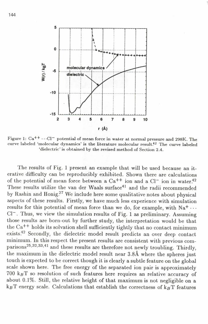
Figure 1: Ca++ .. .Cl- potential of mean force in water at normal pressure and 298K. Thecurve labeled 'molecular dynamics' is the literature molecular result.42 The curve labeled

'dielectric'is obtained by the revised method of Section 2.4.

The results of Fig. 1 present an example that will be used because an it-erative difficulty can be reproducibly exhibited. Shown there are calculationsof the potential of mean force between a Ca ++ ion and a CI- ion in water .42These results utilize the van der Waals surface41 and the radii recommended

by Rashin and Honig.27 We include here some qualitative notes about physicalaspects of these results. Firstly, we have much less experience with simulationresults for this potential of mean force than we do, for example, with Na+ . ..CI-. Thus, we view the simulation results of Fig. 1 as preliminary. Assumingthose results are born-out by further study, the interpretation would be thatthe Ca++ holds its solvation shell sufficiently tightly that no contact minimumexists~2 Secondly, the dielectric model result predicts an over deep contactminimum. In this respect the present results are consistent with previous com-parisons25,32,33,41and these results are therefore not newly troubling. Thirdly,the maximum in the dielectric model result near 3.8A where the spheres justtouch is expected to be correct though it is clearly a subtle feature on the globalscale shown here. The free energy of the separated ion pair is approximately700 kBT so resolution of such features here requires an relative accuracy ofabout 0.1%. Still, the relative height of that maximum is not negligible on akBT energy scale. Calculations that establish the correctness of kBT features

--

145

require care.22,23,30Such methods are the topic of this paper.

2 Methods

Here we catalog the methodological results used below for solution of the Pois-son Eq. (1). Further discussion of the genesis of these results can be foundelsewhere:'u We first cast Eq. (1) as an integral equation, e.g.:

€(r)~(r) = ~(O)(r) + J [

(r - r'). V'€(r')

]~(r')d3r'.

47rIr - r'13(2)

The quantity ~(O)(r) is the electrostatic potential in the absense of the medium.Because the model assumes that €(r) has a sharp step at the molecular surfacethe integration on the right collapses to a 2-dimensional integration over themolecular surface. That molecular surface is defined as the boundary betweenthe molecular volume - modeled as the union of spherical volumes centeredon solute atoms - and the solution region. For r infinitismally outside themolecular surface, Eq. (2) provides a closed equation for ~(r) on the molecularsurface. Once ~(r) is obtained on the molecular surface, it can be used on theright side of Eq. (2) to construct the potential elsewhere.

From such solutions we construct the interaction part of the chemical po-tential of the solute as

I'lp(r) = G) J p(r)( iP,(r) - iP.(r)) d"r.(3)

The subscripts I and v indicate 'liquid' and 'vapor,' respectively, so that thisdifference is the electric work required to charge the solute in the liquid relativeto the vapor. This requires the solution of Eq. (2) twice, once for the liquidwith

€l(r) = €m + (€$ - €m) 7](r) ,

and once for the vapor with

(4)

€v(r) = €m + (1 - €m) 7](r). (5)

Here 7](r) is a step function that is one outside the molecular volume and zerootherwise; €$ is the dielectric constant of the solution and €m is an assigned'dielectric constant of the molecule.' The latter parameter is used to matchthe polarizability of the solute. The formulation Eq. (2) makes it simple tomatch a given polarizability by adjustment of €m.41This is because the kernelis proportional to the electrostatic potential due to a surface dipole density.

146

Thus, we perform calculations with ev(r) and with ~(O)(r) chosen to describea uniform external electric field. The induced electrostatic pot~ntial in thefar field is associated with the induced dipole moment. The corrdation of theinduced dipole moment with the external fidd strength provides the modeledmolecular polarizability.

2.1 Rules for coarse direct calculations

A discretized version of Eq. (2) is

Es~(ra) = ~(O)(ra) + L wa/3~(r/3)'/3

(6)

Here ra is the a-th 'plaque point' - a point on the molecular surface obtainedby a uniform sampling, for example by exploiting either quasi-random numberseries or 'good lattice' procedures~3-48 The plaques are defined as the Voronoipolyhedra of the plaque points on the nonburied surface of each sphere. Thematrix of coefficients wa/3 can be obtained as follows:

R(S/3)2(Es - em) "" (ra - r;). IiiWa/3= M ( ) L..t

I 13'

S/3 {iEI3} ra - ri

a t= {3, (7)

and1

(Es - Em

) "" -1/2Waa= /0 M(s) L..t (1 - cost?ia) .2y 2 a{i~a}

These are Monte Carlo estimates of plaque integrations. Further details canbe found elsewhere~l The set of sampling points that are within the plaque {3is denoted by {i E {3}. M (s /3) is the number of points on the sphere s/3 thatsupports plaque {3. In Eq. (8), t?ia is the angle between the surface normalsat plaque point a and the sampled point i. That formula arranges to usesample points outside the plaque to calculate the solid angle subtended bythat plaque at the plaque point. The purpose is to reduce the variance of theMonte Carlo estimate. All sample points on the surface of the sphere thatsupports plaque a should be used in the estimation. But whether any samplepoint resides on plaque a depends on resolution of buried surface because theplaque boundaries sometimes follow the boundaries between the exposed andburied surface.

For accurate calculations on small molecule solutes, we have found thatthe computational time is dominated by the Monte Carlo effort. Thus, weuse these formulae differently to avoid some of that effort. We use Eq. (7)

(8)

"',

147

with no Monte Carlo sample in addition to the plaque point; these formulaeconstitute one point estimates then. However, the set of plaque points isnow a larger set, of equidistributed surface points, elements of a fine lattice.We form the equations to be analyzed by contraction of that description toone based upon coarse plaques constructed from an initial sequence of thefine lattice points. We then require the equality of the potential at all finelattice points residing on the same coarse plaque. This requirement resultsin an overdetermined system. This system is analyzed with a singular valuedecomposition to obtain the plaque potentials that minimize the mean squareresidual of those equations~8

The advantages of this approach are that much of the Monte Carlo ef-fort can be avoided and that some account is taken of the spatial variationof 4>(O)(r) within a coarse. plaque. The principal disadvantage is that thisapproach requires more memory and this disadvantage can be severe.

2.2 Rules for Gauss-Seidel iteration

Here we give the rules used in our iterative calculations. We begin with anapproximate solution 4>(ra). That approximation is then updated in placeaccording to

4>(ra) +- (Es - waa)-l

{4>(O)(ra) + L wa,B4>(r,B)

},B:ta

(9)

sequentially for all Q'. In this calculation the plaque points are the points ofthe fine lattice. Because that set of points is expected to be large, the off-diagonal coefficients wa,Bare evaluated 'on the fly' using Eq. (7) but no MonteCarlo sample in addition to the plaque point. Our experience is that accurateevaluation of the diagonal coefficients Waa is important, so we evaluate themat an initial stage of the calculation and store them for later use.

These methods were applied to the calculation of the pair potential ofthe mean forces between a Ca++ and a CI- in water. It was found that

the Gauss-Seidel iteration scheme converged almost always, but diverged inrare but reproducible circumstances. A necessary and sufficient condition forthe convergence of Gauss-Seidel iteration is that the spectral radius of theiteration matrix must be less than one~9 Plotted in Fig. 2 are the eigenvaluesof the Gauss-Seidel iteration matrix for the Ca++ . . . CI- problem for the caseof r = 3.7Awith 36 plaque points. One eigenvalue is much greater than one.Also plotted there are eigenvalues of the Gauss-Seidel iteration matrix for thesame circumstances except that matrix elements were obtained by a modified

1

148

method described below. All eigenvalues are now substantially less than one.Using the corrected methods the divergences have not been observed.

2.3 What we did to fix the problem

It was when those Monte Carlo efforts were economized that iterative diver-

gence occasionally presented a problem. Furthermore, the diagonal matrixelements are always calculated the same way. This suggests that the observeddifficulty was due to the one-point estimate of the off-diagonal elements usedwhen the iterative calculation was implemented.

The estimate Eq. (7) will have a larger variance the closer the point ra toplaque {3. Thus, it is reasonable to suspect those matrix elements correspondingto close 0:{3. It was verified that this suspicion is correct by replacing wa{3by w{3{3whenever ra is on a different sphere than plaque {3 and Ira - r{31<2R( S(3)/-..; M (s(3). This is a statistical estimate of the radial extent of plaqueson center s{3. This unsatisfying maneuver eliminated the divergence.

A geniune solution is to implement a Monte Carlo calculation of thosematrix elements Wa{3identified as potentially problematic. For ra close toplaque {3, an approach like that of Eq. (8) using points sampled outside theplaque would be most appropriate. But for ra far from plaque {3, it would benatural to use points on the plaque. That we could use either approach whenthe point r a is not on the plaque is justified by the relation

J [(r - r'). V"E;r')

]d3r' = 0,

471"Ir - r'l(10)

valid for r outside the sphere. This is an application of Gauss's law. Thus wecould estimate the required integral using either points on the plaque {3or ona complementary spherical surface. Using 1/2 of each estimate is an exampleof the method of antithetic variates:5o

- R(s{3 )2(E3 - Em)

[L (ra - ri) . Iii - L (ra - ri) . Iii

]Wa{3 -

I 13 I 13

'

2M S r - r. r - r.( (3) {iE{3} a. {i~{3} a .

(11)

This effort is expended only when ra is on a different sphere than plaque {3

and Ira - r{31< 2R(s{3)/VM(s{3).

J

-

149

~asc:-tnasE-

I . . . . I . . . . ~ . . . . . .

0.2 ~ t 1 ~ r...~I , ! II , I I .I , 1 I .

O.1 ~" I t t tI I I 0

I I I :

0.0 1 o"""""""'-r"""""""""""""""""""'1"""""""""""""""""""", ,...I , , of, I , .

-0.1 I :...t ~ ~ ~I I I I, I I II I I I

-0.2 1 + ] """"""""""""'f"""""""""""""""""""~"J . . . . I . . . . ~ . . . . l

-2.0 -1.5 -1.0 -0.5 0.0

Real

0.08. ! ill 0 I . . .

I I I I i I I I I0.06 J.."""""'+-"""""

,I..""""-f""""""""!""""""""I"""""'"..+ + 1,""""""'+"""""'"I !.,!, .

I , I I I I ! I iI , I . . . . I .

O.04 ~"""""""r"""""""""""""""'I Q'I""""""'".'1 t""""""""I , t t............! ! ! Ii; ; I I

I , Ii' 1 ill0.02 1 1 + 1 1 + 1 + +..............

::>. Ii f i i i I 101L. . I I . . ; I I !

as !! lot) 0; ! , i

.E 0.00 "~"""l"""""""I t""""""""I""o""'~"""'J"""""""'1 t +...........tn i i ! j. r ; i I IIas i i I i I ! ! 0 I

E -0.02 t"""""""'j r \ j t""""""""I t t.............. ; ! . . . , ! !i i I i j i j I i-0 04 I """"""'~"""""""" I""""""""+"""-'-& I""""""""!""""""+ ! t t............... r'. . ..,

i i I I ! i i i II I I I ! ! i ! !

-0.06 ~ i i + + ""'"..j t + t j.............i i I I i j i i II I i I I 0 I ! I Ii I I ~ I I ! t I

-0.04 -0.02 0.00 0.02 0.04

Real

-0.08

Figure 2: Upper panel: Eigenvalues of the Gauss-Siedel iteration matrix obtained as de-scribed in Section 2.2 for 36 plaques on the Ca++ ... CI- ill-ion for r =3.7A. One eigen-value is much further from the origin than 1.0. Lower panel: Eigenvalues of the Gauss-Siedel

iteration matrix obtained by the revised approach described in Section 2.3.

150

3 Deprotonationof monosilicic acid in water

As an application of the methods developed in the previous sections we willtreat the deprotonation of monosilicic acid in water at 298K

Si(OH)4 ~ Si(OH)30- + H+. (12)

The monosilicic acid molecule and anion are depicted in Fig. 3. The equilibriumratio is

[{ = [Si(OHhO-] [H+][Si(OH)4]

(13)

with concentrations in molar units. The quantity we seek is the free energy ofreaction

~G(O) = - RT In [{ (14)

measured to be 13.5 kcal/mol~1-53This is a helpful example for several reasons. Acid-base equilibria are

an important application of these models in molecular biophysics. Addition-ally, these solutes have not be treated previously by these methods. Thus,the expectations for the radii-parameters required can be tested outside theconventional parameterization suite of solutes.

3.1 Solution thermodynamic formulation

It is more physical34 to consider the reaction

Si(OH)4 + H2O ~ Si(OHhO- + H3O+. (15)

The reaction described this way does not result in a net loss of chemical bondsand this is likely the case in water!34 The ratio

j{ = [Si(OH)30-] [H3O+][Si(OH)4] [H2O]

(16)

is then dimensionless. This equilibrium ratio may be obtained as34

k(T) = k(O)(T) exp [-~~J/X) / RT] , (17)

where k(O)(T) is the ideal gas result obtainable from standard formulae,54 and

(x) (x) A (x) ~ (x) ~ (x)~~JL = ~JLH30+ + ~JLSi(OHhO- - JLH2o- JLSi(OH)4' (18)

151

Table 1: Partial charges for Si(OHh and Si(OH)JO-.

!< and i< are related by i< = !</[H2O] and the free energy of reaction is simply

~G(O) = -RTlnj{ - RTln[H2O]. (19)

We assume that the solute concentrations are sufficiently low that the formalconcentration of H2O is satisfactory.

3.2 Electronic structure results on the isolated molecules

All electronic structure calculations were performed using the GAUSSIAN-92 program.55 Two different quantum mechanical methods were employed:Hartree-Fock (HF), and HF followed by a second-order order Moller-Plesset(MP2) correlation energy correction. Two different basis sets were used: 6-31G( d) [also denoted 6-31G*], and 6-31G++(2d). The "(d)" and "(2d)" de-notes that the 6-31G basis is supplemented by one and two sets of polar-ization56 d-functions, respectively, on the heavy (non-hydrogen) atoms. The"++" denotes that the basis is supplemented by diffuse57 functions. Togetherthe quantum mechanical method and basis set specifies a theoretical model,e.g., Sauer58 has performed HF /6-31G( d) calculations on monosilicic acid. Theoptimized geometries for H2O, HaO+, Si(OH)4 and Si(OH)aO- were deter-mined by analytic gradient techniques using the HF /6-31G( d) model. Thestructures found for monosilicic acid and its anion are shown in Fig. 3. Thebond distance and angle for H2O is 0.947 Aand 105.50°, respectively comparedto the experimental values59 of 0.957 Aand 104.5°, respectively. The calculatedvalue for all three H-O-H bond angles for HaO+ is 113.06°. Teppen et al.6ohave examined the effects of basis set size and electron correlation corrections

Atom Si(OH)4 Si(OH)aOSi 1.62 1.5201 -0.90 -0.8902 -0.90 -0.9003 -0.90 -0.9204 -0.90 -1.06HI 0.49 0.44H2 0.49 0.41H3 0.49 0.41H4 0.50 -

,..

152

Table 2: Partialcharges forH2O and H30+,

on the properties of monosilicic acid. For a 6-31G( d) basis, they60 find that theMP2 bond lengths for Si-O and O-H were 0.022 and 0.023A larger, respectivelythan the HF values and the MP2 Si-O-H angle decreased 2.90 from the HFvalue. For the HF method, they6O also find that the MC6-311G(2d,2p)61 bondlengths for Si-O and O-H were 0.007 and 0.009A smaller than the 6-31G( d)values and the MC6-311G(2d,2p) Si-O-H bond angle increased 1.30 from the6-31G( d) value. For the present work these differences are acceptable, andHF /6-31G( d) was used to optimize geometries.

To obtain atom-centered charges (Tables 1 and 2) necessary for the sol-vation energy calculation, a fit of the HF /6-31G( d) electrostatic potential(CHELPG62) was performed. Harmonic vibrational frequencies and rota-tional constants were computed with the HF /6-31G( d) model and were usedto compute the partition functions in Eq. (17). Since the HF method over-estimates frequencies, the computed values were scaled by 0.88.63 The elec-tronic ground state energies, Eo, (Table 3) were calculated by optimizing themolecules with the MP2/6-31G( d) model. The calculation of polarizability,ii = (axx + ayy + azz )/3, is sensitive to the basis set. For H2O at the HF/6-31G( d) geometry, ii = 0.70, 0.90, 0.90, and, 1.06A 3, calculated with the 6-31G( d), 6-31+G( d), 6-31G(2d), and 6-31++G(2d) basis sets, respectively. The6-31++G(2d) value agrees reasonably well with another HF calculation~4 ii =1.17A3. The experimental value65,66 for H2O, ii = 1.44A3, was used in thesolvation calculations for both H2O and H3O+. For Si(OH)4 and Si(OH)aO-,ii was calculated with the HF /6-31G++(2d) model using the HF /6-31G( d)geometries. These values were scaled by 1.36, the ratio of the experimentaland HF /6-31G++(2d) ii values for H2O. The scaled values (Table 3) were thenused in the solvation calculations.

3.3 Results for the deprotonation of monosi/icic acid

Three different calculations were performed for the free energy of deprotona-tion, Eq. (12). The first calculation did not include molecular polarizability,nor spheres on the H atoms of Si(OH)4 and Si(OH)30-, The second calcula-tion included molecular polarizability, but again not spheres on the H atoms.

Atom H2O H3O+0 -0.82 -0.62

H 0.41 0.54

153

117.0°

Figure 3: Monosilicic acid molecule (upper) and anion (lower) established by the electronicstructure calculations of Section 3.2

'.

154

Table 3: Electronic energies and polarizabilities.

The final calculation included both molecular polarizability and spheres onevery atom of Si(OH)4 and Si(OHhO-. This sequence of calculations reflectsour chronological approach to this system starting with the simplest model,gradually adding more complications, and gradually refining the values of theparameters used. This approach also gives helpful information on the sensitiv-ity of the calculation to the empirical parameters used.

The evaluation of the vibrational, rotational, and translational partitionfunctions of the isolated molecules on the basis of the electronic structure

results leads to a multiplicative contribution of 1.30 to the equilibrium ra-tio of Eq. (17). The change in the electronic energy ~Eo was found to be197.5 kcalfmol.

In all of the calculations the water and hydronium ions were treated assingle spheres of radius 1.6A.on the 0 atom. A molecular dielectric constant €m

was 2.42. This reproduces the polarizability of the water molecule~4,65,66 Thesolution dielectric constant was €$ = 77.4 appropriate to water at 298K and1.0gf cm3. The calculation of the excess chemical potential of solvent speciesused 186 coarse lattice points and 936 fine lattice points. Ten Gauss-Seideliteration passes were applied to the coarse solution in all calculations. Thedifference in excess chemical potential between the hydronium ion and waterwas found to be -107 kcalfmol. All calculations on Si(OH)4 and Si(OHhO-used 36 coarse lattice points and 936 fine lattice points on each sphere.

The first calculations for Si(OH)4 and Si(OHhO- used a sphere of radius1.8A. on the each Si atom and a sphere of radius 1.651 on each 0 atom.€m = 1.0 was adopted, thus ignoring the polarizability of the molecule. Thedifference in excess chemical potential was found to be -49.6 kcalfmol. Thiscalculation gives 38.3 kcalfmol for the change in free energy for Eq. (12), inpoor agreement with experiment.

In the next calculation a sphere of radius 1.8A. was centered on the eachSi atom and a sphere of radius 1.601 on each 0 atom. €m =2.95 and 3.40were assigned to the Si(OH)4 and Si(OH)30- molecules, respectively. These

Molecule Eo (hartree) a (A3)Si(OH)4 -590.89169 6.9

Si(OHhO -590.29838 7.4

H2O -76.01075 1.44

H3O+ -76.28934 1.44

155

values match the estimated molecular polarizabilities discussed in the previoussection. The difference in excess chemical potential was found to be -57.9kcalfmol, which gives 30.0 kcalfmol for the change in free energy for Eq. (12).This improves upon the calculation which ignored the polarizability of Si(OH)4and Si(OH)JO- but still differs from experiment by more than a factor of two.

The final calculation had spheres on every atom of the solute molecules.The 0 atoms were given radii of 1.4A, the Si atoms were given radii of 1.8A,and the H atoms were given radii of 1.3A. Values of 3.10 and 3.55 were used forthe em of Si(OH)4 and Si(OH)30-, respectively. Again these values were de-termined to match the polarizability of the molecules. The difference in excesschemical potential between Si(OH)4 and Si(OH)JO- was -68.1 kcalfmol. Thiscalculation gives 19.8 kcalfmol for the change in free energy for the deproto-nation of Si(OH)4 in water, a much improved agreement with experiment.

4 Conclusions

The iterative divergence occasionally encountered in the calculation of theCa++ . . . CI- pair potential of mean force was due to inaccuracies of the asymp-totic approximations used for the matrix elements for accidentally close bound-ary elements on different atomic spheres. This problem is cured by checking forboundary element pairs closer than the typical spatial extent of the boundaryelements and for those pairs performing an 'in-line' Monte Carlo integrationto evaluate the required matrix elements. These difficulties are not expectedand have not been observed when only a direct solution is considered.

These methods can give a reasonable description of the free energetics ofthe deprotonation of monosilicic acid in water. A modeled solute polarizabilityand spheres on hydroxyl protons have been found to be important in achievinga reasonable agreement between model and experiment. The discrepancy re-maining provides a suggestion of more specific solute-solvent interaactions. Ithas been noted previously41 how specific molecular solvation structure can bereintroduced into these models. Those ideas for integrating-out solvent degreesof freedom suggest the electronic structure calculations should be performedon complexes of the solutes of interest plus a probe water molecule:u Thoseapproaches will require a substantially larger computational effort.

The necessity of better treatment of the molecular solvation structure isalso clear in the example of Ca++ . . . CI-. The probe water molecule approachmentioned above would help here too but would require accurate, rapid calcu-lations on larger, more complicated solution complexes. It is hoped that themethods developed here will make such calculations feasible.

156

Acknowledgements

SAC acknowledges the support of Associated Western Universities. We thankC. O. Grigsby, P. J. Hay, and R. L. Martin for helpful comments.

References

1. A. A. Rashin, J. Phys. Chern. 94, 1725 (1990).2. B. Honig, K. Sharp, and A.-S. Yang, J. Phys. Chern. 97, 1101 (1993).3. S. Miertus, E. Scrocco, and J. Tomasi, Chern. Phys. 55, 117 (1981).4. J. Warwicker, and H. C. Watson, J. Mol. Bioi. 157, 671 (1982).5. M. K. Gilson, A. Rashin, R. Fine, and B. Honig, J. Mol. Bioi. 183, 503

(1985).6. R. J. Zauhar, and R. S. Morgan, J. Mol. Bioi. 186, 815 (1985).7. I. Klapper, R. Hagstrom, R. Fine, K. Sharp, and B. Honig, PROTEINS:

Structure, Function, and Genetics 1, 47 (1986).8. M. .K. Gilson, K. A. Sharp, and B. H. Honig, J. Compo Chern. 9, 327

(1987).9. J. L. Pascual-Ahuir, E. Silla, J. Tomasi, and R. Bonaccorsi, J. Compo

Chern. 8, 778 (1987).10. A. A. Rashin, and K. Namboodiri, J. Phys. Chem., 91, 6003 (1987).11. M. K. Gilson, and B. H. Honig, PROTEINS: Structure, Function, and

Genetics 3, 32 (1988).12. R. J. Zauhar, and R. S. Morgan, J. Compo Chern. 9, 171 (1988).13. M. E. Davis, and J. A. McCammon, J. Compo Chern. 10, 386 (1989).14. B. J. Yoon, and A. M. Lenhoff, J. Compo Chern. 11, 1080 (1990).15. A. H. Juffer, E. F. F. Botta, B. A. M. van Keulen, A. van der Ploeg, and

H. J. C. Berendsen, J. Compo Phys. 97, 144 (1991).16. A. Nicholls, and B. Honig, J. Compo Chern. 12,435 (1991).17. B. Wang, and G. P. Ford, J. Chern. Phys. 97, 4162 (1992).18. H. Oberoi, and N. M. Allewell, Biophys. J. 65, 48 (1993).19. H.-K. Zhou, Biophys. J. 65, 955 (1993).20. V. Mohan, M. E. Davis, J. A. McCammon, and B. M. Pettitt, J. Phys.

Chern. 96, 6428 (1992).21. T. J. You, and S. C. Harvey, J. Compo Chern. 14,484 (1993).22. T. Simonson, and A. T. Brunger, J. Phys. Chern. 98,4683 (1994).23. S. C. Tucker, and E. M. Gibbons, Structure and reactivity in aqueous

solution: Characterization of chemical and biological systems, edited byC. J. Cramer and D. G. Truhlar, ACS Symposium Series 568,198 (1994).(ACS, Washington DC, 1994).

157

24. J. E. Snitzer, and K. C. Lambrakis, J. Theor. Bioi. 152, 203 (1991).25. A. A. Rashin, J. Phys. Chern. 93, 4664 (1989).26. G. P. Ford, and B. Wang, J. Arn. Chern. Soc. 114, 10563 (1992).27. A. A. Rashin, and B. Honig, J. Phys. Chern. 89,5588 (1985).28. C. Lim, D. Bashford, and M. Karplus, J. Phys. Chern. 95, 5610 (1991).29. K. Sharp, A. Jean-Charles, and B. Honig, J. Phys. Chern. 96, 3822

(1992).30. R. Bharadway, A. Windemuth, S. Sridharan, B. Honig, and A. Nicholls,

J. Compo Chern. 16, 898 (1995).31. B. Jayaram, R. Fine, K. Sharp, and B. Honig, J. Phys. Chern. 93, 4320

(1989).32. L. R. Pratt, G. Hummer, and A. E. Garda, Biophys. Chern. 51, 147

(1994).33. G. J. Tawa and L. R. Pratt, Structure and reactivity in aqueous solu-

tion: Characterization of chemical and biological systerns, edited by C.J. Cramer and D. G. Truhlar, ACS Syrnposiurn Series 568, 60 (1994).(ACS, Washington DC, 1994).

34. G. J. Tawa and L. R. Pratt, J. Am. Chern. Soc. 117, 1625 (1995).35. R. M. Levy, M. Belhadj, and D. B. Kitchen, J. Chern. Phys. 95, 3627

(1991).36. P. E. Smith, and W. F. van Gunsteren, J. Chern. Phys. 100,577 (1994).37. S. W. Rick, and B. J. Berne, J. Arn. Chern. Soc. 116, 3949 (1994).38. G. Hummer, L. R. Pratt, and A. E. Garda, LA-UR-95-1161, J. Phys.

Chern. in press (1995).39. G. Hummer, L. R. Pratt, and A. E. Garda, LA-UR-95-1612, J. Phys.

Chern. in press (1995).40. A few recent examples: (a) N. Rosch, and M. C. Zerner, J. Phys. Chern.

98, 5817 (1994); (b) A. A. Rashin, M. A. Bukatin, J. N. Andzelm, andA. T. Hagler, J. Biophys. Chern. 51, 375 (1994); (c) C. Chipot, L. C.Gorb, and J. L. Rivail, J. Phys. Chern. 98, 1601 (1994); (d) J. L. Chen,L. Noodleman, D. A. Case, and D. Bashford, J. Phys. Chern. 98, 11059(1994); (e) D. J. Tannor, B. Marten, R. Murphy, R. A. Friesner, D.Sitkoff, A. Nicholls, M. Ringhalda, W. A. Goddard, and B. Honig, B. J.Am. Chern. Soc. 116, 11875 (1994).

41. L. R. Pratt, G. J. Tawa, G. Hummer, A. E. Garda, and S. A. Corcelli,(July, 1995): "Boundary Integral Methods for the Poisson Equation of

. Continuum Dielectric Solvation Models." LA-UR-95-2569.42. E. Guardia, R. Rey, and J. A. Padro, J. Chern. Phys. 99, 4229 (1993).43. J. M. Hammersley and D. C. Handscomb, Monte Carlo Methods, (Chap-

man and Hall, London, 1964). pp. 31-36.

158

44. H. 1. Keng, and W. Yuan, Applications of Number Theory to NumvericalAnalysis, (Springer-Verlag, NY, 1981).

45. A. Lubotzky, R. Phillips, and P. Sarnak, Comm. Pure Appl. Math. 39,S149 (1986); Comm. Pure Appl. Math. 40, 40, 401 (1987).

46. R. F. Tichy, J. Compo Appl. Math. 31, 191 (1990).47. H. Niederreiter, Random Number Generation and Quasi-Monte Carlo

Methods, (SIAM, Philadelphia, 1992).48. W. H. Press, S. A. Teukolsky, W. T. Vetterling, and B. P. Flannery,

Numerical Recipes, The Art of Scientific Computing, 2nd edition, (Cam-bridge University Press, NY, 1992). §7.7.

49. J. C. Strikwerda, Finite Difference Schemes and Partial DifferentialEquations, (Wadesworth & Brooks/Cole, Pacific Grove, California,1989).

50. J. M. Hammersley and D. C. Handscomb, Monte Carlo Methods, (Chap-man and Hall, London, 1964). pp. 60-66.

51. R. M. Garrels, and C. L. Christ, Solutions, Minerals, and Equilibria,(Freeman, Cooper & Company, San Francisco, 1965).

52. R. K. Her, The Chemistry of Silica. Solubility, Polymerization, Col/oidand Surface Properties, and Biochemistry (Wiley, New York, 1979). pp.180-181.

53. J. R. Rustad, and B. P. Hay, Geochim. Cosmochim. Acta 59, 1251(1995).

54. D. A. McQuarrie, Statistical Mechanics (Harper and Row, New York,1976). Chapter 8.

55. M. Frisch, G. W. Trucks, M. Head-Gordon, M.; P. M. W. Gill, M. W.Wong, J. B. Foresman, B. G. Johnson, H. B. Schlegel, M. A. Robb, E. S.Replogle, R. Gomperts, J. 1. Andres, K. Raghavachari, J. S. Binkley, C.Gonzales, R. L. Martin, D. J. Fox, D. J. Defrees, J. Baker, J.; J. J. P.Stewart, and J. A. Pople, GA USSIAN 92, Revision A; Gaussian Inc.:Pittsburgh, PA, 1992.

56. M. Frisch, J. A. Pople, and J. S. Binkley, J. Chem. Phys. 80, 3265(1984).

57. T. Clark, J. Chandrasekhar, G. W. Spitznagel, and P. v.R. Schleyer, J.Compo Chem. 4, 294 (1983).

58. J. Sauer, J. Phys. Chem. 91,2315 (1987).59. G. Herzberg, Molecular Spectra and Molecular Structure. III. Electronic

Spectra and Electronic Structure of Polyatomic Molecules, (Van NostrandReinhold: New York, 1966)-

60. B. J. Teppen, D. M. Miller, S. Q. Newton, and L. Schafer, J. Phys.Chem. 98, 12529 (1994).

r-159

61. A. D. McLean,and G. S. Chandler, J. Phys. Chern. 72, 5639 (1980).62. C. M. Breneman, and K. B. Wiberg, J. Compo Chern. 11, 361 (1990).63. W. J. Hehre, 1. Radom, P. v.R. Schleyer, and J. A. Pople, Ab Initio

Molecular Orbital Theory, (Wiley, New York, 1986). p. 236.64. G. P. Arrighini, C. Guidotti, and O. Salvetti, J. Chern. Phys. 52, 1037

(1970).65. F. H. Stillinger, in Studies in Statistical Mechanics VIII, The Liquid

State of Matter: Fluids, Simple and Complex (North-Holland, NewYork,1982).

66. S. P. Liebmann, and J. W. Moskowitz, J. Chern. Phys. 54,3622 (1971).