14–17 August 2000 Denver, Colorado - Old Dominion …mln/ltrs-pdfs/NASA-aiaa-2000-4321.pdf ·...

AIAA 2000-4321Steady–State Computation ofConstant Rotational RateDynamic Stability DerivativesMichael A. ParkGeorge Washington UniversityJoint Institute for the Advancement of Flight Sciences (JIAFS)

Lawrence L. GreenNASA Langley Research Center, Hampton, Virginia

18th Applied Aerodynamics Conference14–17 August 2000Denver, Colorado

For permission to copy or to republish, contact the American Institute of Aeronautics and Astronautics,1801 Alexander Bell Drive, Suite 500, Reston, VA, 20191-4344.

American Institute of Aeronautics and Astronautics1

AIAA-2000-4321

STEADY–STATE COMPUTATION OF CONSTANT ROTATIONAL RATEDYNAMIC STABILITY DERIVATIVES

Michael A. Park*

George Washington University Joint Institute for the Advancement of Flight Sciences (JIAFS)[email protected]

Lawrence L. Green†

NASA Langley Research Center, Hampton, [email protected]

AbstractDynamic stability derivatives are essential to

predicting the open and closed loop performance,stability, and controllability of aircraft. Computationaldetermination of constant-rate dynamic stabilityderivatives (derivatives of aircraft forces and momentswith respect to constant rotational rates) is currentlyperformed indirectly with finite differencing ofmultiple time-accurate computational fluid dynamicssolutions. Typical time-accurate solutions requireexcessive amounts of computational time to complete.Formulating Navier-Stokes (N-S) equations in arotating, noninertial reference frame and applying anautomatic differentiation tool to the modified code hasthe potential for directly computing these derivativeswith a single, much faster steady-state calculation. Theability to rapidly determine static and dynamic stabilityderivatives by computational methods can benefitmultidisciplinary design methodologies and reducedependency on wind tunnel measurements. TheCFL3D thin-layer N-S computational fluid dynamicscode was modified for this study to allow calculationson complex three-dimensional configurations withconstant rotation rate components in all three axes.These CFL3D modifications also have directapplication to rotorcraft and turbomachinery analyses.The modified CFL3D steady-state calculation is a newcapability that showed excellent agreement with resultscalculated by a similar formulation. The application ofautomatic differentiation to CFL3D allows the staticstability and body-axis rate derivatives to be calculatedquickly and exactly.

*Graduate Student, NASA Langley Research Center,Multidisciplinary Optimization Branch, MS 159, Hampton, Virginia,Member AIAA†Research Scientist, Multidisciplinary Optimization Branch, MS159, Senior Member AIAA

Copyright 2000 by the American Institute of Aeronautics, Inc. Nocopyright is asserted in the United States under Title 17, U.S. Code.The Government has royalty-free license to exercise all rights underthe copyright claimed herein for government purposes. All otherrights reserved by the copyright owner.

IntroductionDynamic derivatives quantify the aerodynamic

damping of aircraft motions and are used to predict thelongitudinal short period, lateral pure roll, and lateralDutch roll behavior of the configuration. Analytical,empirical, and vortex lattice methods of estimatingthese derivative values are not suited to unconventionalconfigurations or high-speed, compressible flowsdominated by viscous effects. Evaluatingunconventional configurations is of growing interestdue to the design and analysis of next generationattack, transport, and reusable launch vehicles.Examples of these new, unconventional designs are theblended wing body and the X-33 configurations. Amethodology of using high fidelity, noninertial Eulerand Navier-Stokes (N-S) calculations gives improvedcapability in predicting these dynamic stabilityderivative values in compressible flow on conventionalor unconventional designs.

Due to cost and time limitations, it is impractical toconstruct and test numerous wind tunnel models duringinitial prototyping. Therefore, measurement of theeffects of aircraft dynamics on preliminaryconfiguration aerodynamic forces and moments islimited. The application of automatic differentiation toa noninertial reference frame Euler and N-S code haspotential for providing designers with insight, gainedfrom higher fidelity codes, into aircraft dynamics at thepreliminary design stage. This design stage is whencontrol surface size and preliminary control laws arebeing evaluated. Computational determination of thesederivatives is cheaper and faster than performing windtunnel measurements and will aid rapid prototypingand multidisciplinary design.

The modification of the CFL3D1 (ComputationalFluids Laboratory Three-Dimensional) computationalfluid dynamics (CFD) code to perform calculations ina noninertial, rotating reference frame has the potentialto reduce the reliance on forced-motion wind tunneland free-flight wind tunnel tests. Considerableprevious work performed on turbomachinery hasdemonstrated noninertial, rotating reference frame


fluid mechanics as a means to greatly reducecomputational time (for an example see Ref. 2). Kandiland Chuang3,4 have demonstrated noninertial referenceframe calculations for general motions on rollingaircraft stability problems. Limache and Cliff3 devisedan efficient scheme for the special case of steady-ratemotion and applied this technique to stability andcontrol work with a two-dimensional (2-D),unstructured grid code and the sensitivity equationmethod.

The noninertial modifications to CFL3D wereinitially validated in this study for a 2-D NACA0012airfoil case with comparisons to previously publishedresults by Limache and Cliff.5 The modified CFL3Dwas then applied to the full three-dimensional (3-D)Lockheed Martin Tactical Aircraft Systems—Innovative Control Effectors™ (ICE)‡ configuration6

(Fig. 1) with a turbulent Navier-Stokes calculation.

Technical ApproachThis study adopted the Limache and Cliff5

approach. There were two major aspects to this project.The first was modifying CFL3D to performcalculations in a rotating, noninertial reference frame.These CFL3D modifications included adding a sourceterm to the residual calculation and modifying theboundary and initial conditions. The second aspect wasthe application of ADIFOR7,8 (AutomaticDifferentiation in FORTRAN) to the latest parallelversion of CFL3D. This code was used to computederivatives of aircraft forces and moments with respectto the flow angles and constant rotational rates in theroll, pitch, and yaw axes. The application of ADIFORto the unmodified version of CFL3D has beenperformed successfully to calculate static stabilityderivatives9 (derivatives of aircraft forces and momentswith respect to angle of attack and angle of sideslip).

CFL3D IntroductionThe CFL3D code is a FORTRAN 77 (F77)

Reynolds-averaged thin-layer N-S flow solver forstructured-volume grids. CFL3D was written primarilyat NASA Langley Research Center and is undergoingcontinuous development and improvement. The codehas the ability to compute inviscid Euler, laminar N-S,and turbulent N-S calculations. The code employsparallelization by decomposing the computationaldomain into many separate blocks. These individualblocks are analyzed in separate processes thatcommunicate with each other by means of the MessagePassing Interface (MPI) standard. Analysis for this ‡ The use of trademarks or names of manufacturers in this report isfor accurate reporting and does not constitute an officialendorsement, either expressed or implied, of such products ormanufacturers by the National Aeronautics and SpaceAdministration.

study has been performed in an inviscid, Euler modeand a viscous mode with the N-S equations coupled tothe Spalart-Allmaras (S-A) turbulence model.1

CFL3D Noninertial Reference Frame ModificationsThere are two reference frames depicted in Fig. 2:

the inertial reference frame (denoted with upper-casesymbols) and the noninertial frame (denoted withlower-case symbols). The CFD grid (depicted as acube) is embedded in the noninertial reference frame.Positions relative to each of these two reference framesare quantified by three scalar quantities (X, Y, Z and x,y, z) that describe location along three orthonormal unitvectors (I, J, K and i, j, k). Note that bold type faceindicates vector symbols. The inertial frame is fixed inspace and the noninertial frame can translate and rotatewith the rotation described with three scalarcomponents (ωx , ωy, ωz) of the rotation vector ω . Thenoninertial frame and CFD grid follow a curved path(denoted as the curved, dashed arrow) as theysimultaneously translate and rotate.

Each of these coordinate systems has advantagesand disadvantages. An advantage of the inertial frameis that it is not moving (the existing stationary grid N-Sequations in CFL3D are only formulated fornonmoving frames). An advantage of the noninertialreference frame is that it moves with the CFD grid;therefore, the stationary grid formulation of theCFL3D N-S equations is already coded in this frame ofreference with local (lower-case) variables. Adisadvantage of the noninertial reference frame is thecurrent, stationary grid N-S equations are notformulated correctly because the CFD grid and itsassociated reference frame are rotating (e. g.,accelerating) in this study to simulate aircraftconstant-rate motion.

In order to correctly modify the stationary grid N-Sequations to calculate valid solutions with a translatingand rotating CFD grid, the relation between thedescriptions of the same point in both reference frames(b and B) must be sought. Note that all of thesederivations are performed at the instant in time whenthe unit normal vectors of both systems are parallel,which removes the necessity of a rotational coordinatetransform. Also, the noninertial reference frame istranslating and rotating at a constant rate; thereforeangular acceleration, ω& , is zero. A nonzero value of ω&can be included to model more general motions,3,4 butsuch was not the intention of this study.

There are two points in space of interest for thisderivation: The position of the noninertial frameorigin, C, expressed as a function of the inertialcoordinates (X, Y, Z) and a fluid particle, B and b,expressed in the inertial and noninertial coordinates (X,Y, Z and x, y, z), respectively. At any instant in time, itis very easy to express the relation of the position of a


point in both coordinate systems by addition ofvectors.

= +B C b (1)

The next step is to find the relationship between theinstantaneous velocity of a point expressed in bothcoordinate systems. The velocity is found bydifferentiating the expression for the vector relation ofposition, Eq. (1), with respect to time. Note that therewill be an added complexity to computing thederivative of any vector quantity expressed in thenoninertial frame, e. g., b, because the unit normalvectors (i, j, k) are changing as a function of time, dueto rotation. To find the derivative of b, the product ruleis used on the multiplication of the scalar components(x, y, z) and unit vectors (i, j, k). The relation betweenthe instantaneous derivatives of the unit vectorsand × bω is found by taking the limit on the derivativeas dt goes to zero.10

d d ddt dt dt

= +B C b(2)

= + + ×B C b bω& && (3)

Now that the velocity relationship, Eq. (3), hasbeen derived, the far-field boundary conditions of thenoninertial CFD problem can be discussed. For freestream boundary conditions, the fluid particles are atrest in the inertial frame; therefore their velocity,

∞B& ,

is zero. The expression for the fluid velocity at theCFD grid free stream boundary conditions is

∞b& . The

aircraft, the noninertial reference frame, and the CFDgrid are all translating together at a velocity,C& , whichis negative the free stream velocity, u∞. The boundary

values for ∞

B& and C& are substituted into Eq. (3),

which is rearranged to form Eq. (4).

∞ ∞∞= − ×b u bω& (4)

Therefore, the free stream boundary conditions canbe described as the combination of a uniform flowcomponent, u∞, and a rigid body rotation component,

∞×bω . The CFL3D boundary conditions at the near-

field or solid surface boundary conditions are notaffected in this noninertial formulation.

The expression for acceleration is computed bydifferentiating the velocity relation, Eq. (3).10 The timederivatives of the b and b& terms are determined in thesame fashion as the derivative of the b term wasderived in Eq. (3). This relation is valid for any vectorquantity expressed in a noninertial frame. Note that

theω& term is zero because the rotation rate is assumedto be constant in this steady-state formulation.

( )dd d ddt dt dt dt

×= + +

bB C b ω& &&(5)

( )= + + × + × + × + × ×B C b b b b bω ω ω ω ω&& && & &&& & (6)

( )2= + + × + × ×B C b b bω ω ω&& && &&& (7)

Now the acceleration of the origin of thenoninertial, grid-fixed reference frame, C&& , must besought. In this formulation, the noninertial referenceframe (Fig. 2) is following a curved path (the dashedarrow) through inertial space as it simultaneouslytranslates (C& ) and rotates (ω ). The origin of thenoninertial reference frame must accelerate to followthis curved path. The expression for the acceleration ofa grid that is moving in a curved path with constantrotation rate is

, ∞= × = × −C C C uω ω&& & && (8)

Note that this reference frame origin acceleration iszero when C& is parallel to ω.

Now that the C&& term is known, the expressions forthe difference between the accelerations computed inthe inertial frame and the noninertial frame (CFD grid)can be completed. This difference in acceleration iscomputed by subtracting the acceleration of a fluidparticle in the noninertial frame, b&& , from theacceleration of the same particle expressed in theinertial frame, B&& . By accounting for this difference in

acceleration (pseudo-acceleration, −B b&&&& ), equationsdescribing the motion of particles measured in anoninertial frame can correctly mimic the totalacceleration of these fluid particles in the inertialframe.

( )2∞− = × − + × + × ×B b u b bω ω ω ω&& &&& (9)

The goal is to model constant-rate CFD gridrotation and translation with a steady-state CFDcalculation. The difference in acceleration between aninertial and a noninertial frame of reference isemployed to form a source term correction to the N-Sequations in CFL3D. To illustrate the formulation ofthe source term, the existing implementation of thestationary grid N-S equations in CFL3D must beexamined. In the CFL3D code, the N-S equations areexpressed in a regular-spaced, Cartesian gridcoordinate system. The generalized grid coordinatesystem that defines the problem (x , y, z) is internallymapped by CFL3D to this regular-spaced Cartesian


grid (ξ, η, ζ) with a coordinate transform. The N-Sequations are written in the regular-spaced, Cartesiangrid coordinate system as1

ˆ ˆˆ ˆ ˆ ˆˆ ( ) ( ) ( )0v v v

t ξ η ζ− − −∂

+ + + =∂ ∂ ∂ ∂

F F G G H HQ(10)

where Q is a vector of the conserved variables. Theconserved variables are a combination of density, ρ,velocity components (u, v, w) and total energy per unitvolume, e. The vector Q is the conserved variables

divided by J.

[ ]1ˆ Tu v w eJ J

ρ ρ ρ ρ= =QQ (11)

The Jacobean (J) of the coordinate transformation fromthe Cartesian to the generalized coordinate system is

( )( )

, ,

, ,J

x y z

∂=

∂

ξ η ζ(12)

The inviscid flux terms are F, G, and H and the

viscous flux terms are Fv, Gv, and Hv. The F , G , H ,ˆ

vF , ˆvG , and ˆ

vH flux terms are created by dividing byJ in the same manner as Q was. For a nondeformingmesh (J is constant with respect to time), the solutionis advanced in time with the residual, R .

1 ( )RJ t

∂ =∂Q Q (13)

The residual is computed as

ˆ ˆˆ ˆ ˆ ˆ( ) ( ) ( )( ) v v vR

ξ η ζ

∂ − ∂ − ∂ −= − + + ∂ ∂ ∂

F F G G H HQ (14)

To permit noninertial calculations, a source term(S) is added to the standard CFL3D residualcalculation.

1 ( )RJ t

∂ = +∂Q Q S (15)

The source term is a vector with 4 nonzerocomponents (the continuity equation is not affected).

0T

x y z eS S S SJρ = S (16)

The momentum equation source terms (Sx, Sy, andSz) are the three components of the pseudo-acceleration( −B b&&&& ). The “work” done by these momentum sourceterms must be included in the energy equation. Theenergy equation source term (Se) is the dot product ofthe local velocity with the pseudo-acceleration.

The N-S equations in CFL3D are written inconservative form, so the vector source term for thefour momentum and energy equations must include thevolume of each computational cell ( 1J − ) and thedensity, ρ, of the fluid. The energy equation sourceterm is the dot product of the local flow velocity, b& ,with pseudo-acceleration,

( )( )( )( )( )( )

( )( )

0

2

2

2

2

x

y

z

Jρ

∞

∞

∞

∞

× × + × − ×

× × + × − × = × × + × − × • × × + × − ×

b b u

b b uS

b b u

b b b u

ω ω ω ω

ω ω ω ω

ω ω ω ω

ω ω ω ω

&

&

&

& &

(17)

where [ ]x y z=b and [ ]u v w=b& . For

additional papers on the source term equations andassociated physics of similar applications of thistheory, see Refs. 2–5. Refs. 4 and 5 also includereference frame angular and translation accelerationterms.

ADIFOR Automatic DifferentiationAutomatic differentiation is a technique for

augmenting computer programs with statements for thecomputation of derivatives. This technique relies onthe fact that every function, no matter howcomplicated, is executed on a computer as a(potentially very long) sequence of elementaryoperations such as additions, multiplications, andelementary functions (e. g., sine and cosine). Byrepeatedly applying the chain rule of differentialcalculus to the composition of those elementaryoperations, derivative information can be computedexactly and in a completely automated fashion.

The ADIFOR process is a technique that appliesthe chain rule of differentiation to propagate, equationby equation, derivatives of intermediate variables withrespect to the input variables. The ADIFOR tool hasbeen developed jointly by the Center for Research onParallel Computation at Rice University and theMathematics and Computer Sciences Division atArgonne National Laboratory. In general, to applyADIFOR to a given F77 code, the user is only requiredto specify those program variable names thatcorrespond to the independent and dependent variablesof the target differentiation. The ADIFOR tool thendetermines the variables that require associatedderivative computations, formulates the appropriatederivative expressions, and generates new F77 code forthe computation of both the original simulation and thespecified derivatives.


The modified version of CFL3D is able to computethe aircraft forces and moments as a function of thethree body-axis orthogonal components (p, q, and r) ofthe rotation vector. The application of ADIFOR to themodified version of CFL3D produced a code thatcomputed the forward mode derivatives of the aircraftbody-axis force and moment coefficients (CN, CA, CS,Cl, Cm, and Cn) with respect to the three body-axisrotation rates (p, q, and r) and the flow angles of attack(α) and sideslip (β).

The latest beta version of CFL3D employs dynamicmemory allocation and MPI libraries for ease of useand efficient, scalable parallelization. Theseimplementations are not standard F77 features, andtherefore previous releases of ADIFOR cannot handlethe code without manual preprocessing andpostprocessing. The latest release of ADIFOR 3.011 hasreduced or eliminated much of the manual processingassociated with the MPI libraries; techniques forhandling the dynamic memory allocation libraries arebeing developed.

Examples and ResultsThe two examples in this study were a 2-D Euler

study of NACA0012 airfoil and a 3-D turbulent N-Scalculation on the ICE configuration6 (Fig. 1). TheNACA0012 study will be detailed first, because it wasused for initial validation by comparisons to existingmethods.

NACA0012 Dynamic DerivativesThe NACA0012 study focused on the effect of

pitch rate on the coefficients of normal force (Fig. 3)and pitching moment (Fig. 4) at zero deg angle ofattack and zero pitch rate. The derivatives (CNq, Fig. 3,and Cmq, Fig. 4) of these force and momentcoefficients with respect to nondimensional pitch ratewere computed by the ADIFOR-generated, noninertialCFL3D code (CFL3D.NI.AD). The pitch ratederivatives are nondimensionalized by dividing by theairfoil chord and multiplying by two times the freestream velocity. The NACA0012 pitching momentcenter is located at the leading edge of the airfoil. Theconvergence history of the derivative values is shownin Figs. 3 and 4. The discontinuities in the derivativeconvergence history are due to mesh sequencing froma coarser to a finer mesh every 500 iterations. Amaximum of three levels of multigrid was employedon the finer meshes. The 2-D grid dimensions (49 ×13, 97 × 25, 193 × 49, and 385 × 97) are denoted foreach mesh sequencing level. The derivative values arecompared to results computed by a similar methodpublished by Limache and Cliff (SFLOW),5 a panelmethod (QUADPAN),12 and a vortex lattice method(VORLAX).13

These 2-D NACA0012 cases shown in Figs. 3 and4 were chosen for initial validation of CFL3D.NI.AD.To improve convergence, a blend of half standardCFL3D and half CFL3D low-Mach-numberpreconditioning was applied for the 0.1 Mach (Figs. 3aand 4a) case. This preconditioning option was notapplied to the 0.5 Mach (Figs. 3b and 4b) or 0.8 Mach(Figs. 3c and 4c) cases. Note that the CFL3D.NI.ADderivative values are in excellent agreement with theSFLOW values. For the 0.1 and 0.5 Mach cases, thedifferences between CFL3D.NI.AD and SFLOW,although small, are most likely due to the formulationdifferences between the flow solvers in CFL3D.NI.ADand SFLOW. The SFLOW code employs thehand-coded sensitivity equation technique and anunstructured grid discretization, whereasCFL3D.NI.AD is an automatically differentiatedstructured grid formulation.

The 0.8 Mach case (Figs. 3c and 4c) shows poorconvergence properties. The poor convergence ofCFL3D.NI.AD at 0.8 Mach may be due to theinteraction of a shock, the flux limiter implemented inCFL3D, and the automatic differentiation technique.The CFL3D smooth flux limiter1 tuned to κ = 1/3 wasemployed for the NACA0012 study. This poorconvergence may be due to the automaticdifferentiation technique attempting to formulate thecontinuous derivative of a shock and flux limiter,which does not have a continuous derivative. The 0.8Mach case is also the worst comparison to SFLOW.Only the final value for SFLOW is quoted in Ref. 5;therefore the SFLOW 0.8 Mach case may or may notbe fully converged. The convergence was notimproved by disabling multigrid calculations orperforming additional iteration cycles. At 0.8 Mach,the final value of CFL3D.NI.AD and SFLOW differ innormal force pitch rate derivative by 4.4% (Fig. 3c)and in pitching moment pitch rate derivative by 8.9%(Fig. 4c).

ICE Pathlines at Zero Rotational RateAfter CFL3D.NI.AD was validated by comparison

with SFLOW, the ICE configuration (Fig. 1) flowstructure was examined with pathlines. These pathlinesare shown to illustrate the changes in airflow structurewith increasing angles of attack. Pathlines for thestarboard half-span of the ICE configuration are shownin Fig. 5. The pathlines were seeded slightly ahead ofthe sharp leading edge (just outside the boundarylayer). The pathlines were computed from a full-spanN-S CFL3D solution on a grid with approximately 3million cells. These symmetric solutions in Fig. 5 werecalculated at 0.6 Mach, zero deg angle of sideslip, zerorotational rate, and various angles of attack. All ICECFL3D solutions in this study were computed with theS-A turbulence model at a Reynolds number of


2,490,000 per foot or 71,760,000 per meanaerodynamic chord. Three levels of multigrid wereused for the fine grid solution of the 0–15 deg angle ofattack cases and multigrid was disabled for the finegrid solution of the 20–30 deg angle of attack cases.

The structure of the symmetric flow depicted inFig. 5 aids interpretation of the subsequent figures,which depict force, moment, and stability derivativeinformation at these flight conditions. Note theattached flow at 5 deg angle of attack (Fig. 5a). Weakleading edge vortical flow was present at 10 deg angleof attack (Fig 5b). This initial leading edge vortexstructure gained strength at 15 deg angle of attack (Fig.5c). A vortex burst developed near the trailing edge at20 deg angle of attack (Fig. 5d). This vortex burststructure is identified by an abrupt streamwise increasein vortex diameter. The initial vortex burst structureintensified and moved forward at 25 and 30 deg anglesof attack (Fig. 5e and 5f).

ICE Forces, Moments, and Lateral DerivativesA summary of the figures depicting ICE forces,

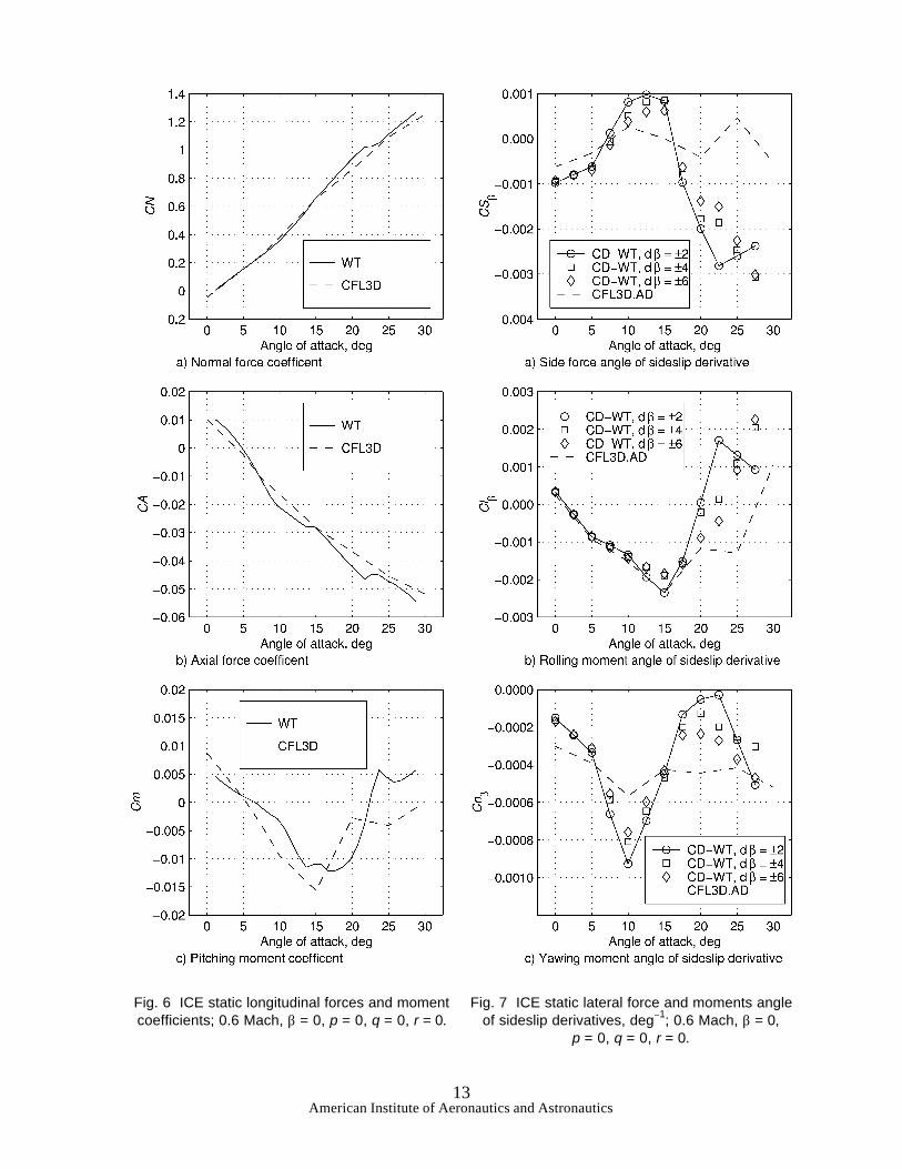
moments, and stability derivatives in this study isgiven in Table 1. Note that the elements assumed zerowould become significant at a nonzero angle ofsideslip, roll rate, or yaw rate. The ICE angle-of-attackderivatives are not presented in this study, but arepresented in Ref. 6 for 0–10 deg angles of attack. Theorientation of the six forces and moments, two flowangles, and three body-axis rotational rates is shown inFig. 1. Figure 6 shows a comparison of longitudinalforces and moment at 0.6 Mach, zero deg angle ofsideslip, and zero rotational rate. The momentreference center of the ICE is located longitudinally at39% of the mean aerodynamic chord (MAC) and adistance of 16% of the MAC below the body. Thecomparison is the wind tunnel data (solid line, WT)present in the ICE simulator database6 and CFL3D(dashed line). Coefficients of normal force, axial force,and pitching moment are shown in Fig. 6a, 6b, and 6c,respectively.

Figure 6 shows good agreement between WT andCFL3D. The WT data has more detail because it wasmeasured at approximately 1 deg increments, whichwere smaller than the 5 deg increments of the CFL3Dcalculations. There is no flow visualization informationavailable for the WT data, but the CFL3D pathlineswill be used to infer the effects of flow structure on theCFL3D calculations, which may also indicate the flowstructure effects on WT measurements. Note that theinitiation and strengthening of vortical flow between 5and 15 deg angles of attack (Fig. 5a–5c) increased thenormal force (Fig. 6a). The increasing strength of thevortex flow and the forward movement of the burstlocation over the wing between 20 and 30 deg anglesof attack (Fig. 5d–5f), increased the pitching moment

(Fig. 6c) which resulted in static longitudinalinstability above 15 deg angle of attack. Note thatCFL3D captures the radical change in Cm measured byWT (Fig. 6c).

Figure 7 shows the comparison among the lateralangle of sideslip derivatives for threecentral-finite-difference estimates from wind tunneldata6 (CD-WT) and an ADIFOR-generated CFL3Dsolution (CFL3D.AD). The CFL3D.AD derivatives aredashed lines and the CD-WT derivatives are thesymbols with a central-finite-difference step of ±2, ±4,and ±6 deg angle of sideslip for the circle, square, anddiamond, respectively. The ±2 deg CD-WT data isconnected with solid lines because the smallestcentral-finite-difference step (±2) is presumed to be themost accurate of the three finite difference step sizesfor small sideslip disturbances. All three finitedifference step sizes are shown to give an indication ofthe nonlinearities or measurement noise in the windtunnel data. The derivatives in Fig. 7 are presented inthe units of deg−1.

The effects of the vortical flow structure (Fig. 5)can be seen clearly in the lateral force and momentsangle-of-sideslip derivatives (Fig. 7). The initiationand strengthening of vortical flow between 5 and 10deg angles of attack (Fig 5a and 5b) can be interpretedto have sharply influenced the angle-of-attack trends ofCSβ and Cnβ (Fig, 7a and 7c) computed by CD-WTand CFL3D.AD. Then, the derivatives CSβ and Cnβ(Fig. 7a and 7c) dramatically reversed angle-of-attacktrends above 10 deg angle of attack. The CFL3D.ADClβ (Fig. 7b) derivative showed excellent agreementwith CD-WT for 0 to 15 deg angles of attack. The Clβcomparison deteriorated at higher (20–30 deg) anglesof attack.

As angle of sideslip varies, each wing experiencesdifferent effective leading-edge sweep angles. Due tothe highly swept (65 deg) leading edge of the ICEconfiguration the vortical flow field over the wing maybe sensitive to changes in effective leading-edge sweepangle. Therefore, the calculation of a vortex burststructure that formed symmetrically at 20 deg angle ofattack (Fig. 5d) may be produced asymmetrically atlower (10–15 deg) angles of attack. An asymmetric,bursting vortex structure may have been responsiblefor the dramatically reversed angle-of-attack trends inthe lateral derivatives (Fig. 7). The ICE configurationdoes not have any vertical surfaces, so the magnitudeof CSβ and Cnβ (Fig. 7a and 7c) was reduced ascompared to a configuration with vertical surfaces. Thesmall magnitude of CSβ and Cnβ may have hinderedmeasurement accuracy and exacerbated comparison ofCD-WT with CFL3D.AD.


ICE Dynamic DerivativesFigures 8 and 9 show the dynamic derivatives

computed by the DYNAMIC14 code andCFL3D.NI.AD. The DYNAMIC code utilized striptheory and the results of the high-angle-of-attackstability and control prediction code HASC15,16 tocalculate the dynamic derivatives. The HASC codeemploys VORLAX13 and empirical corrections topredict configuration forces and moments at variousflow angles and rotational rates. The derivatives werecomputed at zero rotational rate, zero angle of sideslip,and various angles of attack. The CFL3D.NI.ADdynamic derivatives were computed assumingrotations about the moment center of the configuration,which is located slightly below the body. Thelongitudinal pitch rate derivatives CNq and Cmq areshown in Fig. 8a and 8d, respectively. The longitudinaldynamic derivatives were nondimensionalized bydividing by the mean aerodynamic chord (345 in.) andmultiplying by two times the free stream velocity.

The rolling moment dynamic derivatives Clp andClr are shown in Fig. 8b and 8e, respectively. Theyawing moment dynamic derivatives Cnp and Cnr areshown in Fig. 8c and 8f, respectively. The side forcedynamic derivatives CSp and CSr are shown in Fig. 9aand 9b, respectively. The lateral dynamic derivativeswere nondimensionalized by dividing by the wingspanb (450 in.) and multiplying by two times the freestream velocity. There was no forced, oscillatorymotion wind tunnel data for comparison.

Both codes, CFL3D.NI.AD and DYNAMIC,showed fairly good comparison. Both of theCFL3D.NI.AD pitch rate (q) derivatives (Fig. 8a and8d) show a local maximum or a minimum near 5 degangle of attack. Note that the CFL3D.NI.ADcalculation of Cmq (Fig. 8d) was consistently morenegative than the combined analytical and vortexlattice method of DYNAMIC and VORLAX. Thistrend agrees with those of both SFLOW andCFL3D.NI.AD when compared to VORLAX for the2-D NACA0012 case (Fig. 4).

The roll rate (p) derivatives (Figs. 8b, 8c, and 9a)also showed a reversal of angle of attack trends at 5deg angle of attack. The reversals of the q and pderivative trends at 5 deg angle of attack correspondedto the indication of vortical flow at 10 deg angle ofattack in Fig. 5b. These p derivatives also showedanother local extreme at 15–20 deg angle of attack,which was slightly below the indication of vortexbursting in the static pathlines (Fig. 5d). A roll ratecreates differential angles of attack on each wing,which may induce asymmetric vortical burst structuresat lower angles of attack than a zero-roll-ratesymmetric case.

The yaw rate (r) derivatives (Figs. 8e, 8f, and 9b)had consistent trends in angle of attack at 15 deg angle

of attack and lower. These trends became lessconsistent at 20, 25, and 30 deg angles of attack, whichcorresponded with the initial indication of a symmetricvortex burst structure in Fig. 5d.

The CFL3D.NI.AD differentiated flow solver hadconvergence difficulties at 20, 25, and 30 deg angles ofattack. The 30 deg angle of attack case never reached asteady-state value, so an average of the last 2 thousanditerations is presented. These convergence difficultiesmay have been due to the presence of bursting vortexstructures, with their inherent unsteadiness andincreased sensitivity to disturbances. These highangle-of-attack conditions may be more suitable to atime-accurate solution, but in the interest ofminimizing computational resource requirements, thatapproach was not attempted in this study.

ICE Pathlines at Nonzero Rotational RatesFigure 10 shows the ICE configuration at 0.3

Mach, 15 deg angle of attack and zero deg angle ofsideslip, performing velocity vector rolls at variousrotational rates. In these velocity vector rolls, therotation vector was parallel to the free stream velocityvector; this condition simulated a wind tunnelrotary-balance test. These solutions were computed bythe noninertial, modified CFL3D (CFL3D.NI) code.The rotational rate (Ω) was nondimensionalized bymultiplying by the wingspan b (450 in.) and dividingby two times the free stream velocity (u∞), with apositive rotational rate indicating the starboard wingwas descending. The 0.2 and 0.4 rotational rate cases(Fig. 10b and 10c) showed a much tighter vortex coreon the ascending, port wing than the descending,starboard wing. The 0.4 rotational rate case (Fig. 10c)depicted a vortex burst on the descending, starboardwing. From this point of view, the vortex wakes in Fig.10b and 10c appear to be converging, but actually werespiraling around the rotation vector.

ICE Rotary-Balance and Noninertial CFL3DComparison

Figure 11 shows a comparison of wind tunnelrotary-balance data6 (ROT-BAL, solid line) andCFL3D.NI (dashed line) at 0.3 Mach, 15 deg angle ofattack, and zero deg angle of sideslip. Mach 0.3 waschosen to simulate the incompressible conditions of thelow-speed, rotary-balance tests. The ICE configurationwas rotated about the moment center of theconfiguration, which is located slightly below thebody. The figure shows the change (∆) in force ormoment coefficient between cases nonrotating androtating about the velocity vector. The rotation rate (Ω)about the velocity vector was nondimensionalized bymultiplying by the wingspan b (450 in.) and dividingby two times the free stream velocity (u∞), with apositive rotational rate indicating the starboard wing


was descending. Note that nonlinear effects withrotational rate were modeled in CFL3D.NI.

The increase in normal force (∆CN, Fig. 11a) dueto rotation was very similar between ROT-BAL andCFL3D.NI. The change in axial force (∆CA, Fig. 11b)due to rotation was very similar in magnitude betweenROT-BAL and CFL3D.NI, but opposite in sign. Thechange in pitching moment (∆Cm, Fig. 11c) due torotation was assumed to be an even function ascalculated by CFL3D.NI, but ROT-BAL showedinconclusive trends. The change in side force (∆CS,Fig. 11d) due to rotation was assumed to be an oddfunction as calculated by CFL3D.NI, but ROT-BALshowed inconclusive trends. The change in rollingmoment (∆Cl, Fig. 11e) due to rotation was the bestlateral comparison of CFL3D.NI with ROT-BAL. Thechange in yawing moment (∆Cn, Fig. 11e) due torotation calculated by CFL3D.NI was much greater inmagnitude and opposite in sign of the ROT-BAL trend.

The nonlinear effects with rotational rate ascalculated by CFL3D.NI in Fig. 11 can be correlated tothe calculation of a vortex burst structure over thedescending wing as illustrated in Fig. 10b and 10c. Thedifference between ROT-BAL and CFL3D.NI(highlighted in Figs. 11b, 11c, and 11f) is currentlyunder investigation. A possible explanation ofROT-BAL asymmetries may be model asymmetries orinstallation misalignments. The poor comparisons ofROT-BAL and CFL3D.NI may be due to rotationabout different locations for the experimental andcomputational cases. The CFL3D.NI code simulatedrotation about the reported moment center of theconfiguration, which is outside the model. TheROT-BAL tests may or may not have rotated themodel about that moment center location.

TimingTable 2 describes the processors, wall time, and

RAM required by the original CFL3D, CFL3D.NI, andCFL3D.NI.AD. The column labeled “Independents”indicates whether function only (zero independents) orfunction plus derivatives with respect to angle ofattack, angle of sideslip, roll rate, pitch rate, and yawrate (five independents) were calculated. The columnlabeled “Processors” indicates the number of SGIOrigin 2000™ (O2K) processors employed for thecalculations. All three parallel versions of the CFL3Dcode employed in this study use one of the processorsfor administrative tasks, so the number of actualcomputing processors is one less than the numberquoted in the “Processors” column. The four-processorruns were performed on a NASA LangleyMultidisciplinary Optimization Branch four-processorO2K with 4 Gb RAM. The 14-processor runs wereperformed on a HPCCP 16-processor O2K with 12 Gb

RAM. By means of a batch queuing system, the16-processor O2K total wall time was achievedthrough multiple 45 min runs. The 16 processor O2Khad significant shutdown and restart overhead(approximately 10%), which adversely affects totalwall time for the CFL3D.NI.AD examples.

Note that CFL3D.NI required 0.5 hour (3.8%)more execution time than the original CFL3Dsteady-state execution wall time for the ICEconfiguration with the S-A turbulence model. Thecorresponding wall time increase for 2-D and 3-DEuler calculations due to noninertial modifications wasapproximately 15%. The noninertial modifications hada larger penalty for Euler than turbulent N-S solutionsbecause N-S and S-A solutions required morecalculations per iteration than Euler solutions. Theincreased calculations per iteration of the turbulent N-Ssolution masked the same number of noninertialmodification calculations per iteration of the turbulentN-S and Euler solutions.

A time-accurate CFL3D solution that wouldemulate a CFL3D.NI solution was estimated to requireapproximately 175 hours, or more than an order ofmagnitude increase in wall time over a CFL3D.NIcalculation. The central-finite-difference estimate walltime was calculated by multiplying the CFL3D.NI timeby 11 (one function plus ten perturbed solutions) toyield 148.5 hours, which was scaled between the two02K computers assuming perfect, linear speedup witha ratio of 3 worker processors to 13 worker processors.In other words, 13.5 × 11 = 148.5 and 148.5 × 3 / 13 ≈34. The central-difference estimate required 9.7%more wall time than CFL3D.NI.AD between 0 and 15deg angles of attack. Compared to the 0–15 deg angleof attack solutions, CFL3D.NI.AD required three tofour times the wall time at 20, 25, and 30 deg angle ofattack, due to differentiated flow solver convergencedifficulties. The vortex burst structures at the higher(20–30 deg) angles of attack (Fig. 5d–5f) may havebeen responsible for the convergence difficulties.

ConclusionsAn initial application of ADIFOR to CFL3D with

constant-rate noninertial modifications to computeconstant-rate rotary stability derivatives wascompleted. This application was validated for a 2-DNACA0012 Euler case by comparison to the SFLOWcode, a similar formulation. ADIFOR-generatednoninertial CFL3D derivatives of a 2-D NACA0012airfoil showed good comparison with existing methodsat 0.1 and 0.5 Mach. Symmetric vortical flowstructures for the ICE configuration were identified bymeans of computational flow visualizations ofturbulent N-S calculations at 5–30 deg angles of attack.The nature of these vortical flow structures wascorrelated to the behavior of forces, moments,


angle-of-sideslip derivatives, and rotational ratederivatives at 0–30 deg angles of attack. Flowvisualization techniques were also applied tocomputational solutions for velocity vector rolls at 15deg angle of attack; these visualizations depictedasymmetric vortex burst structures at a nondimensionalroll rate of 0.4. The effect of these asymmetric vorticalflow structures was observed in the nonlinear effects ofrotation rate on forces and moments.

The application of noninertial, constant-ratecalculations was demonstrated for compressible andviscous flows on an unconventional configuration.This new CFL3D capability proved to be an accuratemethod to complement or reduce dependency onforced-motion rotary or oscillatory wind tunnelmeasurements. This noninertial reference framemodification to CFL3D also has direct application toturbomachinery studies. The noninertial referenceframe theory utilized to formulate the source terms inCFL3D.NI can easily be extended to include angular ortranslational acceleration terms to model moregeneralized aircraft or grid motions. The application ofADIFOR to the modified version of CFL3D has greatpromise as a dynamic, constant-rate rotary derivativeprediction tool for stability and control work in designstudies and multidisciplinary design frameworks.

AcknowledgementsThe authors would like to thank Thomas Zang for

his support and diligent review; HPCCP and theMultidisciplinary Optimization Branch for the use oftheir O2K computers; Bob Biedron for help withCFL3D source code; Jim Thomas and Gautam Shahfor advice and review; Alan Carle and Mike Fagan,developers of ADIFOR, for their assistance.

Michael Park is supported by a NASA grant toGeorge Washington University and would like to thankhis advisor, Professor Robert Sandusky, for hisguidance.

References1Krist, E., Biedron, R., and Rumsey, C., “CFL3D

User's Manual (Version 5.0)” NASA TM-1998-20844,June 1998.

2Chen, J. P., Ghosh, A. R., Sreenivas, K., andWhitfield, D. L., “Comparison of Computations UsingNavier-Stokes Equations in Rotating and FixedCoordinates for Flow Through Turbomachinery,”AIAA Paper 97-0878, Jan. 1997.

3Kandil, O. A., and Chuang, H. A., “UnsteadyVortex-Dominated Flows around Maneuvering Wings

over a wide Range of Mach Numbers,” AIAA Paper88-0317, Jan. 1988.

4Kandil, O. A., and Chuang, H. A., “UnsteadyNavier-Stokes Computations Past Oscillating DeltaWing at High Incidence,” AIAA Journal, Vol. 28, No.9, Sept. 1990, pp. 1565–1572.

5Limache, A. C., and Cliff, E. M., “AerodynamicSensitivity Theory for Rotary Stability Derivatives,”AIAA Paper 98-4313, Aug. 1998.

6Dorsett, K. M., and Mehl, D. R., “InnovativeControl Effectors (ICE),” Wright Laboratory Report,WL-TR-96-3043, Jan. 1996.

7Bischof, C., Carle, A., Corliss, G., Greewank, A.,and Hovland, P., “ADIFOR—Generating DerivativeCodes from Fortran Programs,” ScientificProgramming, No. 1, 1992, pp. 1–29.

8Bischof, C., Carle, A., Khademi, P., and Mauer,A., “Automatic Differentiation of FORTRAN,” IEEEComputational Science & Engineering, Fall 1996.

9Park, M., Green, L., Montgomery, R., and Raney,D., “Determination of Stability and ControlDerivatives Using Computational Fluid Dynamics andAutomatic Differentiation,” AIAA paper 99-3136,June 1999.

10Meirovitch, L., “Methods of AnalyticalDynamics,” McGraw-Hill, New York, NY, 1970.

11Carle, A. and Fagan, M., “Overview of Adifor3.0,” Department of Computational and AppliedMathematics, Rice University, CAAM-TR 00-02, Jan.2000.

12Youngren, H. H., Bouchard, E. E., Coopersmith,R. M., and Miranda, L. R., “Comparison of PanelMethod Formulations and its Influence on theDevelopment of QUADPAN, an Advanced Low OrderMethod,” AIAA Paper 83-1827, July 1983.

13Miranda, L. R., Elliott, R. D., and Baker, W. M.,“A Generalized Vortex Lattice Method of Subsonicand Supersonic Flow Applications,” NASA CR-2865,Dec. 1977.

14Simon, J. M., “Dynamic Derivative Data forHigh-Angle-of-Attack Simulation,” AIAA paper92-4355, Aug. 1992.

15Blake, W. B., Dixon, C. J., and Adler, C. O.,“Development of a High-Angle-of-Attack Stability andControl Prediction Code,” AIAA Paper 92-4354, Aug.1992.

16Albright, A. E., Dixon, C. J., Hegedus, M. C.,“Modification and Validation of Conceptual DesignAerodynamic Prediction Method HASC95 WithVTXCHN,” NASA CR-4712, Mar. 1996.


Table 1 Summary of Figures Presented for the ICE Configuration at 0.6 Mach, β = 0, p = 0, q = 0, r = 0.CN§ CA§ Cm§ CS§ Cl§ Cn§

Function 6a 6b 6c 0 0 0Angle of attack derivative x, Ref. 6 x, Ref. 6 x, Ref. 6 0 0 0Angle of sideslip derivative 0 0 0 7a, Ref. 6 7b, Ref. 6 7c, Ref. 6Pitch rate derivative 8a x 8d 0 0 0Roll rate derivative 0 0 0 9a 8b 8cYaw rate derivative 0 0 0 9b 8e 8f§0 – Assumed zero for a laterally symmetric configuration; x – not shown, but assumed nonzero.

Table 2 Execution Time and RAM for CFL3D, CFL3D.NI, and CFL3D.NI.AD of ICE N-S and S-A.Description Independents Processors Wall Time Total RAMCFL3D 0 4 13 hours 1468 MbCFL3D.NI 0 4 13.5 hours 1468 MbOriginal time-accurate CFL3D estimate 0 4 175¶ hours 1468¶ MbCenter-finite-difference CFL3D estimate 5 14 34¶ hours 1468¶ MbCFL3D.NI.AD, 0–15 α 5 14 31 hours 9828 MbCFL3D.NI.AD, 20–30 α 5 14 90–120 hours 9828 Mb¶Estimates.

Y, J

X, I

Z, K

B(X, Y, Z), b(x, y, z)

x, ωx, iC(X, Y, Z)

y, ωy, j

z, ωz, k

ω × -u∞

-u∞

Fig. 2 Inertial and noninertial reference frames.

Fig. 1 Lockheed Martin Tactical Aircraft Systems ICE configuration.


Fig. 3 Convergence history of 2-D EulerNACA0012 airfoil normal force

pitch rate derivatives; α = 0, q = 0.

Fig. 4 Convergence history of 2-D EulerNACA0012 airfoil pitching momentpitch rate derivatives; α = 0, q =0.


a) Angle of attack = 5 deg d) Angle of attack = 20 deg

b) Angle of attack = 10 deg e) Angle of attack = 25 deg

c) Angle of attack = 15 deg f) Angle of attack = 30 deg

Fig. 5 Forward looking aft at the upper surface of the starboard half-span of ICE configuration,depicting pathlines; 0.6 Mach, β = 0, p = 0, q = 0, r = 0.

Initial vortexstructure

Vortex burststructure




Fig. 6 ICE static longitudinal forces and momentcoefficients; 0.6 Mach, β = 0, p = 0, q = 0, r = 0.

Fig. 7 ICE static lateral force and moments angleof sideslip derivatives, deg−1; 0.6 Mach, β = 0,

p = 0, q = 0, r = 0.


Fig. 8 ICE configuration rate derivatives;0.6 Mach, β = 0, p = 0, q = 0, r = 0.


Fig. 9 ICE configuration side force rate derivatives;0.6 Mach, β = 0, p = 0, q = 0, r = 0.

a) Rotating at (Ω b) / (2 u∞) = 0

b) Rotating at (Ω b) / (2 u∞) = 0.2

c) Rotating at (Ω b) / (2 u∞) = 0.4

Fig. 10 ICE configuration velocity vector rolls;0.3 Mach, α = 15, β = 0.



Fig. 11 Comparison of ICE configuration rotary balance wind tunnel data to noninertial CFL3D;0.3 Mach, α = 15, β = 0.

14–17 August 2000 Denver, Colorado - Old Dominion …mln/ltrs-pdfs/NASA-aiaa-2000-4321.pdf ·...

Documents

Transcript of 14–17 August 2000 Denver, Colorado - Old Dominion …mln/ltrs-pdfs/NASA-aiaa-2000-4321.pdf ·...