Copyright © 2008, 1997, 1984, 1973, 1963, 1950, 1941, 1934 by The McGraw-Hill Companies, Inc. All rights reserved. Manufactured in the UnitedStates of America. Except as permitted under the United States Copyright Act of 1976, no part of this publication may be reproduced or distributedin any form or by any means, or stored in a database or retrieval system, without the prior written permission of the publisher.

0-07-154221-3

The material in this eBook also appears in the print version of this title: 0-07-151137-7.

All trademarks are trademarks of their respective owners. Rather than put a trademark symbol after every occurrence of a trademarked name, we usenames in an editorial fashion only, and to the benefit of the trademark owner, with no intention of infringement of the trademark. Where such designations appear in this book, they have been printed with initial caps.

McGraw-Hill eBooks are available at special quantity discounts to use as premiums and sales promotions, or for use in corporate training programs.For more information, please contact George Hoare, Special Sales, at george_hoare@mcgraw-hill.com or (212) 904-4069.

TERMS OF USE

This is a copyrighted work and The McGraw-Hill Companies, Inc. (“McGraw-Hill”) and its licensors reserve all rights in and to the work. Use of thiswork is subject to these terms. Except as permitted under the Copyright Act of 1976 and the right to store and retrieve one copy of the work, you maynot decompile, disassemble, reverse engineer, reproduce, modify, create derivative works based upon, transmit, distribute, disseminate, sell, publishor sublicense the work or any part of it without McGraw-Hill’s prior consent. You may use the work for your own noncommercial and personal use;any other use of the work is strictly prohibited. Your right to use the work may be terminated if you fail to comply with these terms.

THE WORK IS PROVIDED “AS IS.” McGRAW-HILL AND ITS LICENSORS MAKE NO GUARANTEES OR WARRANTIES AS TO THEACCURACY, ADEQUACY OR COMPLETENESS OF OR RESULTS TO BE OBTAINED FROM USING THE WORK, INCLUDING ANYINFORMATION THAT CAN BE ACCESSED THROUGH THE WORK VIA HYPERLINK OR OTHERWISE, AND EXPRESSLY DISCLAIMANY WARRANTY, EXPRESS OR IMPLIED, INCLUDING BUT NOT LIMITED TO IMPLIED WARRANTIES OF MERCHANTABILITY ORFITNESS FOR A PARTICULAR PURPOSE. McGraw-Hill and its licensors do not warrant or guarantee that the functions contained in the work willmeet your requirements or that its operation will be uninterrupted or error free. Neither McGraw-Hill nor its licensors shall be liable to you or anyone else for any inaccuracy, error or omission, regardless of cause, in the work or for any damages resulting therefrom. McGraw-Hill has noresponsibility for the content of any information accessed through the work. Under no circumstances shall McGraw-Hill and/or its licensors be liablefor any indirect, incidental, special, punitive, consequential or similar damages that result from the use of or inability to use the work, even if any ofthem has been advised of the possibility of such damages. This limitation of liability shall apply to any claim or cause whatsoever whether such claimor cause arises in contract, tort or otherwise.

DOI: 10.1036/0071511377

This page intentionally left blank

14-1

Section 14

Equipment for Distillation, Gas Absorption,Phase Dispersion, and Phase Separation

Henry Z. Kister, M.E., C.Eng., C.Sc. Senior Fellow and Director of Fractionation Tech-nology, Fluor Corporation; Fellow, American Institute of Chemical Engineers; Fellow, Institu-tion of Chemical Engineers (UK); Member, Institute of Energy (Section Editor, Equipment forDistillation and Gas Absorption)

Paul M. Mathias, Ph.D. Technical Director, Fluor Corporation; Member, American Insti-tute of Chemical Engineers (Design of Gas Absorption Systems)

D. E. Steinmeyer, P.E., M.A., M.S. Distinguished Fellow, Monsanto Company(retired); Fellow, American Institute of Chemical Engineers; Member, American Chemical Society(Phase Dispersion )

W. R. Penney, Ph.D., P.E. Professor of Chemical Engineering, University of Arkansas;Member, American Institute of Chemical Engineers (Gas-in-Liquid Dispersions)

B. B. Crocker, P.E., S.M. Consulting Chemical Engineer; Fellow, American Institute ofChemical Engineers; Member, Air Pollution Control Association (Phase Separation)

James R. Fair, Ph.D., P.E. Professor of Chemical Engineering, University of Texas; Fel-low, American Institute of Chemical Engineers; Member, American Chemical Society, AmericanSociety for Engineering Education, National Society of Professional Engineers (Section Editor ofthe 7th edition and major contributor to the 5th, 6th, and 7th editions)

INTRODUCTIONDefinitions . . . . . . . . . . . . . . . . . . . . . . . . . . . . . . . . . . . . . . . . . . . . . . 14-6Equipment . . . . . . . . . . . . . . . . . . . . . . . . . . . . . . . . . . . . . . . . . . . . . . 14-6Design Procedures . . . . . . . . . . . . . . . . . . . . . . . . . . . . . . . . . . . . . . . . 14-6Data Sources in the Handbook . . . . . . . . . . . . . . . . . . . . . . . . . . . . . . 14-7Equilibrium Data . . . . . . . . . . . . . . . . . . . . . . . . . . . . . . . . . . . . . . . . . 14-7

DESIGN OF GAS ABSORPTION SYSTEMSGeneral Design Procedure. . . . . . . . . . . . . . . . . . . . . . . . . . . . . . . . . . 14-7Selection of Solvent and Nature of Solvents . . . . . . . . . . . . . . . . . . . . 14-7Selection of Solubility Data . . . . . . . . . . . . . . . . . . . . . . . . . . . . . . . . . 14-8Example 1: Gas Solubility. . . . . . . . . . . . . . . . . . . . . . . . . . . . . . . . . . . 14-9Calculation of Liquid-to-Gas Ratio . . . . . . . . . . . . . . . . . . . . . . . . . . . 14-9Selection of Equipment . . . . . . . . . . . . . . . . . . . . . . . . . . . . . . . . . . . . 14-9Column Diameter and Pressure Drop. . . . . . . . . . . . . . . . . . . . . . . . . 14-9Computation of Tower Height . . . . . . . . . . . . . . . . . . . . . . . . . . . . . . . 14-9Selection of Stripper Operating Conditions . . . . . . . . . . . . . . . . . . . . 14-9

Design of Absorber-Stripper Systems . . . . . . . . . . . . . . . . . . . . . . . . . 14-10Importance of Design Diagrams . . . . . . . . . . . . . . . . . . . . . . . . . . . . . 14-10

Packed-Tower Design. . . . . . . . . . . . . . . . . . . . . . . . . . . . . . . . . . . . . . . . 14-11Use of Mass-Transfer-Rate Expression . . . . . . . . . . . . . . . . . . . . . . . . 14-11Example 2: Packed Height Requirement . . . . . . . . . . . . . . . . . . . . . . 14-11Use of Operating Curve . . . . . . . . . . . . . . . . . . . . . . . . . . . . . . . . . . . . 14-11Calculation of Transfer Units . . . . . . . . . . . . . . . . . . . . . . . . . . . . . . . . 14-12Stripping Equations . . . . . . . . . . . . . . . . . . . . . . . . . . . . . . . . . . . . . . . 14-13Example 3: Air Stripping of VOCs from Water . . . . . . . . . . . . . . . . . . 14-13Use of HTU and KGa Data . . . . . . . . . . . . . . . . . . . . . . . . . . . . . . . . . . 14-13Use of HETP Data for Absorber Design. . . . . . . . . . . . . . . . . . . . . . . 14-13

Tray-Tower Design . . . . . . . . . . . . . . . . . . . . . . . . . . . . . . . . . . . . . . . . . . 14-14Graphical Design Procedure . . . . . . . . . . . . . . . . . . . . . . . . . . . . . . . . 14-14Algebraic Method for Dilute Gases . . . . . . . . . . . . . . . . . . . . . . . . . . . 14-14Algebraic Method for Concentrated Gases . . . . . . . . . . . . . . . . . . . . . 14-14Stripping Equations . . . . . . . . . . . . . . . . . . . . . . . . . . . . . . . . . . . . . . . 14-14Tray Efficiencies in Tray Absorbers and Strippers . . . . . . . . . . . . . . . 14-15Example 4: Actual Trays for Steam Stripping . . . . . . . . . . . . . . . . . . . 14-15

Copyright © 2008, 1997, 1984, 1973, 1963, 1950, 1941, 1934 by The McGraw-Hill Companies, Inc. Click here for terms of use.

Heat Effects in Gas Absorption . . . . . . . . . . . . . . . . . . . . . . . . . . . . . . . . 14-15Overview . . . . . . . . . . . . . . . . . . . . . . . . . . . . . . . . . . . . . . . . . . . . . . . . 14-15Effects of Operating Variables . . . . . . . . . . . . . . . . . . . . . . . . . . . . . . . 14-16Equipment Considerations . . . . . . . . . . . . . . . . . . . . . . . . . . . . . . . . . 14-16Classical Isothermal Design Method . . . . . . . . . . . . . . . . . . . . . . . . . . 14-16Classical Adiabatic Design Method . . . . . . . . . . . . . . . . . . . . . . . . . . . 14-17Rigorous Design Methods . . . . . . . . . . . . . . . . . . . . . . . . . . . . . . . . . . 14-17Direct Comparison of Design Methods. . . . . . . . . . . . . . . . . . . . . . . . 14-17Example 5: Packed Absorber, Acetone into Water . . . . . . . . . . . . . . . 14-17Example 6: Solvent Rate for Absorption . . . . . . . . . . . . . . . . . . . . . . . 14-17

Multicomponent Systems. . . . . . . . . . . . . . . . . . . . . . . . . . . . . . . . . . . . . 14-18Example 7: Multicomponent Absorption, Dilute Case. . . . . . . . . . . . 14-18Graphical Design Methods for Dilute Systems. . . . . . . . . . . . . . . . . . 14-18Algebraic Design Method for Dilute Systems. . . . . . . . . . . . . . . . . . . 14-19Example 8: Multicomponent Absorption, Concentrated Case. . . . . . 14-19

Absorption with Chemical Reaction . . . . . . . . . . . . . . . . . . . . . . . . . . . . 14-20Introduction . . . . . . . . . . . . . . . . . . . . . . . . . . . . . . . . . . . . . . . . . . . . . 14-20Recommended Overall Design Strategy . . . . . . . . . . . . . . . . . . . . . . . 14-20Dominant Effects in Absorption with Chemical Reaction . . . . . . . . . 14-20Applicability of Physical Design Methods . . . . . . . . . . . . . . . . . . . . . . 14-22Traditional Design Method . . . . . . . . . . . . . . . . . . . . . . . . . . . . . . . . . 14-22Scaling Up from Laboratory Data . . . . . . . . . . . . . . . . . . . . . . . . . . . . 14-23Rigorous Computer-Based Absorber Design . . . . . . . . . . . . . . . . . . . 14-24Development of Thermodynamic Model for Physical and Chemical Equilibrium. . . . . . . . . . . . . . . . . . . . . . . . . . . . . . . . . 14-25

Adoption and Use of Modeling Framework . . . . . . . . . . . . . . . . . . . . 14-25Parameterization of Mass Transfer and Kinetic Models . . . . . . . . . . . 14-25Deployment of Rigorous Model for Process Optimization and Equipment Design . . . . . . . . . . . . . . . . . . . . . . . . 14-25

Use of Literature for Specific Systems . . . . . . . . . . . . . . . . . . . . . . . . 14-26

EQUIPMENT FOR DISTILLATION AND GAS ABSORPTION: TRAY COLUMNS

Definitions . . . . . . . . . . . . . . . . . . . . . . . . . . . . . . . . . . . . . . . . . . . . . . . . 14-26Tray Area Definitions . . . . . . . . . . . . . . . . . . . . . . . . . . . . . . . . . . . . . . 14-26Vapor and Liquid Load Definitions . . . . . . . . . . . . . . . . . . . . . . . . . . . 14-27

Flow Regimes on Trays. . . . . . . . . . . . . . . . . . . . . . . . . . . . . . . . . . . . . . . 14-27Primary Tray Considerations . . . . . . . . . . . . . . . . . . . . . . . . . . . . . . . . . . 14-29

Number of Passes . . . . . . . . . . . . . . . . . . . . . . . . . . . . . . . . . . . . . . . . . 14-29Tray Spacing . . . . . . . . . . . . . . . . . . . . . . . . . . . . . . . . . . . . . . . . . . . . . 14-29Outlet Weir . . . . . . . . . . . . . . . . . . . . . . . . . . . . . . . . . . . . . . . . . . . . . . 14-29Downcomers . . . . . . . . . . . . . . . . . . . . . . . . . . . . . . . . . . . . . . . . . . . . . 14-29Clearance under the Downcomer . . . . . . . . . . . . . . . . . . . . . . . . . . . . 14-31Hole Sizes . . . . . . . . . . . . . . . . . . . . . . . . . . . . . . . . . . . . . . . . . . . . . . . 14-31Fractional Hole Area . . . . . . . . . . . . . . . . . . . . . . . . . . . . . . . . . . . . . . 14-31Multipass Balancing . . . . . . . . . . . . . . . . . . . . . . . . . . . . . . . . . . . . . . . 14-32

Tray Capacity Enhancement . . . . . . . . . . . . . . . . . . . . . . . . . . . . . . . . . . 14-32Truncated Downcomers/Forward Push Trays . . . . . . . . . . . . . . . . . . . 14-32High Top to Bottom Downcomer Area and Forward Push . . . . . . . . . . . . . . . . . . . . . . . . . . . . . . . . . . . . . . . . . . . 14-34

Large Number of Truncated Downcomers . . . . . . . . . . . . . . . . . . . . . 14-34Radial Trays. . . . . . . . . . . . . . . . . . . . . . . . . . . . . . . . . . . . . . . . . . . . . . 14-34Centrifugal Force Deentrainment . . . . . . . . . . . . . . . . . . . . . . . . . . . . 14-34

Other Tray Types . . . . . . . . . . . . . . . . . . . . . . . . . . . . . . . . . . . . . . . . . . . 14-34Bubble-Cap Trays . . . . . . . . . . . . . . . . . . . . . . . . . . . . . . . . . . . . . . . . . 14-34Dual-Flow Trays . . . . . . . . . . . . . . . . . . . . . . . . . . . . . . . . . . . . . . . . . . 14-34Baffle Trays . . . . . . . . . . . . . . . . . . . . . . . . . . . . . . . . . . . . . . . . . . . . . . 14-34

Flooding . . . . . . . . . . . . . . . . . . . . . . . . . . . . . . . . . . . . . . . . . . . . . . . . . . 14-36Entrainment (Jet) Flooding . . . . . . . . . . . . . . . . . . . . . . . . . . . . . . . . . 14-36Spray Entrainment Flooding Prediction . . . . . . . . . . . . . . . . . . . . . . . 14-36Example 9: Flooding of a Distillation Tray . . . . . . . . . . . . . . . . . . . . . 14-38System Limit (Ultimate Capacity) . . . . . . . . . . . . . . . . . . . . . . . . . . . . 14-38Downcomer Backup Flooding . . . . . . . . . . . . . . . . . . . . . . . . . . . . . . . 14-38Downcomer Choke Flooding. . . . . . . . . . . . . . . . . . . . . . . . . . . . . . . . 14-39Derating (“System”) Factors . . . . . . . . . . . . . . . . . . . . . . . . . . . . . . . . 14-40

Entrainment . . . . . . . . . . . . . . . . . . . . . . . . . . . . . . . . . . . . . . . . . . . . . . . 14-40Effect of Gas Velocity . . . . . . . . . . . . . . . . . . . . . . . . . . . . . . . . . . . . . . 14-40Effect of Liquid Rate . . . . . . . . . . . . . . . . . . . . . . . . . . . . . . . . . . . . . . 14-40Effect of Other Variables . . . . . . . . . . . . . . . . . . . . . . . . . . . . . . . . . . . 14-40Entrainment Prediction . . . . . . . . . . . . . . . . . . . . . . . . . . . . . . . . . . . . 14-41Example 10: Entrainment Effect on Tray Efficiency . . . . . . . . . . . . . 14-42

Pressure Drop. . . . . . . . . . . . . . . . . . . . . . . . . . . . . . . . . . . . . . . . . . . . . . 14-42Example 11: Pressure Drop, Sieve Tray . . . . . . . . . . . . . . . . . . . . . . . 14-44Loss under Downcomer . . . . . . . . . . . . . . . . . . . . . . . . . . . . . . . . . . . . 14-44

Other Hydraulic Limits . . . . . . . . . . . . . . . . . . . . . . . . . . . . . . . . . . . . . . 14-44Weeping . . . . . . . . . . . . . . . . . . . . . . . . . . . . . . . . . . . . . . . . . . . . . . . . 14-44Dumping . . . . . . . . . . . . . . . . . . . . . . . . . . . . . . . . . . . . . . . . . . . . . . . . 14-46Turndown . . . . . . . . . . . . . . . . . . . . . . . . . . . . . . . . . . . . . . . . . . . . . . . 14-47Vapor Channeling . . . . . . . . . . . . . . . . . . . . . . . . . . . . . . . . . . . . . . . . . 14-47

Transition between Flow Regimes. . . . . . . . . . . . . . . . . . . . . . . . . . . . . . 14-47Froth-Spray . . . . . . . . . . . . . . . . . . . . . . . . . . . . . . . . . . . . . . . . . . . . . . 14-47Froth-Emulsion . . . . . . . . . . . . . . . . . . . . . . . . . . . . . . . . . . . . . . . . . . 14-48Valve Trays. . . . . . . . . . . . . . . . . . . . . . . . . . . . . . . . . . . . . . . . . . . . . . . 14-48

Tray Efficiency . . . . . . . . . . . . . . . . . . . . . . . . . . . . . . . . . . . . . . . . . . . . . 14-48Definitions . . . . . . . . . . . . . . . . . . . . . . . . . . . . . . . . . . . . . . . . . . . . . . 14-48Fundamentals . . . . . . . . . . . . . . . . . . . . . . . . . . . . . . . . . . . . . . . . . . . . 14-48Factors Affecting Tray Efficiency . . . . . . . . . . . . . . . . . . . . . . . . . . . . 14-49

Obtaining Tray Efficiency. . . . . . . . . . . . . . . . . . . . . . . . . . . . . . . . . . . . . 14-50Rigorous Testing . . . . . . . . . . . . . . . . . . . . . . . . . . . . . . . . . . . . . . . . . . 14-50Scale-up from an Existing Commercial Column. . . . . . . . . . . . . . . . . 14-50Scale-up from Existing Commercial Column to Different Process Conditions . . . . . . . . . . . . . . . . . . . . . . . . . . . . . . . 14-50

Experience Factors . . . . . . . . . . . . . . . . . . . . . . . . . . . . . . . . . . . . . . . . 14-50Scale-up from a Pilot or Bench-Scale Column . . . . . . . . . . . . . . . . . . 14-51Empirical Efficiency Prediction. . . . . . . . . . . . . . . . . . . . . . . . . . . . . . 14-52Theoretical Efficiency Prediction . . . . . . . . . . . . . . . . . . . . . . . . . . . . 14-53Example 12: Estimating Tray Efficiency . . . . . . . . . . . . . . . . . . . . . . . 14-53

EQUIPMENT FOR DISTILLATION AND GAS ABSORPTION:PACKED COLUMNS

Packing Objectives . . . . . . . . . . . . . . . . . . . . . . . . . . . . . . . . . . . . . . . . 14-53Random Packings . . . . . . . . . . . . . . . . . . . . . . . . . . . . . . . . . . . . . . . . . 14-53Structured Packings . . . . . . . . . . . . . . . . . . . . . . . . . . . . . . . . . . . . . . . 14-54

Packed-Column Flood and Pressure Drop . . . . . . . . . . . . . . . . . . . . . . . 14-55Flood-Point Definition . . . . . . . . . . . . . . . . . . . . . . . . . . . . . . . . . . . . . 14-56Flood and Pressure Drop Prediction. . . . . . . . . . . . . . . . . . . . . . . . . . 14-57Pressure Drop. . . . . . . . . . . . . . . . . . . . . . . . . . . . . . . . . . . . . . . . . . . . 14-59Example 13: Packed-Column Pressure Drop . . . . . . . . . . . . . . . . . . . 14-62

Packing Efficiency . . . . . . . . . . . . . . . . . . . . . . . . . . . . . . . . . . . . . . . . . . 14-63HETP vs. Fundamental Mass Transfer . . . . . . . . . . . . . . . . . . . . . . . . 14-63Factors Affecting HETP: An Overview . . . . . . . . . . . . . . . . . . . . . . . . 14-63HETP Prediction . . . . . . . . . . . . . . . . . . . . . . . . . . . . . . . . . . . . . . . . . 14-63Underwetting . . . . . . . . . . . . . . . . . . . . . . . . . . . . . . . . . . . . . . . . . . . . 14-67Effect of Lambda . . . . . . . . . . . . . . . . . . . . . . . . . . . . . . . . . . . . . . . . . 14-67Pressure. . . . . . . . . . . . . . . . . . . . . . . . . . . . . . . . . . . . . . . . . . . . . . . . . 14-67Physical Properties . . . . . . . . . . . . . . . . . . . . . . . . . . . . . . . . . . . . . . . . 14-67Errors in VLE . . . . . . . . . . . . . . . . . . . . . . . . . . . . . . . . . . . . . . . . . . . . 14-68Comparison of Various Packing Efficiencies for Absorption and Stripping . . . . . . . . . . . . . . . . . . . . . . . . . . . . . . . 14-68

Summary . . . . . . . . . . . . . . . . . . . . . . . . . . . . . . . . . . . . . . . . . . . . . . . . 14-69Maldistribution and Its Effects on Packing Efficiency . . . . . . . . . . . . . . 14-69

Modeling and Prediction . . . . . . . . . . . . . . . . . . . . . . . . . . . . . . . . . . . 14-69Implications of Maldistribution to Packing Design Practice . . . . . . . 14-70

Packed-Tower Scale-up . . . . . . . . . . . . . . . . . . . . . . . . . . . . . . . . . . . . . . 14-72Diameter . . . . . . . . . . . . . . . . . . . . . . . . . . . . . . . . . . . . . . . . . . . . . . . . 14-72Height . . . . . . . . . . . . . . . . . . . . . . . . . . . . . . . . . . . . . . . . . . . . . . . . . . 14-72Loadings . . . . . . . . . . . . . . . . . . . . . . . . . . . . . . . . . . . . . . . . . . . . . . . . 14-73Wetting . . . . . . . . . . . . . . . . . . . . . . . . . . . . . . . . . . . . . . . . . . . . . . . . . 14-73Underwetting . . . . . . . . . . . . . . . . . . . . . . . . . . . . . . . . . . . . . . . . . . . . 14-73Preflooding . . . . . . . . . . . . . . . . . . . . . . . . . . . . . . . . . . . . . . . . . . . . . . 14-73Sampling . . . . . . . . . . . . . . . . . . . . . . . . . . . . . . . . . . . . . . . . . . . . . . . . 14-73Aging . . . . . . . . . . . . . . . . . . . . . . . . . . . . . . . . . . . . . . . . . . . . . . . . . . . 14-73

Distributors . . . . . . . . . . . . . . . . . . . . . . . . . . . . . . . . . . . . . . . . . . . . . . . . 14-73Liquid Distributors . . . . . . . . . . . . . . . . . . . . . . . . . . . . . . . . . . . . . . . . 14-73Flashing Feed and Vapor Distributors. . . . . . . . . . . . . . . . . . . . . . . . . 14-76

Other Packing Considerations . . . . . . . . . . . . . . . . . . . . . . . . . . . . . . . . . 14-76Liquid Holdup . . . . . . . . . . . . . . . . . . . . . . . . . . . . . . . . . . . . . . . . . . . 14-76Minimum Wetting Rate . . . . . . . . . . . . . . . . . . . . . . . . . . . . . . . . . . . . 14-79Two Liquid Phases . . . . . . . . . . . . . . . . . . . . . . . . . . . . . . . . . . . . . . . . 14-79High Viscosity and Surface Tension. . . . . . . . . . . . . . . . . . . . . . . . . . . 14-80

OTHER TOPICS FOR DISTILLATION AND GAS ABSORPTION EQUIPMENT

Comparing Trays and Packings . . . . . . . . . . . . . . . . . . . . . . . . . . . . . . . . 14-80Factors Favoring Packings . . . . . . . . . . . . . . . . . . . . . . . . . . . . . . . . . . 14-80Factors Favoring Trays . . . . . . . . . . . . . . . . . . . . . . . . . . . . . . . . . . . . . 14-80Trays vs. Random Packings. . . . . . . . . . . . . . . . . . . . . . . . . . . . . . . . . . 14-81Trays vs. Structured Packings. . . . . . . . . . . . . . . . . . . . . . . . . . . . . . . . 14-81Capacity and Efficiency Comparison. . . . . . . . . . . . . . . . . . . . . . . . . . 14-81

System Limit: The Ultimate Capacity of Fractionators . . . . . . . . . . . . . 14-81Wetted-Wall Columns . . . . . . . . . . . . . . . . . . . . . . . . . . . . . . . . . . . . . . . 14-82

Flooding in Wetted-Wall Columns . . . . . . . . . . . . . . . . . . . . . . . . . . . 14-85Column Costs . . . . . . . . . . . . . . . . . . . . . . . . . . . . . . . . . . . . . . . . . . . . . . 14-85

Cost of Internals . . . . . . . . . . . . . . . . . . . . . . . . . . . . . . . . . . . . . . . . . . 14-85Cost of Column. . . . . . . . . . . . . . . . . . . . . . . . . . . . . . . . . . . . . . . . . . . 14-86

14-2 EQUIPMENT FOR DISTILLATION, GAS ABSORPTION, PHASE DISPERSION, AND PHASE SEPARATION

PHASE DISPERSIONBasics of Interfacial Contactors . . . . . . . . . . . . . . . . . . . . . . . . . . . . . . . . 14-86

Steady-State Systems: Bubbles and Droplets . . . . . . . . . . . . . . . . . . . 14-86Unstable Systems: Froths and Hollow Cone Atomizing Nozzles . . . . . . . . . . . . . . . . . . . . . . . . . . . . . . . . . . . . . . . 14-88

Surface Tension Makes Liquid Sheets and Liquid Columns Unstable . . . . . . . . . . . . . . . . . . . . . . . . . . . . . . . . . . . . . . . 14-88

Little Droplets and Bubbles vs. Big Droplets and Bubbles—Coalescence vs. Breakup. . . . . . . . . . . . . . . . . . . . . . . . . . 14-88

Empirical Design Tempered by Operating Data . . . . . . . . . . . . . . . . 14-88Interfacial Area—Impact of Droplet or Bubble Size . . . . . . . . . . . . . . . 14-88

Example 14: Interfacial Area for Droplets/Gas in Cocurrent Flow. . . . . . . . . . . . . . . . . . . . . . . . . . . . . . . . . . . . . . . . . . 14-88

Example 15: Interfacial Area for Droplets Falling in a Vessel . . . . . . . . . . . . . . . . . . . . . . . . . . . . . . . . . . . . . . . . . . . . . . . . . . 14-88

Example 16: Interfacial Area for Bubbles Rising in a Vessel . . . . . . . 14-88Rate Measures, Transfer Units, Approach to Equilibrium, and Bypassing . . . . . . . . . . . . . . . . . . . . . . . . . . . . . . . . . . . . . . . . . . . . . 14-89What Controls Mass/Heat Transfer: Liquid or Gas Transfer or Bypassing . . . . . . . . . . . . . . . . . . . . . . . . . . . . . . . . . . . . . 14-89

Liquid-Controlled. . . . . . . . . . . . . . . . . . . . . . . . . . . . . . . . . . . . . . . . . 14-89Gas-Controlled . . . . . . . . . . . . . . . . . . . . . . . . . . . . . . . . . . . . . . . . . . . 14-89Bypassing-Controlled . . . . . . . . . . . . . . . . . . . . . . . . . . . . . . . . . . . . . . 14-89Rate Measures for Interfacial Processes . . . . . . . . . . . . . . . . . . . . . . . 14-89Approach to Equilibrium . . . . . . . . . . . . . . . . . . . . . . . . . . . . . . . . . . . 14-89Example 17: Approach to Equilibrium—Perfectly Mixed, Complete Exchange . . . . . . . . . . . . . . . . . . . . . . . . . . . . . . . . . . . . . . 14-89

Example 18: Approach to Equilibrium—Complete Exchange but with 10 Percent Gas Bypassing . . . . . . . . . . . . . . . . . . . . . . . . . . 14-89

Approach to Equilibrium—Finite Contactor with No Bypassing. . . . . . . . . . . . . . . . . . . . . . . . . . . . . . . . . . . . . . . . . . . . 14-89

Example 19: Finite Exchange, No Bypassing, Short Contactor. . . . . . . . . . . . . . . . . . . . . . . . . . . . . . . . . . . . . . . . . . 14-89

Example 20: A Contactor That Is Twice as Long, No Bypassing. . . . . . . . . . . . . . . . . . . . . . . . . . . . . . . . . . . . . . . . . . . . 14-90

Transfer Coefficient—Impact of Droplet Size . . . . . . . . . . . . . . . . . . 14-90Importance of Turbulence . . . . . . . . . . . . . . . . . . . . . . . . . . . . . . . . . . . . 14-90Examples of Contactors . . . . . . . . . . . . . . . . . . . . . . . . . . . . . . . . . . . . . . 14-90

High-Velocity Pipeline Contactors. . . . . . . . . . . . . . . . . . . . . . . . . . . . Example 21: Doubling the Velocity in a Horizontal

Pipeline Contactor—Impact on Effective Heat Transfer . . . . . . . . 14-90Vertical Reverse Jet Contactor . . . . . . . . . . . . . . . . . . . . . . . . . . . . . . . 14-90Example 22: The Reverse Jet Contactor, U.S. Patent 6,339,169 . . . . 14-91Simple Spray Towers . . . . . . . . . . . . . . . . . . . . . . . . . . . . . . . . . . . . . . 14-91Bypassing Limits Spray Tower Performance in Gas Cooling . . . . . . . 14-91Spray Towers in Liquid-Limited Systems—Hollow Cone Atomizing Nozzles . . . . . . . . . . . . . . . . . . . . . . . . . . . . . . . . . . . . . . . 14-91

Devolatilizers . . . . . . . . . . . . . . . . . . . . . . . . . . . . . . . . . . . . . . . . . . . . 14-91Spray Towers as Direct Contact Condensers . . . . . . . . . . . . . . . . . . . 14-91Converting Liquid Mass-Transfer Data to Direct Contact Heat Transfer . . . . . . . . . . . . . . . . . . . . . . . . . . . . . . . . . . . . . . . . . . . 14-91

Example 23: Estimating Direct Contact Condensing Performance Based on kLa Mass-Transfer Data . . . . . . . . . . . . . . . . 14-91

Example 24: HCl Vent Absorber . . . . . . . . . . . . . . . . . . . . . . . . . . . . . 14-91Liquid-in-Gas Dispersions . . . . . . . . . . . . . . . . . . . . . . . . . . . . . . . . . . . . 14-91

Liquid Breakup into Droplets . . . . . . . . . . . . . . . . . . . . . . . . . . . . . . . 14-91Droplet Breakup—High Turbulence. . . . . . . . . . . . . . . . . . . . . . . . . . 14-92Liquid-Column Breakup . . . . . . . . . . . . . . . . . . . . . . . . . . . . . . . . . . . 14-92Liquid-Sheet Breakup . . . . . . . . . . . . . . . . . . . . . . . . . . . . . . . . . . . . . 14-92Isolated Droplet Breakup—in a Velocity Field . . . . . . . . . . . . . . . . . . 14-92Droplet Size Distribution. . . . . . . . . . . . . . . . . . . . . . . . . . . . . . . . . . . 14-93Atomizers . . . . . . . . . . . . . . . . . . . . . . . . . . . . . . . . . . . . . . . . . . . . . . . 14-93Hydraulic (Pressure) Nozzles. . . . . . . . . . . . . . . . . . . . . . . . . . . . . . . . 14-93Effect of Physical Properties on Drop Size . . . . . . . . . . . . . . . . . . . . . 14-93Effect of Pressure Drop and Nozzle Size . . . . . . . . . . . . . . . . . . . . . . 14-93Spray Angle . . . . . . . . . . . . . . . . . . . . . . . . . . . . . . . . . . . . . . . . . . . . . . 14-93Two-Fluid (Pneumatic) Atomizers. . . . . . . . . . . . . . . . . . . . . . . . . . . . 14-94Rotary Atomizers . . . . . . . . . . . . . . . . . . . . . . . . . . . . . . . . . . . . . . . . . 14-95Pipeline Contactors . . . . . . . . . . . . . . . . . . . . . . . . . . . . . . . . . . . . . . . 14-95Entrainment due to Gas Bubbling/Jetting through a Liquid . . . . . . . 14-96“Upper Limit” Flooding in Vertical Tubes . . . . . . . . . . . . . . . . . . . . . 14-97Fog Condensation—The Other Way to Make Little Droplets. . . . . . 14-97Spontaneous (Homogeneous) Nucleation . . . . . . . . . . . . . . . . . . . . . . 14-98Growth on Foreign Nuclei . . . . . . . . . . . . . . . . . . . . . . . . . . . . . . . . . . 14-98Dropwise Distribution . . . . . . . . . . . . . . . . . . . . . . . . . . . . . . . . . . . . . 14-98

Gas-in-Liquid Dispersions . . . . . . . . . . . . . . . . . . . . . . . . . . . . . . . . . . . . 14-98Objectives of Gas Dispersion . . . . . . . . . . . . . . . . . . . . . . . . . . . . . . . . 14-99Theory of Bubble and Foam Formation . . . . . . . . . . . . . . . . . . . . . . . 14-100Characteristics of Dispersion . . . . . . . . . . . . . . . . . . . . . . . . . . . . . . . . 14-102Methods of Gas Dispersion . . . . . . . . . . . . . . . . . . . . . . . . . . . . . . . . . 14-104Equipment Selection . . . . . . . . . . . . . . . . . . . . . . . . . . . . . . . . . . . . . . 14-106Mass Transfer . . . . . . . . . . . . . . . . . . . . . . . . . . . . . . . . . . . . . . . . . . . . 14-108Axial Dispersion . . . . . . . . . . . . . . . . . . . . . . . . . . . . . . . . . . . . . . . . . . 14-111

PHASE SEPARATIONGas-Phase Continuous Systems . . . . . . . . . . . . . . . . . . . . . . . . . . . . . . . . 14-111

Definitions: Mist and Spray . . . . . . . . . . . . . . . . . . . . . . . . . . . . . . . . . 14-112Gas Sampling . . . . . . . . . . . . . . . . . . . . . . . . . . . . . . . . . . . . . . . . . . . . 14-112Particle Size Analysis . . . . . . . . . . . . . . . . . . . . . . . . . . . . . . . . . . . . . . 14-112Collection Mechanisms . . . . . . . . . . . . . . . . . . . . . . . . . . . . . . . . . . . . 14-113Procedures for Design and Selection of Collection Devices . . . . . . . 14-113Collection Equipment . . . . . . . . . . . . . . . . . . . . . . . . . . . . . . . . . . . . . 14-114Energy Requirements for Inertial-Impaction Efficiency . . . . . . . . . . 14-123Collection of Fine Mists . . . . . . . . . . . . . . . . . . . . . . . . . . . . . . . . . . . . 14-124Fiber Mist Eliminators . . . . . . . . . . . . . . . . . . . . . . . . . . . . . . . . . . . . . 14-125Electrostatic Precipitators . . . . . . . . . . . . . . . . . . . . . . . . . . . . . . . . . . 14-125Electrically Augmented Collectors . . . . . . . . . . . . . . . . . . . . . . . . . . . 14-125Particle Growth and Nucleation . . . . . . . . . . . . . . . . . . . . . . . . . . . . . 14-126Other Collectors . . . . . . . . . . . . . . . . . . . . . . . . . . . . . . . . . . . . . . . . . . 14-126Continuous Phase Uncertain . . . . . . . . . . . . . . . . . . . . . . . . . . . . . . . . 14-126

Liquid-Phase Continuous Systems . . . . . . . . . . . . . . . . . . . . . . . . . . . . . 14-126Types of Gas-in-Liquid Dispersions. . . . . . . . . . . . . . . . . . . . . . . . . . . 14-126Separation of Unstable Systems . . . . . . . . . . . . . . . . . . . . . . . . . . . . . . 14-127Separation of Foam . . . . . . . . . . . . . . . . . . . . . . . . . . . . . . . . . . . . . . . 14-127Physical Defoaming Techniques . . . . . . . . . . . . . . . . . . . . . . . . . . . . . 14-128Chemical Defoaming Techniques . . . . . . . . . . . . . . . . . . . . . . . . . . . . 14-128Foam Prevention . . . . . . . . . . . . . . . . . . . . . . . . . . . . . . . . . . . . . . . . . 14-129Automatic Foam Control . . . . . . . . . . . . . . . . . . . . . . . . . . . . . . . . . . . 14-129

EQUIPMENT FOR DISTILLATION, GAS ABSORPTION, PHASE DISPERSION, AND PHASE SEPARATION 14-3

Nomenclaturea,ae Effective interfacial area m2/m3 ft2/ft3

ap Packing surface area per unit m2/m3 ft2/ft3

volumeA Absorption factor LM/(mGM) -/- -/-A Cross-sectional area m2 ft2

Aa Active area, same as bubbling area m2 ft2

AB Bubbling (active) area m2 ft2

AD Downcomer area m2 ft2

(straight vertical downcomer)Ada Downcomer apron area m2 ft2

ADB Area at bottom of downcomer m2 ft2

ADT Area at top of downcomer m2 ft2

Ae, A′ Effective absorption factor -/- -/-(Edmister)

Af Fractional hole area -/- -/-Ah Hole area m2 ft2

AN Net (free) area m2 ft2

AS Slot area m2 ft2

ASO Open slot area m2 ft2

AT Tower cross-section area m2 ft2

c Concentration kg⋅mol/m3 lb⋅mol/ft3

c′ Stokes-Cunningham correction -/- -/-factor for terminal settling velocity

C C-factor for gas loading, Eq. (14-77) m/s ft/sC1 Coefficient in regime transition -/- -/-

correlation, Eq. (14-129)C1, C2 Parameters in system limit equation m/s ft/sC3, C4 Constants in Robbins’ packing -/- -/-

pressure drop correlationCAF Flood C-factor, Eq. (14-88) m/s ft/sCAF0 Uncorrected flood C-factor, — ft/s

Fig. 14-30Cd Coefficient in clear liquid height -/- -/-

correlation, Eq. (14-116)CG Gas C-factor; same as C m/s ft/sCL Liquid loading factor, Eq. (14-144) m/s ft/sCLG A constant in packing pressure (m/s)0.5 (ft/s)0.5

drop correlation, Eq. (14-143)CP Capacity parameter (packed

towers), Eq. (14-140)CSB, Csb C-factor at entrainment flood, m/s ft/s

Eq. (14-80)Csbf Capacity parameter corrected for m/s ft/s

surface tensionCv, CV Discharge coefficient, Fig. 14-35 -/- -/-Cw A constant in weep rate equation, -/- -/-

Eq. (14-123)CXY Coefficient in Eq. (14-159) -/- -/-

reflecting angle of inclinationd Diameter m ftdb Bubble diameter m ftdh, dH Hole diameter mm indo Orifice diameter m ftdpc Cut size of a particle collected in µm ft

a device, 50% mass efficiencydpsd Mass median size particle in the µm ft

pollutant gasdpa50 Aerodynamic diameter of a real µm ft

median size particledw Weir diameter, circular weirs mm inD Diffusion coefficient m2/s ft2/sD Tube diameter (wetted-wall m ft

columns)D32 Sauter mean diameter m ftDg Diffusion coefficient m2/s ft2/hDp Packing particle diameter m ftDT Tower diameter m ftDtube Tube inside diameter m ftDvm Volume mean diameter m fte Absolute entrainment of liquid kg⋅mol/h lb⋅mol/he Entrainment, mass liquid/mass gas kg/kg lb/lbE Plate or stage efficiency, fractional -/- -/-E Power dissipation per mass W Btu/lbEa Murphree tray efficiency, -/- -/-

with entrainment, gasconcentrations, fractional

Eg Point efficiency, gas phase only, -/- -/-fractional

Eoc Overall column efficiency, fractional -/- -/-EOG Overall point efficiency, gas -/- -/-

concentrations, fractionalEmv, EMV Murphree tray efficiency, gas -/- -/-

concentrations, fractionalEs Entrainment, kg entrained liquid kg/kg lb/lb

per kg gas upflowf Fractional approach to flood -/- -/-f Liquid maldistribution fraction -/- -/-fmax Maximum value of f above which -/- -/-

separation cannot be achievedfw Weep fraction, Eq. (14–121) -/- -/-F Fraction of volume occupied by -/- -/-

liquid phase, system limit correlation, Eq. (14-170)

F F-factor for gas loading Eq. (14-76) m/s(kg/m3)0.5 ft/s(lb/ft3)0.5

FLG Flow parameter, -/- -/-Eq. (14-89) and Eq. (14-141)

Fp Packing factor m−1 ft−1

Fpd Dry packing factor m−1 ft−1

FPL Flow path length m ftFr Froude number, clear liquid height -/- -/-

correlation, Eq. (14-120)Frh Hole Froude number, Eq. (14-114) -/- -/-Fw Weir constriction correction factor, -/- -/-

Fig. 14-38g Gravitational constant m/s2 ft/s2

gc Conversion factor 1.0 kg⋅m/ 32.2 lb⋅f t/(N⋅s2) (lbf ⋅s2)

G Gas phase mass velocity kg/(s.m2) lb/(hr⋅ft2)Gf Gas loading factor in Robbins’ kg/(s⋅m2) lb/(h⋅ft2)

packing pressure drop correlationGM Gas phase molar velocity kg⋅mol/ lb⋅mol/

(s.m2) (h.ft2)GPM Liquid flow rate — gpmh Pressure head mm inh′dc Froth height in downcomer mm inh′L Pressure drop through aerated mm in

mass on trayhc Clear liquid height on tray mm inhcl Clearance under downcomer mm inhct Clear liquid height at spray mm in

to froth transitionhd Dry pressure drop across tray mm inhda Head loss due to liquid flow mm in

under downcomer apronhdc Clear liquid height in downcomer mm inhds Calculated clear liquid height, mm in

Eq. (14-108)hf Height of froth mm inhfow Froth height over the weir, mm in

Eq. (14-117)hhg Hydraulic gradient mm inhLo Packing holdup in preloading -/- -/-

regime, fractionalhLt Clear liquid height at froth to spray mm in

transition, corrected for effect ofweir height, Eq. (14-96)

how Height of crest over weir mm inhT Height of contacting m ftht Total pressure drop across tray mm inhw Weir height mm inH Height of a transfer unit m ftH Henry’s law constant kPa /mol atm /mol

fraction fractionH′ Henry’s law constant kPa /(kmol⋅m3) psi/(lb⋅mol.ft3)HG Height of a gas phase transfer unit m ftHL Height of a liquid phase m ft

transfer unitHOG Height of an overall transfer m ft

unit, gas phase concentrationsHOL Height of an overall transfer m ft

unit, liquid phase concentrations

14-4 EQUIPMENT FOR DISTILLATION, GAS ABSORPTION, PHASE DISPERSION, AND PHASE SEPARATION

EQUIPMENT FOR DISTILLATION, GAS ABSORPTION, PHASE DISPERSION, AND PHASE SEPARATION 14-5

Nomenclature (Continued)

H′ Henry’s law coefficient kPa/mol atm/molfrac frac

HETP Height equivalent to a m fttheoretical plate or stage

JG* Dimensionless gas velocity, -/- -/-

weep correlation, Eq. (14-124)JL

* Dimensionless liquid velocity, -/- -/-weep correlation, Eq. (14-125)

k Individual phase mass transfer kmol /(s⋅m2⋅ lb⋅mol/(s⋅ft2⋅coefficient mol frac) mol frac)

k1 First order reaction velocity 1/s 1/sconstant

k2 Second order reaction velocity m3/(s⋅kmol) ft3/(h⋅lb⋅mol)constant

kg Gas mass-transfer coefficient, wetted-wall columns [see Eq. (14-171) for unique units]

kG gas phase mass transfer kmol /(s⋅m2⋅ lb.mol/(s⋅ft2⋅coefficient mol frac) mol frac)

kL liquid phase mass transfer kmol /(s⋅m2⋅ lb⋅mol/(s⋅ft2⋅coefficient mol frac) mol frac)

K Constant in trays dry pressure mm⋅s2/m2 in⋅s2/ft2

drop equationK Vapor-liquid equilibrium ratio -/- -/-KC Dry pressure drop constant, mm⋅s2/m2 in⋅s2/ft2

all valves closedKD Orifice discharge coefficient, -/- -/-

liquid distributorKg Overall mass-transfer coefficient kg⋅mol/ lb⋅mol/

(s⋅m2⋅atm) (h⋅ft2⋅atm)KO Dry pressure drop constant, mm⋅s2/m2 in⋅s2/ft2

all valves openKOG, KG Overall mass transfer coefficient, kmol / lb⋅mol/

gas concentrations (s⋅m2⋅mol) (s⋅ft2⋅molfrac) frac)

KOL Overall mass transfer coefficient, kmol/ lb.mol/liquid concentrations (s⋅m2⋅mol (s⋅ft2⋅mol frac)

frac)L Liquid mass velocity kg/(m2⋅s) lb/ft2⋅hLf Liquid loading factor in Robbins’ kg/(s⋅m2) lb/(h⋅ft2)

packing pressure drop correlationLm Molar liquid downflow rate kg⋅mol/h lb⋅mol/hLM Liquid molar mass velocity kmol/(m2⋅s) lb⋅mol/(ft2⋅h)LS Liquid velocity, based on m/s ft/s

superficial tower areaLw Weir length m inm An empirical constant based -/- -/-

on Wallis’ countercurrent flowlimitation equation, Eqs. (14-123)and (14-143)

m Slope of equilibrium curve = dy*/dx -/- -/-M Molecular weight kg/kmol lb/(lb⋅mol)n Parameter in spray regime clear mm in

liquid height correlation, Eq. (14-84)

nA Rate of solute transfer kmol/s lb⋅mol/snD Number of holes in orifice distributor -/- -/-Na Number of actual trays -/- -/-NA, Nt Number of theoretical stages -/- -/-NOG Number of overall gas-transfer units -/- -/-Np Number of tray passes -/- -/-p Hole pitch (center-to-center mm in

hole spacing)p Partial pressure kPa atmPBM Logarithmic mean partial pressure kPa atm

of inert gasP, pT Total pressure kPa atmP0 Vapor pressure kpa atmQ, q Volumetric flow rate of liquid m3/s ft3/sQ′ Liquid flow per serration of m⋅3/s ft3/s

serrated weirQD Downcomer liquid load, Eq. (14-79) m/s ft/sQL Weir load, Eq. (14-78) m3/(h⋅m) gpm/inQMW Minimum wetting rate m3/(h⋅m2) gpm/ft2

R Reflux flow rate kg⋅mol/h lb⋅mol/hR Gas constantRh Hydraulic radius m ftRvw Ratio of valve weight with legs to valve -/- -/-

weight without legs, Table (14-11)

S Length of corrugation side, m ftstructured packing

S Stripping factor mGM/LM -/- -/-S Tray spacing mm inSe, S′ Effective stripping factor (Edmister) -/- -/-SF Derating (system) factor, Table 14-9 -/- -/-tt Tray thickness mm intv Valve thickness mm inT Absolute temperature K °RTS Tray spacing; same as S mm inU,u Linear velocity of gas m/s ft/sUa Velocity of gas through active area m/s ft/sUa

* Gas velocity through active area at m/s ft/sfroth to spray transition

Uh,uhGas hole velocity m/s ft/s

UL, uL Liquid superficial velocity based m/s ft/son tower cross-sectional area

Un Velocity of gas through net area m/s ft/sUnf Gas velocity through net area at flood -/- -/-Ut Superficial velocity of gas m/s ft/svH Horizontal velocity in trough m/s ft/sV Linear velocity m/s ft/sV Molar vapor flow rate kg⋅mol/s lb⋅mol/hW Weep rate m3/s gpmx Mole fraction, liquid phase (note 1) -/- -/-x′ Mole fraction, liquid phase, column 1

(note 1)x′′ Mole fraction, liquid phase, column 2

(note 1)x*, x! Liquid mole fraction at -/- -/-

equilibrium (note 1)y Mole fraction, gas or vapor -/- -/-

phase (note 1) y′ Mole fraction, vapor phase,

column 1 (note 1)y′′ Mole fraction, vapor phase,

column 2 (note 1)y*, y! Gas mole fraction at equilibrium (note 1)Z Characteristic length in weep rate m ft

equation, Eq. (14-126)Zp Total packed height m ft

Greek Symbols

α Relative volatility -/- -/-β Tray aeration factor, Fig. (14-37) -/- -/-ε Void fraction -/- -/-φ Contact angle deg degφ Relative froth density -/- -/-γ Activity coefficient -/- -/-Γ Flow rate per length kg/(s⋅m) lb/(s⋅ft)δ Effective film thickness m ftη Collection eficiency, fractional -/- -/-η Factor used in froth density -/- -/-

correlation, Eq. (14-118)λ Stripping factor = m/(LM/GM) -/- -/-µ Absolute viscosity Pa⋅s cP or lb/(ft⋅s)µm Micrometers m -/-ν Kinematic viscosity m2/s cSπ 3.1416. . . . -/- -/-θ Residence time s sθ Angle of serration in serrated weir deg degρ Density kg/m3 lb/ft3

ρM Valve metal density kg/m3 lb/ft3

σ Surface tension mN/m dyn/cmχ Parameter used in entrainment -/- -/-

correlation, Eq. (14-95)ψ Fractional entrainment, moles liquid k⋅mol/ lb⋅mol/

entrained per mole liquid downflow k⋅mol lb⋅molΦ Fractional approach to entrainment -/- -/-

flood∆P Pressure drop per length of packed bed mmH2O/m inH2O/ft∆ρ ρL− ρG kg/m3 lb/ft3

Subscripts

A Species AAB Species A diffusing through

species B

14-6 EQUIPMENT FOR DISTILLATION, GAS ABSORPTION, PHASE DISPERSION, AND PHASE SEPARATION

GENERAL REFERENCES: Astarita, G., Mass Transfer with Chemical Reaction,Elsevier, New York, 1967. Astarita, G., D. W. Savage and A. Bisio, Gas Treatingwith Chemical Solvents, Wiley, New York, 1983. Billet, R., Distillation Engi-neering, Chemical Publishing Co., New York, 1979. Billet, R., Packed ColumnAnalysis and Design, Ruhr University, Bochum, Germany, 1989. Danckwerts, P. V., Gas-Liquid Reactions, McGraw-Hill, New York, 1970. Distillation andAbsorption 1987, Rugby, U.K., Institution of Chemical Engineers. Distillationand Absorption 1992, Rugby, U.K., Institution of Chemical Engineers. Distilla-tion and Absorption 1997, Rugby, U.K., Institution of Chemical Engineers. Dis-tillation and Absorption 2002, Rugby, U.K., Institution of Chemical Engineers.Distillation and Absorption 2006, Rugby, U.K., Institution of Chemical Engi-neers. Distillation Topical Conference Proceedings, AIChE Spring Meetings(separate Proceedings Book for each Topical Conference): Houston, Texas,March 1999; Houston, Texas, April 22–26, 2001; New Orleans, La., March10–14, 2002; New Orleans, La., March 30–April 3, 2003; Atlanta, Ga., April10–13, 2005. Hines, A. L., and R. N. Maddox, Mass Transfer—Fundamentalsand Applications, Prentice Hall, Englewood Cliffs, New Jersey, 1985. Hobler,

T., Mass Transfer and Absorbers, Pergamon Press, Oxford, 1966. Kister, H. Z.,Distillation Operation, McGraw-Hill, New York, 1990. Kister, H. Z., Distilla-tion Design, McGraw-Hill, New York, 1992. Kister, H. Z., and G. Nalven (eds.),Distillation and Other Industrial Separations, Reprints from CEP, AIChE,1998. Kister, H. Z., Distillation Troubleshooting, Wiley, 2006. Kohl, A. L., and R. B. Nielsen, Gas Purification, 5th ed., Gulf, Houston, 1997. Lockett, M.J.,Distillation Tray Fundamentals, Cambridge, U.K., Cambridge UniversityPress, 1986. Mackowiak, J., “Fluiddynamik von Kolonnen mit Modernen Fül-lkorpern und Packungen für Gas/Flussigkeitssysteme,” Otto Salle Verlag,Frankfurt am Main und Verlag Sauerländer Aarau, Frankfurt am Main, 1991.Schweitzer, P. A. (ed.), Handbook of Separation Techniques for Chemical Engi-neers, 3d. ed., McGraw-Hill, New York, 1997. Sherwood, T. K., R. L. Pigford,C. R. Wilke, Mass Transfer, McGraw-Hill, New York, 1975. Stichlmair, J., andJ. R. Fair, Distillation Principles and Practices, Wiley, New York, 1998. Strigle,R. F., Jr., Packed Tower Design and Applications, 2d ed., Gulf Publishing,Houston, 1994. Treybal, R. E., Mass Transfer Operations, McGraw-Hill, NewYork, 1980.

INTRODUCTION

Definitions Gas absorption is a unit operation in which solublecomponents of a gas mixture are dissolved in a liquid. The inverseoperation, called stripping or desorption, is employed when it isdesired to transfer volatile components from a liquid mixture into agas. Both absorption and stripping, in common with distillation (Sec.13), make use of special equipment for bringing gas and liquid phasesinto intimate contact. This section is concerned with the design of gas-liquid contacting equipment, as well as with the design of absorptionand stripping processes.

Equipment Absorption, stripping, and distillation operations areusually carried out in vertical, cylindrical columns or towers in whichdevices such as plates or packing elements are placed. The gas and liq-uid normally flow countercurrently, and the devices serve to providethe contacting and development of interfacial surface through whichmass transfer takes place. Background material on this mass transferprocess is given in Sec. 5.

Design Procedures The procedures to be followed in specifyingthe principal dimensions of gas absorption and distillation equipmentare described in this section and are supported by several worked-outexamples. The experimental data required for executing the designs

are keyed to appropriate references or to other sections of the hand-book.

For absorption, stripping, and distillation, there are three mainsteps involved in design:

1. Data on the gas-liquid or vapor-liquid equilibrium for the systemat hand. If absorption, stripping, and distillation operations are con-sidered equilibrium-limited processes, which is the usual approach,these data are critical for determining the maximum possible separa-tion. In some cases, the operations are considered rate-based (see Sec.13) but require knowledge of equilibrium at the phase interface.Other data required include physical properties such as viscosity anddensity and thermodynamic properties such as enthalpy. Section 2deals with sources of such data.

2. Information on the liquid- and gas-handling capacity of the con-tacting device chosen for the particular separation problem. Suchinformation includes pressure drop characteristics of the device, inorder that an optimum balance between capital cost (column crosssection) and energy requirements might be achieved. Capacity andpressure drop characteristics of the available devices are covered laterin this Sec. 14.

Nomenclature (Concluded )

Subscripts

B Species BB Based on the bubbling aread Dryda Downcomer aprondc Downcomerdry Uncorrected for entrainment and weepinge Effective valuef FrothFl Floodflood At floodG, g Gas or vaporh Based on hole area (or slot area)H2O Wateri Interface valueL, l Liquidm Meanmin MinimumMOC At maximum operational capacity

Subscripts

n, N On stage nN At the inlet nozzleNF, nf Based on net area at floodp ParticleS Superficialt Totalult At system limit (ultimate capacity)V Vaporw Water1 Tower bottom2 Tower top

Dimensionless Groups

NFr Froude number = (UL2)/(Sg),

NRe Reynolds number = (DtubeUgeρG)/(µG)NSc Schmidt number = µ/(ρD)NWe Weber number = (UL

2ρLS)/(σgc)

NOTE: 1. Unless otherwise specified, refers to concentration of more volatile component (distillation) or solute (absorption).

DESIGN OF GAS ABSORPTION SYSTEMS 14-7

The design calculations presented in this section are relatively simpleand usually can be done by using a calculator or spreadsheet. In manycases, the calculations are explained through design diagrams. It is rec-ognized that most engineers today will perform rigorous, detailed cal-culations using process simulators. The design procedures presented inthis section are intended to be complementary to the rigorous comput-erized calculations by presenting approximate estimates and insight intothe essential elements of absorption and stripping operations.

Selection of Solvent and Nature of Solvents When a choice ispossible, preference is given to solvents with high solubilities for the tar-get solute and high selectivity for the target solute over the other speciesin the gas mixture. A high solubility reduces the amount of liquid to becirculated. The solvent should have the advantages of low volatility, lowcost, low corrosive tendencies, high stability, low viscosity, low tendencyto foam, and low flammability. Since the exit gas normally leaves satu-rated with solvent, solvent loss can be costly and can cause environ-mental problems. The choice of the solvent is a key part of the processeconomic analysis and compliance with environmental regulations.

Typically, a solvent that is chemically similar to the target solute orthat reacts with it will provide high solubility. Water is often used forpolar and acidic solutes (e.g., HCl), oils for light hydrocarbons, and spe-cial chemical solvents for acid gases such as CO2, SO2, and H2S. Solventsare classified as physical and chemical. A chemical solvent forms com-plexes or chemical compounds with the solute, while physical solventshave only weaker interactions with the solute. Physical and chemicalsolvents are compared and contrasted by examining the solubility ofCO2 in propylene carbonate (representative physical solvent) and aque-ous monoethanolamine (MEA; representative chemical solvent).

Figures 14-1 and 14-2 present data for the solubility of CO2 in thetwo representative solvents, each at two temperatures: 40 and 100°C.

TABLE 14-1 Directory to Key Data for Absorption and Gas-Liquid Contactor Design

Type of data Section

Phase equilibrium dataGas solubilities 2Pure component vapor pressures 2Equilibrium K values 13

Thermal dataHeats of solution 2Specific heats 2Latent heats of vaporization 2

Transport property dataDiffusion coefficients

Liquids 2Gases 2

ViscositiesLiquids 2Gases 2

DensitiesLiquids 2Gases 2

Surface tensions 2Packed tower data

Pressure drop and flooding 14Mass transfer coefficients 5HTU, physical absorption 5HTU with chemical reaction 14Height equivalent to a theoretical plate (HETP)

Plate tower dataPressure drop and flooding 14Plate efficiencies 14

Costs of gas-liquid contacting equipment 14

3. Determination of the required height of contacting zone for theseparation to be made as a function of properties of the fluid mix-tures and mass-transfer efficiency of the contacting device. Thisdetermination involves the calculation of mass-transfer parameterssuch as heights of transfer units and plate efficiencies as well as equi-librium or rate parameters such as theoretical stages or numbers oftransfer units. An additional consideration for systems in whichchemical reaction occurs is the provision of adequate residence timefor desired reactions to occur, or minimal residence time to preventundesired reactions from occurring. For equilibrium-based opera-tions, the parameters for required height are covered in the presentsection.

Data Sources in the Handbook Sources of data for the analysisor design of absorbers, strippers, and distillation columns are mani-fold, and a detailed listing of them is outside the scope of the presen-tation in this section. Some key sources within the handbook areshown in Table 14-1.

Equilibrium Data Finding reliable gas-liquid and vapor-liquidequilibrium data may be the most time-consuming task associatedwith the design of absorbers and other gas-liquid contactors, and yetit may be the most important task at hand. For gas solubility, animportant data source is the set of volumes edited by Kertes et al.,Solubility Data Series, published by Pergamon Press (1979 ff.). Inthe introduction to each volume, there is an excellent discussion anddefinition of the various methods by which gas solubility data havebeen reported, such as the Bunsen coefficient, the Kuenen coeffi-cient, the Ostwalt coefficient, the absorption coefficient, and theHenry’s law coefficient. The fifth edition of The Properties of Gasesand Liquids by Poling, Prausnitz, and O'Connell (McGraw-Hill,New York, 2000) provides data and recommended estimation meth-ods for gas solubility as well as the broader area of vapor-liquid equi-librium. Finally, the Chemistry Data Series by Gmehling et al.,especially the title Vapor-Liquid Equilibrium Collection (DECHEMA,Frankfurt, Germany, 1979 ff.), is a rich source of data evaluated

against the various models used for interpolation and extrapolation.Section 13 of this handbook presents a good discussion of equilib-rium K values.

DESIGN OF GAS ABSORPTION SYSTEMS

General Design Procedure The design engineer usually isrequired to determine (1) the best solvent; (2) the best gas velocitythrough the absorber, or, equivalently, the vessel diameter; (3) theheight of the vessel and its internal members, which is the height andtype of packing or the number of contacting trays; (4) the optimumsolvent circulation rate through the absorber and stripper; (5) tem-peratures of streams entering and leaving the absorber and stripper,and the quantity of heat to be removed to account for the heat of solu-tion and other thermal effects; (6) pressures at which the absorber andstripper will operate; and (7) mechanical design of the absorber andstripper vessels (predominantly columns or towers), including flowdistributors and packing supports. This section covers these aspects.

The problem presented to the designer of a gas absorption systemusually specifies the following quantities: (1) gas flow rate; (2) gascomposition of the component or components to be absorbed; (3)operating pressure and allowable pressure drop across the absorber;(4) minimum recovery of one or more of the solutes; and, possibly, (5)the solvent to be employed. Items 3, 4, and 5 may be subject to eco-nomic considerations and therefore are left to the designer. For deter-mination of the number of variables that must be specified to fix aunique solution for the absorber design, one may use the same phase-rule approach described in Sec. 13 for distillation systems.

Recovery of the solvent, occasionally by chemical means but moreoften by distillation, is almost always required and is considered anintegral part of the absorption system process design. A more com-plete solvent-stripping operation normally will result in a less costlyabsorber because of a lower concentration of residual solute in theregenerated (lean) solvent, but this may increase the overall cost ofthe entire absorption system. A more detailed discussion of these andother economical considerations is presented later in this section.

14-8 EQUIPMENT FOR DISTILLATION, GAS ABSORPTION, PHASE DISPERSION, AND PHASE SEPARATION

The propylene carbonate data are from Zubchenko et al. [Zhur. Prik-lad. Khim., 44, 2044–2047 (1971)], and the MEA data are from Jou,Mather, and Otto [Can. J. Chem. Eng., 73, 140–147 (1995)]. The twofigures have the same content, but Fig. 14-2 focuses on the low-pressure region by converting both composition and pressure to thelogarithm scale. Examination of the two sets of data reveals thefollowing characteristics and differences of physical and chemical sol-vents, which are summarized in the following table:

Characteristic Physical solvent Chemical solvent

Solubility variation with pressure Relatively linear Highly nonlinearLow-pressure solubility Low HighHigh-pressure solubility Continues to increase Levels offHeat of solution––related to Relatively low and Relatively high and

variation of solubility with approximately decreases temperature at fixed pressure constant with somewhat with

loading increased solute loading

Chemical solvents are usually preferred when the solute must bereduced to very low levels, when high selectivity is needed, and whenthe solute partial pressure is low. However, the strong absorption atlow solute partial pressures and the high heat of solution are disad-vantages for stripping. For chemical solvents, the strong nonlinearityof the absorption makes it necessary that accurate absorption data forthe conditions of interest be available.

Selection of Solubility Data Solubility values are necessary fordesign because they determine the liquid rate necessary for completeor economic solute recovery. Equilibrium data generally will be foundin one of three forms: (1) solubility data expressed either as weight ormole percent or as Henry’s law coefficients; (2) pure-componentvapor pressures; or (3) equilibrium distribution coefficients (K values).

Data for specific systems may be found in Sec. 2; additional referencesto sources of data are presented in this section.

To define completely the solubility of gas in a liquid, it is generallynecessary to state the temperature, equilibrium partial pressure of thesolute gas in the gas phase, and the concentration of the solute gas inthe liquid phase. Strictly speaking, the total pressure of the systemshould also be identified, but for low pressures (less than about 507kPa or 5 atm), the solubility for a particular partial pressure of thesolute will be relatively independent of the total pressure.

For many physical systems, the equilibrium relationship betweensolute partial pressure and liquid-phase concentration is given byHenry’s law:

pA = HxA (14-1)

or

pA = H′cA (14-2)

where H is Henry’s law coefficient expressed in kPa per mole fractionsolute in liquid and H′ is Henry’s law coefficient expressed inkPa⋅m3/kmol.

Figure 14-1 indicates that Henry’s law is valid to a good approxima-tion for the solubility CO2 in propylene carbonate. In general, Henry’slaw is a reasonable approximation for physical solvents. If Henry’s lawholds, the solubility is defined by knowing (or estimating) the value ofthe constant H (or H′).

Note that the assumption of Henry’s law will lead to incorrectresults for solubility of chemical systems such as CO2-MEA (Figs.14-1 and 14-2) and HCl-H2O. Solubility modeling for chemical sys-tems requires the use of a speciation model, as described later in thissection.

0

5

10

15

20

25

30

0 5,000 10,000 15,000

Wt

% C

O2

in L

iqu

id

MEA, 40°CMEA, 100°CPC, 40°CPC, 100°C

pCO2 (kPa)

FIG. 14-1 Solubility of CO2 in 30 wt% MEA and propylene carbonate. Linear scale.

0.00001

0.0001

0.001

0.01

0.1

1

10

0.01 0.1

pCO2 (kPa)

Wt

% C

O2

in L

iqu

id

MEA, 40°CMEA, 100°CPC, 40°CPC, 100°C

1

FIG. 14-2 Solubility of CO2 in 30 wt% MEA and propylene carbonate. Logarithm scaleand focus on low-pressure region.

DESIGN OF GAS ABSORPTION SYSTEMS 14-9

For quite a number of physically absorbed gases, Henry’s law holdsvery well when the partial pressure of the solute is less than about101 kPa (1 atm). For partial pressures above 101 kPa, H may be inde-pendent of the partial pressure (Fig. 14-1), but this needs to be veri-fied for the particular system of interest. The variation of H withtemperature is a strongly nonlinear function of temperature as dis-cussed by Poling, Prausnitz, and O’Connell (The Properties of Gasesand Liquids, 5th ed., McGraw-Hill, New York, 2000). Consultation ofthis reference is recommended when temperature and pressure extra-polations of Henry’s law data are needed.

The use of Henry’s law constants is illustrated by the following example.

Example 1: Gas Solubility It is desired to find out how much hydro-gen can be dissolved in 100 weights of water from a gas mixture when the totalpressure is 101.3 kPa (760 torr; 1 atm), the partial pressure of the H2 is 26.7 kPa(200 torr), and the temperature is 20°C. For partial pressures up to about100 kPa the value of H is given in Sec. 3 as 6.92 × 106 kPa (6.83 × 104 atm) at20°C. According to Henry’s law,

xH2= pH2

/HH2= 26.7/6.92 × 106 = 3.86 × 10−6

The mole fraction x is the ratio of the number of moles of H2 in solution to thetotal moles of all constituents contained. To calculate the weights of H2 per 100weights of H2O, one can use the following formula, where the subscripts A andw correspond to the solute (hydrogen) and solvent (water):

� 100 = � 100

= 4.33 × 10−5 weights H2/100 weights H2O

= 0.43 parts per million weight

Pure-component vapor pressure can be used for predicting solubili-ties for systems in which Raoult’s law is valid. For such systems pA =p0

AxA, where p0A is the pure-component vapor pressure of the solute and

pA is its partial pressure. Extreme care should be exercised when usingpure-component vapor pressures to predict gas absorption behavior.Both vapor-phase and liquid-phase nonidealities can cause significantdeviations from Raoult’s law, and this is often the reason particular sol-vents are used, i.e., because they have special affinity for particularsolutes. The book by Poling, Prausnitz, and O’Connell (op. cit.) providesan excellent discussion of the conditions where Raoult’s law is valid.Vapor-pressure data are available in Sec. 3 for a variety of materials.

Whenever data are available for a given system under similar con-ditions of temperature, pressure, and composition, equilibrium dis-tribution coefficients (K = y/x) provide a much more reliable toolfor predicting vapor-liquid distributions. A detailed discussion of equi-librium K values is presented in Sec. 13.

Calculation of Liquid-to-Gas Ratio The minimum possibleliquid rate is readily calculated from the composition of the enteringgas and the solubility of the solute in the exit liquor, with equilibriumbeing assumed. It may be necessary to estimate the temperature ofthe exit liquid based upon the heat of solution of the solute gas. Valuesof latent heat and specific heat and values of heats of solution (at infi-nite dilution) are given in Sec. 2.

The actual liquid-to-gas ratio (solvent circulation rate) normally willbe greater than the minimum by as much as 25 to 100 percent, and theestimated factor may be arrived at by economic considerations as wellas judgment and experience. For example, in some packed-towerapplications involving very soluble gases or vacuum operation, theminimum quantity of solvent needed to dissolve the solute may beinsufficient to keep the packing surface thoroughly wet, leading topoor distribution of the liquid stream.

When the solvent concentration in the inlet gas is low and when asignificant fraction of the solute is absorbed (this often the case), theapproximation

y1GM = x1LM = (yo1/m)LM (14-3)

leads to the conclusion that the ratio mGM/LM represents the fractionalapproach of the exit liquid to saturation with the inlet gas, i.e.,

mGM/LM = yo1/y1 (14-4)

2.02�18.02

3.86 × 10−6

��1 − 3.86 × 10−6

MA�MW

xA�1 − xA

Optimization of the liquid-to-gas ratio in terms of total annual costsoften suggests that the molar liquid-to-gas ratio LM/GM should beabout 1.2 to 1.5 times the theoretical minimum corresponding toequilibrium at the rich end of the tower (infinite height or number oftrays), provided flooding is not a problem. This, for example, would bean alternative to assuming that LM/GM ≈ m/0.7.

When the exit-liquor temperature rises because of the heat ofabsorption of the solute, the value of m changes through the tower,and the liquid-to-gas ratio must be chosen to give reasonable values ofm1GM/LM and m2GM/LM, where the subscripts 1 and 2 refer to the bot-tom and top of the absorber, respectively. For this case, the value ofm2GM/LM will be taken to be somewhat less than 0.7, so that the valueof m1GM/LM will not approach unity too closely. This rule-of-thumbapproach is useful only when the solute concentration is low and heateffects are negligible.

When the solute has a large heat of solution or when the feed gascontains high concentrations of the solute, one should consider theuse of internal cooling coils or intermediate liquid withdrawal andcooling to remove the heat of absorption.

Selection of Equipment Trays and random packings have beenextensively used for gas absorption; structured packings are less com-mon. Compared to trays, random packings have the advantages ofavailability in low-cost, corrosion-resistant materials (such as plasticsand ceramics), low pressure drop (which can be an advantage whenthe tower is in the suction of a fan or compressor), easy and economicadaptability to small-diameter (less than 0.6-m or 2-ft) columns, andexcellent handling of foams. Trays are much better for handling solidsand fouling applications, offer greater residence time for slow absorp-tion reactions, can better handle high L/G ratios and intermediatecooling, give better liquid turndown, and are more robust and lessprone to reliability issues such as those resulting from poor distribu-tion. Details on the operating characteristics of tray and packed tow-ers are given later in this section.

Column Diameter and Pressure Drop Flooding determinesthe minimum possible diameter of the absorber column, and the usualdesign is for 60 to 80 percent of the flooding velocity. In near-atmos-pheric applications, pressure drop usually needs to be minimized toreduce the cost of energy for compression of the feed gas. For systemshaving a significant tendency to foam, the maximum allowable veloc-ity will be lower than the estimated flooding velocity. Methods forpredicting flooding velocities and pressure drops are given later in thissection.

Computation of Tower Height The required height of a gasabsorption or stripping tower for physical solvents depends on (1) thephase equilibria involved; (2) the specified degree of removal of thesolute from the gas; and (3) the mass-transfer efficiency of the device.These three considerations apply to both tray and packed towers.Items 1 and 2 dictate the required number of theoretical stages (traytower) or transfer units (packed tower). Item 3 is derived from thetray efficiency and spacing (tray tower) or from the height of onetransfer unit (packed tower). Solute removal specifications are usuallyderived from economic considerations.

For tray towers, the approximate design methods described belowmay be used in estimating the number of theoretical stages, and thetray efficiencies and spacings for the tower can be specified on thebasis of the information given later. Considerations involved in therigorous design of theoretical stages for tray towers are treated inSec. 13.

For packed towers, the continuous differential nature of the contactbetween gas and liquid leads to a design procedure involving the solu-tion of differential equations, as described in the next subsection.Note that the design procedures discussed in this section are notapplicable to reboiled absorbers, which should be designed accordingto the procedures described in Sec. 13.

Caution is advised in distinguishing between systems involving purephysical absorption and those in which chemical reactions can signifi-cantly affect design procedures. Chemical systems require additionalprocedures, as described later in this section.

Selection of Stripper Operating Conditions Stripping involvesthe removal of one or more components from the solvent through theapplication of heat or contacting it with a gas such as steam, nitrogen,

or air. The operating conditions chosen for stripping normally result ina low solubility of solute (i.e., high value of m), so that the ratiomGM/LM will be larger than unity. A value of 1.4 may be used for rule-of-thumb calculations involving pure physical absorption. For tray-towercalculations, the stripping factor S = KGM/LM, where K = y0/x usuallyis specified for each tray.

When the solvent from an absorption operation must be regener-ated for recycling to the absorber, one may employ a “pressure-swing”or “temperature-swing” concept, or a combination of the two, in spec-ifying the stripping operation. In pressure-swing operation, the tem-perature of the stripper is about the same as that of the absorber, butthe stripping pressure is much lower. In temperature-swing operation,the pressures are about equal, but the stripping temperature is muchhigher than the absorption temperature.

In pressure-swing operation, a portion of the gas may be “sprung”from the liquid by the use of a flash drum upstream of the stripperfeed point. This type of operation has been discussed by Burrows andPreece [Trans. Inst. Chem. Eng., 32, 99 (1954)] and by Langley andHaselden [Inst. Chem. Eng. Symp. Ser. (London), no. 28 (1968)]. Ifthe flashing of the liquid takes place inside the stripping tower, thiseffect must be accounted for in the design of the upper section inorder to avoid overloading and flooding near the top of the tower.

Often the rate at which residual absorbed gas can be driven fromthe liquid in a stripping tower is limited by the rate of a chemical reac-tion, in which case the liquid-phase residence time (and hence thetower liquid holdup) becomes the most important design factor. Thus,many stripper regenerators are designed on the basis of liquid holduprather than on the basis of mass-transfer rate.

Approximate design equations applicable only to the case of purephysical desorption are developed later in this section for both packedand tray stripping towers. A more rigorous approach using distillationconcepts may be found in Sec. 13. A brief discussion of desorptionwith chemical reaction is given in the subsection “Absorption withChemical Reaction.”

Design of Absorber-Stripper Systems The solute-rich liquorleaving a gas absorber normally is distilled or stripped to regeneratethe solvent for recirculation back to the absorber, as depicted in Fig.14-3. It is apparent that the conditions selected for the absorption step

(e.g., temperature, pressure, LM/GM) will affect the design of the strip-ping tower, and conversely, a selection of stripping conditions willaffect the absorber design. The choice of optimum operating condi-tions for an absorber-stripper system therefore involves a combinationof economic factors and practical judgments as to the operability ofthe system within the context of the overall process flow sheet. In Fig.14-3, the stripping vapor is provided by a reboiler; alternately, anextraneous stripping gas may be used.

An appropriate procedure for executing the design of an absorber-stripper system is to set up a carefully selected series of design cases andthen evaluate the investment costs, the operating costs, and the oper-ability of each case. Some of the economic factors that need to be con-sidered in selecting the optimum absorber-stripper design are discussedlater in the subsection “Economic Design of Absorption Systems.”

Importance of Design Diagrams One of the first things adesigner should do is to lay out a carefully constructed equilibriumcurve y0 = F(x) on an xy diagram, as shown in Fig. 14-4. A horizontalline corresponding to the inlet-gas composition y1 is then the locus offeasible outlet-liquor compositions, and a vertical line correspondingto the inlet-solvent-liquor composition x2 is the locus of outlet-gascompositions. These lines are indicated as y = y1 and x = x2, respec-tively on Fig. 14-4.

For gas absorption, the region of feasible operating lines lies abovethe equilibrium curve; for stripping, the feasible region for operatinglines lies below the equilibrium curve. These feasible regions arebounded by the equilibrium curve and by the lines x = x2 and y = y1.By inspection, one should be able to visualize those operating linesthat are feasible and those that would lead to “pinch points” within thetower. Also, it is possible to determine if a particular proposed designfor solute recovery falls within the feasible envelope.

14-10 EQUIPMENT FOR DISTILLATION, GAS ABSORPTION, PHASE DISPERSION, AND PHASE SEPARATION

(a) (b)

FIG. 14-3 Gas absorber using a solvent regenerated by stripping. (a) Absorber.(b) Stripper.

(a)

(b)

FIG. 14-4 Design diagrams for (a) absorption and (b) stripping.

DESIGN OF GAS ABSORPTION SYSTEMS 14-11

Once the design recovery for an absorber has been established, theoperating line can be constructed by first locating the point x2, y2 onthe diagram. The intersection of the horizontal line corresponding tothe inlet gas composition y1 with the equilibrium curve y0 = F(x)defines the theoretical minimum liquid-to-gas ratio for systems inwhich there are no intermediate pinch points. This operating linewhich connects this point with the point x2, y2 corresponds to the min-imum value of LM/GM. The actual design value of LM/GM should nor-mally be around 1.2 to 1.5 times this minimum value. Thus, the actualdesign operating line for a gas absorber will pass through the point x2,y2 and will intersect the line y = y1 to the left of the equilibrium curve.

For stripping one begins by using the design specification to locate thepoint x1, y1; then the intersection of the vertical line x = x2 with the equi-librium curve y0 = F(x) defines the theoretical minimum gas-to-liquidratio. The actual value of GM/LM is chosen to be about 20 to 50 percenthigher than this minimum, so the actual design operating line will inter-sect the line x = x2 at a point somewhat below the equilibrium curve.

PACKED-TOWER DESIGN

Methods for estimating the height of the active section of counterflowdifferential contactors such as packed towers, spray towers, andfalling-film absorbers are based on rate expressions representing masstransfer at a point on the gas-liquid interface and on material balancesrepresenting the changes in bulk composition in the two phases thatflow past each other. The rate expressions are based on the interphasemass-transfer principles described in Sec. 5. Combination of suchexpressions leads to an integral expression for the number of transferunits or to equations related closely to the number of theoreticalstages. The paragraphs which follow set forth convenient methods forusing such equations, first in a general case and then for cases in whichsimplifying assumptions are valid.

Use of Mass-Transfer-Rate Expression Figure 14-5 shows asection of a packed absorption tower together with the nomenclaturethat will be used in developing the equations that follow. In a differ-ential section dh, we can equate the rate at which solute is lost fromthe gas phase to the rate at which it is transferred through the gasphase to the interface as follows:

−d(GMy) = −GM dy − ydGM = NAa dh (14-5)

In Eq. (14-5), GM is the gas-phase molar velocity [kmol/(s⋅m2)], NA isthe mass-transfer flux [kmol/(s⋅m2)], and a is the effective interfacialarea (m2/m3).

When only one component is transferred,

dGM = −NAa dh (14-6)

Substitution of this relation into Eq. (14-5) and rearranging yield

dh = − (14-7)

For this derivation we use the gas-phase rate expressionNA = kG(y − yi) and integrate over the tower to obtain

hT = �y1

y2

(14-8)

Multiplying and dividing by yBM place Eq. (14-8) into the HGNG format

hT = �y1

y2�

= HG,av �y1

y2

= HG,avNG (14-9)

The general expression given by Eq. (14-8) is more complex thannormally is required, but it must be used when the mass-transfercoefficient varies from point to point, as may be the case when thegas is not dilute or when the gas velocity varies as the gas dissolves.The values of yi to be used in Eq. (14-8) depend on the local liquidcomposition xi and on the temperature. This dependency is best rep-resented by using the operating and equilibrium lines as discussedlater.

Example 2 illustrates the use of Eq. (14-8) for scrubbing chlorinefrom air with aqueous caustic solution. For this case one can make thesimplifying assumption that yi, the interfacial partial pressure of chlo-rine over the caustic solution, is zero due to the rapid and completereaction of the chlorine after it dissolves. We note that the feed gas isnot dilute.

Example 2: Packed Height Requirement Let us compute theheight of packing needed to reduce the chlorine concentration of 0.537 kg/(s⋅m2),or 396 lb/(h⋅ft2), of a chlorine-air mixture containing 0.503 mole-fraction chlorineto 0.0403 mole fraction. On the basis of test data described by Sherwood and Pig-ford (Absorption and Extraction, McGraw-Hill, 1952, p. 121) the value of kGayBM

at a gas velocity equal to that at the bottom of the packing is equal to 0.1175kmol/(s⋅m3), or 26.4 lb⋅mol/(h⋅ft3). The equilibrium back pressure yi can beassumed to be negligible.

Solution. By assuming that the mass-transfer coefficient varies as the 0.8power of the local gas mass velocity, we can derive the following relation:

KGa = kGayBM = 0.1175 � � �0.8

where 71 and 29 are the molecular weights of chlorine and air respectively. Not-ing that the inert-gas (air) mass velocity is given by G′M = GM(1 − y) = 5.34 × 10−3

kmol/(s⋅m2), or 3.94 lb⋅mol/(h⋅ft2), and introducing these expressions into theintegral gives

hT = 1.82�0.503

0.0403 � �0.8

This definite integral can be evaluated numerically by the use of Simpson’s ruleto obtain hT = 0.305 m (1 ft).

Use of Operating Curve Frequently, it is not possible to assumethat yi = 0 as in Example 2, due to diffusional resistance in the liquidphase or to the accumulation of solute in the liquid stream. When thebackpressure cannot be neglected, it is necessary to supplement theequations with a material balance representing the operating line orcurve. In view of the countercurrent flows into and from the differen-tial section of packing shown in Fig. 14-5, a steady-state material bal-ance leads to the following equivalent relations:

dy���(1 − y)2 ln [1/(1 − y)]

1 − y��29 + 42y

1 − y1�1 − y

71y + 29(1 − y)��71y1 + 29(1 − y1)

yBM dy��(1 − y)(y − yi)

yBM dy��(1 − y)(y − yi)

GM�kG ayBM

GM dy��kGa(1 − y)(y − yi)

GM dy��NAa (1 − y)

FIG. 14-5 Nomenclature for material balances in a packed-tower absorber orstripper.

d(GMy) = d(LMx) (14-10)

G′M = L′M (14-11)

where L′M = molar mass velocity of the inert-liquid component andG′M = molar mass velocity of the inert gas; LM, L′M, GM, and G′M aresuperficial velocities based upon the total tower cross section.

Equation (14-11) is the differential equation of the operating curve,and its integral around the upper portion of the packing is the equa-tion for the operating curve.

G′M� − � = L′M� − � (14-12)

For dilute solutions in which the mole fractions of x and y are small,the total molar flows GM and LM will be nearly constant, and the oper-ating-curve equation is

GM(y − y2) = LM(x − x2) (14-13)

This equation gives the relation between the bulk compositions ofthe gas and liquid streams at each height in the tower for conditions inwhich the operating curve can be approximated as a straight line.

Figure 14-6 shows the relationship between the operating curveand the equilibrium curve yi= F(xi) for a typical example involving sol-vent recovery, where yi and xi are the interfacial compositions(assumed to be in equilibrium). Once y is known as a function of xalong the operating curve, yi can be found at corresponding points onthe equilibrium curve by

(y − yi)�(xi − x) = kL �kG = LMHG�GMHL (14-14)

where LM = molar liquid mass velocity, GM = molar gas mass velocity,HL = height of one transfer unit based upon liquid-phase resistance,and HG = height of one transfer unit based upon gas-phase resistance.Using this equation, the integral in Eq. (14-8) can be evaluated.

Calculation of Transfer Units In the general case, the equa-tions described above must be employed in calculating the height ofpacking required for a given separation. However, if the local mass-transfer coefficient kGayBM is approximately proportional to the firstpower of the local gas velocity GM, then the height of one gas-phasetransfer unit, defined as HG = GM /kGayBM, will be constant in Eq. (14-9).Similar considerations lead to an assumption that the height of oneoverall gas-phase transfer unit HOG may be taken as constant. Theheight of packing required is then calculated according to the rela-tion

hT = HGNG = HOGNOG (14-15)

where NG = number of gas-phase transfer units and NOG = number ofoverall gas-phase transfer units. When HG and HOG are not constant, it

x2�1 − x2

x�1 − x

y2�1 − y2

y�1 − y

dx�(1 − x)2

dy�(1 − y)2

may be valid to employ averaged values between the top and bottomof the tower and the relation

hT = HG,avNG = HOG,avNOG (14-16)

In these equations, the terms NG and NOG are defined by Eqs. (14-17)and (14-18).

NG = �y1

y2

(14-17)

NOG = �y1

y2

(14-18)

Equation (14-18) is the more useful one in practice. It requireseither actual experimental HOG data or values estimated by combiningindividual measurements of HG and HL by Eq. (14-19). Correlationsfor HG, HL, and HOG in nonreacting systems are presented in Sec. 5.

HOG = HG + HL (14-19a)

HOL = HL + HG (14-19b)

On occasion, the changes in gas flow and in the mole fraction ofinert gas can be neglected so that inclusion of terms such as 1 − y andy0

BM can be approximated, as is shown below.One such simplification was suggested by Wiegand [Trans. Am.

Inst. Chem. Eng., 36, 679 (1940)], who pointed out that the logarithmic-mean mole fraction of inert gas y0

BM (or yBM) is often very nearly equalto the arithmetic mean. Thus, substitution of the relation

= = + 1 (14-20)

into the equations presented above leads to the simplified forms

NG = ln + �y1

y2(14-21)

NOG = ln + �y1

y2(14-22)

The second (integral) terms represent the numbers of transfer unitsfor an infinitely dilute gas. The first terms, usually only a small correc-tion, give the effect of a finite level of gas concentration.

The procedure for applying Eqs. (14-21) and (14-22) involves twosteps: (1) evaluation of the integrals and (2) addition of the correctioncorresponding to the first (logarithmic) term. The discussion that fol-lows deals only with the evaluation of the integral term (first step).

The simplest possible case occurs when (1) both the operating andequilibrium lines are straight (i.e., the solutions are dilute); (2)Henry’s law is valid (y0/x = yi /xi = m); and (3) absorption heat effectsare negligible. Under these conditions, the integral term in Eq. (14-21)may be computed by Colburn’s equation [Trans. Am. Inst. Chem.Eng., 35, 211 (1939)]:

NOG = ln ��1 − � + � (14-23)

Figure 14-7 is a plot of Eq. (14-23) from which the value of NOG can beread directly as a function of mGM/LM and the ratio of concentrations.This plot and Eq. (14-23) are equivalent to the use of a logarithmicmean of terminal driving forces, but they are more convenient becauseone does not need to compute the exit-liquor concentration x1.

In many practical situations involving nearly complete cleanup ofthe gas, an approximate result can be obtained from the equations justpresented even when the simplifications are not valid, i.e., solutionsare concentrated and heat effects occur. In such cases the drivingforces in the upper part of the tower are very much smaller than thoseat the bottom, and the value of mGM/LM used in the equations shouldbe the ratio of the operating line LM/GM in the low-concentrationregion near the top of the tower.

mGM�

LM

y1 − mx2�y2 − mx2

mGM�

LM

1��1 − mGM�LM

dy�y − yo

1 − y2�1 − y1

1�2

dy�y − yi

1 − y2�1 − y1

1�2

y − yo

�2(1 − y)

(1 − yo) + (1 − y)��

2(1 − y)yo

BM�(1 − y)

yBM�xo

BM

LM�mGM

xBM�xo

BM

xBM�yo

BM

mGM�

LM

yBM�yo

BM

yoBMdy

��(1 − y)(y − yo)

yBMdy��(1 − y)(y − yi)

14-12 EQUIPMENT FOR DISTILLATION, GAS ABSORPTION, PHASE DISPERSION, AND PHASE SEPARATION

FIG. 14-6 Relationship between equilibrium curve and operating curve in apacked absorber; computation of interfacial compositions.

DESIGN OF GAS ABSORPTION SYSTEMS 14-13

Another approach is to divide the tower arbitrarily into a lean sec-tion (near the top) where approximate methods are valid, and to dealwith the rich section separately. If the heat effects in the rich sectionare appreciable, consideration should be given to installing coolingunits near the bottom of the tower. In any event, a design diagramshowing the operating and equilibrium curves should be prepared tocheck the applicability of any simplified procedure. Figure 14-10, pre-sented in Example 6, is one such diagram for an adiabatic absorptiontower.

Stripping Equations Stripping or desorption involves theremoval of a volatile component from the liquid stream by contactwith an inert gas such as nitrogen or steam or the application of heat.Here the change in concentration of the liquid stream is of primeimportance, and it is more convenient to formulate the rate equationanalogous to Eq. (14-6) in terms of the liquid composition x. Thisleads to the following equations defining the number of transfer unitsand height of transfer units based on liquid-phase resistance:

hT = HL�x1

x2

= HLNL (14-24)

hTHOL�x1

x2

= HOLNOL (14-25)

where, as before, subscripts 1 and 2 refer to the bottom and top of thetower, respectively (see Fig. 14-5).

In situations where one cannot assume that HL and HOL are con-stant, these terms need to be incorporated inside the integrals in Eqs.(14-24) and (14-25), and the integrals must be evaluated numerically(using Simpson’s rule, for example). In the normal case involving strip-ping without chemical reactions, the liquid-phase resistance will dom-inate, making it preferable to use Eq. (14-25) together with theapproximation HL ≈ HOL.

The Weigand approximations of the above integrals, in which arith-metic means are substituted for the logarithmic means (xBM and x0

BM), are

xoBMdx

��(1 − x)(xo − x)

xBMdx��(1 − x)(xi − x)

NL = ln + �x2

x1

(14-26)

NOL = ln + �x2

x1

(14-27)

In these equations, the first term is a correction for finite liquid-phase concentrations, and the integral term represents the numbersof transfer units required for dilute solutions. In most practical strip-per applications, the first (logarithmic) term is relatively small.

For dilute solutions in which both the operating and the equilib-rium lines are straight and in which heat effects can be neglected, theintegral term in Eq. (14-27) is

NOL = ln ��1 − � + �(14-28)

This equation is analogous to Eq. (14-23). Thus, Fig. 14-7 is applica-ble if the concentration ratio (x2 − y1�m)�(x1 − y1�m) is substituted forthe abscissa and the parameter on the curves is identified as LM/mGM.

Example 3: Air Stripping of VOCs from Water A 0.45-m diame-ter packed column was used by Dvorack et al. [Environ. Sci. Tech. 20, 945(1996)] for removing trichloroethylene (TCE) from wastewater by strippingwith atmospheric air. The column was packed with 25-mm Pall rings, fabricatedfrom polypropylene, to a height of 3.0 m. The TCE concentration in the enter-ing water was 38 parts per million by weight (ppmw). A molar ratio of enteringwater to entering air was kept at 23.7. What degree of removal was to beexpected? The temperatures of water and air were 20°C. Pressure was atmos-pheric.

Solution. For TCE in water, the Henry’s law coefficient may be taken as 417atm/mf at 20°C. In this low-concentration region, the coefficient is constant andequal to the slope of the equilibrium line m. The solubility of TCE in water,based on H = 417 atm, is 2390 ppm. Because of this low solubility, the entireresistance to mass transfer resides in the liquid phase. Thus, Eq. (14-25) may beused to obtain NOL, the number of overall liquid phase transfer units.

In the equation, the ratio xBM⋅/(1 − x) is unity because of the very dilute solu-tion. It is necessary to have a value of HL for the packing used, at given flow ratesof liquid and gas. Methods for estimating HL may be found in Sec. 5. Dvoracket al. found HOL = 0.8 m. Then, for hT = 3.0 m, NL = NOL = 3.0/0.8 = 3.75 trans-fer units.

Transfer units may be calculated from Eq. 14-25, replacing mole fractionswith ppm concentrations, and since the operating and equilibrium lines arestraight,

NOL = = 3.75

Solving, (ppm)exit = 0.00151. Thus, the stripped water would contain 1.51 partsper billion of TCE.

Use of HTU and KGa Data In estimating the size of a commer-cial gas absorber or liquid stripper it is desirable to have data on theoverall mass-transfer coefficients (or heights of transfer units) for thesystem of interest, and at the desired conditions of temperature, pres-sure, solute concentration, and fluid velocities. Such data should bestbe obtained in an apparatus of pilot-plant or semiworks size to avoidthe abnormalities of scale-up. Within the packing category, there areboth random and ordered (structured) packing elements. Physicalcharacteristics of these devices will be described later.

When no KGa or HTU data are available, their values may be esti-mated by means of a generalized model. A summary of useful modelsis given in Sec. 5. The values obtained may then be combined by use ofEq. (14-19) to obtain values of HOG and HOL. This simple procedure isnot valid when the rate of absorption is limited by chemical reaction.

Use of HETP Data for Absorber Design Distillation designmethods (see Sec. 13) normally involve determination of the numberof theoretical equilibrium stages N. Thus, when packed towers areemployed in distillation applications, it is common practice to rate theefficiency of tower packings in terms of the height of packing equiva-lent to one theoretical stage (HETP).

38 − (ppm)exit��ln 38/(ppm)exit

LM�mGM

x2 − y1�m��x1 − y1�m

LM�mGM

1��1 − LM�mGM

dx�x − xo

1 − x1�1 − x2

1�2

dx�x − xi

1 − x1�1 − x2

1�2

FIG. 14-7 Number of overall gas-phase mass-transfer units in a packedabsorption tower for constant mGM/LM; solution of Eq. (14-23). (From Sher-wood and Pigford, Absorption and Extraction, McGraw-Hill, New York, 1952.)

The HETP of a packed-tower section, valid for either distillation ordilute-gas absorption and stripping systems in which constant molaloverflow can be assumed and in which no chemical reactions occur, isrelated to the height of one overall gas-phase mass-transfer unit HOG

by the equation

HETP = HOG (14-29)

For gas absorption systems in which the inlet gas is concentrated,the corrected equation is

HETP = � avHOG (14-30)

where the correction term y0BM /(1 − y) is averaged over each individ-

ual theoretical stage. The equilibrium compositions corresponding toeach theoretical stage may be estimated by the methods described inthe next subsection, “Tray-Tower Design.” These compositions areused in conjunction with the local values of the gas and liquid flowrates and the equilibrium slope m to obtain values for HG, HL, and HOG

corresponding to the conditions on each theoretical stage, and thelocal values of the HETP are then computed by Eq. (14-30). The totalheight of packing required for the separation is the summation of theindividual HETPs computed for each theoretical stage.

TRAY-TOWER DESIGN

The design of a tray tower for gas absorption and gas-stripping opera-tions involves many of the same principles employed in distillation cal-culations, such as the determination of the number of theoretical traysneeded to achieve a specified composition change (see Sec. 13). Dis-tillation differs from absorption because it involves the separation ofcomponents based upon the distribution of the various substancesbetween a vapor phase and a liquid phase when all components arepresent in both phases. In distillation, the new phase is generatedfrom the original phase by the vaporization or condensation of thevolatile components, and the separation is achieved by introducingreflux to the top of the tower.

In gas absorption, the new phase consists of a relatively nonvolatilesolvent (absorption) or a relatively insoluble gas (stripping), and nor-mally no reflux is involved. This section discusses some of the consid-erations peculiar to gas absorption calculations for tray towers andsome of the approximate design methods that can be applied (whensimplifying assumptions are valid).

Graphical Design Procedure Construction of design diagrams(xy curves showing the equilibrium and operating curves) should be anintegral part of any design involving the distribution of a single solutebetween an inert solvent and an inert gas. The number of theoreticaltrays can be stepped off rigorously, provided the curvatures of theoperating and equilibrium lines are correctly represented in the dia-gram. The procedure is valid even though an inert solvent is present inthe liquid phase and an inert gas is present in the vapor phase.

Figure 14-8 illustrates the graphical method for a three theoreticalstage system. Note that in gas absorption the operating line is abovethe equilibrium curve, whereas in distillation this does not happen. Ingas stripping, the operating line will be below the equilibrium curve.

On Fig. 14-8, note that the stepping-off procedure begins on the oper-ating line. The starting point xf, y3 represents the compositions of theentering lean wash liquor and of the gas exiting from the top of the tower,as defined by the design specifications. After three steps one reaches thepoint x1, yf representing the compositions of the solute-rich feed gas yf

and of the solute-rich liquor leaving the bottom of the tower x1.Algebraic Method for Dilute Gases By assuming that the

operating and equilibrium curves are straight lines and that heateffects are negligible, Souders and Brown [Ind. Eng. Chem., 24, 519(1932)] developed the following equation:

(y1 − y2)�(y1 − yo2) = (AN + 1 − A)�(AN + 1 − 1) (14-31)

where N = number of theoretical trays, y1 = mole fraction of solute inthe entering gas, y2 = mole fraction of solute in the leaving gas, y0

2 =mx2 = mole fraction of solute in equilibrium with the incoming solvent

ln (mGM�LM)��mGM�LM − 1

yoBM

�1 − y

ln (mGM�LM)��(mGM�LM − 1)

(zero for a pure solvent), and A = absorption factor = LM/mGM. Notethat the absorption factor is the reciprocal of the expression given inEq. (14-4) for packed columns.

Note that for the limiting case of A = 1, the solution is given by

(y1 − y2)�(y1 − yo2) = N�(N + 1) (14-32)

Although Eq. (14-31) is convenient for computing the compositionof the exit gas as a function of the number of theoretical stages, analternative equation derived by Colburn [Trans. Am. Inst. Chem.Eng., 35, 211 (1939)] is more useful when the number of theoreticalplates is the unknown:

N = (14-33)

The numerical results obtained by using either Eq. (14-31) or Eq. (14-33) are identical. Thus, the two equations may be used inter-changeably as the need arises.

Comparison of Eqs. (14-33) and (14-23) shows that

NOG /N = ln (A)/(1 − A−1) (14-34)

thus revealing the close relationship between theoretical stages in aplate tower and mass-transfer units in a packed tower. Equations (14-23) and (14-33) are related to each other by virtue of the relation

hT = HOGNOG = (HETP)N (14-35)

Algebraic Method for Concentrated Gases When the feedgas is concentrated, the absorption factor, which is defined in generalas A = LM/KGM and where K = y0/x, can vary throughout the tower dueto changes in temperature and composition. An approximate solutionto this problem can be obtained by substituting the “effective” adsorp-tion factors Ae and A′ derived by Edmister [Ind. Eng. Chem. 35, 837(1943)] into the equation

= �1 − � (14-36)

where subscripts 1 and 2 refer to the bottom and top of the tower,respectively, and the absorption factors are defined by the equations

Ae = �A1(A2 +� 1) + 0�.25� − 0.5 (14-37)

A′ = A1(A2 + 1)�(A1 + 1) (14-38)

This procedure has been applied to the absorption of C5 and lighterhydrocarbon vapors into a lean oil, for example.

Stripping Equations When the liquid feed is dilute and theoperating and equilibrium curves are straight lines, the strippingequations analogous to Eqs. (14-31) and (14-33) are

(x2 − x1)�(x2 − x01) = (SN + 1 − S)�(SN + 1 − 1) (14-39)

AeN+1 − Ae

��Ae

N+1 − 1(LMx)2�(GMy)1

1�A′

y1 − y2�

y1

ln [(1 − A−1)(y1 − yο2)/(y2 − yο

2) + A−1]����

ln (A)

14-14 EQUIPMENT FOR DISTILLATION, GAS ABSORPTION, PHASE DISPERSION, AND PHASE SEPARATION

FIG. 14-8 Graphical method for a three-theoretical-plate gas-absorption towerwith inlet-liquor composition xj and inlet-gas composition yj.

DESIGN OF GAS ABSORPTION SYSTEMS 14-15

where x01 = y1�m; S = mGM�LM = A−1; and

N = (14-40)

For systems in which the concentrations are large and the strippingfactor S may vary along the tower, the following Edmister equations[Ind. Eng. Chem., 35, 837 (1943)] are applicable:

= �1 − � (14-41)

where Se = �S2(S1 +� 1) + 0�.25� − 0.5 (14-42)

S′ = S2(S1 + 1)�(S2 + 1) (14-43)

and the subscripts 1 and 2 refer to the bottom and top of the towerrespectively.

Equations (14-37) and (14-42) represent two different ways ofobtaining an effective factor, and a value of Ae obtained by taking thereciprocal of Se from Eq. (14-42) will not check exactly with a value ofAe derived by substituting A1 = 1/S1 and A2 = 1/S2 into Eq. (14-37).Regardless of this fact, the equations generally give reasonable resultsfor approximate design calculations.

It should be noted that throughout this section the subscripts 1 and 2refer to the bottom and to the top of the apparatus respectively regard-less of whether it is an absorber or a stripper. This has been done tomaintain internal consistency among all the equations and to prevent theconfusion created in some derivations in which the numbering systemfor an absorber is different from the numbering system for a stripper.

Tray Efficiencies in Tray Absorbers and Strippers Computa-tions of the theoretical trays N assume that the liquid on each tray iscompletely mixed and that the vapor leaving the tray is in equilibriumwith the liquid. In practice, complete equilibrium cannot exist sinceinterphase mass transfer requires a finite driving force. This leads tothe definition of an overall tray efficiency

E = Ntheoretical�Nactual (14-44)

which can be correlated with the system design variables.Mass-transfer theory indicates that for trays of a given design, the fac-

tors that have the biggest influence on E in absorption and stripping tow-ers are the physical properties of the fluids and the dimensionless ratiomGM/LM. Systems in which mass transfer is gas-film-controlled may beexpected to have efficiencies as high as 50 to 100 percent, whereas trayefficiencies as low as 1 percent have been reported for the absorption oflow-solubility (large-m) gases into solvents of high viscosity.

The fluid properties of interest are represented by the Schmidtnumbers of the gas and liquid phases. For gases, the Schmidt num-bers are normally close to unity and independent of temperature andpressure. Thus, gas-phase mass-transfer coefficients are relativelyindependent of the system.

By contrast, the liquid-phase Schmidt numbers range from about102 to 104 and depend strongly on temperature. The temperaturedependence of the liquid-phase Schmidt number derives primarilyfrom the strong dependence of the liquid viscosity on temperature.

Consideration of the preceding discussion in connection with therelationship between mass-transfer coefficients (see Sec. 5)

1�KG = 1�kG + m�kL (14-45)

indicates that the variations in the overall resistance to mass transfer inabsorbers and strippers are related primarily to variations in the liquid-phase viscosity µ and the slope m. O’Connell [Trans. Am. Inst. Chem.Eng., 42, 741 (1946)] used the above findings and correlated the tray effi-ciency in terms of the liquid viscosity and the gas solubility. The O’Con-nell correlation for absorbers (Fig. 14-9) has Henry’s law constant inlb⋅mol�(atm⋅ft3), the pressure in atmospheres, and the liquid viscosity incentipoise.

The best procedure for making tray efficiency corrections (whichcan be quite significant, as seen in Fig. 14-9) is to use experimental

SeN+1 − Se

��Se

N+1 − 1(GMy)1�(LMx)2

1�S′

x2 − x1�

x2

ln [(1 − A)(x2 − x01)�(x1 − x0

1) + A]����

ln (S)

data from a prototype system that is large enough to be representativeof the actual commercial tower.

Example 4: Actual Trays for Steam Stripping The number ofactual trays required for steam-stripping an acetone-rich liquor containing 0.573mole percent acetone in water is to be estimated. The design overhead recoveryof acetone is 99.9 percent, leaving 18.5 ppm weight of acetone in the stripperbottoms. The design operating temperature and pressure are 101.3 kPa and94°C respectively, the average liquid-phase viscosity is 0.30 cP, and the averagevalue of K = y°/x for these conditions is 33.

By choosing a value of mGM /LM = S = A−1 = 1.4 and noting that the strippingmedium is pure steam (i.e., x°1 = 0), the number of theoretical trays according toEq. (14-40) is

N = = 16.8

The O’Connell parameter for gas absorbers is ρL/KMµL, where ρL is the liquiddensity, lb/ft3; µL is the liquid viscosity, cP; M is the molecular weight of the liq-uid; and K = y°/x. For the present design

ρL /KMµL = 60.1/(33 × 18 × 0.30) = 0.337

and according to the O’Connell graph for absorbers (Fig. 14-7) the overall trayefficiency for this case is estimated to be 30 percent. Thus, the required numberof actual trays is 16.8/0.3 = 56 trays.

HEAT EFFECTS IN GAS ABSORPTION

Overview One of the most important considerations involved indesigning gas absorption towers is to determine whether tempera-tures will vary along the height of the tower due to heat effects; notethat the solute solubility usually depends strongly on temperature.The simplified design procedures described earlier in this sectionbecome more complicated when heat effects cannot be neglected.The role of this section is to enable understanding and design of gasabsorption towers where heat effects are important and cannot beignored.

Heat effects that cause temperatures to vary from point to point ina gas absorber are (1) the heat of solution (including heat of conden-sation, heat of mixing, and heat of reaction); (2) the heat of vaporiza-tion or condensation of the solvent; (3) the exchange of sensible heatbetween the gas and liquid phases; and (4) the loss of sensible heatfrom the fluids to internal or external coils.

There are a number of systems where heat effects definitely can-not be ignored. Examples include the absorption of ammonia in

ln [(1 − 0.714)(1000) + 0.714]����

ln (1.4)

FIG. 14-9 O’Connell correlation for overall column efficiency Eoc for absorp-tion. H is in lb⋅mol/(atm⋅ft3), P is in atm, and µ is in cP. To convert HP/µ inpound-moles per cubic foot-centipoise to kilogram-moles per cubic meter-pascal-second, multiply by 1.60 × 104. [O’Connell, Trans. Am. Inst. Chem. Eng., 42,741 (1946).]

water, dehumidification of air using concentrated H2SO4, absorptionof HCl in water, absorption of SO3 in H2SO4, and absorption of CO2

in alkanolamines. Even for systems where the heat effects are mild,they may not be negligible; an example is the absorption of acetonein water.

Thorough and knowledgeable discussions of the problems involvedin gas absorption with significant heat effects have been presented byCoggan and Bourne [Trans. Inst. Chem. Eng., 47, T96, T160 (1969)];Bourn, von Stockar, and Coggan [Ind. Eng. Chem. Proc. Des. Dev.,13, 115, 124 (1974)]; and von Stockar and Wilke [Ind. Eng. Chem.Fundam., 16, 89 (1977)]. The first two of these references discusstray-tower absorbers and include experimental studies of the absorp-tion of ammonia in water. The third reference discusses the design ofpacked-tower absorbers and includes a shortcut design method basedon a semitheoretical correlation of rigorous design calculations. Allthese authors demonstrate that when the solvent is volatile, the tem-perature inside an absorber can go through a maximum. They notethat the least expensive and most common of solvents—water—iscapable of exhibiting this “hot-spot” behavior.

Several approaches may be used in modeling absorption with heateffects, depending on the job at hand: (1) treat the process as isother-mal by assuming a particular temperature, then add a safety factor; (2)employ the classical adiabatic method, which assumes that the heat ofsolution manifests itself only as sensible heat in the liquid phase andthat the solvent vaporization is negligible; (3) use semitheoreticalshortcut methods derived from rigorous calculations; and (4) employrigorous methods available from a process simulator.

While simpler methods are useful for understanding the key effectsinvolved, rigorous methods are recommended for final designs. Thissubsection also discusses the range of safety factors that are requiredif simpler methods are used.

Effects of Operating Variables Conditions that give rise to sig-nificant heat effects are (1) an appreciable heat of solution and/or (2)absorption of large amounts of solute in the liquid phase. The secondcondition is favored when the solute concentration in the inlet gas islarge, when the liquid flow rate is relatively low (small LM/GM), whenthe solubility of the solute in the liquid is high, and/or when the oper-ating pressure is high.

If the solute-rich gas entering the bottom of an absorber tower iscold, the liquid phase may be cooled somewhat by transfer of sensibleheat to the gas. A much stronger cooling effect can occur when thesolute is volatile and the entering gas is not saturated with respect tothe solvent. It is possible to experience a condition in which solvent isbeing evaporated near the bottom of the tower and condensed near thetop. Under these conditions a pinch point may develop in which theoperating and equilibrium curves approach each other at a point insidethe tower.

In the references previously cited, the authors discuss the influenceof operating variables upon the performance of towers when largeheat effects are involved. Some key observations are as follows:

Operating Pressure Raising the pressure may increase the sepa-ration effectiveness considerably. Calculations for the absorption ofmethanol in water from water-saturated air showed that doubling thepressure doubles the allowable concentration of methanol in the feedgas while still achieving the required concentration specification inthe off gas.

Temperature of Lean Solvent The temperature of the entering(lean) solvent has surprisingly little influence upon the temperatureprofile in an absorber since any temperature changes are usuallycaused by the heat of solution or the solvent vaporization. In thesecases, the temperature profile in the liquid phase is usually dictatedsolely by the internal-heat effects.

Temperature and Humidity of the Rich Gas Cooling andconsequent dehumidification of the feed gas to an absorption towercan be very beneficial. A high humidity (or relative saturation withthe solvent) limits the capacity of the gas to take up latent heat andhence is unfavorable to absorption. Thus dehumidification of theinlet gas is worth considering in the design of absorbers with largeheat effects.

Liquid-to-Gas Ratio The L/G ratio can have a significantinfluence on the development of temperature profiles in gas

absorbers. High L/G ratios tend to result in less strongly developedtemperature profiles due to the increased heat capacity of the liq-uid phase. As the L/G ratio is increased, the operating line movesaway from the equilibrium line and more solute is absorbed perstage or packing segment. However, there is a compensating effect;since more heat is liberated in each stage or packing segment, thetemperatures will rise, which causes the equilibrium line to shift up.As the L/G ratio is decreased, the concentration of solute tends tobuild up in the upper part of the absorber, and the point of highesttemperature tends to move upward in the tower until finally themaximum temperature occurs at the top of the tower. Of course,the capacity of the liquid to absorb solute falls progressively as L/Gis reduced.

Number of Stages or Packing Height When the heat effectscombine to produce an extended zone in the tower where littleabsorption takes place (i.e., a pinch zone), the addition of trays orpacking height will have no useful effect on separation efficiency. Inthis case, increases in absorption may be obtained by increasing sol-vent flow, introducing strategically placed coolers, cooling and dehu-midifying the inlet gas, and/or raising the tower pressure.

Equipment Considerations When the solute has a large heatof solution and the feed gas contains a high concentration of solute,as in absorption of HCl in water, the effects of heat release duringabsorption may be so pronounced that the installation of heat-trans-fer surface to remove the heat of absorption may be as important asproviding sufficient interfacial area for the mass-transfer processitself. The added heat-transfer area may consist of internal coolingcoils on the trays, or the liquid may be withdrawn from the tower,cooled in an external heat exchanger, and then returned to thetower.

In many cases the rate of heat liberation is largest near the bottomof the tower, where the solute absorption is more rapid, so that cool-ing surfaces or intercoolers are required only at the lower part of thecolumn. Coggan and Bourne [Trans. Inst. Chem. Eng., 47, T96,T160 (1969)] found, however, that the optimal position for a singleinterstage cooler does not necessarily coincide with the position ofthe maximum temperature of the center of the pinch. They foundthat in a 12-tray tower, two strategically placed interstage coolerstripled the allowable ammonia feed concentration for a given off-gasspecification. For a case involving methanol absorption, it was foundthat greater separation was possible in a 12-stage column with twointercoolers than in a simple column with 100 stages and no inter-coolers.

In the case of HCl absorption, a shell-and-tub heat exchanger oftenis employed as a cooled wetted-wall vertical-column absorber so thatthe exothermic heat of reaction can be removed continuously as it isreleased into a liquid film.

Installation of heat-exchange equipment to precool and dehumidifythe feed gas to an absorber also deserves consideration, in order totake advantage of the cooling effects created by vaporization of solventin the lower sections of the tower.

Classical Isothermal Design Method When the feed gas issufficiently dilute, the exact design solution may be approximated bythe isothermal one over the broad range of L/G ratios, since heateffects are generally less important when washing dilute-gas mixtures.The problem, however, is one of defining the term sufficiently dilutefor each specific case. For a new absorption duty, the assumption ofisothermal operation must be subjected to verification by the use of arigorous design procedure.

When heat-exchange surface is being provided in the design ofan absorber, the isothermal design procedure can be renderedvalid by virtue of the exchanger design specification. With amplesurface area and a close approach, isothermal operation can beguaranteed.

For preliminary screening and feasibility studies or for rough esti-mates, one may wish to employ a version of the isothermal designmethod which assumes that the liquid temperatures in the tower areeverywhere equal to the inlet-liquid temperature. In their analysis ofpacked-tower designs, von Stockar and Wilke [Ind. Eng. Chem. Fun-dam., 16, 89 (1977)] showed that the isothermal method tended tounderestimate the required height of packing by a factor of as much as

14-16 EQUIPMENT FOR DISTILLATION, GAS ABSORPTION, PHASE DISPERSION, AND PHASE SEPARATION

DESIGN OF GAS ABSORPTION SYSTEMS 14-17

1.5 to 2. Thus, for rough estimates one may wish to employ theassumption that the absorber temperature is equal to the inlet-liquidtemperature and then apply a design factor to the result.

Another instance in which the constant-temperature method isused involved the direct application of experimental KGa valuesobtained at the desired conditions of inlet temperatures, operatingpressures, flow rates, and feed-stream compositions. The assumptionhere is that, regardless of any temperature profiles that may existwithin the actual tower, the procedure of “working the problem inreverse” will yield a correct result. One should, however, be cautiousabout extrapolating such data from the original basis and be careful touse compatible equilibrium data.

Classical Adiabatic Design Method The classical adiabaticdesign method assumes that the heat of solution serves only to heat upthe liquid stream and there is no vaporization of the solvent. Thisassumption makes it feasible to relate increases in the liquid-phasetemperature to the solute concentration x by a simple enthalpy bal-ance. The equilibrium curve can then be adjusted to account for thecorresponding temperature rise on an xy diagram. The adjusted equi-librium curve will be concave upward as the concentration increases,tending to decrease the driving forces near the bottom of the tower, asillustrated in Fig. 14-10 in Example 6.

Colburn [Trans. Am. Inst. Chem. Eng., 35, 211 (1939)] has shownthat when the equilibrium line is straight near the origin but curvedslightly at its upper end, NOG can be computed approximately byassuming that the equilibrium curve is a parabolic arc of slope m2 nearthe origin and passing through the point x1, K1x1 at the upper end. TheColburn equation for this case is

NOG =

× ln� � + � (14-46)

Comparison by von Stockar and Wilke [Ind. Eng. Chem. Fundam.,16, 89 (1977)] between the rigorous and the classical adiabatic designmethods for packed towers indicates that the simple adiabatic designmethods underestimate packing heights by as much as a factor of 1.25

m2GM�

LM

y1 − m2x2��y2 − m2x2

(1 − m2GM�LM)2

��1 − K1GM�LM

1��1 − m2GM�LM

to 1.5. Thus, when using the classical adiabatic method, one shouldprobably apply a design safety factor.

A slight variation of the above method accounts for increases in thesolvent content of the gas stream between the inlet and the outlet ofthe tower and assumes that the evaporation of solvent tends to coolthe liquid. This procedure offsets a part of the temperature rise thatwould have been predicted with no solvent evaporation and leads tothe prediction of a shorter tower.

Rigorous Design Methods A detailed discussion of rigorousmethods for the design of packed and tray absorbers when large heateffects are involved is beyond the scope of this subsection. In princi-ple, material and energy balances may be executed under the sameconstraints as for rigorous distillation calculations (see Sec. 13). Fur-ther discussion on this subject is given in the subsection “Absorptionwith Chemical Reaction.”

Direct Comparison of Design Methods The following prob-lem, originally presented by Sherwood, Pigford, and Wilke (MassTransfer, McGraw-Hill, New York, 1975, p. 616) was employed by vonStockar and Wilke (op. cit.) as the basis for a direct comparisonbetween the isothermal, adiabatic, semitheoretical shortcut, and rig-orous design methods for estimating the height of packed towers.

Example 5: Packed Absorber, Acetone into Water Inlet gas to anabsorber consists of a mixture of 6 mole percent acetone in air saturated withwater vapor at 15°C and 101.3 kPa (1 atm). The scrubbing liquor is pure waterat 15°C, and the inlet gas and liquid rates are given as 0.080 and 0.190 kmol/srespectively. The liquid rate corresponds to 20 percent over the theoretical min-imum as calculated by assuming a value of x1 corresponding to complete equi-librium between the exit liquor and the incoming gas. HG and HL are given as0.42 and 0.30 m respectively, and the acetone equilibrium data at 15°C are pA

0 =19.7 kPa (147.4 torr), γA = 6.46, and mA = 6.46 × 19.7/101.3 = 1.26. The heat ofsolution of acetone is 7656 cal/gmol (32.05 kJ/gmol), and the heat of vaporiza-tion of solvent (water) is 10,755 cal/gmol (45.03 kJ/gmol). The problem calls fordetermining the height of packing required to achieve a 90 percent recovery ofthe acetone.

The following table compares the results obtained by von Stockar and Wilke(op. cit.) for the various design methods:

Packed DesignDesign method used NOG height, m safety factor

Rigorous 5.56 3.63 1.00Shortcut rigorous 5.56 3.73 0.97Classical adiabatic 4.01 2.38 1.53Classical isothermal 3.30 1.96 1.85

It should be clear from this example that there is considerable room for errorwhen approximate design methods are employed in situations involving largeheat effects, even for a case in which the solute concentration in the inlet gas isonly 6 mole percent.

Example 6: Solvent Rate for Absorption Let us consider theabsorption of acetone from air at atmospheric pressure into a stream of purewater fed to the top of a packed absorber at 25!C. The inlet gas at 35!C contains2 percent by volume of acetone and is 70 percent saturated with water vapor (4percent H2O by volume). The mole-fraction acetone in the exit gas is to bereduced to 1/400 of the inlet value, or 50 ppmv. For 100 kmol of feed-gas mix-ture, how many kilomoles of fresh water should be fed to provide a positive-driving force throughout the packing? How many transfer units will be neededaccording to the classical adiabatic method? What is the estimated height ofpacking required if HOG = 0.70 m?

The latent heats at 25°C are 7656 kcal/kmol for acetone and 10,490kcal/kmol for water, and the differential heat of solution of acetone vaporin pure water is given as 2500 kcal/kmol. The specific heat of air is 7.0kcal/(kmol⋅K).

Acetone solubilities are defined by the equation

K = y°/x = γapa /pT (14-47)

where the vapor pressure of pure acetone in mmHg (torr) is given by(Sherwood et al., Mass Transfer, McGraw-Hill, New York, 1975, p. 537):

p0A = exp (18.1594 − 3794.06/T) (14-48)

FIG. 14-10 Design diagram for adiabatic absorption of acetone in water,Example 6.

and the liquid-phase-activity coefficient may be approximated for low con-centrations (x ≤ 0.01) by the equation

γa = 6.5 exp (2.0803 − 601.2/T) (14-49)

Typical values of acetone solubility as a function of temperature at a totalpressure of 760 mmHg are shown in the following table:

t, °C 25 30 35 40

γa 6.92 7.16 7.40 7.63pa, mmHg 229 283 346 422K = γapa

0 /760 2.09 2.66 3.37 4.23

For dry gas and liquid water at 25°C, the following enthalpies are com-puted for the inlet- and exit-gas streams (basis, 100 kmol of gas entering):

Entering gas:Acetone 2(2500 + 7656) = 20,312 kcalWater vapor 4(10,490) = 41,960Sensible heat (100)(7.0)(35 − 25) = 7,000

69,272 kcal

Exit gas (assumed saturated with water at 25°C):

Acetone (2/400)(94/100)(2500) = 12 kcal

Water vapor 94� (10,490) = 31,600

31,612 kcal

Enthalpy change of liquid = 69,272 − 31,612 = 37,660 kcal/100 kmol gas.Thus, ∆t = t1 − t2 = 37,660/18LM, and the relation between LM/GM and the liquid-phase temperature rise is

LM /GM = (37,660)/(18)(100) ∆ t = 20.92/∆ t

The following table summarizes the critical values for various assumed temper-ature rises:

∆ t, °C LM/GM K1 K1GM /LM m2GM /LM

0 2.09 0. 0.2 10.46 2.31 0.221 0.2003 6.97 2.42 0.347 0.3004 5.23 2.54 0.486 0.4005 4.18 2.66 0.636 0.5006 3.49 2.79 0.799 0.5997 2.99 2.93 0.980 0.699

Evidently a temperature rise of 7!C would not be a safe design because theequilibrium line nearly touches the operating line near the bottom of the tower,creating a pinch. A temperature rise of 6!C appears to give an operable design,and for this case LM = 349 kmol per 100 kmol of feed gas.

The design diagram for this case is shown in Fig. 14-10, in which theequilibrium curve is drawn so that the slope at the origin m2 is equal to 2.09and passes through the point x1 = 0.02/3.49 = 0.00573 at y°1 = 0.00573 ×2.79 = 0.0160.

The number of transfer units can be calculated from the adiabaticdesign equation, Eq. (14-46):

NOG = ln � (400) + 0.599� = 14.4

The estimated height of tower packing by assuming HOG = 0.70 m and adesign safety factor of 1.5 is

hT = (14.4)(0.7)(1.5) = 15.1 m (49.6 ft)

For this tower, one should consider the use of two or more shorter packedsections instead of one long section.

Another point to be noted is that this calculation would be done more eas-ily today by using a process simulator. However, the details are presentedhere to help the reader gain familiarity with the key assumptions and results.

(1 − 0.599)2

��(1 − 0.799)

1��1 − 0.599

23.7��760 − 23.7

MULTICOMPONENT SYSTEMS

When no chemical reactions are involved in the absorption of morethan one soluble component from an insoluble gas, the design condi-tions (temperature, pressure, liquid-to-gas ratio) are normally deter-mined by the volatility or physical solubility of the least solublecomponent for which the recovery is specified.

The more volatile (i.e., less soluble) components will only be par-tially absorbed even for an infinite number of trays or transfer units.This can be seen in Fig. 14-9, in which the asymptotes become verti-cal for values of mGM/LM greater than unity. If the amount of volatilecomponent in the fresh solvent is negligible, then the limiting value ofy1/y2 for each of the highly volatile components is

y1�y2 = S�(S − 1) (14-50)

where S = mGM/LM and the subscripts 1 and 2 refer to the bottom andtop of the tower, respectively.

When the gas stream is dilute, absorption of each constituent canbe considered separately as if the other components were absent. Thefollowing example illustrates the use of this principle.

Example 7: Multicomponent Absorption, Dilute Case Air enter-ing a tower contains 1 percent acetaldehyde and 2 percent acetone. The liquid-to-gas ratio for optimum acetone recovery is LM/GM = 3.1 mol/mol when thefresh-solvent temperature is 31.5°C. The value of yo/x for acetaldehyde has beenmeasured as 50 at the boiling point of a dilute solution, 93.5°C. What will thepercentage recovery of acetaldehyde be under conditions of optimal acetonerecovery?

Solution. If the heat of solution is neglected, yo/x at 31.5°C is equal to50(1200/7300) = 8.2, where the factor in parentheses is the ratio of pure-acetaldehyde vapor pressures at 31.5 and 93.5°C respectively. Since LM/GM isequal to 3.1, the value of S for the aldehyde is S = mGM/LM = 8.2/3.1 = 2.64, andy1�y2 = S�(S − 1) = 2.64�1.64 = 1.61. The acetaldehyde recovery is thereforeequal to 100 × 0.61�1.61 = 38 percent recovery.

In concentrated systems the change in gas and liquid flow rateswithin the tower and the heat effects accompanying the absorption of allthe components must be considered. A trial-and-error calculation fromone theoretical stage to the next usually is required if accurate resultsare to be obtained, and in such cases calculation procedures similar tothose described in Sec. 13 normally are employed. A computer proce-dure for multicomponent adiabatic absorber design has been describedby Feintuch and Treybal [Ind. Eng. Chem. Process Des. Dev., 17, 505(1978)]. Also see Holland, Fundamentals and Modeling of SeparationProcesses, Prentice Hall, Englewood Cliffs, N.J., 1975.

In concentrated systems, the changes in the gas and liquid flow rateswithin the tower and the heat effects accompanying the absorption ofall components must be considered. A trial-and-error calculation fromone theoretical stage to the next is usually required if accurate and reli-able results are to be obtained, and in such cases calculation proce-dures similar to those described in Sec. 13 need to be employed.

When two or more gases are absorbed in systems involving chemi-cal reactions, the system is much more complex. This topic is dis-cussed later in the subsection “Absorption with Chemical Reaction.”

Graphical Design Method for Dilute Systems The followingnotation for multicomponent absorption systems has been adaptedfrom Sherwood, Pigford, and Wilke (Mass Transfer, McGraw-Hill,New York, 1975, p. 415):

LSM = moles of solvent per unit time

G0M = moles of rich feed gas to be treated per unit time

X = moles of one solute per mole of solute-free solvent fed to topof tower

Y = moles of one solute in gas phase per mole of rich feed gas

Subscripts 1 and 2 refer to the bottom and the top of the tower,respectively, and the material balance for any one component may bewritten as

LsM(X − X2) = G0

M(Y − Y2) (14-51)

or else as

LsM(X1 − X) = G0

M(Y1 − Y) (14-52)

14-18 EQUIPMENT FOR DISTILLATION, GAS ABSORPTION, PHASE DISPERSION, AND PHASE SEPARATION

DESIGN OF GAS ABSORPTION SYSTEMS 14-19

For the special case of absorption from lean gases with relativelylarge amounts of solvent, the equilibrium lines are defined for eachcomponent by the relation

Y0 = K′X (14-53)

Thus, the equilibrium line for each component passes through theorigin with slope K′, where

K′ = K(GM�G0M)�(LM�LS

M) (14-54)

and K = yo/x. When the system is sufficiently dilute, K′ = K.The liquid-to-gas ratio is chosen on the basis of the least soluble

component in the feed gas that must be absorbed completely. Eachcomponent will then have its own operating line with slope equal toLS

M/G0M (i.e., the operating lines for the various components will be

parallel).A typical diagram for the complete absorption of pentane and heav-

ier components is shown in Fig. 14-11. The oil used as solvent isassumed to be solute-free (i.e., X2 = 0), and the “key component,”butane, was identified as that component absorbed in appreciableamounts whose equilibrium line is most nearly parallel to the operat-ing lines (i.e., the K value for butane is approximately equal toLS

M/G0M).

In Fig. 14-11, the composition of the gas with respect to compo-nents more volatile than butane will approach equilibrium with theliquid phase at the bottom of the tower. The gas compositions of thecomponents less volatile (heavier) than butane will approach equilib-rium with the oil entering the tower, and since X2 = 0, the componentsheavier than butane will be completely absorbed.

Four theoretical trays have been stepped off for the key component(butane) on Fig. 14-11, and are seen to give a recovery of 75 percentof the butane. The operating lines for the other components havebeen drawn with the same slope and placed so as to give approxi-mately the same number of theoretical trays. Figure 14-11 shows thatequilibrium is easily achieved in fewer than four theoretical trays andthat for the heavier components nearly complete recovery is obtainedin four theoretical trays. The diagram also shows that absorption of thelight components takes place in the upper part of the tower, and thefinal recovery of the heavier components takes place in the lower sec-tion of the tower.

Algebraic Design Method for Dilute Systems The designmethod described above can be performed algebraically by employingthe following modified version of the Kremser formula:

= (14-55)

where for dilute gas absorption A0 = LSM/mG0

M and m ≈ K = y0�x.The left side of Eq. (14-55) represents the efficiency of absorption

of any one component of the feed gas mixture. If the solvent is solute-free so that X2 = 0, the left side is equal to the fractional absorption ofthe component from the rich feed gas. When the number of theoreti-cal trays N and the liquid and gas feed rates LS

M and G0M have been

fixed, the fractional absorption of each component may be computeddirectly, and the operating lines need not be placed by trial and erroras in the graphical method described above.

According to Eq. (14-55), when A0 is less than unity and N is large,

(Y1 − Y2)�(Y1 − mX2) = A0 (14-56)

Equation (14-56) may be used to estimate the fractional absorptionof more volatile components when A0 of the component is greaterthan A0 of the key component by a factor of 3 or more.

When A0 is much larger than unity and N is large, the right side ofEq. (14-55) becomes equal to unity. This signifies that the gas willleave the top of the tower in equilibrium with the incoming oil, andwhen X2 = 0, it corresponds to complete absorption of the componentin question. Thus, the least volatile components may be assumed to beat equilibrium with the lean oil at the top of the tower.

When A0 = 1, the right side of Eq. (14-56) simplifies as follows:

(Y1 − Y2)�(Y1 − mX2) = N�(N + 1) (14-57)

For systems in which the absorption factor A0 for each componentis not constant throughout the tower, an effective absorption factor foruse in the equations just presented can be estimated by the Edmisterformula

Ae0 = �A0

1(A02 +� 1) + 0�.25� − 0.5 (14-58)

This procedure is a reasonable approximation only when no pinchpoints exist within the tower and when the absorption factors vary in aregular manner between the bottom and the top of the tower.

Example 8: Multicomponent Absorption, Concentrated CaseA hydrocarbon feed gas is to be treated in an existing four-theoretical-trayabsorber to remove butane and heavier components. The recovery specificationfor the key component, butane, is 75 percent. The composition of the exit gasfrom the absorber and the required liquid-to-gas ratio are to be estimated. Thefeed-gas composition and the equilibrium K values for each component at thetemperature of the (solute-free) lean oil are presented in the following table:

Component Mole % K value

Methane 68.0 74.137Ethane 10.0 12.000Propane 8.0 3.429Butane 8.0 0.833Pentane 4.0 0.233C6 plus 2.0 0.065

For N = 4 and Y2/Y1 = 0.25, the value of A0 for butane is found to be equal to0.89 from Eq. (14-55) by using a trial-and-error method. The values of A0 for theother components are then proportional to the ratios of their K values to that ofbutane. For example, A0 = 0.89(0.833/12.0) = 0.062 for ethane. The values of A0

for each of the other components and the exit-gas composition as computedfrom Eq. (14-55) are shown in the following table:

Component A0 Y2, mol/mol feed Exit gas, mole %

Methane 0.010 67.3 79.1Ethane 0.062 9.4 11.1Propane 0.216 6.3 7.4Butane 0.890 2.0 2.4Pentane 3.182 0.027 0.03C6 plus 11.406 0.0012 0.0014

(A0)N + 1 − A0

��(A0)N + 1 − 1

Y1 − Y2��Y1 − mX2

FIG. 14-11 Graphical design method for multicomponent systems; absorp-tion of butane and heavier components in a solute-free lean oil.

The molar liquid-to-gas ratio required for this separation is computed asLs

M�G0M = A0 × K = 0.89 × 0.833 = 0.74.

We note that this example is the analytical solution to the graphical design prob-lem shown in Fig. 14-11, which therefore is the design diagram for this system.

The simplified design calculations presented in this section areintended to reveal the key features of gas absorption involving multi-component systems. It is expected that rigorous computations, basedupon the methods presented in Sec. 13, will be used in design prac-tice. Nevertheless, it is valuable to study these simplified design meth-ods and examples since they provide insight into the key elements ofmulticomponent absorption.

ABSORPTION WITH CHEMICAL REACTION

Introduction Many present-day commercial gas absorptionprocesses involve systems in which chemical reactions take place in theliquid phase; an example of the absorption of CO2 by MEA has beenpresented earlier in this section. These reactions greatly increase thecapacity of the solvent and enhance the rate of absorption when com-pared to physical absorption systems. In addition, the selectivity ofreacting solutes is greatly increased over that of nonreacting solutes.For example, MEA has a strong selectivity for CO2 compared to chem-ically inert solutes such as CH4, CO, or N2. Note that the design proce-dures presented here are theoretically and practically related tobiofiltration, which is discussed in Sec. 25 (Waste Management).

A necessary prerequisite to understanding the subject of absorptionwith chemical reaction is the development of a thorough understand-ing of the principles involved in physical absorption, as discussed ear-lier in this section and in Sec. 5. Excellent references on the subject ofabsorption with chemical reactions are the books by Dankwerts (Gas-Liquid Reactions, McGraw-Hill, New York, 1970) and Astarita et al.(Gas Treating with Chemical Solvents, Wiley, New York, 1983).

Recommended Overall Design Strategy When one is consid-ering the design of a gas absorption system involving chemical reac-tions, the following procedure is recommended:

1. Consider the possibility that the physical design methodsdescribed earlier in this section may be applicable.

2. Determine whether commercial design overall KGa values areavailable for use in conjunction with the traditional design method,being careful to note whether the conditions under which the KGadata were obtained are essentially the same as for the new design.Contact the various tower-packing vendors for information as towhether KGa data are available for your system and conditions.

3. Consider the possibility of scaling up the design of a new systemfrom experimental data obtained in a laboratory bench-scale or smallpilot-plant unit.

4. Consider the possibility of developing for the new system a rigorous,theoretically based design procedure which will be valid over a wide rangeof design conditions. Note that commercial software is readily availabletoday to develop a rigorous model in a relatively small amount of time.These topics are further discussed in the subsections that follow.

Dominant Effects in Absorption with Chemical ReactionWhen the solute is absorbing into a solution containing a reagent thatchemically reacts with it, diffusion and reaction effects become closelycoupled. It is thus important for the design engineer to understandthe key effects. Figure 14-12 shows the concentration profiles thatoccur when solute A undergoes an irreversible second-order reactionwith component B, dissolved in the liquid, to give product C.

A + bB → cC (14-59)

The rate equation is

rA = −k2CACB (14-60)

Figure 14-12 shows that the fast reaction takes place entirely in theliquid film. In such instances, the dominant mass-transfer mechanismis physical absorption, and physical design methods are applicable butthe resistance to mass transfer in the liquid phase is lower due to thereaction. On the other extreme, a slow reaction occurs in the bulk ofthe liquid, and its rate has little dependence on the resistance to dif-

fusion in either the gas or the liquid films. Here the mass-transfermechanism is that of chemical reaction, and holdup in the bulk liquidis the determining factor.

The Hatta number is a dimensionless group used to characterizethe importance of the speed of reaction relative to the diffusion rate.

NHa = (14-61)

As the Hatta number increases, the effective liquid-phase mass-transfer coefficient increases. Figure 14-13, which was first developedby Van Krevelen and Hoftyzer [Rec. Trav. Chim., 67, 563 (1948)] andlater refined by Perry and Pigford and by Brian et al. [AIChE J., 7, 226(1961)], shows how the enhancement (defined as the ratio of the effec-tive liquid-phase mass-transfer coefficient to its physical equivalentφ = kL�k0

L) increases with NHa for a second-order, irreversible reactionof the kind defined by Eqs. (14-60) and (14-61). The various curves inFig. 14-13 were developed based upon penetration theory and

�DAk2C�B0���

k0L

14-20 EQUIPMENT FOR DISTILLATION, GAS ABSORPTION, PHASE DISPERSION, AND PHASE SEPARATION

FIG. 14-12 Vapor- and liquid-phase concentration profiles near an interfacefor absorption with chemical reaction.

DESIGN OF GAS ABSORPTION SYSTEMS 14-21

depend on the parameter φ∞ − 1, which is related to the diffusioncoefficients and reaction coefficients, as shown below.

φ∞ =��DD

A

B� +��

DD

A

B� � (14-62)

For design purposes, the entire set of curves in Fig. 14-13 may berepresented by the following two equations:For, NHa ≥ 2:

kL�k0L = 1 + (φ∞ − 1){1 − exp [−(NHa − 1)�(φ∞ − 1)]} (14-63)

CB�CAb

For, NHa ≤ 2:

kL�k0L = 1 + (φ∞ − 1){1 − exp [−(φ∞ − 1)−1]} exp [1 − 2�NHa] (14-64)

Equation (14-64) was originally reported by Porter [Trans. Inst.Chem. Eng., 44, T25 (1966)], and Eq. (14-64) was derived byEdwards and first reported in the 6th edition of this handbook.

The Van Krevelen-Hoftyzer (Fig. 14-13) relationship was tested byNijsing et al. [Chem. Eng. Sci., 10, 88 (1959)] for the second-ordersystem in which CO2 reacts with either NaOH or KOH solutions. Nijs-ing’s results are shown in Fig. 14-14 and can be seen to be in excellent

FIG. 14-13 Influence of irreversible chemical reactions on the liquid-phase mass-transfer coefficient kL.[Adapted from Van Krevelen and Hoftyzer, Rec. Trav. Chim., 67, 563 (1948).]

FIG. 14-14 Experimental values of kL/kL0 for absorption of CO2 into NaOH solutions at 20°C.

[Data of Nijsing et al., Chem. Eng. Sci., 10, 88 (1959).]

agreement with the second-order-reaction theory. Indeed, theseexperimental data are well described by Eqs. (14-62) and (14-63)when values of b = 2 and DA/DB = 0.64 are employed in the equations.

Applicability of Physical Design Methods Physical designmodels such as the classical isothermal design method or the classicaladiabatic design method may be applicable for systems in whichchemical reactions are either extremely fast or extremely slow, orwhen chemical equilibrium is achieved between the gas and liquidphases.

If the chemical reaction is extremely fast and irreversible, the rateof absorption may in some cases be completely governed by gas-phaseresistance. For practical design purposes, one may assume, e.g., thatthis gas-phase mass-transfer-limited condition will exist when the ratioyi/y is less than 0.05 everywhere in the apparatus.

From the basic mass-transfer flux relationship for species A (Sec. 5)

NA = kG(y − yi) = kL(xi − x) (14-65)

one can readily show that this condition on yi/y requires that the ratiox/xi be negligibly small (i.e., a fast reaction) and that the ratiomkG�kL = mkG�k0

Lφ be less than 0.05 everywhere in the apparatus. Theratio mkG�k0

Lφ will be small if the equilibrium backpressure of thesolute over the liquid is small (i.e., small m or high reactant solubility),or the reaction enhancement factor φ = kL�k0

L is very large, or both.The reaction enhancement factor φ will be large for all extremely fastpseudo-first-order reactions and will be large for extremely fastsecond-order irreversible reaction systems in which there is suffi-ciently large excess of liquid reagent.

Figure 14-12, case (ii), illustrates the gas-film and liquid-film con-centration profiles one might find in an extremely fast (gas-phasemass-transfer-limited), second-order irreversible reaction system. Thesolid curve for reagent B represents the case in which there is a largeexcess of bulk liquid reagent B0. Figure 14-12, case (iv), represents thecase in which the bulk concentration B0 is not sufficiently large to pre-vent the depletion of B near the liquid interface.

Whenever these conditions on the ratio yi/y apply, the design can bebased upon the physical rate coefficient kG or upon the height of onegas-phase mass-transfer unit HG. The gas-phase mass-transfer-limitedcondition is approximately valid for the following systems: absorptionof NH3 into water or acidic solutions, absorption of H2O into concen-trated sulfuric acid, absorption of SO2 into alkali solutions, absorptionof H2S from a gas stream into a strong alkali solution, absorption ofHCl into water or alkaline solutions, or absorption of Cl2 into strongalkali solutions.

When the liquid-phase reactions are extremely slow, the gas-phaseresistance can be neglected and one can assume that the rate of reac-tion has a predominant effect upon the rate of absorption. In this casethe differential rate of transfer is given by the equation

dnA = RAfHS dh = (k0La�ρL)(ci − c)S dh (14-66)

where nA = rate of solute transfer, RA = volumetric reaction rate (func-tion of c and T), fH = fractional liquid volume holdup in tower or appa-ratus, S = tower cross-sectional area, h = vertical distance, k0

L =liquid-phase mass-transfer coefficient for pure physical absorption, a =effective interfacial mass-transfer area per unit volume of tower orapparatus, ρL = average molar density of liquid phase, ci = solute con-centration in liquid at gas-liquid interface, and c = solute concentra-tion in bulk liquid.

Although the right side of Eq. (14-66) remains valid even whenchemical reactions are extremely slow, the mass-transfer driving forcemay become increasingly small, until finally c ≈ ci. For extremely slowfirst-order irreversible reactions, the following rate expression can bederived from Eq. (14-66):

RA = k1c = k1ci�(1 + k1ρLfH�k0La) (14-67)

where k1 = first-order reaction rate coefficient.For dilute systems in countercurrent absorption towers in which

the equilibrium curve is a straight line (i.e., yi = mxi), the differentialrelation of Eq. (14-66) is formulated as

dnA = −GMS dy = k1cfHS dh (14-68)

where GM = molar gas-phase mass velocity and y = gas-phase solutemole fraction.

Substitution of Eq. (14-67) into Eq. (14-68) and integration lead tothe following relation for an extremely slow first-order reaction in anabsorption tower:

y2 = y1 exp�− � (14-69)

In Eq. (14-69) subscripts 1 and 2 refer to the bottom and top of thetower, respectively.

As discussed above, the Hatta number NHa usually is employed asthe criterion for determining whether a reaction can be consideredextremely slow. A reasonable criterion for slow reactions is

NHa = �k1DA��k0L ≤ 0.3 (14-70)

where DA = liquid-phase diffusion coefficient of the solute in the sol-vent. Figure 14-12, cases (vii) and (viii), illustrates the concentrationprofiles in the gas and liquid films for the case of an extremely slowchemical reaction.

Note that when the second term in the denominator of the expo-nential in Eq. (14-69) is very small, the liquid holdup in the tower canhave a significant influence upon the rate of absorption if an extremelyslow chemical reaction is involved.

When chemical equilibrium is achieved quickly throughout the liq-uid phase, the problem becomes one of properly defining the physicaland chemical equilibria for the system. It is sometimes possible todesign a tray-type absorber by assuming chemical equilibrium rela-tionships in conjunction with a stage efficiency factor, as is done in dis-tillation calculations. Rivas and Prausnitz [AIChE J., 25, 975 (1979)]have presented an excellent discussion and example of the correctprocedures to be followed for systems involving chemical equilibria.

Traditional Design Method The traditional procedure fordesigning packed-tower gas absorption systems involving chemicalreactions makes use of overall mass-transfer coefficients as defined bythe equation

KGa = nA /(hTSpT∆y°1 m) (14-71)

where KGa = overall volumetric mass-transfer coefficient, nA = rate ofsolute transfer from the gas to the liquid phase, hT = total height oftower packing, S = tower cross-sectional area, pT = total system pres-sure, and ∆y°1 m is defined by the equation

∆y°1 m = (14-72)

in which subscripts 1 and 2 refer to the bottom and top of the absorp-tion tower respectively, y = mole-fraction solute in the gas phase, andy° = gas-phase solute mole fraction in equilibrium with bulk-liquid-phase solute concentration x. When the equilibrium line is straight, y° = mx.

The traditional design method normally makes use of overall KGavalues even when resistance to transfer lies predominantly in the liquidphase. For example, the CO2-NaOH system which is most commonlyused for comparing KGa values of various tower packings is a liquid-phase-controlled system. When the liquid phase is controlling, extrap-olation to different concentration ranges or operating conditions is notrecommended since changes in the reaction mechanism can cause kL

to vary unexpectedly and the overall KGa do not capture such effects.Overall KGa data may be obtained from tower-packing vendors for

many of the established commercial gas absorption processes. Suchdata often are based either upon tests in large-diameter test units orupon actual commercial operating data. Since application to untriedoperating conditions is not recommended, the preferred procedurefor applying the traditional design method is equivalent to duplicatinga previously successful commercial installation. When this is not pos-sible, a commercial demonstration at the new operating conditionsmay be required, or else one could consider using some of the morerigorous methods described later.

While the traditional design method is reported here because it hasbeen used extensively in the past, it should be used with extreme

(y − y°)1 − (y − y°)2���ln [(y − y°)1/(y − y°)2]

k1ρLfHhT�(mGm)��1 + k1ρLfH�(k0

La)

14-22 EQUIPMENT FOR DISTILLATION, GAS ABSORPTION, PHASE DISPERSION, AND PHASE SEPARATION

DESIGN OF GAS ABSORPTION SYSTEMS 14-23

caution. In addition to the lack of an explicit liquid-phase resistanceterm, the method has other limitations. Equation (14-71) assumesthat the system is dilute (yBM ≈ 1) and that the operating and equilib-rium lines are straight, which are weak assumptions for reacting sys-tems. Also, Eq. (14-65) is strictly valid only for the temperature andsolute partial pressure at which the original test was done even thoughthe total pressure pT appears in the denominator.

In using Eq. (14-71), therefore, it should be understood that thenumerical values of KGa will be a complex function of pressure, tem-perature, the type and size of packing employed, the liquid and gasmass flow rates, and the system composition (e.g., the degree of con-version of the liquid-phase reactant).

Figure 14-15 illustrates the influence of system composition anddegree of reactant conversion upon the numerical values of KGa forthe absorption of CO2 into sodium hydroxide at constant conditions oftemperature, pressure, and type of packing. An excellent experimen-tal study of the influence of operating variables upon overall KGa val-ues is that of Field et al. (Pilot-Plant Studies of the Hot Carbonate

Process for Removing Carbon Dioxide and Hydrogen Sulfide, U.S.Bureau of Mines Bulletin 597, 1962).

Table 14-2 illustrates the observed variations in KGa values for dif-ferent packing types and sizes for the CO2-NaOH system at a 25 per-cent reactant conversion for two different liquid flow rates. The lowerrate of 2.7 kg/(s⋅m2) or 2000 lb/(h⋅ft2) is equivalent to 4 U.S. gal/(min⋅ft2)and is typical of the liquid rates employed in fume scrubbers. Thehigher rate of 13.6 kg/(s⋅m2) or 10,000 lb/(h⋅ft2) is equivalent to 20 U.S.gal/(min⋅ft2) and is more typical of absorption towers such as used inCO2 removal systems, for example. We also note that two gas veloci-ties are represented in the table, corresponding to superficial veloci-ties of 0.59 and 1.05 m/s (1.94 and 3.44 ft/s).

Table 14-3 presents a typical range of KGa values for chemicallyreacting systems. The first two entries in the table represent systemsthat can be designed by the use of purely physical design methods,because they are completely gas-phase mass-transfer-limited. Toensure a negligible liquid-phase resistance in these two tests, the HClwas absorbed into a solution maintained at less than 8 wt % HCl, andthe NH3 was absorbed into a water solution maintained below pH 7 bythe addition of acid. The last two entries in Table 14-3 representliquid-phase mass-transfer-limited systems.

Scaling Up from Laboratory Data Laboratory experimentaltechniques offer an efficient and cost-effective route to develop com-mercial absorption designs. For example, Ouwerkerk (HydrocarbonProcess., April 1978, 89–94) revealed that both laboratory and small-scale pilot plant data were employed as the basis for the design of an8.5-m (28-ft) diameter commercial Shell Claus off-gas treating (SCOT)tray-type absorber. Ouwerkerk claimed that the cost of developingcomprehensive design procedures can be minimized, especially in thedevelopment of a new process, by the use of these modern techniques.

In a 1966 paper that is considered a classic, Dankwerts and Gillham[Trans. Inst. Chem. Eng., 44, T42 (1966)] showed that data taken in asmall stirred-cell laboratory apparatus could be used in the design of apacked-tower absorber when chemical reactions are involved. Theyshowed that if the packed-tower mass-transfer coefficient in theabsence of reaction(k0

L) can be reproduced in the laboratory unit, thenthe rate of absorption in the laboratory apparatus will respond to chem-ical reactions in the same way as in the packed column, even though themeans of agitating the liquid in the two systems may be quite different.

According to this method, it is not necessary to investigate thekinetics of the chemical reactions in detail; nor is it necessary to deter-mine the solubilities or diffusivities of the various reactants in theirunreacted forms. To use the method for scaling up, it is necessary toindependently obtain data on the values of the interfacial area per unitvolume a and the physical mass-transfer coefficient k0

L for the com-mercial packed tower. Once these data have been measured and tab-ulated, they can be used directly for scaling up the experimentallaboratory data for any new chemically reacting system.

Dankwerts and Gillham did not investigate the influence of the gas-phase resistance in their study (for some processes, gas-phase resistance

FIG. 14-15 Effects of reagent-concentration and reagent-conversion levelupon the relative values of KGa in the CO2-NaOH-H2O system. [Adapted fromEckert et al., Ind. Eng. Chem., 59(2), 41 (1967).]

TABLE 14-2 Typical Effects of Packing Type, Size, and Liquid Rate on KGa in a Chemically ReactingSystem, KGa, kmol/(h◊m3)

L = 2.7 kg/(s⋅m2) L = 13.6 kg/(s⋅m2)

Packing size, mm 25 38 50 75–90 25 38 50 75–90

Berl-saddle ceramic 30 24 21 45 38 32Raschig-ring ceramic 27 24 21 42 34 30Raschig-ring metal 29 24 19 45 35 27Pall-ring plastic 29 27 26∗ 16 45 42 38∗ 24Pall-ring metal 37 32 27 21∗ 56 51 43 27∗Intalox-saddle ceramic 34 27 22 16∗ 56 43 34 26∗Super-Intalox ceramic 37∗ 26∗ 59∗ 40∗Intalox-saddle plastic 40∗ 24∗ 16∗ 56∗ 37∗ 26∗Intalox-saddle metal 43∗ 35∗ 30∗ 24∗ 66∗ 58∗ 48∗ 37∗Hy-Pak metal 35 32∗ 27∗ 18∗ 54 50∗ 42∗ 27∗

Data courtesy of the Norton Company.Operating conditions: CO2, 1 percent mole in air; NaOH, 4 percent weight (1 normal); 25 percent conversion to sodium car-

bonate; temperature, 24°C (75°F); pressure, 98.6 kPa (0.97 atm); gas rate = 0.68 kg/(s⋅m2) = 0.59 m/s = 500 lb/(h⋅ft2) = 1.92 ft/sexcept for values with asterisks, which were run at 1.22 kg/(s⋅m2) = 1.05 m/s = 900 lb/(h⋅ft2) = 3.46 ft/s superficial velocity; packedheight, 3.05 m (10 ft); tower diameter, 0.76 m (2.5 ft). To convert table values to units of (lb⋅mol)/(h⋅ft3), multiply by 0.0624.

may be neglected). However, in 1975 Dankwerts and Alper [Trans.Inst. Chem. Eng., 53, T42 (1975)] showed that by placing a stirrer inthe gas space of the stirred-cell laboratory absorber, the gas-phasemass-transfer coefficient kG in the laboratory unit could be made iden-tical to that in a packed-tower absorber. When this was done, labora-tory data for chemically reacting systems having a significant gas-sideresistance could successfully be scaled up to predict the performanceof a commercial packed-tower absorber.

If it is assumed that the values for kG, k0L, and a have been measured

for the commercial tower packing to be employed, the procedure forusing the laboratory stirred-cell reactor is as follows:

1. The gas-phase and liquid-phase stirring rates are adjusted so asto produce the same values of kG and k0

L as will exist in the commercialtower.

2. For the reaction system under consideration, experiments aremade at a series of bulk-liquid and bulk-gas compositions represent-ing the compositions to be expected at different levels in the commer-cial absorber (on the basis of material balance).

3. The ratios of rA(ci,B0) are measured at each pair of gas and liquidcompositions.

For the dilute-gas systems, one form of the equation to be solved inconjunction with these experiments is

hT = �y1

y2(14-73)

where hT = height of commercial tower packing, GM = molar gas-phasemass velocity, a = effective mass-transfer area per unit volume in thecommercial tower, y = mole fraction solute in the gas phase, and rA =experimentally determined rate of absorption per unit of exposedinterfacial area.

By using the series of experimentally measured rates of absorption,Eq. (14-73) can be integrated numerically to determine the height ofpacking required in the commercial tower.

A number of different types of experimental laboratory unitscould be used to develop design data for chemically reacting sys-tems. Charpentier [ACS Symp. Ser., 72, 223–261 (1978)] has sum-marized the state of the art with respect to methods of scaling uplaboratory data and has tabulated typical values of the mass-transfercoefficients, interfacial areas, and contact times to be found in vari-ous commercial gas absorbers, as well as in currently available labo-ratory units.

The laboratory units that have been employed to date for theseexperiments were designed to operate at a total system pressure ofabout 101 kPa (1 atm) and at near-ambient temperatures. In practicalsituations, it may become necessary to design a laboratory absorptionunit that can be operated either under vacuum or at elevated pressure

dy�rA

GM�

a

and over a range of temperatures in order to apply the Dankwertsmethod.

It would be desirable to reinterpret existing data for commercial towerpackings to extract the individual values of the interfacial area a and themass-transfer coefficients kG and k0

L to facilitate a more general usage ofmethods for scaling up from laboratory experiments. Some progress hasalready been made, as described later in this section. In the absence ofsuch data, it is necessary to operate a pilot plant or a commercialabsorber to obtain kG, k0

L, and a as described by Ouwerkerk (op. cit.).Modern techniques use rigorous modeling computer-based meth-

ods to extract fundamental parameters from laboratory-scale mea-surements and then apply them to the design of commercialabsorption towers. These techniques are covered next.

Rigorous Computer-Based Absorber Design While the tech-niques described earlier in this section are very useful to gain anunderstanding of the key effects in commercial absorbers, currentdesign methods used in industrial practice for chemically reactive sys-tems are increasingly often based upon computerized rigorous meth-ods, which are commercially available from software vendors. Theadvantages of these rigorous methods are as follows: (1) Approxima-tions do not have to be made for special cases (e.g., fast chemical reac-tions or mass-transfer resistance dominated by the gas or liquid phase),and all effects can be simultaneously modeled. (2) Fundamentalquantities such as kinetic parameters and mass-transfer coefficientscan be extracted from laboratory equipment and applied to commer-cial absorber towers. (3) Integrated models can be developed for anentire absorption process flowsheet (e.g., the absorber-stripper sys-tem with heat integration presented in Fig. 14-3), and consequentlythe entire system may be optimized.

Computer programs for chemically reacting systems are availablefrom several vendors, notably the following:

Program Vendor Reference

AMSIM Schlumberger Limited Zhang and Ng, Proc. Ann. Conv.—Gas Proc. Assoc., Denver, Colo.; 1996, p. 22.

ProTreat Sulphur Experts Weiland and Dingman, Proc. Ann. Conv., Gas Proc. Assoc., Houston,Tex., 2001, p. 80.

TSWEET Bryan Research Polasek, Donnelly, and Bullin, Proc. and Engineering 71st GPA Annual Conv., 1992, p. 58.

RateSep Aspen Technology Chen et al., AIChE Annual Meeting, San Francisco, Nov. 12–17, 2006.

The specific approaches used to model the chemically reactingabsorption system are slightly different among the different vendors.The general approach used and the benefits obtained are highlighted

14-24 EQUIPMENT FOR DISTILLATION, GAS ABSORPTION, PHASE DISPERSION, AND PHASE SEPARATION

TABLE 14-3 Typical KGa Values for Various Chemically Reacting Systems, kmol/(h◊m3)

Gas-phase reactant Liquid-phase reactant KGa Special conditions

HCl H2O 353 Gas-phase limitedNH3 H2O 337 Gas-phase limitedCl2 NaOH 272 8% weight solutionSO2 Na2CO3 224 11% weight solutionHF H2O 152Br2 NaOH 131 5% weight solutionHCN H2O 114HCHO H2O 114 Physical absorptionHBr H2O 98H2S NaOH 96 4% weight solutionSO2 H2O 59CO2 NaOH 38 4% weight solutionCl2 H2O 8 Liquid-phase limited

Data courtesy of the Norton Company.Operating conditions (see text): 38-mm ceramic Intalox saddles; solute gases, 0.5–1.0 percent mole; reagent con-

versions = 33 percent; pressure, 101 kPa (1 atm); temperature, 16–24°C; gas rate = 1.3 kg/(s⋅m2) = 1.1 m/s; liquidrates = 3.4 to 6.8 kg/(s⋅m2); packed height, 3.05 m; tower diameter, 0.76 m. Multiply table values by 0.0624 to con-vert to (lb⋅mol)/(h⋅ft3).

DESIGN OF GAS ABSORPTION SYSTEMS 14-25

by considering a specific example: removal of CO2 from flue gasesdischarged by a power plant using aqueous monoethanolamine(MEA), as presented by Freguia and Rochelle [AIChE J., 49, 1676(2003)].

The development and application of a rigorous model for a chemi-cally reactive system typically involves four steps: (1) development ofa thermodynamic model to describe the physical and chemical equi-librium; (2) adoption and use of a modeling framework to describe themass transfer and chemical reactions; (3) parameterization of themass-transfer and kinetic models based upon laboratory, pilot-plant,or commercial-plant data; and (4) use of the integrated model to opti-mize the process and perform equipment design.

Development of Thermodynamic Model for Physical andChemical Equilibrium The first and perhaps most important stepin the development of the thermodynamic model is the speciation, orrepresentation of the set of chemical reactions. For CO2 absorption inaqueous MEA solutions, the set of reactions is

CO2 + MEA + H2O ↔ MEACOO− + H3O+ (14-74a)

CO2 + OH− ↔ HCO3− (14-74b)

HCO−3 + H2O ↔ CO3

3− + H3O+ (14-74c)

MEAH+ + H2O ↔ MEA + H3O+ (14-74d)

2H2O ↔ H3O+ + OH− (14-74e)

In addition, a model is needed that can describe the nonideality ofa system containing molecular and ionic species. Freguia andRochelle adopted the model developed by Chen et al. [AIChE J., 25,820 (1979)] and later modified by Mock et al. [AIChE J., 32, 1655(1986)] for mixed-electrolyte systems. The combination of the specia-tion set of reactions [Eqs. (14-74a) to (14-74e)] and the nonidealitymodel is capable of representing the solubility data, such as presentedin Figs. 14-1 and 14-2, to good accuracy. In addition, the model accu-rately and correctly represents the actual species present in the aque-ous phase, which is important for faithful description of the chemicalkinetics and species mass transfer across the interface. Finally, thethermodynamic model facilitates accurate modeling of the heateffects, such as those discussed in Example 6.

Rafal et al. (Chapter 7, “Models for Electrolyte Solutions,” in Mod-els for Thermodynamic and Phase Equilibria Calculations, S. I. San-dler, ed., Marcel Dekker, New York, 1994, p. 686) have provided acomprehensive discussion of speciation and thermodynamic models.

Adoption and Use of Modeling Framework The rate of diffu-sion and species generation by chemical reaction can be described byfilm theory, penetration theory, or a combination of the two. Themost popular description is in terms of a two-film theory, which is

diagrammed in Fig. 14-16 for absorption. Accordingly, there exists astable interface separating the gas and the liquid. A certain distancefrom the interface, large fluid motions exist, and these distribute thematerial rapidly and equally so that no concentration gradientsdevelop. Next to the interface, however, there are regions in which thefluid motion is slow; in these regions, termed films, material is trans-ferred by diffusion alone. At the gas-liquid interface, material is trans-ferred instantaneously, so that the gas and liquid are in physicalequilibrium at the interface. The rate of diffusion in adsorption istherefore the rate of diffusion in the gas and liquid films adjacent tothe interface. The model framework is completed by including termsfor species generation (chemical equilibrium and chemical kinetics)in the gas and liquid film and bulk regions. Taylor, Krishna, and Koo-ijman (Chem. Eng. Progress, July 2003, p. 28) have provided an excel-lent discussion of rate-based models; these authors emphasize that thediffusion flux for multicomponent systems must be based upon theMaxwell-Stefan approach. The book by Taylor and Krishna (Multi-component Mass Transfer, Wiley, New York, 1993) provides a detaileddiscussion of the Maxwell-Stefan approach. More details and discus-sion have been provided by the program vendors listed above.

Parameterization of Mass-Transfer and Kinetic Models Themass-transfer and chemical kinetic rates required in the rigorous modelare typically obtained from the literature, but must be carefully evalu-ated; and fine-tuning through pilot-plant and commercial data ishighly recommended.

Mass-transfer coefficient models for the vapor and liquid coeffi-cients are of the general form

kLi,j = aρL f(Di,j

m, µL, ρV, a,internal characteristics) (14-75a)

kVi,j = aP f(Di,j

m, µV, ρV, a,internal characteristics) (14-75b)

where a = effective interfacial area per unit volume, Dmi,j are the Ste-

fan-Maxwell diffusion coefficients, P = pressure, ρ = molar density,and µ = viscosity. The functions in Eqs. (14-75a) and (14-75b) arecorrelations that depend on the column internals. Popular correla-tions in the literature are those by Onda at al. [J. Chem.. Eng. Jap.,1, 56 (1968)] for random packing, Bravo and Fair [Ind. Eng. Chem.Proc. Des. Dev., 21, 162 (1982)] for structured packing, Chan andFair [Ind. Eng. Chem. Proc. Des. Dev., 23, 814 (1984)] for sievetrays, Scheffe and Weiland [Ind. Eng. Chem. Res., 26, 228 (1987)]for valve trays, and Hughmark [AIChE J., 17, 1295 (1971)] for bub-ble-cap trays.

It is highly recommended that the mass-transfer correlations betested and improved by using laboratory, pilot-plant, or commercialdata for the specific application. Commercial software generally pro-vides the capability for correction factors to adjust generalized corre-lations to the particular application.

Kinetic models are usually developed by replacing a subset of thespeciation reactions by kinetically reversible reactions. For example,Freguia and Rochelle replaced equilibrium reactions (14-74a) and(14-74b) with kinetically reversible reactions and retained the remain-ing three reactions as very fast and hence effectively at equilibrium.The kinetic constants were tuned using wetted-wall column data fromDang (M.S. thesis, University of Texas, Austin, 2001) and field datafrom a commercial plant.

Modern commercial software provides powerful capability todeploy literature correlations and to customize models for specificapplications.

Deployment of Rigorous Model for Process Optimizationand Equipment Design Techniques similar to those describedabove may be used to develop models for the stripper as well asother pieces of plant equipment, and thus an integrated model forthe entire absorption system may be produced. The value of inte-grated models is that they can be used to understand the combinedeffects of many variables that determine process performance and torationally optimize process performance. Freguia and Rochelle haveshown that the reboiler duty (the dominant source of process oper-ating costs) may be reduced by 10 percent if the absorber height isincreased by 20 percent and by 4 percent if the absorber is inter-cooled with a duty equal to one-third of the reboiler duty. They alsoshow that the power plant lost work is affected by varying stripper

FIG. 14-16 Concentration profiles in the vapor and liquid phases near aninterface.

pressure, but not significantly, so any convenient pressure can bechosen to operate the stripper.

In this section, we have used the example of CO2 removal from fluegases using aqueous MEA to demonstrate the development and appli-cation of a rigorous model for a chemically reactive system. Modernsoftware enables rigorous description of complex chemically reactivesystems, but it is very important to carefully evaluate the models andto tune them using experimental data.

Use of Literature for Specific Systems A large body of experi-mental data obtained in bench-scale laboratory units and in small-diam-eter packed towers has been published since the early 1940s. One mightwish to consider using such data for a particular chemically reacting sys-tem as the basis for scaling up to a commercial design. Extreme cautionis recommended in interpreting such data for the purpose of develop-ing commercial designs, as extrapolation of the data can lead to seriouserrors. Extrapolation to temperatures, pressures, or liquid-phasereagent conversions different from those that were employed by theoriginal investigators definitely should be regarded with caution.

Bibliographies presented in the General References listed at thebeginning of this section are an excellent source of information on

specific chemically reacting systems. Gas-Liquid Reactions byDankwerts (McGraw-Hill, New York, 1970) contains a tabulation ofreferences to specific chemically reactive systems. Gas Treating withChemical Solvents by Astarita et al. (Wiley, New York, 1983) dealswith the absorption of acid gases and includes an extensive listing ofpatents. Gas Purification by Kohl and Nielsen (Gulf Publishing,Houston, 1997) provides a practical description of techniques andprocesses in widespread use and typically also sufficient design andoperating data for specific applications.

In searching for data on a particular system, a computerized searchof Chemical Abstracts, Engineering Index, and National TechnicalInformation Service (NTIS) databases is recommended. In addition,modern search engines will rapidly uncover much potentially valuableinformation.

The experimental data for the system CO2-NaOH-Na2CO3 areunusually comprehensive and well known as the result of the work ofmany experimenters. A serious study of the data and theory for thissystem therefore is recommended as the basis for developing a goodunderstanding of the kind and quality of experimental informationneeded for design purposes.

14-26 EQUIPMENT FOR DISTILLATION, GAS ABSORPTION, PHASE DISPERSION, AND PHASE SEPARATION

EQUIPMENT FOR DISTILLATION AND GAS ABSORPTION: TRAY COLUMNS

Distillation and gas absorption are the prime and most common gas-liquid mass-transfer operations. Other operations that are often per-formed in similar equipment include stripping (often considered partof distillation), direct-contact heat transfer, flashing, washing, humid-ification, and dehumidification.

The most common types of contactors by far used for these are trayand packed towers. These are the focus of this subsection. Other con-tactors used from time to time and their applications are listed inTable 14-4.

In this subsection, the terms gas and vapor are used interchangeably.Vapor is more precise for distillation, where the gas phase is at equilib-rium. Also, the terms tower and column are used interchangeably.

A crossflow tray (Fig. 14-17) consists of the bubbling area and thedowncomer. Liquid descending the downcomer from the tray aboveenters the bubbling area. Here, the liquid contacts gas ascendingthrough the tray perforations, forming froth or spray. An outlet weiron the downstream side of the bubbling area helps maintain liquidlevel on the tray. Froth overflowing the weir enters the outlet down-comer. Here, gas disengages from the liquid, and the liquid descendsto the tray below. The bubbling area can be fitted with numeroustypes of tray hardware. The most common types by far are:

Sieve trays (Fig. 14-18a) are perforated plates. The velocity ofupflowing gas keeps the liquid from descending through the per-forations (weeping). At low gas velocities, liquid weeps throughthe perforations, bypassing part of the tray and reducing tray effi-ciency. Because of this, sieve trays have relatively poor turndown.

Fixed valve trays (Fig. 14-18b) have the perforations covered by afixed cover, often a section of the tray floor pushed up. Their per-formance is similar to that of sieve trays.

Moving valve trays (Fig. 14-18c) have the perforations covered bymovable disks (valves). Each valve rises as the gas velocityincreases. The upper limit of the rise is controlled by restrictinglegs on the bottom of the valve (Fig. 14-18c) or by a cage structurearound the valve. As the gas velocity falls, some valves close com-pletely, preventing weeping. This gives the valve tray good turn-down.

Table 14-5 is a general comparison of the three main tray types,assuming proper design, installation, and operation. Sieve and valvetrays are comparable in capacity, efficiency, entrainment, and pressuredrop. The turndown of moving valve trays is much better than that ofsieve and fixed valve trays. Sieve trays are least expensive; valve trayscost only slightly more. Maintenance, fouling tendency, and effects ofcorrosion are least troublesome in fixed valve and sieve trays (pro-vided the perforations or fixed valves are large enough) and most trou-blesome with moving valve trays.

Fixed valve and sieve trays prevail when fouling or corrosion isexpected, or if turndown is unimportant. Valve trays prevail when highturndown is required. The energy saved, even during short turndownperiods, usually justifies the small additional cost of the moving valvetrays.

DEFINITIONS

Tray Area Definitions Some of these are illustrated in Fig. 14-17.Total tower cross-section area AT The inside cross-sectional

area of the empty tower (without trays or downcomers).Net area AN (also called free area) The total tower cross-

sectional area AT minus the area at the top of the downcomer ADT. The

TABLE 14-4 Equipment for Liquid-Gas Systems

Equipment designation Mode of flow Gross mechanism Continuous phase Primary process applications

Tray column Cross-flow, countercurrent Integral Liquid and/or gas Distillation, absorption, stripping, DCHT, washingPacked column Countercurrent, cocurrent Differential Liquid and/or gas Distillation, absorption, stripping, humidification,

dehumidification, DCHT, washingWetted-wall (falling-film) Countercurrent, cocurrent Differential Liquid and/or gas Distillation, absorption, stripping, evaporationcolumn

Spray chamber Cocurrent, cross-flow, Differential Gas Absorption, stripping, humidification,countercurrent dehumidification

Agitated vessel Complete mixing Integral Liquid AbsorptionLine mixer Cocurrent Differential Liquid or gas Absorption, stripping

DCHT = direct contact heat transfer.

EQUIPMENT FOR DISTILLATION AND GAS ABSORPTION: TRAY COLUMNS 14-27

net area represents the smallest area available for vapor flow in theintertray spacing.

Bubbling area AB (also called active area) The total towercross-sectional area minus the sum of downcomer top area ADT, down-comer seal area ADB, and any other nonperforated areas on the tray.The bubbling area represents the area available for vapor flow justabove the tray floor.

Hole area Ah The total area of the perforations on the tray. Thehole area is the smallest area available for vapor passage on a sievetray.

Slot area AS The total (for all open valves) vertical curtain areathrough which vapor passes in a horizontal direction as it leaves thevalves. It is a function of the narrowest opening of each valve and thenumber of valves that are open. The slot area is normally the smallestarea available for vapor flow on a valve tray.

Open slot area ASO The slot area when all valves are open.Fractional hole area Af The ratio of hole area to bubbling area

(sieve trays) or slot area to bubbling area (valve trays).

Vapor and Liquid Load DefinitionsF-factor F This is the square root of the kinetic energy of the gas,

defined by Eq. (14-76). The velocity in Eq. (14-76) is usually (notalways) based on the tower cross-sectional area AT, the net area AN, orthe bubbling area AB. The user should beware of any data for whichthe area basis is not clearly specified.

F = u�ρG� (14-76)

C-factor C The C-factor, defined in Eq. (14-77), is the best gasload term for comparing capacities of systems of different physicalproperties. It has the same units as velocity (m/s or ft/s) and isdirectly related to droplet entrainment. As with the F-factor, theuser should beware of any data for which the area basis is not clearlyspecified.

C = u� (14-77)

Weir load For trays (as distinct from downcomers), liquid load isnormally defined as

QL = = (14-78)

This definition describes the flux of liquid horizontally across the tray.Units frequently used are m3/(h⋅m), m3/(s⋅m), and gpm/in.

Downcomer liquid load For downcomer design, the liquid loadis usually defined as the liquid velocity at the downcomer entrance(m/s or ft/s):

QD = = (14-79)

FLOW REGIMES ON TRAYS

Three main flow regimes exist on industrial distillation trays. Theseregimes may all occur on the same tray under different liquid and gasflow rates (Fig. 14-19). Excellent discussion of the fundamentals andmodeling of these flow regimes was presented by Lockett (DistillationTray Fundamentals, Cambridge University Press, Cambridge, 1986).An excellent overview of these as well as of less common flow regimeswas given by Prince (PACE, June 1975, p. 31; July 1975, p. 18).

Froth regime (or mixed regime; Fig. 14-20a). This is the mostcommon operating regime in distillation practice. Each perfora-tion bubbles vigorously. The bubbles circulate rapidly throughthe liquid, are of nonuniform sizes and shapes, and travel at vary-ing velocities. The froth surface is mobile and not level, and isgenerally covered by droplets. Bubbles are formed at the trayperforations and are swept away by the froth.

As gas load increases in the froth regime, jetting begins toreplace bubbling in some holes. The fraction of holes that is jet-ting increases with gas velocity. When jetting becomes the domi-nant mechanism, the dispersion changes from froth to spray.Prado et al. [Chemical Engineering Progr. 83(3), p. 32, (1987)]showed the transition from froth to spray takes place gradually asjetting replaces bubbling in 45 to 70 percent of the tray holes.

Emulsion regime (Fig. 14-20b). At high liquid loads and relativelylow gas loads, the high-velocity liquid bends the swarms of gasbubbles leaving the orifices, and tears them off, so most of the gasbecomes emulsified as small bubbles within the liquid. The mix-ture behaves as a uniform two-phase fluid, which obeys the Fran-cis weir formula [see the subsection “Pressure Drop” and Eq.(14-109) (Hofhuis and Zuiderweg, IChemE Symp. Ser. 56, p.2.2/1 (1979); Zuiderweg, Int. Chem. Eng. 26(1), 1 (1986)]. Inindustrial practice, the emulsion regime is the most common inhigh-pressure and high-liquid-rate operation.

Spray regime (or drop regime, Fig. 14-20c). At high gas velocitiesand low liquid loads, the liquid pool on the tray floor is shallowand easily atomized by the high-velocity gas. The dispersionbecomes a turbulent cloud of liquid droplets of various sizes thatreside at high elevations above the tray and follow free trajecto-ries. Some droplets are entrained to the tray above, while othersfall back into the liquid pools and become reatomized. In con-trast to the liquid-continuous froth and emulsion regimes, thephases are reversed in the spray regime: here the gas is the con-tinuous phase, while the liquid is the dispersed phase.

The spray regime frequently occurs where gas velocities arehigh and liquid loads are low (e.g., vacuum and rectifying sec-tions at low liquid loads).

Three-layered structure. Van Sinderen, Wijn, and Zanting [Trans.IChemE, 81, Part A, p. 94 (January 2003)] postulate a tray dis-persion consisting of a bottom liquid-rich layer where jets/bub-bles form; an intermediate liquid-continuous froth layer wherebubbles erupt, generating drops; and a top gas-continuous layerof drops. The intermediate layer that dampens the bubbles and

Q�ADT

volume of liquid���downcomer entrance area

Q�Lw

volume of liquid���length of outlet weir

ρG�ρL − ρG

Tray above

Tray below

Liquid with bubbles

Liquid and gas

AN

ADT

hwhcl

ABADB

Froth

FIG. 14-17 Schematic of a tray operating in the froth regime. (Based on H. Z.Kister, Distillation Design, copyright © 1992 by McGraw-Hill; reprinted bypermission.)

(a)

(b)

(c)

FIG. 14-18 Common tray types. (a) Sieve. (b) Fixed valve. (c) Moving valve with legs. [Part a, from Henry Z. Kister, Chem.Eng., September 8, 1980; reprinted courtesy of Chemical Engineering. Part b, Courtesy of Sulzer Chemtech and FractionationResearch Inc. (FRI). Part c, courtesy of Koch-Glitsch LP.]

14-28 EQUIPMENT FOR DISTILLATION, GAS ABSORPTION, PHASE DISPERSION, AND PHASE SEPARATION

jets disappears at low liquid rates, and the drop layer approachesthe tray floor, similar to the classic spray regime.

PRIMARY TRAY CONSIDERATIONS

Number of Passes Tray liquid may be split into two or moreflow passes to reduce tray liquid load QL (Fig. 14-21). Each pass car-ries 1/Np fraction of the total liquid load (e.g., �14� in four-pass trays).Liquid in each pass reverses direction on alternate trays. Two-passtrays have perfect symmetry with full remixing in the center down-comers. Four-pass trays are symmetric along the centerline, but theside and central passes are nonsymmetric. Also, the center and off-center downcomers only partially remix the liquid, allowing anymaldistribution to propagate. Maldistribution can cause major loss ofefficiency and capacity in four-pass trays. Three-pass trays are evenmore prone to maldistribution due to their complete nonsymmetry.Most designers avoid three-pass trays altogether, jumping from twoto four passes. Good practices for liquid and vapor balancing and foravoiding maldistribution in multipass trays were described by Pilling[Chemical Engineering Progr., p. 22 (June 2005)], Bolles [AIChE J.,22(1), p. 153 (1976)], and Kister (Distillation Operation, McGraw-Hill, New York, 1990).

Common design practice is to minimize the number of passes,resorting to a larger number only when the liquid load exceeds 100 to140 m3/(h⋅m) (11 to 15 gpm/in) of outlet weir length [Davies and Gor-don, Petro/Chem Eng., p. 228 (December 1961)]. Trays smaller than1.5-m (5-ft) diameter seldom use more than a single pass; those with1.5- to 3-m (5- to 10-ft) diameters seldom use more than two passes.Four-pass trays are common in high liquid services with towers largerthan 5-m (16-ft) diameter.

Tray Spacing Taller spacing between successive trays raisescapacity, leading to a smaller tower diameter, but also raises towerheight. There is an economic tradeoff between tower height and diam-eter. As long as the tradeoff exists, tray spacing has little effect on towereconomies and is set to provide adequate access. In towers with largerthan 1.5-m (5-ft) diameter, tray spacing is typically 600 mm (24 in),large enough to permit a worker to crawl between trays. In very largetowers (>6-m or 20-ft diameter), tray spacings of 750 mm (30 in) areoften used. In chemical towers (as distinct from petrochemical, refin-ery, and gas plants), 450 mm (18 in) has been a popular tray spacing.With towers smaller than 1.5 m (5 ft), tower walls are reachable fromthe manways, there is no need to crawl, and it becomes difficult to sup-port thin and tall columns, so smaller tray spacing (typically 380 to 450mm or 15 to 18 in) is favored. Towers taller than 50 m (160 ft) also favorsmaller tray spacings (400 to 450 mm or 16 to 18 in). Finally, cryogenictowers enclosed in cold boxes favor very small spacings, as small as 150to 200 mm (6 to 8 in), to minimize the size of the cold box.

More detailed considerations for setting tray spacing were dis-cussed by Kister (Distillation Operation, McGraw-Hill, New York,1990) and Mukherjee [Chem. Eng. p. 53 (September 2005)].

Outlet Weir The outlet weir should maintain a liquid level on thetray high enough to provide sufficient gas-liquid contact without caus-ing excessive pressure drop, downcomer backup, or a capacity limita-tion. Weir heights are usually set at 40 to 80 mm (1.5 to 3 in). In thisrange, weir heights have little effect on distillation efficiency [VanWinkle, Distillation, McGraw-Hill, New York, 1967; Kreis and Raab,IChemE Symp. Ser. 56, p. 3.2/63 (1979)]. In operations where longresidence times are necessary (e.g., chemical reaction, absorption,stripping) taller weirs do improve efficiency, and weirs 80 to 100 mm(3 to 4 in) are more common (Lockett, Distillation Tray Fundamen-tals, Cambridge University Press, Cambridge, England, 1986).

Adjustable weirs (Fig. 14-22a) are used to provide additional flexibil-ity. They are uncommon with conventional trays, but are used withsome proprietary trays. Swept-back weirs (Fig. 14-22b) are used toextend the effective length of side weirs, either to help balance liquidflows to nonsymmetric tray passes or/and to reduce the tray liquid loads.Picket fence weirs (Fig. 14-22c) are used to shorten the effective lengthof a weir, either to help balance multipass trays’ liquid flows (they areused in center and off-center weirs) or to raise tray liquid load and pre-vent drying in low-liquid-load services. To be effective, the pickets needto be tall, typically around 300 to 400 mm (12 to 16 in) above the top ofthe weir. An excellent discussion of weir picketing practices was pro-vided by Summers and Sloley (Hydroc. Proc., p. 67, January 2007).

Downcomers A downcomer is the drainpipe of the tray. It con-ducts liquid from one tray to the tray below. The fluid entering thedowncomer is far from pure liquid; it is essentially the froth on thetray, typically 20 to 30 percent liquid by volume, with the balancebeing gas. Due to the density difference, most of this gas disengagesin the downcomer and vents back to the tray from the downcomerentrance. Some gas bubbles usually remain in the liquid even at thebottom of the downcomer, ending on the tray below [Lockett andGharani, IChemE Symp. Ser. 56, p. 2.3/43 (1979)].

TABLE 14-5 Comparison of the Common Tray Types

Sieve trays Fixed valve tray Moving valve tray

Capacity High High High to very highEfficiency High High HighTurndown About 2:1. Not generally About 2.5:1. Not generally About 4:1 to 5:1. Some

suitable for operation suitable for operation special designs achieve under variable loads under variable loads 8:1 or more

Entrainment Moderate Moderate ModeratePressure drop Moderate Moderate Slightly higherCost Low Low About 20 percent higherMaintenance Low Low ModerateFouling tendency Low to very low Low to very low ModerateEffects of corrosion Low Very low ModerateMain applications (1) Most columns when (1) Most columns when (1) Most columns

turndown is not critical turndown is not critical (2) Services where(2) High fouling and (2) High fouling and turndown is importantcorrosion potential corrosion potential

FIG. 14-19 The flow regime likely to exist on a distillation tray as a function ofvapor and liquid loads. (From H. Z. Kister, Distillation Design, copyright ©1992by McGraw-Hill; reprinted by permission.)

EQUIPMENT FOR DISTILLATION AND GAS ABSORPTION: TRAY COLUMNS 14-29

(a)

(b)

(c)

FIG. 14-20 Distillation flow regimes: schematics and photos. (a) Froth. (b) Emulsion. (c) Spray. [Schematics from H. Z.Kister, Distillation Design, copyright © 1992 by McGraw-Hill, Inc.; reprinted by permission. Photographs courtesy of Frac-tionation Research Inc. (FRI).]

14-30

The straight, segmental vertical downcomer (Fig. 14-23a) is themost common downcomer geometry. It is simple and inexpensive andgives good utilization of tower area for downflow. Circular downcom-ers (downpipes) (Fig. 14-23b), are cheaper, but poorly utilize towerarea and are only suitable for very low liquid loads. Sloped downcom-ers (Fig. 14-23c, d) improve tower area utilization for downflow. Theyprovide sufficient area and volume for gas-liquid disengagement atthe top of the downcomer, gradually narrowing as the gas disengages,minimizing the loss of bubbling area at the foot of the downcomer.Sloped downcomers are invaluable when large downcomers arerequired such as at high liquid loads, high pressures, and foaming sys-tems. Typical ratios of downcomer top to bottom areas are 1.5 to 2.

Antijump baffles (Fig. 14-24) are sometimes installed just abovecenter and off-center downcomers of multipass trays to prevent liquidfrom one pass skipping across the downcomer onto the next pass.Such liquid jump adds to the liquid load on each pass, leading to pre-mature flooding. These baffles are essential with proprietary trays thatinduce forward push (see below).

Clearance under the Downcomer Restricting the downcomerbottom opening prevents gas from the tray from rising up the down-comer and interfering with its liquid descent (downcomer unsealing).A common design practice makes the downcomer clearance 13 mm(0.5 in) lower than the outlet weir height (Fig. 14-25) to ensure sub-mergence at all times [Davies and Gordon, Petro/Chem Eng., p. 250(November 1961)]. This practice is sound in the froth and emulsionregimes, where tray dispersions are liquid-continuous, but is ineffec-tive in the spray regime where tray dispersions are gas-continuous andthere is no submergence. Also, this practice can be unnecessarilyrestrictive at high liquid loads where high crests over the weirs suffi-ciently protect the downcomers from gas rise. Generally, downcomerclearances in the spray regime need to be smaller, while those in theemulsion regime can be larger, than those set by the above practice.Seal pans and inlet weirs are devices sometimes used to help withdowncomer sealing while keeping downcomer clearances large.Details are in Kister’s book (Distillation Operation, McGraw-Hill,New York, 1990).

Hole Sizes Small holes slightly enhance tray capacity when lim-ited by entrainment flood. Reducing sieve hole diameters from 13 to 5mm (�12� to �1

36� in) at a fixed hole area typically enhances capacity by 3 to 8

percent, more at low liquid loads. Small holes are effective forreducing entrainment and enhancing capacity in the spray regime(QL < 20 m3/hm of weir). Hole diameter has only a small effect onpressure drop, tray efficiency, and turndown.

On the debit side, the plugging tendency increases exponentially ashole diameters diminish. Smaller holes are also more prone to corro-sion. While 5-mm (�1

36�-in) holes easily plug even by scale and rust,

13-mm (�12�-in) holes are quite robust and are therefore very common.The small holes are only used in clean, noncorrosive services. Holessmaller than 5 mm are usually avoided because they require drilling(larger holes are punched), which is much more expensive. For highlyfouling services, 19- to 25-mm (�34�- to 1-in) holes are preferred.

Similar considerations apply to fixed valves. Small fixed valves havea slight capacity advantage, but are far more prone to plugging thanlarger fixed valves.

For round moving valves, common orifice size is 39 mm (117⁄32 in).The float opening is usually of the order of 8 to 10 mm (0.3 to 0.4 in).

In recent years there has been a trend toward minivalves, both fixedand moving. These are smaller and therefore give a slight capacityadvantage while being more prone to plugging.

Fractional Hole Area Typical sieve and fixed valve tray holeareas are 8 to 12 percent of the bubbling areas. Smaller fractional hole

FIG. 14-21 Flow passes on trays. (a) Single-pass. (b) Two-pass. (c) Three-pass.(d) Four-pass.

(a)

(b)

(c)

Swept-backweir

Downcomerplate

FIG. 14-22 Unique outlet weir types. (a) Adjustable. (b) Swept back. (c) Picketfence. (Parts a, c, from H. Z. Kister, Distillation Operation, copyright © 1990 byMcGraw-Hill; reprinted by permission. Part b, courtesy of Koch-Glitsch LP.)

EQUIPMENT FOR DISTILLATION AND GAS ABSORPTION: TRAY COLUMNS 14-31

areas bring about a capacity reduction when limited by entrainment ordowncomer backup flood or by excessive pressure drop. At above 12percent of the bubbling areas, the capacity gains from higher holeareas become marginal while weeping and, at high liquid loads alsochanneling, escalate.

Typical open-slot areas for moving valve trays are 14 to 15 percentof the bubbling area. Here the higher hole areas can be afforded dueto the high turndown of the valves.

Moving valves can have a sharp or a smooth (“venturi”) orifice.The venturi valves have one-half the dry pressure drop of the sharp-orifice valves, but are far more prone to weeping and channelingthan the sharp-orifice valves. Sharp orifices are almost always pre-ferred.

Multipass Balancing There are two balancing philosophies:equal bubbling areas and equal flow path lengths. Equal bubblingareas means that all active area panels on Fig. 14-21d are of the samearea, and each panel has the same hole (or open-slot) area. In a four-pass tray, one-quarter of the gas flows through each panel. To equalizethe L/G ratio on each panel, the liquid needs to be split equally toeach panel. Since the center weirs are longer than the side weirs,more liquid tends to flow toward the center weir. To equalize, sideweirs are often swept back (Fig. 14-22b) while center weirs often con-tain picket fences (Fig. 14-22c).

The alternative philosophy (equal flow path lengths) provides morebubbling and perforation areas in the central panels of Fig. 14-21dand less in the side panels. To equalize the L/G ratio, less liquid needsto flow toward the sides, which is readily achieved, as the center weirsare naturally longer than the side weirs. Usually there is no need forswept-back weirs, and only minimal picket-fencing is required at thecenter weir.

Equal flow path panels are easier to fabricate and are cheaper,while equal bubbling areas have a robustness and reliability advantagedue to the ease of equally splitting the fluids. The author had goodexperience with both when well-designed. Pass balancing is discussedin detail by Pilling [Chem. Eng. Prog., p. 22 (June 2005)] and byJaguste and Kelkar [Hydroc. Proc., p. 85 (March 2006)].

TRAY CAPACITY ENHANCEMENT

High-capacity trays evolved from conventional trays by including oneor more capacity enhancement features such as those discussedbelow. These features enhance not only the capacity but usually alsothe complexity and cost. These features have varying impact on theefficiency, turndown, plugging resistance, pressure drop, and reliabil-ity of the trays.

Truncated Downcomers/Forward Push Trays Truncateddowncomers/forward push trays include the Nye™ Tray, Maxfrac™(Fig. 14-26a), Triton™, and MVGT™. In all these, the downcomerfrom the tray above terminates about 100 to 150 mm (4 to 6 in) abovethe tray floor. Liquid from the downcomer issues via holes or slots,

14-32 EQUIPMENT FOR DISTILLATION, GAS ABSORPTION, PHASE DISPERSION, AND PHASE SEPARATION

(a) (b)

(c) (d)

FIG. 14-23 Common downcomer types. (a) Segmental. (b) Circular. (c, d)Sloped. (From Henry Z. Kister, Chem. Eng., December 29, 1980; reprintedcourtesy of Chemical Engineering.)

FIG. 14-24 Antijump baffle. (Reprinted courtesy of Koch-Glitsch LP.)

FIG. 14-25 A common design practice of ensuring a positive downcomer seal.(From Henry Z. Kister, Chem. Eng., December 29, 1980; reprinted courtesy ofChemical Engineering.)

(e)

(d)

(c)

(b)

(a)

FIG. 14-26 Tray capacity enhancement. (a) Truncated downcomer/forward-push principle illustrated with a schematic of the MaxfracTM tray. (b) High top-to-bot-tom area ratio illustrated with a two-pass SuperfracTM tray. Note the baffle in the front side downcomer that changes the side downcomer shape from segmental tomultichordal. Also note the bubble promoters on the side of the upper tray and in the center of the lower tray, which give forward push to the tray liquid. (c) Top viewof an MDTM tray with four downcomers. The decks are perforated. The holes in the downcomer lead the liquid to the active area of the tray below, which is rotated90°. (d) Schematic of the SlitTM tray, type A, showing distribution pipes. Heavy arrows depict liquid movement; open arrows, gas movement. (e) The ConSepTM tray.The right-hand side shows sieve panels. On the left-hand side, these sieve panels were removed to permit viewing the contact cyclones that catch the liquid from thetray below. (Parts a, b, courtesy of Koch-Glitsch LP; part c, courtesy of UOP LLC; part d, courtesy of Kühni AG; part e, courtesy of Sulzer Chemtech Ltd. and ShellGlobal Solutions International BV.)

EQUIPMENT FOR DISTILLATION AND GAS ABSORPTION: TRAY COLUMNS 14-33

directed downward or in the direction of liquid flow. The tray floorunder each downcomer is equipped with fixed valves or side perfora-tions. Gas issuing in this region, typically 10 to 20 percent of the totaltray gas, is deflected horizontally in the direction of liquid flow by thedowncomer floor. This horizontal gas flow pushes liquid dropletstoward the tower wall directly above the outlet downcomer. The towerwall catches this liquid, and directs it downward into the downcomer.This deentrains the gas space. In multipass trays, antijump baffles(Fig. 14-24), typically 300 mm or taller, are installed above center andoff-center downcomers to catch the liquid and prevent its jumpingfrom pass to pass. The rest of the tray features are similar to those ofconventional trays. The tray floor may contain fixed valves, movingvalves, or sieve holes.

Trays from this family are proprietary, and have been extensivelyused in the last two to three decades with great success. Compared toequivalent conventional trays, the truncated downcomer/forwardpush trays give about 8 to 12 percent more gas-handling capacity atmuch the same efficiency.

High Top-to-Bottom Downcomer Area and Forward PushSloping downcomers from top to bottom raises the available tray bub-bling area and, therefore, the gas-handling capacity (see “Downcom-ers”). As long as the ratio of top to bottom areas is not excessive,sloping does not lower downcomer capacity. Downcomer choke floodrestricts the downcomer entrance, not exit, because there is much lessgas at the downcomer bottom. However, a high top-to-bottom arearatio makes the downcomer bottom a very short chord, which makesdistribution of liquid to the tray below difficult. To permit high top-to-bottom area ratios, some trays use a special structure (Fig. 14-26b) tochange the downcomer shape from segmental to semiarc or multi-chordal. This high ratio of top to bottom areas, combined with forwardpush (above) imparted by bubblers and directional fixed or movingvalves, and sometimes directional baffles, is used in trays includingSuperfrac™ III (Fig. 14-26b) and IV and V-Grid Plus™. When thedowncomer inlet areas are large, these trays typically gain 15 to 20percent capacity compared to equivalent conventional trays at muchthe same efficiency. Trays from this family are proprietary, and havebeen used successfully for about a decade.

Large Number of Truncated Downcomers These include theMD™ (Fig. 14-26c) and Hi-Fi™ trays. The large number of down-comers raises the total weir length, moving tray operation toward thepeak capacity point of 20 to 30 m3/hm (2 to 3 gpm/in) of outlet weir(see Fig. 14-29). The truncated downcomers extend about halfway tothe tray below, discharging their liquid via holes or slots at the down-comer floor. The area directly under the downcomers is perforated orvalved, and there is enough open height between the tray floor andthe bottom of the downcomer for this perforated or valved area to beeffective in enhancing the tray bubbling area.

Trays from this family are proprietary and have been successfullyused for almost four decades. Their strength is in high-liquid-load ser-vices where reducing weir loads provides major capacity gains. Com-pared to conventional trays, they can gain as much as 20 to 30 percentcapacity but at an efficiency loss. The efficiency loss is of the order of10 to 20 percent due to the large reduction in flow path length (see“Efficiency”). When using these trays, the separation is maintained byeither using more trays (typically at shorter spacing) or raising refluxand boilup. This lowers the net capacity gains to 10 to 20 percentabove conventional trays. In some variations, forward push slots andantijump baffles are incorporated to enhance the capacity by another10 percent.

Radial Trays These include the Slit™ tray and feature radialflow of liquid. In the efficiency-maximizing A variation (Fig. 14-26d),a multipipe distributor conducts liquid from each center downcomerto the periphery of the tray below, so liquid flow is from periphery tocenter on each tray. The capacity-maximizing B variation has centraland peripheral (ring) downcomers on alternate trays, with liquid flowalternating from center-to-periphery to periphery-to-center on suc-cessive trays. The trays are arranged at small spacing (typically, 200 to250 mm, or 8 to 10 in) and contain small fixed valves. Slit trays areused in chemical and pharmaceutical low-liquid-rate applications(<40 m3/hm or 4 gpm/in of outlet weir), typically at pressures rangingfrom moderate vacuum to slight superatmospheric.

Centrifugal Force Deentrainment These trays use a contactstep similar to that in conventional trays, followed by a separation stepthat disentrains the tray dispersion by using centrifugal force. Separa-tion of entrained liquid before the next tray allows very high gas veloc-ities, as high as 25 percent above the system limit (see “SystemLimit”), to be achieved. The capacity of these trays can be 40 percentabove that of conventional trays. The efficiency of these trays can be10 to 20 percent less than that of conventional trays due to their typi-cal short flow paths (see “Efficiency”).

These trays include the Ultrfrac™, the ConSep™ (Fig. 14-26e),and the Swirl Tube™ trays. This technology has been sporadicallyused in eastern Europe for quite some time. It is just beginning tomake inroads into distillation in the rest of the world, and looks verypromising.

OTHER TRAY TYPES

Bubble-Cap Trays (Fig. 14-27a) These are flat perforatedplates with risers (chimneylike pipes) around the holes, and caps inthe form of inverted cups over the risers. The caps are usually (butnot always) equipped with slots through which some of the gas comesout, and may be round or rectangular. Liquid and froth are trappedon the tray to a depth at least equal to the riser or weir height, givingthe bubble-cap tray a unique ability to operate at very low gas and liq-uid rates.

The bubble-cap tray was the workhorse of distillation before the1960s. It was superseded by the much cheaper (as much as 10 times)sieve and valve trays. Compared to the bubble-cap trays, sieve andvalve trays also offer slightly higher capacity and efficiency and lowerentrainment and pressure drop, and are less prone to corrosion andfouling. Today, bubble-cap trays are only used in special applicationswhere liquid or gas rates are very low. A large amount of informationon bubble-cap trays is documented in several texts (e.g., Bolles inB. D. Smith, Design of Equilibrium Stage Processes, McGraw-Hill,1963; Bolles, Pet. Proc., February 1956, p. 65; March 1956, p. 82;April 1956, p. 72; May 1956, p. 109; Ludwig, Applied Process Designfor Chemical and Petrochemical Plants, 2d ed., vol. 2, Gulf Publishing,Houston, 1979).

Dual-Flow Trays These are sieve trays with no downcomers(Fig. 14-27b). Liquid continuously weeps through the holes, hencetheir low efficiency. At peak loads they are typically 5 to 10 percentless efficient than sieve or valve trays, but as the gas rate is reduced,the efficiency gap rapidly widens, giving poor turndown. The absenceof downcomers gives dual-flow trays more area, and therefore greatercapacity, less entrainment, and less pressure drop, than conventionaltrays. Their pressure drop is further reduced by their large fractionalhole area (typically 18 to 30 percent of the tower area). However, thislow pressure drop also renders dual-flow trays prone to gas and liquidmaldistribution.

In general, gas and liquid flows pulsate, with a particular perfora-tion passing both gas and liquid intermittently, but seldom simultane-ously. In large-diameter (>2.5-m, or 8-ft) dual-flow trays, thepulsations sometimes develop into sloshing, instability, and vibrations.The Ripple Tray™ is a proprietary variation in which the tray floor iscorrugated to minimize this instability.

With large holes (16 to 25 mm), these trays are some of the mostfouling-resistant and corrosion-resistant devices in the industry. Thisdefines their main application: highly fouling services, slurries, andcorrosive services. Dual-flow trays are also the least expensive andeasiest to install and maintain.

A wealth of information for the design and rating of dual-flow trays,much of it originating from FRI data, was published by Garcia andFair [Ind. Eng. Chem. Res. 41:1632 (2002)].

Baffle Trays Baffle trays (“shed decks,” “shower decks”) (Fig.14-28a) are solid half-circle plates, sloped slightly in the direction ofoutlet flow, with weirs at the end. Gas contacts the liquid as it showersfrom the plate. This contact is inefficient, typically giving 30 to 40 per-cent of the efficiency of conventional trays. This limits their applica-tion mainly to heat-transfer and scrubbing services. The capacity ishigh and pressure drop is low due to the high open area (typically 50percent of the tower cross-sectional area). Since there is not much

14-34 EQUIPMENT FOR DISTILLATION, GAS ABSORPTION, PHASE DISPERSION, AND PHASE SEPARATION

EQUIPMENT FOR DISTILLATION AND GAS ABSORPTION: TRAY COLUMNS 14-35

(a) (b)

FIG. 14-27 Other trays. (a) Bubble-cap tray. (b) Dual-flow tray. [Part a, courtesy of Koch-Glitsch LP; part b, courtesy of Fractionation Research Inc. (FRI).]

(a) (b)

(c) (d)

FIG. 14-28 Baffle tray variations. (a) Segmental. (b) Disk and doughnut. (c) Multipass. (d) Angle irons.

that can plug up, the baffle trays are perhaps the most fouling-resis-tant device in the industry, and their main application is in extremelyfouling services. To be effective in these services, their liquid rateneeds to exceed 20 m3/hm (2 gpm/in) of outlet weir and dead spotsformed due to poor support design (Kister, Distillation Troubleshoot-ing, Wiley, 2006) eliminated.

There are several geometric variations. The disk and doughnuttrays (Fig. 14-28b) replace the half-circle segmental plates by alter-nate plates shaped as disks and doughnuts, each occupying about 50percent of the tower cross-sectional area. In large towers, multipassbaffle trays (Fig. 14-28c) are common. Another variation uses angleirons, with one layer oriented at 90° to the one below (Fig. 14-28d).Multipass baffle trays, as well as angle irons, require good liquid (andto a lesser extent, also good gas) distribution, as has been demon-strated from field heat-transfer measurements [Kister and Schwartz,Oil & Gas J., p. 50 (May 20, 2002)]. Excellent overviews of the funda-mentals and design of baffle trays were given by Fair and Lemieux[Fair, Hydro. Proc., p. 75 (May 1993); Lemieux, Hydroc. Proc., p. 106(September 1983)]. Mass-transfer efficiency data with baffle trays byFractionation Research Inc. (FRI) have been released and presentedtogether with their correlation (Fair, Paper presented at the AIChEAnnual Meeting, San Francisco, November 2003).

FLOODING

Flooding is by far the most common upper capacity limit of a distilla-tion tray. Column diameter is set to ensure the column can achieve therequired throughput without flooding. Towers are usually designed tooperate at 80 to 90 percent of the flood limit.

Flooding is an excessive accumulation of liquid inside a column.Flood symptoms include a rapid rise in pressure drop (the accumulat-ing liquid increases the liquid head on the trays), liquid carryover fromthe column top, reduction in bottom flow rate (the accumulating liq-uid does not reach the tower bottom), and instability (accumulation isnon-steady-state). This liquid accumulation is generally induced byone of the following mechanisms.

Entrainment (Jet) Flooding Froth or spray height rises withgas velocity. As the froth or spray approaches the tray above, some ofthe liquid is aspirated into the tray above as entrainment. Upon a fur-ther increase in gas flow rate, massive entrainment of the froth orspray begins, causing liquid accumulation and flood on the tray above.

Entrainment flooding can be subclassified into spray entrainmentflooding (common) and froth entrainment flooding (uncommon).Froth entrainment flooding occurs when the froth envelopeapproaches the tray above, and is therefore only encountered withsmall tray spacings (<450 mm or 18 in) in the froth regime. At larger(and often even lower) tray spacing, the froth breaks into spray wellbefore the froth envelope approaches the tray above.

The entrainment flooding prediction methods described here arebased primarily on spray entrainment flooding. Considerations uniqueto froth entrainment flooding can be found elsewhere (Kister, Distil-lation Design, McGraw-Hill, New York, 1992).

Spray Entrainment Flooding Prediction Most entrainmentflooding prediction methods derive from the original work of Soudersand Brown [Ind. Eng. Chem. 26(1), 98 (1934)]. Souders and Browntheoretically analyzed entrainment flooding in terms of droplet set-tling velocity. Flooding occurs when the upward vapor velocity is highenough to suspend a liquid droplet, giving

CSB = uS,flood� (14-80)

The Souders and Brown constant CSB is the C-factor [Eq. (14-77)] atthe entrainment flood point. Most modern entrainment flooding cor-relations retain the Souders and Brown equation (14-80) as the basis,but depart from the notion that CSB is a constant. Instead, they expressCSB as a weak function of several variables, which differ from one cor-relation to another. Depending on the correlation, CSB and uS,flood arebased on either the net area AN or on the bubbling area AB.

The constant CSB is roughly proportional to the tray spacing to apower of 0.5 to 0.6 (Kister, Distillation Design, McGraw-Hill, New

ρG�ρL − ρG

York, 1992). Figure 14-29 demonstrates the effect of liquid rate andfractional hole area on CSB. As liquid load increases, CSB first increases,then peaks, and finally declines. Some interpret the peak as the tran-sition from the froth to spray regime [Porter and Jenkins, I. Chem. E.Symp. Ser. 56, Summary Paper, London (1979)]. CSB increases slightlywith fractional hole area at lower liquid rates, but there is little effectof fractional hole area on CSB at high liquid rates. CSB,slightly increasesas hole diameter is reduced.

For sieve trays, the entrainment flood point can be predicted byusing the method by Kister and Haas [Chem. Eng. Progr., 86(9), 63(1990)]. The method is said to reproduce a large database of measuredflood points to within ± 15 percent. CSB,flood is based on the net area.The equation is

CSB,flood = 0.0277(d2hσ�ρL)0.125(ρG�ρL)0.1(TS�hct)0.5 (14-81)

where dh = hole diameter, mmσ = surface tension, mN/m (dyn/cm)

ρG, ρL = vapor and liquid densities, kg/m3

TS = tray spacing, mmhct = clear liquid height at the froth-to-spray transition, mm;

obtained from:

hct = hct,H2O (996�ρL)0.5(1 − n) (14-82)

hct,H2O = (14-83)

n = 0.00091dh�Af (14-84)

In Eq. (14-83), QL = m3 liquid downflow/(h⋅m weir length) andAf = fractional hole area based on active (“bubbling”) area; for instance,Af = Ah/Aa.

The Kister and Haas method can also be applied to valve trays, butthe additional approximations reduce its data prediction accuracy forvalve trays to within ±20 percent. For valve trays, adaptations of Eqs.(14-81) to (14-84) are required:

dh = (14-85)

Af = (14-86)

A correlation for valve tray entrainment flooding that has gainedrespect and popularity throughout the industry is the Glitsch “Equa-tion 13” (Glitsch, Inc., Ballast Tray Design Manual, 6th ed., 1993;

no. valves × (area of opening of one fully open valve)������

active (bubbling) area

4 × (area of opening of one fully open valve)������wetted perimeter of opening of one fully open valve

0.497 Af−0.791dh

0.833

���1 + 0.013 QL

−0.59Af−1.79

14-36 EQUIPMENT FOR DISTILLATION, GAS ABSORPTION, PHASE DISPERSION, AND PHASE SEPARATION

3.0

2.0

1.0

00 10

8%

14%

LIQUID RATE (m3�s−1) × 103

FS

= V

Sρ V

1/2

(m�s

−1)�

(kg�

m−3

)1/2

20 30 40

FIG. 14-29 Effect of liquid rate and fractional hole area on flood capacity. FRIsieve tray test data, cyclohexane/n-heptane, 165 kPa (24 psia), DT = 1.2 m (4 ft), S= 610 mm (24 in), hw = 51 mm (2 in), dH = 12.7 mm (0.5 in), straight downcomers,AD/AT = 0.13. (From T. Yanagi and M. Sakata, Ind. Eng. Chem. Proc. Des. Dev.21, 712; copyright © 1982, American Chemical Society, reprinted by permission.)

EQUIPMENT FOR DISTILLATION AND GAS ABSORPTION: TRAY COLUMNS 14-37

available from Koch-Glitsch, Wichita, Kans.). This equation has beenapplied successfully for valve trays from different manufacturers, aswell as for sieve trays with large fractional hole areas (12 to 15 per-cent). With tray spacings of 600 mm and higher, its flood predictionaccuracy for valve trays has generally been within ±10 percent in theauthor’s experience. The Glitsch correlation is

= + 1.359 (14-87)

where

CAF = 0.3048 CAF0 SF (14-88)

CB is the operating C-factor based on the bubbling area, m/s; Q isthe liquid flow rate, m3/s; AB is the bubbling area, m2; FPL is theflow path length, m, i.e., the horizontal distance between the inletdowncomer and the outlet weir. The flow path length becomesshorter as the number of passes increases. CAF0 and CAF are theflood C-factors. CAF0 is obtained from Fig. 14-30 in English units(ft/s). Equation (14-88) converts CAF0 to the metric CAF (m/s), andcorrects it by using a system factor SF. Values of SF are given inTable 14-9.

The Fair correlation [Pet/Chem Eng. 33(10), 45 (September 1961)]for decades has been the standard of the industry for entrainmentflood prediction. It uses a plot (Fig. 14-31) of surface-tension-corrected Souders and Brown flood factor CSB against the dimension-less flow parameter shown in Fig. 14-31. The flow parameterrepresents a ratio of liquid to vapor kinetic energies:

Q FPL�AB CAF

CB�CAF

% flood�

100

FLG = � 0.5

(14-89)

Low values of FLG indicate vacuum operation, high values indicateoperation at higher pressures or at high liquid/vapor loadings. Theliquid/gas ratio L/G is based on mass flow rates. For multipass trays,the ratio needs to be divided by the number of passes. The strength ofthe correlation is at the lower flow parameters. At higher flow para-meters (high L/G ratios, high pressures, emulsion flow), Fig. 14-31gives excessively conservative predictions, with the low values of Csbf

to the right likely to result from downcomer flow restrictions ratherthan excessive entrainment. The curves may be expressed in equationform as [Lygeros and Magoulas, Hydrocarbon Proc. 65(12), 43(1986)]:

Csbf = 0.0105 + 8.127(10−4)(TS0.755)exp[−1.463 FLG0.842] (14-90)

where TS = plate spacing, mm.Figure 14-31 or Eq. (14-90) may be used for sieve, valve, or bubble-

cap trays. The value of the capacity parameter (ordinate term in Fig.14-31) may be used to calculate the maximum allowable vapor veloc-ity through the net area of the plate:

Unf = Csbf � 0.2

� 0.5

(14-91)

where Unf = gas velocity through net area at flood, m/sCsbf = capacity parameter corrected for surface tension, m/s

ρL − ρg�

ρg

σ�20

ρG�ρL

L�G

FIG. 14-30 Flood capacity of moving valve trays. (Courtesy of Koch-Glitch LP.)

σ = liquid surface tension, mN/m (dyn/cm)ρL = liquid density, kg/m3

ρG = gas density, kg/m3

The application of the correlation is subject to the following restric-tions:

1. System is low or nonfoaming.2. Weir height is less than 15 percent of tray spacing.3. Sieve-tray perforations are 13 mm (1⁄2 in) or less in diameter.4. Ratio of slot (bubble cap), perforation (sieve), or full valve open-

ing (valve plate) area Ah to active area Aa is 0.1 or greater. Otherwisethe value of Unf obtained from Fig. 14-31 should be corrected:

Ah/Aa Unf/Unf,Fig. 14-31

0.10 1.000.08 0.900.06 0.80

where Ah = total slot, perforated, or open-valve area on tray.

Example 9: Flooding of a Distillation Tray An available sieve traycolumn of 2.5-m diameter is being considered for an ethylbenzene/styrene sep-aration. An evaluation of loading at the top tray will be made. Key dimensions ofthe single-pass tray are:

Column cross section, m2 4.91Downcomer area, m2 0.25Net area, m2 4.66Active area, m2 4.41Hole area, m2 0.617Hole diameter, mm 4.76Weir length, m 1.50Weir height, mm 38Tray spacing, mm 500

Conditions and properties at the top tray are:

Temperature, °C 78Pressure, torr 100Vapor flow, kg/h 25,500Vapor density, kg/m3 0.481Liquid flow, kg/h 22,000Liquid density, kg/m3 841Surface tension, mN/m 25

Solution. The method of Kister and Haas gives:

QL = = 17.44 m3�h⋅m weir

Af = = 0.14

By Eq. (14-83), hct,H2O = 7.98 mm

Eq. (14-84): n = 0.0309

Eq. (14-82): hct = 8.66 mm

Finally, by Eq. (14-81),

CSB,flood = 0.0277[(4.762)(25�841)]0.125 × (0.481�841)0.1(500�8.66)0.5

= 0.0947 m�s

Alternatively, applying the Fair correlation:The flow parameter FLG = 0.021 [Eq. (14-89)]. From Fig. 14-31, Csbf = 0.095

m/s. Then, based on the net area,

CSB = 0.095(25�20)0.2 = 0.0993 m�s

about 5 percent higher than the answer obtained from Kister and Haas.For the design condition, the C-factor based on the net area is

C = � = 0.0756 m/s

or about 80 percent of flood. The proposed column is entirely adequate for theservice required.

System Limit (Ultimate Capacity) This limit is discussed laterunder “System Limit.”

Downcomer Backup Flooding Aerated liquid backs up in thedowncomer because of tray pressure drop, liquid height on the tray,and frictional losses in the downcomer apron (Fig. 14-32). All theseincrease with increasing liquid rate. Tray pressure drop also increasesas the gas rate rises. When the backup of aerated liquid exceeds thetray spacing, liquid accumulates on the tray above, causing down-comer backup flooding.

0.481��841 − 0.481

25,500��3600(0.481)(4.66)

0.617�

4.41

22,000��841 × 1.50

14-38 EQUIPMENT FOR DISTILLATION, GAS ABSORPTION, PHASE DISPERSION, AND PHASE SEPARATION

0.06

0.08

0.10

0.20

0.04

0.02

0.010.01 .02 .05

Flow parameter = L/G (ρV/ρL)0.5

ρ Vm

/sC

sbf =

Unf

(

)ρ L

–ρ V

0.5

( )

σ0.

2

0.1 .2 .5 1.0 2.0

900

Spray zoneTray spacing, mm

600

450

300225150

Emulsion flowMixed froth

20

FIG. 14-31 Fair’s entrainment flooding correlation for columns with crossflow trays (sieve, valve, bubble-cap). [Fair,Pet/Chem Eng 33(10), 45 (September 1961).]

EQUIPMENT FOR DISTILLATION AND GAS ABSORPTION: TRAY COLUMNS 14-39

Downcomer backup is calculated from the pressure balance

hdc = ht + hw + how + hda + hhg (14-92)

where hdc = clear liquid height in downcomer, mm liquidht = total pressure drop across the tray, mm liquidhw = height of weir at tray outlet, mm liquid

how = height of crest over weir, mm liquidhda = head loss due to liquid flow under downcomer apron,

mm liquidhhg = liquid gradient across tray, mm liquid

The heights of head losses in Eq. (14-92) should be in consistent units,e.g., millimeters or inches of liquid under operating conditions on the tray.

As noted, hdc is calculated in terms of equivalent clear liquid. Actu-ally, the liquid in the downcomer is aerated and actual backup is

h′dc = (14-93)

where φdc is an average relative froth density (ratio of froth density toliquid density) in the downcomer. Design must not permit h′dc to

hdc�φdc

exceed the value of tray spacing plus weir height; otherwise, floodingcan be precipitated.

The value of φdc depends upon the tendency for gas and liquid to dis-engage (froth to collapse) in the downcomer. For cases favoring rapidbubble rise (low gas density, low liquid viscosity, low system foamability)collapse is rapid, and fairly clear liquid fills the bottom of the down-comer (Fig. 14-17). For such cases, it is usual practice to employ ahigher value of φdc. For cases favoring slow bubble rise (high gas density,high liquid viscosity, high system foamability), lower values of φdc shouldbe used. As the critical point is approached in high-pressure distillationsand absorptions, special precautions with downcomer sizing are manda-tory. Table 14-6 lists values of φdc commonly used by the industry.

Downcomer Choke Flooding This is also called downcomerentrance flood or downcomer velocity flood. A downcomer must besufficiently large to transport all the liquid downflow. Excessive fric-tion losses in the downcomer entrance, and/or excessive flow rate ofgas venting from the downcomer in counterflow, will impede liquiddownflow, initiating liquid accumulation (termed downcomer chokeflooding) on the tray above. The prime design parameter is the down-comer top area. Further down the downcomer, gas disengages fromthe liquid and the volumes of aerated liquid downflow and vented gas

FIG. 14-32 Pressure-drop contributions for trays. hd = pressure drop through cap orsieve, equivalent height of tray liquid; hw = height of weir; how = weir crest; hhg =hydraulic gradient; hda = loss under downcomer.

TABLE 14-6 Criteria for Downcomer Aeration Factors

Foaming Bolles’ criterion* Glitsch’s criterion† Fair et al.’s criterion‡

tendency Examples φdc Examples φdc Examples φdc

Low Low-molecular-weight 0.6 ρG <1.0 lb/ft3 0.6 Rapid bubble rise systems, 0.5hydrocarbons§ and such as low gas density,alcohols low liquid viscosity

Moderate Distillation of 0.5 1.0 < ρG < 3.0 lb/ft3 0.5medium-molecular-weight hydrocarbons

High Mineral oil absorbers 0.4 ρG> 3.0 lb/ft3 0.4Very high Amines, glycols 0.3 Slow bubble rise systems, 0.2 –

such as high gas density, 0.3high liquid viscosity,foaming systems

*“Distillation Theory and Practice—an Intensive Course,” University of New South Wales/University of Sydney, August9–11, 1977.

† Glitsch, Inc., Ballast Tray Design Manual, 6th ed., 1993; available from Koch-Glitsch LP, Wichita, Kans.‡ R. H. Perry and D. W. Green (eds.), Perry’s Chemical Engineers’ Handbook, 7th ed., McGraw-Hill, 1997.§ The author believes that low-molecular-weight hydrocarbons refers to light hydrocarbons at near atmospheric pressure or

under vacuum. The foam stability of light-hydrocarbon distillation at medium and high pressure is best inferred from theGlitsch criterion.

To convert from lb/ft3, to kg/m3, multiply by 16.0.SOURCE: From H. Z. Kister, Distillation Design, copyright © 1992 by McGraw-Hill, Inc.; reprinted by permission.

upflow are greatly reduced. With sloped downcomers, the down-comer bottom area is normally set at 50 to 60 percent of the top down-comer area. This taper is small enough to keep the downcomer toparea the prime choke variable.

There is no satisfactory published correlation for downcomerchoke. The best that can be done in the absence of data or correlationis to apply the criteria for maximum velocity of clear liquid at thedowncomer entrance. Kister (Distillation Operation, McGraw-Hill,New York, 1990) surveyed the multitude of published criteria for max-imum downcomer velocity and incorporated them into a single set ofguidelines (Table 14-7). The values for 30-in spacing were revised toreflect the author’s recent experiences. The values given in Table 14-7are not conservative. For a conservative design, multiply the valuesfrom Table 14-7 by a safety factor of 0.75. For very highly foaming sys-tems, where antifoam application is undesirable, there are benefits forreducing downcomer design velocities down to 0.1 to 0.15 ft/s.

Another criterion sometimes used is to provide sufficient residencetime in the downcomer to allow adequate disengagement of gas fromthe descending liquid, so that the liquid is relatively gas-free by thetime it enters the tray below. Inadequate removal of gas from the liq-uid may choke the downcomer. Kister (loc. cit.) reviewed various pub-lished criteria for downcomer residence times and recommendedthose by Bolles (private communication, 1977) and Erbar and Maddox(Maddox, Process Engineer’s Absorption Pocket Handbook, Gulf Pub-lishing, Houston, 1985). Both sets of guidelines are similar and aresummarized in Table 14-8. The residence times in Table 14-8 areapparent residence times, defined as the ratio of the total downcomervolume to the clear liquid flow in the downcomer.

As a segmental downcomer becomes smaller, its width decreasesfaster than its length, turning the downcomer into a long, narrow slot.This geometry increases the resistance to liquid downflow and to theupflow of disengaging gas. Small downcomers are also extremely sen-sitive to foaming, fouling, construction tolerances, and the introduc-tion of debris. Generally, segmental downcomers smaller than 5percent of the column cross-sectional area should be avoided. Addi-tional discussion of small downcomers is available (Kister, DistillationOperation, McGraw-Hill, New York, 1990).

Derating (“System”) Factors With certain systems, traditionalflooding equations consistently give optimistic predictions. To allowfor this discrepancy, an empirical derating or system factor (SF < 1.0)is applied. To obtain the actual or derated flood load, the flood gasload (entrainment flooding) or flood liquid load (downcomer choke)obtained from the traditional equations is multiplied by the deratingfactor. In the case of downcomer backup flood, the froth height fromthe traditional flood equation is divided by the derating factor.

Derating factors are vaguely related to the foaming tendency, but arealso applied to nonfoaming systems where standard flooding equationsconsistently predict too high. Sometimes, derating factors are usedsolely as overdesign factors. Brierley (Chem. Eng. Prog., July 1994, p.68) states that some derating factors actually evolved from plant misop-eration or from misinterpretation of plant data. Kister (loc. cit.) com-piled the derating factors found in the literature into Table 14-9.

The application of derating factors is fraught with inconsistent prac-tices and confusion. Caution is required. The following need to becarefully specified:

1. The flooding mechanism to which the derating factor applies(entrainment, downcomer backup, downcomer choke, or all these)must be specified.

2. Avoiding double derating. For instance, the values in Table 14-9may apply with Eq. (14-81) because Eq. (14-81) does not take foami-ness into account. However, they will double-derate a flood calcula-tion that is made with a correlation or criteria that already takefoaminess into account, such as the criteria for downcomer choke inTables 14-7 and 14-8. Similarly, two different factors from Table 14-9may apply to a single system; only one should be used.

3. Derating factors vary from source to source, and may dependon the correlation used as well as the system. For instance, somecaustic wash applications have a track record of foaming moreseverely than other caustic wash applications (see note in Table 14-9).The derating factors in Table 14-9 are a useful guide, but are far fromabsolute.

ENTRAINMENT

Entrainment (Fig. 14-33) is liquid transported by the gas to the trayabove. As the lower tray liquid is richer with the less-volatile compo-nents, entrainment counteracts the mass-transfer process, reducingtray efficiency. At times entrainment may transport nonvolatile impu-rities upward to contaminate the tower overhead product, or damagerotating machinery located in the path of the overhead gas.

Effect of Gas Velocity Entrainment increases with gas velocityto a high power. Generally, smaller powers, indicative of a relativelygradual change, are typical of low-pressure systems. Higher powers,which indicate a steep change, are typical of high-pressure systems.

Due to the steep change of entrainment with gas velocity at highpressure, the gas velocity at which entrainment becomes significanttends to coincide with the flood point. At low pressure, the rate ofchange of entrainment with gas velocity is much slower, and entrain-ment can be significant even if the tray is operating well below theflood point. For this reason, excessive entrainment is a common prob-lem in low-pressure and vacuum systems, but is seldom troublesomewith high-pressure systems. If encountered at high pressure, entrain-ment usually indicates flooding or abnormality.

Effect of Liquid Rate As the liquid rate is raised at constant gasrate, entrainment first diminishes, then passes through a minimum,and finally increases [Sakata and Yanagi, I. Chem. E. Symp. Ser. 56,3.2/21 (1979); Porter and Jenkins, I. Chem. E. Symp. Ser. 56, Sum-mary Paper, 1979; Friend, Lemieux, and Schreiner, Chem. Eng.,October 31, 1960, p. 101]. The entrainment minima coincide with themaxima in plots of entrainment flood F-factor against liquid load (Fig.14-29). At the low liquid loads (spray regime), an increase in liquidload suppresses atomization, drop formation, and consequentlyentrainment. At higher liquid loads, an increase in liquid load reducesthe effective tray spacing, thereby increasing entrainment. Theentrainment minima have been interpreted by many workers as thetray dispersion change from predominantly spray to the froth regime[Porter and Jenkins, loc. cit.; Kister and Haas, I. Chem. E. Symp. Ser.104, p. A483 (1987)].

Effect of Other Variables Entrainment diminishes with highertray spacing and increases with hole diameter [Kister and Haas, I.

14-40 EQUIPMENT FOR DISTILLATION, GAS ABSORPTION, PHASE DISPERSION, AND PHASE SEPARATION

TABLE 14-7 Maximum Downcomer Velocities

Clear liquid velocity in downcomer, ft/s

Foaming 18-in 24-in 30-intendency Example spacing spacing spacing

Low Low-pressure (<100 psia) light hydrocarbons, stabilizers, 0.4–0.5 0.5–0.6 0.5–0.6*air-water simulators

Medium Oil systems, crude oil distillation, absorbers, midpressure 0.3–0.4 0.4–0.5 0.4–0.5*(100–300 psia) hydrocarbons

High Amines, glycerine, glycols, high-pressure (>300 psia) 0.2–0.25 0.2–0.25 0.2–0.3light hydrocarbons

*Revised from previous versions.To convert from ft/s to m/s, multiply by 0.3048; from in to mm, multiply by 25.4; from psia to bar, multiply by 0.0689.SOURCE: From H. Z. Kister, Distillation Operation, copyright 1990 by McGraw-Hill, Inc.; reprinted by permission.

EQUIPMENT FOR DISTILLATION AND GAS ABSORPTION: TRAY COLUMNS 14-41

Chem. E. Symp. Ser. 104, p. A483 (1987); Ind. Eng. Chem. Res. 27,p. 2331 (1988); Lemieux and Scotti, Chem. Eng. Prog. 65(3), 52(1969)]. The hole diameter effect is large in the spray regime but smallin the froth regime. In the spray regime, entrainment also increases asthe fractional hole area is lowered, but this variable has little effect inthe froth regime [Yanagi and Sakata, Ind. Eng. Chem. Proc. Des. Dev.21, 712 (1982); and Kister and Haas, loc. cit.].

Entrainment Prediction For spray regime entrainment, theKister and Haas correlation was shown to give good predictions to awide commercial and pilot-scale data bank [I. Chem. E. Symp. Ser.104, A483 (1987)]. The correlation is

ES = 4.742(10�"σ�)1.64 χ(10�"σ�) (14-94)

where χ = 872� 4

� � 0.25

(14-95)

and hLt = (14-96)

The terms in Eqs. (14-94) through (14-96) are in the metric unitsdescribed in the Nomenclature table at the beginning of this section.

The recommended range of application of the correlation is given inTable 14-10. The clear liquid height at the froth-to-spray transition hct iscalculated using the corrected Jeronimo and Sawistowski [Trans. Inst.Chem. Engnrs. 51, 265 (1973)] correlation as per Eqs. (14-82) to (14-84).

For decades, the Fair correlation [Pet/Chem. Eng., 33(10), 45 (Septem-ber 1961)] has been used for entrainment prediction. In the spray regimethe Kister and Haas correlation was shown to be more accurate [Kozioland Mackowiak, Chem. Eng. Process., 27, p. 145 (1990)]. In the frothregime, the Kister and Haas correlation does not apply, and Fair’s correla-tion remains the standard of the industry. Fair’s correlation (Fig. 14−34)predicts entrainment in terms of the flow parameter [Eq. (14-89)] and theratio of gas velocity to entrainment flooding gas velocity. The ordinate val-ues Ψ are fractions of gross liquid downflow, defined as follows:

ψ = (14-97)

where e = absolute entrainment of liquid, mol/timeLm = liquid downflow rate without entrainment, mol/time

Figure 14-34 also accepts the validity of the Colburn equation [Ind.Eng. Chem., 28, 526 (1936)] for the effect of entrainment on efficiency:

= (14-98)

where Emv = Murphree vapor efficiency [see Eq. (14-134)]Ea = Murphree vapor efficiency, corrected for recycle of liq-

uid entrainment

The Colburn equation is based on complete mixing on the tray. Forincomplete mixing, e.g., liquid approaching plug flow on the tray,Rahman and Lockett [I. Chem. E. Symp. Ser. No. 61, 111 (1981)] andLockett et al. [Chem. Eng. Sci., 38, 661 (1983)] have provided cor-rections.

1���1 + Emv[ψ�(1 − ψ)]

Ea�Emv

e�Lm + e

hct��1 + 0.00262hw

ρL − ρG�

σρG

�QLρL

uBhLt��dHS�

TABLE 14-8 Recommended Minimum Residence Time in theDowncomer

Foaming Residencetendency Example time, s

Low Low-molecular-weight hydrocarbons,* alcohols 3Medium Medium-molecular-weight hydrocarbons 4High Mineral oil absorbers 5Very high Amines and glycols 7

*The author believes that low-molecular-weight hydrocarbons refers to lighthydrocarbons at atmospheric conditions or under vacuum. The foaming ten-dency of light-hydrocarbon distillation at medium pressure [>7 bar (100 psia)] ismedium; at high pressure [>21 bar (300 psia)], it is high.

SOURCE: W. L. Bolles (Monsanto Company), private communication, 1977.

TABLE 14-9 Derating (“System”) Factors

System Factor Reference Notes

Nonfoaming regular systems 1.0 1–4High pressure (ρG >1.8 lb/ft3) 2.94/ ρG

0.32 2 Do not double-derate.Low-foamingDepropanizers 0.9 4H2S strippers 0.9 3, 4

0.85 2Fluorine systems (freon, BF3) 0.9 1, 4Hot carbonate regenerators 0.9 2, 4Moderate-foamingDeethanizersAbsorbing type, top section 0.85 1–4Absorbing type, bottom section 1.0 3

0.85 1, 2, 4Refrigerated type, top section 0.85 4

0.8 3Refrigerated type, bottom 1.0 1, 3

section 0.85 4DemethanizersAbsorbing type, top section 0.85 1–3Absorbing type, bottom section 1.0 3

0.85 1, 2Refrigerated type, top section 0.8 3Refrigerated type, bottom 1.0 3section

Oil absorbersAbove 0°F 0.85 1–4 Ref. 2 proposes theseBelow 0°F 0.95 3 for “absorbers” rather

0.85 1, 4 than “oil absorbers.”0.8 2

Crude towers 1.0 30.85 4

Crude vacuum towers 1.0 30.85 2

Furfural refining towers 0.85 20.8 4

Sulfolane systems 1.0 30.85 4

Amine regenerators 0.85 1–4Glycol regenerators 0.85 1, 4

0.8 30.65 2

Hot carbonate absorbers 0.85 1, 4Caustic wash 0.65 2 The author suspects that

this low factor refersonly to some causticwash applications butnot to others.

Heavy-foamingAmine absorbers 0.8 2

0.75 3, 40.73 1

Glycol contactors 0.73 1 Ref. 2 recommends 0.65 3, 4 0.65 for glycol 0.50 2 contactors in glycol

synthesis gas service, 0.5 for others.

Sour water strippers 0.5–0.7 30.6 2

Oil reclaimer 0.7 2MEK units 0.6 1, 4Stable foamCaustic regenerators 0.6 2

0.3 1, 4Alcohol synthesis absorbers 0.35 2, 4

References:1. Glitsch, Inc., Ballast Tray Design Manual, Bulletin 4900, 6th ed., 1993.

Available from Koch-Glitsch, Wichita, Kans.2. Koch Engineering Co., Inc., Design Manual—Flexitray, Bulletin 960-1,

Wichita, Kans., 1982.3. Nutter Engineering, Float Valve Design Manual, 1976. Available from

Sulzer ChemTech, Tulsa, Okla.4. M. J. Lockett, Distillation Tray Fundamentals, Cambridge University

Press, Cambridge, England, 1986. To convert lb/ft3 to kg/m3, multiply by 16.0. SOURCE: H. Z. Kister, Distillation Design, copyright © 1992 by McGraw-Hill,

Inc. Reprinted by permission.

Fair (paper presented at the AIChE Annual Meeting, Chicago, Ill.,November 1996) correlated data for efficiency reduction due to therise of entrainment near entrainment flood, getting

ln ψ = A + BΦ + CΦ2 (14-99)

where Φ is the fractional approach to entrainment flood and A, B, andC are constants given by

A B C

Highest likely efficiency loss −3.1898 −4.7413 7.5312Median (most likely) efficiency loss −3.2108 −8.9049 11.6291Lowest likely efficiency loss 4.0992 −29.9141 25.3343

Either the Kister and Haas or the Fair method can be used to eval-uate Φ. The correlation has been tested with sieve trays in the flowparameter range of 0.024 to 0.087.

Example 10: Entrainment Effect on Tray Efficiency For thecolumn in Example 9, estimate the efficiency loss should the operation bepushed from the design 80 percent of flood to 90 percent of flood. Themidrange dry Murphree tray efficiency is 70 percent.

Solution The vapor and liquid densities and L/V ratio remain unchangedfrom Example 9, and so is the flow parameter (calculated 0.021 in Example 9).At 80 and 90 percent of flood, respectively, Fig. 14-34 gives ψ = 0.15 and 0.24.The respective efficiency reductions are calculated from Eq. (14-98),

= = 0.89

= = 0.82

signifying an efficiency loss from 62 to 57 percent.Alternatively, at 80 and 90 percent of entrainment flood, the median value of

ψ from Eq. (14-99) is

ln ψ = −3.2108 − 8.9049(0.80) + 11.6291(0.802)

giving ψ = 0.056 and from Eq. (14-98) Eo/Emv = 0.96

ln ψ = −3.2108 − 8.9049(0.90) + 11.6291(0.902)

giving ψ = 0.164 and from Eq. (14-98) Eo/Emv = 0.88

signifying an efficiency reduction from 67 to 62 percent.

PRESSURE DROP

In vacuum distillation, excessive pressure drop causes excessive bot-tom temperatures which, in turn, increase degradation, polymeriza-tion, coking, and fouling, and also loads up the column, vacuumsystem, and reboiler. In the suction of a compressor, excessive pres-sure drop increases the compressor size and energy usage. Such ser-vices attempt to minimize tray pressure drop. Methods for estimatingpressure drops are similar for most conventional trays. The total pres-sure drop across a tray is given by

ht = hd + h′L (14-100)

where ht = total pressure drop, mm liquidhd = pressure drop across the dispersion unit (dry hole for

sieve trays; dry valve for valve trays), mm liquidh′L = pressure drop through aerated mass over and around the

disperser, mm liquid

It is convenient and consistent to relate all of these pressure-dropterms to height of equivalent clear liquid (deaerated basis) on the tray,in either millimeters or inches of liquid.

1���1 + 0.70[0.24�(1 − 0.24)]

Ea�Emv

1���1 + 0.70[0.15�(1 − 0.15)]

Ea�Emv

14-42 EQUIPMENT FOR DISTILLATION, GAS ABSORPTION, PHASE DISPERSION, AND PHASE SEPARATION

FIG. 14-33 Entrainment. [Reprinted courtesy of Fractionation Research Inc. (FRI).]

TABLE 14-10 Recommended Range of Application for theKister and Haas Spray Regime Entrainment Correlation

Flow regime Spray onlyPressure 20–1200 kPa (3–180 psia)Gas velocity 0.4–5 m/s (1.3–15 ft/s)Liquid flow rate 3–40 m3/(m⋅h) (0.5–4.5 gpm/in)Gas density 0.5–30 kg/m3 (0.03–2 lb/ft3)Liquid density 450–1500 kg/m3 (30–90 lb/ft3)Surface tension 5–80 mN/mLiquid viscosity 0.05–2 cPTray spacing 400–900 mm (15–36 in)Hole diameter 3–15 mm (0.125–0.75 in)Fractional hole area 0.07–0.16Weir height 10–80 mm (0.5–3 in)

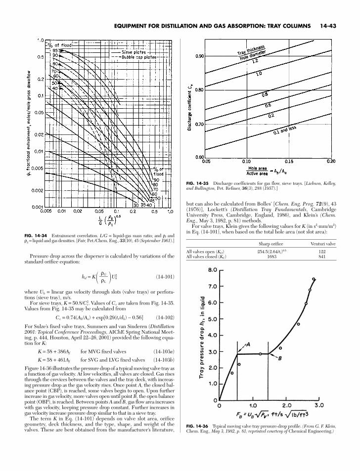
EQUIPMENT FOR DISTILLATION AND GAS ABSORPTION: TRAY COLUMNS 14-43

Pressure drop across the disperser is calculated by variations of thestandard orifice equation:

hd = K� U2h (14-101)

where Uh = linear gas velocity through slots (valve trays) or perfora-tions (sieve tray), m/s.

For sieve trays, K = 50.8/Cv2. Values of Cv are taken from Fig. 14-35.

Values from Fig. 14-35 may be calculated from

Cv = 0.74(Ah/Aa) + exp[0.29(tt/dh) − 0.56] (14-102)

For Sulze’s fixed valve trays, Summers and van Sinderen (Distillation2001: Topical Conference Proceedings, AIChE Spring National Meet-ing, p. 444, Houston, April 22–26, 2001) provided the following equa-tion for K:

K = 58 + 386Af for MVG fixed valves (14-103a)

K = 58 + 461Af for SVG and LVG fixed valves (14-103b)

Figure 14-36 illustrates the pressure drop of a typical moving valve tray asa function of gas velocity. At low velocities, all valves are closed. Gas risesthrough the crevices between the valves and the tray deck, with increas-ing pressure drop as the gas velocity rises. Once point A, the closed bal-ance point (CBP), is reached, some valves begin to open. Upon furtherincrease in gas velocity, more valves open until point B, the open balancepoint (OBP), is reached. Between points A and B, gas flow area increaseswith gas velocity, keeping pressure drop constant. Further increases ingas velocity increase pressure drop similar to that in a sieve tray.

The term K in Eq. (14-101) depends on valve slot area, orificegeometry, deck thickness, and the type, shape, and weight of thevalves. These are best obtained from the manufacturer’s literature,

ρG�ρL

but can also be calculated from Bolles’ [Chem. Eng. Prog. 72(9), 43(1976)], Lockett’s (Distillation Tray Fundamentals, CambridgeUniversity Press, Cambridge, England, 1986), and Klein’s (Chem.Eng., May 3, 1982, p. 81) methods.

For valve trays, Klein gives the following values for K (in s2⋅mm/m2)in Eq. (14-101), when based on the total hole area (not slot area):

Sharp orifice Venturi valve

All valves open (KO) 254.5(2.64/tt)0.5 122All valves closed (KC) 1683 841

FIG. 14-34 Entrainment correlation. L/G = liquid-gas mass ratio; and ρl andρg = liquid and gas densities. [Fair, Pet./Chem. Eng., 33(10), 45 (September 1961).]

FIG. 14-35 Discharge coefficients for gas flow, sieve trays. [Liebson, Kelley,and Bullington, Pet. Refiner, 36(3), 288 (1957).]

FIG. 14-36 Typical moving valve tray pressure-drop profile. (From G. F. Klein,Chem. Eng., May 3, 1982, p. 81; reprinted courtesy of Chemical Engineering.)

The velocity at which the valves start to open (point A) is given by

Uh,closed = 1.14[tv(Rvw/KC)(ρM/ρG)]0.5 (14-104)

where Uh, closed = hole area at point A, m/s; tv = valve thickness, mm; Rvw =ratio of valve weight with legs to valve weight without legs, given inTable 14-11; KC = orifice coefficient with all valves closed (see above),s2⋅mm/m2; ρM = valve metal density, kg/m3 (about 8000 kg/m3 forsteel); ρG = gas density, kg/m3.

The velocity at which all the valves are open Uh,open can be calcu-lated from

Uh,open = Uh,closed(KC/KO)0.5 (14-105)

Pressure drop through the aerated liquid [h′L, in Eq. (14-100)] iscalculated by

h′L = βhds (14-106)

where β = aeration factor, dimensionlesshds = calculated height of clear liquid, mm (dynamic seal)

The aeration factor β has been determined from Fig. 14-37 forvalve and sieve trays. For sieve trays, values of β in the figure may becalculated from

β = 0.0825 ln − 0.269 ln Fh + 1.679 (14-107)

where Lw = weir length, mFh = F-factor for flow through holes, Fh = UhρG

0.5, m/s (kg/m3)0.5

For sieve and valve trays,

hds = hw + how + 0.5hhg (14-108)

where hw = weir height, mmhow = height of crest over weir, mm clear liquidhhg = hydraulic gradient across tray, mm clear liquid

The value of weir crest how may be calculated from the Francis weirequation and its modifications for various weir types. For a segmentalweir and for height in millimeters of clear liquid,

how = 664� 2/3

(14-109)

where Q = liquid flow, m3/sLw = weir length, m

For serrated weirs,

how = 851� 0.4

(14-110)

where Q′ = liquid flow, m3/s per serrationθ = angle of serration, deg

For circular weirs,

how = 44,300� 0.704

(14-111)

where q = liquid flow, m3/sdw = weir diameter, mm

For most sieve and valve trays, the hydraulic gradient is small andcan be dropped from Eq. (14-108). Some calculation methods are

Q�dw

Q′�tan θ/2

Q�Lw

Q�Lw

available and are detailed in previous editions of this handbook. A ruleof thumb by the author is 17 mm/m (0.2 in/ft) of flow path length.This rule only applies in the liquid-loaded froth and emulsion regimes(QL >50 m3/hm or >5.5 gpm/in of outlet weir length). At lower liquidloads, the hydraulic gradient is less.

As noted, the weir crest how is calculated on an equivalent clear-liq-uid basis. A more realistic approach is to recognize that in general afroth or spray flows over the outlet weir (settling can occur upstreamof the weir if a large “calming zone” with no dispersers is used). Ben-nett et al. [AIChE J., 29, 434 (1983)] allowed for froth overflow in acomprehensive study of pressure drop across sieve trays; their corre-lation for residual pressure drop h′L in Eq. (14-100) is presented indetail in the previous (seventh) edition of this handbook, including aworked example. Although more difficult to use, the method of Ben-nett et al. was recommended when determination of pressure drop isof critical importance.

Example 11: Pressure Drop, Sieve Tray For the conditions ofExample 9, estimate the pressure drop for flow across one tray. The thickness ofthe tray metal is 2 mm. The superficial F-factor is 2.08 m/s(kg/m3)1/2.

Solution Equations (14-100), (14-106), and (14-107), where ht = hd +β(hw + how), are used. For FS = 2.08, FB = 2.32 and FH = 16.55. From Example 9, Lw =1.50 m and hw = 38 mm. For a liquid rate of 22,000 kg/hr, Q = 7.27(10−3) m3/s, andQ/Lw = 4.8(10−3). By Eq. (14-107) or Fig. 14-37, β = 0.48. From Eq. (14-102) orFig. 14-35, Cv= 0.75. Then, by Eq. (14-101), hd= 29.0 mm liquid. Using Eq. (14-109),how = 18.9 mm. Finally, ht = hd + β(hw + how) = 29.0 + 0.48(38 + 18.9) = 56.4 mmliquid.

When straight or serrated segmental weirs are used in a column ofcircular cross section, a correction may be needed for the distortedpattern of flow at the ends of the weirs, depending on liquid flow rate.The correction factor Fw from Fig. 14-38 is used directly in Eq. (14-109).Even when circular downcomers are utilized, they are often fed by theoverflow from a segmental weir.

Loss under Downcomer The head loss under the downcomerapron, as millimeters of liquid, may be estimated from

hda = 165.2� 2

(14-112)

where Q = volumetric flow of liquid, m3/s and Ada =most restrictive (min-imum) area of flow under the downcomer apron, m2. Equation (14-112)was derived from the orifice equation with an orifice coefficient of 0.6.Although the loss under the downcomer is small, the clearance is signif-icant from the aspect of tray stability and liquid distribution.

The term Ada should be taken as the most restrictive area for liquidflow in the downcomer outlet. Usually, this is the area under thedowncomer apron (i.e., the downcomer clearance times the length ofthe segmental downcomer), but not always. For instance, if an inletweir is used and the area between the segmental downcomer and theinlet weir is smaller than the area under the downcomer apron, thesmaller area should be used.

OTHER HYDRAULIC LIMITS

Weeping Weeping is liquid descending through the tray perfora-tions, short-circuiting the contact zone, which lowers tray efficiency.At the tray floor, liquid static head that acts to push liquid down theperforations is counteracted by the gas pressure drop that acts to holdthe liquid on the tray. When the static head overcomes the gas pres-sure drop, weeping occurs.

Some weeping usually takes place under all conditions due to slosh-ing and oscillation of the tray liquid. Generally, this weeping is too smallto appreciably affect tray efficiency. The weep point is the gas velocity atwhich weeping first becomes noticeable. At this point, little efficiency islost. As gas velocity is reduced below the weep point, the weep rateincreases. When the weep rate becomes large enough to significantlyreduce tray efficiency, the lower tray operating limit is reached.

The main factor that affects weeping is the fractional hole area. Thelarger it is, the smaller the gas pressure drop and the greater theweeping tendency. Larger liquid rates and taller outlet weirs increase

Q�Ada

14-44 EQUIPMENT FOR DISTILLATION, GAS ABSORPTION, PHASE DISPERSION, AND PHASE SEPARATION

TABLE 14-11 RVW Values for Eq. (14-104)

Valve type Sharp Venturi

Three-leg 1.23 1.29Four-leg 1.34 1.45Cages (no legs) 1.00 1.00

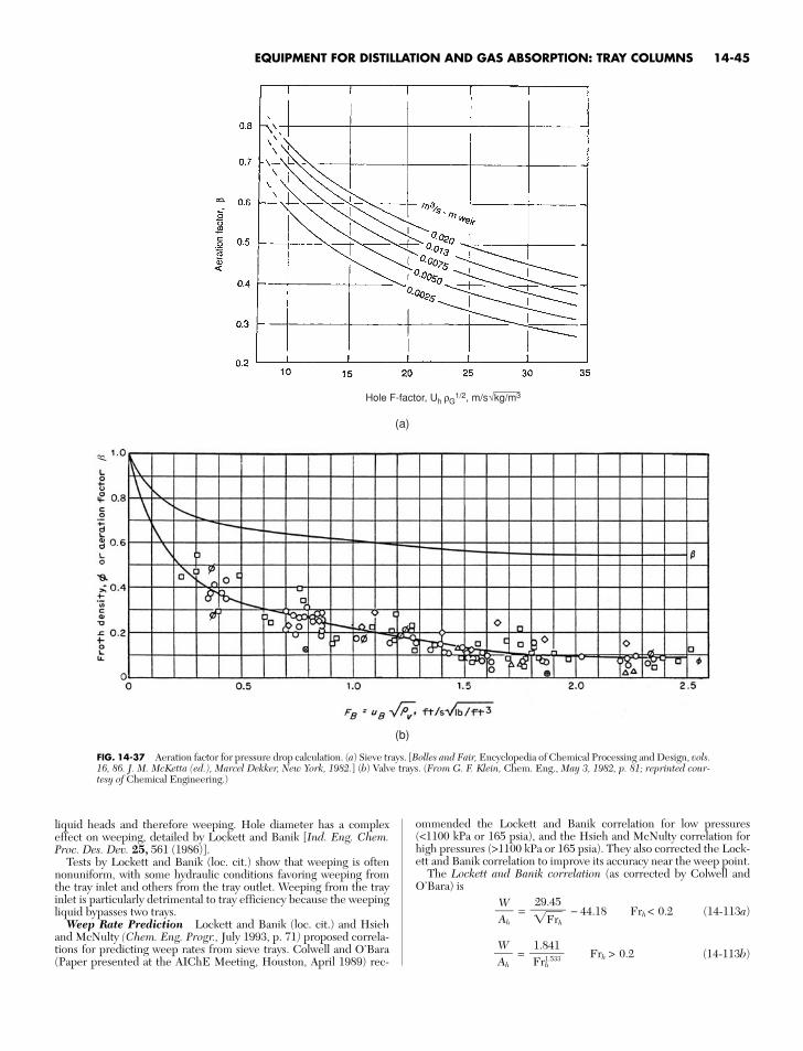
EQUIPMENT FOR DISTILLATION AND GAS ABSORPTION: TRAY COLUMNS 14-45

liquid heads and therefore weeping. Hole diameter has a complexeffect on weeping, detailed by Lockett and Banik [Ind. Eng. Chem.Proc. Des. Dev. 25, 561 (1986)].

Tests by Lockett and Banik (loc. cit.) show that weeping is oftennonuniform, with some hydraulic conditions favoring weeping fromthe tray inlet and others from the tray outlet. Weeping from the trayinlet is particularly detrimental to tray efficiency because the weepingliquid bypasses two trays.

Weep Rate Prediction Lockett and Banik (loc. cit.) and Hsiehand McNulty (Chem. Eng. Progr., July 1993, p. 71) proposed correla-tions for predicting weep rates from sieve trays. Colwell and O’Bara(Paper presented at the AIChE Meeting, Houston, April 1989) rec-

ommended the Lockett and Banik correlation for low pressures(<1100 kPa or 165 psia), and the Hsieh and McNulty correlation forhigh pressures (>1100 kPa or 165 psia). They also corrected the Lock-ett and Banik correlation to improve its accuracy near the weep point.

The Lockett and Banik correlation (as corrected by Colwell andO’Bara) is

= − 44.18 Frh< 0.2 (14-113a)

= Frh > 0.2 (14-113b)1.841�Frh

1.533

W�Ah

29.45��Frh�

W�Ah

Hole F-factor, Uh ρG1/2, m/s√kg/m3

(a)

(b)

FIG. 14-37 Aeration factor for pressure drop calculation. (a) Sieve trays. [Bolles and Fair, Encyclopedia of Chemical Processing and Design, vols.16, 86. J. M. McKetta (ed.), Marcel Dekker, New York, 1982.] (b) Valve trays. (From G. F. Klein, Chem. Eng., May 3, 1982, p. 81; reprinted cour-tesy of Chemical Engineering.)

where Frh = 0.373 (14-114)

Equations (14-113) and (14-114) use English units: W is the weeprate, gpm; Ah is the hole area, ft2; uh is the hole velocity, ft/s; and hc isthe clear liquid height, in. Colwell’s [Ind. Eng. Chem. Proc. Des. Dev.20(2), 298 (1981)] method below has been recommended for obtain-ing the clear liquid height hc in Eq. (14-114).

hc = φf{0.527� 2/3

+ hw} (14-115)

where φf is given by Eq. (14-119) and Cd is given by Eq. (14-116)

Cd = 0.61 + 0.08 �hh

fo

w

w� �

hh

fo

w

w� < 8.135f (14-116)

Cd = 1.06�1 + �hh

fo

w

w�

1.5�hh

fo

w

w� > 8.135

hfow = hf − hw (14-117)

where hf is given by Eq. (14-122). The froth density φf is calculatedfrom

η = 12.6Fr0.4 � 0.25

(14-118)

φf = (14-119)

Fr = 0.37 (14-120)

The term fw in Eq. (14-115) is the ratio of weep rate from the tray tothe total liquid flow entering the tray, calculated as follows:

fw = W/GPM (14-121)

Some trial and error is required in this calculation because the clearliquid height hc and the froth density φf depend on each other, and theweep fraction fw depends on the clear liquid height hc. Clear liquidheight is related to froth height and froth density by

hc = φfhf (14-122)

The terms in Eqs. (14-115) to (14-122) are in the English units and areexplained in the Nomenclature.

ρVu2B

��hc(ρL − ρV)

1�η + 1

AB�Ah

QL(1 − fw)��

Cdφf

ρV�ρL − ρV

u2h

�hc

With large-diameter trays and low liquid loads, a small ratio of W/Ah

corresponds to a large fractional weep. Under these conditions, theLockett and Banik correlation is inaccurate. The correlation is unsuit-able for trays with very small (<3-mm or �18�-in) holes. The correlationappears to fit most data points to an accuracy of ±15 to ±30 percent.The Hsieh and McNulty correlation (loc. cit.) is

�J*G� + m�J*L� = Cw (14-123)

where J*G = uh� �0.5

(14-124)

and

J∗L = � �

0.5(14-125)

Z = hc1.5/(12dH

0.5) (14-126)

The terms in Eqs. (14-123) to (14-126) are in English units and areexplained in the Nomenclature. For sieve trays, m = 1.94 and Cw = 0.79.Note that the constants are a slight revision of those presented in theoriginal paper (C. L. Hsieh, private communication, 1991). Clear liq-uid height is calculated from Colwell’s correlation [Eqs. (14-115) to(14-122)]. The Hsieh and McNulty correlation applies to trays with 9percent and larger fractional hole area. For trays with smaller holearea, Hsieh and McNulty expect the weeping rate to be smaller thanpredicted.

Weeping from Valve Trays An analysis of weeping from valvetrays [Bolles, Chem. Eng. Progs. 72(9), 43 (1976)] showed that in awell-designed valve tray, the weep point is below the gas load at whichthe valves open; and throughout the valve opening process, the oper-ating point remains above the weep point. In contrast, if the tray con-tains too many valves, or the valves are too light, excessive valveopening occurs before the gas pressure drop is high enough to counterweeping. In this case, weeping could be troublesome.

Weep point correlations for valve trays were presented by Bolles(loc. cit.) and by Klein (Chem. Eng., Sept. 17, 1984, p. 128). Hsieh andMcNulty (loc. cit.) gave a complex extension of their weep rate corre-lation to valve trays.

Dumping As gas velocity is lowered below the weep point, thefraction of liquid weeping increases until all the liquid fed to the trayweeps through the holes and none reaches the downcomer. This is thedump point, or the seal point. The dump point is well below the rangeof acceptable operation of distillation trays. Below the dump point,tray efficiency is slashed, and mass transfer is extremely poor. Opera-tion below the dump point can be accompanied by severe hydraulicinstability due to unsealing of downcomers.

Extensive studies on dumping were reported by Prince and Chan[Trans. Inst. Chem. Engr. 43, T49 (1965)]. The Chan and Prince

ρL��gZ(ρL − ρG)

W��448.83Ah

ρG��gZ(ρL − ρG)

14-46 EQUIPMENT FOR DISTILLATION, GAS ABSORPTION, PHASE DISPERSION, AND PHASE SEPARATION

FIG. 14-38 Correction for effective weir length. To convert gallons per minute to cubic meters per second, multiply by6.309 × 10−5; to convert feet to meters, multiply by 0.3048. [Bolles, Pet. Refiner, 25, 613 (1946).]

EQUIPMENT FOR DISTILLATION AND GAS ABSORPTION: TRAY COLUMNS 14-47

dump-point correlation was recommended and is presented in detailelsewhere (Kister, Distillation Design, McGraw-Hill, 1992). Alterna-tively, the dump point can be predicted by setting the weep rate equalto 100 percent of the liquid entering the tray in the appropriate weepcorrelation.

Turndown The turndown ratio is the ratio of the normal operat-ing (or design) gas throughput to the minimum allowable gas through-out. The minimum allowable throughput is usually set by excessiveweeping, while normal operating throughput is a safe margin awayfrom the relevant flooding limit.

Sieve and fixed valve trays have a poor turndown ratio (about 2 :1).Their turndown can be improved by blanking some rows of tray holes,which reduces the tendency to weep, but will also reduce the tray’s max-imum capacity. Turndown of moving valve trays is normally betweenabout 4 :1 to 5 :1. Special valve designs can achieve even better turn-down ratios, between 6 :1 and 10 :1, and even more. Turndown can alsobe enhanced by blanking strips (which require valve removal) or valveleg crimping. Sloley and Fleming (Chem. Eng. Progr., March 1994, p.39) stress that correct implementation of turndown enhancement iscentral to achieving a desired turndown. When poorly implemented,turndown may be restricted by poor vapor-liquid contact rather than byweeping.

Vapor Channeling All the correlations in this section assume anevenly distributed tray vapor. When the vapor preferentially channelsthrough a tray region, premature entrainment flood and excessiveentrainment take place due to a high vapor velocity in that region. Atthe same time, other regions become vapor-deficient and tend toweep, which lowers tray efficiency.

Work by Davies [Pet. Ref. 29(8), p. 93, and 29(9), p. 121 (1950)]based on bubble-cap tray studies suggests that the vapor pressure dropof the tray (the dry pressure drop) counteracts channeling. The higherthe dry tray pressure drop, the greater the tendency for vapor to spreaduniformly over the bubbling area. If the dry tray pressure drop is toosmall compared with the channeling potential, channeling prevails.

Perhaps the most common vapor channeling mechanism is vaporcrossflow channeling (VCFC, Fig. 14-39). The hydraulic gradient on thetray induces preferential vapor rise at the outlet and middle of the tray,and a vapor-deficient region near the tray inlet. The resulting high vaporvelocities near the tray outlet step up entrainment, while the low vaporvelocities near the tray inlet induce weeping. Interaction between adja-cent trays (Fig. 14-39) accelerates both the outlet entrainment and theinlet weeping. The net result is excessive entrainment and prematureflooding at the tray middle and outlet, simultaneous with weeping fromthe tray inlet, accompanied by a loss of efficiency and turndown.

VCFC takes place when the following four conditions exist simulta-neously [Kister, Larson, and Madsen, Chem. Eng. Progr., p. 86 (Nov.1992); Kister, The Chemical Engineer, 544, p. 18 (June 10, 1993)]:

1. Absolute pressure < 500 kPa (70 psia).2. High liquid rates [>50 m3/(m⋅h) or 6 gpm/in of outlet weir].3. High ratio (>2 :1) of flow path length to tray spacing.4. Low dry tray pressure drop. On sieve and fixed valve trays, this

means high (>11 percent) fractional hole area. On moving valve trays,this means venturi valves (smooth orifices) or long-legged valves (>15percent slot area). On all trays, the channeling tendency and severityescalate rapidly as the dry pressure drop diminishes (e.g., as fractionalhole area increases).

Hartman (Distillation 2001: Topical Conference Proceedings,AIChE Spring National Meeting, p. 108, Houston, Tex. (April 22–26,2001)] reports VCFC even with conventional valve trays (14 percentslot area) at very high ratio (3.6 :1) of flow path length to tray spacingand tray truss obstruction.

VCFC is usually avoided by limiting fractional hole areas, avoidingventuri valves, and using forward-push devices. Resitarits and Pap-pademos [Paper presented at the AIChE Annual Meeting, Reno, Nev.(November 2001)] cited tray inlet inactivity as a contributor to VCFC,and advocate inlet forward-push devices to counter it.

TRANSITION BETWEEN FLOW REGIMES

Froth-Spray Froth-spray transition has been investigated for sievetrays using a variety of techniques. The gradual nature of this transitionbred a multitude of criteria for defining it, and made its correlation diffi-cult. Excellent overviews were given by Lockett (Distillation Tray Fun-damentals, Cambridge University Press, Cambridge, England, 1986)and Prado, Johnson, and Fair [Chem. Eng. Progr. 83(3), p. 32 (1987)].Porter and Jenkins [I. Chem. E. Symp. Ser. 56, Summary Paper (1979)]presented a simple correlation for the froth-to-spray transition.

FLG = 0.0191 (14-127)

The terms of this equation are in English units and are explained in theNomenclature. This correlation is based on the premise that froth-to-spray transition occurs when the entrainment vs. liquid load relation-ship passes through a minimum (see “Entrainment”). Alternatively, itwas argued that the minimum represents a transition from the frothregime to a partially developed spray region (Kister, Pinczewski, andFell, Paper presented in the 90th National AIChE Meeting, Houston,April 1981). If this alternative argument is valid, then when the corre-lation predicts froth, it is highly unlikely that the column operates inthe spray regime; but when it predicts spray, the column may still beoperating in the froth regime. Recent entrainment studies by Ohe[Distillation 2005: Topical Conference Proceedings, AIChE SpringNational Meeting, p. 283, Atlanta (April 10–13, 2005)] argue that theentrainment minima represent minimum liquid residence times on thetray, and are unrelated to the froth-spray transition.

A second correlation is by Pinczeweski and Fell [Ind. Eng. Chem.Proc. Des. Dev. 21, p. 774 (1982)]

uB�ρG� = 2.25 � n

(14-128)

The terms of Eq. (14-128) are in English units and are explained inthe Nomenclature. The exponent n is calculated from Eq. (14-84).Equation (14-128) is based on transition data obtained from orificejetting measurements for the air-water system and on entrainmentminimum data for some hydrocarbon systems.

A third recent correlation by Johnson and Fair (loc. cit.) is

U*a = C1 ρG−0.50 ρL

0.692 σ0.06Af0.25�

0.05dh−0.1 (14-129)

where Ua* = gas velocity through active area at inversion, m/sρG = gas density, kg/m3

ρL = liquid density, kg/m3

σ = surface tension, mN/mAf = hole/active area ratio

q�Lw

QL�ρL��

100

NpAB�

Lw

FIG. 14-39 Vapor crossflow channeling. Note entrainment near the tray mid-dle and outlet, and weep near the tray inlet. (Kister, H. Z., K. F. Larson, and P.Madsen, Chem. Eng. Prog., Nov. 1992, p. 86; reproduced with permission.)

q/Lw = liquid flow, m3/(s⋅m) weirdh = hole diameter, mmC1 = 0.0583 for 25.4-mm overflow weirs

= 0.0568 for 50.4-mm overflow weirs= 0.0635 for 101.6-mm overflow weirs

Froth-Emulsion Froth-emulsion transition occurs [Hofhuis andZuiderweg, I. Chem. E. Symp. Ser. 56, p. 2, 2/1 (1979)] when the aer-ated mass begins to obey the Francis weir formula. Using this crite-rion, the latest version of this transition correlation is

FLG = 0.0208 (14-130)

The terms of this equation are in English units and are explained inthe Nomenclature; hc is calculated from the Hofhuis and Zuiderweg(loc. cit.) equation.

hc = 2.08�FLG p0.25

hw0.5 (14-131)

An inspection of the experimental data correlated shows that this,too, is a gradual transition, which occurs over a range of values ratherthan at a sharp point.

Valve Trays The amount of work reported thus far on valve trayregime transition is small and entirely based on air-water tests. Corre-lations proposed to date require the knowledge of liquid holdup attransition, which is generally not available, and are therefore of lim-ited application for commercial columns.

TRAY EFFICIENCY

DefinitionsOverall Column Efficiency This is the ratio of the number of

theoretical stages to the number of actual stages

EOC = Nt/Na (14-132)

Since tray efficiencies vary from one section to another, it is best toapply Eq. (14-132) separately for the rectifying and stripping sections.In practice, efficiency data and prediction methods are often toocrude to give a good breakdown between the efficiencies of differentsections, and so Eq. (14-132) is applied over the entire column.

Point Efficiency This is defined by Eq. (14-133) (Fig. 14-40a):

EOG = � point(14-133)

where y*n is the composition of vapor in equilibrium with the liquid atpoint n. The term yn is actual vapor composition at that point. The pointefficiency is the ratio of the change of composition at a point to thechange that would occur on a theoretical stage. As the vapor compositionat a given point cannot exceed the equilibrium composition, fractionalpoint efficiencies are always lower than 1. If there is a composition gra-dient on the tray, point efficiency will vary between points on the tray.

Murphree Tray Efficiency [Ind. Eng. Chem. 17, 747 (1925)]This is the same as point efficiency, except that it applies to the entiretray instead of to a single point (Fig. 14-40b):

EMV = � tray(14-134)

If both liquid and vapor are perfectly mixed, liquid and vapor compo-sitions on the tray are uniform, and the Murphree tray efficiency willcoincide with the point efficiency at any point on the tray. In practice,a concentration gradient exists in the liquid, and xn at the tray outlet islower than x′n on the tray (see Fig. 14-40b). This frequently lowers y*nrelative to yn, thus enhancing tray efficiency [Eq. (14-134)] comparedwith point efficiency. The value of y*n may even drop below yn. In thiscase, EMV exceeds 100 percent [Eq. (14-134)].

yn − yn−1�y*n − yn−1

yn − yn−1�y*n − yn−1

NpAB�

Lw

NpAB�Lwhc

Overall column efficiency can be calculated from the Murphreetray efficiency by using the relationship developed by Lewis [Ind.Eng. Chem. 28, 399 (1936)].

EOC = (14-135)

where λ = m (14-136)

Equation (14-135) is based on the assumption of constant molaroverflow and a constant value of EMV from tray to tray. It needs to beapplied separately to each section of the column (rectifying and strip-ping) because GM/LM, and therefore λ, varies from section to section.Where molar overflow or Murphree efficiencies vary throughout asection of column, the section needs to be divided into subsectionssmall enough to render the variations negligible.

The point and Murphree efficiency definitions above are expressedin terms of vapor concentrations. Analogous definitions can be madein terms of liquid concentrations. Further discussion is elsewhere(Lockett, Distillation Tray Fundamentals, Cambridge University,Press, Cambridge, England, 1986).

Fundamentals Figure 14-41 shows the sequence of steps forconverting phase resistances to a tray efficiency. Gas and liquid filmresistances are added to give the point efficiency. Had both vapor andliquid on the tray been perfectly mixed, the Murphree tray efficiencywould have equaled the point efficiency. Since the phases are not per-fectly mixed, a model of the vapor and liquid mixing patterns isneeded for converting point efficiency to tray efficiency. Liquid mix-ture patterns are plug flow, backmixing, and stagnant zones, whilevapor-mixing patterns are perfect mixing and plug flow.

Lewis (loc. cit.) was the first to derive quantitative relationshipsbetween the Murphree and the point efficiency. He derived threemixing cases, assuming plug flow of liquid in all. The Lewis cases givethe maximum achievable tray efficiency. In practice, efficiency islower due to liquid and vapor nonuniformities and liquid mixing.

Most tray efficiency models are based on Lewis case 1 with vaporperfectly mixed between trays. For case 1, Lewis derived the follow-ing relationship:

EMV,dry = (14-137)

The “dry” Murphree efficiency calculated thus far takes into accountthe vapor and liquid resistances and the vapor-liquid contact patterns,but is uncorrected for the effects of entrainment and weeping. Thiscorrection converts the dry efficiency to a “wet” or actual Murphreetray efficiency. Colburn [Eq. (14-98), under “Entrainment”] incorpo-rated the effect of entrainment on efficiency, assuming perfect mixingof liquid on the tray.

exp(λEOG) − 1��

λ

GM�LM

ln[1 + EMV(λ − 1)]��

ln λ

14-48 EQUIPMENT FOR DISTILLATION, GAS ABSORPTION, PHASE DISPERSION, AND PHASE SEPARATION

(a) (b)

FIG. 14-40 Point and Murphree efficiencies. (a) Point. (b) Murphree. (FromH. Z. Kister, Distillation Design, copyright © 1992 by McGraw-Hill; reprintedby permission.)

EQUIPMENT FOR DISTILLATION AND GAS ABSORPTION: TRAY COLUMNS 14-49

Factors Affecting Tray Efficiency Below is a summary based onthe industry’s experience. A detailed discussion of the fundamentals isfound in Lockett’s book (Distillation Tray Fundamentals, CambridgeUniversity Press, Cambridge, England, 1986). A detailed discussion ofthe reported experience, and the basis of statements made in this sectionare in Kister’s book (Distillation Design, McGraw-Hill, New York, 1992).

Errors in Vapor-Liquid Equilibrium (VLE) Errors in relativevolatility are the most underrated factor affecting tray efficiency. Figure14-42 shows the direct effect of the errors [Deibele and Brandt, Chem.Ing. Tech. 57(5), p. 439 (1985); Roy P. and G. K. Hobson, I. Chem. E.Symp. Ser. 104, p. A273 (1987)]. At very low relative volatilities(α < 1.2), small errors in VLE have a huge impact on tray efficiency.For instance, at α = 1.1, a −3 percent error gives a tray efficiency 40to 50 percent higher than its true value (Fig. 14-42). Since VLE errorsare seldom lower than ±2 to 3 percent, tray efficiencies of low-volatilitysystems become meaningless unless accompanied by VLE data. Like-wise, comparing efficiencies derived for a low-volatility system by differ-ent sources is misleading unless one is using identical VLE.

Figure 14-42 shows that errors in relative volatility are a problemonly at low relative volatilities; for α > 1.5 to 2.0, VLE errors have neg-ligible direct impact on tray efficiency.

Most efficiency data reported in the literature are obtained at totalreflux, and there are no indirect VLE effects. For measurements atfinite reflux ratios, the indirect effects below compound the directeffect of Fig. 14-42. Consider a case where αapparent < αtrue and test dataat a finite reflux are analyzed to calculate tray efficiency. Due to thevolatility difference Rmin,apparent > Rmin,true. Since the test was conductedat a fixed reflux flow rate, (R/Rmin)apparent < (R/Rmin)true. A calculationbased on the apparent R/Rmin will give more theoretical stages than acalculation based on the true R/Rmin. This means a higher apparentefficiency than the true value.

The indirect effects add to those of Fig. 14-42, widening the gapbetween true and apparent efficiency. The indirect effects exponen-tially escalate as minimum reflux is approached. Small errors in VLEor reflux ratio measurement (this includes column material balance aswell as reflux rate) alter R/Rmin. Near minimum reflux, even smallR/Rmin errors induce huge errors in the number of stages, and there-fore in tray efficiency. Efficiency data obtained near minimum refluxare therefore meaningless and potentially misleading.

Liquid Flow Patterns on Large Trays The most popular theo-retical models (below) postulate that liquid crosses the tray in plugflow with superimposed backmixing, and that the vapor is perfectlymixed. Increasing tray diameter promotes liquid plug flow and sup-presses backmixing.

The presence of stagnant zones on large-diameter distillation trays iswell established, but the associated efficiency loss is poorly understood;in some cases, significant efficiency losses, presumably due to stagnantzones, were reported [Weiler, Kirkpatrick, and Lockett, Chem. Eng.Progr. 77(1), 63 (1981)], while in other cases, no efficiency differencewas observed [Yanagi and Scott, Chem. Eng. Progr., 69(10), 75 (1973)].Several techniques are available for eliminating stagnant regions (seeKister, Distillation Design, McGraw-Hill, New York, 1992, for some),but their effectiveness for improving tray efficiency is uncertain.

Weir Height Taller weirs raise the liquid level on the tray in thefroth and emulsion regimes. This increases interfacial area and vaporcontact time, which should theoretically enhance efficiency. In thespray regime, weir height affects neither liquid level nor efficiency. Indistillation systems, the improvement of tray efficiency due to tallerweirs is small, often marginal.

Length of Liquid Flow Path Longer liquid flow paths enhancethe liquid-vapor contact time, the significance of liquid plug flow, andtherefore raise efficiency. Typically, doubling the flow path length

FIG. 14-41 Sequence of steps for theoretical prediction of tray efficiency. (From H. Z. Kister, Distil-lation Design, copyright © 1992 by McGraw-Hill; reprinted by permission.)

(such as going from two-pass to one-pass trays at a constant towerdiameter) raises tray efficiency by 5 to 15 percent.

Fractional Hole Area Efficiency increases with a reduction infractional hole area. Yanagi and Sakata [Ind. Eng. Chem. Proc. Des.Dev. 21, 712 (1982)] tests in commercial-scale towers show a 5 to 15percent increase in tray efficiency when fractional hole area was low-ered from 14 to 8 percent (Fig. 14-43).

Hole Diameter The jury is out on the effect of hole diameter ontray efficiency. There is, however, a consensus that the effect of holediameter on efficiency is small, often negligible.

Vapor-Liquid Loads and Reflux Ratio Vapor and liquid loads,as well as the reflux ratio, have a small effect on tray efficiency (Fig.14-43) as long as no capacity or hydraulic limits (flood, weep, chan-neling, etc.) are violated.

Viscosity, Relative Volatility Efficiency increases as liquid vis-cosity and relative volatility diminish. These effects are reflected inthe O’Connell correlation (below).

Surface Tension There is uncertainty regarding the effect of sur-face tension on tray efficiency. Often, it is difficult to divorce the sur-face tension effects from those of other physical properties.

Pressure Tray efficiency slightly increases with pressure (Fig.14-43), reflecting the rise of efficiency with a reduction in liquid vis-cosity and in relative volatility, which generally accompany a distillationpressure increase.

At pressures exceeding 10 to 20 bar (150 to 300 psia), and especiallyat high liquid rates, vapor entrainment into the downcomer liquidbecomes important, and tray efficiency decreases with furtherincreases in pressure [Zuiderweg, Int. Chem. Eng. 26(1), 1 (1986)].

Maldistribution Maldistribution can cause major efficiencyreduction in multipass trays (>two passes). Further discussion is givenunder “Number of Passes.”

OBTAINING TRAY EFFICIENCY

Efficiency prediction methods are listed here in decreasing order ofreliability.

Rigorous Testing Rigorous testing of a plant column is generallythe most reliable method of obtaining tray efficiency. Test procedurescan be found elsewhere (AIChE Equipment Testing ProceduresCommittee, AIChE Equipment Testing Procedure—Tray DistillationColumns, 2d ed., 1987; Kister, Distillation Operation, McGraw-Hill,New York, 1990).

Scale-up from an Existing Commercial Column As long asdata are for the same system under similar process conditions, load-ings, and operating regime, data obtained in one column directlyextend to another. Fractional hole area and the number of tray passeswill have a small but significant effect on efficiency, and any changes inthese parameters need to be allowed for during scale-up. The empiri-cal information in the section “Factors Affecting Tray Efficiency” canbe used to estimate the magnitude of the changes on efficiency.

Scale-up from Existing Commercial Column to DifferentProcess Conditions During scale-up, test data are analyzed bycomputer simulation. The number of theoretical stages is varied untilthe simulated product compositions and temperature profile matchthe test data. Tray efficiency is determined by the ratio of theoreticalstages to actual trays. In this procedure, errors in VLE are offset bycompensating errors in tray efficiency. For instance, if the relativevolatility calculated by the simulation is too high, fewer stages will beneeded to match the measured data, i.e., “apparent” tray efficiencywill be lower. Scale-up will be good as long as the VLE and efficiencyerrors continue to offset each other equally. This requires that processconditions (feed composition, feed temperature, reflux ratio, etc.)remain unchanged during scale-up.

When process conditions change, the VLE and efficiency errors nolonger offset each other equally. If the true relative volatility is higherthan simulated, then the scale-up will be conservative. If the true rel-ative volatility is lower than simulated, scale-up will be optimistic. Adetailed discussion is found in Kister, Distillation Design, McGraw-Hill, New York, 1992.

Experience Factors These are tabulations of efficiencies previ-ously measured for various systems. Tray efficiency is insensitive totray geometry (above), so in the absence of hydraulic anomalies andissues with VLE data, efficiencies measured in one tower are extensi-ble to others distilling the same system. A small allowance to variationsin tray geometry as discussed above is in order. Caution is requiredwith mixed aqueous-organic systems, where concentration may have amarked effect on physical properties, relative volatility, and efficiency.Table 14-12 shows typical tray efficiencies reported in the literature.

14-50 EQUIPMENT FOR DISTILLATION, GAS ABSORPTION, PHASE DISPERSION, AND PHASE SEPARATION

FIG. 14-42 Direct effect of errors in relative volatility on error in tray effi-ciency. (From H. Z. Kister, Distillation Design, copyright © 1992 by McGraw-Hill; reprinted by permission.)

FIG. 14-43 Efficiency reduction when fractional hole area is increased, alsoshowing little effect of vapor and liquid loads on efficiency in the normal oper-ating range (between excessive weeping and excessive entrainment). Also shownis the small increase in efficiency with pressure. FRI data, total reflux, DT = 1.2 m,S = 610 mm, hw = 50.8 mm, dH = 12.7 mm. (Reprinted with permission from T.Yanagi and M. Sakata, Ind. Eng. Chem. Proc. Des. Dev. 21, 712; copyright ©1982, American Chemical Society.)

EQUIPMENT FOR DISTILLATION AND GAS ABSORPTION: TRAY COLUMNS 14-51

Vital, Grossel and Olsen [Hydroc. Proc. 63, 11, p. 147 (1984)] andGarcia and Fair [Ind. Eng. Chem. Res. 39, p. 1809 (2000)] present anextensive tabulation of tray efficiency data collected from the pub-lished literature.

The GPSA Engineering Data Book (10th ed., Gas Processors Asso-ciation, 1987) and Kaes (Refinery Process Modeling—A PracticalGuide to Steady State Modeling of Petroleum Processes Using Com-mercial Simulators, Athens Printing Co., Athens, Ga., 2000) tabulatetypical efficiencies in gas plant and refinery columns, respectively.Pilling (Paper presented at the 4th Topical Conference on SeparationsScience and Technology, November 1999, available from SulzerChemtech, Tulsa, Okla.) tabulated more typical efficiencies. Similarinformation is often available from simulation guide manuals. Thequality and reliability of efficiencies from these sources vary and aregenerally lower than the reliability of actual measured data.

Scale-up from a Pilot- or Bench-Scale Column This is a verycommon scale-up. No reduction in efficiency on scale-up is expectedas long as several precautions are observed. These precautions, gener-ally relevant to pilot- or bench-scale columns, are spelled out with spe-cific reference to the Oldershaw column.

Scale-up from Oldershaw Columns One laboratory-scale devicethat found wide application in efficiency investigations is the Oldershawcolumn [Fig. 14-44, Oldershaw, Ind. Eng. Chem. Anal. Ed. 13, 265(1941)]. This column is available from a number of laboratory supplyhouses and can be constructed from glass for atmospheric operation orfrom metal for higher pressures. Typical column diameters are 25 to100 mm (1 to 4 in), with tray spacing the same as the column diameter.

Fair, Null, and Bolles [Ind. Eng. Chem. Process Des. Dev. 22, 53(1983)] found that efficiency measurements in Oldershaw columnsclosely approach the point efficiencies [Eq. (14-133)] measured in

TABLE 14-12 Representative Tray Efficiencies

Tray Column spacing, Pressure, Efficiency, % hole

Tray System diameter, ft in psia % (slot) area Ref.

Sieve Methanol-water 3.2 15.7 14.7 70–90 10.8 2Ethanol-water 2.5 14 14.7 75–85 10.4 1Methanol-water 3.2 15.7 14.7 90–100 4.8 2Ethylbenzene-styrene 2.6 19.7 1.9 70 12.3 5Benzene-toluene 1.5 15.7 14.7 60–75 8 10Methanol-n propanol-sec butanol 6.0 18 18 64* 6Mixed xylene + C8-C10 13.0 21 25 86* 4paraffins and naphthenes

Cyclohexane-n-heptane 4.0 24 5 60–70 14 924 80 14 9

4.0 24 5 70–80 8 824 90 8 8

Isobutane-n-butane 4.0 24 165 110 14 94.0 24 165 120 8 84.0 24 300 110 8 84.0 24 400 100 8 8

n-Heptane-toluene 1.5 15.7 14.7 60–75 8 10Methanol-water 2.0 13.6 14.7 68–72 10 11Isopropanol-water 2.0 13.6 14.7 59–63 11Toluene-methylcyclohexane 2.0 13.6 14.7 70–82 11Toluene stripping from water 4 24 14.7 31–42 8 13

Valve Methanol-water 3.2 15.7 14.7 70–80 14.7 2Ethanol-water 2.5 14 14.7 75–85 1Ethyl benzene-styrene 2.6 19.7 1.9 75–85 3Cyclohexane-n-heptane 4.0 24 24 70–96* 7Isobutane-n-butane 4.0 24 165 108–121* 7Cyclohexane-n-heptane 4.0 24 24 77–93† 14.7 12

5 57–86† 14.7 12Isobutane-n-butane 4.0 24 165 110–123† 14.7 12C3-C4 splitter 5.6 24 212 65–67‡ 12 14

References:1. Kirschbaum, Distillier-Rektifiziertechnik, 4th ed., Springer-Verlag, Berlin and Heidelberg, 1969.2. Kastanek and Standart, Sep. Sci. 2, 439 (1967).3. Billet and Raichle, Chem. Ing. Tech., 38, 825 (1966); 40, 377 (1968).4. AIChE Research Committee, Tray Efficiency in Distillation Columns, final report, University of Delaware, Newark, 1958.5. Billet R., IChemE., Symp. Ser. 32, p. 4:42 (1969).6. Mayfield et al., Ind. Eng. Chem., 44, 2238 (1952).7. Fractionation Research, Inc. “Report of Tests of Nutter Type B Float Valve Tray,” July 2, 1964 from Sulzer Chem Tech.8. Sakata and Yanagi, IChemE., Eng. Symp. Ser., no. 56, 3.2/21 (1979).9. Yanagi and Sakata, Ind. Eng. Chem. Process Des. Dec., 21, 712 (1982).

10. Zuiderweg and Van der Meer, Chem. Tech. (Leipzig), 24, 10 (1972).11. Korchinsky, Trans. I. Chem. E., 72, Part A, 472 (1994).12. Gliltsch, Inc. “Glitsch Ballast Trays,” Bulletin 159/160 (FRI Topical Report 15, 1958). Available from Koch-Glitsch LP,

Wichita, Kans.13. Kunesh et al., Paper presented at the AIChE Spring National Meeting, Atlanta, Ga., 1994.14. Remesat, Chuang, and Svrcek, Trans. I Chem. E., Vol. 83, Part A, p. 508, May 2005.Notes:*Rectangular Sulzer BDP valves.†Glitsch V-1 round valves (Koch-Glitsch).‡Two-pass trays, short path length.To convert feet to meters, multiply by 0.3048; to convert inches to centimeters, multiply by 2.54; and to convert psia to kilo-

pascals, multiply by 6.895.

commercial sieve-tray columns (Fig. 14-45) providing (1) the systemsbeing distilled are the same, (2) comparison is made at the same rela-tive approach to the flood point, (3) operation is at total reflux, and (4)a standard Oldershaw device is used in the laboratory experimentation.Fair et al. compared several systems, utilizing as large-scale informa-tion the published efficiency studies of Fractionation Research, Inc.(FRI).

A mixing model can be used to convert the Oldershaw point effi-ciencies to overall column efficiencies. This enhances the commercialcolumn efficiency estimates. A conservative approach suggested byFair et al. is to apply the Oldershaw column efficiency as the estimatefor the overall column efficiency of the commercial column, taking nocredit for the greater plug-flow character upon scale-up. The authorprefers this conservative approach, considering the poor reliability ofmixing models.

Previous work with Oldershaw columns [Ellis, Barker, and Con-tractor, Trans. Instn. Chem. Engnrs. 38, 21 (1960)], spells an addi-tional note of caution. Cellular (i.e., wall-supported) foam may form inpilot or Oldershaw columns, but is rare in commercial columns. For a

given system, higher Oldershaw column efficiencies were measuredunder cellular foam conditions than under froth conditions. For thisreason, Gerster [Chem. Eng. Progr. 59(3), 35 (1963)] warned thatwhen cellular foam can form, scale-up from an Oldershaw columnmay be dangerous. The conclusions presented by Fair et al. do notextend to Oldershaw columns operating in the cellular foam regime.Cellular foam can be identified by lower pilot column capacity com-pared to a standard mixture that is visualized not to form cellular foam.

Heat losses are a major issue in pilot and Oldershaw columns andcan lead to optimistic scale-up. Special precautions are needed tokeep these at a minimum. Vacuum jackets with viewing ports arecommonly used.

Uses of Oldershaw columns to less conventional systems and appli-cations were described by Fair, Reeves, and Seibert [Topical Confer-ence on Distillation, AIChE Spring Meeting, New Orleans, p. 27(March 10–14, 2002)]. The applications described include scale-up inthe absence of good VLE, steam stripping efficiencies, individualcomponent efficiencies in multicomponent distillation, determiningcomponent behavior in azeotropic separation, and foam testing.

Empirical Efficiency Prediction Two empirical correlationswhich have been the standard of the industry for distillation tray effi-ciency prediction are the Drickamer and Bradford, in Fig. 14-46[Trans. Am. Inst. Chem. Eng. 39, 319 (1943)] and a modification of itby O’Connell [Trans. Am. Inst. Chem. Eng. 42, 741 (1946)], in Fig.14-47. The Drickamer-Bradford plot correlates efficiency as a func-tion of liquid viscosity only, which makes it useful for petroleum cuts.O’Connell added the relative volatility to the x axis.

Lockett (Distillation Tray Fundamentals, Cambridge UniversityPress, Cambridge, England, 1986) noted some theoretical sense inO’Connell’s correlation. Higher viscosity usually implies lower diffu-sivity, and therefore greater liquid-phase resistance and lower effi-ciency. Higher relative volatility increases the significance of theliquid-phase resistance, thus reducing efficiency. Lockett expressesthe O’Connell plot in equation form:

EOC = 0.492(µLα)−0.245 (14-138)

14-52 EQUIPMENT FOR DISTILLATION, GAS ABSORPTION, PHASE DISPERSION, AND PHASE SEPARATION

FIG. 14-44 An Oldershaw column. (From H. Z. Kister, Distillation Design,copyright © 1992 by McGraw-Hill; reprinted by permission.)

FIG. 14-45 Overall column efficiency of 25-mm Oldershaw column comparedwith point efficiency of 1.22-m-diameter-sieve sieve-plate column of Fractiona-tion Research, Inc. System = cyclohexane-n-heptane. [Fair, Null, and Bolles,Ind. Eng. Chem. Process Des. Dev., 22, 53 (1982).]

FIG. 14-46 The Drickamer and Bradford tray efficiency correlation for refin-ery towers. To convert centipoise to pascal-seconds, multiply by 0.0001. [FromDrickamer and Bradford, Trans. Am. Inst. Chem. Eng. 39, 319 (1943).Reprinted courtesy of the AIChE.]

EQUIPMENT FOR DISTILLATION AND GAS ABSORPTION: PACKED COLUMNS 14-53

(The viscosity is in cP and EOC is fractional.) The volatility and viscos-ity are evaluated at the average arithmetic temperature between thecolumn top and bottom temperatures. The relative volatility isbetween the key components.

The O’Connell correlation was based on data for bubble-cap trays.For sieve and valve trays, its predictions are likely to be slightly con-servative.

Theoretical Efficiency Prediction Theoretical tray efficiencyprediction is based on the two-film theory and the sequence of stepsin Fig. 14-41. Almost all methods evolved from the AIChE model(AIChE Research Committee, Bubble Tray Design Manual, NewYork, 1958). This model was developed over 5 years in the late 1950sin three universities. Since then, several aspects of the AIChE modelhave been criticized, corrected, and modified. Reviews are given byLockett (Distillation Tray Fundamentals, Cambridge University Press,Cambridge, England, 1986) and Chan and Fair [Ind. Eng. Chem. Proc.

Des. Dev. 23, 814 (1984)]. An improved version of the AIChE model,which alleviated several of its shortcomings and updated its hydraulicand mass-transfer relationships, was produced by Chan and Fair.

The Chan and Fair correlation generally gave good predictionswhen tested against a wide data bank, but its authors also observedsome deviations. Its authors described it as “tentative until more databecome available.” The Chan and Fair correlation is considered themost reliable fundamental correlation for tray efficiency, but even thiscorrelation has been unable to rectify several theoretical and practicallimitations inherited from the AIChE correlation (see Kister, Distilla-tion Design, McGraw-Hill, New York, 1992). Recently, Garcia andFair (Ind. Eng. Chem. Res. 39, 1818, 2000) proposed a more funda-mental and accurate model that is also more complicated to apply.

The prime issue that appears to plague fundamental tray efficiencymethods is their tendency to predict efficiencies of 80 to 100 percentfor distillation columns larger than 1.2 m (4 ft) in diameter. In the realworld, most columns run closer to 60 percent efficiency. Cai and Chen(Distillation 2003: Topical Conference Proceedings, AIChE SpringNational Meeting, New Orleans, La., March 30–April 3, 2003) showthat published eddy diffusivity models, which are based on small-column work, severely underestimate liquid backmixing and overesti-mate plug flow in commercial-scale columns, leading to optimisticefficiency predictions. Which other limitations (if any) in the theoret-ical methods contribute to the mismatch, and to what degree, isunknown. For this reason, the author would not recommend any cur-rently published theoretical tray efficiency correlation for obtainingdesign efficiencies.

Example 12: Estimating Tray Efficiency For the column inExample 9, estimate the tray efficiency, given that at the relative volatility nearthe feed point is 1.3 and the viscosity is 0.25 cP.

Solution Table 14-12 presents measurements by Billet (loc. cit.) for ethyl-benzene-styrene under similar pressure with sieve and valve trays. The columndiameter and tray spacing in Billet’s tests were close to those in Example 9.Since both have single-pass trays, the flow path lengths are similar. The frac-tional hole area (14 percent in Example 9) is close to that in Table 14-12 (12.3percent for the tested sieve trays, 14 to 15 percent for standard valve trays). Sothe values in Table 14-12 should be directly applicable, that is, 70 to 85 percent.So a conservative estimate would be 70 percent. The actual efficiency should beabout 5 to 10 percent higher.

Alternatively, using Eq. (14-138) or Fig. 14-47, EOC = 0.492(0.25 × 1.3)−0.245 = 0.65or 65 percent. As stated, the O’Connell correlation tends to be slightly conserv-ative. This confirms that the 70 percent above will be a good estimate.

FIG. 14-47 O’Connell correlation for overall column efficiency Eoc for distilla-tion. To convert centipoises to pascal-seconds, multiply by 10−3. [O’Connell,Trans. Am. Inst. Chem. Eng., 42, 741 (1946).]

EQUIPMENT FOR DISTILLATION AND GAS ABSORPTION: PACKED COLUMNS

Packings are generally divided into three classes:1. Random or dumped packings (Figs. 14-48 and 14-49) are dis-

crete pieces of packing, of a specific geometric shape, that are“dumped” or randomly packed into the column shell.

2. Structured or systematically arranged packings (Fig. 14-50) arecrimped layers of corrugated sheets (usually) or wire mesh. Sectionsof these packings are stacked in the column.

3. Grids. These are also systematically arranged packings, butinstead of wire mesh or corrugated sheets, these use an open-latticestructure.

Random and structured packings are common in commercial prac-tice. The application of grids is limited primarily to heat-transfer andwash services and/or where a high fouling resistance is required. Gridsare discussed in detail elsewhere (Kister, Distillation Design,McGraw-Hill, New York, 1992).

Figure 14-51 is an illustrative cutaway of a packed tower, depictingtypical internals. This tower has a structured-packed top bed and arandom-packed bottom bed. Each bed rests on a support grid or plate.The lower bed has a holddown grid at its top to restrict packing uplift.Liquid to each of the beds is supplied by a liquid distributor. An inter-mediate distributor, termed a redistributor, is used to introduce feedand/or to remix liquid at regular height intervals. The intermediatedistributor in Fig. 14-51 is not self-collecting, so a chevron collector is

used to collect the liquid from the bed above. An internal pipe passesthis liquid to the distributor below. The collected liquid is mixed withthe fresh feed (not shown) before entering the distributor. Thereboiler return enters behind a baffle above the bottom sump.

As illustrated, the packing needs to be interrupted and a distributoradded at each point where a feed enters or a product leaves. A simpledistillation tower with a single feed will have a minimum of two beds,a rectifying bed and a stripping bed.

Packing Objectives The objective of any packing is to maximizeefficiency for a given capacity, at an economic cost. To achieve thesegoals, packings are shaped to

1. Maximize the specific surface area, i.e., the surface area per unitvolume. This maximizes vapor-liquid contact area, and, therefore,efficiency. A corollary is that efficiency generally increases as the ran-dom packing size is decreased or as the space between structuredpacking layers is decreased.

2. Spread the surface area uniformly. This improves vapor-liquidcontact, and, therefore, efficiency. For instance, a Raschig ring (Fig.14-48a) and a Pall® ring (Fig. 14-48c) of an identical size have identi-cal surface areas per unit volume, but the Pall® ring has a superiorspread of surface area and therefore gives much better efficiency.

3. Maximize the void space per unit column volume. This mini-mizes resistance to gas upflow, thereby enhancing packing capacity.

A corollary is that capacity increases with random packing size or withthe space between structured packing layers. Comparing with the firstobjective, a tradeoff exists; the ideal size of packing is a compromisebetween maximizing efficiency and maximizing capacity.

4. Minimize friction. This favors an open shape that has goodaerodynamic characteristics.

5. Minimize cost. Packing costs, as well as the requirements forpacking supports and column foundations, generally rise with theweight per unit volume of packing. A corollary is that packingsbecome cheaper as the size increases (random packing) and as thespace between layers increases (structured packing).

Random Packings Historically, there were three generations ofevolution in random packings. The first generation (1907 to the 1950s)produced two basic simple shapes—the Raschig ring and the Berl sad-dle (Fig. 14-48a, b) that became the ancestors of modern randompackings. These packings have been superseded by more modernpacking and are seldom used in modern distillation practice.

The second generation (late 1950s to the early 1970s) produced twopopular geometries—the Pall® ring, which evolved from the Raschigring, and the Intalox® saddle (Fig. 14-48c–f ), which evolved from theBerl saddle.

BASF developed the Pall® ring by cutting windows in the Raschigring and bending the window tongues inward. This opened up thering, lowering the aerodynamic resistance and dramatically enhanc-ing capacity. The bent tongues improved area distribution aroundthe particle, giving also better efficiency. These improvementsmade the first generation Raschig rings obsolete for distillation.

Berl saddles (ceramics) are still used due to their good breakageresistance.

The second-generation packings are still popular and extensivelyused in modern distillation practice. The third generation (the mid-1970s until present) has produced a multitude of popular geometries,most of which evolved from the Pall® ring and Intalox® saddle. Someare shown in Fig. 14-49. A more comprehensive description of thevarious packings is given elsewhere (Kister, Distillation Design,McGraw-Hill, New York, 1992).

The third generation of packing was a significant, yet not large,improvement over the second generation, so second-generation pack-ings are still commonly used.

Structured Packings Structured packings have been aroundsince as early as the 1940s. First-generation structured packings, suchas Panapak, never became popular, and are seldom used nowadays.

The second generation of structured packings began in the late1950s with high-efficiency wire-mesh packings such as Goodloe®,Hyperfil®, and the Sulzer® (wire-mesh) packings. By the early 1970s,these packings had made substantial inroads into vacuum distillation,where their low pressure drop per theoretical stage is a major advan-tage. In these services, they are extensively used today. Their highcost, high sensitivity to solids, and low capacity hindered their appli-cation outside vacuum distillation.

The corrugated-sheet packing, first introduced by Sulzer in the late1970s, started a third generation of structured packings. With a highcapacity, lower cost, and lower sensitivity to solids, while still retaining ahigh efficiency, these corrugated-sheet packings became competitivewith conventional internals, especially for revamps. The 1980s saw anaccelerated rise in popularity of structured packings, to the point oftheir becoming one of the most popular column internals in use today.

Corrugated structured packings are fabricated from thin, corrugated(crimped) metal sheets, arranged parallel to one another. The corru-gated sheets are assembled into an element (Figs. 14-50a, c and 14-51).The sheets in each element are arranged at a fixed angle to the vertical.Table 14-14 contains geometric data for several corrugated packings.

Geometry (Fig. 14-52) The crimp size defines the openingbetween adjacent corrugated layers. Smaller B, h, and S yield narroweropenings, more sheets (and, therefore, greater surface area) per unitvolume, and more efficient packing, but higher resistance to gas upflow,lower capacity, and enhanced sensitivity to plugging and fouling.

The corrugations spread gas and liquid flow through a single ele-ment in a series of parallel planes. To spread the gas and liquid uni-formly in all radial planes, adjacent elements are rotated so that sheetsof one element are at a fixed angle to the layer below (Fig. 14-51). Forgood spread, element height s is relatively short (typically 200 to 300mm, 8 to 12 in) and the angle of rotation is around 90°.

The surfaces of a few structured packings (especially those used inhighly fouling environments) are smooth. Most structured packingshave a roughened or enhanced surface that assists the lateral spread ofliquid, promotes film turbulence, and enhances the area available formass transfer. Texturing commonly employed is embossing and groov-ing (Fig. 14-50a, b).

The surfaces of most (but not all) structured packings contain holesthat serve as communication channels between the upper and lowersurfaces of each sheet. If the holes are too small, or nonexistent, bothsides of a sheet will be wet only at low liquid rates. At high liquid rates,sheeting or blanking will cause liquid to run down the top surface withlittle liquid wetting the bottom surface [Chen and Chuang, Hydroc.Proc. 68(2), 37 (1989)], which may lower efficiency. Usually, but notalways, the holes are circular (Fig. 14-50a, b), about 4 mm in diame-ter. Olujic et al. (Distillation 2003: Topical Conference Proceedings,p. 523, AIChE, 2003, Spring National Meeting, New Orleans, La.)showed that the hole diameter has a complex effect, strongly depen-dent on packing size, on both capacity and efficiency.

Inclination Angle In each element, corrugated sheets are mostcommonly inclined at about 45° to the vertical (typically indicated bythe letter ‘Y’ following the packing size). This angle is large enough forgood drainage of liquid, avoiding stagnant pockets and regions of liq-uid accumulation, and small enough to prevent gas from bypassing themetal surfaces. In some packings, the inclination angle to the verticalis steepened to 30° (typically indicated by the letter X following the

14-54 EQUIPMENT FOR DISTILLATION, GAS ABSORPTION, PHASE DISPERSION, AND PHASE SEPARATION

(a) (b)

(c) (d)

(e) (f)

FIG. 14-48 Common first- and second-generation random packings. (a)Raschig ring (metal, plastic, ceramic). (b) Berl saddle (ceramic). (c) Pall ring(metal). (d) Pall ring (plastic). (e) Intalox saddle (ceramic). (f ) Super Intalox sad-dle (plastic). (Parts d, f, courtesy of Koch-Glitsch LP.)

EQUIPMENT FOR DISTILLATION AND GAS ABSORPTION: PACKED COLUMNS 14-55

packing size). This improves drainage, and therefore capacity, but atthe expense of reduced gas-liquid contact, and therefore efficiency.

A recent development followed the realization that liquid drainagewas restricted at the element-to-element transition rather than insideelements (Lockett and Billingham, IChemE Symp. Ser. 152, London,2006). This means that the liquid accumulation leading to flood initi-ates at the transition region. A fourth generation of structured packingstarted, in which the main body of each element has layers inclined at45°, but the ends of each element are almost vertical to permitdrainage at this end region (Fig. 14-50d; but keep in mind that suc-cessive elements are rotated 90° rather than continuous, as shown inFig. 14-50d). These S-shaped or high-capacity packings offer greatercapacity compared to equivalent 45° inclined packings with efficiencythe same with some (Pilling and Haas, Topical Conference Proceed-ings, p. 132, AIChE Spring Meeting, New Orleans, March 10–14,2002; McNulty and Sommerfeldt in “Distillation: Horizons for theNew Millennium,” Topical Conference Proceedings, p. 89, AIChESpring Meeting, Houston, Tex., March 1999) and lower with others[Olujic et al., Chem. Eng. and Proc., 42, p. 55 (2003)].

PACKED-COLUMN FLOOD AND PRESSURE DROP

Pressure drop of a gas flowing upward through a packing countercur-rently to liquid flow is characterized graphically in Fig. 14-53. At verylow liquid rates, the effective open cross section of the packing is notappreciably different from that of dry packing, and pressure drop isdue to flow through a series of variable openings in the bed. Thus,pressure drop is proportional approximately to the square of the gas

velocity, as indicated in the region AB. At higher liquid rates, theeffective open cross section is smaller because of the presence ofliquid (region A′B′). The pressure drop is higher, but still propor-tional to the square of the gas velocity.

At higher gas rates, a portion of the energy of the gas stream isused to support an increasing quantity of liquid in the column. Forall liquid rates, a zone is reached where pressure drop is propor-tional to a gas flow rate to a power distinctly higher than 2; this zoneis called the loading zone. The increase in pressure drop is due to theliquid accumulation in the packing voids (region BC or B′C′)

As the liquid holdup increases, the effective orifice diameter maybecome so small that the liquid surface becomes continuous acrossthe cross section of the column. Column instability occurs concomi-tantly with a rising continuous-phase liquid body in the column. Pres-sure drop shoots up with only a slight change in gas rate (condition Cor C′). The phenomenon is called flooding and is analogous to entrain-ment flooding in a tray column.

Alternatively, a phase inversion occurs, and gas bubbles through theliquid. The column is not unstable and can be brought back to gas-phase continuous operation by merely reducing the gas rate. A stableoperating condition beyond flooding (region CD or C′D′) may formwith the liquid as the continuous phase and the gas as the dispersedphase [Lerner and Grove, Ind. Eng. Chem. 43, 216 (1951); Teller,Chem. Eng. 61(9), 168 (1954); Leung et al., Ind. Eng. Chem. Fund. 14(1), 63 (1975); Buchanan, Ind. Eng. Chem. Fund. 15 (1), 87 (1976)].

For total-reflux distillation in packed columns, regions of loadingand flooding are identified by their effects on mass-transfer efficiency,as shown in Fig. 14-54. Gas and liquid rate increase together, and a

FIG. 14-49 Common third-generation random packings. (a) Intalox metal tower packing(IMTP). (b) Cascade mini-ring (CMR) (plastic). (c) Nutter ring (metal). (d) Raschig Super-Ring(metal). (Parts a, b, courtesy of Koch-Glitsch LP; part c, courtesy of Sulzer Chemtech; part d,courtesy of Rashig AG.)

(b)(a)

(d)(c)

14-56 EQUIPMENT FOR DISTILLATION, GAS ABSORPTION, PHASE DISPERSION, AND PHASE SEPARATION

(a) (b)

(c) (d)

FIG. 14-50 Common structured packings. (a) A small element of MellapakTM showing embossed surface, holes, and corrugated-sheet arrangement. (b) Acloseup of the surface of FlexipacTM showing grooved surface and holes. (c) Fitting structured packing elements to a large-diameter tower. (d) Mellapak PlusTM, afourth-generation structured packing, showing a 45° inclination angle in the element and near-vertical inclination at the element-to-element transition. Note thatin the tower, the successive layers will be oriented 90° to each other as in part b. (Parts a, d, courtesy of Sulzer Chemtech; parts b, c, courtesy of Koch-Glitsch LP.)

point is reached at which liquid accumulates rapidly (point B) andeffective surface for mass transfer decreases rapidly.

Flood-Point Definition In 1966, Silvey and Keller [Chem. Eng.Progr. 62(1), 68 (1966)] listed 10 different flood point definitionsthat have been used by different literature sources. A later survey(Kister and Gill, Proceedings of Chemeca 92, p. 185-2, Canberra,Australia, 1992) listed twice that many. As Silvey and Keller pointedout, the existence of so many definitions puts into question what con-stitutes flooding in a packed tower, and at what gas rate it occurs.Symptoms used to identify flood in these definitions include appear-ance of liquid on top of the bed, excessive entrainment, a sharp rise

in pressure drop, a sharp rise in liquid holdup, and a sharp drop inefficiency. The survey of Kister and Gill suggests that most floodpoint definitions describe the point of flooding initiation (incipientflooding; point C or C′ on Figs. 14-53 and 14-54). The different incip-ient flooding definitions gave surprisingly little scatter of flood pointdata (for a given packing under similar operating conditions). It fol-lows that any definition describing flooding initiation should be satis-factory.

The author believes that due to the variations in the predominantsymptom with the system and the packing, the use of multiple symp-toms is most appropriate. The author prefers the following definition

by Fair and Bravo [Chem. Eng. Symp. Ser. 104, A183 (1987)]: “Aregion of rapidly increasing pressure drop with simultaneous loss ofmass transfer efficiency. Heavy entrainment is also recognized as asymptom of this region.” An almost identical definition was presentedearlier by Billet (Distillation Engineering, Chem. Publishing Co.,New York, 1979).

The maximum operational capacity or throughput (often alsoreferred to as maximum efficient capacity) is defined (Strigle, PackedTower Design and Applications, 2d ed., Gulf Publishing, Houston,Tex., 1994) as the “Maximum vapor rate that provides normal effi-ciency of a packing” (i.e., point B in Fig. 14-54). The MOC is clear-cutin Fig. 14-54. On the other hand, locating the MOC in other cases isdifficult and leaves a lot of room for subjectivity.

In most cases, [Kister and Gill, Chem. Eng. Progr. 87(2), 32 (1991)],the velocity at which MOC is reached is related to the flood pointvelocity by

uS,MOC = 0.95 uS,Fl (14-139)

Flood and Pressure Drop Prediction The first generalizedcorrelation of packed-column flood points was developed by Sher-wood, Shipley, and Holloway [Ind. Eng. Chem., 30, 768 (1938)] on thebasis of laboratory measurements primarily on the air-water systemwith random packing. Later work with air and liquids other than waterled to modifications of the Sherwood correlation, first by Leva [Chem.Eng. Progr. Symp. Ser., 50(1), 51 (1954)], who also introduced thepressure drop curves, and later in a series of papers by Eckert. Thegeneralized flooding–pressure drop chart by Eckert [Chem. Eng.Progr. 66(3), 39 (1970)], included in previous editions of this hand-book, was modified and simplified by Strigle (Packed Tower Designand Applications, 2d ed., Gulf Publishing, Houston, Tex., 1994) (Fig.14-55). It is often called the generalized pressure drop correlation(GPDC). The ordinate is a capacity parameter [Eq. (14-140)] relatedto the Souders-Brown coefficient used for tray columns.

CP = CSFp0.5ν0.05 = US�

0.50Fp

0.5ν0.05 (14-140)

where US = superficial gas velocity, ft/sρG, ρL = gas and liquid densities, lb/ft3 or kg/m3

ρG�ρL − ρG

Liquid Inlet

Liquid Distributor

Liquid Distributor

Column Sump

Packed Bed(Structured Packing)

Packed Bed(Random Packing)

FIG. 14-51 Illustrative cutaway of a packed tower, depicting an upper bed ofstructured packing and a lower bed of random packing. (Courtesy of SulzerChemtech.)

(b)(a)

FIG. 14-52 Crimp geometry in structured packings. (a) Flow channel crosssection. (b) Flow channel arrangement. (From J. R. Fair and J. L. Bravo, Chem.Eng. Progr., Jan. 1990, p. 19; reproduced courtesy of the American Institute ofChemical Engineers.)

FIG. 14-53 Pressure-drop characteristics of packed columns.

EQUIPMENT FOR DISTILLATION AND GAS ABSORPTION: PACKED COLUMNS 14-57

Fp = packing factor, ft−1

ν = kinematic viscosity of liquid, cSCS = C-factor, Eq. (14-77), based on tower superficial cross-

sectional area, ft/sCP = capacity factor, dimensional [units consisted with Eq.

(14-140) and its symbols]

The abscissa scale term is the same flow parameter used for tray(dimensionless):

FLG = � 0.5

(14-141)ρG�ρL

L�G

For structured packing, Kister and Gill [Chem. Eng. Symp. Ser. 128,A109 (1992)] noticed a much steeper rise of pressure drop with flowparameter than that predicted from Fig. 14-55, and presented a mod-ified chart (Fig. 14-56).

The GPDC charts in Figs. 14-55 and 14-56 do not contain specificflood curves. Both Strigle and Kister and Gill recommend calculatingthe flood point from the flood pressure drop, given by the Kister andGill equation

∆Pflood = 0.12Fp0.7 (14-142)

Equation (14-142) permits finding the pressure drop curve in Fig. 14-55or 14-56 at which incipient flooding occurs.

For low-capacity random packings, such as the small first-generationpackings and those smaller than 1-in diameter (Fp > 60 ft−1), calculatedflood pressure drops are well in excess of the upper pressure dropcurve in Fig. 14-55. For these packings only, the original Eckert floodcorrelation [Chem. Eng. Prog. 66(3), 39 (1970)] found in pre-1997 edi-tions of this handbook and other major distillation texts is suitable.

The packing factor Fp is empirically determined for each packingtype and size. Values of Fp, together with general dimensional data forindividual packings, are given for random packings in Table 14-13 (togo with Fig. 14-55) and for structured packings in Table 14-14 (to gowith Fig. 14-56).

Packing flood and pressure drop correlations should always be usedwith caution. Kister and Gill [Chem. Eng. Progr., 87(2), 32 (1991)]showed that deviations from the GPDC predictions tend to be system-atic and not random. To avoid regions in which the systematic deviationslead to poor prediction, they superimposed experimental data points foreach individual packing on the curves of the GPDC. Figure 14-57 is anexample. This method requires a single chart for each packing type andsize. It provides the highest possible accuracy as it interpolates measureddata and identifies uncertain regions. A set of charts is in Chapter 10 ofKister’s book (Distillation Design, McGraw-Hill, New York, 1992) with

14-58 EQUIPMENT FOR DISTILLATION, GAS ABSORPTION, PHASE DISPERSION, AND PHASE SEPARATION

FIG. 14-54 Efficiency characteristics of packed columns (total-reflux distillation.)

FIG. 14-55 Generalized pressure drop correlation of Eckert as modified by Strigle. To convert inches H2O to mm H2O, multiply by 83.31.(From Packed Tower Design and Applications by Ralph E. Strigle, Jr. Copyright © 1994 by Gulf Publishing Co., Houston, Texas. Used with per-mission. All rights reserved.)

EQUIPMENT FOR DISTILLATION AND GAS ABSORPTION: PACKED COLUMNS 14-59

updates in Kister, Lason, and Gill, Paper presented at the AIChE SpringNational Meeting, Houston, Tex., March 19–23, 1995; and in Kister,Scherffius, Afshar, and Abkar, in Distillation 2007: Topical ConferenceProceedings, 2007 AIChE Spring National Meeting, Houston, Texas.The latter reference also discusses correct and incorrect applications ofthose interpolation charts.

There are many alternative methods for flood and pressure dropprediction. The Billet and Schultes [IChemE Symp. Ser. 104, pp.A171 and B255 (1987)] and the Mackowiak (“Fluiddynamik vonKolonnen mit Modernen Füllkorpern und Packungen für Gas/Flus-sigkeitssysteme,” Otto Salle Verlag, Frankfurt am Main und VerlagSauerländer Aarau, Frankfurt am Main, 1991) correlations are ver-sions of the GPDC that take the liquid holdup into account. TheEiden and Bechtel correlation [IChemE Symp. Ser. 142, p. 757(1997)] is a version of the GPDC in which accuracy is improved byusing constants representative of packing shape instead of packingfactors. The Lockett and Billingham correlation (IChemE Symp.Ser. 152, p. 400, London, 2006) uses a Wallis correlation

CG0.5 + mCL

0.5 = CLG (14-143)

where CL = uL[ρL/(ρL − ρG)]0.5 (14-144)

and was shown to work well for high-surface-area (>400 m2/m3) struc-tured packings. Here CG is the gas C-factor, Eq. (14-77), based on thetower superficial cross-sectional area, and m and CLG are constants,available from the cited reference for some packing.

A drawback of most of these correlations (except that of Eiden andBechtel) is the unavailability of constants for many, often most, of themodern popular packings.

The above methods apply to nonfoaming systems. Foaming systemscan be handled either by applying additional derating (system) factors tothe flood correlation (see Table 14-9) or by limiting the calculated pres-sure drop to 0.25 in of water per foot of packing (Hausch, “DistillationTools for the Practicing Engineer,” Topical Conference Proceedings, p.119, AIChE Spring Meeting, New Orleans, March 10–14, 2002).

Pressure Drop The GPDC discussed above (Figs. 14-55 and14-56) and the Kister and Gill interpolation charts provide popularmethods for calculating packing pressure drops. An alternative popu-lar method that is particularly suitable for lower liquid loads was pre-sented by Robbins (below).

For gas flow through dry packings, pressure drop may be estimatedby use of an orifice equation. For irrigated packings, pressure drop

increases because of the presence of liquid, which effectivelydecreases the available cross section for gas flow (Fig. 14-53). In prin-ciple, there should be a method for correcting the dry pressure dropfor the presence of liquid. This approach was used by Leva [Chem.Eng. Progr. Symp. Ser. No. 10, 50, 51 (1954)]. A more recent methodby Robbins [Chem. Eng. Progr., p. 87 (May 1991)] utilizes the sameapproach and is described here. The total pressure drop is

∆Pt = ∆Pd + ∆PL (14-145)

where ∆Pt = total pressure drop, inches H2O per foot of packing∆Pd = dry pressure drop = C3Gf

210(C4Lf) (14-146)∆PL = pressure drop due to liquid presence

= 0.4[Lf /20,000]0.1[C3Gf210(C4Lf)]4 (14-147)

Gf = gas loading factor = 986Fs(Fpd/20)0.5 (14-148)Lf = liquid loading factor = L(62.4/ρL)(Fpd/20)0.5µL

0.1 (14-149)

The term Fpd is a dry packing factor, specific for a given packing typeand size. Values of Fpd are given in Tables 14-13 and 14-14. For operat-ing pressures above atmospheric, and for certain packing sizes, Lf andGf are calculated differently:

Gf = 986Fs(Fpd/20)0.5100.3ρG (14-150)

Lf = L(62.4/ρL)(Fpd/20)0.5µL0.2 Fpd > 200 (14-151a)

Lf = L(62.4/ρL)(20/Fpd)0.5µL0.1 Fpd < 15 (14-151b)

The Robbins equations require careful attention to dimensions. However,use of the equations has been simplified through the introduction of Fig.14-58. The terms Lf and Gf are evaluated, and the ∆PL is obtained directlyfrom the chart. Basic nomenclature for the Robbins method follows:

C3 = 7.4(10)−8

C4 = 2.7(10)−5

Fpd = dry packing factor, ft−1

Fs = superficial F-factor for gas, Utρg0.5, ft/s(lb/ft3)0.5

G = gas mass velocity, lb/hr⋅ft2

Gf = gas loading factor, lb/hr⋅ft2

L = liquid mass velocity, lb/hr⋅ft2

Lf = liquid loading factor, lb/hr⋅ft2

∆P = pressure drop, inches H2O/ft packing (× 83.3 =mm H2O/m packing)

FIG. 14-56 The Kister and Gill GPDC (SP) chart for structured packings only. Abscissa and ordinate same as in Fig.14-55. (From Kister, H. Z., and D. R. Gill, IChemE Symp. Ser. 128, p. A109, 1992. Reprinted courtesy of IChemE.)

TABLE 14-13 Characteristics of Random Packings

Packing factor, m−1

Size, Bed mm, or density,* Area, % Normal Dry

Name no. (#) kg/m3 m2/m3 voids Fp† Fpd

‡ Vendor

Metals

Pall rings 16 510 360 92 256 262 Various(also Flexi-rings, 25 325 205 94 183 174Ballast rings, P-rings) 38 208 130 95 131 91

50 198 105 96 89 7990 135 66 97 59 46

Metal Intalox (IMTP) 25 224 207 97 134 141 Koch-Glitsch[also I-rings, AHPP, 40 153 151 97 79 85 [Sulzer, Amistco,RSMR, MSR]§ 50 166 98 98 59 56 Rauschert, Montz]§

70 141 60 98 39 ––Nutter rings #0.7 177 226 98 — 128 Sulzer

#1 179 168 98 98 89#1.5 181 124 98 79 66#2 144 96 98 59 56#2.5 121 83 98 52 49#3.0 133 66 98 43 36

Raschig Super-ring #0.5 275 250 98 –– –– Raschig#0.7 185 175 98 –– ––#1 220 160 98 82 ––#1.5 170 115 98 59 ––#2 155 98 99 49 ––#3 150 80 98 36 ––

Cascade mini-rings #1 389 250 96 131 102 Koch-Glitsch(CMR) #1.5 285 190 96 95 —

#2 234 151 97 72 79#2.5 195 121 97 62 ––#3 160 103 98 46 43#4 125 71 98 33 32#5 108 50 98 26¶ ––

Fleximax #300 –– 141 98 85 –– Koch-Glitsch#400 –– 85 98 56 —

Jaeger Tripacks #1 223 118 96 85 –– Raschig(Top-Pak) #2 170 75 98 46 —VSP 25 352 206 98 105¶ –– Raschig

50 296 112 96 69 ––Ralu-rings 25 310 215 98 157¶ –– Raschig

38 260 135 97 92¶ ––50 200 105 98 66¶ ––

Hiflow 25 298 203 96 –– –– Rauschert50 175 92 98 52 —

Hy-Pak, K-Pak, #1 262 174 97 148 –– Koch-Glitsch,AIPR #1.5 180 118 98 95 –– Amistco

#2 161 92 98 85 ––#3 181 69 98 52 —

Raschig rings 19 1500 245 80 722 –– Various(1⁄16 in wall) 25 1140 185 86 472 492

50 590 95 92 187 22375 400 66 95 105 ––

CeramicsBerl saddles 6 900 900 60 — 2950 Various

13 865 465 62 790 90025 720 250 68 360 30838 640 150 71 215 15450 625 105 72 150 102

Intalox, Flexi-saddles, 6 864 984 65 — 2720 VariousTorus-saddles, Novalox 13 736 623 71 660 613

25 672 256 73 302 30850 608 118 76 131 12175 576 92 79 72 66

Raschig rings 6 960 710 62 –– 5250 Various13 880 370 64 1900 170525 670 190 74 587 49250 660 92 74 213 23075 590 62 75 121 ––

Pall ring 25 620 220 75 350 — Raschig38 540 164 78 180 —50 550 121 78 142 ––80 520 82 78 85¶ —

14-60

EQUIPMENT FOR DISTILLATION AND GAS ABSORPTION: PACKED COLUMNS 14-61

TABLE 14-13 Characteristics of Random Packings (Concluded )

Packing factor, m−1

Size, Bed mm, or density* Area, % Normal Dry

Name no. (#) kg/m3 m2/m3 voids Fp† Fpd

‡ Vendor

Ceramics

Hiflow rings 38 409 108 83 121 –– Rauschert50 405 89 82 95 ––70 333 52 86 49 —

Plastics

Pall rings 15 95 350 87 320 348 Various25 71 206 90 180 18040 70 131 91 131 13150 60 102 92 85 8290 43 85 95 56 39

Super Intalox, 25 83 207 90 131 131 VariousFlexi-saddles, 50 60 108 93 92 85Super-Torus, Novalox 75 48 89 96 59 46

Cascade mini-rings #1A 53 185 97 98 92 Koch-Glitsch(CMR) #2A 46 115 97 59 ––

#3A 40 74 98 39 33

Raschig Super-ring #0.6 62 205 96 105¶ — Raschig#2 55 100 96 49 —

Ralu-ring 15 80 320 94 230¶ — Raschig25 56 190 94 135 —38 65 150 95 80 —50 60 110 95 55 —90 40 75 96 38 —125 30 60 97 30¶ —

Snowflake — 51 92 97 43 — Koch-Glitsch

Nor-Pac 25 72 180 92 102 — NSW38 61 144 93 69 —50 53 102 94 46 —

Tri-Packs #1 67 158 93 53¶ — Raschig(Hacketten) #2 53 125 95 39¶ 43

Ralu-Flow #1 55 165 95 67¶ — Raschig#2 54 100 95 38¶ —

Hiflow 25 63 192 92 138 — Rauschert50 59 110 93 66 —90 34 65 97 30 —

Lanpac 90 67 148 93 46 — LantecImpac #3 83 213 91 49 —

Tellerettes 25 112 180 87 — 131 Ceilcote50 59 125 93 — —

*Values are approximate and may not be consistent. Actual number depends on wall thickness and material.†Packing factor Fp from Kister, Distillation Design, McGraw-Hill, 1992; Kister, Larson, and Gill, paper presented at the Houston

AIChE meeting, March 19–23, 1995; Strigle, Packed Tower Design and Applications, 2d ed., Gulf Publishing Co., Houston, Tex.,1994; Kister et al., in Distillation 2007. Topical Conference Proceedings, 2007 AIChE Spring National Meeting, Houston, Tex.

‡Dry packing factor Fpd from Robbins, Chem. Eng. Progr., 87(1), 19 (1990).§ The bracketed packings are similar to, but not the same as, the Koch-Glitsch IMTP. Some of them have holes that the

IMTP do not have, and others have sizes that are different and are made by different dies.¶Packing factor supplied by packing vendor. Vendors: Koch-Glitsch LLP, Wichita, Kansas; Raschig GmbH, Ludwigshafen/Rhein, Germany; Sulzer Chemtech Ltd., Win-

terthur, Switzerland; Rauschert Verfahrenstechnik GmbH, Steinwiesen, Germany; Amistco Separation Products Inc., Alvin,Texas; Julius Montz GmbH, Hilden, Germany; Ceilcote Co., Berea, Ohio; NSW Corp., Roanoke, Virginia; Lantec ProductsInc., Agoura Hills, California.

ρG = gas density, lb/ft3

ρL = liquid density, lb/ft3

µL = liquid viscosity, cP

The Robbins correlation applies near atmospheric pressure andunder vacuum, but is not suitable above 3 bar absolute. For high(>0.3) flow parameters [Eq. (14-141)], the correlation has only beentested with air-water data.

For flood and MOC predictions, Robbins recommends his pressuredrop method together with Eqs. (14-142) (flood) and (14-139) (MOC).

The GPDC and Robbins correlations are empirical. Fundamental cor-relations are also available. Most of these use the channel model, whichattributes the pressure drop to the resistance to flow in a multitude ofparallel channels. The channels may have bends, expansions, andcontractions. Popular application of this approach are the Rocha et al. cor-relation [Rocha, Bravo, and Fair, Ind. Eng. Chem. Res. 32, 641 (1993)] forstructured packing and the Mackowiak (“Fluiddynamik von Kolonnenmit Modernen Füllkorpern und Packungen für Gas/Flussigke-itssysteme,” Otto Salle Verlag, Frankfurt am Main und VerlagSauerländer Aarau, Frankfurt am Main, 1991) and Billet (Packed Column

Packing factor, m−1

Size Area, % Normal DryName or number m2/m3 voids* Fp

† Fpd‡ Vendor

4T 135 995T 90 99

5TX 90 99Super-Pak 250 250 98 55§ Raschig

350 350 98 70§

Ralu-Pak 250YC 250 98 66 RaschigRhombopac 4M 151 Kuhni

6M 230 599M 351

Max-Pak 0.5-in 229 98 39 RaschigMontz-Pak B1-125 125 97 Montz

B1-200 200B1-250 250 95 66B1-350 350 93

BSH-250¶ 250 95BSH-500¶ 500 91B1-250M 250 43B1-350M 350B1-500M 500

Wire Mesh

Sulzer AX 250 95 SulzerBX 492 90 69 (52.5)CY 700 85

BX Plus

Wire gauze BX 495 93 Koch-Glitsch

Montz-Pak A3-500 500 91 Montz

Goodloe 765 1010 96 Koch-Glitsch773 1920 95779 2640 92

Hyperfil 2300 2300 93.6 394/230§,|| 460 Knit Mesh 1900 1900 94.8 312/180§,||

1400 1400 96.0 180/131§,||

Ceramic

Flexeramic 28 260 66 131 Koch-Glitsch48 160 77 7988 100 86 49

Plastic

Mellapak 125Y 125 Sulzer250Y 250 72125X 125250X 250

Ralu-Pak 30/160 160 92 Raschig

Multifil plastics P1500 1500 88.5 Knit Mesh

Packing factor, m−1

Size Area, % Normal DryName or number m2/m3 voids* Fp

† Fpd‡ Vendor

Metals, corrugated sheets

Mellapak 125Y 125 99 33 Sulzer170Y 170 99 392Y 223 99 46

250Y 250 98 66350Y 350 98 75500Y 500 98 112750Y 750 97125X 125 99 16170X 170 99 202X 223 99 23

250X 250 98 26500X 500 98 82

Mellapak Plus 202Y 99 Sulzer252Y 250 98 39352Y 98452Y 350 98 69752Y 500 98 131

Flexipac 700Y 710 96 Koch-500Y 495 97 Glitsch1Y 420 98 98 (105)

350Y 350 981.6Y 290 98 59250Y 250 992Y 220 99 49 (36)

2.5Y 150 993.5Y 80 99 30 (15)4Y 55 99 23 (10.5)1X 420 98 52

350X 350 981.6X 290 98 33250X 250 992X 220 99 23

2.5X 150 993X 110 99 16

3.5X 80 994X 55 99

Flexipac 700 710 96 223 Koch-High-capacity 500Z 495 97 Glitsch

1Y 420 98 82350Y 350 981.6Y 290 99 56250Y 250 992Y 220 99 43

Intalox 1T 310 98 66 Koch-Glitsch1.5T 250 992T 215 99 563T 170 99 43

TABLE 14-14 Characteristics of Structured Packings

*% voids vary with material thickness and values may not be consistent.†Packing factors from Kister, Distillation Design, McGraw-Hill, 1992; Kister, Larson, and Gill, paper presented at the Houston AIChE Meeting, March 19–23, 1995;

and Kister et al., in Distillation 2007: Proceedings of Topical Conference, AIChE Spring Meeting, Houston, Tex., April 22–26, 2007.‡Dry packing factors from Robbins, Chem. Eng. Prog., p. 87, May 1991.§These packing factors supplied by the packing vendor.¶These are expanded metal packings.��First figure is for hydrocarbon service, second figure for aqueous service. Vendors: Sulzer Chemtech Ltd., Winterthur, Switzerland; Koch-Glitsch LLP, Wichita, Kansas; Raschig GmbH, Ludwigshafen/Rhein, Germany; Julius Montz

GmbH, Hilden, Germany; Knit Mesh/Enhanced Separation Technologies, Houston, Texas; Kuhni Ltd., Allschwil, Switzerland.

Analysis and Design, Ruhr University, Bochum, Germany, 1989)methods. Stichlmair et al. (Distillation Principles and Practices, Wiley,New York, 1998; Gas Sep. Purif. 3, March 1989, p. 19) present alter-native correlations using the particle model, that attributes packingpressure drop to friction losses due to drag of a particle. This is similarto the Ergun model for single-phase flow [Chem. Eng. Prog. 48(2), 89(1952)].

Example 13: Packed-Column Pressure Drop Air and water are flow-ing countercurrently through a bed of 2-inch metal Pall rings. The air mass velocityis 2.03 kg/s⋅m2 (1500 lbs/hr⋅ft2), and the liquid mass velocity is 12.20 kg/s⋅m2 (9000lbs/hr⋅ft2). Calculate the pressure drop by the generalized pressure drop (GPDC,Fig. 14-55) and the Robbins methods. Properties: ρG = 0.074 lbs/ft3; ρL = 62.4 lbs/ft3,µL = 1.0 cP, ν = 1.0 cS. The packing factor Fp = 27 ft−1. For Robbins, Fpd = 24 ft−1.The flow parameter FLG = L/G (ρG/ρL)0.5 = (9000/1500) (0.074/62.4)0.5 = 0.207. TheF-factor = Fs = UtρG

0.5 = G/(ρG0.53600) = 1500/[(0.074)0.5 (3600)] = 1.53 ft/s(lb/ft3)0.5.

14-62 EQUIPMENT FOR DISTILLATION, GAS ABSORPTION, PHASE DISPERSION, AND PHASE SEPARATION

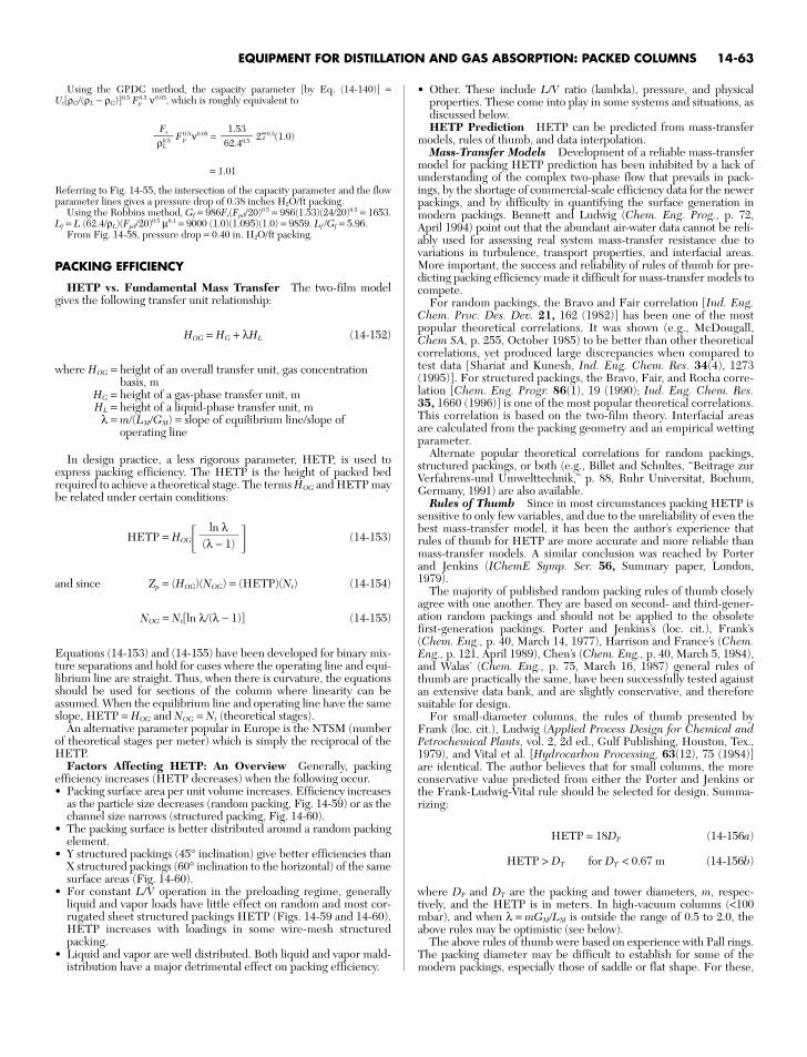
EQUIPMENT FOR DISTILLATION AND GAS ABSORPTION: PACKED COLUMNS 14-63

Using the GPDC method, the capacity parameter [by Eq. (14-140)] =Ut[ρG/(ρL − ρG)]0.5 Fp

0.5 ν0.05, which is roughly equivalent to

Fp0.5ν0.05 = 270.5(1.0)

= 1.01

Referring to Fig. 14-55, the intersection of the capacity parameter and the flowparameter lines gives a pressure drop of 0.38 inches H2O/ft packing.

Using the Robbins method, Gf = 986Fs(Fpd/20)0.5 = 986(1.53)(24/20)0.5 = 1653.Lf = L (62.4/ρL)(Fpd/20)0.5 µ0.1 = 9000 (1.0)(1.095)(1.0) = 9859. Lf /Gf = 5.96.

From Fig. 14-58, pressure drop = 0.40 in. H2O/ft packing.

PACKING EFFICIENCY

HETP vs. Fundamental Mass Transfer The two-film modelgives the following transfer unit relationship:

HOG = HG + λHL (14-152)

where HOG = height of an overall transfer unit, gas concentrationbasis, m

HG = height of a gas-phase transfer unit, mHL = height of a liquid-phase transfer unit, m

λ = m/(LM/GM) = slope of equilibrium line/slope ofoperating line

In design practice, a less rigorous parameter, HETP, is used toexpress packing efficiency. The HETP is the height of packed bedrequired to achieve a theoretical stage. The terms HOG and HETP maybe related under certain conditions:

HETP = HOG� � (14-153)

and since Zp = (HOG)(NOG) = (HETP)(Nt) (14-154)

NOG = Nt[ln λ/(λ − 1)] (14-155)

Equations (14-153) and (14-155) have been developed for binary mix-ture separations and hold for cases where the operating line and equi-librium line are straight. Thus, when there is curvature, the equationsshould be used for sections of the column where linearity can beassumed. When the equilibrium line and operating line have the sameslope, HETP = HOG and NOG = Nt (theoretical stages).

An alternative parameter popular in Europe is the NTSM (numberof theoretical stages per meter) which is simply the reciprocal of theHETP.

Factors Affecting HETP: An Overview Generally, packingefficiency increases (HETP decreases) when the following occur.• Packing surface area per unit volume increases. Efficiency increases

as the particle size decreases (random packing, Fig. 14-59) or as thechannel size narrows (structured packing, Fig. 14-60).

• The packing surface is better distributed around a random packingelement.

• Y structured packings (45° inclination) give better efficiencies thanX structured packings (60° inclination to the horizontal) of the samesurface areas (Fig. 14-60).

• For constant L/V operation in the preloading regime, generallyliquid and vapor loads have little effect on random and most cor-rugated sheet structured packings HETP (Figs. 14-59 and 14-60).HETP increases with loadings in some wire-mesh structuredpacking.

• Liquid and vapor are well distributed. Both liquid and vapor mald-istribution have a major detrimental effect on packing efficiency.

ln λ�(λ − 1)

1.53�62.40.5

Fs�ρL

0.5

• Other. These include L/V ratio (lambda), pressure, and physicalproperties. These come into play in some systems and situations, asdiscussed below.HETP Prediction HETP can be predicted from mass-transfer

models, rules of thumb, and data interpolation.Mass-Transfer Models Development of a reliable mass-transfer

model for packing HETP prediction has been inhibited by a lack ofunderstanding of the complex two-phase flow that prevails in pack-ings, by the shortage of commercial-scale efficiency data for the newerpackings, and by difficulty in quantifying the surface generation inmodern packings. Bennett and Ludwig (Chem. Eng. Prog., p. 72,April 1994) point out that the abundant air-water data cannot be reli-ably used for assessing real system mass-transfer resistance due tovariations in turbulence, transport properties, and interfacial areas.More important, the success and reliability of rules of thumb for pre-dicting packing efficiency made it difficult for mass-transfer models tocompete.

For random packings, the Bravo and Fair correlation [Ind. Eng.Chem. Proc. Des. Dev. 21, 162 (1982)] has been one of the mostpopular theoretical correlations. It was shown (e.g., McDougall,Chem SA, p. 255, October 1985) to be better than other theoreticalcorrelations, yet produced large discrepancies when compared totest data [Shariat and Kunesh, Ind. Eng. Chem. Res. 34(4), 1273(1995)]. For structured packings, the Bravo, Fair, and Rocha corre-lation [Chem. Eng. Progr. 86(1), 19 (1990); Ind. Eng. Chem. Res.35, 1660 (1996)] is one of the most popular theoretical correlations.This correlation is based on the two-film theory. Interfacial areasare calculated from the packing geometry and an empirical wettingparameter.

Alternate popular theoretical correlations for random packings,structured packings, or both (e.g., Billet and Schultes, “Beitrage zurVerfahrens-und Umwelttechnik,” p. 88, Ruhr Universitat, Bochum,Germany, 1991) are also available.

Rules of Thumb Since in most circumstances packing HETP issensitive to only few variables, and due to the unreliability of even thebest mass-transfer model, it has been the author’s experience thatrules of thumb for HETP are more accurate and more reliable thanmass-transfer models. A similar conclusion was reached by Porterand Jenkins (IChemE Symp. Ser. 56, Summary paper, London,1979).

The majority of published random packing rules of thumb closelyagree with one another. They are based on second- and third-gener-ation random packings and should not be applied to the obsoletefirst-generation packings. Porter and Jenkins’s (loc. cit.), Frank’s(Chem. Eng., p. 40, March 14, 1977), Harrison and France’s (Chem.Eng., p. 121, April 1989), Chen’s (Chem. Eng., p. 40, March 5, 1984),and Walas’ (Chem. Eng., p. 75, March 16, 1987) general rules ofthumb are practically the same, have been successfully tested againstan extensive data bank, and are slightly conservative, and thereforesuitable for design.

For small-diameter columns, the rules of thumb presented byFrank (loc. cit.), Ludwig (Applied Process Design for Chemical andPetrochemical Plants, vol. 2, 2d ed., Gulf Publishing, Houston, Tex.,1979), and Vital et al. [Hydrocarbon Processing, 63(12), 75 (1984)]are identical. The author believes that for small columns, the moreconservative value predicted from either the Porter and Jenkins orthe Frank-Ludwig-Vital rule should be selected for design. Summa-rizing:

HETP = 18DP (14-156a)

HETP > DT for DT < 0.67 m (14-156b)

where DP and DT are the packing and tower diameters, m, respec-tively, and the HETP is in meters. In high-vacuum columns (<100mbar), and when λ = mGM/LM is outside the range of 0.5 to 2.0, theabove rules may be optimistic (see below).

The above rules of thumb were based on experience with Pall rings.The packing diameter may be difficult to establish for some of themodern packings, especially those of saddle or flat shape. For these,

14-64 EQUIPMENT FOR DISTILLATION, GAS ABSORPTION, PHASE DISPERSION, AND PHASE SEPARATION

(a)

(b)

FIG. 14-57 Superimposing experimental pressure-drop data for a given packing generates a GPDC interpolationchart for this packing. (a) A random packing; chart is based on Eckert’s GPDC, Fig. 14-55. (b) A structured packing;chart is based on Kister and Gill’s GPDC (SP), Fig. 14-56. (From Kister, H. Z., Distillation Design, copyright ©McGraw-Hill, 1992; used with permission.)

Kister and Larson (in Schweitzer, Handbook of Separation Techniquesfor Chemical Engineers, 3d ed., McGraw-Hill, 1997) extendedEq. (14-156a) by expressing the packing diameter in terms of themore fundamental surface area per unit volume aP, m2/m3. For Pallrings, it can be shown that

aP = 5.2/DP (14-157)

and Eq. (14-156a) becomes

HETP = 93/aP (14-158)

EQUIPMENT FOR DISTILLATION AND GAS ABSORPTION: PACKED COLUMNS 14-65

FIG. 14-58 The Robbins generalized pressure-drop correlation. (From L. A.Robbins. Chem Eng. Progr., May 1991. p. 87, reprinted courtesy of the Ameri-can Institute of Chemical Engineers.)

100

3.5 inch (88.9 mm)

2 inch (50.8 mm)

5/8 inch (15.9 mm)

1 inch (25.4 mm)

90

80

70

60

50

40

30

20

10

00.0 0.4

0.50.0 1.0 1.5 2.0 2.5 3.0

0.8 1.2 2.82.42.01.60.0

0.4

0.8

1.2

HE

TP

, m

1.6

2.0

2.4

Fs, ft/s (lb/ft3)0.5

Fs, m/s (kg/m3)0.5

HE

TP

, in

FIG. 14-59 HETP values for four sizes of metal pall rings, vacuum operation. Cyclohexane/n-heptane system, total reflux, 35 kPa(5.0 psia). Column diameter = 1.2 m (4.0 ft). Bed height = 3.7 m (12 ft). Distributor = tubed drip pan, 100 streams/m2. [Adapted fromShariat and Kunesh, Ind. Eng. Chem. Res., 34, 1273 (1995). Reproduced with permission. Copyright © 1995 American ChemicalSociety.]

Harrison and France (loc. cit.) presented the only published rule ofthumb for structured packings efficiency as a function of packingcrimp. Kister and Larson reexpressed it in terms of the surface areaper unit volume to accommodate a wider range of packing geome-tries. The final expression is

HETP = 100CXY/ap + 0.10 (14-159)

Specific surface areas are listed in Tables 14-13 and 14-14.The above rules of thumb apply to organic and hydrocarbon sys-

tems, whose surface tensions are relatively low (σ < 25 mN/m). Forhigher surface tensions, the liquid does not adhere well to thepacking surfaces (underwetting), causing higher HETPs. In awater-rich system (σ = 70 mN/m or so) HETPs obtained from Eqs.(14-156), (14-158), and (14-159) need to be doubled. For interme-diate surface tension systems (some amines and glycols, whose sur-face tension at column conditions is 40 to 50 mN/m), HETPsobtained from Eqs. (14-156), (14-158), and (14-159) need to bemultiplied by 1.5.

For random packings, Eqs. (14-156) and (14-158) apply for pack-ings of 25-mm diameter and larger. For smaller packings, use of theap at 25-mm often gives a slightly conservative HETP estimate. Forstructured packing, CXY in Eq. (14-159) reflects the effect ofthe inclination angle (Fig. 14-60). CΞΨ = 1 for Y-type, S-type, or high-capacity packings, and CXY =1.45 for the larger (<300 m2/m3) X-typepackings. There are insufficient data to determine CXY for high spe-cific area X-type packings, but Fig. 14-60 suggests it is somewhatlower than 1.45.

Compared to experimental data, the above rules of thumb areslightly conservative. Since packing data are usually measured withperfect distribution, a slight conservative bias is necessary to extend

these data to the good, yet imperfect, distributors used in the realworld. For poor distributors, the above rules of thumb will usuallypredict well below the HETPs measured in the field.

Lockett (Chem. Eng. Progr., p. 60, January 1998) simplified thefundamental Bravo-Fair-Rocha correlation [Ind. Eng. Chem. Res. 35,p. 1660 (1996)] to derive an alternative rule of thumb for structuredpacking efficiency. This rule of thumb predicts HETPs under perfectdistribution conditions. Lockett recommends caution when applying

this rule of thumb for aqueous systems as it does not predict theeffects of underwetting (below).

Service-Oriented Rules of Thumb Strigle (Packed TowerDesign and Applications, 2d ed., Gulf Publishing, Houston, Tex.,1994) proposed a multitude of rules of thumb as a function of the ser-vice, column pressure, and physical properties. These rules are basedon the extensive experience of Strigle and the Norton Company (nowmerged with Koch-Glitsch LP).

14-66 EQUIPMENT FOR DISTILLATION, GAS ABSORPTION, PHASE DISPERSION, AND PHASE SEPARATION

FIG. 14-60 Effect of structured packing surface areas, loads, and inclination angle on packing efficiency. Effi-ciency expressed as number of theoretical stages per meter, the reciprocal of HETP. Sulzer data, chloroben-zene–ethylbenzene, 100 mbar, at total reflux; 250-mm-diameter test column. (Reprinted courtesy of SulzerChemtech.)

EQUIPMENT FOR DISTILLATION AND GAS ABSORPTION: PACKED COLUMNS 14-67

Data Interpolation Interpolation of experimental HETP data isthe most reliable means of obtaining design HETP values. This ishardly surprising in an area where our understanding of the theory isso poor that rules of thumb can do better than theoretical models. Theauthor believes that it is best to derive HETP from experimental data,and to check it against a rule of thumb.

Eckert [Chem. Eng. Progr. 59(5), 76 (1963)], Chen (Chem. Eng.p. 40, March 5, 1984), and Vital et al. [Hydroc. Proc. 63(12), 75(1984)] tabulated experimental HETP data for various random pack-ings. Kister (Distillation Design, McGraw-Hill, 1992) extended thesetabulations and included published HETP data and a detailed proce-dure for interpolating such HETP data. A prerequisite to any interpo-lation of packing data is thorough familiarity with the factors thataffect HETP. Overlooking any of the factors listed can easily lead topoor interpolation and grossly incorrect design. In particular, it isimperative to recognize that the quality of distribution in pilot towersis generally superior to the quality of distribution in commercial tow-ers.

Underwetting Laboratory- and pilot-scale distillation experi-ments with systems that exhibit large differences in surface tensionalong the column such as methanol-water showed a sharp drop in effi-ciency at the high-surface-tension end of the column [Ponter et al.,Trans. Instn. Chem. Engineers [London], 45, T345 (1967)]. Thereappeared to be a critical methanol composition below which perfor-mance deteriorated rapidly. The poor performance at the low-methanol-concentration end appeared independent of the type andsize of packing. Visual observations with disk columns attributed theseeffects to underwetting.

Underwetting is a packing surface phenomenon, which breaks upliquid film. The tendency of the liquid film to break (the degree ofwetting) is expressed by the contact angle (Fig. 14-61). A contactangle of 0° indicates perfect wetting; an angle of 180° indicates nowetting. Mersmann and Deixler [Chem. Ing. Tech. 58(1), 19 (1986)]provide a preliminary chart for estimating contact angles. The contactangle depends on both the surface and the liquid and is a strong func-tion of composition. In systems with large surface tension gradients,both contact angles and minimum wetting rates may vary rapidly withchanges of composition or surface tension. Extensive studies by Pon-ter et al. [loc. cit.; also, Ponter and Au-Yeung, Chem. Ing. Tech., 56(9),701 (1984)] showed that• Underwetting is most significant in aqueous-organic systems, and

tends to occur at the high-surface-tension (aqueous) end of thecomposition range. Liquid viscosity may also have an effect.

• Underwetting may be alleviated by changing the material and sur-face roughness of the packing.

• In systems susceptible to underwetting, column efficiency cansometimes (but not always) be improved by the addition of smallamounts of surfactants.Effect of Lambda Most packed-column efficiency testing has

been at total reflux. Some tests for both random and structured pack-ings [Billet, “Packed Towers Analysis and Design,” Ruhr University,Bochum, Germany, 1989; Meier, Hunkeler, and Stocker, IChemESymp. Ser. 56, 3.3/1 (1979); Eckert and Walter, Hydroc. Proc. 43(2),107 (1964)] suggest that efficiencies at finite reflux are similar to thoseat total reflux when lambda (λ = mGM/LM, which is the ratio of theslope of the equilibrium curve to the slope of the operating line)ranges between 0.5 and 2.0. This range is typical for most distillationsystems.

Koshy and Rukovena [Hydroc. Proc., 65(5), 64 (1986)], experi-menting with methanol-water and water-DMF using #25 IMTP pack-

ing in a pilot-scale column, observed a sharp efficiency drop when thegroup λ was greater than 2 or lower than 0.5. The efficiency loss esca-lated as λ deviated more from this range. Koshy and Rukovena recog-nized that surface tension gradients and underwetting may haveinfluenced some of their findings, but argue that the lambda effect isthe major cause for the efficiency differences observed in their tests.High-relative-volatility systems are those most likely to be affected byλ, because at low volatility, λ ranges from 0.5 to 2. Strigle (loc. cit.)quantified the lambda effect on HETP using the following equation:

Actual HETP/standard HETP = 1 + 0.278[ABS(ln λ)3] (14-160)

For 0.5 < λ < 2, Eq. (14-160) gives a ratio of less than 1.1; that is, it hasa little influence on HETP.

Pressure Generally, pressure has little effect on HETP of bothrandom and structured packing, at least above 100 mbar abs. At deepvacuum (<100 mbar), there are data to suggest that efficiencydecreases as pressure is lowered for random packings [Zelvinski,Titov, and Shalygin, Khim Tekhnol. Topl. Masel. 12(10) (1966)], butmost of these data can also be explained by poor wetting or maldistri-bution.

At high pressures (>15 to 20 bar), structured packing efficiencydiminishes as pressure is raised (Fitz, Shariat, and Spiegel, Paper pre-sented at the AIChE Spring National Meeting, Houston, Tex., March1995). Zuiderweg and Nutter [IChemE Symp. 128, A481 (1992)]report the same phenomenon, but to a much smaller extent, also inrandom packings. They explain the efficiency reduction at higherpressure by vapor backmixing. Nooijen et al. [IChemE Symp. Ser.142, 885 (1997)] concur, bringing a supporting case study in whichhigh-pressure distillation efficiency improved by splitting a packed bed.

With structured packings (only) FRI’s high-pressure (10 to 30 bar;flow parameters >0.25) distillation tests measured maxima, termedhumps in the HETP vs. load plot, typically at 65 to 90 percent of flood[Fitz, Shariat, and Kunesh, IChemE Symp. Ser. 142, 829 (1997); Caiet al., Trans IChemE 81, Part A, p. 85 (2003)]. These humps (Fig. 14-62)were not observed with lower pressure distillation (flow parameters<0.2) and appeared to intensify with higher pressure. The humps didnot always occur; some tests at different distributor positioning andwith larger packing showed no humps. Zuiderweg et al. [IChemESymp. Ser. 142, 865 (1997); Trans. IChemE 81, Part A, p. 85 (January2003)] and Nooijen et al. [IChemE Symp. Ser. 142, 885 (1997)]explain the humps by two-phase backmixing. At the high liquid loadsin high-pressure distillation, flow unevenness prematurely floodssome of the packing channels, carrying vapor bubbles downward andrecirculating liquid upward.

Physical Properties Data presented by a number of workers[e.g., Vital, Grossel, and Olsen, Hydroc. Proc. 63(12), 75 (1984)] sug-gest that, generally, random packing HETP is relatively insensitive tosystem properties for nonaqueous systems. A survey of data in Chapter

FIG. 14-61 Contact angles. (a) Acute, good wetting. (b) Obtuse, poor wetting.

FIG. 14-62 HETPo data as measured in the FRI column for the iC4/nC4 sys-tem at different pressures (bara), showing efficiency humps. (From J. L. Nooi-jen, K. A. Kusters, and J. J. B. Pek, IChemE Symp. Ser. 142, p. 885, 1997.Reprinted courtesy of IChemE.)

11 of Kister’s Distillation Design (McGraw-Hill, New York, 1992)leads to a similar conclusion for structured packings. For water-richsystems, packing HETPs tend to be much higher than for nonaqueoussystems due to their high lambda or surface underwetting, as dis-cussed above. High hydrogen concentrations (>30 percent or so in thegas) have also led to low packing efficiencies (Kister et al., Proc. 4thEthylene Producers Conference, AIChE, New Orleans, La., p. 283,1992), possibly due to the fast-moving hydrogen molecule draggingheavier molecules with it as it diffuses from a liquid film into thevapor.

Errors in VLE These affect packing HETP in the same way asthey affect tray efficiency. The discussions and derivation earlier inthis subsection apply equally to tray and packed towers.

Comparison of Various Packing Efficiencies for Absorptionand Stripping In past editions of this handbook, extensive data onabsorption/stripping systems were given. Emphasis was given to thefollowing systems:

Ammonia-air-water Liquid and gas phases contributing; chemical reaction contributing

Air-water Gas phase controllingSulfur dioxide-air-water Liquid and gas phase controllingCarbon dioxide-air-water Liquid phase controlling

The reader may refer to the data in the 5th edition. For the currentwork, emphasis will be given to one absorption system, carbon diox-ide-air-caustic.

Carbon Dioxide-Air-Caustic System The vendors of packingshave adopted this system as a “standard” for comparing the perfor-mance of different packing types and sizes for absorption/stripping.For tests, air containing 1.0 mol % CO2 is passed countercurrently toa circulating stream of sodium hydroxide solution. The initial concen-tration of NaOH in water is 1.0 N (4.0 wt %), and as the circulatingNaOH is converted to sodium carbonate it is necessary to make amass-transfer correction because of reduced mass-transfer rate in theliquid phase. The procedure has been described by Eckert et al. [Ind.Eng. Chem., 59(2), 41 (1967); Chem. Eng. Progr., 54(1), 790 (1958)].An overall coefficient is measured using gas-phase (CO2) concentra-tions:

KOGae =

(14-161)

The coefficients are usually corrected to a hydroxide conversion of 25percent at 24°C. For other conversions, Fig. 14-14 may be used.Reported values of KOGa for representative random packings are givenin Table 14-15. The effect of liquid rate on the coefficient is shown inFig. 14-63.

While the carbon dioxide/caustic test method has become accepted,one should use the results with caution. The chemical reaction masks

moles CO2 absorbed������time-bed volume-partial pressure CO2 driving force

the effect of physical absorption, and the relative values in the tablemay not hold for other cases, where much of the resistance to masstransfer is in the gas phase. Background on this combination of physi-cal and chemical absorption may be found earlier in the present sec-tion, under “Absorption with Chemical Reaction.”

14-68 EQUIPMENT FOR DISTILLATION, GAS ABSORPTION, PHASE DISPERSION, AND PHASE SEPARATION

TABLE 14-15 Overall Coefficients for Representative Packings

CO2-air-caustic system

Nominal size, Overall coefficient KOGa,mm kg⋅moles/(hr⋅m3⋅atm)

Ceramic raschig rings 25 37.050 26.1

Ceramic Intalox saddles 25 45.150 30.1

Metal pall rings 25 49.650 34.9

Metal Intalox saddles (IMTP®) 25 54.850 39.1

NOTE: Basis for reported values: CO2 concentration in inlet gas, 1.0 vol %; 1NNaOH solution in water, 25 percent NaOH conversion; temperature = 24°C;atmospheric pressure: gas rate = 1.264 kg/(s⋅m2); liquid rate = 6.78 kg/(s⋅m2).

SOURCE: Strigle, R. L., Packed Tower Design and Applications, 2d ed., GulfPubl. Co., Houston, 1994.

10

2

3

5

1

.2

0.1

.3

.4

.6

.8

500 1000100 2000 5000

Liquid rate, lbm/(hr•ft )

(a)K

Ga,

lb-m

oles

/hr,

ft3 ,

atm

sgnirllap''1 sgnirgihcsar''1

2

10

2

3

5

1

.2

.3

.4

.6

.8

500 1000 2000 5000

KG

a, lb

-mol

es/h

r, ft

3 , a

tm

sgnirllap''2 sgnirgihcsar''2

Liquid rate, lbm/(hr•ft )

(b)

2

0.1100

FIG. 14-63 Overall mass transfer coefficients for carbon dioxide absorbedfrom air by 1N caustic solution. (a) 1-in Pall rings and Raschig rings. (b) 2-in Pallrings and Raschig rings. Air rate = 0.61 kg/s⋅m2 (450 lb/hr⋅ft2). To convert fromlb/hr⋅ft2 to kg/s⋅m2, multiply by 0.00136. To convert from lb-moles/hr⋅ft3 atm tokg-moles/s⋅m3 atm, multiply by 0.0045. [Eckert et al., Chem. Eng. Progr., 54(1),70 (1958).]

EQUIPMENT FOR DISTILLATION AND GAS ABSORPTION: PACKED COLUMNS 14-69

Summary In the preloading regime, packing size, type, and dis-tribution affect HETP. With aqueous-organic systems, HETP may besensitive to underwetting and composition. A lambda value(λ = mGM/LM) outside the range of 0.5 to 2.0 causes HETP to rise, andso does a high hydrogen concentration. HETP of structured packingsmay also be affected by pressure (at high pressure), and vapor and liq-uid loads.

MALDISTRIBUTION AND ITS EFFECTSON PACKING EFFICIENCY

Modeling and Prediction Maldistribution may drasticallyreduce packing efficiency. HETP may increase by a factor as high as 2or 3 due to maldistribution. Shariat and Kunesh [Ind. Eng. Chem.Res., 34(4), 1273 (1995)] provide a good demonstration.

Early models [Mullins, Ind. Chem. Mfr., 33, 408 (1957); Manningand Cannon, Ind. Eng. Chem. 49(3), 347 (1957)] expressed the effectof liquid maldistribution on packing efficiency in terms of a simplechanneling model. A portion of the liquid bypasses the bed, undergo-ing negligible mass transfer, and then rejoins and contaminates therest of the liquid. Huber et al. [Chem. Ing. Tech. 39, 797 (1967);Chem. Eng. Sci. 21, 819 (1966)] and Zuiderweg et al. [IChemE Symp.Ser. 104, A217 (1987)] replaced the simple bypassing by variations inthe local L/V ratios. The overirrigated parts have a high L/V ratio, theunderirrigated parts a low L/V ratio. Regions with low L/V ratios expe-rience pinching, and, therefore, produce poor separation.

Huber et al. (loc. cit.) and Yuan and Spiegel [Chem. Ing. Tech. 54,774 (1982)] added lateral mixing to the model. Lateral deflection ofliquid by the packing particles tends to homogenize the liquid, thuscounteracting the channeling and pinching effect.

A third factor is the nonuniformity of the flow profile through thepacking. This nonuniformity was observed as far back as 1935 [Baker,Chilton, and Vernon, Trans. Instn. Chem. Engrs. 31, 296 (1935)] andwas first modeled by Cihla and Schmidt [Coll. Czech. Chem. Com-mun., 22, 896 (1957)]. Hoek (Ph.D. Thesis, The University of Delft,The Netherlands, 1983) combined all three factors into a singlemodel, leading to the zone-stage model below.

The Zone-Stage Model Zuiderweg et al. [IChemE Symp. Ser.104, A217, A233 (1987)] extended Hoek’s work combining the effectsof local L/V ratio, lateral mixing, and flow profile into a model describ-ing the effect of liquid maldistribution on packing efficiency. Thiswork was performed at Fractionation Research Inc. (FRI) and at TheUniversity of Delft in The Netherlands. The model postulates that, inthe absence of maldistribution, there is a “basic” (or “true” or “inher-ent”) HETP which is a function of the packing and the system only.This HETP can be inferred from data for small towers, in which lat-eral mixing is strong enough to offset any pinching. For a given initialliquid distribution, the model uses a diffusion-type equation to char-acterize the splitting and recombining of liquid streams in the hori-zontal and vertical directions. The mass transfer is then calculated byintegrating the liquid flow distribution at each elevation and the basicHETP. Kunesh et al. successfully applied the model to predict mea-sured effects of maldistribution on packing efficiency. However, thismodel is difficult to use and has not gained industrywide acceptance.

Empirical Prediction Moore and Rukovena [Chemical Plantsand Processing (European edition), p. 11, August 1987] proposed theempirical correlation in Fig. 14-64 for efficiency loss due to liquidmaldistribution in packed towers containing Pall® rings or MetalIntalox® packing. This correlation was shown to work well for severalcase studies (Fig. 14-64), is simple to use, and is valuable, at least as apreliminary guide.

To quantify the quality of liquid irrigation, the correlation uses thedistribution quality rating index. Typical indexes are 10 to 70 percentfor most standard commercial distributors, 75 to 90 percent for inter-mediate-quality distributors, and over 90 percent for high-performancedistributors. Moore and Rukovena present a method for calculating adistribution-quality rating index from distributor geometry. Theirmethod is described in detail in their paper as well as in Kister’s book(Distillation Operation, McGraw-Hill, New York, 1990).

Maximum Liquid Maldistribution Fraction fmax. To character-ize the sensitivity of packed beds to maldistribution, Lockett and

(a)

(b)

FIG. 14-64 Effect of irrigation quality on packing efficiency. (a) Case historiesdemonstrating efficiency enhancement with higher distribution quality rating. (b)Correlation of the effect of irrigation quality on packing efficiency. (From F. Mooreand F. Rukovena, Chemical Plants and Processing, Europe edition, Aug. 1987;reprinted courtesy of Chemical Plants and Processing.)

Billingham (Trans. IChemE. 80, Part A, p. 373, May 2002; Trans.IChemE. 81, Part A, p. 134, January 2003) modeled maldistribution astwo parallel columns, one receiving more liquid (1 + f )L, the otherreceiving less (1 − f )L. The vapor was assumed equally split (Fig. 14-65)

without lateral mixing. Because of the different L/V ratios, the overallseparation is less than is obtained at uniform distribution. A typicalcalculated result (Fig. 14-66) shows the effective number of stagesfrom the combined two-column system decreasing as the maldistribu-tion fraction f increases. Figure 14-66a shows that the decrease is min-imal in short beds (e.g., 10 theoretical stages) or when themaldistribution fraction is small. Figure 14-66a shows that there is alimiting fraction fmax which characterizes the maximum maldistribu-tion that still permits achieving the required separation. Physically, fmax

represents the maldistribution fraction at which one of the two paral-lel columns in the model becomes pinched. Figure 14-66b highlightsthe steep drop in packing efficiency upon the onset of this pinch.Billingham and Lockett derived the following equation for fmax in abinary system:

fmax = + − � � (14-162)

This equation can be used to calculate fmax directly without the needfor a parallel column model. Billingham and Lockett show that thevarious terms in Eq. (14-162) can be readily calculated from the out-put of a steady-state computer simulation. Multicomponent systemsare represented as binary mixtures, either by lumping componentstogether to form a binary mixture of pseudolight and pseudoheavycomponents, or by normalizing the mole fractions of the two key com-ponents. Once fmax is calculated, Billingham and Lockett propose thefollowing guidelines:• fmax <0.05, extremely sensitive to maldistribution. The required sep-

aration will probably not be achieved.• 0.05 < fmax <0.10, sensitive to maldistribution, but separation can

probably be achieved.• 0.10 < fmax <0.20, not particularly sensitive to maldistribution.• fmax >0.20 insensitive to maldistribution.Figure 14-66b shows that shortening the bed can increase fmax. Rela-tive volatility and L/V ratio also affect fmax. The bed length and L/Vratio can often be adjusted to render the bed less sensitive to maldis-tribution.

Implications of Maldistribution to Packing Design PracticeThese are discussed at length with extensive literature citation inKister’s book Distillation Operation, McGraw-Hill, New York, 1990.Below are the highlights:

x1 − xo�xN + 1 − xo

yN + 1 − yN��

yN − yo

x1 − xo�xN + 1 − xo

yN + 1 − yN��

yN − yo

1. Three factors appear to set the effect of maldistribution on effi-ciency:

a. Pinching. Regional changes in L/V ratio cause regional com-position pinches.

b. Lateral mixing. Packing particles deflect both liquid andvapor laterally. This promotes mixing of vapor and liquid and counter-acts the pinching effect.

c. Liquid nonuniformity. Liquid flows unevenly through thepacking and tends to concentrate at the wall.

2. At small tower-to-packing diameter ratios (DT/Dp < 10), the lat-eral mixing cancels out the pinching effect, and a greater degree ofmaldistribution can be tolerated without a serious efficiency loss. Athigh ratios (DT/Dp > 40), the lateral mixing becomes too small to offset

14-70 EQUIPMENT FOR DISTILLATION, GAS ABSORPTION, PHASE DISPERSION, AND PHASE SEPARATION

FIG. 14-65 Parallel-columns model. (From Lockett and Billingham, Trans.IChemE 80, Part A, p. 373, May 2002; reprinted courtesy of IChemE.)

FIG. 14-66 Loss of efficiency due to maldistribution as a function of maldis-tribution fraction f and the number of stages per bed for a given case study. (a)fmax and reduction in number of stages. (b) Showing larger efficiency loss athigher number of stages per bed and higher f. The steep drops indicate pinch-ing associated with fmax. (From Lockett and Billingham, Trans. IChemE 80, PartA, p. 373, May 2002; reprinted courtesy of IChemE.)

(a)

(b)

EQUIPMENT FOR DISTILLATION AND GAS ABSORPTION: PACKED COLUMNS 14-71

the pinching effect. The effects of maldistribution on efficiency aretherefore most severe in large-diameter columns and small-diameterpackings.

A good design practice is to seek a packing size that gives a DT/Dp

between 10 and 40. This is often impractical, and higher ratios arecommon. When DT/Dp exceeds 100, avoiding efficiency loss due tomaldistribution is difficult. Either ratios exceeding 100 should beavoided, or a special allowance should be made for loss of efficiencydue to maldistribution.

3. Wall flow effects become large when DT/Dp falls below about 10.Packing diameter should be selected such that DT/Dp exceeds 10.

4. Columns containing less than five theoretical stages per bed arerelatively insensitive to liquid maldistribution. With 10 or more stagesper bed, efficiency can be extremely sensitive to maldistribution(Strigle, Packed Tower Design and Applications, 2d ed., Gulf Publish-ing, Houston, Tex., 1994) (Fig. 14-66). Beds consisting of small pack-ings or structured packings, which develop more theoretical stagesper bed, are therefore more sensitive to maldistribution than equal-depth beds of larger packings. This is clearly demonstrated by FRI’sexperiments [Shariat and Kunesh, Ind. Eng. Chem. Res. 34(4), 1273(1995)]. Lockett and Billingham (Trans. IChemE, vol. 81, Part A, p.131, January 2003) concur with these comments when their procedure(above) indicates high sensitivity to maldistribution, but allow a highernumber of stages per bed when the sensitivity is low.

5. Maldistribution tends to be a greater problem at low liquid flowrates than at high liquid flow rates [Zuiderweg, Hoek, and Lahm, I.ChemE Symp. Ser. 104, A217 (1987)]. The tendency to pinch and tospread unevenly is generally higher at the lower liquid flow rates.

6. A packed column has reasonable tolerance for a uniform orsmooth variation in liquid distribution and for a variation that is totallyrandom (small-scale maldistribution). The impact of discontinuities orzonal flow (large-scale maldistribution) is much more severe [Zuider-weg et al., loc. cit.; Kunesh, Chem. Eng., p. 101, Dec. 7, 1987; Kunesh,Lahm, and Yanagi, Ind. Eng. Chem. Res. 26(9), 1845 (1987)]. This isso because the local pinching of small-scale maldistribution is evenedout by the lateral mixing, and therefore causes few ill effects. In con-trast, the lateral mixing either is powerless to rectify a large-scalemaldistribution or takes considerable bed length to do so (meanwhile,efficiency is lost).

Figure 14-67 shows HETPs measured in tests that simulate varioustypes of maldistribution in FRI’s 1.2-m column containing a 3.6-m bedof 1-in Pall® rings. The y axis is the ratio of measured HETP in themaldistribution tests to the HETP obtained with an excellent distrib-utor. Analogous measurements with structured packing were reportedby Fitz, King, and Kunesh [Trans. IChemE 77, Part A, p. 482 (1999)].Generally, the response of the structured packings resembled that ofthe Pall® rings, except as noted below.

Figure 14-67a shows virtually no loss of efficiency when a distribu-tor uniformly tilts, such that the ratio of highest to lowest flow is 1.25(i.e., a “1.25 tilt”). In contrast, an 11 percent chordal blank of a leveldistributor causes packing HETP to rise by 50 percent.

Figure 14-67b compares continuous tilts with ratios of highest tolowest flow of 1.25 and 1.5 to a situation where one-half of the distrib-utor passes 25 percent more liquid than the other half. The latter(“zonal”) situation causes a much greater rise in HETP than a “uni-form” maldistribution with twice as much variation from maximum tominimum.

Figure 14-67c shows results of tests in which flows from individualdistributor drip points were varied in a gaussian pattern (maxi-mum/mean = 2). When the pattern was randomly assigned, there wasno efficiency loss. When the variations above the mean were assignedto a “high zone,” and those below the mean to a “low zone,” HETProse by about 20 percent. With structured packing, both random andzonal maldistribution caused about the same loss of efficiency at thesame degree of maldistribution.

7. A packed bed appears to have a “natural distribution,” which isan inherent and stable property of the packings. An initial distributionwhich is better than natural will rapidly degrade to it, and one that isworse will finally achieve it, but sometimes at a slow rate. If the rate isextremely slow, recovery from a maldistributed pattern may not beobserved in practice (Zuiderweg et al., loc. cit.). Even though the

(a)

(b)

(c)

FIG. 14-67 Comparing the effects of “small-scale” and “large-scale” maldistri-bution on packing HETP. (a) Comparing the effect of a simulated continuoustilt (max/min flow ratio = 1.25) with the simulated effect of blanking a chordalarea equal to 11 percent of the tower area. (b) Comparing the effects of simu-lated continuous tilts (max/min flow ratios of 1.25 and 1.5) with the effects of asituation where one-half of the distributor passes 25 percent more liquid to theother half. (c) Comparing the effects of random maldistribution with those ofzonal maldistribution. (Reprinted with permission from J. G. Kunesh, L. Lahm,and T. Yahagi, Ind. Eng. Chem. Res., 26, p. 1845; copyright © 1987, AmericanChemical Society.)

volumetric distribution improves along the bed, the concentrationprofile could have already been damaged, and pinching occurs(Bonilla, Chem. Eng. Prog., p. 47, March 1993).

8. Liquid maldistribution lowers packing turndown. The 2-in Pallrings curve in Fig. 14-59 shows HETP rise upon reaching the distrib-utor turndown limit.

9. The major source of gas maldistribution is undersized gas inletand reboiler return nozzles, leading to the entry of high-velocity gasjets into the tower. These jets persist through low-pressure-dropdevices such as packings. Installing gas distributors and improving gasdistributor designs, even inlet baffles, have alleviated many of theseproblems. Vapor distribution is most troublesome in large-diametercolumns. Strigle (Packed Tower Design and Applications, 2d ed., GulfPublishing, Houston, Tex., 1994) recommends considering a gas dis-tributing device whenever the gas nozzle F-factor (FN = uNρG

0.5)exceeds 27 m/s (kg/m3)0.5, or the kinetic energy of the inlet gas exceeds8 times the pressure drop through the first foot of packing, or thepressure drop through the bed is less than 0.65 mbar/m. Gas maldis-tribution is best tackled at the source by paying attention to the gasinlet arrangements.

10. A poor initial liquid maldistribution may cause gas maldistribu-tion in the loading region, i.e., at high gas rates [Stoter, Olujic, and deGraauw, IChemE Symp. Ser. 128, A201 (1992); Kouri and Sohlo,IChemE Symp. Ser. 104, B193 (1987)]. At worst, initial liquid maldis-tribution may induce local flooding, which would channel the gas. Thesegregation tends to persist down the bed. Outside the loading region,the influence of the liquid flow on gas maldistribution is small or neg-ligible. Similarly, in high-gas-velocity situations, the liquid distributionpattern in the bottom structured packing layers is significantly influ-enced by a strongly maldistributed inlet gas flow [Olujic et al., Chem.Eng. and Processing, 43, 465 (2004)]. Duss [IChemE Symp. Ser. 152,418 (2006)] suggests that high liquid loads such as those experiencedin high-pressure distillation also increase the susceptibility to gasmaldistribution.

11. The effect of gas maldistribution on packing performance isriddled with unexplained mysteries. FRI’s (Cai, Paper presented atthe AIChE Annual Meeting, Reno, Nev., 2001) commercial-scaletests show little effect of gas maldistribution on both random andstructured packing efficiencies. Cai et al. (Trans IChemE 81, Part A,p. 85, 2003) distillation tests in a 1.2-m-diameter tower showed thatblocking the central 50 percent or the chordal 30 percent of the towercross-sectional area beneath a 1.7-m-tall bed of 250 m2/m3 structuredpacking had no effect on packing efficiency, pressure drop, or capac-ity. The blocking did not permit gas passage but allowed collection ofthe descending liquid. Simulator tests with similar blocking with pack-ing heights ranging from 0.8 to 2.4 m (Olujic et al., Chemical Engi-neering and Processing, 43, p. 465, 2004; Distillation 2003: TopicalConference Proceedings, AIChE Spring National Meeting, NewOrleans, La., AIChE, p. 567, 2003) differed, showing that a 50 percentchordal blank raised pressure drop, gave a poorer gas pattern, andprematurely loaded the packing. They explain the difference by theability of liquid to drain undisturbed from the gas in the blocked seg-ment in the FRI tests. Olujic et al. found that while gas maldistribu-tion generated by collectors and by central blockage of 50 percent ofthe cross-sectional areas was smoothed after two to three layers ofstructured packing, a chordal blockage of 30 to 50 percent of cross-sectional area generated maldistribution that penetrated deeply intothe bed.

12. Computational fluid dynamics (CFD) has been demonstratedeffective for analyzing the effects of gas inlet geometry on gas maldis-tribution in packed beds. Using CFD, Wehrli et al. (Trans. IChemE81, Part A, p. 116, January 2003) found that a very simple device suchas the V-baffle (Fig. 14-70) gives much better distribution than a barenozzle, while a more sophisticated vane device such as a Schoepen-toeter (Fig. 14-71c) is even better. Implications of the gas inlet geom-etry to gas distribution in refinery vacuum towers was studied byVaidyanathan et al. (Distillation 2001, Topical Conference Proceed-ings, AIChE Spring National Meeting, Houston, Tex., p. 287, April22–26, 2001); Paladino et al. (Distillation 2003: Topical ConferenceProceedings, AIChE Spring National Meeting, New Orleans, La.,p. 241, 2003); Torres et al. (ibid., p. 284); Waintraub et al. (Distillation

2005: Topical Conference Proceedings, AIChE Spring NationalMeeting, Atlanta, Ga., p. 79, 2005); and Wehrli et al. (IChemE Symp.Ser 152, London, 2006). Vaidyanathan et al. and Torres et al. exam-ined the effect of the geometry of a chimney tray (e.g., Fig. 14-72)above the inlet on gas distribution and liquid entrainment. Paladinoet al. demonstrated that the presence of liquid in the feed affects thegas velocity profile, and must be accounted for in modeling. Paladinoet al. and Waintraub et al. used their two-fluid model to study thevelocity distributions and entrainment generated by different designsof vapor horns (e.g., Fig. 14-71). Wehrli et al. produced pilot-scaledata simulating a vacuum tower inlet, which can be used in CFDmodel validation. Ali et al. (Trans. IChemE, vol. 81, Part A, p. 108,January 2003) found that the gas velocity profile obtained using acommercial CFD package compared well to those measured in a 1.4-m simulator equipped with structured packing together with com-mercial distributors and collectors. Their CFD model effectivelypointed them to a collector design that minimizes gas maldistribution.

PACKED-TOWER SCALE-UP

Diameter For random packings there are many reports [Billet,Distillation Engineering, Chem Publishing Co., New York, 1979;Chen, Chem. Eng., p. 40, March 5, 1984; Zuiderweg, Hoek, andLahm, IChemE. Symp. Ser. 104, A217 (1987)] of an increase inHETP with column diameter. Billet and Mackowiak’s (Billet, PackedColumn Analysis and Design, Ruhr University, Bochum, Germany,1989) scale-up chart for Pall® rings implies that efficiency decreases ascolumn diameter increases.

Practically all sources explain the increase of HETP with columndiameter in terms of enhanced maldistribution or issues with thescale-up procedure. Lab-scale and pilot columns seldom operate atcolumn-to-packing diameter ratios (DT/Dp) larger than 20; underthese conditions, lateral mixing effectively offsets loss of efficiencydue to maldistribution pinch. In contrast, industrial-scale columnsusually operate at DT/Dp ratios of 30 to 100; under these conditions,lateral mixing is far less effective for offsetting maldistribution pinch.

To increase DT/Dp, it may appear attractive to perform the bench-scaletests using a smaller packing size than will be used in the prototype.Deibele, Goedecke, and Schoenmaker [IChemE Symp. Ser. 142, 1021(1997)], Goedecke and Alig (Paper presented at the AIChE SpringNational Meeting, Atlanta, Ga., April 1994), and Gann et al. [Chem. Ing.Tech., 64(1), 6 (1992)] studied the feasibility of scaling up from 50- to 75-mm-diameter packed columns directly to industrial columns. Deibeleet al. and Gann et al. provide an extensive list of factors that can affectthis scale-up, including test mixture, packing pretreatment, columnstructure, packing installation, snug fit at the wall, column insulation andheat losses, vacuum tightness, measurement and control, liquid distribu-tion, reflux subcooling, prewetting, sampling, analysis, adjusting thenumber of stages to avoid pinches and analysis issues, evaluation proce-dure, and more. Data from laboratory columns can be particularly sensi-tive to some of these factors. Goedecke and Alig show that for wire-meshstructured packing, bench-scale efficiency tends to be better than large-column efficiency, while for corrugated-sheets structured packing, theconverse occurs, possibly due to excessive wall flow. For some packings,variation of efficiency with loads at bench scale completely differs fromits variation in larger columns. For one structured packing, Kuhni Rom-bopak 9M, there was little load effect and there was good consistencybetween data obtained from different sources—at least for one test mix-ture. Deibele et al. present an excellent set of practical guidelines toimprove scale-up reliability. So, it appears that great caution is requiredfor packing data scale-up from bench-scale columns.

Height Experimental data for random packings show that HETPslightly increases with bed depth [Billet, Distillation Engineering,Chemical Publishing Co., New York, 1979; “Packed Tower Analysisand Design,” Ruhr University, Bochum, Germany, 1989; Eckert andWalter, Hydrocarbon Processing, 43(2), 107 (1964)].

For structured packing, some tests with Mellapak 250Y [Meier,Hunkeler, and Stöcker, IChemE Symp. Ser. 56, p. 3, 3/1 (1979)]showed no effect of bed height on packing efficiency, while others(Cai et al., Trans IChemE, vol. 81, Part A, p. 89, January 2003) didshow a significant effect.

14-72 EQUIPMENT FOR DISTILLATION, GAS ABSORPTION, PHASE DISPERSION, AND PHASE SEPARATION

EQUIPMENT FOR DISTILLATION AND GAS ABSORPTION: PACKED COLUMNS 14-73

The effect of bed depth on packing HETP is attributed to liquidmaldistribution. Zuiderweg et al. [IChemE. Symp. Ser. 104, A217(1987)] suggest that the uneven irrigation generates an uneven con-centration profile and localized pinching near the bottom of the beds.The tests by Martin, Bravo, and Fair (Paper presented at the NationalAIChE Meeting, New Orleans, La., 1988) confirm that the problemarea is near the bottom. According to the zone-stage and Lockett andBillingham models (above), as well as the empirical correlation byMoore and Rukovena (Fig. 14-64), the more stages per bed, thegreater is the rise in HETP with bed depth. The presence and extentof maldistribution play an important role in determining the bed-depth effect.

As the bed depth increases, end effects (i.e., mass transfer in theregion of liquid introduction and in the region where liquid drips fromthe packing supports) become less important. Such end effects tend tolower the HETP observed in short columns, such as pilot-plantcolumns.

In summary, bed depth may significantly influence HETP. Thisadds uncertainty to scale-up. Shallow test beds should be avoided.Most investigators use beds at least 1.5 m tall, and often more than 3 mtall. The FRI sampling technique (below) can detect maldistributionalong the bed height.

Loadings For many random and corrugated-sheet structuredpackings, HETP is independent of vapor and liquid loadings (Figs.14-59 and 14-60). For wire-mesh and some corrugated-sheet struc-tured packings, HETP changes with gas and liquid loads.

Wu and Chen [IChemE Symp. Ser. 104, B225 (1987)] recommendpilot testing over the entire range between the expected minimumand maximum operating rates, and taking the highest measuredHETP as the basis for scale-up. The author concurs. With structuredpackings, the load effect may be due to liquid rather than gas loads,and the pilot tests should cover the range of liquid loads (i.e., m/sbased on column cross section) that is expected in the prototype.

Wetting For operation at low liquid loads, the onset of minimumwetting can adversely affect scale-up, particularly with random pack-ings and aqueous systems. Scale-up reliability at low liquid loads canbe improved by pilot-testing at the composition range expected in theprototype, and by using identical packing materials and surface treat-ment in the pilot tests and in the prototype.

Underwetting At the aqueous end of aqueous-organic columns,underwetting is important. Rapid changes of concentration profilesand physical properties in organic-water separations complicate scale-up [Eiden and Kaiser, IChemE Symp. Ser. 142, 757 (1997)]. Near theonset of underwetting, HETP becomes strongly dependent on com-position, packing material and surface roughness, and the presence ofsurfactants. Scale-up reliability can be enhanced by pilot-testing at thecomposition range expected in the prototype, and by using identicalpacking material and surface treatment in the pilot tests and in theprototype.

Preflooding For one structured packing test with an aqueoussystem, Billet (“Packed Column Analysis and Design,” Ruhr Univer-sity, Bochum, Germany, 1989) measured higher efficiency for a pre-flooded bed compared with a non-preflooded bed. Presumably, thepreflooding improved either wetting or distribution. Billet recom-mends preflooding the packing, both in the prototype and in the pilotcolumn, to ensure maximum efficiency.

Sampling Fractionation Research Inc. (FRI) developed a sam-pling technique that eliminates the influence of “end effects” anddetects a maldistributed composition profile. This technique [Silveyand Keller, IChemE Symp. Ser. 32, p. 4:18 (1969)] samples the bed atfrequent intervals, typically every 0.6 m or so. HETP is determinedfrom a plot of these interbed samples rather than from the top andbottom compositions.

It is imperative that the interbed samplers catch representativesamples, which are an average through the bed cross section. Cautionis required when the liquid is highly aerated and turbulent (e.g., above1300 kPa psia or above 1 m/min). The author highly recommends theFRI sampling technique for all other conditions.

Aging Billet (loc. cit.) showed that for some plastic packings inaqueous systems, the efficiency after one week’s operation was almostdouble the efficiency of new packings. Little further change was

observed after one week. Billet explains the phenomenon byimproved wetting. He recommends that data for plastic packingsshould only be used for scale-up after being in operation for an ade-quately long period.

DISTRIBUTORS

Liquid Distributors A liquid distributor (or redistributor)should be used in any location in a packed column where an externalliquid stream is introduced. Liquid redistributors are also usedbetween packed beds to avoid excessive bed lengths that may impairpacking efficiency or mechanical strength. It is best to have the pack-ing supplier also supply the distributor, with the user critically review-ing the design. The user must provide the supplier with conciseinformation about the plugging, corrosive, and foaming tendencies ofthe service as well as the range of liquid flow rates that it needs to han-dle and the physical properties of the liquid.

Olsson (Chem. Eng. Progr., p. 57, October 1999) discussed the keyfor successful distributor design and operation. He states that it is crit-ical to correctly evaluate the fouling potential of the service and designfor it (e.g., preventing small holes, filtering the feed, etc.); to avoid gasentry into liquid distributors (e.g., no flashing feed into a liquid dis-tributor); to systematically check the irrigation pattern using a methodsuch as the circle analysis of Moore and Rukovena [Chem. Plants andProcess (European ed.), p. 11, August 1987; described in detail inKister’s Distillation Operation, McGraw-Hill, New York, 1990]; towater-test any liquid distributor (major suppliers have dedicated teststands that are available for those purposes at cost); to ensure correctentry of a feed into a liquid distributor; and to thoroughly inspect adistributor. Kister [Trans. IChemE. vol. 81, Part A, p. 5 (January2003)] found that between 80 and 90 percent of the distributor fail-ures reported in the literature in the last 50 years could have been pre-vented if users and suppliers had followed Olsson’s measures.

A minimum of 40 irrigation points per square meter has been rec-ommended, with 60 to 100 per square meter being ideal [Strigle,Packed Tower Design and Applications, 2d ed., Gulf Publishing,Houston, Tex., 1994; Kister, Distillation Operation, McGraw-Hill,New York, 1990; Norton Company (now Koch-Glitsch LP), PackedColumn Internals, Bulletin TA-80R, 1974]. Commercial-scale testswith both random and structured packings showed no improvementin packing efficiency by increasing the irrigation point density above40 per square meter [Fitz, King, and Kunesh, Trans. IChemE 77, PartA, p. 482 (1999)]. So going to larger numbers of irrigation points persquare meter provides little improvement while leading to smallerholes which increases the plugging tendency. In orifice-type distribu-tors, which are the most common type, the head-flow relationship isgiven by the orifice equation

Q = 3.96 × 10−4 KDnDd2h h0.5 (14-163)

where Q is the liquid flow rate, m3/h; KD is the orifice discharge coef-ficient, with a recommended value of 0.707 (Chen, Chem. Eng., p. 40,March 5, 1984); nD is the number of holes; dh is the hole diameter,mm; and h is the liquid head, mm. Equation (14-163) shows that at agiven Q, increasing n leads to either smaller d or smaller h.

Figures 14-68 and 14-69 show common distributor types used fordistillation and absorption. An excellent detailed discussion of thetypes of distributors and their pros and cons was given by Bonilla(Chem. Eng. Progr., p. 47, March 1993). The perforated pipe (or lad-der pipe) distributor (Fig. 14-68a) has holes on the underside of thepipes. It is inexpensive, provides a large open area for vapor flow, anddoes not rely on gravity. On the debit side, it is typically designed forhigh velocity heads, 500 to 1000 mm of water, which is 5 to 10 timesmore than gravity distributors, requiring [per Eq. (14-163)] eitherfewer irrigation points or the use of plugging-prone smaller holes. Thehigh hole velocities make it prone to corrosion and erosion. These dis-advantages make it relatively unpopular. A gravity variation of this dis-tributor uses a liquid drum above the distributor that gravity-feeds it.

Spray distributors (Fig. 14-68b) are pipe headers with spray nozzlesfitted on the underside. The spray nozzles are typically wide-angle(often 120°) full-cone. Spray distributors are unpopular in distillationbut are common in heat transfer, washing and scrubbing services

(especially in refinery towers), and in small-diameter towers where asingle spray nozzle can be used. They are inexpensive and offer a largeopen area for vapor flow and a robustness for handling of fouling flu-ids when correctly designed, and the sprays themselves contribute tomass and heat transfer. On the debit side, the spray cones often gen-erate regions of over- and underirrigation, the sprays may not behomogeneous, the spray nozzles are prone to corrosion, erosion, anddamage. With highly subcooled liquids, the spray angle may collapsewhen pushed at high pressure drops (above 100 to 150 kPa) (Frac-tionation Research Inc., “A Spray Collapse Study,” motion picture919, Stillwater, Okla., 1985). The design and spray pattern are highlyempirical. Sprays also generate significant entrainment to the sectionabove [Trompiz and Fair, Ind. Eng. Chem, Res., 39(6), 1797 (2000)].

Orifice pan distributors (Fig. 14-69a) and orifice tunnel distributors(Fig. 14-69b) have floor holes for liquid flow and circular (Fig. 14-69a)or rectangular (Fig. 14-69b) risers for vapor passages. When they areused as redistributors, a hat is installed above each riser to prevent liq-uid from the bed above from dripping into the risers. Unlike the ladderpipe and spray distributors that operate by pressure drop, orifice dis-tributors operate by gravity, and therefore use a much smaller liquidhead, typically 100 to 150 mm at maximum rates. Using Eq. (14-163),the lower head translates to either more distributions points (nD), whichhelps irrigation quality, or larger hole diameters, which resists plugging.However, the low liquid velocities, large residence times, and open pans(or troughs) make them more prone to plugging than the pressure dis-tributors. A good hole pattern and avoidance of oversized risers areessential. Orifice distributors are self-collecting, a unique advantage forredistributors. Orifice distributors are one of the most popular typesand are favored whenever the liquid loads are high enough to affordhole diameters large enough to resist plugging (>12 mm).

Orifice trough (or orifice channel) distributors (Fig. 14-69c–f) aresome of the most popular types. The trough construction does awaywith the multitude of joints in the orifice pans, making them far moreleak-resistant, a major advantage in large towers and low-liquid-rateapplications. Liquid from a central parting box (Fig. 14-69c, e) or mid-dle channel (Fig. 14-69d) is metered into each trough. The troughscan have floor holes, but elevating the holes above the floor(Fig. 14-69c–g) is preferred as it enhances plugging resistance. Tubes(Fig. 14-69c, d, f) or baffles (Fig. 14-69e) direct the liquid issuing fromthe elevated holes downward onto the packings. Orifice trough dis-tributors are not self-collecting. When used for redistribution, theyrequire a liquid collector to be installed above them.

Turndown of orifice distributors is constrained to about 2 : 1 by Eq.(14-163). For example, a 100-mm liquid head at the design drops to25 mm when the liquid rate is halved. Lower heads give poor irriga-tion and high sensitivity to levelness. Turndown is often enhanced byusing two rows of side tubes (in the Fig. 14-69c type) or of side holes(in the Fig. 14-69d or e types). Perforated drip tubes (as in Fig. 14-69d) are popular in either orifice trough or orifice pan distributors.The lower, smaller hole is active at low liquid rates, with the largerupper hole becoming active at higher liquid rates. Use of perforateddrip tubes is not recommended when the vapor dew point is muchhigher than the liquid bubble point, because liquid may boil in thetubes, causing dryout underneath [Kister, Stupin, and OudeLenferink, IChemE. Symp. Ser. 152, p. 409, London (2006)].

A popular type of the orifice trough distributor is the splash plate dis-tributor (Fig. 14-69e). The splash plates spread the issuing liquid overtheir lengths, making it possible to reduce the number of irrigationpoints. This is a special advantage with small liquid rates, as fewer irri-gation points (at a given head) translate to larger, more fouling-resistant

14-74 EQUIPMENT FOR DISTILLATION, GAS ABSORPTION, PHASE DISPERSION, AND PHASE SEPARATION

(a)

(b)

FIG. 14-68 Pressure liquid distributors. (a) Ladder pipe. (b) Spray. (Courtesy of Koch-Glitsch LP.)

EQUIPMENT FOR DISTILLATION AND GAS ABSORPTION: PACKED COLUMNS 14-75

hole diameters [Eq. (14-163)]. Lack of the drip tubes eliminates thepossible in-tube boiling issue (above).

Multistage orifice trough distributors (Fig. 14-69f) also attempt toprovide good irrigation at low liquid rates without resorting to plug-ging-prone small holes. The primary stage uses fewer irrigation points.Liquid from the primary stage is further split at the secondary stage.The secondary stage is of small size, so leveling and small flow varia-tions are not of great concern. The secondary stage may use the sameor a different liquid splitting principle as the primary stage. Evenshort layers of structured packings have been used as a secondary dis-tribution stage.

Notched trough distributors (Fig. 14-69g) consist of paralleltroughs with side V notches. This distributor obeys the triangularnotch equation instead of the orifice equation, which makes theflow proportional to h2.5 [instead of h0.5 in Eq. (14-163)]. This highpower renders the distributor highly sensitive to out-of-levelness and

hydraulic gradients and makes it difficult to incorporate a large num-ber of distribution points. Since the liquid issues sideways, it is diffi-cult to predict where the liquid will hit the packings. Baffles aresometimes used to direct the liquid downward. Overall, the quality ofdistribution is inferior to that of orifice distributors, making notched-trough distributors unpopular. Their strength is their insensitivity tofouling and corrosive environments and their ability to handle highliquid rates at good turndown.

With any trough distributor, and especially those with V notches,excessive hydraulic gradients must be avoided. This is often achievedby using more parting boxes.

The hydraulic gradient is highest where the liquid enters thetroughs, approaching zero at the end of the trough. The hydraulic gra-dient (between entry point and trough end) can be calculated from[Moore and Rukovena, Chemical Plants and Processing (Europeaned.), p. 11, August 1987]

(a) (b)

(c) (d)

FIG. 14-69 Gravity liquid distributors. (a) Orifice pan. (b) Orifice tunnel. (c) Orifice tube, using external drip tubes. (d) Orifice trough, using internal drip tubes.(e) Splash plate orifice trough. (f) Two-stage orifice trough. (g) Notched trough. (Parts a–c, g, courtesy of Koch-Glitsch LP; parts d–f, courtesy of Sulzer Chemtech.)

hhg = 51vH2 (14-164)

where hhg is the hydraulic gradient head, mm, and vH is the horizontalvelocity in the troughs, m/s.

Flashing Feed and Vapor Distributors When the feed or refluxis a flashing feed, the vapor must be separated out of the liquid beforethe liquid enters a liquid distributor. At low velocities (only), this can beachieved by a bare nozzle (Fig. 14-70a). A V baffle (Fig. 14-70b) issometimes installed as a primitive flashing feed or vapor distributor.

For better vapor-liquid separation and distribution, with smaller-diameter towers (<1.5 m), a flash chamber (Fig. 14-70c) separates theliquid from the vapor, with the collected liquid descending via down-pipes to a liquid distributor below. The flash chamber can be periph-eral (Fig. 14-70c) or central. In larger towers, gallery distributors (Fig.14-70d) are preferred. The flashing feed enters the peripheral sectionof the upper plate (the gallery) where vapor disengages and flows up,with liquid descending through holes (Fig. 14-70d) or down pipesonto the liquid distributor below. Alternatively, an external knockoutpot is sometimes used to give separate vapor and liquid feeds.

The vapor horn (Fig. 14-71a) is unique for high-velocity feeds inwhich vapor is the continuous phase with liquid present as suspendeddrops in the feed vapor. This is common when the feed makes up thebulk of the vapor traffic in the tower section above. Typical examplesare feeds to refinery vacuum and crude towers and rich solution feedsto hot carbonate regenerators. A tangential helical baffle or vaporhorn, covered at the top, open at the bottom, and spiraling downward,is used at the feed entry. This baffle forces the vapor to follow the con-tour of the vessel as it expands and decreases in velocity. Liquiddroplets, due to their higher mass, tend to collide with the tower wall,which deflects them downward, thus reducing upward entrainment.Large forces, generated by hurricane-force winds and vapor flashing,are absorbed by the entire tower wall rather than by a small area. Awear plate is required at the tower wall. Some designs have vaneopenings on the inside wall.

Alternatively, multivane triangular diffusers (Fig. 14-71b, c) such asthe Schoepentoeter have been successful for high-velocity vapor-richfeeds. These are used with radial (as distinct from tangential) nozzles.The vanes knock out the liquid and direct it downward while the vaporexpands to the tower diameter.

Pilot-scale tests by Fan et al. [IChemE Symp. Ser. 142, 899 (1997)]compared vapor distribution and entrainment from sparger, vapor

horns, and multivane triangular diffusers. Vapor horns gave the bestoverall performance considering vapor distribution, entrainment, andpressure drop, with multivane distributors doing well too. The designsof the inlets compared, however, were not optimized so the compari-son could have reflected deviations from optimum rather than realdifferences between the devices.

Low-velocity vapor-only feeds often enter via bare nozzles or V baf-fles (above). At higher velocities, perforated vapor spargers are used.At high velocities, vapor horns and Schoepentoeters are often pre-ferred. Alternatively or additionally, a vapor distributor may bemounted above the feed. The vapor distributor is a chimney tray (Fig.14-72) where liquid is collected on the deck and flows via downcom-ers or is drawn out while vapor passes through the chimneys. To beeffective as a vapor distributor, the pressure drop through the chim-neys needs to be high enough to counter the maldistributed vapor. Itwas recommended to make the pressure drop through the chimneysat least equal to the velocity head at the tower inlet nozzle (Strigle,Random Packings and Packed Towers, Gulf Publishing, Houston,Tex., 1987), with common pressure drops ranging from 25 to 200 mmwater.

OTHER PACKING CONSIDERATIONS

Liquid Holdup Liquid holdup is the liquid present in the voidspaces of the packing. Reasonable liquid holdup is necessary for goodmass transfer and efficient tower operation, but beyond that, it shouldbe kept low. High holdup increases tower pressure drop, the weight ofthe packing, the support load at the bottom of the packing and tower,and the tower drainage time. Most important, when distilling ther-mally unstable materials, excessive holdup raises product degradationand fouling, and with hazardous chemicals, increases undesirableinventories.

The effect of liquid and gas rates on the operating holdup is shownin Figs. 14-73 and 14-74. In the preloading regime, holdup is essen-tially independent of gas velocity, but is a strong function of liquid flowrate and packing size. Smaller packings and high liquid rates tend tohave greater holdup.

Holdup can be estimated by using Buchanan’s correlation [Ind.Eng. Chem. Fund. 6, 400 (1967)], as recommended in previous edi-tions of this handbook. More recent correlations by Billet andSchultes [IChemE. Symp. Ser. 104, A159 (1987)], by Mackowiak

14-76 EQUIPMENT FOR DISTILLATION, GAS ABSORPTION, PHASE DISPERSION, AND PHASE SEPARATION

(e)

(f)

(g)

FIG. 14-69 (Continued)

EQUIPMENT FOR DISTILLATION AND GAS ABSORPTION: PACKED COLUMNS 14-77

(“Fluiddynamik von Kolonnen mit Modernen Füllkörpern undPackungen für Gas/Flüssigkeitssysteme, Otto Salle Verlag, Frank-furt am Main, and Verlag Sauerländer, Aarau, 1991), and by Mers-mann and Deixler [Chem. Ing. Tech. 58(1), 19 (1986)] apply tosecond- and third-generation random packings as well as to somestructured packings.

Stichlmair and Fair (Distillation Principles and Practice, Wiley-VCH, New York, 1998) show that liquid holdup is primarily a func-tion of the liquid Froude number, specific surface area of thepacking, and physical properties. They recommend the correction byEngel, Stichlmair, and Geipel [Ind. Eng. Chem. Symp. Ser. 142, 939(1997)].

hLo = 0.93� 1/6

� 1/10

� 1/8

(14-165)

where hLo = liquid holdup, fractionalUL = liquid superficial velocity, m/sap = packing specific surface area, m2/m3

g = acceleration due to gravity, m/sµL = liquid viscosity, kg/(m⋅s)σ = surface tension, mN/m

The Engel, Stichlmair, and Geipel correlation applies only in thepreloading regime. The packing geometry is represented in the

σa2p

��1000ρLg

µ2La3

p�ρ2

LgU2

Lap�

g

(a) (b)

(c)

(d)

FIG. 14-70 Flashing feed and vapor distributors. (a) Bare nozzle. (b) Rounded V baffle. (c) Peripheral flash box—the box extends right aroundthe tower wall, with the collected liquid descending via downpipes to a liquid distributor below. (d) Gallery distributor—the feed enters thegallery area (upper plate). (Parts a–c, courtesy of Sulzer Chemtech; part d, courtesy of Koch-Glitsch LP.)

14-78

(a)

(b)

(c)

FIG. 14-71 High-velocity flashing feed and vapor distributors. (a) Vapor horn. (b) Radial vanedistributor. (c) Schoepentoeter. (Parts a, b, courtesy of Koch-Glitsch LP; part c, courtesy ofSulzer Chemtech.)

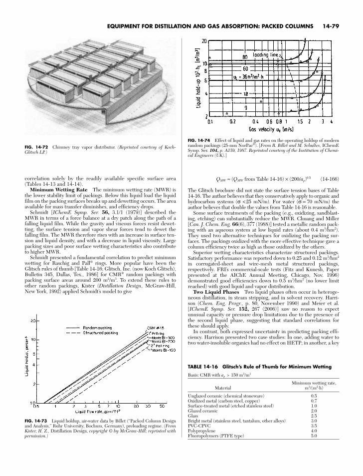
correlation solely by the readily available specific surface area(Tables 14-13 and 14-14).

Minimum Wetting Rate The minimum wetting rate (MWR) isthe lower stability limit of packings. Below this liquid load the liquidfilm on the packing surfaces breaks up and dewetting occurs. The areaavailable for mass transfer diminishes, and efficiency drops.

Schmidt [IChemE Symp. Ser. 56, 3.1/1 (1979)] described theMWR in terms of a force balance at a dry patch along the path of afalling liquid film. While the gravity and viscous forces resist dewet-ting, the surface tension and vapor shear forces tend to dewet thefalling film. The MWR therefore rises with an increase in surface ten-sion and liquid density, and with a decrease in liquid viscosity. Largepacking sizes and poor surface wetting characteristics also contributeto higher MWR.

Schmidt presented a fundamental correlation to predict minimumwetting for Raschig and Pall® rings. More popular have been theGlitsch rules of thumb [Table 14-16; Glitsch, Inc. (now Koch Glitsch),Bulletin 345, Dallas, Tex., 1986] for CMR® random packings withpacking surface areas around 200 m2/m3. To extend these rules toother random packings, Kister (Distillation Design, McGraw-Hill,New York, 1992) applied Schmidt’s model to give

QMW ≈ (QMW from Table 14-16) × (200/ap)0.5 (14-166)

The Glitsch brochure did not state the surface tension bases of Table14-16. The author believes that they conservatively apply to organic andhydrocarbon systems (σ <25 mN/m). For water (σ = 70 mN/m) theauthor believes that double the values from Table 14-16 is reasonable.

Some surface treatments of the packing (e.g., oxidizing, sandblast-ing, etching) can substantially reduce the MWR. Chuang and Miller[Can. J. Chem. Eng. 66(6), 377 (1988)] tested a metallic random pack-ing with an aqueous system at low liquid rates (about 0.4 m3/hm2).They used two alternative techniques for oxidizing the packing sur-faces. The packings oxidized with the more effective technique gave acolumn efficiency twice as high as those oxidized by the others.

Superior wetting characteristics characterize structured packings.Satisfactory performance was reported down to 0.25 and 0.12 m3/hm2

in corrugated-sheet and wire-mesh metal structured packings,respectively. FRI’s commercial-scale tests (Fitz and Kunesh, Paperpresented at the AIChE Annual Meeting, Chicago, Nov. 1996)demonstrated good efficiencies down to 0.5 m3/hm2 (no lower limitreached) with good liquid and vapor distribution.

Two Liquid Phases Two liquid phases often occur in heteroge-neous distillation, in steam stripping, and in solvent recovery. Harri-son (Chem. Eng. Progr., p. 80, November 1990) and Meier et al.[IChemE Symp. Ser. 152, 267 (2006)] saw no reason to expectunusual capacity or pressure drop limitations due to the presence ofthe second liquid phase, suggesting that standard correlations forthese should apply.

In contrast, both expressed uncertainty in predicting packing effi-ciency. Harrison presented two case studies: In one, adding water totwo water-insoluble organics had no effect on HETP; in another, a key

FIG. 14-72 Chimney tray vapor distributor. (Reprinted courtesy of Koch-Glitsch LP.)

FIG. 14-73 Liquid holdup, air-water data by Billet (“Packed Column Designand Analysis,” Ruhr University, Bochum, Germany), preloading regime. (FromKister, H. Z., Distillation Design, copyright © by McGraw-Hill; reprinted withpermission.)

FIG. 14-74 Effect of liquid and gas rates on the operating holdup of modernrandom packings (25-mm NorPac®). [From R. Billet and M. Schultes, IChemESymp. Ser. 104, p. A159, 1987. Reprinted courtesy of the Institution of Chemi-cal Engineers (UK).]

TABLE 14-16 Glitsch’s Rule of Thumb for Minimum Wetting

Basis: CMR with ap > 150 m2/m3

Minimum wetting rate,Material m3/(m2⋅h)

Unglazed ceramic (chemical stoneware) 0.5Oxidized metal (carbon steel, copper) 0.7Surface-treated metal (etched stainless steel) 1.0Glazed ceramic 2.0Glass 2.5Bright metal (stainless steel, tantalum, other alloys) 3.0PVC-CPVC 3.5Polypropylene 4.0Fluoropolymers (PTFE type) 5.0

EQUIPMENT FOR DISTILLATION AND GAS ABSORPTION: PACKED COLUMNS 14-79

component was soluble in both liquid phases, and HETP was about 50percent above normal. Harrison argued that a second liquid phaseleads to lower efficiency only when it impairs diffusion of the keyspecies. On this basis, Harrison expects efficiency loss also when an“inert” liquid or vapor represents a large fraction of the liquid or vaporphase. Meier et al. recommend obtaining efficiencies by scaling uplaboratory-scale data using a similar type of packing.

Both Harrison and Meier et al. emphasize adequately distributingeach liquid phase to the packing. Harrison noted that a well-designedladder pipe distributor can maintain high velocities and low residencetimes that provide good mixing. With trough distributors that separatethe phases and then distribute each to the packing, a light-to-heavyphase maldistribution may occur, especially when the phase ratio andseparation vary. Meier et al. noted the existence of a cloudy two-liquid

layer between the clear light and heavy liquid and recommend anadditional middle distribution point for this layer. They also noticedthat phase separation unevenness can have a large influence on thephase ratio irrigated to the packing.

High Viscosity and Surface Tension Bravo (Paper presentedat the AIChE Spring National Meeting, Houston, Tex., 1995) studieda system that had 425-cP viscosity, 350 mN/m surface tension, and ahigh foaming tendency. He found that efficiencies were liquid-phase-controlled and could be estimated from theoretical HTU models.Capacity was less than predicted by conventional methods which donot account for the high viscosity. Design equations for orifice distrib-utors extended well to the system once the orifice coefficient was cal-culated as a function of the low Reynolds number and the surfacetension head was taken into account.

14-80 EQUIPMENT FOR DISTILLATION, GAS ABSORPTION, PHASE DISPERSION, AND PHASE SEPARATION

OTHER TOPICS FOR DISTILLATION AND GAS ABSORPTION EQUIPMENT

COMPARING TRAYS AND PACKINGS

Most separations can be performed either with trays or with packings.The factors below represent economic pros and cons that favor eachand may be overridden. For instance, column complexity is a factorfavoring trays, but gas plant demethanizers that often use one or moreinterreboilers are traditionally packed.

Factors Favoring PackingsVacuum systems. Packing pressure drop is much lower than that of

trays because the packing open area approaches the tower cross-sectional area, while the tray’s open area is only 8 to 15 percent ofthe tower cross-sectional area. Also, the tray liquid head, whichincurs substantial pressure drop (typically about 50 mm of theliquid per tray), is absent in packing. Typically, tray pressure dropis of the order of 10 mbar per theoretical stage, compared to 3 to4 mbar per theoretical stage with random packings and aboutone-half of that with structured packings.

Consider a vacuum column with 10 theoretical stages, operating at70-mbar top pressure. The bottom pressure will be 170 mbar withtrays, but only 90 to 110 mbar with packings. The packed tower willhave a much better relative volatility in the lower parts, thus reduc-ing reflux and reboil requirements and bottom temperature. Thesetranslate to less product degradation, greater capacity, and smallerenergy consumption, giving packings a major advantage.

Lower-pressure-drop applications. When the gas is moved by a fanthrough the tower, or when the tower is in the suction of a com-pressor, the smaller packing pressure drop is often a controllingconsideration. This is particularly true for towers operating close toatmospheric pressure. Here excessive pressure drop in the towerincreases the size of the fan or compressor (new plant), bottlenecksthem (existing plant), and largely increases power consumption.Due to the compression ratio, pressure drop at the compressor dis-charge is far less important and seldom a controlling consideration.

Revamps. The pressure drop advantage is invaluable in vacuum col-umn revamps, can be translated to a capacity gain, an energygain, a separation improvement, or various combinations of thesebenefits. Likewise, for towers in the suction of compressors,replacing trays by packings reduces the compression ratio andhelps debottleneck the compressor.

Packings also offer an easy tradeoff between capacity and sep-aration. In the loaded sections of the tower, larger packings canovercome capacity bottlenecks at the expense of loss in separa-tion. The separation loss can often be regained by retrofittingwith smaller packings in sections of the tower that are not highlyloaded. In tray towers, changing tray spacing gives similar results,but is more difficult to do.

Foaming (and emulsion). The low gas and liquid velocities in pack-ing suppress foam formation. The large open area of the largerrandom packing promotes foam dispersal. Both attributes make

random packing excellent for handling foams. In many casesrecurrent foaming was alleviated by replacing trays by randompacking, especially when tray downcomers were poorly designed.

Switching from trays to structured packing can aggravate foam-ing. While the low gas and liquid velocities help, the solid wallsrestrict lateral movement of foams and give support to the foams.

Small-diameter columns. Columns with diameter less than 1 m(3 ft) are difficult to access from inside to install and maintain thetrays. “Cartridge” trays or an oversized diameter are often used.Either option is expensive. Cartridge trays also run into problemswith sealing to the tower wall and matching tower to tray hard-ware [Sands, Chem. Eng., p. 86 (April 2006)]. Packing is normallya cheaper and more desirable alternative.

Corrosive systems. The practical range of packing materials iswider. Ceramic and plastic packings are cheap and effective.Trays can be manufactured in nonmetals, but packing is usually acheaper and more desirable alternative.

Low liquid holdup. Packings have lower liquid holdup than dotrays. This is often advantageous for reducing polymerization,degradation, or the inventory of hazardous materials.

Batch distillation. Because of the smaller liquid holdup of packing, ahigher percentage of the liquid can be recovered as top product.

Factors Favoring TraysSolids. Trays handle solids much more easily than packing. Both gas

and liquid velocities on trays are often an order of magnitudehigher than through packing, providing a sweeping action thatkeeps tray openings clear. Solids tend to accumulate in packingvoids. There are fewer locations on trays where solids can bedeposited. Plugging in liquid distributors has been a common trou-ble spot. Cleaning trays is much easier than cleaning packings.

Not all trays are fouling-resistant. Floats on moving valve traystend to “stick” to deposits on the tray deck. Fouling-resistant trayshave large sieve holes or large fixed valves, and these should beused when plugging and fouling are the primary considerations.

There is much that can be done to alleviate plugging with ran-dom packing. Large, open packing with minimal pockets offersgood plugging resistance. Distributors that resist plugging havelarge holes (> 13-mm diameter). Such large holes are readilyapplied with high liquid flow rates, but often not practical forsmall liquid flow rates.

Maldistribution. The sensitivity of packing to liquid and gas maldis-tribution has been a common cause of failures in packed towers.Maldistribution issues are most severe in large-diameter towers,long beds, small liquid flow rates, and smaller packing. Structuredpacking is generally more prone to maldistribution than randompacking. While good distributor design, water testing, and inspec-tion can eliminate most maldistribution issues, it only takes a fewsmall details that fall through the cracks to turn success into fail-ure. Due to maldistribution, there are far more failures experienced

OTHER TOPICS FOR DISTILLATION AND GAS ABSORPTION EQUIPMENT 14-81

with packing than in trays, and it takes more trials “to get it right”than with trays. This makes trays more robust.

Complex towers. Interreboilers, intercondensers, cooling coils, andside drawoffs are more easily incorporated in trays than in packedtowers. In packed towers, every complexity requires additionaldistribution and/or liquid collection equipment.

Feed composition variation. One way of allowing for design uncer-tainties and feedstock variation is by installing alternate feedpoints. In packed towers, every alternate feed point requiresexpensive distribution equipment.

Performance prediction. Due to their sensitivity to maldistributionthere is greater uncertainty in predicting packed column perfor-mance.

Chemical reaction, absorption. Here the much higher liquidholdup on trays provides greater residence time for absorption orchemical reaction than does packing.

Turndown. Moving valve and bubble-cap trays normally give betterturndown than packings. Unless very expensive distributors areused, packed tower turndown is usually limited by distributorturndown.

Weight. Tray towers usually weigh less than packed towers, savingon the cost of foundations, supports, and column shell.

Trays vs. Random Packings The following factors generallyfavor trays compared to random packings, but not compared to struc-tured packings.

Low liquid rates. With the aid of serrated weirs, splash baffles,reverse-flow trays, and bubble-cap trays, low liquid rates can behandled better in trays. Random packings suffer from liquiddewetting and maldistribution sensitivity at low liquid rates.

Process surges. Random packings are usually more troublesomethan trays in services prone to process surges (e.g., those causedby slugs of water entering a hot oil tower, relief valve lifting, com-pressor surges, or instability of liquid seal loops). Structuredpackings are usually less troublesome than trays in such services.

Trays vs. Structured Packings The following factors generallyfavor trays compared to structured packings, but not compared to ran-dom packings.

Packing fires. The thin sheets of structured packing (typically 0.1mm) poorly dissipate heat away from hot spots. Also, cleaning,cooling, and washing can be difficult, especially when distribu-tors or packing plug up. Many incidents of packing fires duringturnarounds (while towers with structured packings were opento atmosphere) have been reported. Most of these fires wereinitiated by pyrophoric deposits, hot work (e.g., welding) abovethe packing, opening the tower while hot organics were stillpresent, and packing metallurgy that was not fire-resistant.Detailed discussion can be found in Fractionation ResearchInc. (FRI) Design Practices Committee, “Causes and Preven-tion of Packing Fires,” Chem. Eng., July 2007.

Materials of construction. Due to the thin sheets of structuredpackings, their materials of construction need to have betterresistance to oxidation or corrosion. For a service in which car-bon steel is usually satisfactory with trays, stainless steel is usuallyrequired with structured packings.

Column wall inspection. Due to their snug fit, structured packingsare easily damaged during removal. This makes it difficult toinspect the column wall (e.g., for corrosion).

Washing and purging. Thorough removal of residual liquid, washwater, air, or process gas trapped in structured packings at start-up and shutdown is more difficult than with trays. Inadequateremoval of these fluids may be hazardous.

High liquid rates. Multipass trays effectively lower the liquid load“seen” by each part of the tray. A similar trick cannot be appliedwith packings. The capacity of structured packings tends torapidly fall off at high liquid rates.

Capacity and Efficiency Comparison Kister et al. [Chem. Eng.Progr., 90(2), 23 (1994)] reported a study of the relative capacity andefficiency of conventional trays, modern random packings, and con-ventional structured packings. They found that, for each device opti-mally designed for the design requirements, a rough guide could bedeveloped on the basis of flow parameter L/G (ρG/ρL)0.5 (abcissa in

Figs. 14-31, 14-55, and 14-56) and the following tentative conclusionscould be drawn:

Flow Parameter 0.02–0.11. Trays and random packings have much the same efficiency and

capacity.2. Structured packing efficiency is about 1.5 times that of trays or

random packing.3. At a parameter of 0.02, the structured packing has a 1.3–1.4

capacity advantage over random packing and trays. This advantagedisappears as the parameter approaches 0.1.

Flow Parameter 0.1–0.31. Trays and random packings have about the same efficiency and

capacity.2. Structured packing has about the same capacity as trays and ran-

dom packings.3. The efficiency advantage of structured packing over random

packings and trays decreases from 1.5 to 1.2 as the parameterincreases from 0.1 to 0.3.

Flow Parameter 0.3–0.51. The loss of capacity of structured packing is greatest in this

range.2. The random packing appears to have the highest capacity and

efficiency with conventional trays just slightly behind. Structuredpacking has the least capacity and efficiency.

Experience indicates that use of structured packings has capacity/efficiency disadvantages in the higher-pressure (higher-flow-parame-ter) region.

Zuiderweg and Nutter [IChemE Symp. Ser. 128, A481 (1992)]explain the loss of capacity/efficiency by a large degree of backmixingand vapor recycle at high flow parameters, promoted by the solid wallsof the corrugated packing layers.

SYSTEM LIMIT: THE ULTIMATE CAPACITY OF FRACTIONATORS

Liquid drops of various sizes form in the gas-liquid contact zones oftray or packed towers. Small drops are easily entrained upward, buttheir volume is usually too small to initiate excessive liquid accumu-lation (flooding). When the gas velocity is high enough to initiate amassive carryover of the larger drops to the tray above, or upwardin a packed bed, liquid accumulation (entrainment flooding) takesplace. This flood can be alleviated by increasing the tray spacing orusing more hole areas on trays or by using larger, more open pack-ings.

Upon further increase of gas velocity, a limit is reached when thesuperficial gas velocity in the gas-liquid contact zone exceeds the set-tling velocity of large liquid drops. At gas velocities higher than this,ascending gas lifts and carries over much of the tray or packing liquid,causing the tower to flood. This flood is termed system limit or ulti-mate capacity. This flood cannot be debottlenecked by improvingpacking size or shape, tray hole area, or tray spacing. The system limitgas velocity is a function only of physical properties and liquid flowrate. Once this limit is reached, the liquid will be blown upward. Thisis analogous to spraying water against a strong wind and gettingdrenched (Yangai, Chem. Eng., p. 120, November 1990). The systemlimit represents the ultimate capacity of the vast majority of existingtrays and packings. In some applications, where very open packings(or trays) are used, such as in refinery vacuum towers, the system limitis the actual capacity limit.

The original work of Souders and Brown [Ind. Eng. Chem. 26(1),98 (1934), Eq. (14-80)] related the capacity of fractionators due toentrainment flooding to the settling velocity of drops. The concept ofsystem limit was advanced by Fractionation Research Inc. (FRI),whose measurements and model have recently been published (Fitzand Kunesh, Distillation 2001: Proceedings of Topical Conference,AIChE Spring National Meeting, Houston, Tex., 2001; Stupin, FRITopical Report 34, 1965 available through Special Collection Section,Oklahoma State University Library, Stillwater, Okla.). Figure 14-75 isa plot of FRI system limit data (most derived from tests with dual-flowtrays with 29 percent hole area and 1.2- to 2.4-m tray spacing) againstliquid superficial velocity for a variety of systems (Stupin, loc. cit.,

1965). The data show a constant-slope linear dependence of the sys-tem limit C-factor on the liquid load. There was a shortage of data atlow liquid loads. Later data (Fig. 14-76) showed that as the liquid loadwas reduced, the system limit Cs,ult stopped increasing and reached alimiting value. Based on this observation, Stupin and Kister [Trans.IChemE 81, Part A, p. 136 (January 2003)] empirically revised theearlier Stupin/FRI correlation to give

C1 = 0.445(1 − F)� 0.25

− 1.4LS (14-167)

C2 = 0.356(1 − F)� 0.25

(14-168)σ

�∆ρ

σ�∆ρ

Cs,ult = smaller of C1 and C2 (14-169)

where

F = (14-170)

In Eqs. (14-167) through (14-170), Cs,ult is the system limit C-factorbased on the tower superficial area [see Eq. (14-77) for C-factor defi-nition]; LS is the liquid superficial velocity, m/s; σ is the surface ten-sion, mN/m; ∆ρ is the difference between the liquid and gas densities,kg/m3; and ρG is the gas density, kg/m3.

Stupin and Kister (loc. cit.) relate the flattening of the curve in Fig.14-76 at low liquid loads to the formation of more, smaller, easier-to-entrain liquid drops when the liquid load is lowered beyond the limit-ing liquid load. It follows that devices that can restrict the formation ofsmaller drops may be able to approach the system limit capacity pre-dicted by Stupin’s original equation [Eq. (14-167)] even at low liquidloads.

The only devices capable of debottlenecking a tray system-limitdevice are those that introduce a new force that helps disentrain thevapor space. Devices that use centrifugal force (see “CentrifugalForce Deentrainment”) are beginning to make inroads into commer-cial distillation and have achieved capacities as high as 25 percentabove the system limit. Even the horizontal vapor push (see “Trun-cated Downcomers/Forward-Push Trays”) can help settle theentrained drops, but to a much lesser extent. It is unknown whetherthe horizontal push alone can achieve capacities exceeding the systemlimit.

WETTED-WALL COLUMNS

Wetted-wall or falling-film columns have found application in mass-transfer problems when high-heat-transfer-rate requirements areconcomitant with the absorption process. Large areas of open surface

1��

1 + 1.4(∆ρ/ρG)1/2

14-82 EQUIPMENT FOR DISTILLATION, GAS ABSORPTION, PHASE DISPERSION, AND PHASE SEPARATION

FIG. 14-75 Effect of liquid rate on ultimate capacity at higher liquid rates. (From Stupin, W. J., and H. Z. Kister, Trans. IChemE, vol. 81, Part A, p. 136,January 2003. Reprinted courtesy of IChemE.)

FIG. 14-76 Comparison of original ultimate capacity correlation to test data,C6/C7, 1.66 bar. (From Stupin, W. J., and H. Z. Kister, Trans. IChemE, vol. 81,Part A, p. 136, January 2003. Reprinted courtesy of IChemE.)

OTHER TOPICS FOR DISTILLATION AND GAS ABSORPTION EQUIPMENT 14-83

are available for heat transfer for a given rate of mass transfer in thistype of equipment because of the low mass-transfer rate inherent inwetted-wall equipment. In addition, this type of equipment lendsitself to annular-type cooling devices.

Gilliland and Sherwood [Ind. Eng. Chem., 26, 516 (1934)] foundthat, for vaporization of pure liquids in air streams for streamline flow,

= 0.023NRe0.83 NSc

0.44 (14-171)

where Dg = diffusion coefficient, ft2/hDtube = inside diameter of tube, ft

kg = mass-transfer coefficient, gas phase, lb⋅mol/(h⋅ft2) (lb⋅mol/ft3)

PBM = logarithmic mean partial pressure of inert gas, atmP = total pressure, atm

NRe = Reynolds number, gas phaseNSc = Schmidt number, gas phase

Note that the group on the left side of Eq. (14-171) is dimension-less. When turbulence promoters are used at the inlet-gas section,an improvement in gas mass-transfer coefficient for absorption ofwater vapor by sulfuric acid was observed by Greenewalt [Ind. Eng.Chem., 18, 1291 (1926)]. A falling off of the rate of mass transferbelow that indicated in Eq. (14-171) was observed by Cogan andCogan (thesis, Massachusetts Institute of Technology, 1932) when acalming zone preceded the gas inlet in ammonia absorption (Fig.14-77).

In work with the hydrogen chloride-air-water system, Dobratz,Moore, Barnard, and Meyer [Chem. Eng. Prog., 49, 611 (1953)]using a cocurrent-flow system found that Kg-G1.8 (Fig. 14-78)instead of the 0.8 power as indicated by the Gilliland equation.Heat-transfer coefficients were also determined in this study. Theradical increase in heat-transfer rate in the range of G = 30kg/(s⋅m2) [20,000 lb/(h⋅ft2)] was similar to that observed by Tepeand Mueller [Chem. Eng. Prog., 43, 267 (1947)] in condensationinside tubes.

PBM�

PkgDtube�

Dg

FIG. 14-77 Mass-transfer rates in wetted-wall columns having turbulence promoters. To convertpound-moles per hour-square foot-atmosphere to kilogram-moles per second-square meter-atmosphere,multiply by 0.00136; to convert pounds per hour-square foot to kilograms per second-square meter, mul-tiply by 0.00136; and to convert inches to millimeters, multiply by 25.4. (Data of Greenewalt and Coganand Cogan, Sherwood, and Pigford, Absorption and Extraction, 2d ed., McGraw-Hill, New York, 1952.)

FIG. 14-78 Mass-transfer coefficients versus average gas velocity—HClabsorption, wetted-wall column. To convert pound-moles per hour-square foot-atmosphere to kilogram-moles per second-square meter-atmosphere, multiplyby 0.00136; to convert pounds per hour-square foot to kilograms per second-square meter, multiply by 0.00136; to convert feet to meters, multiply by 0.305;and to convert inches to millimeters, multiply by 25.4. [Dobratz et al., Chem.Eng. Prog., 49, 611 (1953).]

14-84 EQUIPMENT FOR DISTILLATION, GAS ABSORPTION, PHASE DISPERSION, AND PHASE SEPARATION

FIG. 14-79 Liquid-film resistance in absorption of gases in wetted-wall columns. Theoretical lines are calculated for oxygenabsorption in water at 55°F. To convert feet to meters, multiply by 0.3048; °C = 5⁄9 (°F − 32). (Sherwood and Pigford, Absorptionand Extraction, 2d ed., McGraw-Hill, New York, 1952.)

Gaylord and Miranda [Chem. Eng. Prog., 53, 139M (1957)] using amultitube cocurrent-flow falling-film hydrochloric acid absorber forhydrogen chloride absorption found

Kg = � (14.172)

where Kg = overall mass-transfer coefficient, (kg⋅mol)/(s⋅m2⋅atm)Mm = mean molecular weight of gas stream at inlet to tube

Dtube = diameter of tube, mG = mass velocity of gas at inlet to tube, kg/(s⋅m2)µ = viscosity of gas, Pa⋅s

Note that the group DtubeG/µ is dimensionless. This relationship alsosatisfied the data obtained for this system, with a single-tube falling-film unit, by Coull, Bishop, and Gaylor [Chem. Eng. Prog., 45, 506(1949)].

The rate of mass transfer in the liquid phase in wetted-wall columns ishighly dependent on surface conditions. When laminar-flow conditionsprevail without the presence of wave formation, the laminar-penetrationtheory prevails. When, however, ripples form at the surface, and they

DtubeG�

µ1.66(10−5)��

Mm1.75

may occur at a Reynolds number exceeding 4, a significant rate of sur-face regeneration develops, resulting in an increase in mass-transfer rate.

If no wave formations are present, analysis of behavior of the liquid-film mass transfer as developed by Hatta and Katori [J. Soc. Chem.Ind., 37, 280B (1934)] indicates that

k� = 0.422 � (14-173)

where BF = (3uΓ/ρ2g)1/3

Dl = liquid-phase diffusion coefficient, m2/sρ = liquid density, kg/m3

Z = length of surface, mkl = liquid-film-transfer coefficient,

(kg⋅mol)/[(s⋅m2)(kg⋅mol)/m3]Γ = liquid-flow rate, kg/(s⋅m) based on wetted perimeterµ = viscosity of liquid, Pa⋅sg = gravity acceleration, 9.81 m/s2

D�Γ�ρBF

2

OTHER TOPICS FOR DISTILLATION AND GAS ABSORPTION EQUIPMENT 14-85

When Z is large or Γ/ρBF is so small that liquid penetration is complete,

k� = 11.800 D�/BF (14-174)

and

H� = 0.95 ΓBF/D� (14-175)

A comparison of experimental data for carbon dioxide absorptionobtained by Hatta and Katori (op. cit.), Grimley [Trans. Inst. Chem.Eng., 23, 228 (1945)], and Vyazov [Zh. Tekh. Fiz. (U.S.S.R.), 10,1519 (1940)] and for absorption of oxygen and hydrogen by Hodgson(S.M. thesis, Massachusetts Institute of Technology, 1949), Henley(B.S. thesis, University of Delaware, 1949), Miller (B.S. thesis, Uni-versity of Delaware, 1949), and Richards (B.S. thesis, University ofDelaware, 1950) was made by Sherwood and Pigford (Absorptionand Extraction, McGraw-Hill, New York, 1952) and is indicated inFig. 14-79.

In general, the observed mass-transfer rates are greater than thosepredicted by theory and may be related to the development of surfacerippling, a phenomenon which increases in intensity with increasingliquid path.

Vivian and Peaceman [Am. Inst. Chem. Eng. J., 2, 437 (1956)]investigated the characteristics of the CO2-H2O and Cl2-HCl, H2Osystem in a wetted-wall column and found that gas rate had no effecton the liquid-phase coefficient at Reynolds numbers below 2200.Beyond this rate, the effect of the resulting rippling was to increasesignificantly the liquid-phase transfer rate. The authors proposed abehavior relationship based on a dimensional analysis but suggestedcaution in its application concomitant with the use of this type of rela-tionship. Cognizance was taken by the authors of the effects of col-umn length, one to induce rippling and increase of rate of transfer,one to increase time of exposure which via the penetration theorydecreases the average rate of mass transfer in the liquid phase. Theequation is

= 0.433 � 1/2

� 1/6

� 0.4

(14-176)

where D� = diffusion coefficient of solute in liquid, ft2/hg = gravity-acceleration constant, 4.17 � 108 ft/h2

h = length of wetted wall, ftk� = mass-transfer coefficient, liquid phase, ft/h

4Γ�µ�

ρ�2 gh3

�µ�

2

µ��ρ�D�

k�h�D�

Γ = mass rate of flow of liquid, lb/(h)(ft of periphery)µ� = viscosity of liquid, lb/(ft)(h)ρ� = density of liquid, lb/ft3

The equation is dimensionless.The effect of chemical reaction in reducing the effect of variation

of the liquid rate on the rate of absorption in the laminar-flowregime was illustrated by the evaluation of the rate of absorption ofchlorine in ferrous chloride solutions in a wetted-wall column byGilliland, Baddour, and White [Am. Inst. Chem. Eng. J., 4, 323(1958)].

Flooding in Wetted-Wall Columns When gas and liquid are incounterflow in wetted-wall columns, flooding can occur at high gasrates. Methods for calculating this flood are given in “Upper LimitFlooding in Vertical Tubes.” In the author’s experience, Eq. (14-204)has had an excellent track record for calculating flooding in thesecolumns.

COLUMN COSTS

Estimation of column costs for preliminary process evaluationsrequires consideration not only of the basic type of internals but also oftheir effect on overall system cost. For a distillation system, for exam-ple, the overall system can include the vessel (column), attendantstructures, supports, and foundations; auxiliaries such as reboiler, con-denser, feed heater, and control instruments; and connecting piping.The choice of internals influences all these costs, but other factorsinfluence them as well. A complete optimization of the system requiresa full-process simulation model that can cover all pertinent variablesinfluencing economics.

Cost of Internals Installed costs of trays may be estimated fromFig. 14-80, with corrections for tray material taken from Table 14-17.For two-pass trays the cost is 15 to 20 percent higher. Approximatecosts of random packing materials may be obtained from Table 14-18,but it should be recognized that, because of competition, there can besignificant variations in these costs from vendor to vendor. Also, pack-ings sold in very large quantities carry discounts. In 1995, costs ofstructured packings, made from sheet metal, averaged $90 to $110 percubic foot, but the need for special distributors and redistributors candouble the cost of structured-packings on a volumetric basis. Note

TABLE 14-17 Relative Fabricated Cost for Metals Used in Tray-Tower Construction*

Relative costper ft2 of tray

area (based onMaterials of construction carbon steel = 1)

Sheet-metal traysSteel 14–6% chrome—a moly alloy steel 2.111–13% chrome type 410 alloy steel 2.6Red brass 3Stainless steel type 304 4.2Stainless steel type 347 5.1Monel 7.0Stainless steel type 316 5.5Inconel 8.2

Cast-iron trays 2.8

*Peters and Timmerhaus, Plant Design and Economics for Chemical Engi-neers, 4th ed., McGraw-Hill, New York, 1991. To convert cost per square foot tocost per square meter, multiply by 10.76.

TABLE 14-18 Costs of Random Packings, Uninstalled, January 1990

Prices in dollars per ft3, 100 ft3 orders, f.o.b. manufacturing plant

Size, in, $/ft3

1 1a 2 3

Raschig ringsChemical porcelain 12.8 10.3 9.4 7.8Carbon steel 36.5 23.9 20.5 16.8Stainless steel 155 117 87.8 —Carbon 52 46.2 33.9 31.0

Intalox saddlesChemical stoneware 17.6 13.0 11.8 10.7Chemical porcelain 18.8 14.1 12.9 11.8Polypropylene 21.2 — 13.1 7.0

Berl saddlesChemical stoneware 27.0 21.0 — —Chemical porcelain 33.5 21.5 15.6 —

Pall ringsCarbon steel 29.3 19.9 18.2 —Stainless steel 131 99.0 86.2 —Polypropylene 21.2 14.4 13.1

Peters and Timmerhaus, Plant Design and Economics for Chemical Engi-neers, 4th ed., McGraw-Hill, New York, 1991. To convert cubic feet to cubicmeters, multiply by 0.0283; to convert inches to millimeters, multiply by 25.4;and to convert dollars per cubic foot to dollars per cubic meter, multiply by 35.3.

14-86 EQUIPMENT FOR DISTILLATION, GAS ABSORPTION, PHASE DISPERSION, AND PHASE SEPARATION

that for Fig. 14-80 and Table 14-17, the effective cost date is January1990, with the Marshall and Swift cost index being taken as 904.

As indicated above, packed column internals include liquid distribu-tors, packing support plates, redistributors (as needed), and holddownplates (to prevent movement of packing under flow conditions). Costs ofthese internals for columns with random packing are given in Fig. 14-81,based on early 1976 prices, and a Marshall and Swift cost index of 460.

Cost of Column The cost of the vessel, including heads,skirt, nozzles, and ladderways, is usually estimated on the basisof weight. Figure 14-82 provides early 1990 cost data for theshell and heads, and Fig. 14-83 provides 1990 cost data forconnections. For very approximate estimates of completecolumns, including internals, Fig. 14-84 may be used. As forFigs. 14-82 and 14-83, the cost index is 904.

104

103

102

1 2 3 4 5 6 7 8 1511 12 13 149 10

Tower diameter, ft

Inst

alle

d co

st, d

olla

rs/tr

ay

Bubble-cap trays(stainless steel)

Quantity factors apply to all types of trays

1234567

3.002.802.652.502.302.152.00

89

1011121314

1.801.651.501.451.401.351.30

1516171819203040+

2939

1.251.201.151.101.051.000.980.97

Stamped turbogridtrays (stainless steel)

Valve trays(stainless steel)

Sieve trays(stainless steel)

Bubble-cap trays(carbon steel)

or

Valve trays(carbon steel)

Sieve trays(carbon steel)

FIG. 14-80 Cost of trays. Price includes tray deck, valves, bubble caps, risers, downcomers, and structural-steelparts. The stainless steel designated is type 410 (Peters and Timmerhaus, Plant Design and Economics for Chemi-cal Engineers, 4th ed., McGraw-Hill, New York, 1991).

PHASE DISPERSION

GENERAL REFERENCES: For an overall discussion of gas-liquid breakupprocesses, see Brodkey, The Phenomena of Fluid Motions, Addison-Wesley,Reading, Massachusetts, 1967. For a discussion of atomization devices and howthey work, see Masters, Spray Drying Handbook, 5th ed., Wiley, New York,1991; and Lefebvre, Atomization and Sprays, Hemisphere, New York, 1989. Abeautifully illustrated older source is Dombrowski and Munday, Biochemicaland Biological Engineering Science, vol. 2, Academic Press, London, 1968, pp.209–320. Steinmeyer [Chem. Engr. Prog., 91(7), 72–80 (1995)] built on Hinze’swork with turbulence and showed that several atomization processes follow thecommon theme of breakup of large droplets due to turbulence in the gas phase.Turbulence in turn correlates with power dissipation per unit mass. In the textbelow, correlations referring to power/mass are taken from this source. For asurvey on fog formation, see Amelin, Theory of Fog Formation, Israel Programfor Scientific Translations, Jerusalem, 1967.

BASICS OF INTERFACIAL CONTACTORS

Steady-State Systems: Bubbles and Droplets Bubbles aremade by injecting vapor below the liquid surface. In contrast,droplets are commonly made by atomizing nozzles that inject liquidinto a vapor. Bubble and droplet systems are fundamentally differ-ent, mainly because of the enormous difference in density of theinjected phase. There are situations where each is preferred. Bubblesystems tend to have much higher interfacial area as shown byExample 16 contrasted with Examples 14 and 15. Because of theirhigher area, bubble systems will usually give a closer approach toequilibrium.

PHASE DISPERSION 14-87

(b)(a)

FIG. 14-81 Cost of internal devices for columns containing random packings. (a) Holddown plates and support plates. (b) Redistributors. [Pikulik and Diaz,Chem. Eng., 84(21), 106 (Oct. 10, 1977).]

FIG. 14-83 Approximate installed cost of steel-tower connections. Valuesapply to 2070-kPa connections. Multiply costs by 0.9 for 1035-kPa (150-lb) con-nections and by 1.2 for 4140-kPa (600-lb) connections. To convert inches to mil-limeters, multiply by 25.4; to convert dollars per inch to dollars per centimeter,multiply by 0.394. (Peters and Timmerhaus, Plant Design and Economics forChemical Engineers, 4th ed., New York, McGraw-Hill, 1991.)

FIG. 14-82 Fabricated costs and installation time of towers. Costs are for shellwith two heads and skirt, but without trays, packing, or connections. (Peters andTimmerhaus, Plant Design and Economics for Chemical Engineers, 4th ed.,McGraw-Hill, New York, 1991.)

However, droplet systems can enable much higher energy input(via gas phase pressure drop in cocurrent systems) and, as a result,dominate applications where a quick quench is needed. See Examples21 and 22. Conversely, droplet systems can also be designed for verylow pressure drop which is advantageous in applications such as vac-uum condensers.

Unstable Systems: Froths and Hollow Cone AtomizingNozzles We usually think of interfacial contact as a steady-state system of raining droplets or rising bubbles, but some of the most effi-cient interfacial contactors take advantage of unstable interfacialgeometry. The most common is the distillation tray which operateswith a wild mix of bubbles, jets, films, and droplets. The mix is oftendescribed as froth. Gas pressure drop provides the energy to createthe froth.

A variant on the froth contact is the reverse jet contactor (Example22), which can be considered as an upside-down distillation tray, oper-ated above the flooding velocity in cocurrent flow of gas and liquid. Itis limited to one stage.

An entirely different unstable contactor involves the thin expandingliquid film produced by a hollow cone spray nozzle. Because of fresh sur-face and the thinness of the film, this can give very high transfer for liq-uid-limited systems. Two applications are direct contact condensationand removal of volatile components from a high-boiling residual liquid.

Surface Tension Makes Liquid Sheets and Liquid ColumnsUnstable Surface tension is the energy required to make an incre-ment of interfacial surface. A sheet or column of liquid has more sur-face than a sphere, hence surface tension converts sheets and columnsto droplets. See Fig. 14-86.

There are many different atomizers, but the underlying principle ofall is the same—to first generate a flat sheet or a liquid column. Liquidsheets and columns are unstable, a small surface disturbance on eitherwill propagate, and the liquid will reshape itself into droplets. The keyproperty in controlling this process is surface tension. Surface tensiongets a high exponent in all the atomization correlations.

Little Droplets and Bubbles vs. Big Droplets and Bubbles—Coalescence vs. Breakup When big drops are subjected to shearforces, as in falling rain, the droplets are distorted; and if the distor-

tions are great enough, the big droplets break into little ones. This iswhy raindrops never exceed a certain size. A variant on this is breakupin highly turbulent systems such as in high-velocity quench systems orpneumatic nozzles. Here the droplets are distorted by the energy ofthe turbulent eddies.

But little droplets and bubbles have more surface per unit of liquidthan big ones. Hence little droplets tend to coalesce into big ones, andwill grow in size if given enough quiet time.

While the primary difficulty is estimating the interfacial area due tothe unstable interface, a secondary problem is that freshly made,unstable surface gives higher transfer than older, more stable surface.

Empirical Design Tempered by Operating Data The net ofthese is that interfacial area is difficult to predict and interfacial con-tactors are difficult to design.

Prediction methods are given below but should always be temperedby operating experience.

INTERFACIAL AREA—IMPACT OF DROPLET OR BUBBLE SIZE

Transfer is aided by increased interfacial area. Interfacial area per unitvolume aD of a single droplet or bubble is inversely proportional to thediameter of the droplet or bubble D.

aD = 6/D (14-177)

To estimate the total interfacial area in a given volume, the ad value ismultiplied by the fractional holdup of dispersed phase in the totalvolume.

a = aD(ΦD) (14-178)

where a = interfacial area/volume and ΦD = fraction of volume in dis-persed phase = holdup. Fractional holdup in a continuous processdepends on the velocities of the two phases, as if they were flowing bythemselves.

ΦD = (dispersed phase volume)/(volume of dispersed and continuous phases)

Example 14: Interfacial Area for Droplets/Gas in CocurrentFlow For equal mass flow of gas and liquid and with gas density 0.001 of liq-uid density, the gas velocity in cocurrent flow will be 1000 times the liquid veloc-ity. This sets ΦD.

ΦD = 1/(1 + 1000) = 0.00099

If the droplets are 500 µm in diameter, Eqs. (14-177) and (14-178) give

a = (6/0.0005)(0.00099) = 12 m2/m3

If the droplets are 100 µm in diameter, Eqs. (14-177) and (14-178) give

a = (6/0.0001)(0.00099) = 60 m2/m3

Example 15: Interfacial Area for Droplets Falling in a VesselDroplet systems rarely exceed a ΦD value of 0.01. At this low level, ΦD in a low-velocity countercurrent contactor can be approximated by Eq. (14-179).

ΦD = UL/(Ut − UG) (14-179)

where UL = liquid superficial velocityUt = terminal velocity of droplet

UG = gas superficial velocity

With a gas superficial velocity of 1.5 m/s, for equal mass flow of gas and liquid,with gas density 0.001 of liquid density, and with 500-µm-diameter dropletsfalling at a terminal settling of 2.5 m/s, Eq. (14-179) gives a fractional holdup ofliquid of

ΦD = (0.001)1.5/(2.5 − 1.5) = 0.0015

Equations (14-177) and (14-178) then give

a = (6/0.0005)(0.0015) = 18 m2/m3

Example 16: Interfacial Area for Bubbles Rising in a VesselFor bubble systems (gases dispersed in liquids) fractional holdup can approach0.5 as shown by Fig. 14-104. However, before reaching this holdup, the bubblesystems shift to an unstable mix of bubbles and vapor jets. Hence an exact

14-88 EQUIPMENT FOR DISTILLATION, GAS ABSORPTION, PHASE DISPERSION, AND PHASE SEPARATION

FIG. 14-84 Cost of towers including installation and auxiliaries. To convertinches to millimeters, multiply by 25.4; to convert feet to meters, multiply by0.305; and to convert dollars per foot to dollars per meter, multiply by 3.28.(Peters and Timmerhaus, Plant Design and Economics for Chemical Engineers,4th ed., McGraw-Hill, New York, 1991.)

PHASE DISPERSION 14-89

comparison to Example 14 isn’t possible because at the 1.5 m/s velocity ofExample 14, the system becomes a froth. But at about one-fifth the velocity ofExample 14, an estimate of interfacial area is possible.

If the bubble size is 10,000 µm and fractional holdup is 0.4, Eqs. (14-177) and(14-178) give an interfacial area of

a = (6/0.01)(0.4) = 240 m2/m3

Measured interfacial area in distillation trays is consistent with this high value.Note the much higher interfacial area than in the droplet systems of

Examples 14 and 15. The higher interfacial area when the gas is dispersedexplains why bubbling and froth systems often give better performancethan droplet systems. The big difference in interfacial area stems from themuch larger volume per unit of mass of gas, i.e., lower density of the gasthan the liquid.

RATE MEASURES, TRANSFER UNITS, APPROACH TO EQUILIBRIUM, AND BYPASSING

What Controls Mass/Heat Transfer: Liquid or Gas Transferor Bypassing Either gas side or liquid side of the interface can becontrolling.

Liquid-Controlled In fractionation systems with high viscosityor component relative volatility that greatly exceeds 1, the liquid sidewill be controlling. This is clearly illustrated by Fig. 14-47 whichshows a sharp decline in efficiency with either a rise in liquid viscosityor a rise in component relative volatility.

Note that high component relative volatility means the samething as sparingly soluble. Oxygen dissolving in a fermentationreactor is an example of a system being liquid-controlled due to asparingly soluble gas. Another application that is liquid-controlledis the removal of high relative volatility components out of residualoil.

Still another case where liquid controls is in condensing a purevapor, as in Example 23, or absorbing a pure gas, as in Example 24.

Gas-Controlled The gas side dominates in gas cooling applica-tions. An example is the quenching of a furnace effluent with a vapor-izing liquid. In this application the liquid is nearly uniform intemperature. Restated, the reduction in driving force across the liquidside of the interface is unimportant.

Other applications that are gas-side-controlled include removal of acomponent such as NH3 from a gas by using an acidic liquid, orremoving a component such as SO2 from a gas with a basic liquid. SeeExamples 19 through 22.

Bypassing-Controlled Trayed or packed columns operate withcountercurrent flow and can achieve many equilibrium stages inseries by good distribution of gas and liquid, and careful control ofdetails. Other devices such as sprays are vulnerable to bypassing andare limited to one equilibrium stage.

Rate Measures for Interfacial Processes Terminology usedfor reporting rate data can be confusing. Normally rate data arereported on a volumetric basis with transfer rate and effective areacombined. For example, kLa denotes mass-transfer data per unit vol-ume. The L subscript means it is referenced to the molar concentra-tion difference between the interface and the bulk liquid. This iscommonly used on data involving a sparingly soluble (high relativevolatility) component. Note that the lowercase k means the data dealonly with the resistance in the liquid phase.

Less commonly, data are given as kGa. The G subscript means it isreferenced to the molar concentration difference between the inter-face and the gas. This might be used for data on absorbing a gas suchas NH3 by a highly acidic liquid. Note that kGa only deals with theresistance in the gas phase.

When one is dealing with direct contact heat transfer, the corre-sponding terms are hLa and hGa. Here the driving force is the tem-perature difference. The L subscript means that we are dealing with aliquid-limited process such as condensing a pure liquid. How to con-vert kLa data to an hLa value is illustrated by Example 23.

There are ways to combine the liquid and gas resistance to get anoverall transfer rate such as KGa (as denoted by the uppercase K).However, data are rarely reported in this form.

Approach to Equilibrium Although rate measures such as kGaand hGa are often cited in the literature, they are often not as useful todesigners as the simpler concept of approach to equilibrium. Approachto equilibrium compares the transfer between liquid and gas phases tothe best possible that could be achieved in a single backmixed equi-librium stage.

Approach to equilibrium is easy to understand and easy to apply.Examples 17 through 23 illustrate its use.

Example 17: Approach to Equilibrium—Perfectly Mixed, Com-plete Exchange This would be approximated by a very long pipeline contac-tor where an acidic aqueous stream is injected to cool the gas and remove NH3.

If the adiabatic saturation temperature of the gas is 70°C, at the exit of thecontactor, the gas would be cooled to 70°C.

Similarly, at the exit of the contactor, the NH3 in the gas would be zero,regardless of the initial concentration.

Example 18: Approach to Equilibrium—Complete Exchangebut with 10 Percent Gas Bypassing A spray column is used, and anacidic liquid rains down on the gas of Example 17. If the initial NH3 is 1000 ppmand 10 percent of the gas bypasses, the NH3 in the exit gas would be

0.1(1000) = 100 ppmSimilarly, if the gas enters at 120°C, at the exit we would find 10 percent of thedifferential above the adiabatic saturation temperature. For an adiabatic satura-tion temperature of 70°C, the exit gas temperature would be

70 + 0.1(120 − 70) = 75°C

Approach to Equilibrium—Finite Contactor with No Bypass-ing When there is no bypassing, the measure that sets the approachis the ratio of change to driving force. This ratio is called the numberof transfer units NG. It is dimensionless. For heat-transfer applica-tions, it can be envisioned as a conventional heat exchanger where avaporizing liquid cools a gas:

No. of gas-phase transfer units = = NG (14-180)

Where TG = gas temperature and TL = liquid temperature. Thenumber of transfer units NG can also be calculated as the capabilityfor change divided by the thermal capacitance of the flowingstreams.

NG =

= (14-181)

where a = interfacial area per unit volumehG = heat-transfer coefficient from interface to gasρG = gas densitycG = gas specific heat

Note that in the above, performance and properties all refer to thegas, which is appropriate when dealing with a gas-limited transferprocess.

This leads to a way to estimate the approach to equilibrium.

E = 1 − e−NG (14-182)

where E = “approach to equilibrium” fractional removal of NH3 orfractional approach to adiabatic liquid temperature

NG = number of transfer units calculated relative to gas flow

Example 19: Finite Exchange, No Bypassing, Short ContactorA short cocurrent horizontal pipeline contactor gives 86 percent removal ofNH3. There is no bypassing because of the highly turbulent gas flow and injec-tion of liquid into the center of the pipe. What would we expect the exit gas tem-perature to be?

(gas contact time)(hGa)���

ρGcG

(system volume)(hGa)���(volumetric flow rate)ρGcG

TG,out − TG,in��

(TG − TL)av

Equation (14-182) says that the backcalculated NG is 2:

NG = −ln(1 − 0.86) = 2

For diffusing gases of similar molecular weight, the properties that controlheat transfer follow the same rules as those that control mass transfer. As aresult, the NH3 scrubbing and gas cooling processes achieve similar approachesto equilibrium.

For an entry temperature of 120°C and an adiabatic saturation temperatureof 70°C, the expected outlet temperature would be

70 + (1 − 0.86)(120 − 70) = 77°C

This looks like a powerful concept, but its value is limited due to uncer-tainty in estimating hGa. Both hG and a are difficult to estimate due todependence on power dissipation as discussed below. The primaryvalue of the NG concept is in estimating an expected change from base-line data as in the comparison of Example 19 with Example 20.

Example 20: A Contactor That Is Twice as Long, No Bypass-ing If we double the length of the pipeline contactor, double the effectivecontact area, and double the number of transfer units to 4, what do we expectfor performance?

For NG = 4,

E = 1 − e−4 = 0.982

The NH3 in the exit gas would be expected to drop to

(1 − 0.982)(1000) = 18 ppm

and the expected outlet temperature would be

70 + (1 − 0.982)(120 − 70) = 70.9°C

If we double the length again, we increase the number of transfer units to 8 andachieve an approach of

E = 1 − e−8 = 0.9997

The outlet temperature would be

70 + (1 − 0.9997)(120 − 70) = 70.015°C

Similarly the NH3 in the exit gas would be

(1 − 0.9997)(1000) = 0.3 ppm

Note that this approximates the exit condition of Example 17.

Transfer Coefficient—Impact of Droplet Size The transfercoefficients increase as the size of droplets decreases. This is sobecause the transfer process is easier if it only has to move mass orheat a shorter distance (i.e., as the bubble or droplet gets smaller).

In the limiting case of quiescent small bubbles or droplets, thetransfer coefficients vary inversely with average bubble or dropletdiameter. For example, in heat transfer from a droplet interface to agas, the minimum value is

hG,min = heat transfer coefficient from interface to gas = 2kG/D(14-183)

where kG = gas thermal conductivity and D = droplet diameter.

IMPORTANCE OF TURBULENCE

The designer usually has control over the size of a droplet. As dis-cussed below, several of the correlations show that droplet diametervaries with turbulent energy dissipation. For example, Eqs. (14-190)and (14-201) suggest that in droplet systems

D ∝ {1/(gas velocity)]1.2

and hence from Eq. (14-178)

a ∝ 1/D ∝ (gas velocity)1.2 (14-184)

However, just looking at the impact of velocity on droplet size under-estimates the velocity impact because turbulence gives higher transfer

than Eq. (14-183) predicts. Transfer coefficients increase as the mix-ing adjacent to the surface increases. This mixing depends on theenergy dissipated into the phases. To a first approximation this trans-fer from droplets increases with local power dissipation raised to the0.2 power.

hG,turbulent ∝ (power dissipated)0.2

and since power dissipation per unit volume increases with (velocity)3,

hG,turbulent ∝ (velocity)0.6 (14-185)

The combined effect on interfacial area and on the transfer coefficientis that the effective transfer increases greatly with gas velocity. FromEqs. (14-178) and (14-185)

hGaturbulent ∝ (velocity)1.8 (14-186)

For quenching operations, this means that even though residencetime is cut as gas velocity goes up, the effective approach to equilib-rium increases. Since the volume for a given length of pipe falls with(velocity)−1, the expected number of transfer units NG in a given lengthof pipe increases with (velocity)0.8

.

NG,turbulent ∝ (hGaturbulent)(volume) ∝ (velocity)0.8 (14-187)

See Example 21.

EXAMPLES OF CONTACTORS

High-Velocity Pipeline Contactors High-velocity cocurrentflow can give more power input than any other approach. This iscritical when extremely high rates of reaction quenching areneeded.

Example 21: Doubling the Velocity in a Horizontal PipelineContactor—Impact on Effective Heat Transfer Velocity in pipelinequench systems often exceeds 62 m/s (200 ft/s). Note that this is far above theflooding velocity in distillation packing, distillation trays, or gas-sparged reac-tors. There are few data available to validate performance even though liquidinjection into high-velocity gas streams has been historically used in quenchingreactor effluent systems. However, the designer knows the directional impact ofparameters as given by Eq. (14-187).

For example, if a 10-ft length of pipe gives a 90 percent approach to equilib-rium in a quench operation, Eq. (14-182) says that the backcalculated NG is2.303:

NG −ln(1 − 0.9) =2.303

Equation (14-187) says if we double velocity but retain the same length, wewould expect an increase of NG to 4.0.

NG = 2.303(2)0.8 = 4and

E = 1 − e−4 = 0.982

Restated, the approach to equilibrium rises from 90 percent to greater than 98percent even though the contact time is cut in half.

Vertical Reverse Jet Contactor A surprisingly effectivemodification of the liquid injection quench concept is to inject theliquid countercurrent upward into a gas flowing downward, withthe gas velocity at some multiple of the flooding velocity definedby Eq. (14-203). The reverse jet contactor can be envisioned as anupside-down distillation tray. For large gas volumes, multipleinjection nozzles are used. One advantage of this configuration isthat it minimizes the chance of liquid or gas bypassing. Anotheradvantage is that it operates in the froth region which generatesgreater area per unit volume than the higher-velocity cocurrentpipeline quench.

The concept was first outlined in U.S. Patent 3,803,805 (1974) andwas amplified in U.S. Patent 6,339,169 (2002). The 1974 patent pre-sents data which clarify that the key power input is from the gas stream.

A more recent article discusses use of the reverse jet in refinery offgasscrubbing for removal of both SO2 and small particles [Hydrocarbon

14-90 EQUIPMENT FOR DISTILLATION, GAS ABSORPTION, PHASE DISPERSION, AND PHASE SEPARATION

PHASE DISPERSION 14-91

Processing, 84,(9), 99–106 (2005)]. This article cites downward gasvelocities in the range of 10 to 37 m/s and notes gas pressure drop in therange of 6 to 20 in of water. Removals of SO2 and fine particles were bothclose to 99 percent. The froth produced by the contactor reverses direc-tion, flows down, and is largely disengaged in a vessel mounted below.

Example 22: The Reverse Jet Contactor, U.S. Patent 6,339,169This patent deals with rapid cooling and removal of NH3 from gas exiting anacrylonitrile reactor. Liquid is injected upward. The claims suggest downward-flowing gas velocity is between 20 and 25 m/s.

Gas cooling is reported to be largely complete in 0.1 s. NH3 removal at theexit of the contactor is reported to be greater than 99 percent. The gas is cooledby water vaporizing from the injected liquid, with total water circulated being inthe range of 100 times that evaporated.

Since the gas cooling and NH3 scrubbing move in parallel, they would beexpected to achieve nearly the same approach to equilibrium as long as the pHof all the liquid stays below a key threshold. The great excess of liquid enables this.

The key is high froth interfacial area per unit volume.

Simple Spray Towers The other extreme to the pipeline andreverse jet contactors is an open vessel where spray is injected down intoupflowing gas to form a rain of liquid. The advantage of simple spray tow-ers is that they give low gas pressure drop and also tend to be nonfouling.

Even though gas velocity is well below flooding velocity, the finerdroplets of the spray will be entrained. Note the wide spectrum ofparticle sizes shown by Fig. 14-88.

However, as shown by Examples 23 and 24, they can be extremelyeffective in liquid-limited systems.

Bypassing Limits Spray Tower Performance in Gas CoolingAs shown by Example 18, only modest performance is achieved in gas-limited systems. The modest efficiency is due to gas bypassing. Tallspray towers are not effective countercurrent devices. Even withnominally falling droplets, there is a great deal of backmixing becausethere is no stabilizing pressure drop as there would be in a columnfilled with packing or trays. A packet of droplets weighs more than agas-filled space. The result is that the volume that is filled with themost droplets moves down relative to all other volumes. Similarly thegas volume that has fewest droplets moves up more quickly thanother volumes. This generates bypassing of liquid and gas. The flowsare driven by the rain of droplets themselves. Anything less than per-fect distribution of liquid and gas will induce a dodging actionbetween the flowing streams. Most designers limit expectations forspray contactors to some fraction of a single equilibrium stageregardless of height.

One approach that has been employed to get better distribution inspray systems is to mount a single large-capacity nozzle in the centerof the vessel with radial discharge of large droplets. The droplets aredischarged with enough velocity to penetrate to the vessel walls.

Spray Towers in Liquid-Limited Systems—Hollow ConeAtomizing Nozzles If we follow an element of liquid leaving a hol-low cone hydraulic spray nozzle, the sequence is a rapidly thinningcone followed by wave development, followed by shedding of liga-ments, followed by breakage of the ligaments into droplets. See Fig.14-86. The sequence gives high transfer for liquid-limited systems.This results from the thin sheet of the hollow cone as well as the cre-ation of fresh surface in the breakup process.

Devolatilizers Devolatilization systems are liquid-limited due tothe combination of high liquid viscosity and removal of a componentwith high relative volatility. Simpson and Lynn [AIChE J., 23 (5),666–673 (1977)] reported oxygen stripping from water at 98 percentcomplete, in less than 1 ft of contact. The concept has been employedfor residual devolatilization in refineries.

Spray Towers as Direct Contact Condensers Similarly spraycontactors can be highly effective for direct contact condensers, whichare also liquid-limited. The high transfer rate in the initial formationof sprays is the key. Kunesh [Ind. Engr. Chem. Res., 32, 2387–2389(1993)] reported a 97 percent approach to equilibrium in a hydrocar-bon system in the 6-in space below the discharge of a row of hollowcone spray nozzles.

Other results on heat transfer in a large spray condenser are givenby Waintraub et al. (“Removing Packings from Heat Transfer Sectionsof Vacuum Towers,” AIChE 2005 Spring National Meeting, Proceed-

ings of Topical Conference, April 10, 2005, Atlanta, p. 79). The paperhighlights the importance of good gas and liquid distribution.

Converting Liquid Mass-Transfer Data to Direct ContactHeat Transfer Liquid-limited performance measures are muchmore commonly given for mass-transfer than for heat transfer. Oftenmass-transfer data are reported as kLa with units of h−1. This can beconverted to hLa with units of Btu/(h⋅°F⋅ft3) by Eq. (14-188).

hLa = 187(kLa) (cL) (ρL) (µL/T)0.5 (14-188)

where µL = liquid, cPT = temperature, °RρL = liquid density, lb/ft3

cL = liquid specific heat, Btu/(lb⋅°F)

Calculation of transfer units for heat transfer is relatively simple. Fora liquid

NL = (14-189)

where ρL = liquid density and cL = liquid specific heat. [See parallelgas expression, Eq. (14-181).]

Unlike gases, the liquid properties that control mass and heat trans-fer differ greatly. The key term is diffusivity which for liquids dropswith viscosity.

The resulting values for hLa and NL can be surprisingly large whena pure vapor such as steam is condensed. See Example 23.

Example 23: Estimating Direct Contact Condensing Perfor-mance Based on kLa Mass-Transfer Data If an aqueous system at560°R gives a kLa of 60 h−1, what does Eq. (14-188) predict for hLa in a directcontact steam condenser?

For an aqueous system

µL = 1 cP

ρL = 62 lb/ft3

cL = 1 Btu/(lb⋅°F)

and Eq. (14-189) predicts

hLa = 187(60)(1)(62)(1/560)0.5 = 29,400 Btu/(h⋅°F⋅ft3)

When a pure gas such as HCl is absorbed by low viscosity liquidsuch as water, simple spray systems can also be highly effective. SeeExample 24.

Example 24: HCl Vent Absorber (Kister, Distillation Troubleshoot-ing, Wiley, 2006, p. 95.) A 6-in-diameter, 8-ft-tall packed bed was giving majorproblems due to failure of the packing support. Water was the scrubbing fluid.

The liquid distributors were replaced with carefully positioned spray nozzles,and the packing was removed. HCl in the vent was removed to a level one-fortieth of the original design.

LIQUID-IN-GAS DISPERSIONS

Liquid Breakup into Droplets There are four basic mecha-nisms for breakup of liquid into droplets:• Droplets in a field of high turbulence (i.e., high power dissipation

per unit mass)• Simple jets at low velocity• Expanding sheets of liquid at relatively low velocity• Droplets in a steady field of high relative velocityThese mechanisms coexist, and the one that gives the smallest dropsize will control. The four mechanisms follow distinctly differentvelocity dependencies:

1. Breakup in a highly turbulent field (1/velocity)1.2. This appears tobe the dominant breakup process in distillation trays in the sprayregime, pneumatic atomizers, and high-velocity pipeline contactors.

2. Breakup of a low-velocity liquid jet (1/velocity)0. This governs inspecial applications like prilling towers and is often an intermediatestep in liquid breakup processes.

3. Breakup of a sheet of liquid (1/velocity)0.67. This governs dropsize in most hydraulic spray nozzles.

(liquid contact time)(hLa)���

ρLcL

4. Single-droplet breakup at very high velocicty (1/velocity)2. Thisgoverns drop size in free fall as well as breakup when droplets impingeon solid surfaces.

Droplet Breakup—High Turbulence This is the dominantbreakup mechanism for many process applications. Breakup resultsfrom local variations in turbulent pressure that distort the dropletshape. Hinze [Am. Inst. Chem. Eng. J., 1, 289–295 (1953)] appliedturbulence theory to obtain the form of Eq. (14-190) and took liquid-liquid data to define the coefficient:

Dmax = 0.725(σ/ρG)0.6/E0.4 (14-190)

where E = (power dissipated)/mass length2/time3

σ = surface tension mass/time2

ρG = gas density mass/length3

Note that Dmax comes out with units of length. Since E typically varies with(gas velocity)3, this results in drop size dependence with (1/velocity)1.2.

The theoretical requirement for use of Eq. (14-190) is that themicroscale of turbulence <<Dmax. This is satisfied in most gas systems.For example, in three cases,

(microscale of turbulence)/Dmax

distillation tray in spray regime 0.007pipeline @ 40 m/s and atmospheric pressure 0.012two-fluid atomizer using 100 m/s air 0.03

Many applications involve a three-step process with high velocity firsttearing wave crests away from liquid sheets, followed by breakup of lig-aments into large droplets, followed by breakup of the large droplets.The prediction of final droplet size based on power/mass works surpris-ingly well, as shown by Eqs. (14-198),(14-201), (14-202), and (14-203).

Liquid-Column Breakup Because of increased pressure atpoints of reduced diameter, the liquid column is inherently unstable.As a result, it breaks into small drops with no external energy input.Ideally, it forms a series of uniform drops with the size of the dropsset by the fastest-growing wave. This yields a dominant dropletdiameter about 1.9 times the initial diameter of the jet as shown by

Fig. 14-85. As shown, the actual breakup is quite close to prediction,although smaller satellite drops are also formed. The prime advan-tage of this type of breakup is the greater uniformity of drop size.

For high-viscosity liquids, the drops are larger, as shown by Eq.(14-191):

D = 1.9Dj �1 + � (14-191)

where D = diameter of dropletDj = diameter of jetµ� = viscosity of liquidρ� = density of liquidσ = surface tension of liquid

These units are dimensionally consistent; any set of consistent unitscan be used.

As the velocity of the jet is increased, the breakup process changesand ultimately becomes a mix of various competing effects, such asthe capture of small drops by bigger ones in the slowing jet and the“turbulent breakup” of the bigger drops. The high-velocity jet is occa-sionally used in process applications because of the very narrow sprayangle (5–20°) and the high penetration into a gas it can give. Thefocused stream also aids erosion of a surface.

Liquid-Sheet Breakup The basic principle of most hydraulicatomizers is to form a thin sheet that breaks via a variety of mecha-nisms to form ligaments of liquid which in turn yield chains ofdroplets. See Fig. 14-86.

For a typical nozzle, the drop size varies with 1/(pressure drop)1/3.When (velocity)2 is substituted for pressure drop, droplet size is seento vary with (velocity)−2/3.

Isolated Droplet Breakup—in a Velocity Field Much efforthas focused on defining the conditions under which an isolated dropwill break in a velocity field. The criterion for the largest stable dropsize is the ratio of aerodynamic forces to surface-tension forcesdefined by the Weber number, NWe (dimensionless):

NWe crit = constant = [ρG (velocity)2(Dmax)/(σ)] (14-192)

3µ���(σρ�Dj)1/2

14-92 EQUIPMENT FOR DISTILLATION, GAS ABSORPTION, PHASE DISPERSION, AND PHASE SEPARATION

(a) (b) (c)

FIG. 14-85 (a) Idealized jet breakup suggesting uniform drop diameter andno satellites. (b) and (c) Actual breakup of a water jet as shown by high-speedphotographs. [From W. R. Marshall, “Atomization and Spray Drying,” Chem.Eng. Prog. Monogr. Ser., no. 2 (1954).]

(a)

(b)

FIG. 14-86 Sheet breakup. (a) By perforation. [After Fraser et al., Am. Inst.Chem. Eng. J., 8(5), 672 (1962).] (b) By sinusoidal wave growth. [After Dom-browski and Johns, Chem. Eng. Sci., 18, 203 (1963).]

PHASE DISPERSION 14-93

NWe crit for low-viscosity fluids commonly ranges from 10 to 20, withthe larger value for a free-fall condition and the smaller for a suddenacceleration. High liquid viscosity also increases NWe crit.

Droplet breakup via impingement appears to follow a similar rela-tionship, but much less data is available. This type of breakup canresult from impingement on equipment walls or compressor blades.In general, there is less tendency to shatter on wetted surfaces.

Droplet Size Distribution Instead of the single droplet sizeimplied by the discussion above, a spectrum of droplet sizes is pro-duced. The most common ways to characterize this spectrum are:• Volume median (mass median) Dvm. This has no fundamental mean-

ing but is easy to determine since it is at the midpoint of a cumula-tive-volume plot.

• Sauter mean D32. This has the same ratio of surface to volume as thetotal drop population. It is typically 70 to 90 percent of Dvm. It is fre-quently used in transport processes and is used here to characterizedrop size.

• Maximum Dmax. This is the largest-sized particle in the population.It is typically 3 to 4 times D32 in turbulent breakup processes, perWalzel [International Chemical Engineering, 33, 46, (1993)]. It isthe size directly calculated from the power/mass relationship. D32 isestimated from Dmax by

D32 = 0.3⋅Dmax (14-193)

and Dvm is estimated from it by

Dvm = 0.4⋅Dmax (14-194)

However, any average drop size is fictitious, and none is completelysatisfactory. For example, there is no way in which the high surfaceand transfer coefficients in small drops can be made available to thelarger drops. Hence, a process calculation based on a given dropletsize describes only what happens to that size and gives at best anapproximation to the total mass.

There are a variety of ways to describe the droplet population. Fig-ures 14-88 and 14-90 illustrate one of the most common methods, theplot of cumulative volume against droplet size on log-normal graphpaper. This satisfies the restraint of not extrapolating to a negativedrop size. Its other advantages are that it is easy to plot, the results areeasy to visualize, and it yields a nearly straight line at lower drop sizes.

Cumulative volume over the range of 1 to 50 percent can also beshown to vary approximately as D2. This is equivalent to finding thatthe number of droplets of a given size is inversely proportional to thedroplet area or the surface energy of the droplet.

Atomizers The common need to disperse a liquid into a gas hasspawned a large variety of mechanical devices. The different designsemphasize different advantages such as freedom from plugging, pat-tern of spray, small droplet size, uniformity of spray, high turndownratio, and low power consumption.

As shown in Table 14-19, most atomizers fall into three categories:1. Pressure nozzles (hydraulic)2. Two-fluid nozzles (pneumatic)3. Rotary devices (spinning cups, disks, or vaned wheels)These share certain features such as relatively low efficiency and

low cost relative to most process equipment. The energy required toproduce the increase in area is typically less than 0.1 percent of thetotal energy consumption. This is because atomization is a secondaryprocess resulting from high interfacial shear or turbulence. As dropletsizes decrease, this efficiency drops lower.

Other types are available that use sonic energy (from gas streams),ultrasonic energy (electronic), and electrostatic energy, but they areless commonly used in process industries. See Table 14-19 for a sum-mary of the advantages/disadvantages of the different type units. Anexpanded discussion is given by Masters [Spray Drying Handbook,Wiley, New York (1991)].

Special requirements such as size uniformity in prilling towers candictate still other approaches to dispersion. Here plates are drilledwith many holes to develop nearly uniform columns.

Commonly, the most important feature of a nozzle is the size ofdroplet it produces. Since the heat or mass transfer that a given dis-persion can produce is often proportional to (1/Dd)2, fine drops areusually favored. On the other extreme, drops that are too fine will not

settle, and a concern is the amount of liquid that will be entrainedfrom a given spray operation. For example, if sprays are used to con-tact atmospheric air flowing at 1.5 m/s, drops smaller than 350 mm[terminal velocity = 1.5 m/s (4.92 ft/s)] will be entrained. Even for therelative coarse spray of the hollow-cone nozzle shown in Fig. 14-88,7.5 percent of the total liquid mass will be entrained.

Hydraulic (Pressure) Nozzles Manufacturers’ data such asshown by Fig. 14-88 are available for most nozzles for the air-watersystem. In Fig. 14-88, note the much coarser solid-cone spray. Thecoarseness results from the less uniform discharge.

Effect of Physical Properties on Drop Size Because of theextreme variety of available geometries, no attempt to encompass thisvariable is made here. The suggested predictive route starts with air-water droplet size data from the manufacturer at the chosen flow rate.This drop size is then corrected by Eq. (14-195) for different viscosityand surface tension:

= � 0.25

� 0.25

(14-195)

where Dvm = volume median droplet diameterσ = surface tension, mN/m (dyn/cm)

µ� = liquid viscosity, mPa⋅s (cP)

The exponential dependencies in Eq. (14-195) represent averages ofvalues reported by a number of studies with particular weight given toLefebvre ([Atomization and Sprays, Hemisphere, New York (1989)].Since viscosity can vary over a much broader range than surface ten-sion, it has much more leverage on drop size. For example, it is com-mon to find an oil with 1000 times the viscosity of water, while mostliquids fall within a factor of 3 of its surface tension. Liquid density isgenerally even closer to that of water, and since the data are not clearthat a liquid density correction is needed, none is shown in Eq.(14-195). Vapor density also has an impact on dropsize but the impactis complex, involving conflicts of a number of effects, and vapor den-sity is commonly omitted in atomizer dropsize correlations.

Effect of Pressure Drop and Nozzle Size For a nozzle with adeveloped pattern, the average drop size can be estimated to fall withrising ∆P (pressure drop) by Eq. (14-196):

= � 1/3

(14-196)

For similar nozzles and constant ∆P, the drop size will increase withnozzle size as indicated by Eq. (14-197):

= � 1/2

(14-197)

Once again, these relationships are averages of a number of reportedvalues and are intended as rough guides.

The normal operating regime is well below turbulent breakupvelocity. However the data of Kennedy [J. of Engineering for Gas Tur-bines and Power, 108, 191 (1986)] at very high pressure drop in largenozzles shows a shift to a higher dependence on pressure drop. Thisdata suggests that turbulent droplet breakup can also be governingwith hydraulic spray nozzles, although this is unusual.

Spray Angle A shift to a smaller-angle nozzle gives slightly largerdrops for a given type of nozzle because of the reduced tendency ofthe sheet to thin. Dietrich [Proc. 1st Int. Conf. Liq. Atomization SpraySystems, Tokyo (1978)] shows the following:

Angle 25° 50° 65° 80° 95°Dvm, µm 1459 1226 988 808 771

In calculating the impact point of spray, one should recognize thatthe spray angle closes in as the spray moves away from the nozzle. Thisis caused by loss of momentum of the spray to the gas.

orifice diameter1��orifice diameter2

D1�D2

∆P2�∆P1

D1�D2

µ��1.0

σsystem�

73Dvm, system�Dvm, water

14-94 EQUIPMENT FOR DISTILLATION, GAS ABSORPTION, PHASE DISPERSION, AND PHASE SEPARATION

Types of atomizer

Pressure.

1. Hollow cone.

a. Whirl chamber (see Fig. 14-87a).

b. Grooved core.

2. Solid cone (see Fig. 14-87b).

3. Fan (flat) spray.

a. Oval or rectangular orifice (seeFig. 14-87c). Numerous vari-ants on cavity and groove exist.

b. Deflector (see Fig. 14-87d).

c. Impinging jets (see Fig. 14-87e).

4. Nozzles with wider range of turndown.a. Spill (bypass) (see Fig.

14-87f).

b. Poppet (see Fig. 14-87g).

Two-fluid (see Fig. 14-87h).

Sonic.

Rotary wheels (see Fig. 14-87i)disks, and cups.

Ultrasound.

Disadvantages

Limited tolerance for solids; uncertain spray with high-viscosity liquids; susceptible to erosion. Need for special designs (e.g., bypass) to achieve turndown.

Concentrated spray pattern at cone boundaries.

Coarser drops for comparable flows and pressure drops. Failure to yield same pattern with different fluids.

Small clearances.

Coarser drops.

Extreme care needed to align jets.

Waste of energy in bypass stream.Added piping for spill flow.

Difficult to maintain proper clearances.

Because gas is also accelerated, efficiency is inherently lower thanpressure nozzles.

Similar to two-fluid.

Mechanical complexity of rotating equipment. Radial discharge.

Low flow rate and need for ultrasound generator.

Advantages

Simplicity and low cost.

High atomization efficiency.

Minimum opportunity for plugging.

Smaller spray angle than 1a andability to handle flows smaller than 1a.

More uniform spatial pattern than hollow cone.

Flat pattern is useful for coating surfaces and for injection into streams.

Minimal plugging.

Different liquids are isolated until they mix outside of orifice. Can produce a flat circular sheet when jets impinge at 180°.

Achieves uniform hollow cone atomization pattern with very high turndown (50:1).

Simplest control over broad range.

High velocities can be achieved at lower pressures because the gas is the high-velocity stream. Liquid-flow passages can be large, and hence plugging can be minimized.

Similar to two-fluid but with greater tolerance for solids.

The velocity that determines drop size is independent of flow. Hence these can handle a wide range of rates. They can also tolerate very viscous materials as well as slurries. Can achieve very high capacity in a single unit; does not require a high-pressure pump.

Fine atomization, small size, and low injection velocity.

Design features

Flow α(∆P/ρ�)1/2. Only source of energy is from fluid being atomized.

Liquid leaves as conical sheet as a result of centrifugal motion of liquid. Air core extends into nozzle.

Centrifugal motion developed by tangential inlet in chamber upstream of orifice.

Centrifugal motion developed by inserts in chamber.

Similar to hollow cone but with insert to provide even distribution.

Liquid leaves as a flat sheet or flattened ellipse.

Combination of cavity and orifice produces two streams that impinge within the nozzle.

Liquid from plain circular orifice impinges on curved deflector.

Two jets collide outside nozzle and produce a sheet perpendicular to their plane.

A portion of the liquid is recirculated after going through the swirl chamber.

Conical sheet is developed by flow between orifice and poppet. Increased pressure causes poppet to move out and increase flow area.

Gas impinges coaxially and supplies energy for breakup.

Gas generates an intense sound field into which liquid is directed.

Liquid is fed to a rotating surface and spreads in a uniform film. Flat disks, disks with vanes, and bowl-shaped cups are used. Liquid is thrown out at 90° to the axis.

Liquid is fed over a surface vibrating at a frequency > 20 kHz.

TABLE 14-19 Atomizer Summary

At some low flow, pressure nozzles do not develop their normal pat-tern but tend to approach solid streams. The required flow to achievethe normal pattern increases with viscosity.

Two-Fluid (Pneumatic) Atomizers This general categoryincludes such diverse applications as venturi atomizers and reactor-effluent quench systems in addition to two-fluid spray nozzles.Depending on the manner in which the two fluids meet, several of thebreakup mechanisms may be applicable, but the final one is high-levelturbulent rupture.

As shown by Table 14-20, empirical correlations for two-fluid atom-ization show dependence on high gas velocity to supply atomizingenergy, usually to a power dependence close to that for turbulentbreakup. In addition, the correlations show a dependence on the ratioof gas to liquid and system dimension.

Further differences from hydraulic nozzles (controlled by sheet andligament breakup) are the stronger increase in drop size with increas-ing surface tension and decreasing gas density.

The similarity of these dependencies to Eq. (14-190) led to a refor-mulation with two added terms that arise naturally from the theory ofpower dissipation per unit mass. The result is Eq. (14-198) which islabeled power/mass in Table 14-20.

D32 = 0.29� 0.6

(1/velocity)1.2�1 + 0.4

�Dnozzle0.4 (14-198)

where σ = surface tensionρG = gas density

L/G = mass ratio of liquid flow to gas flowDnozzle = diameter of the air discharge

L�G

σ�ρG

PHASE DISPERSION 14-95

This is remarkably similar to the empirical two-fluid atomizer rela-tionships of El-Shanawany and Lefebvre [J. Energy, 4, 184 (1980)]and Jasuja [Trans. Am. Soc. Mech. Engr., 103, 514 (1981)]. For exam-ple, El-Shanawany and Lefebvre give a relationship for a prefilmingatomizer:

D32 = 0.0711(σ/ρG)0.6(1/velocity)1.2(1 + L/G)(Dnozzle)0.4(ρL/ρG)0.1

+ 0.015[(µL)2/(σ × ρL)]0.5(Dnozzle)0.5(1 + L/G) (14-199)

where µL is liquid viscosity.According to Jasuja,

D32 = 0.17(σ/ρG)0.45(1/velocity)0.9(1 + L/G)0.5(Dnozzle)0.55

+ viscosity term (14-200)

[Eqs. (14-198), (14-199), and (14-200) are dimensionally consistent;any set of consistent units on the right-hand side yields the dropletsize in units of length on the left-hand side.]

The second, additive term carrying the viscosity impact in Eq. (14-199) is small at viscosities around 1 cP but can become controlling asviscosity increases. For example, for air at atmospheric pressure atom-izing water, with nozzle conditions

Dnozzle = 0.076 m (3 in)

velocity = 100 m/s (328 ft/s)

L/G = 1

El-Shanaway measured 70 µm and his Eq. (14-199) predicted 76 µm.The power/mass correlation [Eq. (14-198)] predicts 102 µm. Theagreement between both correlations and the measurement is muchbetter than normally achieved.

Rotary Atomizers For rotating wheels, vaneless disks, and cups,there are three regimes of operation. At low rates, the liquid is sheddirectly as drops from the rim. At intermediate rates, the liquid leavesthe rim as threads; and at the highest rate, the liquid extends from theedge as a thin sheet that breaks down similarly to a fan or hollow-conespray nozzle. As noted in Table 14-19, rotary devices have manyunique advantages such as the ability to handle high viscosity and slur-ries and produce small droplets without high pressures. The primeapplications are in spray drying. See Masters [Spray Drying Hand-book, Wiley, New York (1991)] for more details.

Pipeline Contactors The correlation for droplet diameter basedon power/mass is similar to that for two-fluid nozzles. The dimension-less correlation is

D32 = 0.8(σ/ρG)0.6(1/velocity)1.2(Dpipe)0.4 (14-201)

(The relation is dimensionally consistent; any set of consistent units onthe right-hand side yields the droplet size in units of length on the left-hand side.)

The relationship is similar to the empirical correlation of Tatterson,Dallman, and Hanratty [Am. Inst. Chem. Eng. J., 23(1), 68 (1977)]

D32 ∼ � 0.5

(1/velocity)1(Dpipe)0.5

Predictions from Eq. (14-201) align well with the Tatterson data. Forexample, for a velocity of 43 m/s (140 ft/s) in a 0.05-m (1.8-inch)equivalent diameter channel, Eq. (14-201) predicts D32 of 490microns, compared to the measured 460 to 480 microns.

σ�ρG

(a)

(f)

(g) (i)

(h)

(b) (d)(c) (e)

FIG. 14-87 Charactersitic spray nozzles. (a) Whirl-chamber hollow cone. (b) Solid cone. (c) Oval-orifice fan. (d) Deflector jet. (e) Impinging jet.( f) Bypass. (g) Poppet. (h) Two-fluid. (i) Vaned rotating wheel.

Entrainment due to Gas Bubbling/Jetting through a LiquidEntrainment generally limits the capacity of distillation trays and iscommonly a concern in vaporizers and evaporators. Fortunately, it isreadily controllable by simple inertial entrainment capture devicessuch as wire mesh pads in gravity separators.

In distillation towers, entrainment lowers the tray efficiency, and 1pound of entrainment per 10 pounds of liquid is sometimes taken asthe limit for acceptable performance. However, the impact of entrain-ment on distillation efficiency depends on the relative volatility of thecomponent being considered. Entrainment has a minor impact onclose separations when the difference between vapor and liquid con-centration is small, but this factor can be dominant for systems wherethe liquid concentration is much higher than the vapor in equilibriumwith it (i.e., when a component of the liquid has a very low volatility, asin an absorber).

As shown by Fig. 14-90, entrainment droplet sizes span a broadrange. The reason for the much larger drop sizes of the upper curveis the short disengaging space. For this curve, over 99 percent ofthe entrainment has a terminal velocity greater than the vaporvelocity. For contrast, in the lower curve the terminal velocity of thelargest particle reported is the same as the vapor velocity. For the

settling velocity to limit the maximum drop size entrained, at least0.8 m (30 in) disengaging space is usually required. Note that evenfor the lower curve, less than 10 percent of the entrainment is indrops of less than 50 µm. The coarseness results from the relativelylow power dissipation per mass on distillation trays. This means thatit is relatively easy to remove by a device such as a wire mesh pad.Over 50 percent is typically captured by the underside of the nexthigher tray or by a turn in the piping leaving an evaporator. Con-versely, though small on a mass basis, the smaller drops areextremely numerous. On a number basis, more than one-half of thedrops in the lower curve are under 5 µm. These can serve as nucleifor fog condensation in downstream equipment.

Entrainment E is inherent in the bubbling process and can stemfrom a variety of sources, as shown by Fig. 14-89. However, thebiggest practical problem is entrainment generated by the kineticenergy of the flowing vapor rather than the bubbling process. As vaporvelocity approaches the flooding limit [Eq. (14-168)], the entrainmentrises approximately with (velocity)8.

Pinczewski and Fell [Trans. Inst. Chem Eng., 55, 46 (1977)] showthat the velocity at which vapor jets onto the tray sets the droplet size,rather than the superficial tray velocity. The power/mass correlationpredicts an average drop size close to that measured by Pinczewskiand Fell. Combination of this prediction with the estimated fraction ofthe droplets entrained gave a relationship for entrainment, Eq. (14-202). The dependence of entrainment with the eighth power of veloc-ity even approximates the observed velocity dependence, as floodingis approached.

E = (14-202)

(Here E is the mass of entrainment per mass of vapor and Af is thefractional open area on the tray.)

When flooding is defined as the condition that gives E of 1, theflood velocity is estimated by Eq. (14-203).

constant(velocity)8(ρG)4

���(Af)3(ρL − ρG)2.5 σ 1.5

14-96 EQUIPMENT FOR DISTILLATION, GAS ABSORPTION, PHASE DISPERSION, AND PHASE SEPARATION

FIG. 14-88 Droplet-size distribution for three different types of nozzles. To convert pounds per square inchgauge to kilopascals, multiply by 6.89; to convert gallons per minute to cubic meters per hour, multiply by0.227. (Spraying Systems Inc.)

TABLE 14-20 Exponential Dependence of Drop Size onDifferent Parameters in Two-Fluid Atomization

Relative Surface Atomizervelocity tension Gas density 1 + L/G dimension

Jasuja (empirical for small −0.9 0.45 −0.45 0.5 0.55nozzle)

El-Shanawany and Lefebvre −1.2 0.6 −0.7 1 0.40(empirical for small nozzle)

Tatterson, Dallman, and −1 0.5 −0.5 0.5Hanratty (pipe flow)

Power/mass −1.2 0.6 −0.6 0.4 0.4

PHASE DISPERSION 14-97

Uflood = (14-203)

The relationship is dimensionally consistent; any set of consistentunits on the right-hand side yields velocity units on the left-hand side.It is similar in form to Eq. (14-168) and provides a conceptual frame-work for understanding the ultimate distillation column capacity con-cept.

“Upper Limit” Flooding in Vertical Tubes If, instead of a gasjet being injected into a liquid as in distillation, the liquid runs downthe walls and the gas moves up the center of the tube, higher veloci-ties can be achieved than shown by Eq. (14-168) or (14-203). Thisapplication is important in the design of vertical condensers.

Maharudrayya and Jayanti [AIChE J., 48(2), 212–220 (2002)] showthat peak pressure drop in a 25-mm vertical tube occurs at a valueclose to that predicted by Eq. (14-168) or (14-203). At this velocityabout 20 percent of the injected liquid is being entrained out the topof the tube. However, the condition where essentially all liquid wasentrained didn’t occur until a velocity over twice the value estimatedfrom Eq. (14-168) and Eq. (14-203).

The higher velocities at modest entrainment observed by Maharu-drayya and Jayanti were obtained with special smooth entry of gas(and exit of liquid) at the bottom of the tube. Hewitt (Handbook ofHeat Exchanger Design, pp. 2.3.2-23, 1992) suggests that these valuesshould be derated by at least 35 percent for more typical sharp heatexchanger tube entry. Similar to the smooth entry effect, other datasuggest that countercurrent capacity can be increased by providingan extension of the tube below the tube sheet, with the bottom of theextension cut on a steep angle (>60°) to the horizontal. The taperedextension facilitates drainage of liquid.

An extensive data bank correlated by Diehl and Koppany [Chem. Eng.Prog. Symp. Ser., 65, 77–83 (1965)] also gave higher allowable entryvelocities than Eq. (14-168) or (14-203). Dielhl and Koppany’s correla-tion [Eq. (14-204)] is dimensional, and appears to give a much higherdependence on σ than the more recent work. However, for many fluids,σ0.5 is essentially the same as the combination σ 0.1875(ρl − ρg)0.3125 thatappears in Eq. (14-203). Hence Eq. (14-204) gives a similar physicalproperty dependence.

Uf = F1F2(σ/ρg)0.5 (14-204)

where Uf = flooding gas velocity, m/sF1 = 1.22 when 3.2 di/σ > 1.0

= 1.22 (3.2 di/σ)0.4 when 3.2 di/σ < 1.0F2 = (G/L)0.25

G/L = gas-liquid mass ratiodi = inside diameter of column, mmσ = surface tension, mN/m (dyn/cm)ρg = gas density, kg/m3

The primary reason for citing Eq. (14-204) is the large successfulexperience base in practical applications. Note that the reduction inallowable gas velocity for small diameters given by the F1 factor is con-ceptually the same as the effect of using smaller-diameter packing indistillation. Note also that over the range of G/L between 1 and 0.1,the Maharudrayya and Jayanti data show a similar reduction in allow-able gas rate to the F2 factor in Eq. (14-204). The phenomenon behind

1.25(Af)3/8[g(ρL − ρG)]0.3125 σ 0.1875

����ρG

0.5

this is that a thicker liquid film on the tube wall is more easilyentrained.

While the limiting phenomenon of upper limit flooding in a verticalpipe is similar to ultimate capacity in distillation, there is a distinct dif-ference. Upper limit in a vertical pipe applies to a design where a con-scious effort should be made to minimize gas-liquid contact. Carriedto extremes, it would involve separate tubes for liquid flowing downand vapor going up. In contrast, ultimate capacity in a distillation col-umn corresponds to the condition where effective mass transfer dis-appears due to high entrainment. One could force more vapor upthrough the contactor, but fractionation would be poor.

Fog Condensation—The Other Way to Make Little DropletsFor a variety of reasons, a gas or vapor can become supersaturatedwith a condensable component. Surface tension and mass transferimpose barriers on immediate condensation, so growth of fog particleslags behind what equilibrium predicts. Droplets formed by fog con-densation are usually much finer (0.1 to 10 µm) than those formed bymechanical breakup and hence more difficult to collect. Sometimesfog can be a serious problem, as in the atmospheric discharge of avaluable or a hazardous material. More commonly, fog is a curiosityrather than a dominating element in chemical processing.

Fog particles grow because of excess saturation in the gas. Usuallythis means that the gas is supersaturated (i.e., it is below its dewpoint). Sometimes, fog can also grow on soluble foreign nuclei at par-tial pressures below saturation. Increased saturation can occurthrough a variety of routes:

1. Mixing of two saturated streams at different temperatures. Thisis commonly seen in the plume from a stack. Since vapor pressure isan exponential function of temperature, the resultant mixture of twosaturated streams will be supersaturated at the mixed temperature.Uneven flow patterns and cooling in heat exchangers make this routeto supersaturation difficult to prevent.

2. Increased partial pressure due to reaction. An example is thereaction of SO3 and H2O to yield H2SO4, which has much lower vaporpressure than its components.

3. Isoentropic expansion (cooling) of a gas, as in a steam nozzle.4. Cooling of a gas containing a condensable vapor. Here the prob-

lem is that the gas cools faster than condensable vapor can beremoved by mass transfer.

These mechanisms can be observed in many common situations.For example, fog via mixing can be seen in the discharge of breath ona cold day. Fog via adiabatic expansion can be seen in the low-pressurearea over the wing of an airplane landing on a humid summer day; andfog via condensation can be seen in the exhaust from an automobileair conditioner (if you follow closely enough behind another car topick up the ions or NO molecules needed for nucleation). All of theseoccur at a very low supersaturation and appear to be keyed to an abun-dance of foreign nuclei. All of these fogs also quickly dissipate as heator unsaturated gas is added.

The supersaturation in condensers arises for two reasons. First, thecondensable vapor is generally of higher molecular weight than thenoncondensable gas. This means that the molecular diffusivity of thevapor will be much less than the thermal diffusivity of the gas.Restated, the ratio of NSc/NPr is greater than 1. The result is that a con-denser yields more heat-transfer units dTg/(Tg − Ti) than mass-transferunits dYg/(Yg − Yi). Second, both transfer processes derive their driv-ing force from the temperature difference between the gas Tg and theinterface Ti. Each incremental decrease in interface temperature

(a) (b) (c) (d) (e)

FIG. 14-89 Mechanism of the burst of an air bubble on the surface of water. [Newitt, Dombrowski, and Knellman, Trans. Inst. Chem. Eng., 32, 244 (1954).]

yields the same relative increase in temperature driving force. How-ever, the interface vapor pressure can only approach the limit of zero.Because of this, for equal molecular and thermal diffusivities a satu-rated mixture will supersaturate when cooled. The tendency to super-saturate generally increases with increased molecular weight of thecondensable, increased temperature differences, and reduced initialsuperheating. To evaluate whether a given condensing step yields fogrequires rigorous treatment of the coupled heat-transfer and mass-transfer processes through the entire condensation. Steinmeyer[Chem. Eng. Prog., 68(7), 64 (1972)] illustrates this, showing theimpact of foreign-nuclei concentration on calculated fog formation.See Table 14-21. Note the relatively large particles generated for cases1 and 2 for 10,000 foreign nuclei per cm3. These are large enough tobe fairly easily collected. There have been very few documented prob-lems with industrial condensers despite the fact that most calculate togenerate supersaturation along the condensing path. The explanationappears to be a limited supply of foreign nuclei.

Ryan et al. [Chem. Eng. Progr., 90(8), 83 (1994)] show that separatemass and heat transfer-rate modeling of an HCl absorber predicts 2percent fog in the vapor. The impact is equivalent to lowering thestage efficiency to 20 percent.

Spontaneous (Homogeneous) Nucleation This process isquite difficult because of the energy barrier associated with creationof the interfacial area. It can be treated as a kinetic process with therate a very steep function of the supersaturation ratio (S = partial pres-sure of condensable per vapor pressure at gas temperature). Forwater, an increase in S from 3.4 to 3.9 causes a 10,000-fold increase inthe nucleation rate. As a result, below a critical supersaturation (Scrit),homogeneous nucleation is slow enough to be ignored. Generally, Scrit

is defined as that which limits nucleation to one particle produced percubic centimeter per second. It can be estimated roughly by tradi-tional theory (Theory of Fog Condensation, Israel Program for Scien-tific Translations, Jerusalem, 1967) using the following equation:

Scrit = exp �0.56 � 3/2

� (14-205)

where σ = surface tension, mN/m (dyn/cm)ρl = liquid density, g/cm3

T = temperature, KM = molecular weight of condensable

Table 14-22 shows typical experimental values of Scrit taken from thework of Russel [J. Chem. Phys., 50, 1809 (1969)]. Since the criticalsupersaturation ratio for homogeneous nucleation is typically greater

σ�T

M�ρl

than 3, it is not often reached in process equipment. However, fog for-mation is typically found in steam turbines. Gyarmathy [Proc. Inst.Mech. E., Part A: J. Power and Energy 219(A6), 511–521 (2005)]reports fog in the range 3.5 to 5 percent of total steam flow, with aver-age fog diameter in the range of 0.1 to 0.2 µm.

Growth on Foreign Nuclei As noted above, foreign nuclei areoften present in abundance and permit fog formation at much lowersupersaturation. For example,

1. Solids. Surveys have shown that air contains thousands of par-ticles per cubic centimeter in the 0.1-µm to 1-µm range suitable fornuclei. The sources range from ocean-generated salt spray to combus-tion processes. The concentration is highest in large cities and indus-trial regions. When the foreign nuclei are soluble in the fog,nucleation occurs at S values very close to 1.0. This is the mechanismcontrolling atmospheric water condensation. Even when not soluble,a foreign particle is an effective nucleus if wet by the liquid. Thus, a1-µm insoluble particle with zero contact angle requires an S of only1.001 in order to serve as a condensation site for water.

2. Ions. Amelin [Theory of Fog Condensation, Israel Program forScientific Translations, Jerusalem, (1967)] reports that ordinary aircontains even higher concentrations of ions. These ions also reducethe required critical supersaturation, but by only about 10 to 20 per-cent, unless multiple charges are present.

3. Entrained liquids. Production of small droplets is inherent inthe bubbling process, as shown by Fig. 14-90. Values range from nearzero to 10,000/cm3 of vapor, depending on how the vapor breaksthrough the liquid and on the opportunity for evaporation of the smalldrops after entrainment.

As a result of these mechanisms, most process streams containenough foreign nuclei to cause some fogging. While fogging has beenreported in only a relatively low percent of process partial condensers,it is rarely looked for and volunteers its presence only when yieldlosses or pollution is intolerable.

Dropsize Distribution Monodisperse (nearly uniform dropletsize) fogs can be grown by providing a long retention time for growth.However, industrial fogs usually show a broad distribution, as in Fig.14-91. Note also that for this set of data, the sizes are several orders ofmagnitude smaller than those shown earlier for entrainment andatomizers.

The result, as discussed in a later subsection, is a demand for dif-ferent removal devices for the small particles.

While generally fog formation is a nuisance, it can occasionally beuseful because of the high surface area generated by the fine drops.An example is insecticide application.

GAS-IN-LIQUID DISPERSIONSGENERAL REFERENCES: Design methods for agitated vessels are presented byPenney in Couper et al., Chemical Process Equipment, Selection and Design,Chap. 10, Gulf Professional Publishing, Burlington, Mass., 2005. A comprehen-sive review of all industrial mixing technology is given by Paul, Atemo-Obeng,and Kresta, Handbook of Industrial Mixing, Wiley, Hoboken, N.J., 2004. Com-prehensive treatments of bubbles or foams are given by Akers, Foams: Sympo-sium 1975, Academic Press, New York, 1973; Bendure, Tappi, 58, 83 (1975);Benfratello, Energ Elettr., 30, 80, 486 (1953); Berkman and Egloff, Emulsionsand Foams, Reinhold, New York, 1941, pp. 112–152; Bikerman, Foams,Springer-Verlag, New York, 1975; Kirk-Othmer Encyclopedia of Chemical Tech-nology, 4th ed., Wiley, New York, 1993, pp. 82–145; Haberman and Morton,Report 802, David W. Taylor Model Basin, Washington, 1953; Levich, Physico-chemical Hydrodynamics, Prentice-Hall, Englewood Cliffs, NJ, 1962; and Soo,Fluid Dynamics of Multiphase Systems, Blaisdell, Waltham, Massachusetts,

14-98 EQUIPMENT FOR DISTILLATION, GAS ABSORPTION, PHASE DISPERSION, AND PHASE SEPARATION

TABLE 14-21 Simulation of Three Heat Exchangers with Varying Foreign Nuclei

1 2 3

Weight fraction, noncondensableInlet 0.51 0.42 0.02Outlet 0.80 0.80 0.32

Molecular weightInert 28 29 29Condensable 86 99 210

Temperature difference between gas andliquid interface, KInlet 14 24 67Outlet 4 10 4

Percent of liquid that leaves unit as fogNuclei concentration in inlet particles/cm3

100 0.05 1.1 2.21,000 0.44 5.6 3.9

10,000 3.2 9.8 4.9100,000 9.6 11.4 5.1

1,000,000 13.3 11.610,000,000 14.7∞ 14.7 11.8 5.1Fog particle size based on 10,000 nuclei/cm3 28 25 4

at inlet, µm

TABLE 14-22 Experimental Critical Supersaturation Ratios

Temperature, K Scrit

H2O 264 4.91C2H5OH 275 2.13CH4OH 264 3.55C6H6 253 5.32CCl4 247 6.5CHCl3 258 3.73C6H5Cl 250 9.5

PHASE DISPERSION 14-99

1967. The formation of bubbles is comprehensively treated by Clift, Grace, andWeber, Bubbles, Drops and Particles, Academic, New York, 1978; Kumar andKuloor, Adv. Chem. Eng, 8, 255–368 (1970); and Wilkinson and Van Dieren-donck, Chem. Eng Sci., 49, 1429–1438 (1994). Design methods for units opera-tion in bubble columns and stirred vessels are covered by Atika and Yoshida, Ind.Eng Chem. Process Des. Dev., 13, 84 (1974); Calderbank, The Chem. Eng. (Lon-don), CE209 (October, 1967); and Mixing, vol. II, Academic, New York, 1967,pp. 1–111; Fair, Chem. Eng, 74, 67 (July 3, 1967); Jordan, Chemical Process Dev.,Interscience, New York, 1968, part 1, pp. 111–175; Mersmann, Ger. Chem. Eng,1, 1 (1978); Resnick and Gal-Or, Adv. Chem. Eng., 7, 295–395 (1968); Valentin,Absorption in Gas-Liquid Dispersions, E. & F. N. Spon, London, 1967; Tatter-son, Fluid Mixing and Gas Dispersion in Agitated Tanks, McGraw-Hill, 1991;and Deckwer and Schumpe, Chem. Eng. Sci., 48, 889–991 (1993).

Review of foam rheology is given by Herzhaft [Oil & Gas Sci. & Technol. 54,587 (1999)] and Heller and Kuntamukkula [Ind. Eng. Chem. Res., 26, 318(1987)]. The influence of surface-active agents on bubbles and foams is summa-rized in selected passages from Schwartz and Perry, Surface Active Agents, vol.1, Interscience, New York, 1949; and from Schwartz, Perry, and Berch, SurfaceActive Agents and Detergents, vol. 2, Interscience, New York, 1958. See alsoElenkov, Theor. Found Chem. Eng., 1, 1, 117 (1967); and Rubel, Antifoamingand Defoaming Agents, Noyes Data Corp., Park Ridge, NJ, 1972.

A review of foam stability also is given by de Vries, Meded, Rubber Sticht.Delft. No. 328, 1957. Foam-separation methodology is discussed by Aguoyoand Lemlich, Ind. Eng. Chem. Process Des. Dev., 13, 153 (1974); and Lemlich,Ind. Eng Chem., 60, 16 (1968). The following reviews of specific applicationsof gas-to-liquid dispersions are recommended: Industrial fermentations Aiba,Humphrey, and Millis, Biochemical Engineering, Academic, New York, 1965.Finn, Bacteriol. Rev., 18, 254 (1954). Oldshue, “Fermentation Mixing Scale-Up Techniques,” in Biotechnology and Bioengineering, vol. 8, 1966, pp. 3–24.Aerobic oxidation of wastes: Eckenfelder and McCabe, Advances in BiologicalWaste Treatment, Macmillan, New York, 1963. Eckenfelder and O’Connor,Biological Waste Treatment, Pergamon, New York, 1961. McCabe and Ecken-felder, Biological Treatment of Sewage and Industrial Wastes, vol. 1, Reinhold,New York, 1955. Proceedings of Industrial Waste Treatment Conference, Pur-due University, annually. Zlokarnik, Adv. Biochem. Eng., 11, 158–180 (1979).Cellular elastomers: Fling, Natural Rubber Latex and Its Applications: ThePreparation of Latex Foam Products, British Rubber Development Board,London, 1954. Gould, in Symposium on Application of Synthetic Rubbers,American Society for Testing and Materials, Philadelphia, 1944, pp. 90–103.Firefighting foams: Perri, in Bikerman, op. cit., Chap. 12. Ratzer, Ind. Eng.Chem., 48, 2013 (1956). Froth-flotation methods and equipment: Booth, inBikerman, op. cit., Chap. 13. Gaudin, Flotation, McGraw-Hill, New York,1957. Taggart, Handbook of Mineral Dressing, Wiley, New York, 1945, Sec. 12,pp. 52–81. Tatterson, Fluid Mixing and Gas Dispersion in Agitated Tanks,McGraw-Hill, New York, 1991.

Objectives of Gas Dispersion The dispersion of gas as bubblesin a liquid or in a plastic mass is effected for one of the following pur-poses: (1) gas-liquid contacting (to promote absorption or stripping,with or without chemical reaction), (2) agitation of the liquid phase, or

FIG. 14-90 Entrainment droplet-size distribution. To convert meters per second to feet per second, multiplyby 3.28, to convert meters to feet multiply by 3.28.

FIG. 14-91 Particle-size distribution and mist loading from absorption towerin a contact H2SO4 plant. [Gillespie and Johnstone, Chem. Eng. Prog., 51(2), 74(1955).]

(3) foam or froth production. Gas-in-liquid dispersions also may beproduced or encountered inadvertently, sometimes undesirably.

Gas-Liquid Contacting Usually this is accomplished with con-ventional columns or with spray absorbers (see preceding subsection“Liquid-in-Gas Dispersions”). For systems containing solids or tarlikely to plug columns, absorptions accomplished by strongly exother-mic reactions, or treatments involving a readily soluble gas or a con-densable vapor, however, bubble columns or agitated vessels may beused to advantage.

Agitation Agitation by a stream of gas bubbles (often air) risingthrough a liquid is often employed when the extra expense of mechan-ical agitation is not justified. Gas spargers may be used for simpleblending operations involving a liquid of low volatility or for applica-tions where agitator shaft sealing is difficult.

Foam Production This is important in froth-flotation separa-tions; in the manufacture of cellular elastomers, plastics, and glass;and in certain special applications (e.g., food products, fire extinguish-ers). Unwanted foam can occur in process columns, in agitated ves-sels, and in reactors in which a gaseous product is formed; it must beavoided, destroyed, or controlled. Berkman and Egloff (Emulsionsand Foams, Reinhold, New York, 1941, pp. 112–152) have mentionedthat foam is produced only in systems possessing the proper combina-tion of interfacial tension, viscosity, volatility, and concentration ofsolute or suspended solids. From the standpoint of gas comminution,foam production requires the creation of small bubbles in a liquidcapable of sustaining foam.

Theory of Bubble and Foam Formation A bubble is a globuleof gas or vapor surrounded by a mass or thin film of liquid. By exten-sion, globular voids in a solid are sometimes called bubbles. Foam is agroup of bubbles separated from one another by thin films, the aggre-gation having a finite static life. Although nontechnical dictionaries donot distinguish between foam and froth, a technical distinction is oftenmade. A highly concentrated dispersion of bubbles in a liquid is con-sidered a froth even if its static life is substantially nil (i.e., it must bedynamically maintained). Thus, all foams are also froths, whereas thereverse is not true. The term lather implies a froth that is worked upon a solid surface by mechanical agitation; it is seldom used in techni-cal discussions. The thin walls of bubbles comprising a foam are calledlaminae or lamellae.

Bubbles in a liquid originate from one of three general sources: (1)They may be formed by desupersaturation of a solution of the gas orby the decomposition of a component in the liquid; (2) They may beintroduced directly into the liquid by a bubbler or sparger or bymechanical entrainment; and (3) They may result from the disintegra-tion of larger bubbles already in the liquid.

Generation Spontaneous generation of gas bubbles within ahomogeneous liquid is theoretically impossible (Bikerman, Foams:Theory and Industrial Applications, Reinhold, New York, 1953, p.10). The appearance of a bubble requires a gas nucleus as a void in theliquid. The nucleus may be in the form of a small bubble or of a solidcarrying adsorbed gas, examples of the latter being dust particles, boil-ing chips, and a solid wall. A void can result from cavitation, mechan-ically or acoustically induced. Basu, Warrier, and Dhir [J. HeatTransfer, 124, 717 (2002)] have reviewed boiling nucleation, andBlander and Katz [AIChE J., 21, 833 (1975)] have thoroughlyreviewed bubble nucleation in liquids.

Theory permits the approximation of the maximum size of a bubblethat can adhere to a submerged horizontal surface if the contact anglebetween bubble and solid (angle formed by solid-liquid and liquid-gasinterfaces) is known [Wark, J. Phys. Chem., 37, 623 (1933); Jakob,Mech. Eng., 58, 643 (1936)]. Because the bubbles that actually risefrom a surface are always considerably smaller than those so calcu-lated and inasmuch as the contact angle is seldom known, the theoryis not directly useful.

Formation at a Single Orifice The formation of bubbles at anorifice or capillary immersed in a liquid has been the subject of muchstudy, both experimental and theoretical. Kulkarni and Joshi [Ind.Eng. Chem. Res., 44, 5873 (2005)] have reviewed bubble formationand rise. Bikerman (op. cit., Secs. 3 to 7), Valentin (op. cit., Chap. 2),Jackson (op. cit.), Soo (op. cit., Chap. 3), Fair (op. cit.), Kumer et al.(op. cit.), Clift et al. (op. cit.) and Wilkinson and Van Dierendonck

[Chem. Eng. Sci., 49, 1429 (1994)] have presented reviews and analy-ses of this subject.

There are three regimes of bubble production (Silberman in Pro-ceedings of the Fifth Midwestern Conference on Fluid Mechanics,Univ. of Michigan Press, Ann Arbor, 1957, pp. 263–284): (1) single-bubble, (2) intermediate, and (3) jet.

Single-Bubble Regime Bubbles are produced one at a time,their size being determined primarily by the orifice diameter do, theinterfacial tension of the gas-liquid film σ, the densities of the liquidρL and gas ρG, and the gravitational acceleration g according to therelation

db /do = [6σ/gdo2(ρL − ρC)]1/3 (14-206)

where db is the bubble diameter.

f = Q/(πdb3/6) = Qg(ρL − ρC)/(πdoσ) (14-207)

where f is the frequency of bubble formation and Q is the volumetricrate of gas flow in consistent units.

Equations (14-206) and (14-207) result from a balance of bubblebuoyancy against interfacial tension. They include no inertia or vis-cosity effects. At low bubbling rates (<1/s), these equations arequite satisfactory. Van Krevelen and Hoftijzer [Chem. Eng. Prog.,46, 29 (1950)], Guyer and Peterhaus [Helv. Chim. Acta, 26, 1099(1943)] and Wilkinson (op. cit.) report good agreement with Eq.(14-206) for water, transformer oil, ether, and carbon tetrachloridefor vertically oriented orifices with 0.004 < D < 0.95 cm. If the ori-fice diameter becomes too large, the bubble diameter will besmaller than the orifice diameter, as predicted by Eq. (14-206), andinstability results; consequently, stable, stationary bubbles cannotbe produced. Kulkarni et al. (op. cit.) have discussed much moredetailed models for predicting bubble size; however, the models arevery difficult and tedious to use in practice. These more sophisti-cated models need to be considered if the added accuracy warrantsthe extra effort.

For bubbles formed in water, the orifice diameter that permits bub-bles of about its own size is calculated as 0.66 cm. Davidson andAmick [AIChE J., 2, 337 (1956)] confirmed this estimate in theirobservation that stable bubbles in water were formed at a 0.64-cm ori-fice but could not be formed at a 0.79-cm orifice.

For very thin liquids, Eqs. (14-206) and (14-207) are expected to bevalid up to a gas-flow Reynolds number of 200 (Valentin, op. cit., p. 8).For liquid viscosities up to 100 cP, Datta, Napier, and Newitt [Trans.Inst. Chem. Eng., 28, 14 (1950)] and Siems and Kauffman [Chem.Eng. Sci., 5, 127 (1956)] have shown that liquid viscosity has very lit-tle effect on the bubble volume, but Davidson and Schuler [Trans.Instn. Chem. Eng., 38, 144 (1960)] and Krishnamurthi et al. [Ind.Eng. Chem. Fundam., 7, 549 (1968)] have shown that bubble sizeincreases considerably over that predicted by Eq. (14-206) for liquidviscosities above 1000 cP. In fact, Davidson et al. (op. cit.) found thattheir data agreed very well with a theoretical equation obtained byequating the buoyant force to drag based on Stokes’ law and the veloc-ity of the bubble equator at break-off:

db = � � 1/4

�15 × 3/4

(14-208)

where ν is the liquid kinematic viscosity and Q is the gas volumetricflow rate. This equation is dimensionally consistent. The relativeeffect of liquid viscosity can be obtained by comparing the bubblediameters calculated from Eqs. (14-206) and (14-208). If liquid vis-cosity appears significant, one might want to use the long and tediousmethod developed by Krishnamurthi et al. (op. cit.) and the review byKulkarni et al. (op. cit.) that considers both surface-tension forces andviscous-drag forces.

Intermediate Regime This regime extends approximately from aReynolds number of 200 to one of 2100. As the gas flow through a

νQ�2g

4π�

36

�π

14-100 EQUIPMENT FOR DISTILLATION, GAS ABSORPTION, PHASE DISPERSION, AND PHASE SEPARATION

PHASE DISPERSION 14-101

submerged orifice increases beyond the limit of the single-bubbleregime, the frequency of bubble formation increases more slowly, andthe bubbles begin to grow in size. Between the two regimes there mayindeed be a range of gas rates over which the bubble size decreaseswith increasing rate, owing to the establishment of liquid currents thatnip the bubbles off prematurely. The net result can be the occurrenceof a minimum bubble diameter at some particular gas rate [Mater,U.S. Bur. Mines Bull. 260 (1927) and Bikerman, op. cit., p. 4]. At theupper portion of this region, the frequency becomes very nearly con-stant with respect to gas rate, and the bubble size correspondinglyincreases with gas rate. The bubble size is affected primarily by (1) ori-fice diameter, (2) liquid-inertia effects, (3) liquid viscosity, (4) liquiddensity, and (5) the relationship between the constancy of gas flow andthe constancy of pressure at the orifice.

Kumar et al. have done extensive experimental and theoreticalwork reported in Ind. Eng. Chem. Fundam., 7, 549 (1968); Chem.Eng. Sci, 24, part 1, 731; part 2, 749; part 3, 1711 (1969) and sum-marized in Adv. Chem. Eng., 8, 255 (1970). They, along with otherinvestigators—Swope [Can. J Chem. Eng., 44, 169 (1972)], Tsugeand Hibino [J. Chem. Eng. Japan, 11, 307 (1972)], Pinczewski[Chem. Eng. Sci., 36, 405 (1981)], Tsuge and Hibino [Int. Chem.Eng., 21, 66 (1981)], and Takahashi and Miyahara [ibid., p. 224]—have solved the equations resulting from a force balance on the form-ing bubble, taking into account buoyancy, surface tension, inertia,and viscous-drag forces for both conditions of constant flow throughthe orifice and constant pressure in the gas chamber. The designmethod is complex and tedious and involves the solution of algebraicand differential equations. Although Mersmann [Ger. Chem. Eng., 1,1 (1978)] claims that the results of Kumar et al. (loc. cit.) well fitexperimental data, Lanauze and Harn [Chem. Eng. Sci., 29, 1663(1974)] claim differently:

Further, it has been shown that the mathematical formulation of Kumar’smodel, including the condition of detachment, could not adequatelydescribe the experimental situation—Kumar’s model has several funda-mental weaknesses, the computational simplicity being achieved at theexpense of physical reality.

In lieu of careful independent checks of predictive accuracy, theresults of the comprehensive theoretical work will not be presentedhere. Simpler, more easily understood predictive methods, for certainimportant limiting cases, will be presented. As a check on the accuracyof these simpler methods, it will perhaps be prudent to calculate thebubble diameter from the graphical representation by Mersmann(loc. cit.) of the results of Kumar et al. (loc. cit.) and the review byKulkarni et al. (op. cit.)

For conditions approaching constant flow through the orifice, arelationship derived by equating the buoyant force to the inertia forceof the liquid [Davidson et al., Trans. Instn. Chem. Engrs., 38, 335(1960)] (dimensionally consistent),

db = 1.378 × (14-209)

fits experimental data reasonably well. Surface tension and liquid vis-cosity tend to increase the bubble size—at a low Reynolds number.The effect of surface tension is greater for large orifice diameters. Themagnitude of the diameter increase due to high liquid viscosity can beobtained from Eq. (14-208).

For conditions approaching constant pressure at the orifice entrance,which probably simulates most industrial applications, there is no inde-pendently verified predictive method. For air at near atmospheric pres-sure sparged into relatively inviscid liquids (11 ~ 100 cP), the correlationof Kumar et al. [Can. J. Chem. Eng., 54, 503 (1976)] fits experimentaldata well. Their correlation is presented here as Fig. 14-92.

Wilkinson et al. (op. cit.) make the following observation about theeffect of gas density on bubble size: “The fact that the bubble sizedecreases slightly for higher gas densities can be explained on thebasis of a force balance.”

Jet Regime With further rate increases, turbulence occurs at theorifice, and the gas stream approaches the appearance of a continuousjet that breaks up 7.6 to 10.2 cm above the orifice. Actually, the streamconsists of large, closely spaced, irregular bubbles with a rapidswirling motion. These bubbles disintegrate into a cloud of smallerones of random size distribution between 0.025 cm or smaller andabout 1.25 cm, with a mean size for air and water of about 0.4 cm(Leibson et al., loc. cit.). According to Wilkinson et al. (op. cit.), jettingbegins when

NWe,g = ≤ 2 (14-210)

There are many contradictory reports about the jet regime, and the-ory, although helpful (see, for example, Siberman, loc. cit.), is as yetunable to describe the phenomena observed. The correlation ofKumar et al. (Fig. 14-92) is recommended for air-liquid systems.

Formation at Multiple Orifices At high velocities, coalescenceof bubbles formed at individual orifices occurs; Helsby and Tuson[Research (London), 8, 270 (1955)], for example, observed the fre-quent coalescence of bubbles formed in pairs or in quartets at an ori-fice. Multiple orifices spaced by the order of magnitude of the orificediameter increase the probability of coalescence, and when the mag-nitude is small (as in a sintered plate), there is invariably some. Thebroken lines of Fig. 14-92 presumably represent zones of increasedcoalescence and relatively less effective dispersion as the gas ratethrough porous-carbon tubes is increased. Savitskaya [Kolloidn. Zh.,13, 309 (1951)] found that the average bubble size formed at the

ρg doUo2

�σ

6Q6/5

�πg3/5

FIG. 14-92 Bubble-diameter correlation for air sparged into relatively inviscid liquids. Db = bubble diameter, D = orificediameter, Vo = gas velocity through sparging orifice, P = fluid density, and µ = fluid viscosity. [From Can. J. Chem. Eng., 54,503 (1976).]

surface of a porous plate was such as to maintain constancy of theproduct of bubble specific surface and interfacial tension as the latterwas varied by addition of a surfactant. Konig et al. [Ger. Chem. Eng.,1, 199 (1978)] produced bubble sizes varying from 0.5 to 4 mm by theuse of two porous-plate spargers and one perforated-plate spargerwith superficial gas velocities from 1 to 8 cm/s. The small bubble sizeswere stabilized by adding up to 0.5 percent of various alcohols towater.

At high-flow rates through perforated plates such as those thatoccur in distillation columns, Calderbank and Rennie [Trans. Instn.Chem. Engrs., 40, T3 (1962)]; Porter et al. [ibid., 45, T265 (1967)];Rennie and Evans [Br. Chem. Eng, 7, 498 (1962)]; and Valentin (op.cit., Chap. 3) have investigated and discussed the effect of the flowconditions through the multiple orifices on the froths and foams thatoccur above perforated plates.

Entrainment and Mechanical Disintegration Gas can beentrained into a liquid by a solid or a stream of liquid falling from thegas phase into the liquid, by surface ripples or waves, and by the ver-tical swirl of a mass of agitated liquid about the axis of a rotating agita-tor. Small bubbles probably form near the surface of the liquid and arecaught into the path of turbulent eddies, whose velocity exceeds theterminal velocity of the bubbles. The disintegration of a submergedmass of gas takes place by the turbulent tearing of smaller bubblesaway from the exterior of the larger mass or by the influence of surfacetension on the mass when it is attenuated by inertial or shear forcesinto a cylindrical or disk form. A fluid cylinder that is greater in lengththan in circumference is unstable and tends to break spontaneouslyinto two or more spheres. These effects account for the action of fluidattrition and of an agitator in the disintegration of suspended gas.Quantitative correlations for gas entrainment by liquid jets and in agi-tated vessels will be given later.

Foams Two excellent reviews (Shedlovsky, op. cit.; Lemlich, op.cit.; Herzhaft, op. cit.; and Heller et al., op. cit) covering the literaturepertinent to foams have been published. A foam is formed when bub-bles rise to the surface of a liquid and persist for a while without coa-lescence with one another or without rupture into the vapor space.The formation of foam, then, consists simply of the formation, rise,and aggregation of bubbles in a liquid in which foam can exist. The lifeof foams varies over many magnitudes—from seconds to years—butin general is finite. Maintenance of a foam, therefore, is a dynamicphenomenon.

Gravitational force favors the separation of gas from liquid in a dis-perse system, causing the bubbles to rise to the liquid surface and theliquid contained in the bubble walls to drain downward to the mainbody of the liquid. Interfacial tension favors the coalescence and ulti-mate disappearance of bubbles; indeed, it is the cause of bubbledestruction upon the rupture of the laminae.

The viscosity of the liquid in a film opposes the drainage of the filmand its displacement by the approach of coalescing bubbles. Thehigher the viscosity, the slower will be the film-thinning process; fur-thermore, if viscosity increases as the film grows thinner, the processbecomes self-retarding. The viscosity of films appears to be greaterthan that of the main body of the parent liquid in many cases. Some-times this is a simple temperature effect, the film being coolerbecause of evaporation; sometimes it is a concentration effect, withdissolved or fine suspended solids migrating to the interface and pro-ducing classical or anomalous increases in viscosity; at yet other times,the effect seems to occur without explanation.

If the liquid laminae of a foam system can be converted to imper-meable solid membranes, the film viscosity can be regarded as hav-ing become infinite, and the resulting solid foam will be permanent.Likewise, if the laminae are composed of a gingham plastic or athixotrope, the foam will be permanently stable for bubbles whosebuoyancy does not permit exceeding the yield stress. For other non-newtonian fluids, however, and for all newtonian ones, no matterhow viscous, the viscosity can only delay but never prevent foamdisappearance. The popular theory, held since the days of Plateau,that foam life is proportional to surface viscosity and inversely pro-portional to interfacial tension, is not correct, according to Biker-man (op. cit., p. 161), who points out that it is contradicted byexperiment.

The idea that foam films drain to a critical thickness at which theyspontaneously burst is also rejected by Bikerman. Foam stability, rather,is keyed to the existence of a surface skin of low interfacial tensionimmediately overlying a solution bulk of higher tension, latent until it isexposed by rupture of the superficial layer [Maragoni, Nuovo Cimento,2 (5–6), 239 (1871)]. Such a phenomenon of surface elasticity, resultingfrom concentration differences between bulk and surface of the liquid,accounts for the ability of bubbles to be penetrated by missiles withoutdamage. It is conceivable that films below a certain thickness no longercarry any bulk of solution and hence have no capacity to close surfaceruptures, thus becoming vulnerable to mechanical damage that willdestroy them. The Maragoni phenomenon is consistent also with theobservation that neither pure liquids nor saturated solutions will sustaina foam, since neither extreme will allow the necessary differences inconcentration between surface and bulk of solution.

The specific ability of certain finely divided, insoluble solids to sta-bilize foam has long been known [Berkman and Egloff, op. cit., p. 133;and Bikerman, op. cit., Chap. 11]. Bartsch [Kolloidchem. Beih, 20, 1(1925)] found that the presence of fine galena greatly extended thelife of air foam in aqueous isoamyl alcohol, and the finer the solids, thegreater the stability. Particles on the order of 50 µm length extendedthe life from 17 seconds to several hours. This behavior is consistentwith theory, which indicates that a solid particle of medium contactangle with the liquid will prevent the coalescence of two bubbles withwhich it is in simultaneous contact. Quantitative observations of thisphenomenon are scanty.

Berkman and Egloff explain that some additives increase the flexi-bility or toughness of bubble walls, rather than their viscosity, to ren-der them more durable. They cite as illustrations the addition of smallquantities of soap to saponin solutions or of glycerin to soap solutionto yield much more stable foam. The increased stability with ionicadditives is probably due to electrostatic repulsion between charged,nearly parallel surfaces of the liquid film, which acts to retard drainingand hence rupture.

Characteristics of DispersionProperties of Component Phases As discussed in the preceding

subsection, dispersions of gases in liquids are affected by the viscosityof the liquid, the density of the liquid and of the gas, and the interfacialtension between the two phases. They also may be affected directly bythe composition of the liquid phase. Both the formation of bubbles andtheir behavior during their lifetime are influenced by these quantitiesas well as by the mechanical aspects of their environment.

Viscosity and density of the component phases can be measuredwith confidence by conventional methods, as can the interfacialtension between a pure liquid and a gas. The interfacial tension of asystem involving a solution or micellar dispersion becomes less sat-isfactory, because the interfacial free energy depends on the con-centration of solute at the interface. Dynamic methods and evensome of the so-called static methods involve the creation of newsurfaces. Since the establishment of equilibrium between this sur-face and the solute in the body of the solution requires a finiteamount of time, the value measured will be in error if the measure-ment is made more rapidly than the solute can diffuse to the freshsurface. Eckenfelder and Barnhart (Am. Inst. Chem. Engrs., 42dnational meeting, Repr. 30, Atlanta, 1960) found that measure-ments of the surface tension of sodium lauryl sulfate solutions bymaximum bubble pressure were higher than those by DuNuoy ten-siometer by 40 to 90 percent, the larger factor corresponding to aconcentration of about 100 ppm, and the smaller to a concentrationof 2500 ppm of sulfate.

Even if the interfacial tension is measured accurately, there may bedoubt about its applicability to the surface of bubbles being rapidlyformed in a solution of a surface-active agent, for the bubble surface maynot have time to become equilibrated with the solution. Coppock andMeiklejohn [Trans. Instn. Chem. Engrs., 29, 75 (1951)] reported thatbubbles formed in the single-bubble regime at an orifice in a solution ofa commercial detergent had a diameter larger than that calculated interms of the measured surface tension of the solution [Eq. (14-206)].The disparity is probably a reflection of unequilibrated bubble laminae.

14-102 EQUIPMENT FOR DISTILLATION, GAS ABSORPTION, PHASE DISPERSION, AND PHASE SEPARATION

PHASE DISPERSION 14-103

One concerned with the measurement of gas-liquid interfacial ten-sion should consult the useful reviews of methods prepared byHarkins [in Chap. 9 of Weissberger, Techniques of Organic Chemstry,2d ed., vol. 1, part 2, Interscience, New York, 1949), Schwartz andcoauthors [Surface Acttve Agents, vol. 1, Interscience, New York,1949, pp. 263–271; Surface Active Agents and Detergents, vol. 2,Interscience, New York, 1958, pp. 389–391, 417–418], and by Adam-son [Physical Chemistry of Surfaces, Interscience, New York, 1960].

Dispersion Characteristics The chief characteristics of gas-in-liquid dispersions, like those of liquid-in-gas suspensions, are hetero-geneity and instability. The composition and structure of an unstabledispersion must be observed in the dynamic situation by looking at themixture, with or without the aid of optical devices, or by photograph-ing it, preferably in nominal steady state; photographs usually arerequired for quantitative treatment. Stable foams may be examinedafter the fact of their creation if they are sufficiently robust or if animmobilizing technique such as freezing is employed [Chang et al.,Ind. Eng Chem., 48, 2035 (1956)].

The rate of rise of bubbles has been discussed by Kulkarni, op. cit.;Benfratello, Energ Elettr., 30, 80 (1953); Haberman and Morton,Report 802: David W. Taylor Model Basin, Washington, September1953; Jackson, loc. cit.; Valentin, op. cit., Chap. 2; Soo, op. cit., Chap.3; Calderbank, loc. cit., p. CE220; and Levich, op. cit., Chap. 8). Acomprehensive and apparently accurate predictive method has beenpublished [Jamialahamadi et al., Trans ICE, 72, part A, 119–122(1994)]. Small bubbles (below 0.2 mm in diameter) are essentiallyrigid spheres and rise at terminal velocities that place them clearly inthe laminar-flow region; hence their rising velocity may be calculatedfrom Stokes’ law. As bubble size increases to about 2 mm, the spheri-cal shape is retained, and the Reynolds number is still sufficientlysmall (<10) that Stokes’ law should be nearly obeyed.

As bubble size increases, two effects set in, however, that alter thevelocity. At about NRe = 100, a wobble begins that can develop into ahelical path if the bubbles are not liberated too closely to one another[Houghton, McLean, and Ritchie, Chem. Eng. Sci., 7, 40 (1957); andHoughton et al., ibid., p. 111]. Furthermore, for bubbles in the range of1 mm and larger (until distortion becomes serious) internal circulationcan set in [Garner and Hammerton, Chem. Eng. Sci., 3, (1954); andHaberman and Morton, loc. cit.], and according to theoretical analysesby Hadamard and Rybczynski and given by Levich (op. cit.), the dragcoefficient for a low-viscosity dispersed phase and a high-viscosity con-tinuous phase will approach two-thirds of the drag coefficient for rigidspheres, namely CD = 16/NRe. The rise velocity of a circulating bubble ordrop will thus be 1.5 times that of a rigid sphere. Redfield andHoughton [Chem. Eng. Sci., 20, 131 (1965)] have found that CO2 bub-bles rising in pure water agree with the theoretical solution for a circu-lating drop below NRe = 1. Many investigators (see Valentin, op. cit.)have found that extremely small quantities of impurities can retard orstop this internal circulation. In this behavior may lie the explanation ofthe fact that the addition of long-chain fatty acids to water to produce aconcentration of 1.5 × 10−4 molar markedly reduces the rate of rise ofbubbles [Stuke, Naturwissenschaften, 39, 325 (1952)].

Above diameters of about 2 mm, bubbles begin to change to ellip-soids, and above 1 cm they become lens-shaped, according to Daviesand Taylor [Proc. Roy. Soc. (London), A200, 379 (1950)]. The risingvelocity in thin liquids for the size range 1 mm <DB <20 mm has beenreported as 20 to 30 cm/s by Haberman and Morton (op. cit.) andDavenport, Richardson, and Bradshaw [Chem. Eng. Sci., 22, 1221(1967)]. Schwerdtieger [ibid., 23, 937 (1968)] even found the samefor argon bubbles rising in mercury. Surface-active agents have noeffect on the rise velocity of bubbles larger than 4 mm in thin liquids(Davenport et al., loc. cit.).

Above a Reynolds number of the order of magnitude of 1000, bub-bles assume a helmet shape, with a flat bottom (Eckenfelder andBarnhart, loc. cit.; and Leibson et al., loc. cit.). After bubbles becomelarge enough to depart from Stokes’ law at their terminal velocity,behavior is generally complicated and erratic, and the reported datascatter considerably. The rise can be slowed, furthermore, by a walleffect if the diameter of the container is not greater than 10 times thediameter of the bubbles, as shown by Uno and Kintner [AIChE J., 2,420 (1956); and Collins, J. Fluid Mech., 28(1), 97 (1967)]. Work has

been done to predict the rise velocity of large bubbles [Rippin andDavidson, Chem. Eng. Sci., 22, 217 (1967); Grace and Harrison, ibid.,1337; Mendelson, AIChE J., 13, 250 (1967); Cole, ibid.; Lehrer, J.Chem. Eng. Japan, 9, 237 (1976); and Lehrer, AIChE J., 26, 170(1980)]. The works of Lehrer present correlations that accurately pre-dict rise velocities for a wide range of system properties. Reviews ofthe technical literature concerning the rise of single bubbles anddrops have been published by Kulkarni et al. (op. cit.) and Clift,Grace, and Weber (Bubbles, Drops and Particles, Academic, NewYork, 1978). Mendelson has used a wave theory to predict the termi-nal velocity, and Cole has checked the theory with additional data. Theother authors listed solved some simplified form of the Navier-Stokesequations. Jamialahmadi et al., loc. cit., have developed a single equa-tion predictive method for bubble rise velocity, which covers theentire range of bubble diameters.

When bubbles are produced in clouds, as by a porous disperser,their behavior during rising is further complicated by interactionamong themselves. In addition to the tendency for small bubbles tocoalesce and large ones to disintegrate, there are two additionalopposing influences on the rate of rise of bubbles of any particularsize: (1) A “chimney effect” can develop in which a massive currentupward appears at the axis of the bubble stream, leading to increasednet bubble velocity; and (2) the proximity of the bubbles to oneanother can result in a hindered-settling condition, leading to reducedaverage bubble velocity. Figure 14-93 shows the data of Houghtonet al. (op. cit.) for clouds of bubbles compared with their single-bub-ble data for pure water and seawater and of Peebles and Garber[Chem. Eng. Progr., 49, 88 (1953)] for acetic acid and ethyl acetate.The bubble clouds were produced with a sintered-glass plate of meanpore size (inferred from air wet-permeability data) of 81 µm.

The difference between the curves for pure water and seawateragain illustrates the significance of small concentrations of solute withrespect to bubble behavior. In commercial bubble columns and agi-tated vessels coalescence and breakup are so rapid and violent that therise velocity of a single bubble is meaningless. The average rise veloc-ity can, however, be readily calculated from holdup correlations thatwill be given later.

The quantitative examination of bubble systems is aided by the useof proper illumination and photography. The formation of bubbles atsingle sources often is sufficiently periodic to be stopped by strobo-scopic light. Clouds of rising bubbles are more difficult to assess and

FIG. 14-93 Velocity of rising bubbles, singly and in clouds. To convert feet persecond to meters per second, multiply by 0.305. [From Chem. Eng. Sci., 7, 48(1957).]

require careful technique. Satisfactory photographic methods havebeen developed by Vermenlen, Williams, and Langlois [Chem. Eng.Progr., 51, 85 (1955)] and by Calderbank [Trans. Instn. Chem. Engrs.,36, 443 (1958)] and are described by these authors. Calderbank’stechnique resulted in particularly precise measurements that permit-ted a good estimation of the surface area of the dispersed bubbles.

Methods of Gas Dispersion The problem of dispersing a gas ina liquid may be attacked in several ways: (1) The gas bubbles of thedesired size or which grow to the desired size may be introduceddirectly into the liquid; (2) a volatile liquid may be vaporized by eitherdecreasing the system pressure or increasing its temperature; (3) achemical reaction may produce a gas; or (4) a massive bubble or streamof gas is disintegrated by fluid shear and/or turbulence in the liquid.

Spargers: Simple Bubblers The simplest method of dispersinggas in a liquid contained in a tank is to introduce the gas through anopen-end standpipe, a horizontal perforated pipe, or a perforatedplate at the bottom of the tank. At ordinary gassing rates (correspond-ing to the jet regime), relatively large bubbles will be producedregardless of the size of the orifices.

Perforated-pipe or -plate spargers usually have orifices 3 to 12 mmin diameter. Effective design methods to minimize maldistributionare presented in the fifth edition of this handbook, p. 5–47, 1973, andby Knaebel [Chem. Eng., 116 (Mar. 9, 1981)]. For turbulent flow con-ditions into the sparger, the following relationship will allow design ofa perforated-pipe sparger for a given degree of maldistribution pro-vided Nh > 5 and length/diameter <300.

dP = 0.95(NhCv)1/2 × � 1/4

(14-211)

where dp = pipe diameter, dh = sparging hole diameter, Nh = numberof holes in sparger, Cv = orifice coefficient for sparger hole (see Chem-ical Engineers’ Handbook, 5th ed., pp. 5–13, 5–34), Uh = averagevelocity through sparger holes, ∆Uh = difference between maximumand minimum velocities through sparger holes, and ∆Uh/Uh = frac-tional maldistribution of flow through sparger holes.

Simple spargers are used as agitators for large tanks, principally inthe cement and oil industries. Kauffman [Chem. Metall. Eng., 37,178–180 (1930)] reported the following air rates for various degrees ofagitation in a tank containing 2.7 m (9 ft) of liquid:

Degree of agitation Air rate, m3/(m2 tank cross section, min)

Moderate 0.0033Complete 0.0066Violent 0.016

For a liquid depth of 0.9 m (3 ft), Kauffman recommended that thelisted rates be doubled.

An air lift consisting of a sparger jetting into a draft tube with portsdischarging at several heights has been recommended by Heiser[Chem. Eng., 55(1), 135 (1948)] for maintaining agitation in a heavy,coarse slurry, the level of which varies widely. The design is illustratedin Fig. 14-94.

The ability of a sparger to blend miscible liquids might be describedin terms of a fictitious diffusivity. Siemes did so, reporting that the agi-tation produced by a stream of bubbles rising in a tube with a superficialvelocity of about 8.2 cm/s corresponded to an apparent diffusion coeffi-cient as large as 75 cm2/s [Chem. Ing. Tech., 29, 727 (1957)]. The blend-ing rate thus is several orders of magnitude higher than it would be bynatural diffusive action. These results are typical of subsequent investi-gations on back mixing, which will be discussed in more detail later.

Lehrer [Ind. Eng. Chem. Process Des. Dev., 7, 226 (1968)] con-ducted liquid-blending tests with air sparging in a 0.61-m-diameter by0.61-m-tall vessel and found that an air volume equal to about one-half of the vessel volume gave thorough blending of inviscid liquids ofequal viscosities. Using an analogy to mechanically agitated vessels inwhich equal tank turnovers give equal blend times, one would expectthis criterion to be applicable to other vessel sizes. Liquids of unequaldensity would require somewhat more air.

dh�∆Uh/Uh

Open-end pipes, perforated plates, and ring- or cross-style perfo-rated-pipe spargers are used without mechanical agitation to promotemass transfer, as in chlorinators and biological sewage treatment. Inthe “quiescent regime” (superficial gas velocity less than 4.57 to6.1 cm/s [0.15 to 0.2 ft/s]) the previously mentioned spargers are usu-ally operated at orifice Reynolds numbers in excess of 6000 in order toget small bubbles so as to increase the interfacial area and thusincrease mass transfer. In the “turbulent regime” (superficial gasvelocity greater than 4.57 to 6.1 cm/s), sparger design is not criticalbecause a balance between coalescence and breakup is establishedvery quickly according to Towell et al. [AIChE Symp. Ser. No. 10, 97(1965)]. However, a reasonably uniform orifice distribution over thecolumn cross section is desirable, and according to Fair [Chem. Eng.,74, 67 (July 3, 1967); 207 (July 17, 1967)] the orifice velocity should beless than 75 to 90 m/s.

Porous Septa In the quiescent regime porous plates, tubes,disks, or other shapes that are made by bonding or sintering togethercarefully sized particles of carbon, ceramic, polymer, or metal are fre-quently used for gas dispersion, particularly in foam fractionators. Theresulting septa may be used as spargers to produce much smaller bub-bles than will result from a simple bubbler. Figure 14-95 shows a com-parison of the bubbles emitted by a perforated-pipe sparger [0.16-cmorifices] and a porous carbon septum (120 µm pores). The gas fluxthrough a porous septum is limited on the lower side by the require-ment that, for good performance, the whole sparger surface shouldbubble more or less uniformly, and on the higher side by the onset ofserious coalescence at the surface of the septum, resulting in poor dis-persion. In the practical range of fluxes, the size of the bubbles pro-duced depends on both the size of pores in the septum and thepressure drop imposed across it, being a direct function of both.

Table 14-23 lists typical grades of porous carbon, silica, alumina,stainless steel (type 316), and polymers commercially available.

Porous media are also manufactured from porcelain, glass, siliconcarbide, and a number of metals: Monel, Inconel, nickel, bronze,Hastelloy C, Stellite L-605, gold, platinum, and many types of stain-less steel. Two manufacturers of porous septa are Mott (mottcorp.com)and Pall (pall.com). The air permeabilities of Table 14-23 indicate therelative flow resistances of the various grades to homogeneousfluid but may not be used in designing a disperser for submerged

14-104 EQUIPMENT FOR DISTILLATION, GAS ABSORPTION, PHASE DISPERSION, AND PHASE SEPARATION

FIG. 14-94 Slotted air lift for agitation of a variable-level charge. [FromChem. Eng., 55(1), 135 (1948).]

PHASE DISPERSION 14-105

operation, for the resistance of a septum to the flow of gas increaseswhen it is wet. The air permeabilities for water-submerged porouscarbon of some of the grades listed in the table are shown in Fig. 14-96.The data were determined with septa 0.625 in thick in water at 70°F.Comparable wet-permeability data for 1-in Alundum plates of twogrades of fineness are given in Table 14-24.

The gas rate at which coalescence begins to reduce the effective-ness of dispersion appears to depend not only on the pore size andpore structure of the dispersing medium but also on the liquid prop-erties, liquid depth, agitation, and other features of the sparging envi-ronment; coalescence is strongly dependent on the concentration ofsurfactants capable of forming an electrical double layer and thusproduce ionic bubbles, long-chain alcohols in water being excellentexamples. For porous-carbon media, the manufacturer suggests thatthe best dispersion performance will result if the broken-line regionsof Fig. 14-96 are avoided. For porous stainless-steel spargers, whichextend to a lower pore size than carbon, Micro Metallic Division, PallCorp., recommends (Release 120A, 1959) a working limit of 8 ft/min(0.044 m/s) to avoid serious coalescence. This agrees with the datareported by Konig et al. (loc. cit.), in which 0.08 m/s was used andbubbles as small as 1 mm were produced from a 5-µm poroussparger.

Slabs of porous material are installed by grouting or weldingtogether to form a diaphragm, usually horizontal. Tubes are prone toproduce coalesced gas at rates high enough to cause bubbling fromtheir lower faces, but they have the advantage of being demountablefor cleaning or replacement (U.S. Patent 2,328,655). Roe [Sewage

Works J., 18, 878 (1945)] claimed that silicon carbide tubes are supe-rior to horizontal plates, principally because of the wiping action ofthe liquid circulating past the tube. He reported respective maximumcapacities of 2.5 and 1.5 cm2/s of gas/cm2 of sparger for a horizontaltube and a horizontal plate of the same material (unspecified grade).Mounting a flat-plate porous sparger vertically instead of horizontallyseriously reduces the effectiveness of the sparger for three reasons: (1)The gas is distributed over a reduced cross section; (2) at normal rates,the lower portion of the sparger may not operate because of differ-ence in hydrostatic head; and (3) there is a marked tendency for bub-bles to coalesce along the sparger surface. Bone (M.S. thesis inchemical engineering, University of Kansas, 1948) found that the oxy-gen sulfite solution coefficient for a 3.2- by 10-cm rectangular porouscarbon sparger was 26 to 41 percent lower for vertical than for hori-zontal operation of the sparger, the greatest reduction occurring whenthe long dimension was vertical.

Precipitation and Generation Methods For a thorough under-standing of the phenomena involved, bubble nucleation should be con-sidered. A discussion of nucleation phenomena is beyond the scope ofthis handbook; however, a starting point with recent references is Deng,Lee, and Cheng, J. Micromech. Microeng., 15, 564 (2005), and Jones,Evans, and Galvin, Adv. Colloid and Interface Sci. 80, 27 (1999).

Gas Dispersion—Vessel Headspace Boerma and Lankesterhave measured the surface aeration of a nine-bladed disk-type turbine(NOTE: A well-designed pitched-blade turbine will give equal or betterperformance). In a fully baffled vessel, the optimum depth to obtainmaximum gas dispersion was 15 to 50 percent of the impeller diameter.

(a) (b)

FIG. 14-95 Comparison of bubbles from a porous septum and from a perforated-pipe sparger. Air in water at 70°F. (a) Grade25 porous-carbon diffuser operating under a pressure differential of 13.7 in of water. (b) Karbate pipe perforated with 1/16-inholes on 1-in centers. To convert inches to centimeters, multiply by 2.54; °C = 5⁄9 (°F − 32). (National Carbon Co.)

underneath the free surface has, without any doubt, performedadmirably; consequently, one must consider this fact very carefullybefore using a self-inducing impeller.

Gas dispersion through the free surface by mechanical aerators iscommonplace in aerobic waste-treatment lagoons. Surface aeratorsare generally of three types: (1) large-diameter flow-speed turbinesoperating just below the free surface of the liquid, often pontoon-mounted; (2) small-diameter high-speed (normally motor-speed)propellers operating in draft tubes, the units of which are always pon-toon-mounted; and (3) hollow-tube turbines (Fig. 14-97). An exam-ple of the turbine type is illustrated in Fig. 14-98 and the propellertype is illustrated in Fig. 14-99. There are several other styles of theturbine type; for instance, Mixing Equipment Co., Inc., (www.light-ninmixers.com), uses an unshrouded 45° axial-flow turbine [see Dyk-man and Michel, Chem. Eng., 117 (Mar. 10, 1969)], and Infilco(www.infilcodegremont.com) makes a unit that has a large-diametervaned disk operating just below the free surface with a smaller-diam-eter submerged-disk turbine for additional solids suspension.

Aeration injectors, like the one shown in Fig. 14-100 by Penberthy[a division of Houdialle Industries (penberthy-online.com/jet1.asp)],are used to provide mass transfer in gas-liquid applications, and sim-ple impingement aerators (Fig. 14-101) are sometimes used for mass-transfer applications.

Equipment Selection Ideally, selection of equipment to pro-duce a gas-in-liquid dispersion should be made on the basis of a com-plete economic analysis. The design engineer and especially thepilot-plant engineer seldom have sufficient information or time to doa complete economic analysis. In the following discussion, some

14-106 EQUIPMENT FOR DISTILLATION, GAS ABSORPTION, PHASE DISPERSION, AND PHASE SEPARATION

TABLE 14-23 Characteristics of Porous Septa

Air-permeability data

Avg. Diaphragm Pressure Air flow,Avg. % pore thickness, differential, cu ft/

Grade porosity diam. in in water (sq ft)(min)

Alundum porous alumina*

P2220 25 1 2 0.35P2120 36 60 1 2 2P260 35 164 1 2 15P236 34 240 1 2 40P216 720 1 2 110

National porous carbon†

60 48 33 1 245 48 58 1 2 225 48 120 1 2 13

Filtros porous silica‡

Extra fine 26.0 55 1.5 2 1–3Fine 28.8 110 1.5 2 4–8Medium fine 31.1 130 1.5 2 9–12Medium 33.7 150 1.5 2 13–20Medium coarse 33.8 200 1.5 2 21–30Coarse 34.5 250 1.5 2 31–59Extra coarse 36.5 300 1.5 2 60–100

Porous plastic§

Teflon 9 0.125 1.38 5Kel-F 15 0.125 1.38 13

Micro Metallic porous stainless steel§,¶

H 45 5 0.125 1.38 1.8G 50 10 0.125 1.38 3F 50 20 0.125 1.38 5E 50 35 0.125 1.38 18D 50 65 0.125 1.38 60C 55 165 0.125 27.7 990

*Data by courtesy of Norton Co., Worcester, Mass. A number of other gradesbetween the extremes listed are available.

†Data by courtesy of National Carbon Co., Cleveland, Ohio.‡Data by courtesy of Filtros Inc., East Rochester, N.Y.§Data by courtesy of Pall Corp., Glen Cove, N.Y.¶Similar septa made from other metals are available.

FIG. 14-96 Pressure drop across porous-carbon diffusers submerged in waterat 70°F. To convert feet per minute to meters per second, multiply by 0.0051; toconvert inches to millimeters, multiply by 25.4; °C = 5⁄9 (°F − 32). (NationalCarbon Co.)

In a vessel with baffles extending only halfway to the liquid surface theoptimum impeller submergence increased with agitator speedbecause of the vortex formed. At optimum depth, the following corre-lation is recommended for larger vessels:

Q = 0.00015(N/10)2.5(D/0.1)4.5 (14-214)

with Q in m3/s, N in rps, and D in m. Thus, a typical 3-m-diameterplant-size vessel, with four-blade pitched impeller (D = 1 m) operatingat 2 rps will give gas dispersion from the headspace into the batch ofQ = 0.00015(2/10)2.5(2/0.1)4.5 = 1.9 m3/s (4000 ft3/min).

Borema et al. (op. cit.) recommend headspace gas dispersion withpartial baffling for fatty oils hydrogenation in stirred reactors: “Thehydrogen in the head-space of the closed reactor can again be broughtinto contact with the liquid by a stirrer under the liquid level, . . .” AndPenney in Paul et al. (loc. cit.) says, “partial baffling can be very effec-tive to produce a vortex, which can effectively drawdown gas from theheadspace. . . .” However, Middleton et al. in Paul et al. (op. cit) say,“The simplest self-inducer for an agitated vessel is an impeller locatednear the surface, sometimes with the upper part of the baffles removedso as to encourage the formation of a vortex. This is, however, a sensi-tive and unstable arrangement. It is better, although probably moreexpensive, to use a self-inducing impeller system in which gas is drawndown a hollow shaft to the low-pressure region behind the blades of asuitable, often shrouded impeller. . . . Various proprietary designs areavailable, such as the Ekato gasjet, Prasair AGR and the Frings Fribo-rator. . . .” Figure 14-97 illustrates a gas-inducing hollow shaft/hollowimpeller agitator. In many hydrogenation reactors, the impeller just

TABLE 14-24 Wet Permeability of Alundum Porous Plates 1 in Thick*

Dry permeability at 2 in Pressure differential Air flow throughof water differential, across wet plate, wet plate,cu ft/(min)(sq ft) in of water cu ft/(min)(sq ft)

4.3 20.67 2.021.77 3.022.86 4.023.90 5.0

55.0 4.02 1.04.14 2.04.22 3.04.27 4.04.30 5.0

*Data by courtesy of Norton Company, Worcester, Mass. To convert inches tocentimeters, multiply by 2.54; to convert feet per minute to meters per second,multiply by 0.0051.

PHASE DISPERSION 14-107

guidelines are given as to what equipment might be feasible and whatequipment might prove most economical.

For producing foam for foam-separation processes, perforated-plate orporous-plate spargers are normally used. Mechanical agitators are oftennot effective in the light foams needed in foam fractionation. Dissolved-air flotation, based on the release of a pressurized flow in which oxygenwas dissolved, has been shown to be effective for particulate removalwhen sparged air failed because the bubbles formed upon precipitationare smaller—down to 80 µm—than bubbles possible with sparging, typi-cally 1000 µm [Grieves and Ettelt, AIChE J., 13, 1167 (1967)]. Mechan-ically agitated surface aerators such as the Wemco-Fagergren flotationunit (Fig. 14-102) are used extensively for ore flotation.

To produce foam in batch processes, mechanical agitators are usedalmost exclusively. The gas can either be introduced through the freesurface by the entraining action of the impeller or alternativelysparged beneath the impeller. In such batch operation, the liquid levelgradually rises as the foam is generated; thus, squatly impellers such asturbines are rapidly covered with foam and must almost always besparged from below. Tall impellers such as wire whips (Fig. 14-103)are especially well suited to entrain gas from the vapor space. Inter-meshing wire whips are standard kitchen utensils for producingfoamed meringues, consisting of air, vegetable oil, and egg whites. Fora new application, generally some experimentation with differentimpellers is necessary in order to get the desired fine final bubble sizewithout getting frothing over initially. For producing foams continu-ally, an aspirating venturi nozzle and restrictions in pipes such as baf-fles and metal gauzes are generally most economical.

For gas absorption, the equipment possibilities are generally packedcolumns; plate distillation towers, possibly with mechanical agitationon every plate; deep-bed contactors (bubble columns or spargedlagoons); and mechanically agitated vessels or lagoons. Packed towersand plate distillation columns are discussed elsewhere. Generally these

devices are used when a relatively large number of stages (more thantwo or three) is required to achieve the desired result practically.

The volumetric mass-transfer coefficients and heights of transferunits for bubble columns and packed towers have been compared forabsorption of CO2 into water by Houghton et al. [Chem. Eng. Sci., 7,26 (1957)]. The bubble column will tolerate much higher vapor veloc-ities, and in the overlapping region (superficial gas velocities of 0.9 to1.8 cm/s), the bubble column has about three times higher mass-transfer coefficient and about 3 times greater height of transfer unit.The liquid in a bubble column is, for practical purposes, quite wellmixed; thus, chemical reactions and component separations requiringsignificant plug flow of the liquid cannot be effected with bubblecolumns. Bubble columns and agitated vessels are the ideal equip-ment for processes in which the fraction of gas absorbed need not begreat, possibly the gas can be recycled, and the liquid can or should bewell mixed. The gas phase in bubble columns is not nearly so wellback-mixed as the liquid, and often plug flow of the gas is a logicalassumption, but in agitated vessels the gas phase is also well mixed.

The choice of a bubble column or an agitated vessel depends pri-marily on the solubility of the gas in the liquid, the corrosiveness of theliquid (often a gas compressor can be made of inexpensive material,whereas a mechanical agitator may have to be made of exotic, expen-sive materials), and the rate of chemical reaction as compared with themass-transfer rate. Bubble columns and agitated vessels are seldomused for gas absorption except in chemical reactors. As a general rule,if the overall reaction rate is five times greater than the mass-transferrate in a simple bubble column, a mechanical agitator will be mosteconomical unless the mechanical agitator would have to be madefrom considerably more expensive material than the gas compressor.

In bubble columns and simply sparged lagoons, selecting thesparger is a very important consideration. In the turbulent regime(superficial gas velocity greater than 4.6 to 6 cm/s), inexpensive

FIG. 14-97 Installation and dimensions of a tube stirrer: h/d = 1; H/D ≈ 1; D/δ = 10; A = 1.5 dw2; D/dN = 10;

d/dN = 3; d/dri = 7.5; d/dra = 6. [Zlokarnik, Ullman’s Encyclopedia of Industrial Chemistry, Sec. 25, VCH, Wein-heim, Germany, 1988.]

FIG. 14-98 The Cyclox surface aerator. (Cleveland Mixer Co.)

perforated-pipe spargers should be used. Often the holes must beplaced on the pipe bottom in order to make the sparger free-drainingduring operation. In the quiescent regime, porous septa will often giveconsiderably higher overall mass-transfer coefficients than perforatedplates or pipes because of the formation of tiny bubbles that do notcoalesce. Chain and coworkers (First International Symposium onChemical Microbiology, World Health Organization, Monograph Ser.10, Geneva, 1952) claimed that porous disks are about twice as effec-tive as open-pipe and ring spargers for the air oxidation of sodium sul-fite. Eckenfelder [Chem. Eng. Progr., 52(7), 290 (1956)] has comparedthe oxygen-transfer capabilities of various devices on the basis of theoperating power required to absorb a given quantity of O2. Theinstalled cost of the various pieces of equipment probably would notvary sufficiently to warrant being including in an economic analysis.Surface mechanical aerators are not included in this comparison. Ofthe units compared, it appears that porous tubes give the most efficientpower usage. Kalinske (Adv. Biol. Waste Treatment, 1963, p. 157) hascompared submerged sparged aerators with mechanical surface aera-tors. He has summarized this comparison in Water Sewage Works, 33(January 1968). He indicates that surface aerators are significantlymore efficient than subsurface aeration, both for oxygen absorptionand for gas-stripping operations.

Zlokarnik and Mann (paper at Mixing Conf., Rindge, New Hamp-shire, August 1975) have found the opposite of Kalinske, i.e., subsur-face diffusers, subsurface sparged turbines, and surface aeratorscompare approximately as 4:2:1 respectively in terms of O2 transferefficiency; however, Zlokarnik [Adv. Biochem. Eng., 11, 157 (1979)]later indicates that the scale-up correlation used earlier might besomewhat inaccurate. When all available information is considered, itappears that with near-optimum design any of the aeration systems(diffusers, submerged turbines, or surface impellers) should give atransfer efficiency of at least 2.25 kg O2/kWh. Thus, the final selectionshould probably be made primarily on the basis of operational reli-ability, maintenance, and capital costs.

Mass Transfer Mass transfer in plate and packed gas-liquid con-tactors has been covered earlier in this subsection. Attention here willbe limited to deep-bed contactors (bubble columns and agitated ves-sels). Theory underlying mass transfer between phases is discussed inSec. 5 of this handbook.

To design deep-bed contactors for mass-transfer operations, onemust have, in general, predictive methods for the following designparameters:• Flooding (for both columns and agitator impellers)• Agitator power requirements

14-108 EQUIPMENT FOR DISTILLATION, GAS ABSORPTION, PHASE DISPERSION, AND PHASE SEPARATION

FIG. 14-99 Propeller-type surface aerator. (Ashbrook-Simon-Hartley Corp.)

FIG. 14-100 Aeration ejector. (Penberthy, a division of Houdaille Industries, Inc.)

PHASE DISPERSION 14-109

• Gas-phase and liquid-phase mass-transfer coefficients• Interfacial area• Interface resistance• Mean concentration driving force for mass transferIn most cases, available methods are incomplete or unreliable, andsome supporting experimental work is necessary, followed by scale-up. The methods given here should allow theoretical feasibility stud-ies, help minimize experimentation, and permit a measure ofoptimization in final design.

Flooding of Agitator Impellers Impeller flooding correlationsfor six-blade disk (6BD) Rusthon turbines and six-blade disk Smithturbines (Chemineer designation: CD-6) are presented by Bakker,Myers, and Smith [Chem. Eng., 101, 98 (Dec. 1994)] and a review ofimpeller flooding. The Bakker et al. (loc. cit.) correlation is

Q/ND3 = CFLNFr(D/T)3.5 (14-215)

where CFL = 30 for a 6BD impeller and CFL = 70 for a concave bladeCD-6 impeller and NFr = Froude number = N2D/g; Q = gas flow rateat flooding, m3/s; N = impeller speed, rps; D = impeller diameter, m;and T = tank diameter, m. Note that the CD-6 impeller will handle70/30 = 2.33 times the gas a 6BD will handle, without flooding, at the

same N and D; this is the great advantage of the CD-6 along withlower power decrease as the gas flow rate increases.

Gassed Impeller Power Bakker et al. (op. cit.) have given agassed power correlation for the 6BD and CD-6 impellers.

Pg/Pu = [1 − (b − aµ)]NdFr tanh (cNA) (14-216a)

where Pg = gassed power, W; Pu = ungassed power, W; NA = Q/ND3;and the constants of Eq. (14-216a) are given in Table 14-25.

As mentioned previously, the CD-6 suffers much less powerdecrease with increased gassing compared to the 6BD. For example,at NA = 0.15, Pg/Pu = 0.7 for the CD-6 and 0.5 for the CD-6.

The ungassed power is calculated by

Pu = Npρ/N3D5 (14-216b)

where the impeller power numbers Np are given Table 14-25.Bakker et al. (op. cit.) and Sensel et al. (op. cit.) have given correla-

tions for gas holdup in agitated vessels. The Bakker et al. correlation is

ε = Cε = (Pg /V)AvsgB (14-217)

where Cε = 0.16, A = 0.33, B = 0.67; V = batch volume, m3; vsg = super-ficial gas velocity = Q/[(π/4)T2]; T = tank diameter, m. Equation (14-217) applies for both 6BD and CD-6.

Interfacial Area This consideration in agitated vessels has beenreviewed and summarized by Tatterson (op. cit.). Predictive methodsfor interfacial area are not presented here because correlations aregiven for the overall volumetric mass transfer coefficient liquid phasecontrolling mass transfer.

FIG. 14-101 Impingement aerator.

FIG. 14-102 The Wemco-Fagergren flotation machine. [From www. tucottbus.de/BTU/Fak4/Aufbtech/pages/pbrr_N 7 Sep2-(elstat-flotat).pdf].

FIG. 14-103 Wire whip.

TABLE 14-25 Constants in Eq. (14-216) and Impeller PowerNumbers

Impeller type a b c d Np

6BD 0.72 0.72 24 0.25 3.2CD-6 0.12 0.44 12 0.37 5.5

Overall Mass-Transfer Coefficient In systems with relativelysparing soluble gases, where the gas-phase resistance is negligible, themass-transfer rate can be determined by using the concept of an over-all volumetric mass-transfer coefficient kLa as follows:

Ms = kLa(Cs* − Cs,b) (14-218)

where Ms = solute molar mass-transfer rate, kg⋅mol/s; kLa = overallmass-transfer coefficient, 1/s; Cs* = solute concentration in equilib-rium with the liquid phase, kg⋅mol/s; and Cs,b = solute concentration inbulk of liquid.

Bakker et al. (op. cit.) have given a correlation for kLa for aqueoussystems in the absence of significant surface active agents.

kLa = CkLa(Pg/V)avsgb (14-219)

where CkLa = 0.015, 1/s; Eq. (14-219) applies for both 6BD and CD-6.Interfacial Phenomena These can significantly affect overall

mass transfer. Deckwer, Bubble Column Reactors, Wiley, Hoboken,N.J., 1992, has covered the effect of surfactants on mass transfer inbubble columns. In fermentation reactors, small quantities of sur-face-active agents (especially antifoaming agents) can drasticallyreduce overall oxygen transfer (Aiba et al., op. cit., pp. 153, 154), andin aerobic mechanically aerated waste-treatment lagoons, overall oxy-gen transfer has been found to be from 0.5 to 3 times that for purewater from tests with typical sewage streams (Eckenfelder et al., op.cit., p. 105).

One cannot quantitatively predict the effect of the various interfa-cial phenomena; thus, these phenomena will not be covered in detailhere. The following literature gives a good general review of theeffects of interfacial phenomena on mass transfer: Goodridge andRobb, Ind. Eng. Chem. Fund., 4, 49 (1965); Calderbank, Chem. Eng.(London), CE 205 (1967); Gal-Or et al., Ind. Eng. Chem., 61(2), 22(1969); Kintner, Adv. Chem. Eng., 4 (1963); Resnick and Gal-Or, op.cit., p. 295; Valentin, loc. cit.; and Elenkov, loc. cit., and Ind. Eng.Chem. Ann. Rev. Mass Transfer, 60(1), 67 (1968); 60(12), 53 (1968);62(2), 41 (1970). In the following outline, the effects of the variousinterfacial phenomena on the factors that influence overall masstransfer are given. Possible effects of interfacial phenomena are tab-ulated below:

1. Effect on continuous-phase mass-transfer coefficienta. Impurities concentrate at interface. Bubble motion pro-

duces circumferential surface-tension gradients that act to retardcirculation and vibration, thereby decreasing the mass-transfercoefficient.

b. Large concentration gradients and large heat effects (verysoluble gases) can cause interfacial turbulence (the Marangonieffect), which increases the mass-transfer coefficient.2. Effect on interfacial area

a. Impurities will lower static surface tension and give smallerbubbles.

b. Surfactants can electrically charge the bubble surface (pro-duce ionic bubbles) and retard coalescence (soap stabilization of anoil-water emulsion is an excellent example of this phenomenon),thereby increasing the interfacial area.

c. Large concentration gradients and large heat effects cancause bubble breakup.3. Effect on mean mass-transfer driving force

a. Relatively insoluble impurities concentrate at the interface,giving an interfacial resistance. This phenomenon has been used inretarding evaporation from water reservoirs.

b. The axial concentration variation can be changed by changesin coalescence. The mean driving force for mass transfer is there-fore changed.Gas Holdup (ε) in Bubble Columns With coalescing systems,

holdup may be estimated from a correlation by Hughmark [Ind. EngChem. Process Des. Dev., 6, 218–220 (1967)] reproduced here as Fig.14-104. For noncoalescing systems, with considerably smaller bub-bles, ε can be as great as 0.6 at Usg = 0.05 m/s, according to Mersmann[Ger. Chem. Eng., 1, 1 (1978)].

It is often helpful to use the relationship between ε and superficialgas velocity (Usg) and the rise velocity of a gas bubble relative to theliquid velocity (Ur + UL, with UL defined as positive upward):

ε = (14-220)

Rise velocities of bubbles through liquids have been discussed previ-ously.

For a better understanding of the interactions between parame-ters, it is often helpful to calculate the effective bubble rise velocityUr from measured valves of ε; for example, the data of Mersmann(loc. cit.) indicated ε = 0.6 for Usg = 0.05 m/s, giving Ur = 0.083 m/s,which agrees with the data reported in Fig. 14-43 for the rise velocityof bubble clouds. The rise velocity of single bubbles, for db ∼ 2 mm,is about 0.3 m/s, for liquids with viscosities not too different fromwater. Using this value in Eq. (14-220) and comparing with Fig. 14-104, one finds that at low values of Usg, the rise velocity of the bubblesis less than the rise velocity of a single bubble, especially for small-diameter tubes, but that the opposite occurs for large values of Usg.

More recent literature regarding generalized correlational effortsfor gas holdup is adequately reviewed by Tsuchiya and Nakanishi[Chem. Eng Sci., 47(13/14), 3347 (1992)] and Sotelo et al. [Int. Chem.Eng., 34(1), 82–90 (1994)]. Sotelo et al. (op. cit.) have developed adimensionless correlation for gas holdup that includes the effect of gasand liquid viscosity and density, interfacial tension, and diffuser porediameter. For systems that deviate significantly from the waterlike liq-uids for which Fig. 14-104 is applicable, their correlation (the fourthnumbered equation in the paper) should be used to obtain a moreaccurate estimate of gas holdup. Mersmann (op. cit.) and Deckwer etal. (op. cit.) should also be consulted.

Liquid-phase mass-transfer coefficients in bubble columns havebeen reviewed by Calderbank (“Mixing,” loc. cit.), Fair (Chem. Eng.,loc. cit.), Mersmann [Ger. Chem. Eng. 1, 1 (1978), Int. Chem. Eng.,32(3) 397–405 (1991)], Deckwer et al. [Can. J. Chem. Eng, 58, 190(1980)], Hikita et al. [Chem. Eng. J., 22, 61 (1981)] and Deckwer andSchumpe [Chem. Eng. Sci., 48(5), 889–911 (1993)]. The correlationof Ozturk, Schumpe, and Deckwer [AIChE J., 33, 1473–1480 (1987)]is recommended. Deckwer et al. (op. cit.) have documented the casefor using the correlation:

Ozturk et al. (1987) developed a new correlation on the basis of a modifi-cation of the Akita-Yoshida correlation suggested by Nakanoh and Yoshida(1980). In addition, the bubble diameter db rather than the column diam-eter was used as the characteristic length as the column diameter has littleinfluence on kLa. The value of db was assumed to be approximately con-stant (db = 0.003 m). The correlation was obtained by nonlinear regressionis as follows:

Usg�Ur + UL

14-110 EQUIPMENT FOR DISTILLATION, GAS ABSORPTION, PHASE DISPERSION, AND PHASE SEPARATION

FIG. 14-104 Gas holdup correlation. [Ind. Eng. Chem. Process Des. Dev., 6,218 (1967).]

PHASE SEPARATION 14-111

� = 0.62� �0.5

� 0.33

� 0.29

× � �0.68

� 0.04

(14-221)

where kLa = overall mass-transfer coefficient, dB = bubble diameter =0.003 m, DL = diffusivity of gas in liquid, ρ = density, µ = viscosity, σ =interfacial tension, g = gravitational acceleration.

As mentioned earlier, surfactants and ionic solutions significantlyaffect mass transfer. Normally, surface affects act to retard coalescenceand thus increase the mass transfer. For example, Hikata et al. [Chem.Eng. J., 22, 61–69 (1981)] have studied the effect of KCl on mass trans-fer in water. As KCI concentration increased, the mass transferincreased up to about 35 percent at an ionic strength of 6 gm/l. Otherinvestigators have found similar increases for liquid mixtures.

Axial Dispersion Backmixing in bubble columns has beenextensively studied. Wiemann and Mewes [Ind. Eng. Chem. Res., 44,4959 (2005)] and Wild et al. [Int. J. Chemical Reactor Eng., 1, R7(2003)] give a long list of references pertaining to backmixing inbubble columns. An excellent review article by Shah et al. [AIChE J.,24, 369 (1978)] has summarized the literature prior to 1978. Works byKonig et al. [Ger. Chem. Eng., 1, 199 (1978)], Lucke et al. [Trans. Inst.Chem. Eng., 58, 228 (1980)], Riquarts [Ger. Chem. Eng., 4, 18(1981)], Mersmann (op. cit.), Deckwer (op. cit.), Yang et al. [Chem.Eng. Sci., 47(9–11), 2859 (1992)], and Garcia-Calvo and Leton[Chem. Eng. Sci., 49(21), 3643 (1994)] are particularly useful refer-ences.

Axial dispersion occurs in both the liquid and the gas phases. Thedegree of axial dispersion is affected by vessel diameter, vessel inter-nals, gas superficial velocity, and surface-active agents that retard coa-lescence. For systems with coalescence-retarding surfactants theinitial bubble size produced by the gas sparger is also significant. The gas and liquid physical properties have only a slight effect on thedegree of axial dispersion, except that liquid viscosity becomes impor-tant as the flow regime becomes laminar. With pure liquids, in theabsence of coalescence-inhibiting, surface-active agents, the nature ofthe sparger has little effect on the axial dispersion, and experimentalresults are reasonably well correlated by the dispersion model. For theliquid phase the correlation recommended by Deckwer et al. (op.cit.), after the original work by Baird and Rice [Chem. Eng. J., 9,171(1975)] is as follows:

= 0.35� 1/3

(14-222)gD�UG

2

EL�(DUG)

ρG�ρL

UG�(gdB)0.5

gρL2 dB

�µL

2

gρLdB2

�σ

µL�(ρLDL)

kLa dB�

DL

where EL = liquid-phase axial dispersion coefficient, UG = superficialvelocity of the gas phase, D = vessel diameter, and g = gravitationalacceleration.

The recommended correlation for the gas-phase axial-dispersioncoefficient is given by Field and Davidson (loc. cit.):

EG = 56.4 D1.33� 3.56

(14-223)

where EG = gas-phase axial-dispersion coefficient, m2/s; D = vesseldiameter, m; UG = superficial gas velocity, m/s; and ε = fractional gasholdup, volume fraction.

The correlations given in the preceding paragraphs are applicableto vertical cylindrical vessels with pure liquids without coalescenceinhibitors. For other vessel geometries such as columns of rectangularcross section, packed columns, and coiled tubes, the work of Shahet al. (loc. cit.) should be consulted. For systems containing coales-cence-inhibiting surfactants, axial dispersion can be vastly differentfrom that in systems in which coalescence is negligible. Konig et al.(loc. cit.) have well demonstrated the effects of surfactants andsparger type by conducting tests with weak alcohol solutions usingthree different porous spargers. With pure water, the sparger—and,consequently, initial bubble size—had little effect on back mixingbecause coalescence produced a dynamic-equilibrium bubble size notfar above the sparger. With surfactants, the average bubble size wassmaller than the dynamic-equilibrium bubble size. Small bubbles pro-duced minimal back mixing up to ε ≈ 0.40; however, above ε ≈ 0.40backmixing increased very rapidly as UG increased The rapid increasein back mixing as ε exceeds 0.40 was postulated to occur indirectlybecause a bubble carries upward with it a volume of liquid equal toabout 70 percent of the bubble volume, and, for ε ≈ 0.40, the bubblescarry so much liquid upward that steady, uniform bubble rise can nolonger be maintained and an oscillating, slugging flow develops, whichproduces fluctuating pressure at the gas distributor and the formationof large eddies. The large eddies greatly increase backmixing. For theair alcohol-water system, the minimum bubble size to preventunsteady conditions was about 1, 1.5, and 2 mm for UG = 1, 3, and 5cm/s, respectively. Any smaller bubble size produced increased back-mixing. The results of Konig et al. (loc. cit.) clearly indicate that theinteraction of surfactants and sparger can be very complex; thus, oneshould proceed very cautiously in designing systems for which surfac-tants significantly retard coalescence. Caution is particularly impor-tant because surfactants can produce either much more or much lessbackmixing than surfactant-free systems, depending on the bubblesize, which, in turn, depends on the sparger utilized.

UG�ε

PHASE SEPARATION

Gases and liquids may be intentionally contacted as in absorption anddistillation, or a mixture of phases may occur unintentionally as invapor condensation from inadvertent cooling or liquid entrainmentfrom a film. Regardless of the origin, it is usually desirable or neces-sary ultimately to separate gas-liquid dispersions. While separationwill usually occur naturally, the rate is often economically intolerableand separation processes are employed to accelerate the step.

GAS-PHASE CONTINUOUS SYSTEMS

Practical separation techniques for liquid particles in gases are dis-cussed. Since gas-borne particulates include both liquid and solid par-ticles, many devices used for dry-dust collection (discussed in Sec. 17under “Gas-Solids Separation”) can be adapted to liquid-particle sep-aration. Also, the basic subject of particle mechanics is covered in Sec.6. Separation of liquid particulates is frequently desirable in chemicalprocesses such as in countercurrent-stage contacting because liquidentrainment with the gas partially reduces true countercurrency. Sep-

aration before entering another process step may be needed to pre-vent corrosion, to prevent yield loss, or to prevent equipment damageor malfunction. Separation before the atmospheric release of gasesmay be necessary to prevent environmental problems and for regula-tory compliance.

GENERAL REFERENCESG-1. Buonicore and Davis, eds., Air Pollution Engineering Manual, Van Nos-

trand Reinhold, New York, 1992.G-2. Calvert and Englund, eds., Handbook of Air Pollution Technology, Wiley,

New York, 1984.G-3. Cheremisinoff, ed., Encyclopedia of Environmental Control Technology,

vol. 2, Gulf Pub., Houston, 1989.G-4. McKetta, Unit Operations Handbook, vol. 1–2, Dekker, New York, 1992.G-5. Wark and Warner, Air Pollution: Its Origin and Control, 2d ed., Harper &

Row, New York, 1981.G-6. Hesketh, Air Pollution Control, 1979; Fine Particles in Gaseous Media,

Ann Arbor Science Pubs., Ann Arbor, MI, 1977.G-7. Stern, Air Pollution, 3d ed., vols. 3–5, Academic, Orlando, FL, 1976–77.

G-8. Strauss, Industrial Gas Cleaning, 2d ed., Pergamon, New York, 1975.G-9. Theodore and Buonicore, Air Pollution Control Equipment; Selection,

Design, Operation and Maintenance, Prentice Hall, Englewood Cliffs,NJ, 1982.

G-10. Wang and Pereira, eds., Handbook of Environmental Engineering, vol. 1,Humana, Clifton, NJ 1979.

G-11. Cheremisinoff and Young, Air Pollution Control and Design Handbook,parts 1–2, Dekker, New York, 1977.

G-12. Nonhebel, Gas Purification Processes for Air Pollution Control, Newnes-Butterworth, London, 1972.

SamplingR-1. Code of Federal Regulations, 40 (CFR 40), subchapter C—Air Programs,

parts 50–99, Office of the Federal Register, Washington.R-2. Ref. G-11, part 1, pp. 65–121.R-3. Cooper and Rossano, Source Testing for Air Pollution Control, Environ-

mental Science Services, Wilton, Connecticut, 1970.R-4. Ref. G-7, vol. 3, pp. 525–587.R-5. Methods of Air Sampling and Analysis, 2d Ed., American Public Health

Assoc., Washington, 1977.R-6. Stockham and Fochtman, Particle Size Analysis, Ann Arbor Science

Pubs., Ann Arbor, Michigan, 1977.R-7. Ref. G-2, Ch. 31, pp. 785–832.R-8. Ref. G-8, Ch. 2, pp. 39–79.

SpecificR-9. Calvert, Goldchmid, Leith, and Mehta, NTIS Publ. PB-213016, 213017,

1972.R-10. Calvert, J. Air Pollut. Control Assoc. 24, 929 (1974).R-11. Calvert, Chem. Eng., 84(18), 54 (1977).R-12. Calvert, Yung, and Leung, NTIS Publ. PB-248050, 1975.R-13. Calvert and Lundgren, J. Air Pollut. Control Assoc., 18, 677 (1968).R-14. Calvert, Lundgren, and Mehta, J. Air Pollut. Control Assoc., 22, 529

(1972).R-15. Yung, Barbarika, and Calvert, J. Air Pollut. Control Assoc., 27, 348,

(1977).R-16. Katz, M.S. thesis, Pennsylvania State University, 1958.R-17. York and Poppele, Chem. Eng. Prog., 59(6), 45 (1963).R-18. York, Chem. Eng. Prog., 50, 421 (1954).R-19. Ref. G-2, Ch. 10, pp. 215–248.References with the notation (R- ) are cited in the text.

Definitions: Mist and Spray Little standardization has beenadopted in defining gas-borne liquid particles, and this frequentlyleads to confusion in the selection, design, and operation of collectionequipment. Aerosol applies to suspended particulate, either solid orliquid, which is slow to settle by gravity and to particles from the sub-micrometer range up to 10 to 20 µm. Mists are fine suspended liquiddispersions usually resulting from condensation and ranging upwardin particle size from around 0.1 µm. Spray refers to entrained liquiddroplets. The droplets may be entrained from atomizing processespreviously discussed under “Liquid-in-Gas Dispersions” in this sec-tion. In such instances, size will range from the finest particles pro-duced up to a particle whose terminal settling velocity is equal to theentraining gas velocity if some settling volume is provided. Processspray is often created unintentionally, such as by the condensation ofvapors on cold duct walls and its subsequent reentrainment, or fromtwo-phase flow in pipes, gas bubbling through liquids, and entrain-ment from boiling liquids. Entrainment size distribution from sievetrays has been given by Cheng and Teller [Am. Inst. Chem. Eng. J.,7(2), 282 (1961)] and evaporator spray by Garner et al. [Trans. Inst.Chem. Eng., 32, 222 (1954)]. In general, spray can range downward inparticle size from 5000 µm. There can be overlapping in size betweenthe coarsest mist particles and the finest spray particles, but someauthorities have found it convenient arbitrarily to set a boundary of 10µm between the two. Actually, considerable overlap exists in theregion of 5 to 40 µm. Table 14-26 lists typical ranges of particle sizecreated by different mechanisms. The sizes actually entrained can beinfluenced by the local gas velocity. Figure 14-105 compares theapproximate size range of liquid particles with other particulate mate-rial and the approximate applicable size range of collection devices.Figure 17-34 gives an expanded chart by Lapple for solid particles.Mist and fog formation has been discussed previously.

Gas Sampling The sampling of gases containing mists and spraysmay be necessary to obtain data for collection-device design, in whichcase particle-size distribution, total mass loading, and gas volume,

temperature, pressure, and composition may all be needed. Otherreasons for sampling may be to determine equipment performance,measure yield loss, or determine compliance with regulations.

Location of a sample probe in the process stream is critical espe-cially when larger particles must be sampled. Mass loading in one por-tion of a duct may be severalfold greater than in another portion asaffected by flow patterns. Therefore, the stream should be sampled ata number of points. The U.S. Environmental Protection Agency (R-1)has specified 8 points for ducts between 0.3 and 0.6 m (12 and 24 in)and 12 points for larger ducts, provided there are no flow disturbancesfor eight pipe diameters upstream and two downstream from the sam-pling point. When only particles smaller than 3 µm are to be sampled,location and number of sample points are less critical since such par-ticles remain reasonably well dispersed by brownian motion. How-ever, some gravity settling of such particles and even gases of highdensity have been observed in long horizontal breeching. Isokineticsampling (velocity at the probe inlet is equal to local duct velocity) isrequired to get a representative sample of particles larger than 3 µm(error is small for 4- to 5-µm particles). Sampling methods and proce-dures for mass loading have been developed (R-1 through R-8).

Particle Size Analysis Many particle-size-analysis methods suit-able for dry-dust measurement are unsuitable for liquids because ofcoalescence and drainage after collection. Measurement of particlesizes in the flowing aerosol stream by using a cascade impactor is one

14-112 EQUIPMENT FOR DISTILLATION, GAS ABSORPTION, PHASE DISPERSION, AND PHASE SEPARATION

TABLE 14-26 Particle Sizes Produced by Various Mechanisms

Mechanism or process Particle-size range, µm

Liquid pressure spray nozzle 100–5000Gas-atomizing spray nozzle 1–100Gas bubbling through liquid or boiling liquid 20–1000Condensation processes with fogging 0.1–30Annular two-phase flow in pipe or duct 10–2000

FIG. 14-105 Particle classification and useful collection equipment versusparticle size.

PHASE SEPARATION 14-113

of the better means. The impacting principle has been described byRanz and Wong [Ind. Eng. Chem., 44, 1371 (1952)] and Gillespie andJohnstone [Chem. Eng. Prog., 51, 75F (1955)]. The Andersen, Sierra,and University of Washington impactors may be used if the samplingperiod is kept short so as not to saturate the collection substrate. Animpactor designed specifically for collecting liquids has been de-scribed by Brink, Kennedy, and Yu [Am. Inst. Chem. Eng. Symp. Ser.,70(137), 333 (1974)].

Collection Mechanisms Mechanisms which may be used forseparating liquid particles from gases are (1) gravity settling, (2) iner-tial (including centrifugal) impaction, (3) flow-line interception, (4)diffusional (brownian) deposition, (5) electrostatic attraction, (6) ther-mal precipitation, (7) flux forces (thermophoresis, diffusiophoresis,Stefan flow), and (8) particle agglomeration (nucleation) techniques.Equations and parameters for these mechanisms are given in Table17-2. Most collection devices rarely operate solely with a single mech-anism, although one mechanism may so predominate that it may bereferred to, for instance, as an inertial-impaction device.

After collection, liquid particles coalesce and must be drained fromthe unit, preferably without reentrainment. Calvert (R-12) has studiedthe mechanism of reentrainment in a number of liquid-particle col-lectors. Four types of reentrainment were typically observed: (1) tran-sition from separated flow of gas and liquid to a two-phase region ofseparated-entrained flow, (2) rupture of bubbles, (3) liquid creep onthe separator surface, and (4) shattering of liquid droplets and splash-ing. Generally, reentrainment increased with increasing gas velocity.Unfortunately, in devices collecting primarily by centrifugal and inertial impaction, primary collection efficiency increases with gasvelocity; thus overall efficiency may go through a maximum as reen-trainment overtakes the incremental increase in efficiency. Predictionof collection efficiency must consider both primary collection andreentrainment.

Procedures for Design and Selection of Collection DevicesCalvert and coworkers (R-9 to R-12 and R-19) have suggested usefuldesign and selection procedures for particulate-collection devices inwhich direct impingement and inertial impaction are the most signifi-cant mechanisms. The concept is based on the premise that the massmedian aerodynamic particle diameter dp50 is a significant measure ofthe difficulty of collection of the liquid particles and that the collectiondevice cut size dpc (defined as the aerodynamic particle diameter col-lected with 50 percent efficiency) is a significant measure of the capa-bility of the collection device. The aerodynamic diameter for a particleis the diameter of a spherical particle (with an arbitrarily assigned den-sity of 1 g/cm3) which behaves in an air stream in the same fashion asthe actual particle. For real spherical particles of diameter dp, theequivalent aerodynamic diameter dpa can be obtained from the equa-tion dpa = dp(ρpC′)1/2, where ρp is the apparent particle density(mass/volume) and C′ is the Stokes-Cunningham correction factor forthe particle size, all in consistent units. If particle diameters areexpressed in micrometers, ρp can be in grams per cubic centimeterand C′ can be approximated by C′ = 1 + Ac(2λ /Dp), where Ac is a con-stant dependent upon gas composition, temperature, and pressure(Ac = 0.88 for atmospheric air at 20°C) and λ is the mean free pathof the gas molecules (λ = 0.10 µm for 20°C atmospheric air). Forother temperatures or pressures, or gases other than air, calculationsusing these more precise equations may be made: Ac = 1.257 + 0.4 exp[−1.1 (dp /2λ)] and λ = µg /0.499ρg × µm (where µg is the gas viscosity,kg/m⋅h; pg is gas density, g/cm3; and µm is the mean molecular speed,m/s. um = [8RuT/πM]0.5, where Ru is the universal gas constant, 8.315kJ/kg⋅mol⋅K; T is the gas absolute temperature, K; and M is the molarmass or equivalent molecular weight of the gas. (π is the usual geo-metric constant.) For test purposes (air at 25°C and 1 atm), pg = 1.183kg/m, µg = 0.0666 kg/m⋅h, λ = 0.067 µm, and um = 467 m/s. For air-borne liquid particles, the assumption of spherical shape is reasonablyaccurate, and ρp is approximately unity for dilute aqueous particles atambient temperatures. C′ is approximately unity at ambient condi-tions for such particles larger than 1 to 5 µm, so that often the actualliquid particle diameter and the equivalent aerodynamic diameter areidentical.

When a distribution of particle sizes which must be collected ispresent, the actual size distribution must be converted to a mass dis-

tribution by aerodynamic size. Frequently the distribution can be rep-resented or approximated by a log-normal distribution (a straight lineon a log-log plot of cumulative mass percent of particles versus diam-eter) which can be characterized by the mass median particle diame-ter dp50 and the standard statistical deviation of particles from themedian σg. σg can be obtained from the log-log plot by σg = Dpa50 /Dpe

at 15.87 percent = Dpe at 84.13 percent/Dpa50.The grade efficiency η of most collectors can be expressed as a

function of the aerodynamic particle size in the form of an exponentialequation. It is simpler to write the equation in terms of the particlepenetration Pt (those particles not collected), where the fractionalpenetration Pt = 1 − η, when η is the fractional efficiency. The typicalcollection equation is

Pt = e(−AaDpaB) (14-224)

where Aa and B are functions of the collection device. Calvert (R-12)has determined that for many devices in which the primary collectionmechanism is direct interception and inertial impaction, such aspacked beds, knitted-mesh collectors, zigzag baffles, target collectorssuch as tube banks, sieve-plate columns, and venturi scrubbers, thevalue of B is approximately 2.0. For cyclonic collectors, the value of Bis approximately 0.67. The overall integrated penetration P�t for adevice handling a distribution of particle sizes can be obtained by

P�t = �W

0� Pt (14-225)

where (dW/W) is the mass of particles in a given narrow size distribu-tion and Pt is the average penetration for that size range. When theparticles to be collected are log-normally distributed and the collec-tion device efficiency can be expressed by Eq. (14-224), the requiredoverall integrated collection efficiency P�t can be related to the ratio ofthe device aerodynamic cut size Dpc to the mass median aerodynamicparticle size Dpa50. This required ratio for a given distribution and collection is designated RrL and these relationships are illustratedgraphically in Fig. 14-106. For the many devices for which B isapproximately 2.0, a simplified plot (Fig. 14-107) is obtained. Fromthese figures, by knowing the desired overall collection efficiency andparticle distribution, the value of RrL can be read. Substituting themass median particle diameter gives the aerodynamic cut size

dW�W

FIG. 14-106 Overall integrated penetration as a function of particle-size dis-tribution and collector parameters. (Calvert, Yung, and Leung, NTIS Publ. PB-248050, 1975.)

required from the collection device being considered. Therefore, anexperimental plot of aerodynamic cut size for each collection deviceversus operating parameters can be used to determine the device suit-ability.

Collection EquipmentGravity Settlers Gravity can act to remove larger droplets. Set-

tling or disengaging space above aerated or boiling liquids in a tank orspray zone in a tower can be very useful. If gas velocity is kept low, allparticles with terminal settling velocities (see Sec. 6) above the gasvelocity will eventually settle. Increasing vessel cross section in thesettling zone is helpful. Terminal velocities for particles smaller than50 µm are very low and generally not attractive for particle removal.Laminar flow of gas in long horizontal paths between trays or shelveson which the droplets settle is another effective means of employinggravity. Design equations are given in Sec. 17 under “Gas-Solids Sep-arations.” Settler pressure drop is very low, usually being limited toentrance and exit losses.

Centrifugal Separation Centrifugal force can be utilized toenhance particle collection to several hundredfold that of gravity. Thedesign of cyclone separators for dust removal is treated in detail inSec. 17 under “Gas-Solids Separations,” and typical cyclone designsare shown in Fig. 17-43. Dimension ratios for one family of cyclonesare given in Fig. 17-36. Cyclones, if carefully designed, can be moreefficient on liquids than on solids since liquids coalesce on captureand are easy to drain from the unit. However, some precautions notneeded for solid cyclones are necessary to prevent reentrainment.

Tests by Calvert (R-12) show high primary collection efficiency ondroplets down to 10 µm and in accordance with the efficiency equa-tions of Leith and Licht [Am. Inst. Chem. Eng. Symp. Ser., 68(126),196–206 (1972)] for the specific cyclone geometry tested if entrain-ment is avoided. Typical entrainment points are (1) creep along thegas outlet pipe, (2) entrainment by shearing of the liquid film from thewalls, and (3) vortex pickup from accumulated liquid in the bottom(Fig. 14-108a). Reentrainment from creep of liquid along the top ofthe cyclone and down the outlet pipe can be prevented by providingthe outlet pipe with a flared conical skirt (Fig. 14-108b), which pro-vides a point from which the liquid can drip without being caught inthe outlet gas. The skirt should be slightly shorter than the gas outletpipe but extend below the bottom of the gas inlet. The cyclone inletgas should not impinge on this skirt. Often the bottom edge of theskirt is V-notched or serrated.

Reentrainment is generally reduced by lower inlet gas velocities.Calvert (R-12) reviewed the literature on predicting the onset ofentrainment and found that of Chien and Ibele (ASME Pap. 62-WA170) to be the most reliable. Calvert applies their correlation to aliquid Reynolds number on the wall of the cyclone, NRe,L = 4QL /hivL,where QL is the volumetric liquid flow rate, cm3/s; hi is the cycloneinlet height, cm; and vL is the kinematic liquid viscosity, cm2/s. Hefinds that the onset of entrainment occurs at a cyclone inlet gas veloc-ity Vci, m/s, in accordance with the relationship in Vci = 6.516 − 0.2865ln NRe,L.

Reentrainment from the bottom of the cyclone can be prevented inseveral ways. If a typical long-cone dry cyclone is used and liquid iskept continually drained, vortex entrainment is unlikely. However, avortex breaker baffle in the outlet is desirable, and perhaps a flat diskon top extending to within 2 to 5 cm (0.8 to 2 in) of the walls may bebeneficial. Often liquid cyclones are built without cones and havedished bottoms. The modifications described earlier are definitelyneeded in such situations. Stern, Caplan, and Bush (Cyclone DustCollectors, American Petroleum Institute, New York, 1955) andRietema and Verver (in Tengbergen, Cyclones in Industry, Elsevier,Amsterdam, 1961, chap. 7) have discussed liquid-collecting cyclones.

As with dust cyclones, no reliable pressure-drop equations exist (seeSec. 17), although many have been published. A part of the problemis that there is no standard cyclone geometry. Calvert (R-12) experi-mentally obtained ∆P = 0.000513 ρg(Qg /hiWi)2(2.8hiwi /do

2), where ∆Pis in cm of water; ρg is the gas density, g/cm3; Qg is the gas volumetricflow rate, cm3/s; hi and wi are cyclone inlet height and width respec-tively, cm; and do is the gas outlet diameter, cm. This equation is in thesame form as that proposed by Shepherd and Lapple [Ind. Eng.Chem., 31, 1246 (1940)] but gives only 37 percent as much pressuredrop.

Liquid cyclone efficiency can be improved somewhat by introduc-ing a coarse spray of liquid in the cyclone inlet. Large droplets whichare easily collected collide with finer particles as they sweep the gasstream in their travel to the wall. (See subsection “Wet Scrubbers”regarding optimum spray size.) Cyclones may also be operated wet toimprove their operation on dry dust. Efficiency can be improvedthrough reduction in entrainment losses since the dust particlesbecome trapped in the water film. Collision between droplets anddust particles aids collection, and adequate irrigation can eliminateproblems of wall buildup and fouling. The most effective operation isobtained by spraying countercurrently to the gas flow in the cycloneinlet duct at liquid rates of 0.7 to 2.0 L/m3 of gas. There are also manyproprietary designs of liquid separators using centrifugal force, someof which are illustrated in Fig. 14-109. Many of these were originally

14-114 EQUIPMENT FOR DISTILLATION, GAS ABSORPTION, PHASE DISPERSION, AND PHASE SEPARATION

FIG. 14-107 Overall integrated penetration as a function of particle-size dis-tribution and collector cut diameter when B = 2 in Eq. (14-224). (Calvert, Gold-shmid, Leith, and Mehta, NTIS Publ. PB-213016, 213017, 1972.)

(a)

(b)

FIG. 14-108 (a) Liquid entrainment from the bottom of a vessel by centrifu-gal flow. (Rietema and Verver, Cyclones in Industry, Elsevier, Amsterdam, 1961.)(b) Gas-outlet skirt for liquid cyclones. (Stern et al., Cyclone Dust Collectors,American Petroleum Institute, New York, 1955.)

PHASE SEPARATION 14-115

developed as steam separators to remove entrained condensate. Insome designs, impingement on swirl baffles aids separation.

Impingement Separation Impingement separation employsdirect impact and inertial forces between particles, the gas stream-lines, and target bodies to provide capture. The mechanism is dis-cussed in Sec. 17 under “Gas-Solids Separations.” With liquids,droplet coalescence occurs on the target surface, and provision mustbe made for drainage without reentrainment. Calvert (R-12) has stud-ied droplet collection by impingement on targets consisting of banksof tubes, zigzag baffles, and packed and mesh beds. Figure 14-110illustrates some other types of impingement-separator designs.

In its simplest form, an impingement separator may be nothingmore than a target placed in front of a flow channel such as a disk atthe end of a tube. To improve collection efficiency, the gas velocitymay be increased by forming the end into a nozzle (Fig. 14-110a). Par-ticle collection as a function of size may be estimated by using the tar-get-efficiency correlation in Fig. 17-39. Since target efficiency will below for systems with separation numbers below 5 to 10 (small parti-cles, low gas velocities), the mist will frequently be subjected to anumber of targets in series as in Fig. 14-110c, d, and g.

The overall droplet penetration is the product of penetration foreach set of targets in series. Obviously, for a distribution of particlesizes, an integration procedure is required to give overall collectionefficiency. This target-efficiency method is suitable for predicting effi-ciency when the design effectively prevents the bypassing or short-circuiting of targets by the gas stream and provides adequate time toaccelerate the liquid droplets to gas velocity. Katz (R-16) investigateda jet and target-plate entrainment separator design and found thepressure drop less than would be expected to supply the kineticenergy both for droplet acceleration and gas friction. An estimatebased on his results indicates that the liquid particles on the averagewere being accelerated to only about 60 percent of the gas velocity.The largest droplets, which are the easiest to collect, will be acceler-ated less than the smaller particles. This factor has a leveling effect oncollection efficiency as a function of particle size so that experimentalresults on such devices may not show as sharp a decrease in efficiencywith particle size as predicted by calculation. Such results indicatethat in many cases our lack of predicting ability results, not fromimperfections in the theoretical treatment, but from our lack ofknowledge of velocity distributions within the system.

Katz (R-16) also studied wave-plate impingement separators (Fig.14-110b) made up of 90° formed arcs with an 11.1-mm (0.44-in)radius and a 3.8-mm (0.15-in) clearance between sheets. The pressuredrop is a function of system geometry. The pressure drop for Katz’ssystem and collection efficiency for seven waves are shown in Fig. 14-111. Katz used the Souders-Brown expression to define a designvelocity for the gas between the waves:

U = K �ρ�l −� ρ�g)�/ρ�g� (14-226)

K is 0.12 to give U in ms−1 (0.4 for ft/s), and ρl and ρg are liquid andgas densities in any consistent set of units. Katz found no change inefficiency at gas velocities from one-half to 3 times that given by theequation.

Calvert (R-12) investigated zigzag baffles of a design more like Fig.14-110e. The baffles may have spaces between the changes in direc-tion or be connected as shown. He found close to 100 per collectionfor water droplets of 10 µm and larger. Some designs had high effi-ciencies down to 5 or 8 µm. Desirable gas velocities were 2 to 3.5 m/s(6.6 to 11.5 ft/s), with a pressure drop for a six-pass baffle of 2 to 2.5cm (0.8 to 1.0 in) of water. On the basis of turbulent mixing, an equa-tion was developed for predicting primary collection efficiency as afunction of particle size and collector geometry:

η = 1 − exp�− � (14-227)

where η is the fractional primary collection efficiency; ute is the dropterminal centrifugal velocity in the normal direction, cm/s; Ug is thesuperficial gas velocity, cm/s; n is the number of rows of baffles orbends; θ is the angle of inclination of the baffle to the flow path, °;W is the width of the baffle, cm; and b is the spacing between bafflesin the same row, cm. For conditions of low Reynolds number (NRe,D <0.1) where Stokes’ law applies, Calvert obtains the value for drop ter-minal centrifugal velocity of ute = dp

2 ρpa/18 µg, where dp and ρp are thedrop particle diameter, cm, and particle density, g/cm3, respectively;µg is the gas viscosity, P; and a is the acceleration due to centrifugalforce. It is defined by the equation a = 2Ug

2 sin θ/W cos3 θ. For situa-tions in which Stokes’ law does not apply, Calvert recommends substi-tution in the derivation of Eq. (14-227) for u of drag coefficients fromdrag-coefficient data of Foust et al. (Principles of Unit Operations,Toppan Co., Tokyo, 1959).

Calvert found that reentrainment from the baffles was affected bythe gas velocity, the liquid-to-gas ratio, and the orientation of the baf-fles. Horizontal gas flow past vertical baffles provided the best drainageand lowest reentrainment. Safe operating regions with vertical bafflesare shown in Fig. 14-112. Horizontal baffles gave the poorest drainageand the highest reentrainment, with inclined baffles intermediate inperformance. Equation (14-228), developed by Calvert, predicts pres-sure drop across zigzag baffles. The indicated summation must bemade over the number of rows of baffles present.

∆P = i = n

i = 1

1.02 × 10−3 fDρg (14-228)

∆P is the pressure drop, cm of water; ρg is the gas density, g/cm3; A p isthe total projected area of an entire row of baffles in the direction ofinlet gas flow, cm2; and At is the duct cross-sectional area, cm2. The

U ′g Ap�

2At

utenWθ��57.3Ugb tan θ

(b) (c)(a)

FIG. 14-109 Typical separators using impingement in addition to centrifugal force. (a) Hi-eFpurifier. (V. D. Anderson Co.) (b) Flick separator. (Wurster & Sanger, Inc.) (c) Type RA line sep-arator. (Centrifix Corp., Bull. 220.)

value fD is a drag coefficient for gas flow past inclined flat plates takenfrom Fig. 14-113, while U′g is the actual gas velocity, cm/s, which isrelated to the superficial gas velocity Ug by U ′g = Ug /cos θ. It must benoted that the angle of incidence θ for the second and successive rowsof baffles is twice the angle of incidence for the first row. Most of

Calvert’s work was with 30° baffles, but the method correlates wellwith other data on 45° baffles.

The Karbate line separator (Fig. 14-110g) is composed of severallayers of teardrop-shaped target rods of Karbate. A design flow con-stant K in Eq. (14-226) of 0.035 m/s (1.0 ft/s) is recommended by the

14-116 EQUIPMENT FOR DISTILLATION, GAS ABSORPTION, PHASE DISPERSION, AND PHASE SEPARATION

(a)

(b)

(e)

(h) (i) (j)

(c) (d)

(g)

(f)

FIG. 14-110 Typical impingement separators. (a) Jet impactor. (b) Wave plate. (c) Staggered channels. (Blaw-Knox Food & Chemical Equip-ment, Inc.) (d) Vane-type mist extractor. (Maloney-Crawford Tank and Mfg. Co.) (e) Peerless line separator. (Peerless Mfg. Co.) (f) Strong sepa-rator. (Strong Carlisle and Hammond.) (g) Karbate line separator. (Union Carbide Corporation) (h) Type E horizontal separator. (Wright-AustinCo.) (i) PL separator. (Ingersoll Rand.) (j) Wire-mesh demister. (Otto H. York Co.)

(a) (b)

FIG. 14-111 Pressure drop and collection efficiency of a wave-plate separator. (a) Pressure drop. (b) EfficiencyDE = clearance between sheets. (Katz, M.S. thesis, Pennsylvania State University, 1958.)

PHASE SEPARATION 14-117

manufacturer. Pressure drop is said to be 5a velocity heads on thebasis of the superficial gas velocity. This value would probablyincrease at high liquid loads. Figure 14-114 gives the manufacturer’sreported grade efficiency curve at the design air velocity.

The use of multiple tube banks as a droplet collector has also beenstudied by Calvert (R-12). He reports that collection efficiency forclosely packed tubes follows equations for rectangular jet impactionwhich can be obtained graphically from Fig. 14-115 by using a dimen-sional parameter β which is based on the tube geometry; β = 2 li /b,where b is the open distance between adjacent tubes in the row (ori-fice width) and li is the impaction length (distance between orifice andimpingement plane), or approximately the distance between center-lines of successive tube rows. Note that the impaction parameter Kp isplotted to the one-half power in Fig. 14-115 and that the radius of thedroplet is used rather than the diameter. Collection efficiency overallfor a given size of particle is predicted for the entire tube bank by

η = 1 − (1 − ηb)N (14-229)

where ηb is the collection efficiency for a given size of particle in onestage of a rectangular jet impactor (Fig. 14-115) and N is the numberof stages in the tube bank (equal to one less than the number of rows).

For widely spaced tubes, the target efficiency ηg can be calculatedfrom Fig. 17-39 or from the impaction data of Golovin and Putnam[Ind. Eng. Chem. Fundam., 1, 264 (1962)]. The efficiency of the over-all tube banks for a specific particle size can then be calculated fromthe equation η = 1 − (1 − ηta′/A)n, where a′ is the cross-sectional areaof all tubes in one row, A is the total flow area, and n is the number ofrows of tubes.

Calvert reports pressure drop through tube banks to be largelyunaffected by liquid loading and indicates that Grimison’s correlationsin Sec. 6 (“Tube Banks”) for gas flow normal to tube banks or data forgas flow through heat-exchanger bundles can be used. However, thefollowing equation is suggested:

∆P = 8.48 × 10−3 nρgU ′g2 (14-230)

where ∆P is cm of water; n is the number of rows of tubes; ρg is the gasdensity, g/cm3; and U′g is the actual gas velocity between tubes in a row,cm/s. Calvert did find an increase in pressure drop of about 80 to 85percent above that predicted by Eq. (14-230) in vertical upflow of gasthrough tube banks due to liquid holdup at gas velocities above 4 m/s.

FIG. 14-112 Safe operating region to prevent reentrainment from verticalzigzag baffles with horizontal gas flow. (Calvert, Yung, and Leung, NTIS Publ.PB-248050, 1975.)

FIG. 14-113 Drag coefficient for flow past inclined flat plates for use in Eq.(14-228). [Calvert, Yung, and Leung, NTIS Publ. PB-248050; based on Fage andJohansen, Proc. R. Soc. (London), 116A, 170 (1927).]

FIG. 14-114 Collection efficiency of Karbate line separator, based on parti-cles with a specific gravity of 1.0 suspended in atmospheric air with a pressuredrop of 2.5 cm water gauge. (Union Carbide Corporation Cat. Sec. S-6900,1960.)

FIG. 14-115 Experimental collection efficiencies of rectangular impactors.C′ is the Stokes-Cunningham correction factor; ρp, particle density, g/cm3; Ug,superficial gas velocity, approaching the impactor openings, cm/s; and µg, gasviscosity, P. [Calvert, Yung, and Leung, NTIS Publ. PB-248050; based on Mercerand Chow, J. Coll. Interface Sci., 27, 75 (1968).]

The onset of liquid reentrainment from tube banks can be predictedfrom Fig. 14-116. Reentrainment occurred at much lower velocities invertical upflow than in horizontal gas flow through vertical tube banks.While the top of the cross-hatched line of Fig. 14-116a predicts reen-trainment above gas velocities of 3 m/s (9.8 ft/s) at high liquid loading,most of the entrainment settled to the bottom of the duct in 1 to 2 m(3.3 to 6.6 ft), and entrainment did not carry significant distances untilthe gas velocity exceeded 7 m/s (23 ft/s).

Packed-Bed Collectors Many different materials, including coal,coke, broken solids of various types such as brick, tile, rock, and stone,as well as normal types of tower-packing rings, saddles, and specialplastic shapes, have been used over the years in packed beds to removeentrained liquids through impaction and filtration. Separators usingnatural materials are not available as standard commercial units but aredesigned for specific applications. Coke boxes were used extensively inthe years 1920 to 1940 as sulfuric acid entrainment separators (seeChemical Engineers’ Handbook, 5th ed., p. 18–87) but have now beenlargely superseded by more sophisticated and efficient devices.

Jackson and Calvert [Am. Inst. Chem. Eng. J., 12, 1075 (1966)]studied the collection of fine fuel-oil-mist particles in beds of a-inglass spheres, Raschig rings, and Berl and Intalox saddles. The misthad a mass median particle diameter of 6 µm and a standard deviationof 2.0. The collection efficiency as a function of particle size and gasvelocity in a 355-mm- (14-in-) diameter by 152-mm- (6-in-) thick bedof Intalox saddles is given in Fig. 14-117. This and additional workhave been generalized by Calvert (R-12) to predict collection efficien-cies of liquid particles in any packed bed. Assumptions in the theoret-ical development are that the drag force on the drop is given byStokes’ law and that the number of semicircular bends to which thegas is subjected, η1, is related to the length of the bed, Z (cm), in thedirection of gas flow, the packing diameter, dc (cm), and the gas-flowchannel width, b (cm), such that η1 = Z/(dc + b). The gas velocitythrough the channels, Ugb (cm/s), is inversely proportional to the bed

free volume for gas flow such that Ugb = Ug [1/(ε − hb)], where Ug is thegas superficial velocity, cm/s, approaching the bed, ε is the bed voidfraction, and hb is the fraction of the total bed volume taken up withliquid which can be obtained from data on liquid holdup in packedbeds. The width of the semicircular channels b can be expressed as afraction j of the diameter of the packing elements, such that b = jdc.These assumptions (as modified by G. E. Goltz, personal communica-

14-118 EQUIPMENT FOR DISTILLATION, GAS ABSORPTION, PHASE DISPERSION, AND PHASE SEPARATION

(a) (b)

FIG. 14-116 Experimental results showing effect of gas velocity and liquid load on entrainment from (a) verticaltube banks with horizontal gas flow and (b) horizontal tube banks with upflow. To convert meters per second to feetper second, multiply by 3.281. (Calvert, Yung, and Leung, NTIS Publ. PB-248050.)

FIG. 14-117 Experimental collection efficiency. 1⁄2-in Intalox saddles. To con-vert feet per second to meters per second, multiply by 0.3048; to convert cen-timeters to inches, multiply by 0.394; and to convert grams per cubic centimeterto pounds per cubic foot, multiply by 62.43. [Jackson and Calvert, Am. Inst.Chem. Eng. J., 12, 1975 (1968).]

PHASE SEPARATION 14-119

tion) lead to an equation for predicting the penetration of a given sizeof liquid particle through a packed bed:

Pt = exp � � Kp� (14-231)

where

Kp = (14-232)

Values of ρp and dp are droplet density, g/cm3, and droplet diameter,cm; µg is the gas viscosity, P. All other terms were defined previously.Table 14-27 gives values of j calculated from experimental data ofJackson and Calvert. Values of j for most manufactured packingappear to fall in the range from 0.16 to 0.19. The low value of 0.03 forcoke may be due to the porosity of the coke itself.

Calvert (R-12) has tested the correlation in cross-flow packed beds,which tend to give better drainage than countercurrent beds, and hasfound the effect of gas-flow orientation insignificant. However, theonset of reentrainment was somewhat lower in a bed of 2.5-cm (1.0-in) pall rings with gas upflow [6 m/s (20 ft/s)] than with horizontalcross-flow of gas. The onset of reentrainment was independent of liq-uid loading (all beds were nonirrigated), and entrainment occurred atvalues somewhat above the flood point for packed beds as predictedby conventional correlations. In beds with more than 3 cm (1.2 in) ofwater pressure drop, the experimental drop with both vertical andhorizontal gas flow was somewhat less than predicted by generalizedpacked-bed pressure-drop correlations. However, Calvert recom-mends these correlations for design as conservative.

Calvert’s data indicate that packed beds irrigated only with the col-lected liquid can have collection efficiencies of 80 to 90 percent onmist particles down to 3 µm but have low efficiency on finer mist par-ticles. Frequently, irrigated packed towers and towers with internalswill be used with liquid having a wetting capability for the fine mistwhich must be collected. Tennessee Valley Authority (TVA) experi-ments with the collection of 1.0-µm mass median phosphoric acidmist in packed towers have shown that the strength of the circulatingphosphoric acid is highly important [see Baskerville, Am. Inst. Chem.Eng. J., 37, 79 (1941); and p. 18–87, 5th ed. of the Handbook]. Hes-keth (J. Air Pollut. Control Assoc., 24, 942 (1974)] has reported up to50 percent improvement in collection efficiency in venturi scrubberson fine particles with the addition of only 0.10 percent of a low-foaming nonionic surfactant to the scrubbing liquid, and others haveexperienced similar results in other gas-liquid-contacting devices.Calvert (R-9 and R-10) has reported on the efficiency of various gas-liquid-contacting devices for fine particles. Figure 14-118 gives theparticle aerodynamic cut size for a single-sieve-plate gas scrubber as afunction of sieve hole size dh, cm; hole gas velocity uh, m/s; and frothor foam density on the plate F, g/cm3. This curve is based on standardair and water properties and wettable (hydrophilic) particles. The cutdiameter decreases with an increase in froth density, which must bepredicted from correlations for sieve-plate behavior (see Fig. 14-32).Equation (14-231) can be used to calculate generalized design curvesfor collection in packed columns in the same fashion by finding para-meters of packing size, bed length, and gas velocity which give collec-tion efficiencies of 50 percent for various size particles. Figure 14-119illustrates such a plot for three gas velocities and two sizes of packing.

ρpdp2Ug

�9µgdc

Z�dc

−π��2( j + j2)(ε − hb)

Wire-Mesh Mist Collectors Knitted mesh of varying density andvoidage is widely used for entrainment separators. Its advantage isclose to 100 percent removal of drops larger than 5 µm at superficialgas velocities from about 0.2 ms/s (0.6 ft/s) to 5 m/s (16.4 ft/s), depend-ing somewhat on the design of the mesh. Pressure drop is usually nomore than 2.5 cm (1 in) of water. A major disadvantage is the ease withwhich tars and insoluble solids plug the mesh. The separator can bemade to fit vessels of any shape and can be made of any material whichcan be drawn into a wire. Stainless-steel and plastic fibers are mostcommon, but other metals are sometimes used. Generally three basictypes of mesh are used: (1) layers with a crimp in the same direction(each layer is actually a nested double layer); (2) layers with a crimp in

TABLE 14-27 Experimental Values for j, Channel Width in Packing as a Fraction of Packing Diameter

Packing size

cm in Type of packing j

1.27 0.5 Berl and Intalox saddles, marbles, Raschig rings 0.1922.54 1.0 Berl and Intalox saddles, pall rings 0.1903.8 1.5 Berl and Intalox saddles, pall rings 0.1657.6–12.7 3–5 Coke 0.03

FIG. 14-118 Aerodynamic cut diameter for a single-sieve-plate scrubber as afunction of hole size, hole-gas velocity, and froth density, F, g/cm3. To convertmeters per second to feet per second, multiply by 3.281; to convert grams percubic centimeter to pounds per cubic foot, multiply by 62.43. [Calvert, J. AirPollut. Control Assoc., 24, 929 (1974).]

FIG. 14-119 Aerodynamic cut diameter for a typical packed-bed entrainmentseparator as a function of packing size, bed depth, and three gas velocities: curve1–1.5 m/s, curve 2–3.0 m/s, and curve 3–4.5 m/s. To convert meters to feet, mul-tiply by 3.281; to convert centimeters to inches, multiply by 0.394. [Calvert, J.Air Pollut. Control Assoc., 24, 929 (1974).]

alternate directions, which increases voidage, reduces sheltering andincreases target efficiency per layer, and gives a lower pressure dropper unit length; and (3) spiral-wound layers which reduce pressuredrop by one-third, but fluid creep may lead to higher entrainment.Some small manufacturers of plastic meshes may offer other weavesclaimed to be superior. The filament size can vary from about 0.15mm (0.006 in) for fine-wire pads to 3.8 mm (0.15 in) for some plasticfibers. Typical pad thickness varies from 100 to 150 mm (4 to 6 in), butoccasionally pads up to 300 mm (12 in) thick are used. A typical wirediameter for standard stainless mesh is 0.28 mm (0.011 in), with a fin-ished mesh density of 0.15 g/cm3 (9.4 lb/ft3). A lower mesh densitymay be produced with standard wire to give 10 to 20 percent higherflow rates.

Figure 14-120 presents an early calculated estimate of mesh effi-ciency as a fraction of mist-particle size. Experiments by Calvert (R-12) confirm the accuracy of the equation of Bradie and Dickson( Joint Symp. Proc. Inst. Mech. Eng./Yorkshire Br. Inst. Chem. Eng.,1969, pp. 24–25) for primary efficiency in mesh separators:

η = 1 − exp(−2/3)πalηi) (14-232)

where η is the overall collection efficiency for a given-size particle; l isthe thickness of the mesh, cm, in the direction of gas flow; a is the sur-face area of the wires per unit volume of mesh pad, cm2/cm3; and η i,the target collection efficiency for cylindrical wire, can be calculatedfrom Fig. 17-39 or the impaction data of Golovin and Putnam [Ind.Eng. Chem., 1, 264 (1962)]. The factor 2/3, introduced by Carpenterand Othmer [Am. Inst. Chem. Eng. J., 1, 549 (1955)], corrects for thefact that not all the wires are perpendicular to the gas flow and givesthe projected perpendicular area. If the specific mesh surface area a isnot available, it can be calculated from the mesh void area ε and themesh wire diameter dw in cm, a = 4(1 − ε)/dw.

York and Poppele (R-17) have stated that factors governing maxi-mum allowable gas velocity through the mesh are (1) gas and liquiddensity, (2) liquid surface tension, (3) liquid viscosity, (4) specific wiresurface area, (5) entering-liquid loading, and (6) suspended-solidscontent. York (R-18) has proposed application of the Souders-Brownequation [Eq. (14-226)] for correlation of maximum allowable gasvelocity with values of K for most cases of 0.1067 m/s to give U in m/s(0.35 for ft/s). When liquid viscosity or inlet loading is high or the liq-uid is dirty, the value of K must be reduced. Schroeder (M.S. thesis,Newark College of Engineering, 1962) found lower values for K nec-essary when liquid surface tension is reduced such as by the presenceof surfactants in water. Ludwig (Applied Process Design for Chemicaland Petrochemical Plants, 2d ed., vol. I, Gulf, Houston, 1977, p. 157)recommends reduced K values of (0.061 m/s) under vacuum at anabsolute pressure of 6.77 kPa (0.98 lbf/in2) and K = 0.082 m/s at 54 kPa(7.83 lbf/in2) absolute. Most manufacturers suggest setting the designvelocity at three-fourths of the maximum velocity to allow for surges ingas flow.

York and Poppele (R-17) have suggested that total pressure dropthrough the mesh is equal to the sum of the mesh dry pressure drop

plus an increment due to the presence of liquid. They considered themesh to be equivalent to numerous small circular channels and usedthe D’Arcy formula with a modified Reynolds number to correlatefriction factor (see Fig. 14-121) for Eq. (14-233) giving dry pressuredrop.

∆Pdry = flaρgUg2 /981 ε3 (14-233)

where ∆P is in cm of water; f is from Fig. (14-121); ρg is the gas den-sity, g/cm3; Ug is the superficial gas velocity, cm/s; and ε is the meshporosity or void fraction; l and a are as defined in Eq. (14-232). Figure14-121 gives data of York and Poppele for mesh crimped in the sameand alternating directions and also includes the data of Satsangee, ofSchuring, and of Bradie and Dickson.

The incremental pressure drop for wet mesh is not available for alloperating conditions or for mesh of different styles. The data of Yorkand Poppele for wet-mesh incremental pressure drop, ∆PL in cm ofwater, are shown in Fig. 14-122 or parameters of liquid velocity L/A,defined as liquid volumetric flow rate, cm3/min per unit of mesh cross-sectional area in cm2; liquid density ρL is in g/cm3.

York generally recommends the installation of the mesh horizon-tally with upflow of gas as in Fig. 14-110f; Calvert (R-12) tested themesh horizontally with upflow and vertically with horizontal gas flow.He reports better drainage with the mesh vertical and somewhathigher permissible gas velocities without reentrainment, which is con-trary to past practice. With horizontal flow through vertical mesh, hefound collection efficiency to follow the predictions of Eq. (14-232)up to 4 m/s (13 ft/s) with air and water. Some reentrainment wasencountered at higher velocities, but it did not appear serious untilvelocities exceeded 6.0 m/s (20 ft/s). With vertical upflow of gas,entrainment was encountered at velocities above and below 4.0 m/s(13 ft/s), depending on inlet liquid quantity (see Fig. 14-123). Figure14-124 illustrates the onset of entrainment from mesh as a function ofliquid loading and gas velocity and the safe operating area recom-mended by Calvert. Measurements of dry pressure drop by Calvertgave values only about one-third of those predicted from Eq. (14-233). He found the pressure drop to be highly affected by liquid load.The pressure drop of wet mesh could be correlated as a function ofUg

1.65 and parameters of liquid loading L/A, as shown in Fig. 14-125.As indicated previously, mesh efficiency drops rapidly as particles

decrease in size below 5 µm. An alternative is to use two mesh pads inseries. The first mesh is made of fine wires and is operated beyond the

14-120 EQUIPMENT FOR DISTILLATION, GAS ABSORPTION, PHASE DISPERSION, AND PHASE SEPARATION

FIG. 14-120 Collection efficiency of wire-mesh separator; 6-in thickness, 98.6percent free space, 0.006-in-diameter wire used for experiment points. Curvescalculated for target area equal to 2 and 3 times the solids volume of packing. Toconvert inches to millimeters, multiply by 25.4.

FIG. 14-121 Value of friction factor f for dry knitted mesh for Eq. (14-233).Values of York and Poppele [Chem. Eng. Prog., 50, 421 (1954)] are given incurve 1 for mesh crimped in the alternating direction and curve 2 for meshcrimped in the same direction. Data of Bradie and Dickson (Joint Symp. Proc.Inst. Mech. Eng./Yorkshire Br. Inst. Chem. Eng., 1969, pp. 24–25) are given incurve 3 for layered mesh and curve 4 for spiral-wound mesh. Curve 5 is data ofSatsangee (M.S. thesis, Brooklyn Polytechnic Institute, 1948) and Schurig(D.Ch.E. dissertation, Brooklyn Polytechnic Institute, 1946). (From Calvert,Yung, and Leung, NTIS Publ. PB-248050, 1975.)

PHASE SEPARATION 14-121

flood point. It results in droplet coalescence, and the second mesh,using standard wire and operated below flooding, catches entrain-ment from the first mesh. Coalescence and flooding in the first meshmay be assisted with water sprays or irrigation. Massey [Chem. Eng.Prog., 53(5), 114 (1959)] and Coykendall et al. [ J. Air Pollut. ControlAssoc., 18, 315 (1968)] have discussed such applications. Calvert (R-12) presents data on the particle size of entrained drops from meshas a function of gas velocity which can be used for sizing the secondarycollector. A major disadvantage of this approach is high pressure drop,which can be in the range from 25 cm (10 in) of water to as high as 85 cm (33 in) of water if the mist is mainly submicrometer.

Wet Scrubbers Scrubbers have not been widely used for the col-lection of purely liquid particulate, probably because they are gener-ally more complex and expensive than impaction devices of the typespreviously discussed. Further, scrubbers are no more efficient than

the former devices for the same energy consumption. However,scrubbers of the types discussed in Sec. 17 and illustrated in Figs. 17-48 to 17-54 can be used to capture liquid particles efficiently. Theiruse is primarily indicated when it is desired to accomplish simultane-ously another task such as gas absorption or the collection of solid andliquid particulate mixtures.

(a) (b)

FIG. 14-122 Incremental pressure drop in knitted mesh due to the presence of liquid (a) with the mesh crimpsin the same direction and (b) with crimps in the alternating direction, based on the data of York and Poppele[Chem. Eng. Prog., 50, 421 (1954)]. To convert centimeters per minute to feet per minute, multiply by 0.0328;to convert centimeters per second to feet per second, multiply by 0.0328. (From Calvert, Yung, and Leung, NTISPubl. PB-248050, 1975.)

FIG. 14-123 Experimental data of Calvert with air and water in mesh withvertical upflow, showing the effect of liquid loading on efficiency and reentrain-ment. To convert meters per second to feet per second, multiply by 3.281; toconvert cubic centimeters per square centimeter-minute to cubic feet persquare foot-minute, multiply by 0.0328. (Calvert, Yung, and Leung, NTIS Publ.PB-248050, 1975.)

FIG. 14-124 Effect of gas and liquid rates on onset of mesh reentrainmentand safe operating regions. To convert meters per second to feet per second,multiply by 3.281. (Calvert, Yung, and Leung, NTIS Publ. PB-248050, 1975.)

Table 20-41 [Chemical Engineers’ Handbook, 5th ed.)], showingthe minimum size of particles collectible in different types of scrub-bers at reasonably high efficiencies, is a good selection guide.Cyclonic spray towers can effectively remove liquid particles downto around 2 to 3 µm. Figures 20-112 and 20-113 (Chemical Engi-neers’ Handbook, 5th ed.), giving target efficiency between spraydrop size and particle size as calculated by Stairmand or Johnstoneand Roberts, should be considered in selecting spray atomization forthe most efficient tower operation. Figure 14-126 gives calculatedparticle cut size as a function of tower height (or length) for verticalcountercurrent spray towers and for horizontal-gas-flow, vertical-liquid-flow cross-current spray towers with parameters for liquid

drop size. These curves are based on physical properties of standardair and water and should be used under conditions in which these arereasonable approximations. Lack of uniform liquid distribution orliquid flowing down the walls can affect the performance, requiringempirical correction factors. Calvert (R-10) suggests that a correctionfactor of 0.2 be used in small-diameter scrubbers to account for theliquid on the walls, i.e., let QL /Qg = 0.2 (QL /Qg)actual. Many more com-plicated wet scrubbers employ a combination of sprays or liquidatomization, cyclonic action, baffles, and targets. These combinationsare not likely to be more efficient than similar devices previously dis-cussed that operate at equivalent pressure drop. The vast majority ofwet scrubbers operate at moderate pressure drop [8 to 15 cm (3 to 6in) of water or 18 to 30 cm (7 to 12 in) of water] and cannot beexpected to have high efficiency on particles smaller than 10 µm or 3to 5 µm respectively. Fine and submicrometer particles can be cap-tured efficiently only in wet scrubbers having high energy inputsuch as venturi scrubbers, two-phase eductor scrubbers, and flux-force-condensation scrubbers.

Venturi Scrubbers One type of venturi scrubber is illustrated inFig. 17-48. Venturi scrubbers have been used extensively for collect-ing fine and submicrometer solid particulate, condensing tars andmists, and mixtures of liquids and solids. To a lesser extent, they havealso been used for simultaneous gas absorption, although Lundy [Ind.Eng. Chem., 50, 293 (1958)] indicates that they are generally limitedto three transfer units. They have been used to collect submicrometerchemical incinerator fume and mist as well as sulfuric and phosphoricacid mists. The collection efficiency of a venturi scrubber is highlydependent on the throat velocity or pressure drop, the liquid-to-gasratio, and the chemical nature of wettability of the particulate. Throatvelocities may range from 60 to 150 m/s (200 to 500 ft/s). Liquid injec-tion rates are typically 0.67 to 1.4 m3/1000 m3 of gas. A liquid rate of1.0 m3 per 1000 m3 of gas is usually close to optimum, but liquid ratesas high as 2.7 m3 (95 ft3) have been used. Efficiency improves withincreased liquid rate but only at the expense of higher pressure dropand energy consumption. Pressure-drop predictions for a given effi-ciency are hazardous without determining the nature of the particu-late and the liquid-to-gas ratio. In general, particles coarser than 1 µmcan be collected efficiently with pressure drops of 25 to 50 cm ofwater. For appreciable collection of submicrometer particles, pres-sure drops of 75 to 100 cm (30 to 40 in) of water are usually required.When particles are appreciably finer than 0.5 µm, pressure drops of175 to 250 cm (70 to 100 in) of water have been used.

14-122 EQUIPMENT FOR DISTILLATION, GAS ABSORPTION, PHASE DISPERSION, AND PHASE SEPARATION

(a) (b)

FIG. 14-125 Experimental pressure measured by Calvert as a function of gasvelocity and liquid loading for (a) horizontal gas flow through vertical mesh and(b) gas upflow through horizontal mesh. Mesh thickness was 10 cm with 2.8-mmwire and void fraction of 98.2 percent, crimped in alternating directions. To con-vert meters per second to feet per second, multiply by 3.281; to convert cen-timeters to inches, multiply by 0.394. (Calvert, Yung, and Leung, NTIS Publ.PB-248050, 1975.)

(a) (b)

FIG. 14-126 Predicted spray-tower cut diameter as a function of sprayed length and spray droplet size for (a) vertical-coun-tercurrent towers and (b) horizontal-cross-flow towers per Calvert [J. Air Pollut. Control Assoc., 24, 929 (1974)]. Curve 1 is for200-µm spray droplets, curve 2 for 500-µm spray, and curve 3 for 1000-µm spray. QL/QC is the volumetric liquid-to-gas ratio,L liquid/m3 gas, and uG is the superficial gas velocity in the tower. To convert liters per cubic meter to cubic feet per cubic foot,multiply by 10−3.

PHASE SEPARATION 14-123

One of the problems in predicting efficiency and required pressuredrop of a venturi is the chemical nature or wettability of the particu-late, which on 0.5-µm-size particles can make up to a threefold differ-ence in required pressure drop for its efficient collection. Calvert(R-9, R-10) has represented this effect by an empirical factor f, whichis based on the hydrophobic ( f = 0.25) or hydrophilic ( f = 0.50) natureof the particles. Figure 14-127 gives the cut diameter of a venturiscrubber as a function of its operating parameters (throat velocity,pressure drop, and liquid-to-gas ratio) for hydrophobic particles. Fig-ure 14-129 compares cut diameter as a function of pressure dropfor an otherwise identically operating venturi on hydrophobic andhydrophilic particles. Calvert (R-9) gives equations which can be usedfor constructing cut-size curves similar to those of Fig. 14-127 forother values of the empirical factor f. Most real particles are neithercompletely hydrophobic nor completely hydrophilic but have f valueslying between the two extremes. Phosphoric acid mist, on the basis ofdata of Brink and Contant [Ind. Eng. Chem., 50, 1157 (1958)] appearsto have a value of f = 0.46. Unfortunately, no chemical-test methodshave yet been devised for determining appropriate f values for a par-ticulate in the laboratory.

Pressure drop in a venturi scrubber is controlled by throat velocity.While some venturis have fixed throats, many are designed with vari-able louvers to change throat dimensions and control performance forchanges in gas flow. Pressure-drop equations have been developed byCalvert (R-13, R-14, R-15), Boll [Ind. Eng. Chem. Fundam., 12, 40(1973)], and Hesketh [J. Air Pollut. Control Assoc., 24, 939 (1974)].Hollands and Goel [Ind. Eng. Chem. Fundam., 14, 16 (1975)] havedeveloped a generalized pressure-drop equation.

The Hesketh equation is empirical and is based upon a regressionanalysis of data from a number of industrial venturi scrubbers:

∆P = Ugt2 ρg A t

0.155L0.78/1270 (14-234)

where ∆P is the pressure drop, in of water; Ugt is the gas velocity in thethroat, ft/s; ρg is the gas density, lb/ft3; At is the throat area, ft2; and L isthe liquid-to-gas ratio, gal/1000 acf.

Calvert (R-15) critiqued the many pressure-drop equations and sug-gested the following simplified equation as accurate to �10 percent:

∆P = � [1 − x2 + �(x�4�−� x�2)�0.5�] (14-235)

wherex = (3lt CDiρg /16dlρl) + 1 (14-236)

∆P is the pressure drop, cm of water; ρ� and ρg are the density of thescrubbing liquid and gas respectively, g/cm3; Ug is the velocity of thegas at the throat inlet, cm/s; Qt /Qg is the volumetric ratio of liquid togas at the throat inlet, dimensionless; lt is the length of the throat, cm;CDi is the drag coefficient, dimensionless, for the mean liquid diame-ter, evaluated at the throat inlet; and dl is the Sauter mean diameter,cm, for the atomized liquid. The atomized-liquid mean diameter mustbe evaluated by the Nukiyama and Tanasawa [Trans. Soc. Mech Eng.( Japan), 4, 5, 6 (1937–1940)] equation:

d� = � 0.5

+ 0.0597 � �0.45

� 1.5

(14-237)

where σ� is the liquid surface tension, dyn/cm; and µ� is the liquid vis-cosity; P. The drag coefficient CDi should be evaluated by the Dickin-son and Marshall [Am. Inst. Chem. Eng. J., 14, 541 (1968)] correlationCDi = 0.22 + (24/NRei)(1 + 0.15 N Rei

0.6 ). The Reynolds number, NRei, isevaluated at the throat inlet considerations as d�Gg /µg.

All venturi scrubbers must be followed by an entrainment collectorfor the liquid spray. These collectors are usually centrifugal and willhave an additional pressure drop of several centimeters of water,which must be added to that of the venturi itself.

Other Scrubbers A liquid-ejector venturi (Fig. 17-49), inwhich high-pressure water from a jet induces the flow of gas, hasbeen used to collect mist particles in the 1- to 2-µm range, but sub-micrometer particles will generally pass through an eductor. Powercosts for liquid pumping are high if appreciable motive force mustbe imparted to the gas because jet-pump efficiency is usually lessthan 10 percent. Harris [Chem. Eng. Prog., 42(4), 55 (1966)] hasdescribed their application. Two-phase eductors have been consid-erably more successful on capture of submicrometer mist particlesand could be attractive in situations in which large quantities ofwaste thermal energy are available. However, the equivalent energyconsumption is equal to that required for high-energy venturi scrub-bers, and such devices are likely to be no more attractive than ven-turi scrubbers when the thermal energy is priced at its proper value.Sparks [ J. Air Pollut. Control Assoc., 24, 958 (1974)] has discussedsteam ejectors giving 99 percent collection of particles 0.3 to 10 µm.Energy requirements were 311,000 J/m3(8.25 Btu/scf). Gardenier[ J. Air Pollut. Control Assoc., 24, 954 (1974)] operated a liquideductor with high-pressure (6900- to 27,600-kPa) (1000- to 4000-lbf/in2) hot water heated to 200°C (392°F) which flashed into twophases as it issued from the jet. He obtained 95 to 99 percent col-lection of submicrometer particulate. Figure 14-128 shows thewater-to-gas ratio required as a function of particle size to achieve 99percent collection.

Effect of Gas Saturation in Scrubbing If hot unsaturated gas isintroduced into a wet scrubber, spray particles will evaporate to cooland saturate the gas. The evaporating liquid molecules moving awayfrom the target droplets will repel particles which might collide withthem. This results in the forces of diffusiophoresis opposing particlecollection. Semrau and Witham (Air Pollut. Control Assoc. Prepr. 75-30.1) investigated temperature parameters in wet scrubbing andfound a definite decrease in the efficiency of evaporative scrubbersand an enhancement of efficiency when a hot saturated gas isscrubbed with cold water rather than recirculated hot water. Littleimprovement was experienced in cooling a hot saturated gas below a50°C dew point.

Energy Requirements for Inertial-Impaction EfficiencySemrau [ J. Air Pollut. Control Assoc., 13, 587 (1963)] proposed a“contacting-power” principle which states that the collecting effi-ciency of a given size of particle is proportional to the power expendedand that the smaller the particle, the greater the power required.

Q��Qg

µ��(σ�ρ�)0.5

σ��ρ�

0.0585�

Ug

Qt�Qg

2ρ�Ug2

�981gc

FIG. 14-127 Prediction of venturi-scrubber cut diameter for hydrophobicparticles as functions of operating parameters as measured by Calvert [Calvert,Goldshmid, Leith, and Mehta, NTIS Publ. PB-213016, 213017, 1972; andCalvert, J. Air Pollut. Control Assoc., 24, 929 (1974).] uG is the superficial throatvelocity, and ∆P is the pressure drop from converging to diverging section. Toconvert meters per second to feet per second, multiply by 3.281; to convert litersper cubic meter to cubic feet per cubic foot, multiply by 10−3; and to convertcentimeters to inches, multiply by 0.394.

Mathematically expressed, NT = ∝ PT, where NT is the number of par-

ticulate transfer units achieved and PT is the total energy expendedwithin the collection device, including gas and liquid pressure dropand thermal and mechanical energy added in atomizers. NT is furtherdefined as NT = ln [1/(1 − η)], where η is the overall fractional collec-tion efficiency. This was intended as a universal principle, but the con-stants ∝ and γ have been found to be functions of the chemical natureof the system and the design of the control device. Others havepointed out that the principle is applicable only when the primary collection mechanism is impaction and direct interception. Calvert(R-10, R-12) has found that plotting particle cut size versus pressuredrop (or power expended) as in Fig. 14-129 is a more suitable way to develop a generalized energy-requirement curve for impaction

devices. The various curves fall close together and outline an imagi-nary curve that indicates the magnitude of pressure drop required asparticle size decreases bound by the two limits of hydrophilic andhydrophobic particles. By calculating the required cut size for a givencollection efficiency, Fig. 14-129 can also be used as a guide to decid-ing between different collection devices.

Subsequently, Calvert (R-19, p. 228) has combined mathematicalmodeling with performance tests on a variety of industrial scrubbersand has obtained a refinement of the power-input/cut-size relation-ship as shown in Fig. 14-130. He considers these relationships suffi-ciently reliable to use this data as a tool for selection of scrubber typeand performance prediction. The power input for this figure is basedsolely on gas pressure drop across the device.

Collection of Fine Mists Inertial-impaction devices previouslydiscussed give high efficiency on particles above 5 µm in size andoften reasonable efficiency on particles down to 3 µm in size at mod-erate pressure drops. However, this mechanism becomes ineffectivefor particles smaller than 3 µm because of the particle gaslike mobil-ity. Only impaction devices having extremely high energy input suchas venturi scrubbers and a flooded mesh pad (the pad interstices reallybecome miniature venturi scrubbers in parallel and in series) can givehigh collection efficiency on fine particles, defined as 2.5 or 3 µm andsmaller, including the submicrometer range. Fine particles are sub-jected to brownian motion in gases, and diffusional deposition can beemployed for their collection. Diffusional deposition becomes highlyefficient as particles become smaller, especially below 0.2 to 0.3 µm.Table 14-28 shows typical displacement velocity of particles. Ran-domly oriented fiber beds having tortuous and narrow gas passagesare suitable devices for utilizing this collection mechanism. (The dif-fusional collection mechanism is discussed in Sec. 17 under “Mecha-nisms of Dust Collection.”) Other collection mechanisms which areefficient for fine particles are electrostatic forces and flux forces suchas thermophoresis and diffusiophoresis. Particle growth and nucle-ation methods are also applicable. Efficient collection of fine particles

14-124 EQUIPMENT FOR DISTILLATION, GAS ABSORPTION, PHASE DISPERSION, AND PHASE SEPARATION

FIG. 14-129 Typical cut diameter as a function of pressure drop for variousliquid-particle collectors. Curves 1a and b are single-sieve plates with froth den-sity of 0.4 g/cm3; 1a has sieve holes of 0.5 cm and 1b holes of 0.3 cm. Curves 2aand b are for a venturi scrubber with hydrophobic particles (2a) and hydrophilicparticles (2b). Curve 3 is an impingement plate, and curve 4 is a packed columnwith 2.5-cm-diameter packing. Curve 5 is a zigzag baffle collector with six baf-fles at θ = 30°. Curve 7 is for six rows of staggered tubes with 1-cm spacingbetween adjacent tube walls in a row. Curve 8 is similar, except that tube-wallspacing in the row is 0.3 cm. Curve 9 is for wire-mesh pads. To convert gramsper cubic centimeter to pounds per cubic foot, multiply by 62.43; to convertcentimeters to inches, multiply by 0.394. [Calvert, J. Air Pollut. Control Assoc.,24, 929 (1974); and Calvert, Yung, and Leung, NTIS Publ. PB-248050, 1975.]

4.0

3.0

2.0

1.0

0.5

0.4

0.3

0.210 20 30 40 50 100

Gas pressure drop, cm of wateracross wet scrubber collection device

Aer

odyn

amic

cut

-dia

met

er, d

pca,

µm Packed column

Venturi

Mobile bed

Sieve plate

FIG. 14-130 Calvert’s refined particle cut-size/power relationship for particleinertial impaction wet collectors. Ref. (R-19) by permission.

FIG. 14-128 Superheated high-pressure hot-water requirements for 99 per-cent collection as a function of particle size in a two-phase eductor jet scrubber.To convert gallons per 1000 cubic feet to cubic meters per 1000 cubic meters,multiply by 0.134. [Gardenier, J. Air Pollut. Control Assoc., 24, 954 (1974).]

PHASE SEPARATION 14-125

is important because particles in the range of 2.0 to around 0.2 µm arethe ones which penetrate and are deposited in the lung most effi-ciently. Hence, particles in this range constitute the largest health hazard.

Fiber Mist Eliminators These devices are produced in variousconfigurations. Generally, randomly oriented glass or polypropylenefibers are densely packed between reinforcing screens, producingfiber beds varying in thickness usually from 25 to 75 mm (1 to 3 in),although thicker beds can be produced. Units with efficiencies as highas 99.9 percent on fine particles have been developed (see ChemicalEngineers’ Handbook, 5th ed., p. 18–88). A combination of mecha-nisms interacts to provide high overall collection efficiency. Particleslarger than 2 to 3 µm are collected on the fibers by inertial impactionand direct interception, while small particles are collected by brown-ian diffusion. When the device is designed to use this latter mecha-nism as the primary means, efficiency turndown problems are eliminatedas collection efficiency by diffusion increases with residence time.Pressure drop through the beds increases with velocity to the firstpower since the gas flow is laminar. This leads to design capabilitytrade-offs. As pressure drop is reduced and energy is conserved, capi-tal increases because more filtering area is required for the same effi-ciency.

Three series of fiber mist eliminators are typically available. Aspray-catcher series is designed primarily for essentially 100 percentcapture of droplets larger than 3 µm. The high-velocity type isdesigned to give moderately high efficiency on particles down to 1.0 µm as well. Both of these types are usually produced in the formof flat panels of 25- to 50-mm (1- to 2-in) thickness. The high-efficiency type is illustrated in Fig. 14-131. As mist particles are col-lected, they coalesce into a liquid film which wets the fibers. Liquid ismoved horizontally through the bed by the gas drag force and down-ward by gravity. It drains down the downstream retaining screen tothe bottom of the element and is returned to the process through aliquid seal. Table 14-29 gives typical operating characteristics of thethree types of collectors. The application of these devices to sulfuricacid plants and other process gases has been discussed by Brink (seeChemical Engineers’ Handbook, 5th ed., pp. 18–89, 18–90).

Solid particulates are captured as readily as liquids in fiber bedsbut can rapidly plug the bed if they are insoluble. Fiber beds havefrequently been used for mixtures of liquids and soluble solids andwith soluble solids in condensing situations. Sufficient solvent (usu-ally water) is atomized into the gas stream entering the collector toirrigate the fiber elements and dissolve the collected particulate.Such fiber beds have been used to collect fine fumes such as ammo-nium nitrate and ammonium chloride smokes, and oil mists fromcompressed air.

Electrostatic Precipitators The principles and operation ofelectrical precipitators are discussed in Sec. 17 under “Gas-Solids Sep-arations.” Precipitators are admirably suited to the collection of finemists and mixtures of mists and solid particulates. Tube-type precipita-tors have been used for many years for the collection of acid mists andthe removal of tar from coke-oven gas. The first practical installation ofa precipitator by Cottrell was made on sulfuric acid mist in 1907. Mostolder installations of precipitators were tube-type rather than plate-type. However, recently two plate-type wet precipitators employingwater sprays or overflowing weirs have been introduced by MikropulCorporation [Bakke, J. Air Pollut. Control Assoc., 25, 163 (1975)] andby Fluid Ionics. Such precipitators operate on the principle of makingall particles conductive when possible, which increases the particlemigration velocity and collection efficiency. Under these conditions,particle dielectric strength becomes a much more important variable,and particles with a low dielectric constant such as condensed hydro-carbon mists become much more difficult to collect than water-wettable particles. Bakke (U.S.–U.S.S.R. Joint Work. Group Symp.:Fine Particle Control, San Francisco, 1974) has developed equationsfor particle charge and relative collection efficiency in wet precipitatorsthat show the effect of dielectric constant. Wet precipitators can also beused to absorb soluble gases simultaneously by adjusting the pH or thechemical composition of the liquid spray. The presence of the electricfield appears to enhance absorption. Wet precipitators have foundtheir greatest usefulness to date in handling mixtures of gaseous pollu-tants and submicrometer particulate (either liquid or solid, or both)such as fumes from aluminum-pot lines, carbon anode baking, fiber-glass-fume control, coke-oven and metallurgical operations, chemicalincineration, and phosphate-fertilizer operations. Two-stage precipita-tors are used increasingly for moderate-volume gas streams containingnonconductive liquid mists which will drain from the collecting plates.Their application on hydrocarbon mists has been quite successful, butcareful attention must be given to fire and explosion hazards.

Electrically Augmented Collectors A new area for enhancingcollection efficiency and lowering cost is the combining of electrosta-tic forces with devices using other collecting mechanisms such as

TABLE 14-28 Brownian Movement of Particles*

Particle diameter, µm Brownian displacement of particle, µm/s

0.1 29.40.25 14.20.5 8.921.0 5.912.5 3.585.0 2.49

10.0 1.75

*Brink, Can. J. Chem. Eng., 41, 134 (1963). Based on spherical water parti-cles in air at 21°C and 1 atm.

FIG. 14-131 Monsanto high-efficiency fiber-mist-eliminator element. (Mon-santo Company.)

TABLE 14-29 Operating Characteristics of Various Types of Fiber Mist Eliminators as Used on Sulfuric Acid Plants*

High efficiency High velocity Spray catcher

Controlling mechanism for mist collection Brownian movement Impaction ImpactionSuperficial velocity, m/s 0.075–0.20 2.0–2.5 2.0–2.5Efficiency on particles greater than 3 µm, % Essentially 100 Essentially 100 Essentially 100Efficiency on particles 3 µm and smaller, % 95–99+ 90–98 15–30Pressure drop, cm H2O 12–38 15–20 1.0–2.5

*Brink, Burggrabe, and Greenwell, Chem. Eng. Prog., 64(11), 82 (1968). To convert centimeters to inches, multiply by 0.394.

impaction and diffusion. Cooper (Air Pollut. Control Assoc. Prepr. 75-02.1) evaluated the magnitude of forces operating between chargedand uncharged particles and concluded that electrostatic attraction isthe strongest collecting force operating on particles finer than 2 µm.Nielsen and Hill [Ind. Eng. Chem. Fundam., 15, 149 (1976)] havequantified these relationships, and a number of practical devices havebeen demonstrated. Pilat and Meyer (NTIS Publ. PB-252653, 1976)have demonstrated up to 99 percent collection of fine particles in atwo-stage spray tower in which the inlet particles and water spray arecharged with opposite polarity. The principle has been applied toretrofitting existing spray towers to enhance collection.

Klugman and Sheppard (Air Pollut. Control Assoc. Prepr. 75-30.3)have developed an ionizing wet scrubber in which the charged mistparticles are collected in a grounded, irrigated cross-flow bed ofTellerette packing. Particles smaller than 1 µm have been collectedwith 98 percent efficiency by using two units in series. Dembinsky andVicard (Air Pollut. Control Assoc. Prepr. 78-17.6) have used an elec-trically augmented low-pressure [5 to 10 cm (2 to 4 in) of water] venturi scrubber to give 95 to 98 percent collection efficiency on sub-micrometer particles.

Particle Growth and Nucleation Fine particles may be sub-jected to conditions favoring the growth of particles either throughcondensation or through coalescence. Saturation of a hot gas streamwith water, followed by condensation on the particles acting as nucleiwhen the gas is cooled, can increase particle size and ease of collec-tion. Addition of steam can produce the same results. Scrubbing ofthe humid gas with a cold liquid can bring diffusiophoresis into play.The introduction of cold liquid drops causes a reduction in water-vapor pressure at the surface of the cold drop. The resulting vapor-pressure gradient causes a hydrodynamic flow toward the drop knownas Stefan flow which enhances the movement of mist particles towardthe spray drop. If the molecular mass of the diffusing vapor is differ-ent from the carrier gas, this density difference also produces a driv-ing force, and the sum of these forces is known as diffusiophoresis. Amathematical description of these forces has been presented byCalvert (R-9) and by Sparks and Pilat [Atmos. Environ., 4, 651(1970)]. Thermal differences between the carrier gas and the coldscrubbing droplets can further enhance collection through ther-mophoresis. Calvert and Jhaseri [ J. Air Pollut. Control Assoc., 24, 946(1974)]; and NTIS Publ. PB-227307, 1973)] have investigated con-densation scrubbing in multiple-sieve plate towers.

Submicrometer droplets can be coagulated through brownian dif-fusion if given ample time. The introduction of particles 50 to 100times larger in diameter can enhance coagulation, but the addition ofa broad range of particle sizes is discouraged. Increasing turbulencewill aid coagulation, so fans to stir the gas or narrow, tortuous passagessuch as those of a packed bed can be beneficial. Sonic energy can alsoproduce coagulation, especially the production of standing waves inthe confines of long, narrow tubes. Addition of water and oil mists cansometimes aid sonic coagulation. Sulfuric acid mist [Danser, Chem.Eng., 57(5), 158 (1950)] and carbon black [Stokes, Chem. Eng. Prog.,46, 423 (1950)] have been successfully agglomerated with sonicenergy. Frequently sonic agglomeration has been unsuccessfulbecause of the high energy requirement. Most sonic generators havevery poor energy-transformation efficiency. Wegrzyn et al. (U.S. EPAPubl. EPA-600/7-79-004C, 1979, p. 233) have reviewed acousticagglomerators. Mednikov (U.S.S.R. Akad. Soc. Moscow, 1963) sug-gested that the incorporation of sonic agglomeration with electrostaticprecipitation could greatly reduce precipitator size.

Other Collectors Tarry particulates and other difficult-to-handleliquids have been collected on a dry, expendable phenol formaldehyde-bonded glass-fiber mat (Goldfield, J. Air Pollut. Control Assoc., 20,466 (1970)] in roll form which is advanced intermittently into a filterframe. Superficial gas velocities are 2.5 to 3.5 m/s (8.2 to 11.5 ft/s), andpressure drop is typically 41 to 46 cm (16 to 18 in) of water. Collectionefficiencies of 99 percent have been obtained on submicrometer parti-cles. Brady [Chem. Eng. Prog., 73(8), 45 (1977)] has discussed a clean-able modification of this approach in which the gas is passed through areticulated foam filter that is slowly rotated and solvent-cleaned.

In collecting very fine (mainly submicron) mists of a hazardousnature where one of the collectors previously discussed has been used

as the primary one (fiber-mist eliminators of the Brownian diffusiontype and electrically augmented collectors are primarily recom-mended), there is the chance that the effluent concentration may stillbe too high for atmospheric release when residual concentration mustbe in the range of 1–2 µm. In such situations, secondary treatmentmay be needed. Probably removal of the residual mist by adsorptionwill be in order. See “Adsorption,” Sec. 16. Another possibility mightbe treatment of the remaining gas by membrane separation. A separa-tor having a gas-permeable membrane that is essentially nonliquid-permeable could be useful. However, if the gas-flow volumes areappreciable, the device could be expensive. Most membranes havelow capacity (requiring high membrane surface area) to handle highgas-permeation capacity. See “Membrane Separation Processes,” Sec. 20.

Continuous Phase Uncertain Some situations exist such as intwo-phase gas-liquid flow where the volume of the liquid phase mayapproach being equal to the volume of the vapor phase, and where itmay be difficult to be sure which phase is the continuous phase.Svrcek and Monnery [Chem. Eng. Prog., 89(10), 53–60 (Oct. 1993)]have discussed the design of two-phase separation in a tank with gas-liquid separation in the middle, mist elimination in the top, andentrained gas-bubble removal from the liquid in the bottom. Monneryand Svrcek [Chem. Eng. Prog., 90(9), 29–40 (Sept. 1994)] haveexpanded the separation to include multiphase flow, where the com-ponents are a vapor and two immiscible liquids and these are also separated in a tank. A design approach for sizing the gas-liquid disen-gaging space in the vessel is given using a tangential tank inlet nozzle,followed by a wire mesh mist eliminator in the top of the vessel forfinal separation of entrained mist from the vapor. Design approachesand equations are also given for sizing the lower portion of the vesselfor separation of the two immiscible liquid phases by settling and sep-aration of discontinuous liquid droplets from the continuous liquidphase.

LIQUID-PHASE CONTINUOUS SYSTEMS

Practical separation techniques for gases dispersed in liquids are dis-cussed. Processes and methods for dispersing gas in liquid have beendiscussed earlier in this section, together with information for predict-ing the bubble size produced. Gas-in-liquid dispersions are also pro-duced in chemical reactions and electrochemical cells in which a gasis liberated. Such dispersions are likely to be much finer than thoseproduced by the dispersion of a gas. Dispersions may also be uninten-tionally created in the vaporization of a liquid.

GENERAL REFERENCES: Adamson, Physical Chemistry of Surfaces, 4th ed.,Wiley, New York, 1982. Akers, Foams, Academic, New York, 1976. Bikerman,Foams, Springer-Verlag, New York, 1973. Bikerman, et al., Foams: Theory andIndustrial Applications, Reinhold, New York, 1953. Cheremisinoff, ed., Ency-clopedia of Fluid Mechanics, vol. 3, Gulf Publishing, Houston, 1986. Kerner,Foam Control Agents, Noyes Data Corp, Park Ridge, NJ, 1976. Rubel,Antifoaming and Defoaming Agents, Noyes Data Corp., Park Ridge, NJ, 1972.Rosen, Surfactants and Interfacial Phenomena, 2d ed., Wiley, New York, 1989.Sonntag and Strenge, Coagulation and Stability of Disperse Systems, Halsted-Wiley, New York, 1972. Wilson, ed., Foams: Physics, Chemistry and Structure,Springer-Verlag, London, 1989. “Defoamers” and “Foams”, Encyclopedia ofChemical Technology, 4th ed., vols. 7, 11, Wiley, New York, 1993–1994.

Types of Gas-in-Liquid Dispersions Two types of dispersionsexist. In one, gas bubbles produce an unstable dispersion which sepa-rates readily under the influence of gravity once the mixture has beenremoved from the influence of the dispersing force. Gas-liquid con-tacting means such as bubble towers and gas-dispersing agitators aretypical examples of equipment producing such dispersions. More dif-ficulties may result in separation when the gas is dispersed in the formof bubbles only a few micrometers in size. An example is the evolutionof gas from a liquid in which it has been dissolved or released throughchemical reaction such as electrolysis. Coalescence of the dispersedphase can be helpful in such circumstances.

The second type is a stable dispersion, or foam. Separation can beextremely difficult in some cases. A pure two-component system ofgas and liquid cannot produce dispersions of the second type. Stablefoams can be produced only when an additional substance is adsorbed

14-126 EQUIPMENT FOR DISTILLATION, GAS ABSORPTION, PHASE DISPERSION, AND PHASE SEPARATION

PHASE SEPARATION 14-127

at the liquid-surface interface. The substance adsorbed may be in truesolution but with a chemical tendency to concentrate in the interfacesuch as that of a surface-active agent, or it may be a finely divided solidwhich concentrates in the interface because it is only poorly wetted bythe liquid. Surfactants and proteins are examples of soluble materials,while dust particles and extraneous dirt including traces of nonmisci-ble liquids can be examples of poorly wetted materials.

Separation of gases and liquids always involves coalescence, butenhancement of the rate of coalescence may be required only in diffi-cult separations.

Separation of Unstable Systems The buoyancy of bubbles sus-pended in liquid can frequently be depended upon to cause the bub-bles to rise to the surface and separate. This is a special case of gravitysettling. The mixture is allowed to stand at rest or is moved along aflow path in laminar flow until the bubbles have surfaced. Table 14-30shows the calculated rate of rise of air bubbles at atmospheric pres-sure in water at 20°C (68°F) as a function of diameter. It will beobserved that the velocity of rise for 10-µm bubbles is very low, so thatlong separating times would be required for gas which is more finelydispersed.

For liquids other than water, the rise velocity can be approximatedfrom Table 14-30 by multiplying by the liquid’s specific gravity and thereciprocal of its viscosity (in centipoises). For bubbles larger than 100µm, this procedure is erroneous, but the error is less than 15 percentfor bubbles up to 1000 µm. More serious is the underlying assumptionof Table 14-30 that the bubbles are rigid spheres. Circulation withinthe bubble causes notable increases in velocity in the range of 100 µmto 1 mm, and the flattening of bubbles 1 cm and larger appreciablydecreases their velocity. However, in this latter size range the velocityis so high as to make separation a trivial problem.

In design of separating chambers, static vessels or continuous-flowtanks may be used. Care must be taken to protect the flow from tur-bulence, which could cause back mixing of partially separated fluids orwhich could carry unseparated liquids rapidly to the separated-liquidoutlet. Vertical baffles to protect rising bubbles from flow currents aresometimes employed. Unseparated fluids should be distributed to theseparating region as uniformly and with as little velocity as possible.When the bubble rise velocity is quite low, shallow tanks or flow chan-nels should be used to minimize the residence time required.

Quite low velocity rise of bubbles due either to small bubble size orto high liquid viscosity can cause difficult situations. With low-viscosityliquids, separation-enhancing possibilities in addition to those previ-ously enumerated are to sparge the liquid with large-diameter gasbubbles or to atomize the mixture as a spray into a tower. Large gasbubbles rising rapidly through the liquid collide with small bubblesand aid their coalescence through capture. Atomizing of the continu-ous phase reduces the distance that small gas bubbles must travel toreach a gas interface. Evacuation of the spray space can also be bene-ficial in promoting small-bubble growth and especially in promotinggas evolution when the gas has appreciable liquid solubility. Liquidheating will also reduce solubility.

Surfaces in the settling zone for bubble coalescence such as closelyspaced vertical or inclined plates or tubes are beneficial. When cleanlow-viscosity fluids are involved, passage of the undegassed liquidthrough a tightly packed pad of mesh or fine fibers at low velocity willresult in efficient bubble coalescence. Problems have been experi-enced in degassing a water-based organic solution that has beenpassed through an electrolytic cell for chemical reaction in whichextremely fine bubbles of hydrogen gas are produced in the liquidwithin the cell. Near-total removal of hydrogen gas from the liquid isneeded for process safety. This is extremely difficult to achieve bygravity settling alone because of the fine bubble size and the need fora coalescing surface. Utilization of a fine fiber media is strongly rec-ommended in such situations. A low-forward liquid flow through the

media is desireable to provide time for the bubbles to attach them-selves to the fiber media through Brownian diffusion. Spielman andGoren [Ind. Eng. Chem., 62(10), (1970)] reviewed the literature oncoalescence with porous media and reported their own experimentalresults [Ind. Eng. Chem. Fundam., 11(1), 73 (1972)] on the coales-cence of oil-water liquid emulsions. The principles are applicable to agas-in-liquid system. Glass-fiber mats composed of 3.5-, 6-, or 12-µmdiameter fibers, varying in thickness from 1.3 to 3.3 mm, successfullycoalesced and separated 1- to 7-µm oil droplets at superficial bedvelocities of 0.02 to 1.5 cm/s (0.00067 to 0.049 ft/s).

In the deaeration of high-viscosity fluids such as polymers, thematerial is flowed in thin sheets along solid surfaces. Vacuum isapplied to increase bubble size and hasten separation. The Versator(Cornell Machine Co.) degasses viscous liquids by spreading theminto a thin film by centrifugal action as the liquids flow through anevacuated rotating bowl.

Separation of Foam Foam is a colloidal system containing rela-tively large volumes of dispersed gas in a relatively small volume of liq-uid. Foams are thermodynamically unstable with respect to separationinto their components of gas and vapor, and appreciable surfaceenergy is released in the bursting of foam bubbles. Foams aredynamic systems in which a third component produces a surface layerthat is different in composition from the bulk of the liquid phase. Thestabilizing effect of such components (often present only in traceamounts) can produce foams of troubling persistence in many opera-tions. (Foams which have lasted for years when left undisturbed havebeen produced.) Bendure [TAPPI, 58(2), 83 (1975)], Keszthelyi [ J.Paint Technol., 46(11), 31 (1974)], Ahmad [Sep. Sci. 10, 649 (1975)],and Shedlovsky (“Foams,” Encyclopedia of Chemical Technology, 2ded., Wiley, New York, 1966) have presented concise articles on thecharacteristics and properties of foams in addition to the general ref-erences cited at the beginning of this subsection.

Foams can be a severe problem in chemical-processing stepsinvolving gas-liquid interaction such as distillation, absorption, evapo-ration, chemical reaction, and particle separation and settling. It canalso be a major problem in pulp and paper manufacture, oil-welldrilling fluids, production of water-based paints, utilization of lubri-cants and hydraulic fluids, dyeing and sizing of textiles, operation ofsteam boilers, fermentation operations, polymerization, wet-processphosphoric acid concentration, adhesive production, and foam controlin products such as detergents, waxes, printing inks, instant coffee,and glycol antifreeze.

Foams, as freshly generated, are gas emulsions with spherical bub-bles separated by liquid films up to a few millimeters in thickness.They age rapidly by liquid drainage and form polyhedrals in whichthree bubbles intersect at corners with angles of approximately 120°.During drainage, the lamellae become increasingly thinner, especiallyin the center (only a few micrometers thickness), and more brittle.This feature indicates that with some foams if a foam layer can be tol-erated, it may be self-limiting, as fresh foam is added to the bottom ofthe layer with drained foam collapsing on the top. (A quick-breakingfoam may reach its maximum life cycle in 6 s. A moderately stablefoam can persist for 140 s.) During drainage, gas from small foam bub-bles, which is at a high pressure, will diffuse into large bubbles so thatfoam micelles increase with time. As drainage proceeds, weak areas inthe lamella may develop. However, the presence of a higher concen-tration of surfactants in the surface produces a lower surface tension.As the lamella starts to fail, exposing bulk liquid with higher surfacetension, the surface is renewed and healed. This is known as theMarangoni effect. If drainage can occur faster than Marangoni heal-ing, a hole may develop in the lamella. The forces involved are suchthat collapse will occur in milliseconds without concern for rupturepropagation. However, in very stable foams, electrostatic surfaceforces (zeta potential) prevent complete drainage and collapse. In

TABLE 14-30 Terminal Velocity of Standard Air Bubbles Rising in Water at 20∞C*

Bubble diameter, µm 10 30 50 100 200 300

Terminal velocity, mm/s 0.061 0.488 1.433 5.486 21.95 49.38

*Calculated from Stokes’ law. To convert millimeters per second to feet per second, multiply by 0.003281.

some cases, stable lamella thicknesses of only two molecules havebeen measured.

Drainage rate is influenced by surface viscosity, which is very tem-perature-sensitive. At a critical temperature, which is a function of thesystem, a temperature change of only a few degrees can change aslow-draining foam to a fast-draining foam. This change in drainagerate can be a factor of 100 or more; thus increasing the temperature offoam can cause its destruction. An increase in temperature may alsocause liquid evaporation and lamella thinning. As the lamellaebecome thinner, they become more brittle and fragile. Thus, mechan-ical deformation or pressure changes, which cause a change in gas-bubble volume, can also cause rupture.

Bendure indicates 10 ways to increase foam stability: (1) increasebulk liquid viscosity, (2) increase surface viscosity, (3) maintain thickwalls (higher liquid-to-gas ratio), (4) reduce liquid surface tension, (5) increase surface elasticity, (6) increase surface concentration, (7) reduce surfactant-adsorption rate, (8) prevent liquid evaporation,(9) avoid mechanical stresses, and (10) eliminate foam inhibitors.Obviously, the reverse of each of these actions, when possible, is a wayto control and break foam.

Physical Defoaming Techniques Typical physical defoamingtechniques include mechanical methods for producing foam stress,thermal methods involving heating or cooling, and electrical methods.Combinations of these methods may also be employed, or they may beused in conjunction with chemical defoamers. Some methods are onlymoderately successful when conditions are present to reform thefoam such as breaking foam on the surface of boiling liquids. In somecases it may be desirable to draw the foam off and treat it separately.Foam can always be stopped by removing the energy source creatingit, but this is often impractical.

Thermal Methods Heating is often a suitable means of destroy-ing foam. As indicated previously, raising the foam above a criticaltemperature (which must be determined experimentally) can greatlydecrease the surface viscosity of the film and change the foam from aslow-draining to a fast-draining foam. Coupling such heating with amechanical force such as a revolving paddle to cause foam deforma-tion is frequently successful. Other effects of heating are expansion ofthe gas in the foam bubbles, which increases strain on the lamellawalls as well as requiring their movement and flexing. Evaporation ofsolvent may occur causing thinning of the walls. At sufficiently hightemperatures, desorption or decomposition of stabilizing substancesmay occur. Placing a high-temperature bank of steam coils at the max-imum foam level is one control method. As the foam approaches ortouches the coil, it collapses. The designer should consider the factthat the coil will frequently become coated with solute.

Application of radiant heat to a foam surface is also practiced.Depending on the situation, the radiant source may be electric lamps,Glowbar units, or gas-fired radiant burners. Hot gases from burnerswill enhance film drying of the foam. Heat may also be applied by jet-ting or spraying hot water on the foam. This is a combination of meth-ods since the jetting produces mechanical shear, and the water itselfprovides dilution and change in foam-film composition. Newerapproaches might include foam heating with the application offocused microwaves. This could be coupled with continuous or inter-mittent pressure fluctuations to stress lamella walls as the foam ages.

Cooling can also destroy foam if it is carried to the point of freezingsince the formation of solvent crystals destroys the foam structure.Less drastic cooling such as spraying a hot foam with cold water maybe effective. Cooling will reduce the gas pressure in the foam bubblesand may cause them to shrink. This is coupled with the effects of shearand dilution mentioned earlier. In general, moderate cooling will beless effective than heating since the surface viscosity is being modifiedin the direction of a more stable foam.

Mechanical Methods Static or rotating breaker bars or slowlyrevolving paddles are sometimes successful. Their application in con-junction with other methods is frequently better. As indicated in thetheory of foams, they will work better if installed at a level at which thefoam has had some time to age and drain. A rotating breaker works bydeforming the foam, which causes rupture of the lamella walls.Rapidly moving slingers will throw the foam against the vessel walland may cause impact on other foam outside the envelope of the

slinger. In some instances, stationary bars or closely spaced plates willlimit the rise of foam. The action here is primarily one of providingsurface for coalescence of the foam. Wettability of the surface,whether moving or stationary, is frequently important. Usually a sur-face not wetted by the liquid is superior, just as is frequently the caseof porous media for foam coalescence. However, in both cases thereare exceptions for which wettable surfaces are preferred. Shkodin[Kolloidn. Zh., 14, 213 (1952)] found molasses foam to be destroyedby contact with a wax-coated rod and unaffected by a clean glass rod.

Goldberg and Rubin [Ind. Eng. Chem. Process Des. Dev., 6 195(1967)] showed in tests with a disk spinning vertically to the foam layerthat most mechanical procedures, whether centrifugation, mixing, orblowing through nozzles, consist basically of the application of shearstress. Subjecting foam to an air-jet impact can also provide a sourceof drying and evaporation from the film, especially if the air is heated.Other effective means of destroying bubbles are to lower a frame ofmetal points periodically into the foam or to shower the foam withfalling solid particles.

Pressure and Acoustic Vibrations These methods for rupturingfoam are really special forms of mechanical treatment. Change in pres-sure in the vessel containing the foam stresses the lamella walls byexpanding or contracting the gas inside the foam bubbles. Oscillationof the vessel pressure subjects the foam to repeated film flexing. Par-low [Zucker, 3, 468 (1950)] controlled foam in sugar-sirup evaporatorswith high-frequency air pulses. It is by no means certain that high-frequency pulsing is necessary in all cases. Lower frequency and higheramplitude could be equally beneficial. Acoustic vibration is a similarphenomenon causing localized pressure oscillation by using soundwaves. Impulses at 6 kHz have been found to break froth from coalflotation [Sun, Min. Eng., 3, 865 (1958)]. Sonntag and Strenge (Coag-ulation and Stability of Disperse Systems, Halsted-Wiley, New York,1972, p. 121) report foam suppression with high-intensity sound waves(11 kHz, 150 dB) but indicate that the procedure is too expensive forlarge-scale application. The Sontrifuge (Teknika Inc., a subsidiary ofChemineer, Inc.) is a commercially available low-speed centrifugeemploying sonic energy to break the foam. Walsh [Chem. Process., 29,91 (1966)], Carlson [Pap. Trade J., 151, 38 (1967)], and Thorhildsenand Rich [TAPPI, 49, 95A (1966)] have described the unit.

Electrical Methods As colloids, most foams typically have elec-trical double layers of charged ions which contribute to foam stability.Accordingly, foams can be broken by the influence of an external elec-tric field. While few commercial applications have been developed,Sonntag and Strenge (op. cit., p. 114) indicate that foams can be bro-ken by passage through devices much like electrostatic precipitatorsfor dusts. Devices similar to two-stage precipitators having closelyspaced plates of opposite polarity should be especially useful. Sonntagand Strenge, in experiments with liquid-liquid emulsions, indicatethat the colloid structure can be broken at a field strength of the orderof 8 to 9 × 105 V/cm.

Chemical Defoaming Techniques Sonntag and Strenge (op.cit., p. 111) indicate two chemical methods for foam breaking. Onemethod is causing the stabilizing substances to be desorbed from theinterface, such as by displacement with other more surface-active butnonstabilizing compounds. Heat may also cause desorption. The sec-ond method is to carry on chemical changes in the adsorption layer,leading to a new structure. Some defoamers may act purely bymechanical means but will be discussed in this subsection since theiraction is generally considered to be chemical in nature. Often chemi-cal defoamers act in more than one way.

Chemical Defoamers The addition of chemical foam breakers isthe most elegant way to break a foam. Effective defoamers cause veryrapid disintegration of the foam and frequently need be present onlyin parts per million. The great diversity of compounds used fordefoamers and the many different systems in which they are appliedmake a brief and orderly discussion of their selection difficult. Com-pounds needed to break aqueous foams may be different from thoseneeded for aqueous-free systems. The majority of defoamers areinsoluble or nonmiscible in the foam continuous phase, but somework best because of their ready solubility. Lichtman (Defoamers, 3ded., Wiley, New York, 1979) has presented a concise summary of theapplication and use of defoamers. Rubel (Antifoaming and Defoaming

14-128 EQUIPMENT FOR DISTILLATION, GAS ABSORPTION, PHASE DISPERSION, AND PHASE SEPARATION

PHASE SEPARATION 14-129

Agents, Noyes Data Corp., Park Ridge, N.J., 1972) has reviewed theextensive patent literature on defoamers. Defoamers are also dis-cussed extensively in the general references at the beginning of thissubsection.

One useful method of aqueous defoaming is to add a nonfoam sta-bilizing surfactant which is more surface-active than the stabilizingsubstance in the foam. Thus a foam stabilized with an ionic surfactantcan be broken by the addition of a very surface-active but nonstabiliz-ing silicone oil. The silicone displaces the foam stabilizer from theinterface by virtue of its insolubility. However, it does not stabilize thefoam because its foam films have poor elasticity and rupture easily.

A major requirement for a defoamer is cost-effectiveness. Accord-ingly, some useful characteristics are low volatility (to prevent strip-ping from the system before it is dispersed and does its work), ease ofdispersion and strong spreading power, and surface attraction-orientation. Chemical defoamers must also be selected in regard totheir possible effect on product quality and their environmental andhealth suitability. For instance, silicone antifoam agents are effectivein textile jet dyeing but reduce the fire retardancy of the fabric. Min-eral-oil defoamers in sugar evaporation have been replaced by specif-ically approved materials. The tendency is no longer to use a singledefoamer compound but to use a formulation specially tailored for theapplication comprising carriers, secondary antifoam agents, emulsi-fiers, and stabilizing agents in addition to the primary defoamer. Car-riers, usually hydrocarbon oils or water, serve as the vehicle to supportthe release and spread of the primary defoamer. Secondary defoamersmay provide a synergistic effect for the primary defoamer or modifyits properties such as spreadability or solubility. Emulsifiers mayenhance the speed of dispersion, while stabilizing agents may enhancedefoamer stability or shelf life.

Hydrophobic silica defoamers work on a basis which may not bechemical at all. They are basically finely divided solid silica particlesdispersed in a hydrocarbon or silicone oil which serves as a spreadingvehicle. Kulkarni [Ind. Eng. Chem. Fundam., 16, 472 (1977)] theo-rizes that this mixture defoams by the penetration of the silica particleinto the bubble and the rupture of the wall. Table 14-31 lists majortypes of defoamers and typical applications.

Other Chemical Methods These methods rely chiefly ondestroying the foam stabilizer or neutralizing its effect through meth-ods other than displacement and are applicable when the process willpermit changing the chemical environment. Forms stabilized withalkali esters can be broken by acidification since the equivalent free

acids do not stabilize foam. Foams containing sulfated and sulfonatedionic detergents can be broken with the addition of fatty-acid soapsand calcium salts. Several theories have been proposed. One suggeststhat the surfactant is tied up in the foam as double calcium salts ofboth the sulfonate and the soap. Another suggests that calcium soapsoriented in the film render it inelastic.

Ionic surfactants adsorb at the foam interface and orient with thecharged group immersed in the lamellae and their uncharged tailspointed into the gas stream. As the film drains, the charged groups,which repel each other, tend to be moved more closely together. Therepulsive force between like charges hinders drainage and stabilizesthe film. Addition of a salt or an electrolyte to the foam screens therepulsive effect, permits additional drainage, and can reduce foamstability.

Foam Prevention Chemical prevention of foam differs fromdefoaming only in that compounds or mixtures are added to a streamprior to processing to prevent the formation of foam either duringprocessing or during customer use. Such additives, sometimes distin-guished as antifoam agents, are usually in the same chemical class ofmaterials as defoamers. However, they are usually specifically formu-lated for the application. Typical examples of products formulatedwith antifoam agents are laundry detergents (to control excess foam-ing), automotive antifreeze, instant coffee, and jet-aircraft fuel. Foam-ing in some chemical processes such as distillation or evaporation maybe due to trace impurities such as surface-active agents. An alternativeto antifoam agents is their removal before processing such as by treat-ment with activated carbon [Pool, Chem. Process., 21(9), 56 (1958)].

Automatic Foam Control In processing materials when foamcan accumulate, it is often desirable to measure the height of the foam layer continuously and to dispense defoamer automatically asrequired to control the foam. Other corrective action can also betaken automatically. Methods of sensing the foam level have includedelectrodes in which the electrical circuit is completed when the foamtouches the electrode [Nelson, Ind. Eng. Chem., 48, 2183 (1956); andBrowne, U.S. Patent 2,981,693, 1961], floats designed to rise in a foamlayer (Carter, U.S. Patent 3,154,577, 1964), and change in power inputrequired to turn a foam-breaking impeller as the foam level rises(Yamashita, U.S. Patent 3,317,435, 1967). Timers to control the dura-tion of defoamer addition have also been used. Browne has suggestedautomatic addition of defoamer through a porous wick when the foamlevel reaches the level of the wick. Foam control has also been dis-cussed by Kroll [Ind. Eng. Chem., 48, 2190 (1956)].

TABLE 14-31 Major Types and Applications of Defoamers

Classification Examples Applications

Silicones Dimethyl silicone, trialkyl and tetraalkyl silanes Lubricating oils; distillation; fermentation; jam and winemaking; food processing

Aliphatic acids or esters Mostly high-molecular-weight compounds; diethyl Papermaking; wood-pulp suspensions; water-based paints;phthalate; lauric acid food processing

Alcohols Moderate- to high-molecular-weight monohydric and Distillation; fermentation; papermaking; glues and adhesivespolyhydric alcohols; octyl alcohol; C-12 to C-20 alcohols; lauryl alcohol

Sulfates or sulfonates Alkali metal salts of sulfated alcohols, sulfonic acid salts; Nonaqueous systems; mixed aqueous and nonaqueousalkyl-aryl sulfonates; sodium lauryl sulfate systems; oil-well drilling muds; spent H3SO4 recovery;

deep-fat fryingAmines or amides Alkyl amines (undecyloctyl and diamyl methyl amine); Boiler foam; sewage foam; fermentation; dye baths

polyamides (acyl derivatives of piperazine)Halogenated compounds Fluochloro hydrocarbons with 5 to 50 C atoms; chlorinated Lubrication-oil and grease distillation; vegetable-protein glues

hydrocarbonsNatural products Vegetable oils; waxes, mineral oils plus their sulfated Sugar extraction; glue manufacture; cutting oils

derivatives (including those of animal oils and fats)Fatty-acid soaps Alkali, alkaline earth, and other metal soaps; sodium Gear oils; paper stock; paper sizing; glue solutions

stearate; aluminum stearateInorganic compounds Monosodium phosphate mixed with boric acid and ethyl Distillation; instant coffee; boiler feedwater; sugar extraction

carbonate, disodium phosphate; sodium aluminate, bentonite and other solids

Phosphates Alkyl-alkalene diphosphates; tributyl phosphate in Petroleum-oil systems; foam control in soap solutionsisopropanol

Hydrophobic silica Finely divided silica in polydimethyl siloxane Aqueous foaming systemsSulfides or thio derivatives Metallic derivatives of thio ethers and disulfides, usually Lubricating oils; boiler water

mixed with organic phosphite esters; long-chain alkylthienyl ketones

This page intentionally left blank