13．　Ra4iation＊

13．11ntroduction

　　　The　radiation　calculation　scheme　adopted　in　the　MRI・GCM－I　closely　follows　the　one

described　in　Arakawa　and　Mintz（1974）．

　　　The　solar　radiation　incident　on　the　top　of　the　model　atmosphere　has　both　seasonal　and

diumal　variations．In　the　MRI・GCM・1，the　solar　flux　mder　cloudless　conditions　is　depleted

by　ozone　absoption，water　vapor　absorption　and　Rayleigh　scatterring．The　model　forms

interactive　clouds，such　as　clouds　by　large　scale　condensation　and　cirms．They　influence　the

radiational　heating　fields　strongly　by陶absorption　and　reflection．The　albedo　of　the　earth■s

surface　is　determined　diagnostically　by　the　model　as　a　simple　function　of　surface　conditions．

　　　The　parameterization　of　the　solar　radiation　is　based　on　Katayama（1972）。The　solar

radiation　is　divided　into　two　parts　at　the　wave　lengthλ＝λ，＝0，9μ．

　　i）　The　part　λ＜λ，is　called　貿scattered”part．Rayleigh　scattering　is　considered　in　this

wave　length　region　below200mb．

　　ii）The　partλ＞λc　is　called《虻absorbed”part，where　absorption　by　water　vapor　is

considered，while　Rayleigh　scattering　is　neglected．

　　　For　the　long　wave　radiation，we　adopt　a　hybrid　scheme　proposed　by　Schlesinger（1976）l

the　scheme　consists　of　two　different　methods　which　are　comected　with　each　other　at30km

level．

　　i）From　the　surface　up　to　the30km　level，we　use　the　method　developed　by　Katayama

（1972）l　weighted　mean　transmission　fmctions　defined　for　the　entire　band　are　used　to

calculate　long　wave　radiation　flux　and　its　flux　divergence．Water　vapor，carbon　dioxide　and

ozone　are　treated　as　absorbers．

　　ii）Above　the30km　leve1，we　adopt　the　long　wave　radiative　cooling　parameterization

developed　by　Dickinson（1973）．

　　　Usua11y　radiation　model　is　a　time－consuming　part　of　the　GCM．This　is　one　of　the　reasons

fomeglecting　diumal　variations　in　the　radiative　flux　calculation　in　many　GCMs．It　is　pointed

out　that　diumal　variations　are　taken　account　of　in　the　current　radiation　model，which　is

realized　by　an　adoption　of　an　economical　scheme　for　long　wave　radiation　developed　by

＊This　chapter　is　prepared　by　I。Yagai．

一143一

　　　　　　　　　　　　　　　　　　　　　　Tech．Rep．Meteorol．Res。Inst．No．131984

Katayama（1972）．Therefore　various　prognostic　variables　especially　those　associated　with　the

Planetary　boundary　layer　undergo　their　diurnal　variations．

13．2　　Terrestrial　ra虚iation

13．2．1Basice像uations

　　　The　upward　and　the　downward　fluxes　of　terrestrial　radiation，Rノ，and　Rノ，are　given

by；

　　　　　　　Rノー∫1πB・（T・）d叶∫ld411πd薯系丁）費｛2・（u・一u）｝dT　　　（・3・・）

　　　　　　　Rノー∫1πB・（T・）dソ＋∫ldり∫llπd塁IT）看｛2・（u－u・）／dT

　　　　　　　　　　　　　　　　　　　　　　　　　一∫1πB・（TT）笥｛2・（u・・一u・）｝dレ　　　　（132）

where　uz＝u（Tz）is　the　effective　amomt　of　absorbing　medium（water　vapor，carbon　dioxide

an（10zone）in　the　vertical　air　column　from　the　earth’s　surface　to　the　level　z，T，the

temperature　at　Ievel　z，Tg　the　ground　temperature，B．t五e　Plank／s　radiation　function

expressed　in　terms　of　frequencyり，2．the　absorption　coefficient，τf　the　transmission　function

of　a　slab　at　frequencyレ，TT　the　temperature　of　the　effective　lid　of　the　atmosphere．In　the12

1ayer　version　of　the　MRI・GCM－1，the　long　wave　flux　iscalculatedup　to　the10mb　leve1，

therefore　TT　is　defined　as　the　vertical　mean　temperature　above10mb。As　for　the

tropospheric　version　of　the　MRI・GCM－1，TT　is　assigned　thevalue　shown　in　Fig．13．1based　on

the　amually　averaged　temperature　in　the　lower　stratosphere．

　　　The　net　upward　flux　R、is　defined　as

　　　　　　　Rz＝RノーRノ　　　　　　　　　　　　　　　　　　　　　　　　　　　　　　　　　　　　　（13．3）

　　　The　heating　rate　is　given　by

　　　　　　　（馨）・・一鱗　　　　　　　　 （13・4）

where　g　is　the　acceleration　due　to　gravity　and　cp　is　the　specific　heat　of　air　at　constant

pressμre。

一144

Tech，Rep．Meteorol．Res．Inst．No．131984

（yo）田庄⊃↑く匡U住Σ山↑

220

215

210

205

200聾

90N

Fig．13．1

　　　　　　60N　　　　　30N　　　　　EQ　　　　　　30S　　　　　60S

　　　　　　　　　　　　　　　　　　　　　　LATlTUDE

Latitudinal　variation　of　TT，the　temperature　of　the　effective　lid　adopted

in　the　troposheric　version　ofthe　MRI・GCM－1．TT　isbased　onthe　annually

averaged　temperature　in　the　lower　stratosphere．

90S

13．2．2Simplification＝Weighted　mean　transmission　functions

　　　In　order　to　simplify　the　computation　of　equations（13ユ）and（132），Yamamoto（1952）

introduced　the　following　weighted　mean　transmission　fmctions。

　　　　　　　τ（u・，T）≡〔πd暑“）〕一1∫1πd晃千丁）看｛い・／dレ　　　　（13・5）

and

　　　　　　　観u＊，T）≡〔πB（T）〕一・∫1πB・（T）鋳｛い＊｝dソ　　　　　（13・6）

where

　　　　　　　　πB（T）一∫1πB・（T）dり一σT4

　　　　　　　2功。U＊＝2レU

andσis　the　Stefan－Boltzman　constant，2肱。the　absorption　coefficient　at　the　standard

一145一

　　　　　　　　　　　　　　　　　　　　Tech．Rep．Meteorol．Res．Inst。No。131984

pressure　p。．The　effective　absorber　amomt　u＊is　given　by

　　　　　　u＊n（P）一麦∫二Sqn（P〆）（妾）噺dp〆　　　　　　（・3・7）

where　ps　is　the　surface　pressure，q。the　absorber　mixing　ratio，and　n　a　symbol　of　either　H20，

CO2，0r　O3．Pressure　scaling　factorαn　is　given　in　Table13．1．

　　　Yamamoto　fomd　for　water　vapor　that　the　dependence　ofτ（u＊，T）on　temperature　is

weak　in　between210。K　and320。K．Furthermore，according　to　Schlesinger（1976），the

temperature　dependence　ofτon　carbon　dioxide　and　ozone　is　weak　in　between190。K　and310。

K．Therefore，we　introduce　the　following　approximation

　　　　　　τ（u＊，T）≒τ（u＊，T）　　　for　T＞Tc二2200K　　　　　　　　　　　　　　　　　　　（13．8）

where　T二2600K．

　　　Withthe　use　of（13．8），equations（13．1）and（13．2）are　transformed　into　the　followingform

　　　　　　RノニπB，一πBc観u蕊一u歪，T，）一（πBT一πBc）τ（u蕊一u歪，T）

　　　　　　　　　　　　　　　＋隠τ（u・一u蒼，T）d（πB）　　　　　　（13．9）

and

　　　　　　RノーπB・＋∫雍1τ（u麦一u・，T）d（πB）　　　　　　（13ユ・）

where　Bz＝B（T、），Bc＝B（Tc），BT＝B（TT）．Following　Yamamoto（1952），the　transmission

functions　of　a　mixture　of　water　vapor，carbon　dioxide，and　ozone　may　be　approximated　by

the　product　of　their　respective　transmission　functions，i．e．，

　　　　　　　τ（u＊，T）二τH，o（u斉，o，T）τco，，T）τo，（uδ，，T）　　　　　　　　　　　　　』　　　　　（13・11）

and

　　　　　　　そ（u＊，T。）＝加，o（u斉，o，Tc）旋o，，Tc）あ，（uδ、，Tc）　　　　　　　　　　　　　　　　　（13。12）

13．2。3　Clou“less　atmosphere

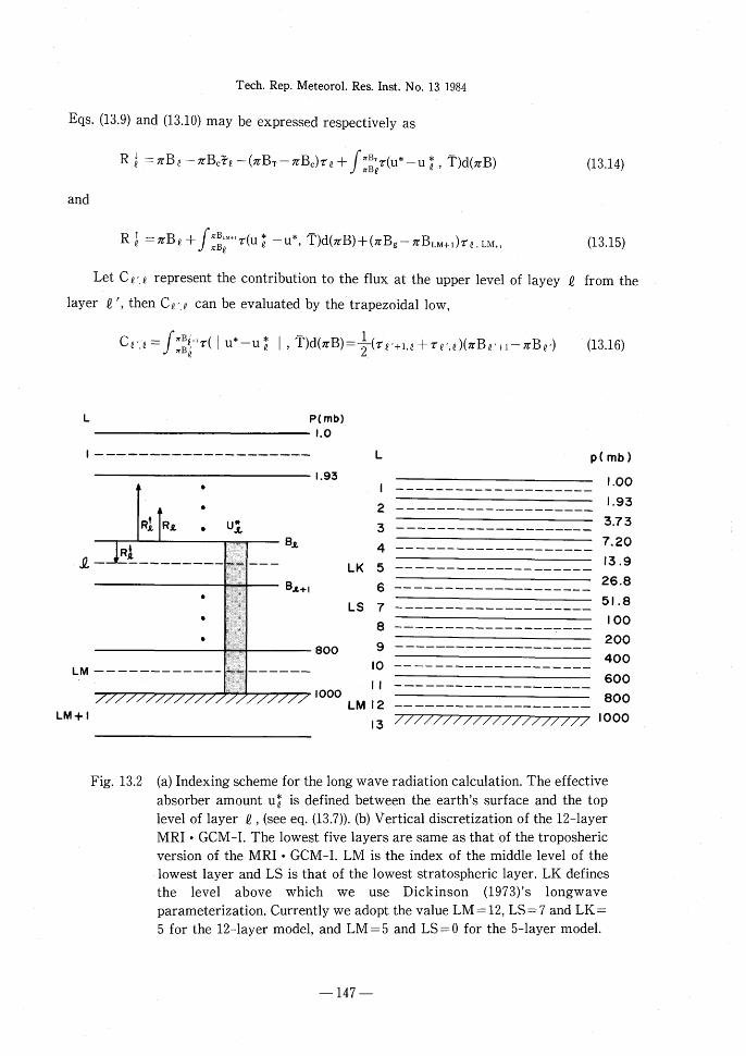
　　　The　vertical　discretization　of　the　atmosphere　and　the　vertical　index　are　shown　in　Fig．13。

2．With　use　of　the　notation

　　　　　　勤二そ2（u蕊一u育一u董，Tc）

　　　　　　　τ2二τ2（u蕊一u董，T）

　　　　　　　宛，Fτ（lu董・一u捌，T）≡τ2，2’　　　　　　　　　　　（13・13）

一146一

Tech．Rep．MeteoroL　Res．Inst．No．131984

Eqs，（13。9）and（13，10）may　be　expressed　respectively　as

Rl一πB乏一πBcそ2一（πBT一πBc）τ2＋隠τ（u＊一u育，T）d（πB） （13．14）

and

Rl一πB2＋∫霊別・τ（u童一u＊，T）d（πB）＋（πBg一πBLM＋1）τ尼，LM、1（13．15）

　　　LetCゼ．乏representthec・ntributi・nt・thefluxattheupPerlevel・flayey2

1ayer2〆，then　Cゼ，2can　be　evaluated　by　the　trapezoidal　low，

from　the

C2㌦2一焼・τ（lu＊一u言1・T）d（πB）一吉（τを・＋1，4＋τ2’，を）（πB4’＋1一πBの（13．16）

L P‘mb》

1．0

1　一一一一一一欄一聞騨一一一一噂隔噸隔一一。一一一 L1．95　　　　　　　　1

　　　　　　　2

　　　　　　　3

　　　　　　　4

　　　　LK　5

　　　　　　　6

　　　　LS　7

　　　　　　　8

800　　　9　　　　　　　10

　　　　　　　111000　　　　LM　l2

　　　　　　　13

P（mb》

ユー

LM十1

R五R£

●●●

uヱ

『

R五

一　一　｝　殉　一一一　一一鰯 蝿脚 一　一　　一

Bユ

●●●

B4＋1

一　　一　　一　　一　　一　一　一　　一　　一　　一　一　一 暴霧噸 一　一　　一　一　一　『

1．OO

l．933．7：3

7、20

13．9

26．8

51．8100

200400600800

1000

Fig．13．2 （a）Indexing　scheme　for　the　long　wave　radiation　calculation．The　effective

absorber　amomt　u肯is　defined　between　the　earth’s　surface　and　the　top

level　of　layer2，（see　eq．（13．7））．（b）Vertical　discretization　of　the12－1ayer

MRI・GCM－1．The　lowest　five　layers　are　same　as　that　of　the　troposheric

version　of　the　MRI・GCM－1．LM　is　the　index　of　the　middle　level　of　the

lowest　layer　and　LS　is　that　of　the　lowest　stratospheric　layer．LK　defines

the　level　above　which　we　use　Dickinson　（1973）’s　longwave

parameterization．Currently　we　adopt　the　value　LM＝12，LS＝7and　LK＝

5for　the12－1ayer　mode1，and　LM＝5and　LS＝O　for　the5－1ayer　mode1．

一147一

Tech．Rep。Meteoro1，Res．Inst．No．131984

1．O

oO』

トm卜

とJ讐

o購

lq

　O↑

7B一印－司

　①卜

q＋q

　　①ト

一↑畦

　　ooレ

　　噌

　　⑩誉

《。ロト》；ヨ①ド

ハ1卜

‘＊●塵コ

　1

＊⊃

ソ　←

O．O

q↑

↑d“詳

奪

1畢曜

oIl一・一

1㌦

1　＼lll曝

春1－q．撃評↓

9

司．㎝，♂

1嵐了構－豊

　　　　　ト

吋㎡ー噌〕

十　£

一τ／

　　　司．撃魂－亨

　　　　　　↑

↓．一↑ず

　　　q．～＋↓llΨ

　　　　　　↑

d．qQ

穏●U

　む

ULK管

u　＆一2

→←　　　　　→←　　　層』　　　　斎

U£一l　U亘U鯛Uユ＋2穏

U　…0　し酬＋1

　　　　　　菅

＿uFig，13．3 Schematic　representation　of　the　transmission　fmctionsτ（l　u＊一u訓，T）

　　　ナandτ互at　layer　2，

　　This　fom　is　approximately　valid　except　when21二2十1and21二2．When　the　two

layers　are　adjacent　to　each　other，τdoes　not　vary　linearly　withπB．Therefore，following

Katayama（1972），two　bulk　transmission　fmctions芳are　defined　as　follows，

　　　　　テ万…（πB2一πB2＿1）一1C2＿1，4　　　　　　　　　　　　　　　　　　　　　　　　　　　（13．17）

　　　　　そ吉≡（πB2＋1一πB2）一1C2，¢　　　　　　　　　　　　　　　　　　　　　　　　　　　　（13．18）

Fig。13．3shows　a　schematic　representation　ofτ（I　u＊一u老1，T）andそ吉．

一148一

　　　　　　　　　　　　　　　　　　　　　Tech．Rep．Meteorol．Res．Inst．No．131984

　　　Substituting（13。16），（13ユ7）and（13．18）into（13．14）and（13。15），we　obtain

　　　　　　　Rl一πBを一（πB2一πB遅一1）姦一青2，壌一2（τを’＋L2＋τを’，2一πBの

　　　　　　　　　　　　　　　一（πBLK一πBT）τLK，2一（πBT一πBc）τ2一πB，そを　　　　　　　　　　　（13．19）

and

　　　　　　　　　　　　　　　　　　　　　　　　　　　　　　　　　l　LM　　　　　　Rl一πB2＋（πBセ＋1一πB想）そ畜＋72，男＋1（τを’＋L2＋τゼ・c）（πB27＋1｝πBの

　　　　　　　　　　　　　　　十（πBg一πBLM＋1）τを，LM＋1　　　　　　　　　　　　　　　　　　　　　　　　（13。20）

Currently　LK二5and　LM＝12in　the12－L　model．Above　the　level　LK　we　use　Dickinson

（1973）’s　parameterization　of　long　wave　radiative　cooling　described　in　section13．7。In　the5・

L　model，LK＝1and　LM二5，

13．2．4　Cloudy　atmosphere

　　　Five　types　of　clouds　are　identified

currently．They　are　schematically　shown　in

Fig．13．4　and　are　classified　as　1）　clouds

associated　with　large－scale　condensation，2）

cirrus　associated　with　sub－grid・scale　deep

cumulus　convection，3）sub－grid－scale

penetrative　cumulus　convection，4）clouds

associated　with　middle　level　convection，

and　5）stratus　clouds　associated　with

supersaturation　within　the　planetary

boundary　layer．Currently　only　the　first

two　types　of　clouds　explicitly　interact　with

radiation．Clouds　are　treated　as　black　body

radiators　with　a　fractional　cloudiness　CL2

equals　to　unity，except　when　the　cloud

mbIOO

200

iil饗灘iii

400

C　l　RRUS

「、藤

O　　　　　　　O　　　　　　　O

O　　　　　　　O　　　　　　　O

6　　　　　　

8　　　　　　0

M　l　DDしE

しEVEL

STRATUS

Fig．13．4

　CLOUD

『驚蕪i

一鰹鰍槻華一〃1鰍灘

　　　　　　　　　　　　　　　／　　　　　　　　／

Various　types　of　cloudsidentified　in　the　MRI・GCM－1．

Radiatively　interactive　clouds

are　shaded．

1ayers　are　above400mb　or　colder　than－40。C。In　the　latter　case，clouds　are　considered　to　be

in　ice　phase（ガ．6．，cirrus），and　the　fractional　cloudiness　CL2is　assigned　the　value　O．5．Thus，

for　a　cloudy　atmosphere（13．19）and（13．20）are　modified　to

一149一

　　　　　　　　　　　　　　　Tech．Rep。Meteoro1．Res。Inst．No．131984

Rl＝πBを一（πBを一πB2－1）禿万（1－CL2－1）

　　　　　　　　　　　1　LK　　　　　　　　　　　　　　　2’　　　　　　　　　一万2，男一2（τ卿）（πBを’＋1一πB尼7）k＝ワー1（1－CLk）

　　　　　　　　　　　　　　　　　　　　　　　　　　　　　　　　　　　　　　　　　　　　　　　　モ　

　　　　　　　　　一〔（πBLK一πBT）τLK，セ十（πBT一πBc）τ4十πBcその　　n　（1－CLk）

　　　　　　　　　　　　　　　　　　　　　　　　　　　　　　　　　　　　　　　　　　　　　　　k＝2－1

Rl＝πBを十（πB碧＋1一πBセ）テ万（1－CLを）

　　　　　　　　　　　1　LM　　　　　　　　　　　　　　　　　　　ゼ　　　　　　　　　十一　　Σ　（τゼ＋1．2十τゼ，2）（πBゼ＋1一πBゼ’）H（1－CLk）　　　　　　　　　　　2を’＝セ＋l　　　　　　　　　　k一を

　　　　　　　　　　　　　　　　　　　　　　　　　　　　　モ　

　　　　　　　　　十（πBg一πBLM＋1）τを，LM＋1H（1－CLk）

　　　　　　　　　　　　　　　　　　　　　　　　　　　　k＝2

（13．21）

（13．22）

13．2．5　Effective　absorber　amounts

13．2．5．a　Water　vapor

　　　The　effective　absorber　amomt　u＊is　given　by（13．7）．The　water　vapor　mixing　ratio　qH、

o（p）is　a　prognostic　variable　which　is　calculated　by　the　way　described　in　Chapters6，7and

9，Pressure　scaling　lows　were　originally　incorpolated　to　replace　an　inhomogeneous　optical

path　with　an　equivalent　homogeneous　optical　path．Since　this　is　an　empirical　method，there

is　some　uncertainty　in　the　value　of　the　pressure　scaling　factorαH、o．In　Table13。1the　values

ofαH、o　which　is　adopted　by　various　authors　are　tabulated．CurrentlyαH，o　is　assumed　to　be

O．9atter　McClatchey8厩1．（1972），who　found　a　best　fit　to　laboratory　and　theoretical　data　for

that　value．

　　　　　　　Table13．1　Pressure　scaling　factor　for　water　vapor　adopted　by　various　authors．

MANABE6渉α乙　　　（1967）

SASAMORI　　（1968）

KATAYAMA　　（1972）

McCLATCHEY6厩乙　　　　（1972）

αH200．7 1．0 0．6 0．9

13．2．5．b　　Carbon　dioxide

　　　For　carbon　dioxide，（13．7）is　slightly　modified　as

　　　　　　　u・cα（P）一gρCま．NTP∫ISqcα（び）（妾）αc窃dび

whereρco，，NTp＝1．977kg　m－3is　the　carbon　dioxide　density　at　NTP。

　　　　　　　　　　　　　（13．23）

The　mixing　ratio　of　CO2

一150一

Tech。Rep．Meteorol．Res。Inst．No．131984

is　assumed　to　be　constant　both　in　space　and　time，and　is　assigned　the　value　O．0489percent　by

weight（qco，＝4．89x10－4），or　O．032percent　by　volume（320PPM）．Thus

　　　　　　　u・cα（P）一α黒1〔（髭）　＋1一（黄）　＋1〕　　　　（1324）

Following　Manabe　and　M611er（1961），αco，is　taken　as　O．86．

13．2．5．c　　Ozone

　　　The　ozone　mixing　ratio　qo，（p）is　predicted　in　a　way　described　in　Chapters6and12。The

predicted　amomt　is　used　for　the　radiation　calculation．The　effective　absorber　amomt　of

ozone　is　also　given　by（13．23）by　replcingρco，．NTp　andαco，withρo、、．NTp二2．144kgm－3andαo、；

0．3respectively，after　Manabe　and　M611er（1961）．

　　　Thus，

　　　　　　u・鴨．INTP，署，qq・4111＋’（妾）α・・d・　　　　（1325）

13．2．6　Empirical　transmission　function　equations

13．2．6．a　Water　vapor

　　　Total　transmission　function　of　a　mixture　of　gases　is　given　by（13．11）and（13．12）．

Yamamoto（1952）calculatedτandそfor　water　vapor　from　experimental　laboratory　data．

Katayama（1972）obtained　the　empirical　transmission　functions　forτH，o（u斉，o，T）by　taking　an

average　ofτgiven　by　Yamamoto（1952）for　T二220。K，260。K，and300。K，乞．ε．，

一・T・一灘鎌蹄＜1・’、13，6）

where　F（a，b）＝1／（1十au＊b）and　Z二10910u＊．

And　for商，o（u＊，Tc）

一K・一／l欝lll讐腿＜α1）（、a，，、

13．2．6乙b　　Carbon　dioxi－e　an《l　ozone

　　　We　adopt　empirical　transmission　function　equations　derived　by　Schlesinger（1976）both

for15μband　of　carbon　dioxide　and　for9。6μband　of　ozone　based　on　the　experimenta1

一151一

Tech．Rep，MeteoroL　Res．Inst．No。131984

1aboratory　measurements　by　Elsasser（1960）．

　　　　　　τco，（uさo，，T）＝0．924－0．0390Z－0．00466Z2　　　　　　　　　　　　　　　　　　（13．28）

　　　　　　τo、（uδ、，T）　＝0．919－0，0252Z－0。000998Z2　　　　　　　　　　　　　　　　　　（13．29）

where　Z　equals　to　loglouδo、for（1328）and　logユouδ、for（13．29）．τco，（uδo，，T）andτo，（uδ、，T）are

defined　as　the　arithmetic　mean　ofτco，andτo、over－80。C　to400C．

13．2．6．c　　Bulk　transmission　functions

　　　Katayama（1972）introduced　the　bulk　transmission　fmctions葦by（13，17）and（13ユ8）

which　are　evaluated　by　linear　interpolation　between鷲＝1fo対u＊一u割二〇and鷲＝商±1，セ

as，

　　　　　　荒二（1十m吉劾±1，2）／（1十m吉）　　　　　　　　　　　　　　　　　　　（13．30）

　　　Thelinearinterpolationfactorsm吉mustbedeterminedbythephysicalparametersof

the　adjacent　layers．Katayama（1972）determined　m吉　once　and　for　all　by　numerical

experiments　in　which　trapezoidal　integration　scheme（13．17）was　evaluated　numerically　by

subdividing　the　layer　under　consideration　into　thin　sublayers　of10mb　thickness．In　this

calculation，the　vertical　distribution　of　the　water　vapor　mixing　ratio　q　and　the　temperature

T　in　an　adjacent　layer　are　assumed　to　be

　　　　　　q二q2（P／P2）k2　　　　　　　　　　　　　　　　　　　　　　　　　　　　　　　　　　　　　（13．31）

　　　　　　T＝T2十γパP－P2）

　　　We　follow　Katayama／s（1972）numerical　experiment．He　could　express　m吉

approximately　as　a　linear　function　of△p，the　depth　of　layer　in　mb，when　the　remaining

parameters　are　fixed。Thus，

　　　　　　m吉＝a去十b吉△p／100。　，　　　　　　　　　　　　　　　　　　（13．32）

　　　a吉and　b吉are　obtained　empirically，

a亥＝L吉（Pゼ）十F吉（z2）

（13．33）

　　　　　　b古一L志（P，）＋F志（z，）＋（言1）＋△k2＋（諜）＋△γ4

where△k二k2－3，△γセ＝γ慈一10（。K／100mb），and

　　　　　　L右（Pを）＝一1．66十1．7610910Pを，

　　　　　　L右（P2）＝一〇。197十〇．0002P2，

　　　　　　F吉（Z4）＝0．30Z2十〇．28Zう十〇．04Z亀，

　　　　　　Fも（Z君）＝0．0812Z1－0．045Zぞ十〇．02334Z駐，

（13．34）

（13．35）

一152一

Tech．Rep．Meteorol．Res．Inst．No．131984

　　　　　　　（諜）＋一Min（一・．・41＋・。・21Z2，『・．・・6）く・，

　　　　　　　　　　　　　　　　　　　　　　　　　　　　　　　　　　　　　　　　　　　　　　　　　　　　　　　　　　　　　　　　　　　（13．36）

　　　　　　　（霧）＋一Max（…1225＋・…7Z2，・。・・93）〉・，

　　　　　　　a万＝一〇・OgL石（Pを）十F右（z2－0・105L互（P2）），　　　　　　　　　　　　　　　　　　　　　　（13．37）

　　　　　　　b万一一…9L巧（P2）＋Fも（Z2一・・1・5L石（Pを））＋（蝶）一△k2＋（鉾）一△γ2

　　　　　　　L石（p2）＝Max（61．86－22．9210910p2，76。63－28．391091。pを），　　　　　　　　（13．38）

　　　　　　　L君（pを）＝Min（一42．59十15．7810910pを，一60．81十22。531091。pゼ），

　　　　　　　FE（X）二2．57＋0233X＋0．18×2＋0．027×3，　　　　　　　（13．3◎）

　　　　　　　Fも（X）＝1．42十〇．48X十〇．16×2十〇．011×3，

　　　　　　　（蝶）一一・，・8＋（・。371一・．1・21・91。Pを）（zセ＋2ユ）＞・，

　　　　　　　　　　　　　　　　　　　　　　　　　　　　　　　　　　　　　　　　　　　　　　　　　　　　　　　　　　　　　　　　　　　（13．40）

　　　　　　　（霧）一一Min（一・。・325一・．・・5z2，一・。・275）＜・，

In　the　above　Z2＝10910qを，Z1＝l　Zセ十2．51，and　X　is　a　dummy　variable．

　　　Recall　that芳were　introduced　due　to　the　failure　of　the　trapezoidal　integration　scheme

for　the　layers　adjacent　to　the　level　mder　consideration．τvaries　more　rapidly　withπB　than

a　linear　relationship　within　these　layers．This　nonlinear　character　ofτis　most　pronomced　in

the　troposhere　where　water　vapor　is　abundant．However　in　the　stratosphere　where　water

vapor　is　less　impotant，πB　is　more　miform（Schlesinger，1976）．Thus，

　　　　　　　m吉＝1　　　　　　　　2＜LS　　　　　　　　　　　　　　　　　　　　　　　　　　　　　　　　　　　　　　（13．41）

is　assumed　above　lOO　mb　leveL

13．2．7　Long　wave　radiative　cooling　in　the　upper　stratoshere

　　　Although　Katayama’＄method　of　using　mean　transmission　functions（13．5）and（13。6）is

good　in　the　troposhere　and　also　in　the　lower　stratoshere，it　is　less　so　in　the　upper　stratosphere

where　misotropy　of　radiative　flux　dominates．As　a　substitute　of　Katayamals　method，we

adopt　Dickinson（1973）ノs　long　wave　radiative　cooling　parameterization　in　the　upper

stratoshere（乞．6．the　region　above13．9mb　in　the　current121ayer　version．See　Fig。13．2）。

That　is

　　　　　　　（票）t，一一C・，ゼーa・，2（T2－T・，2）β2　　　　　　（13・42）

153一

Tech．Rep。Meteorol．Res。Inst，No．131984

where

β2＝

1，

1十0．0033（T2－T。、を）

96。e－96・／T・，2（丁乏一丁．，乏）Tl・を

　　　　T。，2－135

e－960／T4＿e－960／To・を

ifI　Tを一丁。，4『＜50K

　　if　l　T－T。，¢1＞5。K　and　T坦〉130。K

ifl　T2－T。．乏1＞5。KandT2＜130。K

（13．43）

C・，をisthec・・1ingrateexpe6tedf・rthereferencetemperaturepr・fileT．，2，anda．，2isa

Newt・nianc・・1ingc・efficient・Asf・rareferencetemperatureT・，2，the1962standard

atmosphere　profile　is　adopted．β建is　a　modification　factor　introduced　by　Dickinson　and

revised　by　Schlesinger（1976）．

　　　The　values　of　T。1を，C。．2and　a。．セfor　the　upper　four　layers　are　presented　in　Table13．2．

Table13．2　Values　used　in　the　Dickinson’s　long　wave　cooling　parameterization．

kP 丁曜 C曜 ao，2

（mb） （K） （K　DAY－1） （DAY－1）

1 1．39 265．73 9．47 0，180

2 2．68 251．81 6．14 0，127

3 5．18 238．57 4．17 0．0993

4 10．0 227．72 2．62 0．0755

13．3　　Solar　radiation

13．3．1　　Basic　quantities

　　　The　extraterrestrial　solar　flux　incident　on　a　horizontal　surface　is　given　by

　　　　　　　S－S。（塵）2c・sζ　．　　　　　　　　　　　（13・44）　　　　　　　　　　　　　γE

where

　　　　　　　c・sζ＝sinφsinδ＋c・sφc・sδc・sh，　　　　　　　　　（13・45）

S。＝1345watt　m－2is　the　solar　constant　at　one　astronomical　unitγE，γE　is　the　earth－sun

distance，ζisthes・1arzenithangle，φisthelatitude，δisthes・lardeclinati・nandhisthe

hour　angle　of　the　sm．As　shown　in　Appendix　A13ユ，δandγE　can　be　determined　by　a

perturbation　of　Kepler〆s　second　low．The　hour　angle　at　each　grid　point　is　updated　at　every

一154一

Tech．Rep．MeteoroL　Res．Inst．No，131984

diabatic　time　step，and　the　solar　declination　and　earth－sun　distance　are　updated　once　a

simulated　day．

　　　In　the　solar　radiation　parameterization　developed　by　Katayama（1972）and　Schlesinger

（1976），the　solar　flux　under　cloudless　conditions　is　depleted　only　by　water　vapor　and　ozone

absorptionand　Rayleigh　scattering．The　effective　absorption　bands　of　water　vapor　for　the

solar　spectrum　exist　in　the　wave　length　rangeλ＞0．9μ．As　the　amount　of　Rayleigh　scattering

varies　asλ一4，the　scattering　in　that　range　can　be　neglected．As　for　ozone，the　absorption

bands　exist　in　the　wavelength　rangeλ＜0．8μ．Because　the　amomt　of　Rayleigh　scattering

increases　exponentially　with　pressure，and　because　the　heatingby　ozone　absorption　below200

mb　is　negligible　compared　to　the　heating　by　water　vapor　absorption，we　can　neglect　the　effect

of　Rayleigh　scattering　on　ozone　absorption　above200mb　and　also　neglect　the　effect　of　ozone

absorption　on　Rayleigh　scattering　below200mb．

　　　Following　Joseph（1966，70）and　based　upon　above　considerations，the　solar　radiation　is

divided　into　two　parts．One　isくてthe　scattered　part”，

　　　　　　　S8＝0．634S。cosζ　　　　　　　0．9μ＞λ　　　　　　　　　　　　　　　　　　　　　　　　　　（13．46）

and　the　other璽疋the　absorbed　part”，

　　　　　　　S8＝0．366S。cosζ’　　　　　　　λ＞0．9μ　　　　　　　　　　　　　　　　　　　　　　　　　　（13．47）

13．3．2　Absorptivity　of　water　vapor

　　　Schlesinger（1976）calculated　water　vapor　absorptivity　AH，o　from　the　data　ofMcClatchey

6渉σ1．（1972）and　approximated　the　absorptivity　piecewisely　by　quadratic　polynomials；

　　　　　　　A／H，o（X）　二趣十bX十qX2　　　　　Xガー、＜X＜Xガ　　　　　　　　　　　　　（13・48）

　　　　　　　AH，o（X）　二A’H，o（X）／0．366　　　　　　　　　　　　　　　　　　　　　　　　　　（13・49）

　　　　　　　X二u＊M　　　　　　　　　　　　　　　　　　　　　　　　　　　　　　（13．50）

where　the　effective　water　vapor　amomt　u＊is　given　by（13。7），

　　　　　　　M＝35secζ／　　　　　　　　　　　　　　　　　　　　（13。51）

is　the　magnification　factor　after　Rodgers（1967），with　sphericity．AH，o（X）is　the　absorptivity

for　the《更absorbed”part，and　A〆H，o（X）is　the　absorptivity　for　the　total　solar　spectrum．The

coefficients　aげ，bε，and　cεare　presented　in　Appedix　A132．

　　　By　letting　y＝A〆H，o（X），the　inverse　function　X二A’一1H、o（y）was　fitted　into　quadratic

polynomialsl

　　　　　　　X二A－1H、o（y）＝dj十ejy十fjy2，　　　yj－1〈y＜yj　　　　　　　　　　　　　　　　　（13・52）

一155

　　　　　　　　　　　　　　　　　　Tech．Re登．Meteorol．Res．Inst。No。131984

The　coefficients　dj，ej，and　fj　are　also　presented　in　Appendix　A13．2．

13．3．3　Absorptivity　of　ozone

　　　The　absorptivity　fmction　of　ozone　for　the　total　solar　spectmm　was　calculated　by

Schlesinger（1976）and　was　fitted　by　quadratic　polynomialsl

　　　　　　　Alo，（X）二aゴ十b∫X十qX2　　　　　XH＜X＜Xε　　　　　　　　　　　　　　（13．53）

　　　　　　　Ao、（X）　二A〆o、（X）／0．634　　　　　　　　　　　　　　　　　　　　　　　　　　　　（13．54）

where　Ao、（X）is　absorptivity　for　theヒ聖scattered”part，A〆o、（X）is　the　absorptivity　for　the　entire

solar　spectrum　and

　　　　　　　X＝uδ，M

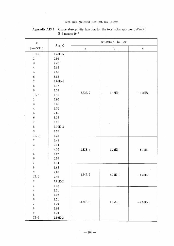
The　coefficients　aj，bj，and　c」are　tabulat6d　in　Appendix　A13．3。

　　　The　effective　ozone　amomt　uδ，is　calculated　by，（cf．eq。（13．21））

　　　　　　　u義一ρ．素TP∫1ρq（z）dz－gρ．INT，∫IPα（P・）dび　　　　（13・55）

whereρo、is　the　ozone　density，qo、is　the　ozone　mixing　ratio　andρo、．NTp二2．144kg　m－3is　the

ozone　density　at　NTP，In　a　discrete　case，（13．55）can　be　written　as，

　　　　　　　　＊　　　　1　　珍　　　　　　　uo、，2十　　　Σqo，。ゼ（pゼ＋1－pの　　　　　 ‘　　　　　　　　　　（13．56）　　　　　　　　　　　　9ρ03，NTPゼ＝1

where　pを，is　the　pressure　at　the　upper　surface　of　layer2’，qo，，ゼthe　predicted　ozone　mixing

ratio　for　layer　2’，and

　　　　　　　u＆，を一ρ．3㌔TP∫1，渇ρ・・（z）dz　　　　　　　（13・57）

Incalculating（13．57），weassumethat・z・nenumberdensityn・、（z）ab・vethet・plevel・fthe

m。delz。．5decaysexp・nentiallywithaltitudef・ll・wingthemean・z・nedistributi・nby

Krueger（1973）．Thus，

　　　　　　　　nδ，（z）一n・、（z・）exp（z看z1）z≧z・　　　　　　（13・58）

whereZ、isthealtitude・fthemidleve1・flayer1，andH－4・35km・Sub5tituting（13・58）int・

　（13．57）gives

　　　　　　　　　　　　　　　　　　Hexp（一zo・5責z1）q・・，2P1．5

　　　　　　　　　＊　　　　　　　　　　　　　　　　　　　　　　　（13。59）　　　　　　　　Uo3・2一　　　　　　　　ρo，，NTpRTl

Wherep、．5andT、arepressureandtemperatureatthemidleヤe1・flayerlrespectively，and

一156一

Tech．Rep．Meteorol．Res．Inst．No．131984

Risgasconstant．

13．3．4　Clouαless　atmosPhere

13．3．4．a　般Absorbed”part

　　　The璽でabsorbed”part　of　the　solar　radiation　S言is　absorbed　only　by　the　water　vapor　in　the

troposhere　and　at　the　earth〆s　surface．The　other　absorption　canbe　neglected．（6．g．The　absorption

by　the　water　vapor　in　the　stratoshere　can　be　neglected　in　comparison　to　the《更scattered”part

absorption　by　ozone．）

　　　After　neglecting　the　absorption　by　water　vapor　on　the　radiation　reflected　by　the

earth’s　surface，the　net　downward　flux　of　the《史absorbed”part　at　the　upper　surface　of　layer

2，Sa，ゼ，is

　　　　　　　Sa，2二S3　　　　　　　2＝1，……，LS　　　　　　　　　　　　　　　　　　　　　　　　　　　　（13．60）

　　　　　　　Sa，2＝Sa｛1－AH、o〔（u査，o，。。一u斉，o，を）M〕／　　2＝LS十1，……，LM十1

where　AH，o　was　given　by（13．48）and（13．49）．The　absorption　of　solar　radiation　by　water　vapor

in　layer2，ASa，珍，is　therefore

　　　　　　　ASa，を＝0．0，　　　　　　　　　　　　　　　2＝1，……，LS　　　　　　　　　　　　　　　　　　　　　　　　　　　　　　　　　　　　　　　　　　　　　　　　　　　　　　　　　　　　　　　　　　　　　（13．61）

　　　　　　　ASa，乏＝Sa，2－Sa，を＋1，　　　　　　　　　2＝LS十1，……，LM

　　　The　absorption　of　the　solar　radiation　that　is　absorbed　at　the　earth〆s　surface　is

　　　　　　　ASa，LM＋1＝（1一α，）Sa，LM＋1　　　　　　　　　　　　　　　　　　　　　　　　　　　　（13．62）

whereαs　is　the　albedo　of　the　surface，which　is　given　in　Table13．3．

13．3．4．b　駅Scattered”part

　　　By　neglecting　the　effect　of　Rayleigh　scattering　on　ozone　absorption　above200mb，the

downward　flux　and　the　absorption　of　the　downward　flux　of　the　scattered　part　are

　　　　　　　S論二S8／1－Ao、（uδ，，セM）／　　　　　　　　　　　　　　　　　　　　　　（13。63）

　　　　　　　AS論＝S論一S論＋1　　，　2二1，……，LS十1

　　　　　　　AS“二〇．0　　　　　　，2二LS十2，一・・，LM　　　　　　　　　　　　　（13．64）

where　the　effective　ozone　amomt　uδ、，を，is　given　by（13。56）and（13。59）。

　　　By　neglecting　the　effect　of　ozone　absorption　on　Rayleigh　scattering　below200mb，the

downward　flux　of　the曜璽scattered”part　at　the　earth’s　surface，S議M＋1is

　　　　　　　Ss，LM＋1＝SよLs＋2（1一α。）／（1一α。α，）　　　　　　　　　　　　　　　　　　　　　　　　　　　　　　　　（13・65）

where

一157一

Tech．Rep。Meteorol．Res。Inst．No．131984

Table13．3Surface　albedo　adopted　in　the　MRI・GCM－1

Surface　condition Albedo

open　ocean 0．07

bare　land 0．14

frozen　land 0．3

permanent　land　ice　and　snow Min（0。85，0。7十〇．15h）where　h　is

height　in　km

bare　sea　ice 0．4

SnOW　On　Sea　iCe 0．7

meltingもnow 0．5

α・一…85一・2471・91・（品・sζ）（13．66）

is　the　albedo　due　to　Rayleigh　scattering．（Coulson，1959）

　　　　The更璽scattered”part　of　the　solar　radiation　that　is　absorbed　at　the　earth’s　surface　is

　　　　　　　AS，l　LM＋1＝（1一αs）SslLM＋1　　　　　　　　　　　　　　　　　　　　　　　　　　　（13．67）

The　upward　flux　of　the璽《scattered”part　at　LS十2，S試Ls＋2，is

　　　　　　　S，ILs＋2　　＝SまLs＋2－ASslLM＋1

　　　　　　　　　　　　　　　　二SまLs＋2｛1一（1一α，）（1一α。）／（1一α。αs）／　　　　　　（13．68）

By　neglecting　the　effect　of　Rayleigh　scattering　on　ozone　absorption　above200mb，the

absorption　of　upward　flux　of　theヒ更scattered”part　in　layer2，AS、，2is

　　　　　　　AS藁二S、ILs＋2／Ao，〔uδ、，Ls＋2M十1．9（uδ，，Ls＋2－uδ、，2）〕

　　　　　　　　　　　　　　　　一Ao、〔uδ、，Ls＋2M十1。9（uδ、，Ls＋2－uδ，，2＋1）〕｝，2二1，……，LS十1

　　　　　　　　　　　　　　　　　　　　　　　　　　　　　　　　　　　　　　　　　　　　　　　　　　　　　　　　　　　　　　　　　　　　　（13．69）

　　　　　　　ASsl4＝0．0　　，2＝LS十2，……，LM

where　the　factor1。9is　an　average　magnification　factor　for　the　diffuse　upward　radiation．

（Lacis　and　Hansen，1974）

　　　The　heating　rate　due　to　absorption　of　solar　radiation　at　layer2　is　given　by

　　　　　　　（誓），蔦、一9（AS譜誓会S』）　　　　　（13．7・）

where　p2is　the　pressure　at　the　upper　surface　of　Iayer2．（（ヅ．（13．4））

一158一

Tech．Rep．Met∈oroL　Res．Inst．No．131984

13．3．5　Cloudy　atmosphere

13．3。5．a　Single　cloud

　　　Consider　a　single　cloud　located　in　layer

L　as　shown　in　Fig．13．5．The　flux　of　the

虻史absorbed”　part　at　the　upPer　surface　of

layer　2＜L，Sa，2，is　given　by（13．60）as

　　Sa，乏二S3／1－AH，o〔（u査，o，。。一蜻，o，2）M〕／

　　　　　　　　　　　　　　　　　　　　　　　　　　　　（13．71）

By　letting　Ac，L　and　R，，L　denote　the

absorptivity　per　unit　pressure　thickness

and　the　reflectivity　of　cloud　layer　L，the

flux　of　the　奴absorbed”　part　at　the　upPer

surface　of　layer　L十1，S、，L＋1，is　given　by

　　　　　　　Sa，L＋1＝〔1－Rc，L－Ac，L（PL＋rpL）〕Sa，L

S・，LU篇2・，し

Ac，LI，Rc，u，Rを，u一一一

So，L†1

PL

Fig．13．5

Pし＋1

L

uも5，L

where　the　quantity　in　brackets　represents　the　transmissivity　of　cloud　layer．L。

calculate　the　fluxes　beneath　the　cloud　by（13．71），the　total　optical　thickness　from　the　top　of

the　atmosphere　to　the　upper　surface　of　the　layer　mder　consideration　is　required．Katayama

（1972）defined　the　equivalent　total　optical　thickness　of　water　vapor　from　the　top　of　the

atmosphere　to　the　base　of　the　cloud　layer　L，TL＋1，by

　　　　　　　（1－Rc，L）S3｛1－AH，o（rL＋1）｝＝Sa，L＋1，　　　　　　　　　　　　　　　　　　　　　（13．73）

hence

　　　　　　　で・＋・一A百お（1一（1§憲ll）S3）　　　　　　（13・74）

where　A苗o　is　the　inverse　of　the　water　wapor　absorbtivity　fmction　given　by（13。52）。The　flux

across　the　upPer　surface　of　any　layer　beneath　the　cloud　base　is，then，given　by

　　　　　　　Sa，2＝（1－Rc，L）S3｛1－AH，o〔rL＋、十1。66（婿、o，L＋1－u査，o，£）〕｝　　　　　　　　　　（13．75）

where1。66is　the　diffusivity　factor　for　diffuse　radiation　beneath　the　cloud．The　absorption　of

solar　radiation　is

Asinglecloudlayer．u斉，o，2follows　the　definition　of　eq．（13．

7），while　u査，o，E　defined　as　the

effective　ozone　absorber　amount

between　the　bottom　level　of

layer2　and　　top　　of　　the

atmosphere．

　　　　　　　　　　　　　　　　　　　　　（13．72）

　　　　　　　　　　　　　　　　　　　In　order　to

　　　　　　　AS乱・一｛注“1－SIL＋儒＋1’”””’LMeXcept2＝L　（13・76）

whereRgListhereflectivity・fc1・udlayeτLf・rthe聖促abso「bed”pa「t，andSa・L・thesola「

radiations　reflected　from　the　cloud　layer．The　absorption　of　radiation　reflected　from　the

一159一

　　　　　　　　　　　　　　　　　　　　　　Tech．Rep。Meteorol．Res．Inst．No．131984

cloud　layer　is　neglected．The《虻absorbed”part　of　the　solar　radiation　that　is　absorbed　at　the

earth’s　surface　is　given　by（13．62）．

　　　In　the　case　of敗scattered”part　of　the　solar　radiation，equations（13．63），（13。64），（13．67），and

（13．69）are　unchanged．In　equations（13．65）and（13．68），α。is　replaced　byα，，the　albedo　of　the

cloudy　atmosphere　for　the更｛scattered”part，

　　　　　　　αc＝1一（1－R∈，L）（1一α。）　　　　　　　　　　　　　　　　　　　　　　　　　　　　　　　　（13．77）

where　R∈，L　is　the　reflectivity　of　cloud　layer　L　for　the《虻scattered”part．

13．3．5．b　Two　or　more　contiguous　clouαlayers，and　multiple　clouds

　　　In　the　mode1，each　cloud　layer　within　two　or　more　contiguous　cloud　layers　is　treated　as

a　separate　cloud　for　the　solar　radiation　calculation　like　one　of　multiple　clouds．

　　（A）　《《Absorbed”part

　　　Forsimplicity，considertwocloudseach　　　　　　　　　　　　　　　　　　　　　　　　　　　　　　　　　　　　　　　　　　　　　　　　　　　　　　　So，u

c。nsisting。fasinglelayer。Thecl。udllies　　　　　　　　　pLl

inthelayerLlandthecl・ud2inthelayer一一一Ac，Ll百c，Ll一一一一一歳，Lr一一一¢一LI

L2（see　Fig．13。6）．For　layers2＜Ll，S、，2is

givenby（13．60），　　　　　　　　　　　　S　　　　pu＋1　　　　　　　　　　　　　　　　　　　　　　　　　　　　　　　　　　　　　　　　　　　　　　　　　　　　　　　　0，U＋口

　　　　　　　Sa，2＝S葛｛1－AH，o〔（u蓋、o，。。一u斉，o，2）　　　　　　　　　　　　．

M〕｝　　　　　　　　　　　　　　　　　　　　　　　　　　●　　　　　　　　　　　　　　　　　　　　　　　　　　　　　　　　　　　　　　　　　　　　　　　　　　　　　　

　　　　2＝LS十1，一一，LM十1　　　（13．78）　　　　　　　　　　　　S　　　　　　　　　　　　　　　　　　　　　　　　　　　　　　　　　　　　　　　　　　　　　　　　　　　　　　　　o，し2　　　　　　　　　　　　　　　　　　　　　　　　　　　　　　　　　　　　　　　　　　　　　　　　　　　　　　　　　　　　　　　　　　　　　　PL2

By（13．72），Sa，Ll＋1is

　　　　　　　Sa・L1＋1＝〔1－Rc・L1－Ac・L1（PL・＋1一　　一一一Ac，L2再c，L2一一一一一百13L2一一一一£昌L2

PL1）〕Sa，Ll　　　　　　　　　　　　　　　　　　（13．79）

　　　　　　　　　　　　　　　　　　　　　　　　　　　　　　　　　　　　　　　　　　　　　　　　　　　　　　　　　　　　　　　　　　　　　　PL2＋l

By　（13．74），the　equivalent　total　optical　　　　　　　　　　　　　　S　　　　　　　　　　　　　　　　　　　　　　　　　　　　　　　　　　　　　　　　　　　　　　　　　　　　　　　　q，L2＋l

thickness　from　the　top　of　the　atmosphere

t。thebase。fc1。udl，rL、，is　　　　Fig・13・6Tw・separatedcl・udlayers・

　　　　　　　rL1－A百お（！一（1曇養嵩S3）

　　　　　　　　　　　　　　　　　　　　　　　　　　　　　　　　　　　　　　　　　　　　　　　　　　　　　　　　　　　　　　　　　　　　　（13．80）

The　flux　across　the　upper　surface　of　layers　L1十2＜2＜L2is　given　by（13．75）

　　　Sa，2＝（1－Rc，1）S3AH，o〔1一｛FL1十1。66（u斉，o，L1＋1－u斉，o，を）／〕

S、．L2＋l　is　given　by

　　　Sa，L2＋1＝〔1－Rc．L2－Ac，L2（pl．2｝1－pl、2）〕Sa，L2

（13．81）

（13．82）

一160一

　　　　　　　　　　　　　　　　　　　　　　Tech，Rep．Meteoro1。Res．Inst，No．131984

where　use　has　been　made　of（13．72）。The　equivalent　total　optical　thickness　from　the　top　of　the

atmosphere　to　the　base　of　cloud2，rL2，is

r・・一酬1一（（1－R、llll署Rq2）S3）｝　　　　　（13・83）

The　solar　flux　incident　on　the　lower　cloud2，S、，L、，is　affected　by　the　existence　of　cloud　l（see

（13．79））．Then，from（13．82）and（13．83〉ノTL2differs　from　what　it　would　be　if　cloud　l　did　not

exist；that　is，the　equivalent　total　optical　thickness　is　a　function　of　the　overlying　cloud　cover．

The　flux　across　the　upper　surface　of　layers2＞L2十2is

　　　　　　　Sa，2＝（1－Rc，2）（1－Rc，1）S琶｛1－AH，o〔～L2十L66（u芒2＋ru畜）〕／

　　　　　　　　　　　　　　　　　　　　　　　　　　　　　　　　2＝L2十2，……，LM十1　　　　　　　　　　（13．84）

The　absorption　of　solar　radiation，ASを，is

A亀・憶』一鉱騒L臨躍　・・3…

The　direct　solar　radiation　in　the史更absorbed”part　that　reaches　the　earth’s　surface，Sl，LM＋1is

　　　　　　　Sl，LM＋1二（1－Rc，2）（1－Rc，1）S3／1－AH，o〔rL2十1．66u斉，o，L2＋1〕｝　　　　　　　　　　（13．86）

The　indirect　solar　radiation　in　the《更absorbed”part　that　reaches　the　earth／s　surface　due　to

multiple　reflections　between　the　two　clouds，Sl，LM＋1，is

　　　　　　　S乱LM＋1一（Rg2S亀L2）（1一餐llRq2〉（1－Rら2）（1一訟g、2）　　　（13・87）

　　　　　　　Rq、，，一1一（（1－Rq2（1；Rら2））　　　　　　　　（・3．88）　　　　　　　　　　　　　　　　　　　　1－Rc，王Rc，2

is　the　albedo　of　the　two　clouds（neglecting　atmospheric　absorption　of　the　reflected　radiation）．

The　total　solar　radiation　in　theく疋absorbed”part　reaching　the　earth’s　surface　Sa，LM＋1，is

　　　　　　　S、，LM＋1＝Sl，LM＋1＋Sl，LM＋1　　　　　　　　　　　　　（13。89）

and　the　absorption　by　the　earth’s　surface　is　given　by（13．62）。

　　　The　above　equations　may　be　generalized　in　a　straightforward　mamer　to　the　case　of　an

arbitary　number　of　cloud　layers．

　　（B）　く更Scatterd”part

　　　The　treatment　is　the　same　as　that　described　in　subsection13．3。5but　Rε，L　in（13．77）is

replaced　by　Rε，1，2which　is　given　by（13，88）with　Rc，」replaced　by　R∈，」．

一161一

Tech．Rep．MeteoroL　Res，Inst。No．131984

13．3．6　The　reflectivity　and　absorptivity　of　clouds

　　　The　reflectivities　of　the史でabsorbed”part　Rc，and　that　of　the《璽scattered”part　Rε，and　the

absorptivity　per　unit　pressure　thickness　of　the《更absorbed”part　Ac，and　that　of　the《《scattered’7

part　Aε，for　cloud　layer　are　assumed　to　be　characterized　by　the　respective　properties　of　low，

middle，or　high　clouds　following　Rodgers（1967）and　Katayama（1972）．That　is

瓦・・R敏・）一鷹i騰ill　llil蕪、黙・一

歳・一魂iil熱il糀蕪、欝

where　p2is　the　pressure　of　the　upper　surface　of　layer2．

Appendix　A13．1Calculation　of　earth・sun　distance　and　solar　zenith　angle

A13．1．1　Earth．sun　distance

　　　Although　the　earth〆s　orbit　around　the　sun　is　elliptic，the　eccentricity　of　the　earth〆s　orbit

is　so　sma11（e二〇．Ol672）that　the　orbit　is　in　fact　very　nearly　circular．Therefore　the　earth・sun

distanceγE　and　the　angular　position　of　the　sunω（t）can　be　expressed　as　an　asymptotic　series

in　terms　of　mean　angular　position　M（t）measured　by　a　constant　angular　velocity　with　the

periodicity　of　one　year，

　　　　　　　　　　　　2π

　　　　　　　M（t）＝T（t－t・）・　　　　　　　　　　　　（A13・1・1）

where　T　is365days，t。the　time　of　perigee．The　date　of　perigee　adopted　in　the　MRI・GCM－

I　is　January3。36which　is　the　mean　date　of　perigee　from　l950through1972．Therefore，M（t）

is　expressed　as

　　　　　　　M（t）二〇．Ol72142（t－2。36），　　　　　　　　　　　　　　　　　　　　　（A13．1．2）

where　t　is　th6time　in　days　counted　from　January1．Then，from　Kepler’s　second　low

　　　　　　　　　γE（t）／γE＝Ao－AI　cosM－A2cos2M－A3cos3M一……，　　　　　　（Al3．1．3）

　　　　　　　　　　　　ω（t）二M十BIsinM十B2sin2M十B3sin3M十……，

where　　　　　Ao＝1十e2＝1．00027956，

　　　　　　　　　　　　　A1＝e－e3－e5一……駕0．01671825，

　　　　　　　　　　　　　A2＝e2－e4一……　　駕0．00013975，

一162一

Tech．Rep．MeteoroL　Res。Inst．No．131984

　　　　　　A3ニe3－e5一……

　　　　　　B1＝2e－e3十e5一……

　　　　　　B2＝e2－e4十……

　　　　　　B3＝e3－e5十……

andγE　is　one　astronomical　mit．

窄0・00000175・

駕0．0334388，

駕0．0003494，

㌶0．00000506，

A13．1．2　Solar　zen玉th　angle

　　　The　cosine　of　the　solar　zenith　angle　is　given　by（13．45）l　the　hour　angle　h　is　counted　from

the　midday　positiQn　and　changes150per　hour．Thus，

　　　　　　　　　　　　2π　　　　　　h（t）＝λ十一（t－tG）　　　　　　　　　　　　　　　　　　　　　　　　　　　　　　（A13．1．4）　　　　　　　　　　　　24

whereλis　the　longitude，tG　the　mi（iday　time　at　Greenwich．

　　　As　for　the　solar（1eclinationδ』，it　is　given　by

　　　　　　δ（t）＝sin－1（sinεsin2）　　　　　　　　　　　　　　　　　　　　　　　　　　　　　（A13ユ。5）

where2（t）＝ω（t）十2。is　ecliptic　longitude　of　the　sun，2。the　ecliptic　longitude　at　perigee

（＝一1．3550737rad　or　－77．64。），εthe　inclinations　of　the　earth’s　orbit（＝23。27’）．

一163一

Tech．Rep．Meteorol．Res．Inst．No．131984

Appen｛lix　A13．2 Water　vapor　absorptivity　function　for　the　total　solar　spectmm，AIH，o（X）．

E・5means10－5

X AH、o（X）＝a＋bx＋cx2 x＝d十eA’H，o十fA〆H，02A〆H，o（x）

（g　cm－2） a b C d e f

1E－5 3．19E－4

2 5．46

3 7．43 8．61E－5 2．47E1 一9．92E4

4 9．13

5 1．07E－3 一1．17E－6 2。94E－2 1．172E1

6 1．22

7 1．35

8 1．48

9 1．60 4．57E－4 1．37E1 一1，23E4

1E－4 1．72

2 2．69

3 3．47

4 4．12

5 4．69

6 5．22 一2．23E－6 3．20E－2 1．60E1

7 5．70 1．41E－3 7．52EO 一1．96E3

8 6．15

9 6．58

1E－3 6．98

　「641

↓　』

Tech．Rep．Meteorol．Res，Inst．No．131984

　　　　　　　Table（Continued）

XA’H，o（x）

AH，o（X）＝a＋bx＋cx2 x＝d十eA’H，o十fA〆H，02

（g　cm－2）a b C d e f

2E－3 1．01E－2

3 1．253．82E－3 3．47EO 一1．97E2 4．61E－4 一7．53E－2 2．22E1

4 1．44

5 1．61

6 1．76

7 1．90

8 2．021。06E－2 1．32EO 一1．62E1

9 2．13

1E－2 2．24 1．32E－2 一1．20EO 4．69E1

2 3．03

3 3．57

4 3．99

5 4．32

6 4．62 2．25E－2 5．02E－1 一1．79EO9．31E－2 一5．18EO 9．66E1

7 4．87

8 5．10

9 5．30

1E－1 5．49

2 6．806．29E－1 一2．33El 2．49E2

3 7．64 4．23E－2 1．44E－1 一1．04E－1

4 8．26

5 8．75

6 9．17

一165一

Tech．Rep．Meteorol．Res．Inst．No、131984

　　　　　　　Table（Continued）

X AH，o（X）＝a＋bx＋cx2 x＝d十eA’H，〇十fA’H，02

（g　cm－2）

A’H，o（x）

a b C d e f

7E－1 9．53E－2

8 9．854．59EO 一1．12E2 7．45E2

9 1．01E－1 7．76E－2 2．82E－2 一3．14E－3

1EO 1．04

2 1．22

3 1．32

4 1．41

5 1．47 2．96E1 一5．12E2 2．35E3

6 1．52

7 1．57

8 1．61 1．25E－1 一5，04E－3 一8．30E－5

9 1．641．19E2 一1．64E3 5．90E3

1E1 1．68

2 1．89

3 2．02

4 2．116．08E2 一6．70E3 1．90E4

5 2．18

6 2．24

7 2．29 1．82E－1 8．01E－4 一2．00E－6

8 2．33

9 2．37 2．60E3 一2．40E4 5．68E4

1E2 2．40

2 2．62

一166一

Tech．Rep．MeteoroL　Res．Inst．No．131984

　　　　　　　　Table（Continued）

X AH、o（X）＝a＋bx＋cx2 x＝d十eA／H，o十fA〆H，02AIH，o（x）

（g　cm－2）a b C d e f

3E2 2．75E－11．30E4 一1．03E5 2，05E5

4 2．84

4 2．912．41E－1 1．29E－4 一5．99E－8

6 2．96

7 3．00

8 3．046．57E4 一4．56E5 7．98E5

9 3．08

1E3 3．10

2 3．29

3 3．392．94E－！ 1．98E－5 一1．62E－9

4 3．46 3．57E5 一2．22E6 3．46E6

5 3．51

6 3．55

7 3．59

8 3．613．27E－1 5．98E－6 一2．02E－10 1。13E6 一6．58E6 9．62E6

9 3．64

1E4 3．66

一167一

Appen－ix　A13．3

　　　Tech．Rep．Meteorol．Res．Inst，No．131984

0zone　absorptivity　function　for　the　total　solar　spectmm，A〆o，（X）、

E－5means10－5

XA’o、（x）＝a＋bx＋cx2

（cm－NTP）

A’03（x）

a b C

1E－5 1．48E－5

2 2．95

3 4．42

4 5．89

5 7．35

6 8．82

7 1．03E－4

8 1．17

9 1．322．62E－7 1．47EO 一1。22E2

1E－4 1．46

2 2．90

3 4．31

4 5．70

5 7．06

6 8．39

7 9．71

8 1．10E－3

9 1．23

1E－3 1．35

2 2．48

3 3．44

4 4．26 1．82E－4 1．25EO 一5．79E1

5 4．97

6 5．59

7 6．14

8 6．63

9 7．06

1E－2 7．463．24E－3 4．74E－1 一6．30EO

2 1．01E－2

3 1．18

4 1．31

5 1．42

6 1．51

7 1．598．76E－3 1，16E－1 一2，26E－1

8 1．66

9 1．73

1E－1 1．80E－2

168一

Tech．Rep．Meteorol。Res．Inst．No，131984

　　　　　　　Table（Cop重温ued）

XA’o，（x）＝a＋bx＋cx2

（cm－NTP）

A’o、（x〉

a b C

2E－1 2．30E－2

3 2．70

4 3．05

5 3．37

6 3．68 1．54E－2 4．08E－2 一8．51E－3

7 3．97

8 4．25

9 4．52

1EO 4．78

2 7．15

3 9．21

4 1，11E－1

5 1．27 2．51E－2 2．44E－2 一7．83E－4

6 1．43

7 1．57

8 1．70

9 1．82

1E1 1．93

2 2．70 7。85E－2 1．32E－2 一1．79E－4

3 3．12

169一