
1302 LAB MANUAL - University of Minnesotazzz.physics.umn.edu/_media/physlab/1302_labmanual.pdf1302...
248
1302 LAB MANUAL TABLE OF CONTENTS WARNING: Components and apparatus used in the labs sometimes have strong magnets present. Strong magnetic fields can affect pacemakers, ICDs and other implanted medical devices. Many of these devices are made with a feature that deactivates it with a magnetic field. Therefore, care must be taken to keep medical devices minimally 1’ away from any strong magnetic field. Introduction 3 Laboratory 1: Electric Fields and Forces 7 Simulation Problem #1: Electric Field Vectors 9 Problem #2: Electric Field from a Dipole 13 Problem #3: Gravitational Force on the Electron 17 Problem #4: Deflection of an Electron Beam by an Electric Field 21 Problem #5: Deflection of an Electron Beam and Velocity 25 Check Your Understanding 29 Laboratory 1 Cover Sheet 31 Laboratory 2: Electric Fields and Electric Potentials 33 Simulation Problem #1: The Electric Field from Multiple Point Charges 35 Simulation Problem #2: The Electric Field from a Line of Charge 39 Simulation Problem #3: Electric Potential from Multiple Point Charges 43 Simulation Problem #4: Electric Potential from a Line of Charge 47 Check Your Understanding 51 Laboratory 2 Cover Sheet 53 Laboratory 3: Electric Energy and Capacitors 55 Problem #1: Electrical and Mechanical Energy 57 Exploratory Problem #2: Simple Circuits with Capacitors 61 Exploratory Problem #3: Capacitance 65 Problem #4: Circuits with Two Capacitors 67 Check Your Understanding 71 Laboratory 3 Cover Sheet 73 Laboratory 4: Electric Circuits 75 Exploratory Problem #1: Simple circuits 77 Exploratory Problem #2: More Complex Circuits 81 Exploratory Problem #3: Short Circuits 83 Problem #4: Charging a Capacitor (Part A) 85 Problem #5: Circuits with Two Capacitors 89 Problem #6: Charging a Capacitor (Part B) 93 Problem #7: Charging a Capacitor (Part C) 97 Problem #8: Resistors and Light Bulbs 101 Problem #9: Quantitative Circuit Analysis (Part A) 105 Problem #10: Quantitative Circuit Analysis (Part B) 109 Problem #11: Qualitative Circuit Analysis 113 Check Your Understanding 117 Laboratory 4 Cover Sheet 119 1
Transcript of 1302 LAB MANUAL - University of Minnesotazzz.physics.umn.edu/_media/physlab/1302_labmanual.pdf1302...

1302 LAB MANUAL TABLE OF CONTENTS
WARNING: Components and apparatus used in the labs sometimes have strong magnets present. Strong magnetic fields can affect pacemakers, ICDs and other implanted medical devices. Many of these devices are made with a feature that deactivates it with a magnetic field. Therefore, care must be taken to keep medical devices minimally 1’ away from any strong magnetic field.
Introduction 3 Laboratory 1: Electric Fields and Forces 7 Simulation Problem #1: Electric Field Vectors 9 Problem #2: Electric Field from a Dipole 13 Problem #3: Gravitational Force on the Electron 17 Problem #4: Deflection of an Electron Beam by an Electric Field 21 Problem #5: Deflection of an Electron Beam and Velocity 25 Check Your Understanding 29 Laboratory 1 Cover Sheet 31 Laboratory 2: Electric Fields and Electric Potentials 33 Simulation Problem #1: The Electric Field from Multiple Point Charges 35 Simulation Problem #2: The Electric Field from a Line of Charge 39 Simulation Problem #3: Electric Potential from Multiple Point Charges 43 Simulation Problem #4: Electric Potential from a Line of Charge 47 Check Your Understanding 51 Laboratory 2 Cover Sheet 53 Laboratory 3: Electric Energy and Capacitors 55 Problem #1: Electrical and Mechanical Energy 57 Exploratory Problem #2: Simple Circuits with Capacitors 61 Exploratory Problem #3: Capacitance 65 Problem #4: Circuits with Two Capacitors 67 Check Your Understanding 71 Laboratory 3 Cover Sheet 73 Laboratory 4: Electric Circuits 75 Exploratory Problem #1: Simple circuits 77 Exploratory Problem #2: More Complex Circuits 81 Exploratory Problem #3: Short Circuits 83 Problem #4: Charging a Capacitor (Part A) 85 Problem #5: Circuits with Two Capacitors 89 Problem #6: Charging a Capacitor (Part B) 93 Problem #7: Charging a Capacitor (Part C) 97 Problem #8: Resistors and Light Bulbs 101 Problem #9: Quantitative Circuit Analysis (Part A) 105 Problem #10: Quantitative Circuit Analysis (Part B) 109 Problem #11: Qualitative Circuit Analysis 113 Check Your Understanding 117 Laboratory 4 Cover Sheet 119
1

TABLE OF CONTENTS
Laboratory 5: Magnetic Fields and Forces 121 Problem #1: Permanent Magnets 123 Problem #2: Current Carrying Wire 127 Problem #3: Measuring the Magnetic Field of Permanent Magnets 131 Problem #4: Measuring the Magnetic Field of One Coil 135 Problem #5: Determining the Magnetic Field of a Coil 141 Problem #6: Measuring the Magnetic Field of Two Parallel Coils 145 Problem #7: Magnets and Moving Charge 149 Problem #8: Magnetic Force on a Moving Charge 153 Check Your Understanding 157 Laboratory 5 Cover Sheet 159 Laboratory 6: Electricity from Magnetism 161 Exploratory Problem #1: Magnetic Induction 163 Problem #2: Magnetic Flux 165 Problem #3: The Sign of the Induced Potential Difference 169 Problem #4: The Magnitude of the Induced Potential Difference 173 Problem #5: The Generator 177 Problem #6: Time-Varying Magnetic Fields 181 Check Your Understanding 185 Laboratory 6 Cover Sheet 187 Appendix: Equipment 189 Appendix: Software 199 Appendix: Significant Figures 217 Appendix: Accuracy, Precision and Uncertainty – Error Analysis 221 Appendix: Review of Graphs 229 Appendix: Guide to Writing Lab Reports 237Appendix: Sample Lab Report 243
2

WELCOME TO THE PHYSICS LABORATORY
Physics is our human attempt to explain the workings of the world. The success of that attempt is evident in the technology of our society. You have already developed your own physical theories to understand the world around you. Some of these ideas are consistent with accepted theories of physics while others are not. This laboratory manual is designed, in part, to help you recognize where your ideas agree with those accepted by physics and where they do not. It is also designed to help you become a better physics problem solver. You are presented with contemporary physical theories in lecture and in your textbook. In the laboratory you can apply the theories to real-world problems by comparing your application of those theories with reality. You will clarify your ideas by: answering questions and solving problems before you come to the lab room, performing experiments and having discussions with classmates in the lab room, and occasionally by writing lab reports after you leave. Each laboratory has a set of problems that ask you to make decisions about the real world. As you work through the problems in this laboratory manual, remember: the goal is not to make lots of measurements. The goal is for you to examine your ideas about the real world. The three components of the course - lecture, discussion section, and laboratory section - serve different purposes. The laboratory is where physics ideas, often expressed in mathematics, meet the real world. Because different lab sections meet on different days of the week, you may deal with concepts in the lab before meeting them in lecture. In that case, the lab will serve as an introduction to the lecture. In other cases the lecture will be a good introduction to the lab. The amount you learn in lab will depend on the time you spend in preparation before coming to lab. Before coming to lab each week you must read the appropriate sections of your text, read the assigned problems to develop a fairly clear idea of what will be happening, and complete the prediction and Warm Up questions for the assigned problems. Often, your lab group will be asked to present its predictions and data to other groups so that everyone can participate in understanding how specific measurements illustrate general concepts of physics. You should always be prepared to explain your ideas or actions to others in the class. To show your instructor that you have made the appropriate connections between your measurements and the basic physical concepts, you will be asked to write a laboratory report. Guidelines for preparing lab reports can be found in the lab manual appendices. An example of a good lab report is shown in the appendices also. Please do not hesitate to discuss any difficulties with your fellow students or the lab instructor. Relax. Explore. Make mistakes. Ask lots of questions, and have fun.
3

INTRODUCTION
WHAT TO DO TO BE SUCCESSFUL IN THIS LAB:
Safety comes first in any laboratory. If in doubt about any procedure, or if it seems unsafe to you, STOP. Ask your lab instructor for help.
A. What to bring to each laboratory session:
1. Bring an 8" by 10" graph-ruled lab journal, to all lab sessions. Your journal is your "extended memory" and should contain everything you do in the lab and all of your thoughts as you are going along. Your lab journal is a legal document; you should never tear pages from it. Your lab journal must be bound (as University of Minnesota 2077-S) and must not allow pages to be easily removed (as spiral bound notebooks).
2. Bring a "scientific" calculator.
3. Have access to this lab manual.
B. Prepare for each laboratory session:
Each laboratory consists of a series of related problems that can be solved using the same basic concepts and principles. Sometimes all lab groups will work on the same problem, other times groups will work on different problems and share results.
1. Before beginning a new lab, carefully read the entire assigned lab and all suggested readings. 2. Each lab contains several different experimental problems. Before you come to a lab,
complete the assigned Prediction and Warm Up Questions for the assigned problems. The Warm Up Questions help you build the prediction for the given problem. It is usually helpful to answer the Warm Up Questions before making the prediction. Your predictions will be checked (graded) by your lab instructor immediately at the beginning of each lab session. This preparation is crucial if you are going to get anything out of your laboratory work. There are at least two other reasons for preparing:
a) There is nothing duller or more exasperating than plugging mindlessly into a procedure
you do not understand. b) The laboratory work is a group activity where every individual contributes to the
thinking process and activities of the group. Other members of your group will be unhappy if they must consistently carry the burden of someone who isn't doing his/her share.
C. Laboratory Reports
At the end of every lab (about once every two weeks) you will be assigned to write up one of the experimental problems. Your report must present a clear and accurate account of what you and
4
INTRODUCTION
your group members did, the results you obtained, and what the results mean. A report must not be copied or fabricated. (That would be scientific fraud.) Copied or fabricated lab reports will be treated in the same manner as cheating on a test, and will result in a failing grade for the course and possible expulsion from the University. Your lab report should describe your predictions, your experiences, your observations, your measurements, and your conclusions. The lab report format and a sample lab are included in the appendix material. Each lab report is due, without fail, within two days of the end of that lab.
D. Attendance
Attendance is required at all labs without exception. If something disastrous keeps you from your scheduled lab, contact your lab instructor immediately. The instructor will arrange for you to attend another lab section that same week. There are no make-up labs in this course.
E. Grades
Satisfactory completion of the lab is required as part of your course grade. Please consult your course syllabus for the specific grading policy for your class! Typically, the course is graded in a manner such that anyone not completing all lab assignments by the end of the quarter at a 60% level or better will receive a quarter grade of F for the entire course. The laboratory grade can make up to 20% of your final course grade. Once again, we emphasize that each lab report is due, without fail, within two days of the end of that lab. Again, check with your course syllabus, or consult your TA for the specific grading policy you need to follow.
There are two parts of your grade for each laboratory: (a) your laboratory journal, and (b) your formal problem report. Your laboratory journal will be graded by the lab instructor during the laboratory sessions. Your problem report will be graded and returned to you in your next lab session. If you have made a good-faith attempt but your lab report is unacceptable, your instructor may allow you to rewrite parts or all of the report. A rewrite must be handed in again within two days of the return of the report to you by the instructor.
F. The laboratory class forms a local scientific community. There are certain basic rules for
conducting business in this laboratory. 1. In all discussions and group work, full respect for all people is required. All
disagreements about work must stand or fall on reasoned arguments about physics principles, the data, or acceptable procedures, never on the basis of power, loudness, or intimidation.
2. It is OK to make a reasoned mistake. It is in fact, one of the most efficient ways to learn.
This is an academic laboratory in which to learn things, to test your ideas and predictions by
collecting data, and to determine which conclusions from the data are acceptable and reasonable to other people and which are not.
What do we mean by a "reasoned mistake"? We mean that after careful consideration and after a substantial amount of thinking has gone into your ideas you simply give your best prediction or explanation as you see it. Of course, there is always the possibility that your idea does not accord with the accepted ideas. Then someone says, "No, that's not the way I
5
INTRODUCTION
see it and here's why." Eventually persuasive evidence will be offered for one viewpoint or the other. "Speaking out" your explanations, in writing or vocally, is one of the best ways to learn.
3. It is perfectly okay to share information and ideas with colleagues. Many kinds of help are okay.
Since members of this class have highly diverse backgrounds, you are encouraged to help each other and learn from each other.
However, it is never okay to copy the work of others. Helping others is encouraged because it is one of the best ways for you to learn, but copying
is inappropriate and unacceptable. Write out your own calculations and answer questions in your own words. It is okay to make a reasoned mistake; it is wrong to copy.
No credit will be given for copied work. It is also subject to University rules about plagiarism and cheating, and may result in dismissal from the course and the University. See the University course catalog for further information.
4. Hundreds of other students use this laboratory each week. Another class probably follows directly
after you are done. Respect for the environment and the equipment in the lab is an important part of making this experience a pleasant one.
The lab tables and floors should be clean of any paper or "garbage." Please clean up your area before you leave the lab. The equipment must be either returned to the lab instructor or left neatly at your station, depending on the circumstances.
A note about Laboratory equipment: At times equipment in the lab may break, or may be found to be broken. If this happens you should inform your TA and report the problem to the lab manager by sending an email to: [email protected] Describe the problem, including any identifying aspects of the equipment, and be sure to include your lab room number. If equipment appears to be broken in such a way as to cause a danger do not use the equipment and inform your TA immediately.
In summary, the key to making any community work is RESPECT. Respect yourself and your ideas by behaving in a professional manner at all times. Respect your colleagues (fellow students) and their ideas. Respect your lab instructor and his/her effort to provide you with an environment in which you can learn. Respect the laboratory equipment so that others coming after you in the laboratory will have an appropriate environment in which to learn.
6

LAB 1: ELECTRIC FIELDS AND FORCES
The most fundamental forces are characterized as “action -at-a-distance”. This
means that an object can exert a force on another object that is not in contact with it.
You have already learned about the gravitational force, which is of this type. You
are now learning the electric force, which is another one. Action -at-a-d istance forces
have two features that require some getting used to. First, it is hard to visualize
objects interacting when they are not in contact. Second, if objects that interact by
these action-at-a-d istance forces are grouped into systems, the systems have
potential energy. But where does the potential energy reside?
Inventing the concept of a field solves the conceptual d ifficulties of both the force
and the potential energy for action-at-a-d istance interactions. With a field theory, an
object affects the space around it, creating a field . Another object entering this space
is affected by that field and experiences a force. In this picture the two objects do
not d irectly interact w ith each other: one object causes a field and the other object
interacts d irectly with that field . The magnitude of the force on a particular object is
the magnitude of the field (caused by all the other objects) at the particular object’s
position, multiplied by the property of that object that causes it to interact with that
field . In the case of the gravitational force, that property is the mass of the object.
(The magnitude of the gravitational field near the earth’s surface is g = 9.8 m/ s2.) In
the case of the electrical force, that property is the electric charge. The d irection of
the force on an object is determined by the d irection of the field at the space the
object occupies. When a system of two, or many, objects interact with each other
through a field , the potential energy resides in the field .
Thinking of interactions in terms of fields is a very abstract way of thinking about
the world . We accept the burden of this additional abstraction because it leads us to
a deeper understanding of natural phenomena and inspires the invention of new
applications. The problems in this laboratory are primarily designed to give you
practice visualizing fields and using the field concept in solving problems.
In this laboratory, you will first explore electric fields by build ing d ifferent
configurations of charged objects and mapping their electric fields. In the last two
problems of, you will measure the behavior of electrons as they move through an
electric field and compare this behavior to your calcula tions and your experience
with gravitational fields.
OBJECTIVES
After successfully completing this laboratory, you should be able to:
• Qualitatively construct the electric field caused by charged objects based on the
geometry of those objects.
7

LAB 1: ELECTRIC FIELDS AND FORCES
• Determine the magnitude and d irection of the force on a charged particle in an
electric field .
PREPARATION
Read Mazur Chapter 23.
Before coming to lab you should be able to:
• Apply the concepts of force and energy to solve problems.
• Calculate the motion of a particle with a constant acceleration.
• Write down Coulomb's law and understand the meaning of all quantities
involved .
8

PROBLEM #1: ELECTRIC FIELD VECTORS
You have been assigned to a team developing a new ink-jet printer. Your team is investigating the use of electric charge configurations to manipulate the ink particles. To begin design work, the company wants to use a computer program to simulate the electric field for arbitrary charge configurations. Your task is to evaluate such a program. To test the program, you use it to qualitatively predict the electric field of three different simple charge configurations (single positive charge, single negative charge, and dipole) to see if the simulations correspond to your expectations. Initially, you sketch the electric field diagram for each of the three cases. Instructions: Before lab, read the required reading from the textbook and the laboratory in its entirety. In your lab notebook, respond to the warm up questions and derive a specific prediction for the outcome of the lab. During lab, compare your warm up responses and prediction in your group. Then, work through the exploration, measurement, analysis, and conclusion sections in sequence, keeping a record of your findings in your lab notebook. It is often useful to use Excel to perform data analysis, rather than doing it by hand. At the end of lab, disseminate any electronic copies of your results to each member of your group. Read: Mazur Chapter 23 Sections 23.1 - 23.4.
EQUIPMENT
You will use the computer application Electrostatics 3D. This program allows you to take position, potential and electric field data at any point near any given charge distribution in a 2D workspace.
If equipment is missing or broken, submit a problem report by sending an email to [email protected]. Include the room number and brief description of the problem.
WARM UP
1. Draw a positive point charge. Using the electric field formulation of Coulomb’s law,
construct the electric field vector map for the positive point charge. (Remember that you can understand the electric field at a specific point by considering the resulting electric force on a positive “test charge” placed at that point.) Make sure to clearly define an x-y coordinate system. As you construct your map, pay careful attention to how the length and direction of the electric field vectors vary at different points in space according to Coulomb’s law for electric fields. Sketch a graph of the electric field as a function of x and also as a function of y.
2. Repeat question 1 for a negative point charge. 3. Repeat question 1 for a dipole charge configuration (one positive charge and one
negative charge separated by a distance d.) Recall from the reading that multiple
9

ELECTRIC FIELD VECTORS
vectors at a single point are combined using the law of superposition (vectors add according to the tail-to-head vector sum rule). According to your coordinate system, which axis (x or y) is the parallel axis of symmetry? Which is the perpendicular?
PREDICTION
Determine the physics task from the problem statement, and then in one or a few sentences, equations, drawings, and or graphs, make a clear and concise prediction that solves the task.
EXPLORATION AND MEASUREMENT
In the folder Physics on the desktop, open Electrostatics 3D and click on the Point Charge button found on the far left side of the toolbar. A dialog box opens allowing you to enter the magnitude of the point charge, and whether it is positive or negative. To start out, you should de-select Draw Automatic E-lines from this charge. Once you select OK, you can place the point charge within the workspace by clicking the mouse button. You should take note of the position of the point charge, the x and y coordinates within the workspace are given at the bottom of the screen.
Click the Electric Field line button on the toolbar and move the cursor within the workspace to where you would like to evaluate a field vector. An electric field vector will appear with direction given by the arrowhead and the relative magnitude given by
10
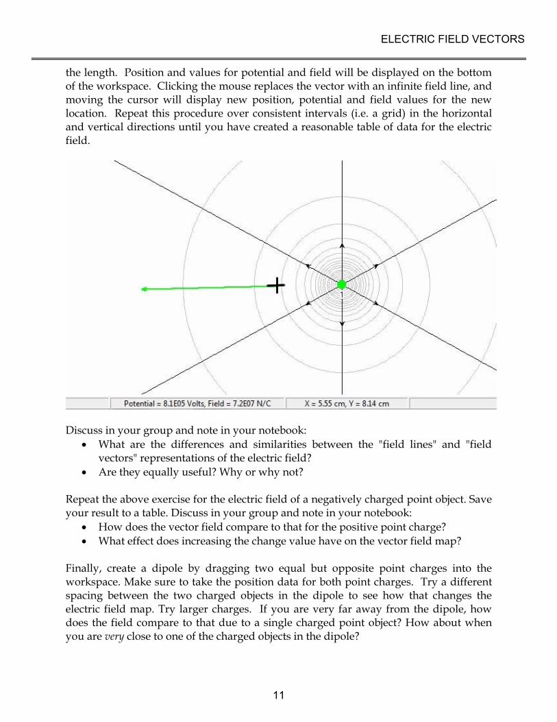
ELECTRIC FIELD VECTORS
the length. Position and values for potential and field will be displayed on the bottom of the workspace. Clicking the mouse replaces the vector with an infinite field line, and moving the cursor will display new position, potential and field values for the new location. Repeat this procedure over consistent intervals (i.e. a grid) in the horizontal and vertical directions until you have created a reasonable table of data for the electric field.
Discuss in your group and note in your notebook:
What are the differences and similarities between the "field lines" and "field vectors" representations of the electric field?
Are they equally useful? Why or why not? Repeat the above exercise for the electric field of a negatively charged point object. Save your result to a table. Discuss in your group and note in your notebook:
How does the vector field compare to that for the positive point charge?
What effect does increasing the change value have on the vector field map?
Finally, create a dipole by dragging two equal but opposite point charges into the workspace. Make sure to take the position data for both point charges. Try a different spacing between the two charged objects in the dipole to see how that changes the electric field map. Try larger charges. If you are very far away from the dipole, how does the field compare to that due to a single charged point object? How about when you are very close to one of the charged objects in the dipole?
11

ELECTRIC FIELD VECTORS
Make a table of the electric field caused by a dipole. It is especially important that you take your vector data moving equal increments in the horizontal and vertical directions. Save your results to a table. You should experiment with other electric field representations. Specifically, try to understand what role symmetry plays in the creation of electric fields.
ANALYSIS
Consider your dipole electric vector data.
Sketch the electric field as a function of position along the parallel axis of symmetry. Repeat for the perpendicular axis. How do these graphs compare with your prediction?
If you are very far away from the dipole, how does the field compare to that of a single point charge? How does it compare if you are very close to one of the point charges?
In general, where are the maxima and minima of the electric field? Does your answer depend on whether you are considering one or the other axes of symmetry? Why or why not?
Consider one of the electric field vectors in one of the diagrams you have created. If a positively charged object were placed at the tail end of that vector, what would be the direction of the force on it? What if it were a negatively charged object? How does the magnitude of the force compare to that of the force at a different point in space where the electric field vector is shorter or longer?
CONCLUSION
How does the computer-generated data compare with your corresponding predictions? What part of your prediction, if any, differed from the result? Why? Suppose you placed a positively charged point object near the dipole at three different locations. If the object began at rest, how would it move? What about if it started with some given initial velocity? Overall, was your prediction successful? Why or why not?
12

PROBLEM #2: ELECTRIC FIELD FROM A DIPOLE
You have a summer job with a solar power company. To measure the electric fields produced by solar cells, the company plans to use conductive paper. They will arrange the cells on the paper and measure the field at different points on the paper. You are assigned to test the soundness of this process for measuring the fields by using it to determine the electric field created by a simple pattern of charged objects. You create a two-dimensional dipole field by giving two parallel metal rods opposite charges with a battery while their tips are in contact with a sheet of conducting paper. You then measure the electric field in the paper. To see if the paper can be used to correctly map an electric field, you first make a detailed qualitative prediction of the electric field produced by an electric dipole at different points in space. Instructions: Before lab, read the required reading from the textbook and the laboratory in its entirety. In your lab notebook, respond to the warm up questions and derive a specific prediction for the outcome of the lab. During lab, compare your warm up responses and prediction in your group. Then, work through the exploration, measurement, analysis, and conclusion sections in sequence, keeping a record of your findings in your lab notebook. It is often useful to use Excel to perform data analysis, rather than doing it by hand. At the end of lab, disseminate any electronic copies of your results to each member of your group. Read: Mazur Sections 23.1 - 23.4 & 23.6.
EQUIPMENT
You have electrostatic paper, two brass rods (to serve as electrodes), banana cables, alligator clips, a battery and a wood block to increase contact pressure between the electrodes and the paper. Measurements will be made using a Digital Multimeter (DMM) set to read volts connected to a pin tip probe. You will also have the Electrostatics 3D program. A white sheet of paper with a grid similar to the grid on the conducting paper is useful for recording the field (do not write on the conductive
paper).
Overhead view of setup.
Read the sections Electrostatic Paper and Accessories and The Digital Multimeter (DMM) in the Equipment appendix.
If equipment is missing or broken, submit a problem report by sending an email to [email protected]. Include the room number and brief description of the problem.
13

ELECTRIC FIELD FROM A DIPOLE
WARM UP
1. Draw a picture of the dipole (one positive charge and one negative charge separated
by a distance d). Label the charged point objects “+” and “-”. Clearly define an x-y coordinate system.
2. Choose an arbitrary position on the dipole diagram. At this position, draw two
vectors, one each to represent the electric field due to each point charge. (Remember that you can understand the electric field at a particular location by considering the electric force on a positive “test charge” placed at that point.) How should the length and direction of each vector depend on the position relative to each charged object? What law governs this? Measure the distance from each charged object to the point where you are drawing the vectors to ensure the vectors have correct relative lengths.
3. Draw a darker vector representing the TOTAL electric field at that point. Remember
that a total, or net, electric field is constructed at a given position using the law of superposition (vectors add according to the tail-to-head vector sum rule).
4. Repeat this process at different, systematically chosen points (i.e., a grid) until you
have a reasonable map of the electric field in the space surrounding the dipole. Where is the field the strongest? The weakest? What is the direction of the field at different points along the dipole’s two different axes of symmetry? Sketch the electric field as function of position along the two axes of symmetry (two different graphs).
PREDICTION
Determine the physics task from the problem statement, and then in one or a few sentences, equations, drawings, and/or graphs, make a clear and concise prediction that solves the task. (Hint: How can you make a qualitative prediction with as much detail as possible?)
EXPLORATION
Systematically construct an electric field map using the Electrostatics 3D program. For instructions on how to use this program see the Exploration section of the “Electric Field Vectors” lab problem. Save your result to pdf. Next, construct a physical model of a dipole using the battery, rods, and conductive paper. Make sure to read the suggested appendix materials for details on how to use the
14

ELECTRIC FIELD FROM A DIPOLE
DMM and the conductive paper setup. Follow the instructions given there to set up the conductive paper. Once the rods are connected to the battery, set the digital multimeter (DMM) to DC volts and turn it on. Place the tips of the probe on the conductive paper midway between the tips of the two rods. Adjust the units on the DMM until you obtain reasonable readings. Recall the field maps you generated in the warm up questions and with the simulation software. Rotate the probe so that the center of the probe stays in the same spot. Do the values change (pay attention to the sign)? Is there a minimum or maximum value as you rotate the probe? Are there any apparent symmetries as you rotate the probe? If there are large fluctuations in the readings, determine how you will measure consistently. Determine how you will use the probe to determine the electric field direction at other points. Now place the field probe near, but not touching, one of the rods and rotate the probe as you did before. Record your data. Determine the direction of the electric field. Compare the maximum DMM reading at this point to the one you found at the midway point. Compare your measurements to your prediction; does the value displayed on the DMM become larger or smaller when the electric field becomes stronger? Consider how you will use the probe to determine the electric field strength at other points. Test a few more key points on the conductive paper. Where on the conductive paper is the electric field strongest? Weakest? Consider whether your observations match your predictions. Discuss in your group how you will use the probe to determine the field strength and direction at an arbitrary point on the conductive paper and how you will record the results on the white copy of the conductive paper. Discuss how you could construct a systematic map (hint: think grid) of the dipole’s electric field. IMPORTANT: Disseminate electronic copies of your results to each member of your group.
MEASUREMENT
Complete your measurement plan for mapping the electric field on the conductive paper. Select a point on the conductive paper where you wish to determine the electric field and determine its magnitude and direction at that point. Repeat the measurement to gain an estimate of the measurement uncertainty. Record the result on the white copy of the conductive paper. Repeat for as many points as needed to systematically create a field map that can be used to check your prediction.
15

ELECTRIC FIELD FROM A DIPOLE
ANALYSIS AND CONCLUSION
How does your map compare to your prediction? How does it compare to the simulation program? Where is the field strongest? How do you show this in your map? Where is the field weakest? How do you show this in your map? Do your answers somehow depend on the axis of symmetry under consideration? Overall, was your prediction successful? Why or why not?
16
PROBLEM #3: GRAVITATIONAL FORCE ON THE ELECTRON
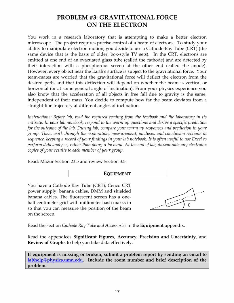
You work in a research laboratory that is attempting to make a better electron microscope. The project requires precise control of a beam of electrons. To study your ability to manipulate electron motion, you decide to use a Cathode Ray Tube (CRT) (the same device that is the basis of older, box-style TV sets). In the CRT, electrons are emitted at one end of an evacuated glass tube (called the cathode) and are detected by their interaction with a phosphorous screen at the other end (called the anode). However, every object near the Earth's surface is subject to the gravitational force. Your team-mates are worried that the gravitational force will deflect the electron from the desired path, and that this deflection will depend on whether the beam is vertical or horizontal (or at some general angle of inclination). From your physics experience you also know that the acceleration of all objects in free fall due to gravity is the same, independent of their mass. You decide to compute how far the beam deviates from a straight-line trajectory at different angles of inclination. Instructions: Before lab, read the required reading from the textbook and the laboratory in its entirety. In your lab notebook, respond to the warm up questions and derive a specific prediction for the outcome of the lab. During lab, compare your warm up responses and prediction in your group. Then, work through the exploration, measurement, analysis, and conclusion sections in sequence, keeping a record of your findings in your lab notebook. It is often useful to use Excel to perform data analysis, rather than doing it by hand. At the end of lab, disseminate any electronic copies of your results to each member of your group. Read: Mazur Section 23.5 and review Section 3.5.
EQUIPMENT
You have a Cathode Ray Tube (CRT), Cenco CRT power supply, banana cables, DMM and shielded banana cables. The fluorescent screen has a one-half centimeter grid with millimeter hash marks in so that you can measure the position of the beam on the screen.
Read the section Cathode Ray Tube and Accessories in the Equipment appendix. Read the appendices Significant Figures, Accuracy, Precision and Uncertainty, and Review of Graphs to help you take data effectively.
If equipment is missing or broken, submit a problem report by sending an email to [email protected]. Include the room number and brief description of the problem.
17
GRAVITATIONAL FORCE ON THE ELECTRON
WARM UP
1. Draw a picture of the CRT in the horizontal position. Do not include the deflection
plates shown in the appendix diagrams since they will not be used in this lab. Draw the electron's trajectory from the time it leaves the electron gun until it hits the screen. Label each important kinematics quantity in the problem. Using a free body diagram, label all forces on the electron during this time. Choose a convenient coordinate system and put it on your drawing. Does the vertical component of the electron's velocity change? Why or why not? Does the horizontal component of its velocity change? Why or why not?
2. Calculate the velocity of the electron just after it leaves the electron gun.
Hint: The change in the electric potential energy of an electron moving across a pair of acceleration plates is the voltage difference between the two plates times the electron's charge. What basic physics principle can you use to calculate the electron’s velocity as it exits the electron gun? What assumptions must you make to carry out this calculation?
3. What physics principle(s) can you use to calculate how far the electron falls below a
straight-line trajectory due to the force of gravity? What quantities must you know to make the calculation? Perform this calculation to find a symbolic and then a numerical answer.
4. Does your solution make sense? You can check by estimating the time of flight of the
electron based on its initial velocity and the distance between its starting point and the screen. In that amount of time, how far would a ball drop in free fall? If the solution does not make sense, check your work for logic or algebra mistakes.
5. Repeat 1-4 for a CRT pointed directly upwards, finding first a symbolic and then a
numerical answer. 6. Finally, repeat 1-4 at an arbitrary inclination angle from the horizontal. State your
answer symbolically and then numerically (a number times a function of the inclination angle, in this case).
IMPORTANT hints: (1) Try using a reference frame where x is always along and y is always perpendicular to the electron’s initial trajectory. (2) If your equations become complicated, make useful approximations by considering how large any term that contains the electron’s velocity is relative to other terms in a given equation. (3) Does your arbitrary angle answer agree with the strictly horizontal and strictly vertical cases?
18

GRAVITATIONAL FORCE ON THE ELECTRON
PREDICTION
Determine the physics task from the problem statement, and then in one or a few sentences, equations, drawings, and/or graphs, make a clear and concise prediction that solves the task. (Hint: How can you make a qualitative prediction with as much detail as possible?)
EXPLORATION
WARNING: You will be working with equipment that generates large electric voltages. Improper use can cause painful burns. The power must be turned off and you must wait at least one minute before any wires are disconnected from or connected to the power supply. Never touch the conducting metal of any wire.
Follow the directions in the appendix for connecting the power supply to the CRT. Check to see that the connections from the power supply to the high voltage and the filament heater are correct, before you turn the power supply on. You should have a difference of ~250-500 Volts of electric potential between the cathode and anode. After a moment, you should see a spot that you can adjust with the knob labeled “Focus”. Note the details of all the connections in your lab notebook. (If your connections are correct and the spot still does not appear, inform your lab instructor.) Discuss the following in your group and note your responses in your lab notebook.
Do you expect the gravitational deflection to vary as a function of the angle of the CRT with the horizontal? Try different orientations in the horizontal plane to see if you can observe any difference. Does the observed behavior of the electron deflection agree with your prediction?
For what orientation of the CRT is it impossible for the gravitational force to deflect the electron? This is the location of the beam spot when there is no gravitational effect on the motion of the electrons and should be used as the origin (and NOT the arbitrary origin on grid).
Do you observe any deflection of the electron beam? How can you determine if this deflection is or is not caused by the gravitational force? If it is not, how can you minimize such effects on your measurements?
Devise a measurement scheme to record the angle of the CRT and the position of the beam spot and record you measurement plan. (In general, a measurement plan minimally consists of three labeled columns of numbers with units: (1) the independent variable that you vary (you should pre-determine at which values of the independent variable you will perform your measurements; also, what is the independent variable in this experiment?), (2) the predicted values of the dependent variable (i.e., use your prediction equation to compute what measurement you expect
19

GRAVITATIONAL FORCE ON THE ELECTRON
to observe at each value of the independent variable; what is the dependent variable for this experiment), and (3) the actual, measured values of the independent variable. Try doing this in Excel, as the computational power of using a computer program will make doing labs easier as the labs themselves become more difficult.)
MEASUREMENT
Following your measurement scheme, measure the position of the beam spot at an orientation of the CRT for which you expect the gravitational deflection to be zero and then at the orientation for which you expect the gravitational deflection to be maximum. Finally, make measurements at several different intermediate angles of inclination. Note: Be sure to record your measurements with the appropriate number of significant figures and with your estimated uncertainty Otherwise, the data is virtually meaningless. If necessary, read the suggested appendix material.
ANALYSIS
Use your data to determine the magnitude of the deflection of the electron. Make a graph of the position of the electron beam spot as a function of the angle that the CRT makes with the horizontal for both your predicted and measured deflection values. If you observe a deflection, how can you tell if it is caused by the gravitational force? If the deflection is not caused by gravity, what might be its cause? How will you decide?
CONCLUSION
Did you observe any deflection of the electron beam? Was it in the direction you expected due to the gravitational force? Did you observe any aberrant behavior? What could account for this? How did you conduct the experiment to minimize any aberrant behavior? Can you measure the effect of the Earth's gravitational force on the motion of the electrons in the CRT? Why or why not? Based on your results, do you think you need to take gravitational deflection into account when using the CRT? Why or why not? Overall, was your prediction successful? Why or why not?
20

PROBLEM #4: DEFLECTION OF AN ELECTRON BEAM BY AN ELECTRIC FIELD
You are attempting to design an electron microscope. To precisely steer the beam of electrons you will use an electric field perpendicular to the original direction of the electrons. To test the design, you must determine how a change in the electric field strength affects the position of the beam spot. A colleague argues that an electron’s trajectory through an electric field is analogous to a bullet’s trajectory through a gravitational field. You are not convinced but are willing to test the idea. One difference that you both agree on is that the electrons in the microscope will pass through a region with an electric field and other regions with no electric field, while a bullet is always in a gravitational field. You decide to model the situation with a Cathode Ray Tube (CRT) in which electrons are emitted at one end of an evacuated glass tube and are detected by their interaction with a phosphorous screen on the other end. You will calculate the deflection of an electron that begins with an initial horizontal velocity, passes between a pair of short metal plates that produce a vertical electric field between them, and then continues through a region with no electric field until hitting the screen. Your result could depend on the strength of the electric field, the electron’s initial velocity, intrinsic properties of the electron, the length of the metal plates that produce the vertical electric field, and the distance from the end of the metal plates to the screen. Your goal is to determine deflection as a function of electric field strength. Instructions: Before lab, read the required reading from the textbook and the laboratory in its entirety. In your lab notebook, respond to the warm up questions and derive a specific prediction for the outcome of the lab. During lab, compare your warm up responses and prediction in your group. Then, work through the exploration, measurement, analysis, and conclusion sections in sequence, keeping a record of your findings in your lab notebook. It is often useful to use Excel to perform data analysis, rather than doing it by hand. At the end of lab, disseminate any electronic copies of your results to each member of your group. Read: Mazur Section 23.5 and review Section 3.5.
EQUIPMENT
You have a Cathode Ray Tube. You also have a Cenco power supply, banana cables, DMM and an 18v/5amp power supply. The applied electric field is created by connecting the internal parallel plates to the power supply. Note: The CENCO power supplies can have transient AC voltage in the DC output, making it less than ideal for creating an electric field – use the 18volt/5amp supplies.
Read the section Cathode Ray Tube and Accessories in the Equipment appendix. Read the appendices Significant Figures, Accuracy, Precision and Uncertainty, and Review of Graphs to help you take data effectively.
21

DEFLECTION OF AN ELECTRON BEAM BY AN ELECTRIC FIELD
If equipment is missing or broken, submit a problem report by sending an email to [email protected]. Include the room number and brief description of the problem.
WARM UP
1. Examine the diagram of the CRT in the appendix. You will use only one set of the
deflection plates shown. Draw a simplified diagram of an electron with an initial horizontal velocity about to enter the region between the plates. Draw the screen some distance past the end of the plates. Label the relevant distances. Assume that the electric field is vertically oriented in the region between the plates and is zero elsewhere. Indicate on your picture where an electron experiences electrical forces. Draw a coordinate axis on this picture. Sketch the electron's trajectory through the CRT, indicating where the electron should accelerate and the direction of that acceleration. Indicate on the screen of the CRT the distance by which the electron has been deflected away from its initial straight-line path. Why can you ignore the gravitational force on the electron?
2. Recall some things you already know about projectile motion. Does a force in the
vertical direction affect the horizontal component of an object’s velocity? In this situation, can you use the horizontal velocity component to find the time required to travel some horizontal distance?
3. Consider the motion of the electron in the region between the deflection plates.
Calculate the amount of time the electron spends in this region. Calculate the vertical position and vertical velocity component of the electron when it leaves this region. Remember you are assuming that only an electric force acts on the electron and are neglecting the gravitational force. (You will need the relationship between the electric field and the electric force on a charged object, as well as the general relationship between force and acceleration.)
4. Consider the motion of the electron in the region past the deflection plates. What is
true about the vertical and horizontal components of its velocity in this region? Calculate where the electron hits the screen relative to where it entered this final region. Then calculate the total deflection of the electron at the screen from where it initially entered the region between the plates.
5. Using the equation you have found for the deflection of the electron beam, draw a
graph of the deflection vs. the electric field. Treat the other quantities as constant. 6. Two quantities in your expression are not directly measurable in lab. These are the
electron’s initial velocity and the electric field strength between the deflection plates. You will, however, know the voltage that accelerates the electrons, Vacc, and the voltage across the deflection plates, Vplates . Use conservation of energy to express the
22
DEFLECTION OF AN ELECTRON BEAM BY AN ELECTRIC FIELD
electron’s initial velocity in terms of Vacc. Substitute this expression into your deflection equation.
Hint: The change in the electric potential energy of an electron moving from one plate to another is the voltage difference between the two plates (Vacc in the appendix diagram) times the electron's charge. What assumptions must you make to calculate the electron’s initial velocity?
7. Write an equation relating Vplates to the electric field between the plates, and
substitute it into your deflection equation. Your final deflection equation should involve only quantities that can be measured in lab or found in the textbook or appendix.
Hint: the electric field between the plates equals Vplates divided by the distance between the plates.
PREDICTION
Determine the physics task from the problem statement, and then in one or a few sentences, equations, drawings, and/or graphs, make a clear and concise prediction that solves the task. (Hint: How can you make a qualitative prediction with as much detail as possible?)
EXPLORATION
WARNING: You will be working with equipment that generates large electric voltages. Improper use can cause painful burns. To avoid danger, the power must be turned off and you must wait at least one minute before any wires are disconnected from or connected to the power supply. Never touch the conducting metal of any wire.
Follow the directions in the appendix for connecting the power supply to the CRT. Check to see that the connections from the power supply to the high voltage and the filament heater are correct, before you turn the power supply on. Apply between 250 and 500 Volts across the anode and cathode. After a moment, you should observe a spot on the screen that can be adjusted with the knob labeled “Focus”. If your connections are correct and the spot still doesn’t appear, inform your lab instructor. TAKING EXTREME CARE!, change the voltage across the accelerating plates, and determine the range of values for which the electrons have enough energy to produce a spot on the screen. Changing this voltage changes the velocity of the electrons as they enter the deflection plates. What is the range of initial electron velocities corresponding to this range of accelerating voltages? Which of these values will give you the largest deflection when you later apply an electric field between the deflection plates?
23

DEFLECTION OF AN ELECTRON BEAM BY AN ELECTRIC FIELD
Before you turn on the electric field between the deflection plates, make a note of the position of the spot on the screen. The deflections you measure will be in relation to this point. Make sure not to change the position of the CRT since external fields may affect the position of the spot. Now apply a voltage across one set of deflection plates, noting how the electron beam moves across the screen as the voltage is increased. Find a voltage across the acceleration plates that allows the deflection for the entire range of deflection plate voltages to be measured as accurately as possible. Devise a measuring scheme to record the position of the beam spot. Be sure you have established the zero deflection point of the beam spot. Write down your measurement plan. How will you determine the strength of the electric field between the deflection plates? How will you determine the initial velocity of the electrons? What quantities will you hold constant for this measurement? How many measurements do you need?
MEASUREMENT
Measure the position of the beam spot as you vary the electric field applied to the deflection plates, keeping other parameters constant. At least two people should make a measurement at each point, so you can estimate measurement uncertainty. Note: Be sure to record your measurements with the appropriate number of significant figures and with your estimated. Otherwise, the data is virtually meaningless. If necessary, refer to the suggested appendix material.
ANALYSIS
Graph the measured deflection of the electron beam as a function of the voltage difference across the deflector plates. Display uncertainties on your graph.
CONCLUSION
Did your data agree with your prediction of how the electron beam deflection would depend on the electric field between the deflection plates? If not, why? How does the deflection of the electron beam vary with the electric field? State your results in the most general terms supported by your data.
24

PROBLEM #5: DEFLECTION OF AN ELECTRON BEAM AND VELOCITY
You are attempting to design an electron microscope. To precisely steer the beam of electrons you will use an electric field perpendicular to the original direction of the electrons. To test the design, you must determine how a change in the initial velocity of the electrons affects the position of the beam spot. A colleague argues that an electron’s trajectory through an electric field is analogous to a bullet’s trajectory through a gravitational field. You are not convinced but are willing to test the idea. One difference that you both agree on is that the electrons in the microscope will pass through a region with an electric field and other regions with no electric field, while a bullet is always in a gravitational field. You decide to model the situation with a Cathode Ray Tube (CRT) in which electrons are emitted at one end of an evacuated glass tube and are detected by their interaction with a phosphorous screen on the other end. You will calculate the deflection of an electron that begins with an initial horizontal velocity, passes between a pair of short metal plates that produce a vertical electric field between them, and then continues through a region with no electric field until hitting the screen. Your result could depend on the strength of the electric field, the electron’s initial velocity, intrinsic properties of the electron, the length of the metal plates that produce the vertical electric field, and the distance from the end of the metal plates to the screen. Your goal is to determine deflection as a function of the initial electron speed. Read: Mazur Section 23.5 and review Section 3.5.
EQUIPMENT
You have a Cathode Ray Tube. You also have a Cenco power supply, banana cables, DMM and an 18v/5amp power supply. The applied electric field is created by connecting the internal parallel plates to the power supply. Note: The CENCO power supplies can have transient AC voltage in the DC output, making it less than ideal for creating an electric field – use the 18volt/5amp supplies.
Read the section Cathode Ray Tube and Accessories in the Equipment appendix. Read the appendices Significant Figures, Accuracy, Precision and Uncertainty, and Review of Graphs to help you take data effectively.
If equipment is missing or broken, submit a problem report by sending an email to [email protected]. Include the room number and brief description of the problem.
25

DEFLECTION OF AN ELECTRON BEAM AND VELOCITY
WARM UP
1. Examine the diagram of the CRT in the appendix. You will use only one set of the
deflection plates shown. Draw a simplified diagram of an electron with an initial horizontal velocity about to enter the region between the plates. Draw the screen some distance past the end of the plates. Label the relevant distances. Assume that the electric field is vertically oriented in the region between the plates and is zero elsewhere. Indicate on your picture where an electron experiences electrical forces. Draw a coordinate axis on this picture. Sketch the electron's trajectory through the CRT, indicating where the electron should accelerate and the direction of that acceleration. Indicate on the screen of the CRT the distance by which the electron has been deflected away from its initial straight-line path. Why can you ignore the gravitational force on the electron?
2. Recall some things you already know about projectile motion. Does a force in the
vertical direction affect the horizontal component of an object’s velocity? In this situation, can you use the horizontal velocity component to find the time required to travel some horizontal distance?
3. Consider the motion of the electron in the region between the deflection plates.
Calculate the amount of time the electron spends in this region. Calculate the vertical position and vertical velocity component of the electron when it leaves this region. Remember you are assuming that only an electric force acts on the electron and are neglecting the gravitational force. (You will need the relationship between the electric field and the electric force on a charged object, as well as the general relationship between force and acceleration.)
4. Consider the motion of the electron in the region past the deflection plates. What is
true about the vertical and horizontal components of its velocity in this region? Calculate where the electron hits the screen relative to where it entered this final region. Then calculate the total deflection of the electron at the screen from where it initially entered the region between the plates.
5. Using the equation you have found for the deflection of the electron beam draw a
graph of the deflection vs. the initial velocity. Treat the other quantities as constant. 6. Two quantities in your expression are not directly measurable in lab. These are the
electron’s initial velocity and the electric field strength between the deflection plates. You will, however, know the voltage that accelerates the electrons, Vacc , and the voltage across the deflection plates, Vplates . Use conservation of energy to express the electron’s initial velocity in terms of Vacc . Substitute this expression into your deflection equation.
26
DEFLECTION OF AN ELECTRON BEAM AND VELOCITY
Hint: The change in the electric potential energy of an electron moving from one plate to another is the voltage difference between the two plates times the electron's charge. What assumptions must you make to calculate the electron’s initial velocity?
7. Write an equation relating Vplates to the electric field between the plates, and
substitute it into your deflection equation. Your final deflection equation should involve only quantities that can be measured in lab or found in the textbook or appendix.
Hint: the electric field between the plates equals Vplates divided by the distance between the plates.
PREDICTION
Determine the physics task from the problem statement, and then in one or a few sentences, equations, drawings, and/or graphs, make a clear and concise prediction that solves the task. (Hint: How can you make a qualitative prediction with as much detail as possible?)
EXPLORATION
WARNING: You will be working with equipment that generates large electric voltages. Improper use can cause painful burns. To avoid danger, the power must be turned off and you must wait at least one minute before any wires are disconnected from or connected to the power supply. Never touch the conducting metal of any wire.
Follow the directions in the appendix for connecting the power supply to the CRT. Check to see that the connections from the power supply to the high voltage and the filament heater are correct before you turn the power supply on. Apply between 250 and 500 Volts across the anode and cathode. After a moment, you should observe a spot on the screen that can be adjusted with the knob labeled “Focus”. If your connections are correct and the spot still doesn’t appear, inform your lab instructor. TAKING EXTREME CARE!, change the voltage across the accelerating plates, and determine the range of values for which the electrons have enough energy to produce a spot on the screen. Changing this voltage changes the velocity of the electrons as they enter the deflection plates. What is the range of initial electron velocities corresponding to this range of accelerating voltages? Which of these values will give you the largest deflection when you later apply an electric field between the deflection plates?
27

DEFLECTION OF AN ELECTRON BEAM AND VELOCITY
Before you turn on the electric field between the deflection plates, make a note of the position of the spot on the screen. The deflections you measure will be in relation to this point. Make sure not to change the position of the CRT since external fields may affect the position of the spot. Now apply a voltage across one set of deflection plates, noting how the electron beam moves across the screen as the initial electron velocity is increased. Find a voltage across the deflection plates that allows the deflection for the entire range of initial electron velocities to be measured as accurately as possible. Devise a measuring scheme to record the position of the beam spot. Be sure you have established the zero deflection point of the beam spot. Write down your measurement plan. How will you determine the strength of the electric field between the deflection plates? How will you determine the initial velocity of the electrons? What quantities will you hold constant for this measurement? How many measurements do you need?
MEASUREMENT
Measure the deflection of the beam spot as you vary the initial velocity of the electrons in the beam, keeping other parameters constant. At least two people should make a measurement at each point, so you can estimate measurement uncertainty. Note: Be sure to record your measurements with the appropriate number of significant figures and with your estimated uncertainty. Otherwise, the data is virtually meaningless. If necessary, refer to the suggested appendix material to help determine these.
ANALYSIS
Graph the measured deflection of the electron beam as a function of initial electron speed. Display uncertainties on your graph.
CONCLUSION
Did your data agree with your prediction of how the electron beam deflection would depend on the initial electron velocity? If not, why? How does the deflection of the electron beam vary with initial electron velocity? State your results in the most general terms supported by your data.
28
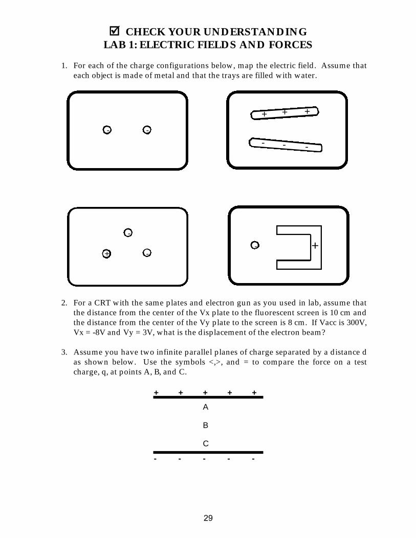
CHECK YOUR UNDERSTAN DING
LAB 1: ELECTRIC FIELDS AND FORCES
1. For each of the charge configurations below, map the electric field . Assume that
each object is made of metal and that the trays are filled with water.
2. For a CRT with the same plates and electron gun as you used in lab, assume that
the d istance from the center of the Vx plate to the fluorescent screen is 10 cm and
the d istance from the center of the Vy plate to the screen is 8 cm. If Vacc is 300V,
Vx = -8V and Vy = 3V, what is the d isplacement of the electron beam?
3. Assume you have two infinite parallel planes of charge separated by a d istance d
as shown below. Use the symbols <,>, and = to compare the force on a test
charge, q, at points A, B, and C.
C
B
A
+ ++ ++
- ----
-
+
-
-
-
++ +
-- -
- +
29

CHECK YOUR UNDERSTAN DING
LAB 1: ELECTRIC FIELDS AND FORCES
30

Physics Lab Report Rubric
Name: ID#:Course, Lab Sequence, and Problem Number:Date Performed:Lab Partners’ Names:
Possible Earned
Warm-Up Questions
Possible Earned
Laboratory Notebook
Earns No Points Earns Full Points Possible EarnedArgument
• no clear argument• logic does not flow• gaps in content• leaves reader with questions
• complete, cogent, flowing argument• context, execution, analysis, conclu-
sion all present• leaves reader satisfied
Technical Style
• vocabulary, syntax, etc. inappropri-ate for scientific writing
• necessary nonverbal media absent orpoorly constructed
• subjective, fanciful, or appealing toemotions
• jarringly inconsistent
• language is appropriate• nonverbal media present where ap-
propriate, well constructed, well in-corporated
• objective, indicative, logical style• consistent style• division into sections is helpful
Use of Physics
• predictions with no or with unphysi-cal justification
• experiment physically unjustified• experiment tests wrong phenomenon• theory absent from consideration of
premise, predictions, and results
• predictions are justified with physicaltheory
• experiment is physically sound andactually tests phenomenon in ques-tion
• results interpreted with theory toclear, appropriate conclusion
Quantitativeness
• statements are vague or arbitrary• analysis is inappropriately qualitative• error analysis not used to evaluate
prediction or find result• numbers, equations, units, uncertain-
ties missing or inappropriate
• consistently quantitative• equations, numbers with units, uncer-
tainties throughout• prediction confirmed or denied, result
found by error analysis• results, conclusions based on data
Total
31

32
LAB 2: ELECTRIC FIELDS AND ELECTRIC POTENTIALS
In this lab you will continue to investigate the abstract concept of electric field . If you
know the electric field at a point in space, you can easily determine the force exerted
on a charged object placed at that point. The concept of field has the practical
advantage that you can determine the forces on an object in two stages. To determine
the force exerted on object A by other objects, you first determine the field , at a
location to be occupied by A, due to all objects except for object A . You then calculate the
force exerted on object A by that field . That force depends only on the properties of
object A and the value of the field at object A’s location. An advantage of this two-step
approach is that if you make no changes but replace object A with a new object, B, it is
simple to calculate the force exerted on object B. This is because replacing A with B
does not change the field . The field that exerts a force on an object depends only on the other
objects.
Keeping track of forces and accelerations is not always the simplest approach for
predicting the behavior of objects. It is often more convenient to use the principle of
Conservation of Energy. As mentioned in the introduction to the previous lab, the
potential energy related to the position of a charged object resides in the surrounding
field . As with forces on an object (A) due to a field , the change in potential energy
due to the addition of an object (A) to a configuration of other objects is calculated in
two stages. First you calculate the “potential,” at a location to be occupied by object A,
due to all objects except for object A . That potential depends only on the other objects
and does not depend on any properties of object A. You then use the value of the
potential at that location to calculate the change in potential energy when object A is
placed there. That potential energy depends only on the properties of object A and the
value of the potential at object A’s location. As with forces, it would then be a simple
matter to calcu late the potential energy change due to replacing object A with another
object B.
Because the concepts of field and potential are abstract and d ifficult to visualize, this
laboratory uses a computer simulation based on the interaction of point charged objects
(usually called point charges). With this simulation you can construct a complicated
charge configuration and read out the resulting electric field and electric potential at
any point in space.
OBJECTIVES
After successfully completing this laboratory, you should be able to:
Qualitatively determine the electric field at a point in space caused by a
configuration of charged objects based on the geometry of those objects.
Calculate the electric field at a point in space caused by a configuration of cha rged
objects based on the geometry of those objects.
33

LAB 2: ELECTRIC FIELDS AND ELECTRIC POTENTIALS
Qualitatively determine the electric potential at a point in space caused by a
configuration of charged objects based on the geometry of those objects.
Calculate the electric potential at a point in space caused by a configuration of
charged objects based on the geometry of those objects.
Relate the electric field caused by charged objects to the electric potential caused by
charged objects.
PREPARATION
Read: Mazur Chapters 23 and 25
Before coming to lab you should be able to:
Add vectors in two d imensions.
Calculate the electric field due to a point charge.
Calculate the electric potential due to a point charge.
Use the computer simulation program, Electrostatics 3D.
34

PROBLEM #1: THE ELECTRIC FIELD FROM MULTIPLE POINT CHARGES
You work with a biochemical engineering group investigating new insulin-fabrication techniques. Part of your task is to calculate electric fields produced by complex molecules. The team has decided to use a computer simulation to calculate the fields. Your task is to determine if the simulation agrees with the physics that you know. You decide to determine the electric field at a point from a set of charged objects that is complex enough to test the simulation but simple enough to make direct calculation possible. The first configuration you try is a square with two equal negatively charged point objects in opposite corners and a positively charged point object of 1/3 the magnitude of the negative charges in a third corner. You will calculate the electric field at the remaining corner of the square and compare your result to that from the computer simulation of the same configuration. Instructions: Before lab, read the required reading from the textbook and the laboratory in its entirety. In your lab notebook, respond to the warm up questions and derive a specific prediction for the outcome of the lab. During lab, compare your warm up responses and prediction in your group. Then, work through the exploration, measurement, analysis, and conclusion sections in sequence, keeping a record of your findings in your lab notebook. It is often useful to use Excel to perform data analysis, rather than doing it by hand. At the end of lab, disseminate any electronic copies of your results to each member of your group. Read: Mazur Chapter 23. Read carefully Sections 23.3 & 23.5.
EQUIPMENT
The computer program Electrostatics 3D, a protractor and a ruler.
If equipment is missing or broken, submit a problem report by sending an email to [email protected]. Include the room number and brief description of the problem.
WARM UP
1. Make a picture of the situation, carefully labeling the objects and their charges and all
distances and angles. At the point of interest (the point where you are calculating the electric field), draw and label the electric field vectors produced by the charged objects. Finally, place a useful coordinate system on your drawing.
2. Determine the magnitude and direction of each of these vectors. (You may need
geometry and trigonometry to determine distances and directions.) 3. Calculate the components of each vector with respect to your coordinate system.
35

THE ELECTRIC FIELD FROM MULTIPLE POINT CHARGES
4. Find the components of the total (net) electric field vector at the point of interest, and
then use them to write an expression for both the magnitude and direction of the total electric field vector at the point of interest. (Recall what you read about addition of vectors in the textbook.)
PREDICTION
Determine the physics task from the problem statement, and then in one or a few sentences, equations, drawings, and/or graphs, make a clear and concise prediction that solves the task.
EXPLORATION
In the folder Physics on the desktop, open Electrostatics 3D and click on the Point Charge button found on the far left side of the toolbar. You can now place a point charge within the workspace. Once placed, a dialog box opens allowing you to enter the magnitude of the point charge, and whether it is positive or negative.
Click the Electric Field line button and move the cursor within the workspace to where you would like to evaluate a field vector. An electric field vector will appear with direction given by the arrowhead and the relative magnitude given by the length.
36

THE ELECTRIC FIELD FROM MULTIPLE POINT CHARGES
Position and values for potential and field will be displayed on the bottom of the workspace. Clicking the mouse will cause the vector to be replaced by an infinite field line, and moving the cursor will display new position, potential and field values for the new location. You can reveal simulated electric field values anywhere in the workspace by moving the cursor where you would like to evaluate the electric field. To place objects at precise points on the screen you will need to keep track of the position data displayed at the bottom of the workspace. You might find it helpful to map out the (x) and (y) positions required in the workspace to simulate the assigned configurations. To check whether or not you get the correct behavior of the electric field from a point charge do the following: 1. Pick a useful charge value and determine several locations at different distances r
from the center of the single point charge. (Hint: Choose your locations at regular intervals.) At each location, record the position and the electric field value. In your notebook, record the data and sketch a plot of the field strength as a function of r.
2. Now, calculate what Coulomb’s law predicts and sketch the values for the field
strength vs. distance (r) on the same graph. 3. Compare the shape of the graph to that based on Coulomb’s law and record your
observations. Now, explore the distribution of three charges. Drag two equal negative charges and one positive charge of 1/3 the value of one negative charge onto the screen in the configuration specified in the problem statement above. Make sure the charges are accurately placed using the position data. Note the length of the electric field vector in the fourth corner of the square. What parameter can you easily vary to change the length of the electric field vector in that corner while preserving the other conditions of the problem? In your notebook, note whether or not such manipulations change the direction of the electric field at that corner, and record the direction. Hint: you may need to change the box size or charge magnitudes to get vectors that are large enough to measure accurately but not so large that they go off the screen. Determine a measurement plan.
MEASUREMENT
Measure the field strength and record the direction of the electric field vector at the point of interest for several different values of the varying parameter, according to your measurement plan. Record the data in your notebook.
37
THE ELECTRIC FIELD FROM MULTIPLE POINT CHARGES
ANALYSIS
Use the data for the following analysis (perform in Excel):
1. Using your prediction equation, which is based on Coulomb’s law, calculate the expected electric field magnitudes in SI units at the point of interest for your chosen values of the variable parameter.
2. Compare your calculated electric field strength to that from the computer simulation on a plot. Also, compare your prediction of the direction of the field to that from the computer simulation.
CONCLUSION
How did your expected result compare to your measured result? Explain any differences. From your results, which general properties of the electric field does the simulation faithfully reproduce? What is the specific evidence?
38

PROBLEM #2: THE ELECTRIC FIELD FROM A LINE OF CHARGE
You are a member of a team designing an electrostatic air cleaner for the use of people suffering from allergies. The air passage through the device will contain many complicated charged electrodes. You must determine the effect of these electrodes on plant spores that cause allergic reactions. The first step is to calculate the electric field at every point in the air passage. Because the electrode configuration is complicated, your team has decided to use a computer simulation to model the resulting electric field. Your task is to determine if the simulation results agree with the physics you know for non-point-like charged objects. You decide to test the simulation for the case of a uniformly charged rod, since this situation is simple enough for you to calculate. For comparison with the simulation results, you decide to calculate the electric field at arbitrary points from the middle of the rod along its perpendicular axis and also at arbitrary points from the end of the rod along its parallel axis. Instructions: Before lab, read the required reading from the textbook and the laboratory in its entirety. In your lab notebook, respond to the warm up questions and derive a specific prediction for the outcome of the lab. During lab, compare your warm up responses and prediction in your group. Then, work through the exploration, measurement, analysis, and conclusion sections in sequence, keeping a record of your findings in your lab notebook. It is often useful to use Excel to perform data analysis, rather than doing it by hand. At the end of lab, disseminate any electronic copies of your results to each member of your group. Read: Mazur Section 23.7.
EQUIPMENT
The computer program Electrostatics 3D, a protractor and a ruler.
If equipment is missing or broken, submit a problem report by sending an email to [email protected]. Include the room number and brief description of the problem.
WARM UP
1. Make a picture of the situation. Select an arbitrary point of interest along the perpendicular axis for calculating the electric field. Label all relevant constant quantities, distances, and angles. Decide on an appropriate coordinate system. Draw a representative infinitesimal charge element dq somewhere along the rod.
2. Draw an infinitesimal electric field vector dE produced by dq at a single point of interest along the perpendicular axis of symmetry. Write an expression for its magnitude. Draw and label its components. Write expressions for each component.
39

THE ELECTRIC FIELD FROM A LINE OF CHARGE
3. Write an integral for each component of the total field at the point of interest in terms of dq. The total electric field due to a charge distribution is found by calculating the contribution from each charge element to the total (vector) field, and summing the contributions (as vectors). When the charge distribution is continuous, it can be mathematically divided into infinitesimal elements dq; then (for each field component) the individual contributions are added together with an integral. (Note: Always consider the symmetry of the situation. It may be that the integral for one of the components vanishes for some reason. Explore this.)
4 Evaluate the integral(s) you set up in question 3 to get an expression(s) for the electric field’s components at the point of interest. Write an expression for the total field magnitude and indicate its direction. In order to evaluate such an integral, all terms in the integrand must be either constants or explicit functions of the integration variable. First, choose an appropriate integration variable. Then, rewrite all variable quantities in the integrand (including dq) in terms of the integration variable you have chosen. Determine appropriate limits for the integration variable you have chosen. Use the Pythagorean Theorem, trigonometry, and the linear charge density to write your integrand(s) in a suitable form.
5. Repeat steps 1-4 for an arbitrary point of interest along the parallel axis.
PREDICTION
Determine the physics task from the problem statement, and then in one or a few sentences, equations, drawings, and/or graphs, make a clear and concise prediction that solves the task.
EXPLORATION
In the folder Physics on the desktop, open Electrostatics 3D and click on the Point Charge button found on the far left side of the toolbar. You can now place a point charge within the workspace. Once placed, a dialog box opens allowing you to enter the magnitude of the point charge, and whether it is positive or negative.
40
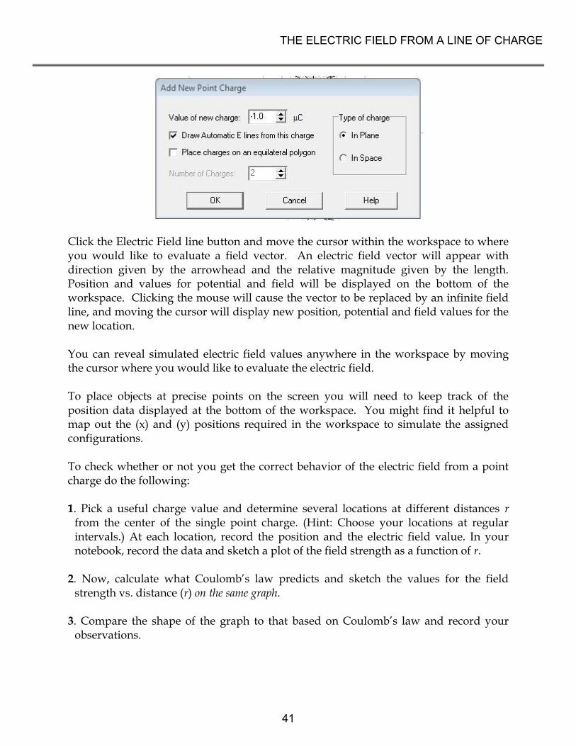
THE ELECTRIC FIELD FROM A LINE OF CHARGE
Click the Electric Field line button and move the cursor within the workspace to where you would like to evaluate a field vector. An electric field vector will appear with direction given by the arrowhead and the relative magnitude given by the length. Position and values for potential and field will be displayed on the bottom of the workspace. Clicking the mouse will cause the vector to be replaced by an infinite field line, and moving the cursor will display new position, potential and field values for the new location. You can reveal simulated electric field values anywhere in the workspace by moving the cursor where you would like to evaluate the electric field. To place objects at precise points on the screen you will need to keep track of the position data displayed at the bottom of the workspace. You might find it helpful to map out the (x) and (y) positions required in the workspace to simulate the assigned configurations. To check whether or not you get the correct behavior of the electric field from a point charge do the following: 1. Pick a useful charge value and determine several locations at different distances r
from the center of the single point charge. (Hint: Choose your locations at regular intervals.) At each location, record the position and the electric field value. In your notebook, record the data and sketch a plot of the field strength as a function of r.
2. Now, calculate what Coulomb’s law predicts and sketch the values for the field
strength vs. distance (r) on the same graph. 3. Compare the shape of the graph to that based on Coulomb’s law and record your
observations.
41

THE ELECTRIC FIELD FROM A LINE OF CHARGE
Now, explore the line charge configuration. From the toolbar or Add menu select Point Charge and create a line of charge by dragging individual positive charges onto the screen to create a long, uniform line of charge. Hints: make sure the charges are evenly distributed. Optimize the overall charge density and placement of the line on the screen in order to be able to obtain good measurements of electric field vectors. Display electric field vectors at the locations of interest for this problem, and investigate how the magnitude and direction of the electric field depends on position. Determine a measurement plan. After you’ve created a line of charge using individual point charges, create a line of charge using the continuous horizontal linear charge option of Electrostatics 3D. From the toolbar or Add menu select Horizontal Linear Charge. Select a charge density that is similar to the charge density of the line of charge you just created from individual point charges. Display electric field vectors at the locations of interest for this problem, and investigate how the magnitude and direction of the electric field depends on position. Determine a measurement plan.
MEASUREMENT
Measure the magnitude and direction of the electric field vector at varying locations along each axis of symmetry. Record the data in your notebook.
ANALYSIS
Use the data for the following analysis (perform in Excel):
1. Using your prediction equation, which is based on Coulomb’s law, calculate the expected electric field magnitudes in SI units at the point of interest for your chosen values of the variable parameter.
2. Compare your calculated electric field strength to that from the computer simulation on a plot. Also, compare your prediction of the direction of the field to that from the computer simulation.
CONCLUSION
How did your expected result compare to your measured result? Explain any differences. From your results, which general properties of the electric field does the simulation faithfully reproduce? What is the specific evidence?
42

PROBLEM #3: ELECTRIC POTENTIAL FROM MULTIPLE POINT CHARGES
You are a member of a team building the world’s highest intensity particle accelerator. In this machine, charged atomic nuclei are brought from a very slow speed to almost the speed of light by passing them through a charged electrode structure. You need to determine the effect of these electrodes on the speed of various nuclei. The first step is to calculate the electric potential that affects the nuclei. Because the charged electrode configuration is so complicated, your team has decided to use a computer simulation. Your task is to determine if the simulation results agree with the physics that you know. You decide to calculate the electric potential at a point caused by a set of charged objects that is complex enough to test the simulation but simple enough to make your calculation possible. The first configuration that you try is a square with two equal negatively charged point objects in opposite corners and a positively charged point object of 1/3 the magnitude of the negative charges in a third corner. You will calculate the electric potential at the remaining corner of the square and compare your result to that from the computer simulation of the same configuration. Instructions: Before lab, read the required reading from the textbook and the laboratory in its entirety. In your lab notebook, respond to the warm up questions and derive a specific prediction for the outcome of the lab. During lab, compare your warm up responses and prediction in your group. Then, work through the exploration, measurement, analysis, and conclusion sections in sequence, keeping a record of your findings in your lab notebook. It is often useful to use Excel to perform data analysis, rather than doing it by hand. At the end of lab, disseminate any electronic copies of your results to each member of your group. Read: Mazur Section 25.5.
EQUIPMENT
The computer program Electrostatics 3D, a protractor and a ruler.
If equipment is missing or broken, submit a problem report by sending an email to [email protected]. Include the room number and brief description of the problem.
WARM UP
1. Draw a schematic of the charge configuration. Label the objects and their charges.
Show and label all relevant distances and angles using geometry. Choose an appropriate coordinate system.
43

ELECTRIC POTENTIAL FROM MULTIPLE POINT CHARGES
2. Write down equations for the (scalar) electric potentials at the point of interest caused by each of the three charged objects using the value of each charge and the size of the square.
3. Determine the total electric potential at the point of interest by adding the electric
potentials from each point charge. Remember that the charges are of different sign.
PREDICTION
Restate the problem. What are you trying to calculate in your prediction? How do you calculate a total electric potential from a collection of point charges?
EXPLORATION
In the folder Physics on the desktop, open Electrostatics 3D and click on the Point Charge button found on the far left side of the toolbar. You can now place a point charge within the workspace. Once placed, a dialog box opens allowing you to enter the magnitude of the point charge, and whether it is positive or negative.
44

ELECTRIC POTENTIAL FROM MULTIPLE POINT CHARGES
Click the Closed Equipotential Surfaces button and move the cursor within the workspace to where you would like to evaluate the electric potential. Position and values for potential and field will be displayed on the bottom of the workspace as you move the cursor around the work area. Clicking the mouse will cause an equipotential surface to be displayed, and moving the cursor will display new position and potential values for the new location. You can reveal simulated electric potential values anywhere in the workspace by moving the cursor where you would like to evaluate the electric field. To place objects at precise points on the screen you will need to keep track of the position data displayed at the bottom of the workspace. You might find it helpful to map out the (x) and (y) positions required in the workspace to simulate the assigned configurations. Try different magnitudes of charge. What range of charge values allows you to accurately measure the electric potential at a large number of locations on the screen? Try using negative charges. How does this change the electric potential? Look at the cases of (a) equal and opposite charges and (b) two identical charges. Does the potential behave as you predict in each case? Does it go to zero where you predict it? Check to see if you get the correct behavior of the electric potential from a point charge:
Predict the shape of a graph of potential vs. distance (r). Graph the electric potential vs. the distance from the center of the charged point object. Is it the shape you expected?
Predict the shape of a graph of potential vs. inverse distance (1/r). Graph the electric potential vs. (1/r). Is it the shape you expected?
Qualitatively check to see if the program combines the electric potentials from two charged point objects correctly. Look at the cases of (a) equal and opposite charges and (b) two identical charges. Does the potential behave as you predict in each case? Does it go to zero where you predict it? Now, explore the distribution of three charges. Drag two equal negative charges and one positive charge of 1/3 the value of one negative charge onto the screen in the configuration specified in the problem statement above. Make sure the charges are accurately placed using the position data. Note the value of the electric potential in the fourth corner of the square. What parameter can you easily vary to change the value of the potential in that corner while preserving the other conditions of the problem? In your notebook, note whether or not such manipulations change the direction of the electric field at that corner, and record the direction. Determine a measurement plan.
45

ELECTRIC POTENTIAL FROM MULTIPLE POINT CHARGES
MEASUREMENT
Measure the electric potential at the point of interest for several different values of the varying parameter according to your measurement plan. Record the data in your notebook.
ANALYSIS
For the situation in the problem, compare your calculated electric potential to that from the computer simulation.
CONCLUSION
How did your expected result compare to your measured result? Explain any differences. From your results, which general properties of the electric potential does the simulation faithfully reproduce? What is the specific evidence?
46
PROBLEM #4: ELECTRIC POTENTIAL
FROM A LINE OF CHARGE
You work with an astrophysics research group investigating the origin of high -energy
particles in the galaxy. The group has just d iscovered a large electrically charged
nebula with an irregular shape. In order to understand how this nebula affects the
motion of charged particles passing nearby you must find the electric potential near the
nebula. Because of its complicated shape you plan to use a computer simulation. You
must determine if the simulation results match the physics you know. You decide to
test the simulation for the case of a uniformly charged rod , since that situation is simple
enough for d irect calculation. You decide to calculate the electric potential at a point a
short d istance from the middle of the rod along its perpendicular axis, and also at a
point a short d istance from the end of the rod along its parallel axis. You will then
compare these results with those obtained using the computer simulation, to see if the
simulation can be trusted .
Instructions: Before lab, read the required reading from the textbook and the laboratory in its
entirety. In your lab notebook, respond to the warm up questions and derive a specific prediction
for the outcome of the lab. During lab, compare your warm up responses and prediction in your
group. Then, work through the exploration, measurement, analysis, and conclusion sections in
sequence, keeping a record of your findings in your lab notebook. It is often useful to use Excel to
perform data analysis, rather than doing it by hand. A t the end of lab, disseminate any electronic
copies of your results to each member of your group.
Read: Mazur Section 25.6.
EQUIPMENT
The computer program Electrostatics 3D, a protractor and a ruler.
If equipment is missing or broken, submit a problem report by sending an email to
[email protected]. Include the room number and brief description of the
problem.
WARM UP
1. Make a picture of the situation. Select an arbitrary point of interest along the
perpendicular axis of symmetry. Label relevant d istances, angles, and constant
quantities. Decide on an appropriate coord inate system. Draw a representative
infinitesimal charge element dq somewhere along the rod .
2. Write an expression for the infinitesimal (scalar) electric potential dV produced by dq
at an arbitrary point of interest along the perpendicular axis of symmetry.
47

ELECTRIC POTENTIAL FROM A LINE OF CHARGE
3. Write an integral in terms of dq for the total electric potential at the point of interest.
The total electric potential due to a charge distribution is found by calculating the contribution
from each charge element to the total (scalar) potential field, and summing the contributions.
When the charge distribution is continuous, it may be mathematically divided into infinitesimal
elements dq; then the individual contributions to the electric potential are added together with an
integral.
4 Evaluate the integral you set up in question 3 to obtain an expression for the electric
potential at the point of interest. In order to evaluate such an integral, all terms in the
integrand must be either constants or explicit functions of the integration variable. First, choose
an appropriate integration variable. Then, rewrite all variable quantities in the integrand
(including dq) in terms of the integration variable you have chosen. Determine appropriate
limits for the integration variable you have chosen. Use the Pythagorean Theorem, trigonometry,
and the linear charge density to write your integrand(s) in a suitable form.
5. Repeat steps 1-4 for an arbitrary point of interest along the parallel axis.
PREDICTION
Determine the physics task from the problem statement, and then in one or a few
sentences, equations, drawings, and/ or graphs, make a clear and concise prediction
that solves the task.
EXPLORATION
In the folder Physics on the desktop, open Electrostatics 3D and click on the Point
Charge button found on the far left side of the toolbar. You can now place a point
charge within the workspace. Once placed , a d ialog box opens allowing you to enter
the magnitude of the point charge, and whether it is positive or negative.
48

ELECTRIC POTENTIAL FROM A LINE OF CHARGE
Click the Closed Equipotential Surfaces button and move the cursor within the
workspace to where you would like to evaluate the electric potential. Position and
values for potential and field will be d isplayed on the bottom of the workspace as you
move the cursor around the work area. Clicking the mouse will cause an equipotential
surface to be d isplayed , and moving the cursor will d isplay new position and potential
values for the new location.
You can reveal simulated electric potential values anywhere in the workspace by
moving the cursor where you would like to evaluate the electric field .
To place objects at precise points on the screen you will need to keep track of the
position data d isplayed at the bottom of the workspace. You might find it helpful to
map out the (x) and (y) positions required in the workspace to simulate the assigned
configurations.
Measure the potential at several locations, as well as the d istance from the locations to
the center of the charged point object.
Now, explore the line charge configuration. From the toolbar or Add menu select Point
Charge and create a line of charge by dragging individual positive charges onto the
screen to create a long, uniform line of charge. Hints: make sure the charges are evenly
distributed. Optimize the overall charge density and placement of the line on the screen in order
to be able to obtain good measurements of electric field vectors. Display equipotential surfaces
at the locations of interest for this problem and investigate how the electrical potential
depends on position.
After you’ve created a line of charge using individual point charges, create a line of
charge using the continuous horizontal linear charge option of Electrostatics 3D. From
the toolbar or Add menu select Horizontal Linear Charge. Select a charge density that is
similar to the charge density of the line of charge you just created from individual point
charges. Display equipotential surfaces at the locations of interest for this problem, and
investigate how the magnitude of the electrical potential depends on position.
Determine a measurement plan.
49

ELECTRIC POTENTIAL FROM A LINE OF CHARGE
MEASUREMENT
Measure the electric potential at varying locations alon g each axis of symmetry. Record
the data in your notebook.
ANALYSIS
Use the data for the following analysis (perform in Excel):
1. Using your prediction equation, which is based on Coulomb’s law, calculate the
expected electric potential in SI units along each axis of symmetry.
2. Compare the calculated potential to that from the computer simulation on a plot for
both data sets (data for the 2 axes of symmetry). Include uncertainties. Without them,
your results are nearly meaningless.
CONCLUSION
How did your expected result compare to your measured result? Explain any
d ifferences. From your results, which general properties of the electric potential does
the simulation faithfully reproduce? What is the specific evidence?
Where is the electric potential defined to be zero? Is this consistent with your results?
Compute the derivative with respect to the d istance from the rod along each axis of
symmetry. How do these compare with the magnitude of the electric fields from the
earlier lab Electric Field from a Line of Charge? Is this consistent with what you know
about the relationship between electric field and electric potential? Why or why not?
50
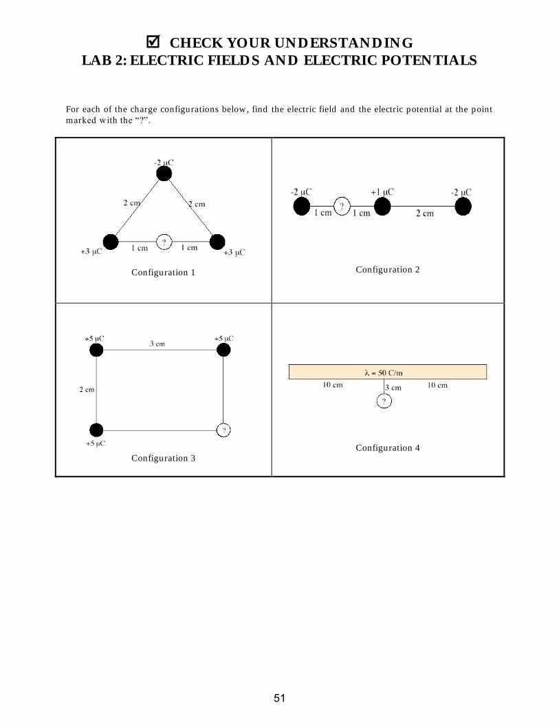
CHECK YOUR UNDERSTANDING
LAB 2: ELECTRIC FIELDS AND ELECTRIC POTENTIALS
For each of the charge configurations below, find the electric field and the electric potential at the point
marked with the “?”.
Configuration 1
Configuration 2
Configuration 3
Configuration 4
51

CHECK YOUR UNDERSTANDING
LAB 2: ELECTRIC FIELDS AND ELECTRIC POTENTIALS
52

Physics Lab Report Rubric
Name: ID#:Course, Lab Sequence, and Problem Number:Date Performed:Lab Partners’ Names:
Possible Earned
Warm-Up Questions
Possible Earned
Laboratory Notebook
Earns No Points Earns Full Points Possible EarnedArgument
• no clear argument• logic does not flow• gaps in content• leaves reader with questions
• complete, cogent, flowing argument• context, execution, analysis, conclu-
sion all present• leaves reader satisfied
Technical Style
• vocabulary, syntax, etc. inappropri-ate for scientific writing
• necessary nonverbal media absent orpoorly constructed
• subjective, fanciful, or appealing toemotions
• jarringly inconsistent
• language is appropriate• nonverbal media present where ap-
propriate, well constructed, well in-corporated
• objective, indicative, logical style• consistent style• division into sections is helpful
Use of Physics
• predictions with no or with unphysi-cal justification
• experiment physically unjustified• experiment tests wrong phenomenon• theory absent from consideration of
premise, predictions, and results
• predictions are justified with physicaltheory
• experiment is physically sound andactually tests phenomenon in ques-tion
• results interpreted with theory toclear, appropriate conclusion
Quantitativeness
• statements are vague or arbitrary• analysis is inappropriately qualitative• error analysis not used to evaluate
prediction or find result• numbers, equations, units, uncertain-
ties missing or inappropriate
• consistently quantitative• equations, numbers with units, uncer-
tainties throughout• prediction confirmed or denied, result
found by error analysis• results, conclusions based on data
Total
53

54

LAB 3: ELECTRIC ENERGY AND CAPACITORS
Our modern society functions in part because we have learned how to manipulate electrical energy. Almost all of our technology involves electrical energy in one form or another. In this laboratory you will investigate the conservation of energy as it relates to electricity. A capacitor is the simplest device that can store electrical energy. The problems in this lab involve transforming electrical energy stored in capacitors into light, kinetic energy, and other forms of energy that may be more difficult to detect. OBJECTIVES:
After successfully completing this laboratory, you should be able to:
Apply the concept of conservation of energy to solve problems involving electrical phenomena.
Describe the energy stored in a capacitor based on how it is connected to other capacitors and to sources of potential differences.
PREPARATION: Read Mazur Chapters 26 and 31. Before coming to lab you should be able to:
Calculate the work done by a force exerted on a moving object.
Calculate the relationship between power and energy.
Write the equation for the energy stored in a single capacitor and understand the meaning of all the quantities involved.
55

LAB 3: ELECTRIC ENERGY AND CAPACITORS
56

PROBLEM #1: ELECTRICAL AND MECHANICAL ENERGY
You have a job in a University research group investigating the effect of solar flares on the Earth’s magnetosphere. Your team is designing a small, cheap satellite for the investigation. As soon as the satellite achieves a stable orbit, it must extend its two solar panels. Your team must design a lightweight power source for deploying the solar panels. You have been asked to investigate the use of capacitors as a power source. You decide to calculate how the mechanical energy transferred to a device powered by a capacitor depends on the capacitance. You will test your calculation using a laboratory model in which a capacitor provides power to a motor that lifts a mass. You calculate how far the weight will move as a function of the capacitance of the capacitor. You assume that you know the initial voltage on the capacitor. Read: Mazur Sections 26.2 & 26.6 and review Section 5.7.
EQUIPMENT You have a mass set, a rod and clamps for securing the motor, string, several different capacitors, a battery or power supply, a meter stick, and a digital multimeter (DMM).
Read the section The Digital Multimeter (DMM) in the Equipment appendix. Read the appendices Significant Figures, Review of Graphs and Accuracy, Precision and Uncertainty to help you take data effectively. If equipment is missing or broken, submit a problem report by sending an email to [email protected]. Include the room number and brief description of the problem.
WARM UP
1. Draw pictures of the situation before the weight moves, while the weight is in motion, and after the weight has come to rest. Label all relevant distances, masses, forces, and potential differences. Describe the physics principles you need to solve this problem.
2. Define the initial and final times of interest in this problem. Describe (perhaps with your diagrams) what happens to energy in the situation between those times.
57

ELECTRICAL AND MECHANICAL ENERGY
3. Are there objects in the problem whose potential or kinetic energy is relevant, and whose energies you can calculate directly in terms of quantities measurable in the lab? If so, write down expressions for their initial and final (potential or kinetic) energies.
4. Use the work-energy theorem to write an equation for the net work done on the weight. Use this equation and equations from previous steps to write the amount of energy transferred from the capacitor to the weight during the entire lifting process, as a function of the distance the weight moves.
5. How would you define “efficiency” for this situation? Choose a system. Write an energy conservation equation for your system that relates the efficiency, the situation’s initial conditions, and properties you can measure in the lab, to the distance the weight moves.
6. Use the principle of energy conservation to write an equation for the amount of energy dissipated in this situation, in terms of measurable quantities and the efficiency. Be sure this equation is consistent with your description from step 2.
7. Sketch a graph of the distance the weight is lifted as a function of the capacitor’s capacitance. Assume constant efficiency, and that the capacitor is charged to the same potential difference for each trial. (You can check the “constant efficiency” assumption in the lab.)
PREDICTION Calculate the efficiency of the electric motor by determining the energy transferred from the capacitor and the final energy of the lifted mass.
EXPLORATION
WARNING: A charged capacitor can discharge quickly producing a painful spark. Do not handle the capacitors by their electrical terminals or connected wires by their metal ends. Always discharge a capacitor when you are finished using it. To discharge a capacitor, use an insulated wire to briefly connect one of the terminals to the other.
If you have not done so, read about using the DMM in the appendix. Pay special attention to the connections and settings that are used to measure voltages and currents, and why the DMM should be connected in the circuit differently for voltage and current measurements. Do you know why we should connect them in these ways? Note: Make sure you connect the + terminal of the battery to the + terminal of the capacitor! These capacitors are only designed to charge one way. If you connect the capacitors up the wrong way, the capacitance will change in an unpredictable manner.
58
ELECTRICAL AND MECHANICAL ENERGY
Charge the capacitor by connecting it to a battery. How can you use the DMM to tell if the capacitor is fully charged? What do you mean by fully charged? Try charging it for different amounts of time. How long does it take the capacitor to fully charge? Connect the mass to the motor with the string. Without touching the capacitor leads to anything else connect one lead to one terminal of the motor and the other lead to the other terminal of the motor. Which direction does the motor spin? Does the direction that the motor spins depend on how you connected the terminals to the motor? How far is the mass lifted? When the mass stops lifting is the capacitor out of energy? What implications does this have for your measurements? How long will the capacitor support the mass before it begins to fall? How can you tell when energy is still being transferred to the mass? What happens when energy is no longer being transferred to the mass? Write down your measurement plan.
MEASUREMENT What is the initial position of the mass? What is the energy stored in the capacitor at this time? Measure the distance the mass is lifted when the capacitor is connected to the motor. What was the energy of the capacitor at the final position? Was it necessary for the capacitor to be completely discharged at the final position? If it was not, what implications does this have for your experiment? What is more important, the total energy the capacitor is able to store, or the amount of energy the capacitor transfers? Is there a way you can visually determine that the capacitor is no longer transferring energy to the mass? What are the obvious changes to your system when energy is no longer being supplied to the mass from the capacitor? What are the uncertainties associated with your measurement? Try to think of any possible sources of uncertainty and quantify them.
ANALYSIS Graph the distance the weight is pulled versus the capacitance. Show the estimated measurement uncertainty on your graph.
59

ELECTRICAL AND MECHANICAL ENERGY
CONCLUSION
Did your results match your predictions? Explain any differences. How efficient is this energy transfer? Define what you mean by efficient. How good was the assumption of constant efficiency for this situation? You have heard that energy is always conserved. Is it appropriate to say that energy was conserved in this situation? Why or why not?
60

PROBLEM #2: SIMPLE CIRCUITS WITH CAPACITORS
You and your friend are trying to determine if you can use a capacitor to extend the lives of batteries in circuits. You suggest that you try a simple circuit with a capacitor, originally uncharged, connected to a battery through a switch. To monitor the output energy, you put a light bulb in series with the capacitor. Your friend believes that when the switch is closed the capacitor charges up and the bulb gets brighter and brighter until the brightness levels off. The bulb then stays on until the switch is opened. Do you agree? Read: Mazur Sections 31.1 – 31.2 & 31.6.
EQUIPMENT Build the circuit shown using of wires, bulbs, capacitors and batteries. Use the accompanying legend to help you build the circuit. You will also have a stopwatch and a digital multimeter (DMM).
Read the section The Digital Multimeter (DMM) in the Equipment appendix. If equipment is missing or broken, submit a problem report by sending an email to [email protected]. Include the room number and brief description of the problem.
PREDICTION Restate the problem. Do you agree with your friend? If not, describe what you think the behavior of the circuit will be. Give your reasoning. Explain what is going on in each component of the circuit. Sketch a qualitative graph of the bulb’s brightness vs. time.
EXPLORATION
WARNING: A charged capacitor can discharge quickly producing a painful spark. Do not handle the capacitors by their electrical terminals or connected wires by their metal ends. Always discharge a capacitor before you use it and when you are
61

SIMPLE CIRCUITS WITH CAPACITORS
finished using it. To discharge a capacitor, use an insulated wire to briefly connect one of the terminals to the other.
Examine each element of the circuit before you build it. How do you know if the battery is "good"? Is the capacitor charged? Carefully connect the two terminals of the capacitor to ensure it is uncharged. After you are convinced that all of the circuit elements are working and that the capacitor is uncharged, build the circuit but do not close it yet. Note: Make sure the + terminal of the battery or power supply is connected to the + terminal of the capacitor! These capacitors are only designed to charge one way. If you connect the capacitors up the wrong way, the capacitance will change in an unpredictable manner. Now, close the circuit and observe how the brightness of the bulb changes over time. From your observation of the bulb's brightness, how does the charge flowing through the bulb change over time? You can check this using the DMM set for current (Amps). See the Equipment appendix for instruction on the use of the DMM. Using a mental model of the capacitor as two parallel plates separated by a short distance, how does the charge accumulated on each plate of the capacitor change as the bulb’s brightness changes? Can you measure this with the DMM? Use conservation of charge to explain what you observe. From what you know about a battery, how does the potential difference (voltage) across the battery change over time? Check this using the DMM set for potential difference (Volts). From your observations of the brightness of the bulb, how does the potential difference across the bulb change over time? Check this using the DMM. What can you infer about the change of voltage (change of potential difference) across the capacitor over time? Can you check with a DMM? Use the concept of conservation of energy to explain what you observe. After a few moments, open the circuit. Is the capacitor charged or uncharged? To determine if the capacitor is charged, carefully (and safely) remove the battery from the circuit and reconnect the circuit without the battery. With only the capacitor and bulb (no battery) in the circuit, does the bulb light? Use the result to answer the following questions. Was the capacitor charged before you closed the circuit? Was the capacitor still charged long after the circuit was closed? Use conservation of charge and conservation of energy to explain your results.
62

SIMPLE CIRCUITS WITH CAPACITORS
CONCLUSION
Was your friend correct about how the brightness of the bulb changed? Sketch a qualitative graph of the brightness of the bulb as a function of time after you complete the circuit consisting of the initially discharged capacitor, battery and light bulb. How does this compare to your prediction? Sketch a qualitative graph of the charge on the capacitor as a function of time for this situation. Sketch a qualitative graph of the brightness of the bulb as a function of time after you complete the circuit consisting of the initially charged capacitor, NO battery and light bulb. Sketch a qualitative graph of the charge on the capacitor as a function of time for this situation. Describe how this graph relates to the changing potential difference across the capacitor, and to the changing amounts of charge on each plate of the capacitor.
63

SIMPLE CIRCUITS WITH CAPACITORS
64

PROBLEM #3: CAPACITANCE
You have a part time job as a special effects technician at a local theater. As part of the theatrical production, the play’s director wants a light bulb to dim very slowly for dramatic effect. You design a simple, inexpensive circuit to automatically accomplish this task: a battery, a switch, a light bulb, and a capacitor in series. You have been asked to demonstrate different rates of dimming for the light bulb so the director can select the one that best fits the performance. You need to determine how to adjust the amount of time it takes for the light bulb to go out by varying the capacitance. To make a proper comparison you make sure that the capacitor is initially uncharged. Read: Mazur Sections 31.1 – 31.2 & 31.6.
EQUIPMENT Build the circuit shown; you have a choice of capacitors. You will also have a stopwatch and a digital multimeter (DMM). Use the accompanying legend to help you build the circuit.
Read the section The Digital Multimeter (DMM) in the Equipment appendix. If equipment is missing or broken, submit a problem report by sending an email to [email protected]. Include the room number and brief description of the problem.
PREDICTION Restate the problem. What is the quantity you will be measuring and what is the quantity you will be controlling? How do you think they will depend on one another? Give your reasoning. Explain what is going on in each component of the circuit. Sketch a graph of the time it takes for the light bulb to turn completely off as a function of the capacitor’s capacitance.
EXPLORATION
WARNING: A charged capacitor can discharge quickly producing a painful spark. Do not handle the capacitors by their electrical terminals or connected wires by their metal ends. Always discharge a capacitor before you use it and when you are finished using it. To discharge a capacitor, use an insulated wire to briefly connect one of the terminals
65
CAPACITANCE
to the other. Examine each element of the circuit before you build it. How do you know if the battery is "good"? Be sure the capacitors are uncharged. After you are convinced that all of the circuit elements are working and that the capacitor is uncharged, connect the circuit but do not close it yet. Note: Make sure the + terminal of the battery is connected to the + terminal of the capacitor! These capacitors are only designed to charge one way. If you connect the capacitors up the wrong way, the capacitance will change in an unpredictable manner. Now, close the circuit and observe how the brightness of the bulb changes over time. How long does it take for the bulb to turn off? From what you know about a battery, how does the potential difference (voltage) across the battery change over time? Check this using the DMM set for potential difference (Volts). From your observations of the brightness of the bulb, how does the potential difference across the bulb change over time? Check this using the DMM. What can you infer about the change of voltage across the capacitor over time? Can you check with a DMM? Use the concept of potential difference to explain what you observe. Develop a measurement plan that will allow you to determine the time it takes a bulb to turn off as a function of capacitance. You will want to decide how many different capacitors you need to use, how many time measurements to take for each capacitor, what you mean by the light bulb being “off,” and how to ensure that the capacitor is uncharged before you make each measurement.
MEASUREMENT Follow your measurement plan. Be sure to record your estimated uncertainty for each measurement.
ANALYSIS Graph the time it takes for the light bulb to turn off, as a function of capacitance, with the capacitor initially uncharged.
CONCLUSION How did your measurement compare with your prediction? Using conservation of charge, conservation of energy, and the model of a capacitor as two plates separated by a short distance, explain how the capacitance affects the time it takes for the bulb to turn off.
66
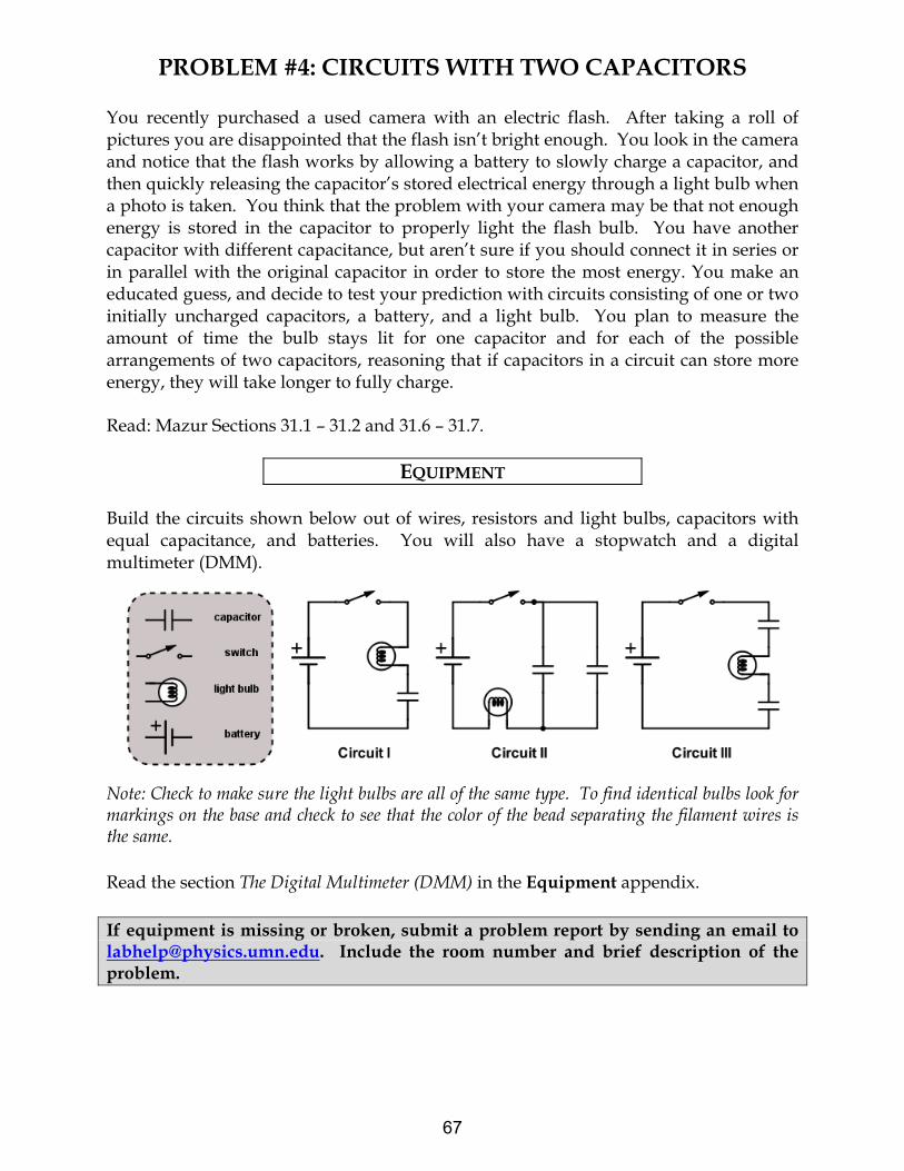
PROBLEM #4: CIRCUITS WITH TWO CAPACITORS
You recently purchased a used camera with an electric flash. After taking a roll of pictures you are disappointed that the flash isn’t bright enough. You look in the camera and notice that the flash works by allowing a battery to slowly charge a capacitor, and then quickly releasing the capacitor’s stored electrical energy through a light bulb when a photo is taken. You think that the problem with your camera may be that not enough energy is stored in the capacitor to properly light the flash bulb. You have another capacitor with different capacitance, but aren’t sure if you should connect it in series or in parallel with the original capacitor in order to store the most energy. You make an educated guess, and decide to test your prediction with circuits consisting of one or two initially uncharged capacitors, a battery, and a light bulb. You plan to measure the amount of time the bulb stays lit for one capacitor and for each of the possible arrangements of two capacitors, reasoning that if capacitors in a circuit can store more energy, they will take longer to fully charge. Read: Mazur Sections 31.1 – 31.2 and 31.6 – 31.7.
EQUIPMENT Build the circuits shown below out of wires, resistors and light bulbs, capacitors with equal capacitance, and batteries. You will also have a stopwatch and a digital multimeter (DMM).
Note: Check to make sure the light bulbs are all of the same type. To find identical bulbs look for markings on the base and check to see that the color of the bead separating the filament wires is the same. Read the section The Digital Multimeter (DMM) in the Equipment appendix.
If equipment is missing or broken, submit a problem report by sending an email to [email protected]. Include the room number and brief description of the problem.
67
CIRCUITS WITH TWO CAPACITORS
WARM UP
1. Draw a picture of each arrangement of the capacitors, light bulb, and battery. On each picture, label the capacitance of each capacitor. (Remember that you will have capacitors with different capacitances.) Also, label the electric potential difference across each circuit element and the charge stored on the plates of each capacitor.
2. Decide on the physics principles you will use. For a circuit, conservation of charge is usually useful, as is conservation of energy. What is the relationship between the total energy stored in each circuit and the energy stored on each capacitor in that circuit?
3. For each capacitor, determine an equation that relates its stored energy, the charge collected on its plates, and its capacitance.
4. For each capacitor, write an equation relating the charge on its plates, the potential difference across the capacitor, and its capacitance.
5. After the current stops flowing through the circuit, do the two capacitors in Circuit II have the same amount of stored charge? Circuit III? At that time, what is the potential difference across the bulb in each circuit? At that time, what is the relationship between the potential difference across the battery and the potential difference across each capacitor?
6. The target quantity is the energy stored in the capacitors of each circuit. To determine which circuit stores more energy in the capacitors, you must calculate the energy stored in terms of quantities you can easily find, such as the potential difference across the battery and the capacitance of each capacitor.
7. From the previous steps, you can find the total energy stored in the capacitors in each circuit in terms of the potential difference across the battery and the capacitance of each capacitor. Now compare them to determine which is largest. Check your equations by making the comparison when both capacitors have the same capacitance. Does the result make sense?
8. What assumptions must you make to relate the total energy stored in the capacitors for each configuration to the time the light bulb remains lit after each circuit is closed?
PREDICTION
Restate the problem. What quantity do you wish to compare across the three situations? Use physics to decide how they will compare. Which quantity will you be measuring directly? Describe qualitatively how it is connected to the quantity of interest.
68
CIRCUITS WITH TWO CAPACITORS
EXPLORATION
WARNING: A charged capacitor can discharge quickly producing a painful spark. Do not handle the capacitors by their electrical terminals or connected wires by their metal ends. Always discharge a capacitor before you use it and when you are finished using it. To discharge a capacitor, use an insulated wire to briefly connect one of the terminals to the other.
Make sure all of your capacitors are uncharged before starting the exploration. Examine each element of the circuit before you build it. How do you know if the battery and the bulb are "good"? Connect Circuit I to use as a reference. Note: Make sure the + terminal of the battery is connected to the + terminal of the capacitor! These capacitors are only designed to charge one way. If you connect the capacitors up the wrong way, the capacitance will change in an unpredictable manner. Close the circuit and observe how the brightness of the bulb changes over time. How long does it take for the bulb to turn off? Connect Circuit II using the capacitor from Circuit I along with a capacitor with a different capacitance. Do not close the circuit yet. Do you think the bulb will light when the circuit is closed? Record your reasoning in your journal. Now, close the circuit. Record your observations and explain what you saw using conservation of charge and the concept of potential difference. Does the order that you connect the two capacitors and the bulb in the circuit matter? Try following one capacitor with the other capacitor and then the bulb. Try switching the two capacitors. When the brightness of the bulb no longer changes, how are the the potential differences across the circuit elements related? Check this using the DMM, set for potential difference (Volts). Use the concept of energy conservation to explain what you observe. Connect Circuit III using the two capacitors you used in Circuit II. Do not close the circuit yet. Do you think the bulb will light when the circuit is closed? Record your reasoning in your journal. Now, close the circuit. Record your observations and explain what you saw using conservation of charge and the concept of potential difference. Use the DMM to check the relationship between the potential differences across the elements of this circuit. Explain what you observe. Develop a plan for measuring the time that it takes for the bulbs in Circuits I, II, and III to turn off, if they light at all.
69

CIRCUITS WITH TWO CAPACITORS
MEASUREMENT
Use your measurement plan to record how long it takes for the light bulb to go off for each circuit. Use “0 seconds” for any bulbs that did not light. What are the uncertainties in these measurements?
ANALYSIS Rank the actual time it took each bulb to turn off. Do all the bulbs initially light? Do all the bulbs eventually go off?
CONCLUSION How did your initial ranking of the time it would take for the bulbs to go out compare with what actually occurred? Use conservation of charge, conservation of energy, and the concept of potential difference to explain your results. Compare the reasoning you used in the exploration section to predict whether the bulbs would light in each circuit to the understanding you now have. If your reasoning has changed, explain why it changed.
70

CHECK YOUR UNDERSTANDING LAB 3: ELECTRICAL ENERGY AND CAPACITORS
For each of the arrangements of identical capacitors shown below:
1) Rank them in terms of the amount of time they can light a light bulb. Assume that the leads shown have been connected to a 6 Volt battery and then removed from the battery and connected to a light bulb.
2) Calculate the potential difference between the terminals of each capacitor. Assume that the leads
shown have been connected to a 6 Volt battery and that the capacitance of each capacitor is 10 F.
3) Calculate the amount of energy stored in each capacitor and the total energy stored in each arrangement of capacitors. Assume that the leads shown have been connected to a 6 Volt battery and that the capacitance of each capacitor is 10 F.
71

CHECK YOUR UNDERSTANDING LAB 3: ELECTRICAL ENERGY AND CAPACITORS
72

Physics Lab Report Rubric
Name: ID#:Course, Lab Sequence, and Problem Number:Date Performed:Lab Partners’ Names:
Possible Earned
Warm-Up Questions
Possible Earned
Laboratory Notebook
Earns No Points Earns Full Points Possible EarnedArgument
• no clear argument• logic does not flow• gaps in content• leaves reader with questions
• complete, cogent, flowing argument• context, execution, analysis, conclu-
sion all present• leaves reader satisfied
Technical Style
• vocabulary, syntax, etc. inappropri-ate for scientific writing
• necessary nonverbal media absent orpoorly constructed
• subjective, fanciful, or appealing toemotions
• jarringly inconsistent
• language is appropriate• nonverbal media present where ap-
propriate, well constructed, well in-corporated
• objective, indicative, logical style• consistent style• division into sections is helpful
Use of Physics
• predictions with no or with unphysi-cal justification
• experiment physically unjustified• experiment tests wrong phenomenon• theory absent from consideration of
premise, predictions, and results
• predictions are justified with physicaltheory
• experiment is physically sound andactually tests phenomenon in ques-tion
• results interpreted with theory toclear, appropriate conclusion
Quantitativeness
• statements are vague or arbitrary• analysis is inappropriately qualitative• error analysis not used to evaluate
prediction or find result• numbers, equations, units, uncertain-
ties missing or inappropriate
• consistently quantitative• equations, numbers with units, uncer-
tainties throughout• prediction confirmed or denied, result
found by error analysis• results, conclusions based on data
Total
73

74
LAB 4: ELECTRIC CIRCUITS
In the first laboratory, you studied the behavior of electric fields and their effect on the motion of electrons using a cathode ray tube (CRT). This beam of electrons is one example of an electric current – charges in motion. The current in the CRT was simple in that the electrons moved through a vacuum. The forces on them were completely known. Their behavior could be determined by calculating the electric field and then applying kinematics. In contrast to the CRT, common electric currents are inside materials such as wires or light bulbs. Even though the interactions of electrons inside materials are quite complicated, the basic principles of physics still apply. Conservation of energy and charge allow us to determine the overall behavior of electric currents without the need to know the details of the electrons’ interactions. This approach to problem solving in the realm of electric circuits will give you more experience in applying the very useful principles of conservation. OBJECTIVES After successfully completing this laboratory, you should be able to:
Apply the concepts of circuits to electrical systems.
Apply the concept of conservation of charge to determine the behavior of the electrical current through any part of a circuit.
Apply the concept of conservation of energy to determine the behavior of the energy output of any element in a circuit.
Use the concept of electric potential to describe the behavior of a circuit.
Relate the electric charge on a circuit element to the potential difference across that element and the capacitance of that element.
Relate the electric current through a circuit element to the resistance of that element and potential difference across that element.
Measure the current through a circuit element with a digital multimeter (DMM).
Measure the voltage between two points in a circuit with a DMM.
Measure the resistance of a circuit element with a DMM. PREPARATION Read Mazur Chapter 31. It is likely that you will be doing these laboratory problems before your lecturer addresses this material. The purpose of this laboratory is to give you these experiences
75

LAB 4: ELECTRIC CIRCUITS
as an introduction to the material. So, it is very important that, when you read the text before coming to lab, you remember the objectives of the laboratory. Before coming to lab you should be able to:
Describe the relationship between charge and current.
Describe the relationship between potential and potential energy.
Describe the essential difference between an insulator and a conductor.
Identify what is an electrical circuit and what is not.
Apply conservation of energy and conservation of charge to current flowing around a circuit.
Write down Ohm's law and know when to apply it.
Describe the difference between a capacitor, a resistor, and a battery.
Use a DMM to measure potential difference, current, and resistance.
76

PROBLEM #1: SIMPLE CIRCUITS
You need more light in your workroom, so you decide to add another light fixture to your track lighting. However, you are concerned that adding another light may dim the lights that are already in the track. When you proceed with the addition of another light, you notice that none of the lights are dimmer than before. You wonder what type of circuit your track lighting uses. You decide to build models of circuits with two bulbs connected across a battery, and to compare the brightness of the bulbs in these circuits to a reference circuit with a single bulb. The circuit in which each bulb is as bright as the one in your reference circuit is the same type as the circuit in your track lighting. Read: Mazur Sections 31.3 and 31.6 – 31.7.
EQUIPMENT You will build three simple circuits shown below out of wires, bulbs, and batteries. Use the accompanying legend to build the circuits.
Note: Check to make sure the light bulbs are all of the same type. To find identical bulbs look for markings on the base and check to see that the color of the bead separating the filament wires is the same. If equipment is missing or broken, submit a problem report by sending an email to [email protected]. Include the room number and brief description of the problem.
PREDICTION Restate the problem. Rank, in order of brightness, the bulbs A, B, C, D, and E from the brightest to the dimmest (use the symbol ‘=’ for "same brightness as" and the symbol ‘ >’ for "brighter than"). Write down your reasoning.
77

SIMPLE CIRCUITS
EXPLORATION
Reference Circuit I Connect Circuit I to use as a reference. Observe the brightness of bulb A. Replace the bulb with another one and again observe the brightness. Repeat until you have determined the brightness of all your bulbs when they are connected into the same type of circuit. If the bulbs are identical, they should have the same brightness. Note: Pay attention to large differences you may observe, rather than minor differences that may occur if two "identical" bulbs are, in fact, not quite identical. How can you test whether minor differences are due to manufacturing irregularities? Circuit II Connect Circuit II. Compare the brightness of bulbs B and C. What can you conclude from this observation about the amount of current through each bulb? Is current "used up" in the first bulb, or is the current the same through both bulbs? Try switching bulbs B and C. Based on your observation, what can you infer about the current at points 1, 2, and 3? How does the brightness of bulb A (Circuit I) compare to the brightness of bulbs B and C (Circuit II)? What can you infer about the current at point 1 in each of the two circuits? Circuit III Connect Circuit III. Compare the brightness of bulbs D and E. What can you conclude from this observation about the amount of current through each bulb? Describe the flow of current around the entire circuit. What do your observations suggest about the way the current through the battery divides and recombines at junctions where the circuit splits into two branches? How does the current at point 1 compare with the currents at points 2 and 3? How does the brightness of bulb A (Circuit I) compare to the brightness of bulbs D and E (Circuit III)? What can you infer about the current at point 1 in each of the two circuits? Comparing the three circuits, does the amount of current at point 1 appear to remain constant or to depend on the number of bulbs and how they are connected?
78

SIMPLE CIRCUITS
CONCLUSION
Rank the actual brightness of the bulbs. How did this compare to your prediction? Make sure you adequately describe what you mean in your comparisons, i.e. “the same brightness as”, “brighter than”, “dimmer than”. What type of circuit is used in your track lighting? Circuit II is called a series circuit and Circuit III is called a parallel circuit. Can you use conservation of energy and conservation of current to explain your results? The rate that energy is output from a bulb is equal to the potential difference (voltage) across the bulb times the current through the bulb. Does a battery supply a constant current or a constant potential difference to circuits? To check your understanding, rank the brightness of the bulbs in the following circuits. Use the lab equipment to see if your answer is correct.
79

SIMPLE CIRCUITS
80
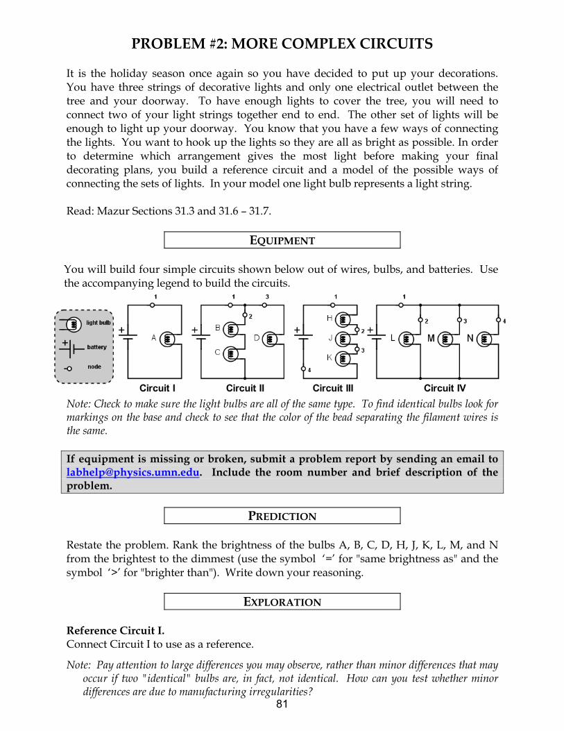
PROBLEM #2: MORE COMPLEX CIRCUITS
It is the holiday season once again so you have decided to put up your decorations. You have three strings of decorative lights and only one electrical outlet between the tree and your doorway. To have enough lights to cover the tree, you will need to connect two of your light strings together end to end. The other set of lights will be enough to light up your doorway. You know that you have a few ways of connecting the lights. You want to hook up the lights so they are all as bright as possible. In order to determine which arrangement gives the most light before making your final decorating plans, you build a reference circuit and a model of the possible ways of connecting the sets of lights. In your model one light bulb represents a light string. Read: Mazur Sections 31.3 and 31.6 – 31.7.
EQUIPMENT You will build four simple circuits shown below out of wires, bulbs, and batteries. Use the accompanying legend to build the circuits.
Note: Check to make sure the light bulbs are all of the same type. To find identical bulbs look for markings on the base and check to see that the color of the bead separating the filament wires is the same. If equipment is missing or broken, submit a problem report by sending an email to [email protected]. Include the room number and brief description of the problem.
PREDICTION Restate the problem. Rank the brightness of the bulbs A, B, C, D, H, J, K, L, M, and N from the brightest to the dimmest (use the symbol ‘=’ for "same brightness as" and the symbol ‘>’ for "brighter than"). Write down your reasoning.
EXPLORATION Reference Circuit I. Connect Circuit I to use as a reference.
Note: Pay attention to large differences you may observe, rather than minor differences that may occur if two "identical" bulbs are, in fact, not identical. How can you test whether minor differences are due to manufacturing irregularities?
81

MORE COMPLEX CIRCUITS
Circuit II Connect Circuit II. Compare the brightness of bulbs B and C. Compare the brightness of bulbs B and C to bulb D. What can you conclude from this observation about the amount of current through each bulb? How does the brightness of bulbs B and C compare to the brightness of bulb A (Circuit I)? What can you infer about the current at point 2 in Circuit II and the current at point 1 in Circuit I? How does the brightness of bulb D compare to the brightness of bulb A (Circuit I)? What can you infer about the current at point 3 in Circuit II and the current at point 1 in Circuit I? Describe the flow of current around the entire circuit. What do your observations suggest about the way the current through the battery divides and recombines at junctions where the circuit splits into two parallel branches? How does the current at point 1 in Circuit II compare with the current at point 1 in Circuit I? Explain any differences. Circuit III. Connect Circuit III. Compare the brightness of the bulbs. What can you conclude from this observation about the amount of current through each bulb? How does the brightness of bulb H compare to the brightness of bulb A (Circuit I)? What can you infer about the current at point 1 in Circuit III and the current at point 1 in Circuit I? Circuit IV. Connect Circuit IV. Compare the brightness of the bulbs. What can you conclude from this observation about the amount of current through each bulb? How does the brightness of bulb L compare to the brightness of bulb A (Circuit I)? What can you infer about the current at point 1 in Circuit IV and the current at point 1 in Circuit I?
CONCLUSION Rank the actual brightness of the bulbs A, B, C, D, H, J, K, L, M and N. Make sure you have adequately defined your comparisons: “same brightness as”, “brighter than”, and “dimmer than”. How did your prediction compare to your results? Can you use conservation of energy and conservation of current to explain your results? How will you connect your three strings of lights so that they are all as bright as possible?
82

PROBLEM #3: SHORT CIRCUITS
A friend of yours who manages a movie theater is having a problem with the lights that surround the marquee. Some of the light bulbs don’t light up. But when he takes out the bulbs and checks them individually, they all work. You tell him he must have a short circuit. You explain that you have a short circuit when a wire makes an alternate path for the current to bypass a circuit element. To demonstrate this idea, you build a few simple circuits to show the results of a short circuit. Read: Mazur Sections 31.3 and 31.6 – 31.7.
EQUIPMENT You will build three simple circuits shown below out of wires, bulbs, and batteries. Use the accompanying legend to build the circuits.
Note: Make sure that you are using identical light bulbs. Look for markings on the base of the bulb and check to see that the color of the bead separating the filament wires is the same. If equipment is missing or broken, submit a problem report by sending an email to [email protected]. Include the room number and brief description of the problem.
PREDICTION Restate the problem. Circuit II: What happens to the brightness of bulbs B and C when a wire is attached across bulb B (from point 1 to point 2)? Circuit III: What happens to the brightness of bulbs D and E when a wire is attached across bulb E? Circuit I: What happens to the brightness of the bulb A when a wire is attached across the bulb?
83
SHORT CIRCUITS
EXPLORATION
WARNING: A short circuit is what happens any time a very low-resistance path (like a wire, or other piece of metal) is provided between points in a circuit that are at different potentials, like the terminals of a battery or power supply. Short circuits can destroy equipment and injure people! Always avoid short circuits in other circuits! Short circuits damage equipment by causing larger currents in a circuit than they are designed for. Only apply the short circuit for a small amount of time.
Build Circuit II. What happens to the brightness of bulbs B and C when you place a wire across bulb B? How did the current through C change? How did the current through B change? Did the current through point 1 change? If so, in what way? Did the wire across bulb B get warmer? Explain your answers. Build Circuit III. What happens to the brightness of bulbs D and E when you place a wire across bulb E? Did the current through D change? Did the current through E change? Did the wire across bulb E get warm? What would be the brightness of a bulb inserted in the circuit at point 1? Explain your answers. Build Circuit I. Place a wire across the bulb. What happens to the brightness of the bulb? Hold on to the wire that is across the bulb. Is it getting warmer? How did the current through the bulb change? How about the current coming out of the battery? Make sure you disconnect the battery when you are done. Placing the wire across the bulb causes a short circuit and it is called "shorting out" the bulb.
CONCLUSIONS Did your predictions match your observed results? What have you learned from experiments, which agreed with your predictions? Draw more conclusions based on the experiments where your predictions were different from what you observed.
84
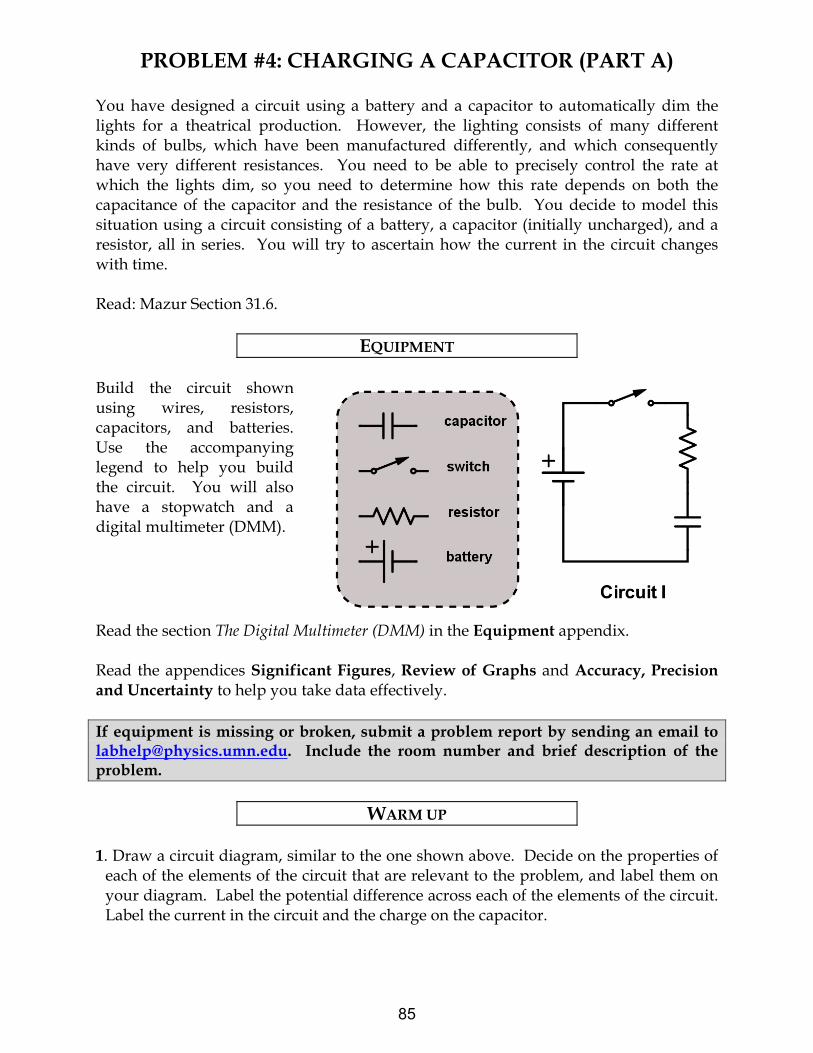
PROBLEM #4: CHARGING A CAPACITOR (PART A)
You have designed a circuit using a battery and a capacitor to automatically dim the lights for a theatrical production. However, the lighting consists of many different kinds of bulbs, which have been manufactured differently, and which consequently have very different resistances. You need to be able to precisely control the rate at which the lights dim, so you need to determine how this rate depends on both the capacitance of the capacitor and the resistance of the bulb. You decide to model this situation using a circuit consisting of a battery, a capacitor (initially uncharged), and a resistor, all in series. You will try to ascertain how the current in the circuit changes with time. Read: Mazur Section 31.6.
EQUIPMENT Build the circuit shown using wires, resistors, capacitors, and batteries. Use the accompanying legend to help you build the circuit. You will also have a stopwatch and a digital multimeter (DMM).
Read the section The Digital Multimeter (DMM) in the Equipment appendix. Read the appendices Significant Figures, Review of Graphs and Accuracy, Precision and Uncertainty to help you take data effectively. If equipment is missing or broken, submit a problem report by sending an email to [email protected]. Include the room number and brief description of the problem.
WARM UP 1. Draw a circuit diagram, similar to the one shown above. Decide on the properties of
each of the elements of the circuit that are relevant to the problem, and label them on your diagram. Label the potential difference across each of the elements of the circuit. Label the current in the circuit and the charge on the capacitor.
85

CHARGING A CAPACITOR (PART A)
2. Use energy conservation to write an equation relating the potential differences across all elements of the circuit. Write an equation relating the potential difference across the capacitor plates and the charge stored on its plates. What is the relationship between the current through the resistor and the voltage across it? Are these three equations always true, or only for specific times?
3. Describe qualitatively how each quantity labeled on your diagram changes with time.
What is the voltage across each element of the circuit (a) at the instant the circuit is closed; (b) when the capacitor is fully charged? What is the current in the circuit at these two times? What is the charge on the capacitor plates at these two times?
4. From the equations you constructed above, determine an equation relating the
voltage of the battery, the capacitance of the capacitor, the resistance of the resistor, the current through the circuit, and the charge stored on the capacitor plates.
5. Write an equation relating the rate of charge accumulation on the capacitor plates to
the current through the circuit. 6. Use the equations you have written to get a single equation that relates the current
and the rate of change of current to the known properties of each circuit element. To do this, you may find it helpful to differentiate one of your equations.
7. Solve the equation from step 6 by using one of the following techniques: (a) Guess the
current as a function of time, which satisfies the equation, and check it by substituting your current function into your equation; (b) Get all the terms involving current on one side of the equation and time on the other side and solve. Solving the equation may require an integral.
8. Complete your solution by determining any arbitrary constants in your solution,
using the initial value of the current you obtained in question 3.
PREDICTION When the circuit is closed, with the capacitor initially uncharged, how does the current in the circuit change with time? How long does it take for the current to fall to zero? Sketch a graph of current against time for this circuit, assuming the capacitor is initially uncharged.
86
CHARGING A CAPACITOR (PART A)
EXPLORATION
WARNING: A charged capacitor can discharge quickly producing a painful spark. Do not handle the capacitors by their electrical terminals or connected wires by their metal ends. Always discharge a capacitor when you are finished using it. To discharge a capacitor, use an insulated wire to briefly connect one of the terminals to the other.
If you have not done so, read about using the DMM in the Equipment appendix. Pay special attention to the connections and settings that are used to measure voltages and currents, and why the DMM should be connected in the circuit differently for voltage and current measurements. Do you know why we should connect them in these ways? Note: Make sure the + terminal of the battery is connected to the + terminal of the capacitor! These capacitors are only designed to charge one way. If you connect the capacitors up the wrong way, the capacitance will change in an unpredictable manner. Examine each element of the Circuit I before you build it. Is the capacitor charged? Carefully connect the two terminals of the capacitor to ensure it is uncharged. How can you determine the resistance of the resistor? Is there a way to confirm it? After you are convinced that all of the circuit elements are working and that the capacitor is uncharged, build the circuit with a light bulb in place of the resistor, but leave the circuit open. Close the circuit and observe how the brightness of the bulb changes with time. What can you infer about the way the current in the circuit changes with time? From what you know about a battery, how does the potential difference (voltage) across the battery change over time? Check this using the DMM set for potential difference (Volts). From your observations of the brightness of the bulb, how does the potential difference across the bulb change over time? Check this using the DMM. What can you infer about the change of voltage across the capacitor over time? Can you check with a DMM? Use the concept of potential difference to explain what you observe. Now, discharge the capacitor, and reconnect the DMM in such a way that it measures the current in the circuit. Close the circuit and observe how the current changes with time? Is it as you expected? How long does it take for the current to fall to zero? Replace the light bulb with a resistor. Qualitatively, how will changing the resistance of the resistor and the capacitance of the capacitor affect the way the current in the circuit changes with time? How can you test this experimentally?
87

CHARGING A CAPACITOR (PART A)
Build the circuit, including a DMM in the circuit to measure the current. Close the circuit and observe how long it takes for the current in the circuit to halve. How does changing the capacitance of the capacitor or the resistance of the resistor affect this time? Choose a capacitor value and a range of resistances that allow you to most effectively construct a graph to test your prediction. Complete your measurement plan.
MEASUREMENT Measure the current flowing through the circuit for as many times as you deem necessary. Make your measurements using a resistor, not a bulb. What are the uncertainties in each of these measurements?
ANALYSIS Use your measured values for the resistance of the resistor, the capacitance of the capacitor, and the voltage of the battery, along with your prediction equation, to construct a graph of your predicted current against time. Make a graph of the measured current flowing through the circuit against time. Compare these two graphs, noting any similarities and explaining any differences.
CONCLUSION Describe which of your predictions were confirmed by experiments and draw conclusions accordingly. To continue conclusions, explain what was incorrect in those of your predictions that your laboratory observations or measurements did not support (or what went wrong with the experiment that failed to verify your prediction). Finally, use theory and your experimental results from this problem to answer the following question: Does the current in the circuit change linearly with time?
88

PROBLEM #5: CIRCUITS WITH TWO CAPACITORS
You are modifying the design of a sturdy, low-cost beeper to be used as a safety device on children’s bicycles. The sound-producing component of the beeper will not pass current or make noise until after the potential difference across it reaches a certain value. This component is connected in parallel to the capacitor in an RC circuit. When the threshold voltage is reached, the capacitor discharges through the sound-producing component, and then begins to charge again. The time between beeps is thus determined by the time it takes for the capacitor to charge to a certain value. You wish to shorten the amount of time between beeps and decide to modify the capacitance. You don’t want to buy new capacitors because the original ones are extremely cheap and reliable. You decide to use two of the original capacitors for each beeper. There are at least two different ways to arrange the capacitors in the circuit: in series with each other, or in parallel. How would you arrange the capacitors in order to reduce the time between beeps? In order to understand the quantitative behavior of each circuit, you decide to make some measurements on the circuits with the sound emitter removed. Read: Mazur Sections 31.6 – 31.7.
EQUIPMENT You will build the circuits shown below out of wires, resistors, 2 uncharged capacitors of equal capacitances, and a battery. To visualize the presence of electric current in the circuits, you will replace resistors with light bulbs. (Note, however, that you cannot fairly compare capacitances in the circuits unless the bulbs are identical. Using the same bulb in all circuits is a possible way to ensure that.) You will have a stopwatch and a digital multimeter (DMM) for measurements.
Read the section The Digital Multimeter (DMM) in the Equipment appendix. Read the appendices Significant Figures, Review of Graphs and Accuracy, Precision and Uncertainty to help you take data effectively. If equipment is missing or broken, submit a problem report by sending an email to [email protected]. Include the room number and brief description of the problem. If you are unable to, ask your TA to submit a problem report.
89

CIRCUITS WITH TWO CAPACITORS
WARM UP
1. For each of the circuits, draw a circuit diagram, similar to those shown above. Decide on the properties of each of the elements of the circuit that are relevant to the problem, and label them on your diagram. Label the potential difference across each of the elements of the circuit. Label the current in the circuit and the charge on each capacitor. What is the relationship between the charges on the two capacitors of Circuit II? What about the two capacitors of Circuit III? Under what conditions will the bulb go out?
2. Write an equation relating the potential difference across each of the elements of the circuit. What is the relationship between the potential difference across the plates of each capacitor and the charge stored on its plates? What is the relationship between the current through a resistor (in the place of each bulb) and the voltage across it? Are these equations always true, or only for specific times?
3. Explain how each of the quantities labeled on your diagram changes with time. What is the voltage across each of the elements of the circuit (a) at the instant the circuit is closed, (b) when the capacitor is fully charged? What is the current through the resistor at these two times? What is the charge on each of the capacitors at these two times?
4. From the equations you constructed above, determine an equation relating the voltage of the battery, the capacitance of each of the capacitors, the resistance of the resistor, the current through the resistor, and the charge stored on each of the capacitors.
5. Write an equation relating the rate of charge accumulation on the capacitor plates to the current through the circuit.
6. Use the equations you have written to get a single equation that relates the current and the rate of change of current to the known properties of each circuit element. To do this, you may find it helpful to differentiate one of your equations.
7. Solve the equation from step 6 by using one of the following techniques: (a) Guess the current as a function of time, which satisfies the equation, and check it; (b) Get all the terms involving current on one side of the equation and time on the other side and solve. Solving the equation may require an integral.
8. Complete your solution by determining any arbitrary constants in your solution, using the initial value of the current obtained above.
Repeat the above steps for the other two circuits.
PREDICTION
90
CIRCUITS WITH TWO CAPACITORS
For each of Circuits I, II, and III, draw a graph to qualitatively describe the current through the resistor (or the light bulb) as a function of time after the switch is closed, if the capacitors are initially uncharged. Compare the times it will take for light bulbs to go off in each circuit. For the comparison to be fair, do you think it is important that in each circuit (i) The resistances of light bulbs are the same, and (ii) The light bulb is connected in series with the battery? Having made necessary assumptions for a fair comparison, rank Circuits I, II, and III by the time it will take for the bulbs to go off.
EXPLORATION
WARNING: A charged capacitor can discharge quickly producing a painful spark. Do not handle the capacitors by their electrical terminals or connected wires by their metal ends. Always discharge a capacitor before you use it and when you are finished using it. Review your exploration from the earlier problem, Charging a Capacitor (PartA). Before you start building a circuit, examine each element of it. How do you know if the battery is "good"? Are the capacitors charged? Carefully connect the two terminals of each capacitor to ensure it is uncharged. Make sure you that have two capacitors of the same capacitance. Note: Make sure the + terminal of the battery is connected to the + terminal of the capacitor! These capacitors are only designed to charge one way. If you connect the capacitors up the wrong way, the capacitance will change in an unpredictable manner. Check that the polarity of the capacitor’s connection is correct and begin your observations by using bulbs instead of resistors. Build Circuit I, but do not close the switch. Do you think the bulb will light when the circuit is closed? Record your reasoning in your journal. Close the circuit. Record your observations and explain what you saw using conservation of charge and the concept of potential difference. Build Circuit II, but do not close the switch. Do you think the bulb will light when the circuit is closed? Record your reasoning in your journal. Close the circuit. Record your observations and explain what you saw using conservation of charge and the concept of potential difference. Does it make a difference if you put the bulb in series with of one of the capacitors?
91
CIRCUITS WITH TWO CAPACITORS
Build Circuit III, but do not close the switch. Do you think the bulb will light when the circuit is closed? Record your reasoning in your journal. Close the circuit. Record your observations and explain what you saw using conservation of charge and the concept of potential difference. Does the order in which you connect the two capacitors and the bulb in the circuit matter? Try following one capacitor with the other capacitor and then the bulb. Now, replace the light bulbs in your circuits with resistors. How can you determine the resistance of the resistor? Is there a way to confirm it? Connect a DMM in each of the circuits and observe how the current changes with time. For each circuit, decide how many measurements you will need to make in order to make a graph of current against time, and what time interval between measurements you will choose. Complete your measurement plan.
MEASUREMENT Measure the current in each circuit for as many different times as you deem necessary. Make your measurements using resistors, not bulbs. What are the uncertainties in each of these measurements?
ANALYSIS Use your measurements to plot the (measured) values of current as a function of time for circuits I, II, and III.
CONCLUSION How well did your graphs drawn from your data compare to those in your predictions? Explain any differences. How did your predicted rankings of the time each bulb would remain lit compare to your measurements? Explain any differences.
92
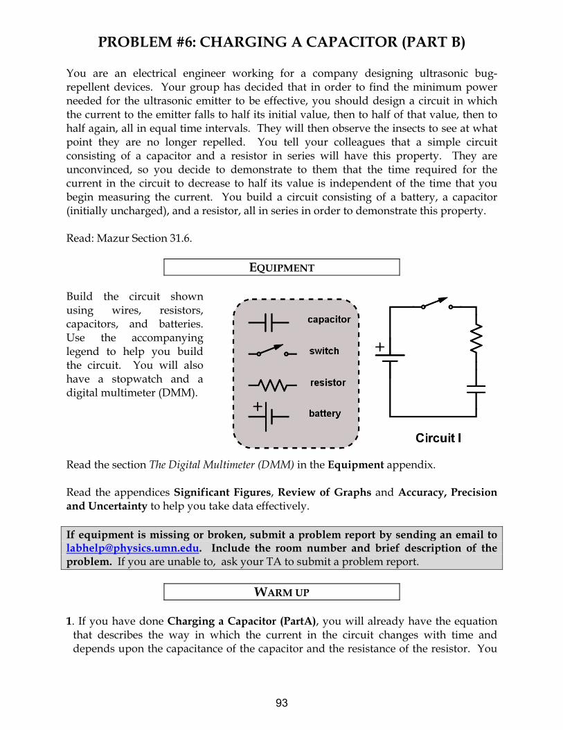
PROBLEM #6: CHARGING A CAPACITOR (PART B)
You are an electrical engineer working for a company designing ultrasonic bug-repellent devices. Your group has decided that in order to find the minimum power needed for the ultrasonic emitter to be effective, you should design a circuit in which the current to the emitter falls to half its initial value, then to half of that value, then to half again, all in equal time intervals. They will then observe the insects to see at what point they are no longer repelled. You tell your colleagues that a simple circuit consisting of a capacitor and a resistor in series will have this property. They are unconvinced, so you decide to demonstrate to them that the time required for the current in the circuit to decrease to half its value is independent of the time that you begin measuring the current. You build a circuit consisting of a battery, a capacitor (initially uncharged), and a resistor, all in series in order to demonstrate this property. Read: Mazur Section 31.6.
EQUIPMENT Build the circuit shown using wires, resistors, capacitors, and batteries. Use the accompanying legend to help you build the circuit. You will also have a stopwatch and a digital multimeter (DMM).
Read the section The Digital Multimeter (DMM) in the Equipment appendix. Read the appendices Significant Figures, Review of Graphs and Accuracy, Precision and Uncertainty to help you take data effectively. If equipment is missing or broken, submit a problem report by sending an email to [email protected]. Include the room number and brief description of the problem. If you are unable to, ask your TA to submit a problem report.
WARM UP 1. If you have done Charging a Capacitor (PartA), you will already have the equation
that describes the way in which the current in the circuit changes with time and depends upon the capacitance of the capacitor and the resistance of the resistor. You
93

CHARGING A CAPACITOR (PART B)
should skip to Warm-up question 10. If not, you should answer the warm-up questions 2-9 first.
2. Draw a circuit diagram, similar to the one shown above. Decide on the properties of
each of the elements of the circuit that are relevant to the problem, and label them on your diagram. Label the potential difference across each of the elements of the circuit. Label the current in the circuit and the charge on the capacitor.
3. Use energy conservation to write an equation relating the potential differences across
all elements of the circuit. Write an equation relating the potential difference across the capacitor plates and the charge stored on its plates. What is the relationship between the current through the resistor and the voltage across it? Are these three equations always true, or only for specific times?
4. Describe qualitatively how each quantity labeled on your diagram changes with time.
What is the voltage across each element of the circuit (a) at the instant the circuit is closed; (b) when the capacitor is fully charged? What is the current in the circuit at these two times? What is the charge on the capacitor plates at these two times?
5. From the equations you constructed above, determine an equation relating the
voltage of the battery, the capacitance of the capacitor, the resistance of the resistor, the current through the circuit, and the charge stored on the capacitor plates.
6. Write an equation relating the rate of charge accumulation on the capacitor plates to
the current through the circuit. 7. Use the equations you have written to get a single equation that relates the current
and the rate of change of current to the known properties of each circuit element. To do this, you may find it helpful to differentiate one of your equations.
8. Solve the equation from step 6 by using one of the following techniques: (a) Guess the
current as a function of time, which satisfies the equation, and check it by substituting your current function into your equation; (b) Get all the terms involving current on one side of the equation and time on the other side and solve. Solving the equation may require an integral.
9. Complete your solution by determining any arbitrary constants in your solution,
using the initial value of the current you obtained in question 3. 10. Using your equation for the current, find the time taken for the current to fall to half
its initial value. Now find the time taken for the current in the circuit to halve again, and so on. How does the time for the current to be cut in half depend on the amount of time after the circuit was closed?
94
CHARGING A CAPACITOR (PART B)
PREDICTION
In a circuit consisting of a battery, a capacitor (initially uncharged), and a resistor, all in series, calculate the time it takes for the current to fall to half its initial value. Sketch a graph of current against time for this circuit, assuming the capacitor is initially uncharged. Indicate on your graph the time taken for successive halving of the current in the circuit (the time at which the current is ½, ¼, ⅛ … of its initial value).
EXPLORATION
WARNING: A charged capacitor can discharge quickly producing a painful spark. Do not handle the capacitors by their electrical terminals or connected wires by their metal ends. Always discharge a capacitor before you use it and when you are finished using it.
Before you build the circuit, examine each element of it. How do you know if the battery is "good"? Is the capacitor charged? Carefully connect the two terminals of the capacitor to ensure it is uncharged. How can you determine the resistance of the resistor? Is there a way to confirm it? If you have completed Charging a Capacitor (PartA), review your exploration notes from your lab journal. Build Circuit I. To measure the current in the circuit, connect a DMM in series. If you have not done so, read how to use the DMM in the Equipment appendix. Pay special attention to the connections and settings that are used to measure voltages and currents, and why the DMM should be connected in the circuit differently for voltage and current measurements. Do you know why we should connect them in these ways? Note: Make sure the + terminal of the battery is connected to the + terminal of the capacitor! These capacitors are only designed to charge one way. If you connect the capacitors up the wrong way, the capacitance will change in an unpredictable manner. Check that the polarity of the capacitor’s connection is correct and begin your experiment. Close the circuit and observe how long it takes for the current in the circuit to halve. How does changing the capacitance of the capacitor or the resistance of the resistor affect this time? Choose a combination of a resistor and a capacitor that allows you to measure this time as accurately as possible. Observe how long it takes for the current in the circuit to successively halve in value. Is this as you had predicted?
95

CHARGING A CAPACITOR (PART B)
Complete your measurement plan.
MEASUREMENT Measure the time taken for the current in the circuit to successively halve in value. Make at least two measurements for each setup for averaging.
ANALYSIS Using the measured value of the capacitance of the capacitor, the resistance of the resistor and the voltage of the battery, calculate the times for successive halving of the current in the circuit. These times are what theory predicts for your circuit. Compare them to the measured times, at which the current decreases to ½, ¼, ⅛ … of its initial value.
CONCLUSION How well did your prediction agree with your results? Explain any differences. Using these times for successive halving of the current, can you determine how long it would take for the current to fall to zero? Does this agree with your experimental evidence?
96
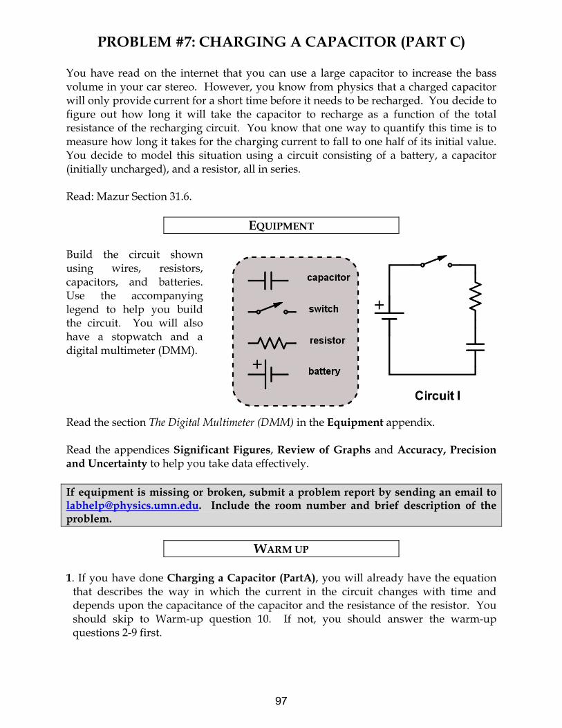
PROBLEM #7: CHARGING A CAPACITOR (PART C)
You have read on the internet that you can use a large capacitor to increase the bass volume in your car stereo. However, you know from physics that a charged capacitor will only provide current for a short time before it needs to be recharged. You decide to figure out how long it will take the capacitor to recharge as a function of the total resistance of the recharging circuit. You know that one way to quantify this time is to measure how long it takes for the charging current to fall to one half of its initial value. You decide to model this situation using a circuit consisting of a battery, a capacitor (initially uncharged), and a resistor, all in series. Read: Mazur Section 31.6.
EQUIPMENT Build the circuit shown using wires, resistors, capacitors, and batteries. Use the accompanying legend to help you build the circuit. You will also have a stopwatch and a digital multimeter (DMM).
Read the section The Digital Multimeter (DMM) in the Equipment appendix. Read the appendices Significant Figures, Review of Graphs and Accuracy, Precision and Uncertainty to help you take data effectively. If equipment is missing or broken, submit a problem report by sending an email to [email protected]. Include the room number and brief description of the problem.
WARM UP 1. If you have done Charging a Capacitor (PartA), you will already have the equation
that describes the way in which the current in the circuit changes with time and depends upon the capacitance of the capacitor and the resistance of the resistor. You should skip to Warm-up question 10. If not, you should answer the warm-up questions 2-9 first.
97

CHARGING A CAPACITOR (PART C)
2. Draw a circuit diagram, similar to the one shown above. Decide on the properties of each of the elements of the circuit that are relevant to the problem, and label them on your diagram. Label the potential difference across each of the elements of the circuit. Label the current in the circuit and the charge on the capacitor.
3. Use energy conservation to write an equation relating the potential differences across
all elements of the circuit. Write an equation relating the potential difference across the capacitor plates and the charge stored on its plates. What is the relationship between the current through the resistor and the voltage across it? Are these three equations always true, or only for specific times?
4. Describe qualitatively how each quantity labeled on your diagram changes with time.
What is the voltage across each element of the circuit (a) at the instant the circuit is closed; (b) when the capacitor is fully charged? What is the current in the circuit at these two times? What is the charge on the capacitor plates at these two times?
5. From the equations you constructed above, determine an equation relating the
voltage of the battery, the capacitance of the capacitor, the resistance of the resistor, the current through the circuit, and the charge stored on the capacitor plates.
6. Write an equation relating the rate of charge accumulation on the capacitor plates to
the current through the circuit. 7. Use the equations you have written to get a single equation that relates the current
and the rate of change of current to the known properties of each circuit element. To do this, you may find it helpful to differentiate one of your equations.
8. Solve the equation from step 6 by using one of the following techniques: (a) Guess the
current as a function of time, which satisfies the equation, and check it by substituting your current function into your equation; (b) Get all the terms involving current on one side of the equation and time on the other side and solve. Solving the equation may require an integral.
9. Complete your solution by determining any arbitrary constants in your solution,
using the initial value of the current you obtained in question 3. 10. Using your equation for the current, find the time it takes for the current to fall to
half its initial value. Sketch a graph of this time against the resistance of the resistor.
98

CHARGING A CAPACITOR (PART C)
PREDICTION
For a circuit consisting of a battery, a capacitor (initially uncharged), and a resistor, all in series, how does the time it takes for the current in the circuit to fall to half its initial value depend on the resistance of the resistor? Use your calculation to graph the time it takes for the current to fall to half its initial value against the resistance of the resistor.
EXPLORATION
WARNING: A charged capacitor can discharge quickly producing a painful spark. Do not handle the capacitors by their electrical terminals or connected wires by their metal ends. Always discharge a capacitor when you are finished using it. Before you build the circuit, examine each element of it. How do you know if the battery is "good"? Is the capacitor charged? Carefully connect the two terminals of the capacitor to ensure it is uncharged. How can you determine the resistance of the resistor? Is there a way to confirm it? If you have completed Charging a Capacitor (PartA) or (PartB), review your exploration notes from your lab journal. Note: Make sure the + terminal of the battery is connected to the + terminal of the capacitor! These capacitors are only designed to charge one way. If you connect the capacitors up the wrong way, the capacitance will change in an unpredictable manner. Construct Circuit I, including a DMM in the circuit to measure the current. Check that the polarity of the capacitor’s connection is correct and begin your experiment. Close the circuit and observe how long it takes for the current in the circuit to halve. How does changing the capacitance of the capacitor or the resistance of the resistor affect this time? Choose a capacitor and a range of resistances that allow you to effectively construct a graph and test your prediction. Complete your measurement plan.
MEASUREMENT Measure the time taken for the current in the circuit to halve in value for different resistances in the circuit. Be sure to make at least two measurements for each resistor.
99

CHARGING A CAPACITOR (PART C)
ANALYSIS Construct a graph of the measured times it takes the current to halve against resistance, using your experimental data.
CONCLUSION Compare your prediction graph with your graph showing your data. Explain any differences. How does the time taken for the current in the circuit to halve in value depend upon the resistance of the charging circuit? Does this time depend upon the voltage of the battery? If yes, then how? What are possible sources of systematic uncertainty in this experiment? How do contributions to the systematic uncertainty from the equipment imperfections and from human error compare? Provide detailed explanations. If needed, review the appendix material on uncertainty.
100
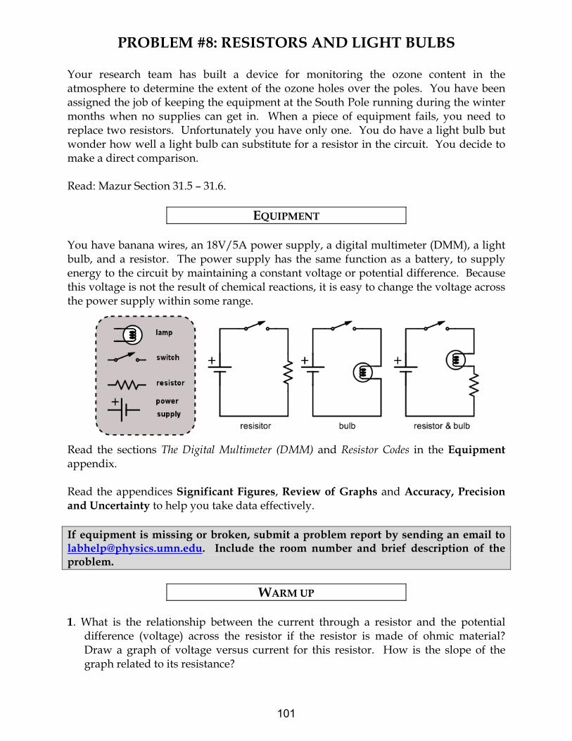
PROBLEM #8: RESISTORS AND LIGHT BULBS
Your research team has built a device for monitoring the ozone content in the atmosphere to determine the extent of the ozone holes over the poles. You have been assigned the job of keeping the equipment at the South Pole running during the winter months when no supplies can get in. When a piece of equipment fails, you need to replace two resistors. Unfortunately you have only one. You do have a light bulb but wonder how well a light bulb can substitute for a resistor in the circuit. You decide to make a direct comparison. Read: Mazur Section 31.5 – 31.6.
EQUIPMENT You have banana wires, an 18V/5A power supply, a digital multimeter (DMM), a light bulb, and a resistor. The power supply has the same function as a battery, to supply energy to the circuit by maintaining a constant voltage or potential difference. Because this voltage is not the result of chemical reactions, it is easy to change the voltage across the power supply within some range.
Read the sections The Digital Multimeter (DMM) and Resistor Codes in the Equipment appendix. Read the appendices Significant Figures, Review of Graphs and Accuracy, Precision and Uncertainty to help you take data effectively. If equipment is missing or broken, submit a problem report by sending an email to [email protected]. Include the room number and brief description of the problem.
WARM UP 1. What is the relationship between the current through a resistor and the potential
difference (voltage) across the resistor if the resistor is made of ohmic material? Draw a graph of voltage versus current for this resistor. How is the slope of the graph related to its resistance?
101

RESISTORS AND LIGHT BULBS
2. As more current goes through a light bulb, it gets brighter. As it gets brighter, it gets
hotter. Do you expect the increasing temperature to affect the resistance of the bulb? If so, how?
3. Sketch a qualitative graph of voltage across a light bulb versus current through the
light bulb.
PREDICTION Restate what elements of electric circuits (and by what criteria/parameters) you are to compare in this problem. Use your experience to draw a graph of voltage versus current for (a) a standard resistor, and (b) a light bulb. Explain your reasoning, including physical assumptions you have made.
EXPLORATION
WARNING: You will be working with a power supply that can generate large electric voltages. Improper use can cause painful burns. To avoid danger, the power must be turned OFF and you must wait at least one minute before any wires are disconnected from or connected to the power supply. Never grasp a wire by its metal end.
Sketch the circuit you will build to check your prediction. Can you test both the light bulb and the resistor at the same time? Is this a good idea? If necessary, read about how to use the DMM in the Equipment appendix. Pay special attention to the connections and settings that are used to measure voltages and currents, and why the DMM should be connected in the circuit differently for voltage and current measurements. Do you know why we should connect them in these ways?
MEASUREMENT There are three methods for determining the electrical resistance of a resistor. 1. Use the chart provided in the appendix to determine the resistance of your resistor
based on its color code. What is the uncertainty in this value? 2. Use the DMM set to ohms to measure the resistance of the resistor. What is the
uncertainty in this value? Why is this procedure not helpful with a light bulb?
102

RESISTORS AND LIGHT BULBS
3. Use your power supply, DMM, and resistor to determine the voltage across the resistor and measure the current through the resistor for several different voltages. What is the uncertainty in the value of the resistance obtained by this method?
ANALYSIS
Make a graph of voltage versus current for your resistor and light bulb. How do the values of the resistance compare for the different methods used?
CONCLUSION Are the color-coded resistor and light bulb both ohmic resistors? If so, what are their resistances? Did your prediction match your results? If not, can you use the bulb over some limited range of voltages? What range? Explain your reasoning. What are possible sources of systematic uncertainty? (If you need help determining uncertainty see the appendices Significant Figures and Accuracy, Precision and Uncertainty) Does the equipment contribute any? Do you? Be specific in explaining how and why.
103

RESISTORS AND LIGHT BULBS
104
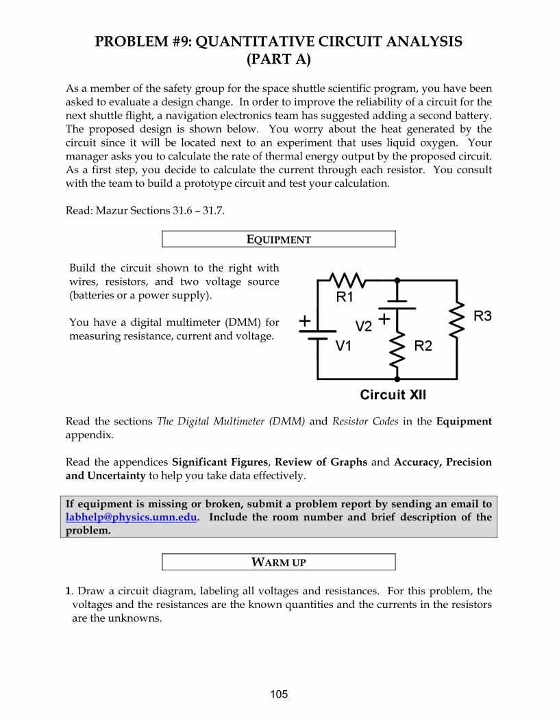
PROBLEM #9: QUANTITATIVE CIRCUIT ANALYSIS (PART A)
As a member of the safety group for the space shuttle scientific program, you have been asked to evaluate a design change. In order to improve the reliability of a circuit for the next shuttle flight, a navigation electronics team has suggested adding a second battery. The proposed design is shown below. You worry about the heat generated by the circuit since it will be located next to an experiment that uses liquid oxygen. Your manager asks you to calculate the rate of thermal energy output by the proposed circuit. As a first step, you decide to calculate the current through each resistor. You consult with the team to build a prototype circuit and test your calculation. Read: Mazur Sections 31.6 – 31.7.
EQUIPMENT Build the circuit shown to the right with wires, resistors, and two voltage source (batteries or a power supply). You have a digital multimeter (DMM) for measuring resistance, current and voltage.
Read the sections The Digital Multimeter (DMM) and Resistor Codes in the Equipment appendix. Read the appendices Significant Figures, Review of Graphs and Accuracy, Precision and Uncertainty to help you take data effectively. If equipment is missing or broken, submit a problem report by sending an email to [email protected]. Include the room number and brief description of the problem.
WARM UP 1. Draw a circuit diagram, labeling all voltages and resistances. For this problem, the
voltages and the resistances are the known quantities and the currents in the resistors are the unknowns.
105

QUANTITATIVE CIRCUIT ANALYSIS (PART A)
2. Assign a separate current for each leg of the circuit, indicating each current on the diagram. Identify the number of circuit paths (loops) and label them on the diagram.
3. Apply conservation of current to each point in the circuit at which wires come
together (a junction). Use conservation of energy to get the sum of the potential differences across all of the elements in each loop, ensuring your signs are correct. Does the potential difference increase or decrease across each circuit element, in the direction you have chosen to traverse the loop? Use Ohm's law to get the potential difference across each resistor. Check that the number of equations you wrote above matches the number of unknowns.
4. Complete the calculations and write your solution. Simplify your equations as much
as possible, but be warned that your final solutions may look quite complicated.
PREDICTION To predict currents through resistors in the circuit under study, you will need to use Kirchoff’s laws. The goal is to derive theoretical formulas for the currents. Once you have the formulas, you can plug in the parameters of your circuit, such as voltages of the batteries and resistances of resistors, and calculate the currents. These (predicted) values will be compared with the currents measured in the experiment.
EXPLORATION If necessary, read about how to use the DMM in the Equipment appendix. Pay special attention to the connections and settings that are used to measure voltages and currents, and why the DMM should be connected in the circuit differently for voltage and current measurements. Do you know why we should connect them in these ways? Build Circuit XII. How can you tell if there is current flowing through the circuit? What happens to the current at each junction? What is the resistance of each resistor? What is the potential difference provided by each of the batteries? What is the potential difference across each resistor? Use the DMM to check your answers to each of these questions. Complete your measurement plan.
106
QUANTITATIVE CIRCUIT ANALYSIS (PART A)
MEASUREMENT
Measure the resistance of the resistors, the current flowing through each resistor and the potential difference provided by each battery in the circuit. So that you can check your measurements, measure the potential difference across each resistor.
ANALYSIS Calculate the current through each resistor from your prediction equations, using your measured values of the resistance of each resistor and voltage of each battery. Compare those results to the measured values of each current.
CONCLUSION Did your measured and predicted values of the currents through the resistors agree? If not, explain the discrepancy. As a check for the consistency of your measurements, calculate the potential difference across each resistor using the currents that you measured. Compare these values with the potential difference across each resistor that you measured with the DMM.
107

QUANTITATIVE CIRCUIT ANALYSIS (PART A)
108
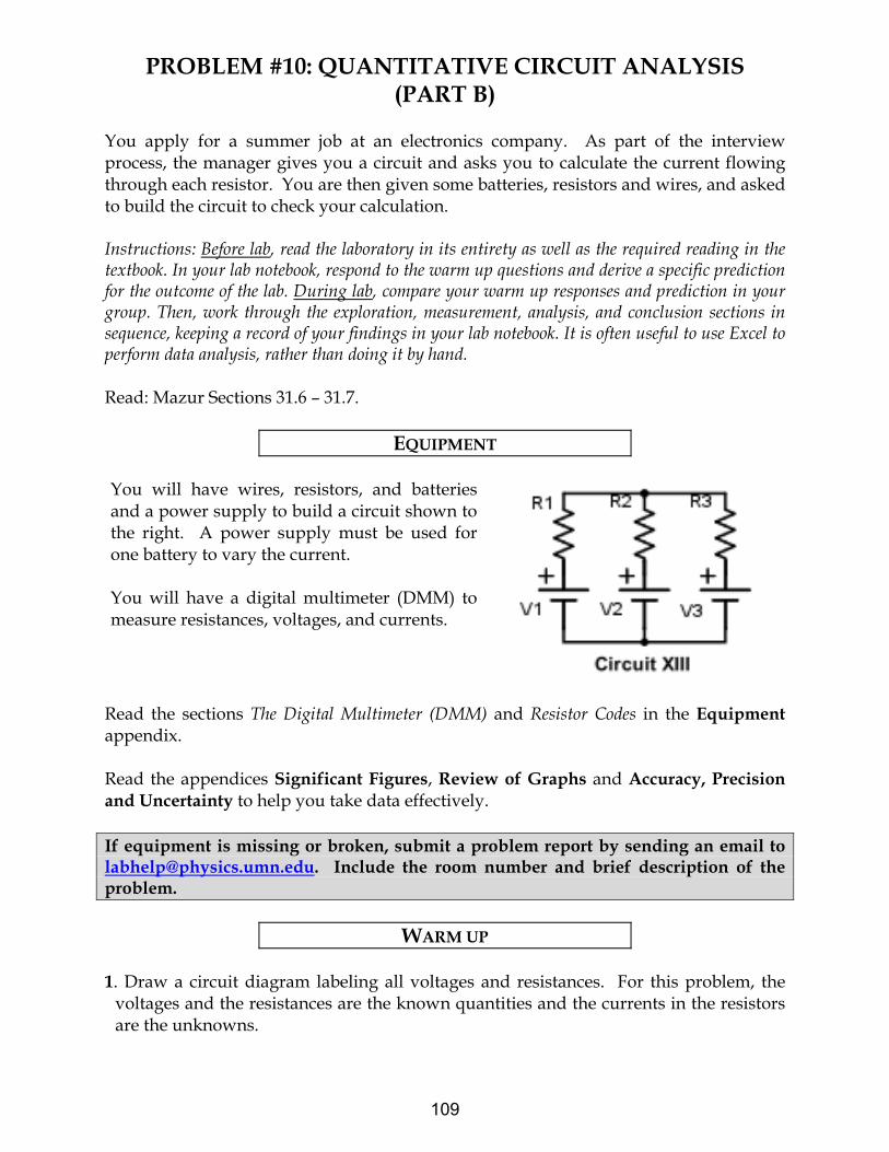
PROBLEM #10: QUANTITATIVE CIRCUIT ANALYSIS (PART B)
You apply for a summer job at an electronics company. As part of the interview process, the manager gives you a circuit and asks you to calculate the current flowing through each resistor. You are then given some batteries, resistors and wires, and asked to build the circuit to check your calculation. Instructions: Before lab, read the laboratory in its entirety as well as the required reading in the textbook. In your lab notebook, respond to the warm up questions and derive a specific prediction for the outcome of the lab. During lab, compare your warm up responses and prediction in your group. Then, work through the exploration, measurement, analysis, and conclusion sections in sequence, keeping a record of your findings in your lab notebook. It is often useful to use Excel to perform data analysis, rather than doing it by hand. Read: Mazur Sections 31.6 – 31.7.
EQUIPMENT You will have wires, resistors, and batteries and a power supply to build a circuit shown to the right. A power supply must be used for one battery to vary the current. You will have a digital multimeter (DMM) to measure resistances, voltages, and currents.
Read the sections The Digital Multimeter (DMM) and Resistor Codes in the Equipment appendix. Read the appendices Significant Figures, Review of Graphs and Accuracy, Precision and Uncertainty to help you take data effectively. If equipment is missing or broken, submit a problem report by sending an email to [email protected]. Include the room number and brief description of the problem.
WARM UP 1. Draw a circuit diagram labeling all voltages and resistances. For this problem, the
voltages and the resistances are the known quantities and the currents in the resistors are the unknowns.
109
QUANTITATIVE CIRCUIT ANALYSIS (PART B)
2. Assign a separate current for each leg of the circuit, indicating each current on the
diagram. Identify the number of circuit paths (loops) and label them on the diagram. 3. Apply conservation of current to each point in the circuit at which wires come
together (a junction). Use conservation of energy to get the sum of the potential differences across all of the elements in each loop, ensuring your signs are correct. Does the potential difference increase or decrease across each circuit element, in the direction you have chosen to traverse the loop? Use Ohm's law to get the potential difference across each resistor.
Check that the number of linear equations that you have now matches the number of unknowns.
4. Complete the calculations and write your solution. Simplify your equations as much as possible, but be warned that your final solutions may look quite complicated.
PREDICTION
Derive formulas to calculate the current through each of resistors in Circuit XIII as a function of voltages of the batteries and resistances involved in the circuit.
EXPLORATION If necessary, read about how to use the DMM in the appendix. Pay special attention to the connections and settings that are used to measure voltages and currents, and why the DMM should be connected in the circuit differently for voltage and current measurements. Do you know why we should connect them in these ways? Build Circuit XIII. How can you tell if there is current flowing through the circuit? What happens to the current at each junction? What is the resistance of each resistor? What is the potential difference provided by each of the batteries? What is the potential difference across each resistor? Use the DMM to check your answers to each of these questions. Complete your measurement plan.
MEASUREMENT Measure the resistance of each of the three resistors, as well as the currents flowing through each of them. Measure the potential difference provided by each battery. So
110

QUANTITATIVE CIRCUIT ANALYSIS (PART B)
that you can check your measurements, measure the potential difference across each resistor.
ANALYSIS Calculate the current through each resistor from your prediction equations, using your measured values of the resistance of each resistor and voltage of each battery. Compare those results to the measured values of each current.
CONCLUSION Did your measured and predicted values of the currents through the resistors agree? If not, explain the discrepancy. As a check for the consistency of your measurements, calculate the potential difference across each resistor using the currents that you measured. Compare these values with the potential difference across each resistor that you measured with the DMM.
111

QUANTITATIVE CIRCUIT ANALYSIS (PART B)
112
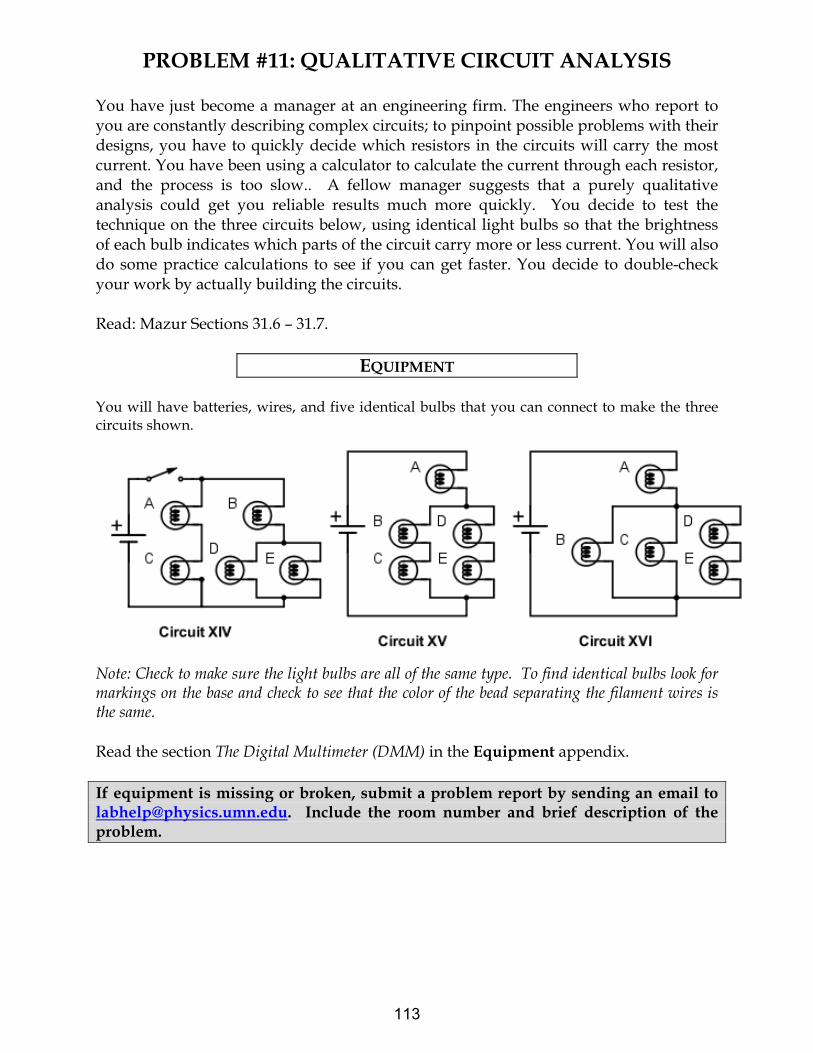
PROBLEM #11: QUALITATIVE CIRCUIT ANALYSIS
You have just become a manager at an engineering firm. The engineers who report to you are constantly describing complex circuits; to pinpoint possible problems with their designs, you have to quickly decide which resistors in the circuits will carry the most current. You have been using a calculator to calculate the current through each resistor, and the process is too slow.. A fellow manager suggests that a purely qualitative analysis could get you reliable results much more quickly. You decide to test the technique on the three circuits below, using identical light bulbs so that the brightness of each bulb indicates which parts of the circuit carry more or less current. You will also do some practice calculations to see if you can get faster. You decide to double-check your work by actually building the circuits. Read: Mazur Sections 31.6 – 31.7.
EQUIPMENT You will have batteries, wires, and five identical bulbs that you can connect to make the three circuits shown.
Note: Check to make sure the light bulbs are all of the same type. To find identical bulbs look for markings on the base and check to see that the color of the bead separating the filament wires is the same. Read the section The Digital Multimeter (DMM) in the Equipment appendix. If equipment is missing or broken, submit a problem report by sending an email to [email protected]. Include the room number and brief description of the problem.
113

QUALITATIVE CIRCUIT ANALYSIS
PREDICTIONS
You will need to use both qualitative rules and formulas from your text book to make predictions about the brightness of the light bulbs in the circuits under study. The following rules are nothing but consequences of conservation of charge, conservation of energy, and Ohm's law in electric circuits. 1. a) Resistors in series all have the same current flowing through them.
b) Resistances in series add. c) The current through a path across a fixed potential difference decreases as the total resistance of the path increases.
2. a) Current divides at a junction. b) The current through each path across the same potential difference depends on the resistance of the path – the larger the resistance, the smaller the current. c) Paths of equal resistance will have the same current.
3. a) Resistors in parallel offer less total resistance than the smallest resistance in the configuration.
b) Parallel branches connected directly across a battery are independent – each set of parallel branches has the same potential difference as if it were the only connection to the battery.
The above rules will help you predict how the bulbs within each circuit should compare in brightness. Include in each prediction, which rule(s) you used answering the question. Circuit XIV How will the brightness of bulb A compare with the brightness of bulb B? How will the brightness of bulb B compare with the brightness of bulb D? How will the brightness of bulb C compare with the brightness of bulb D? Circuit XV How will the brightness of bulb A compare with the brightness of bulb B? How will the brightness of bulb B compare with the brightness of bulb C? How will the brightness of bulb B compare with the brightness of bulb D? Circuit XVI How will the brightness of bulb A compare with the brightness of bulb B? How will the brightness of bulb B compare with the brightness of bulb C? How will the brightness of bulb B compare with the brightness of bulb D?
114

QUALITATIVE CIRCUIT ANALYSIS
Now, try to rank the circuits by the brightness of bulb A. First decide which quantity the brightness of a bulb depends on. Then construct an equation for this quantity in terms of two variables – the resistance of each bulb, say R, (remember that all the bulbs are identical) and the voltage of each battery, say V (same in each of the three circuits). Begin by finding equivalent resistances of certain parts of the circuits. Gradually simplify each circuit applying appropriate equations to pairs of bulbs in series or in parallel up to the point when you can use qualitative considerations to rank the circuits by the current through bulb A or by the potential difference across this bulb.
EXPLORATION Set up each circuit and observe the brightness of the bulbs. How can you test whether minor differences you observe are due to manufacturing irregularities in “identical” bulbs?
MEASUREMENT Coordinate with other groups to compare the brightness of bulb A in each of the three circuits. If necessary, use a DMM to measure the current through bulb A in each of the three circuits. When using the DMM, pay special attention to the connections and settings that are used to measure voltages and currents and why the DMM should be connected in the circuit differently for voltage and current measurements. Do you know why we should connect them in these ways?
CONCLUSION Qualitative circuit analysis is very useful for quickly checking the results of the algebra that come from quantitative circuit analysis. It is a great way to catch mistakes before you fry expensive circuits. Explain any differences between your predictions and your observations. Each qualitative rule is the result of applying conservation of energy (Kirchhoff's loop rule), conservation of charge (Kirchhoff's junction rule), and Ohm’s law to different circuit configurations. . To summarize the material learned, for each qualitative rule, write the corresponding equation(s).
115

QUALITATIVE CIRCUIT ANALYSIS
116

CHECK YOUR UNDERSTANDING LAB 4: CIRCUITS
1. What would happen to the brightness of bulb A in the circuit below if more bulbs were added
parallel to bulbs B and C?
In household circuits, a fuse or circuit breaker is in the position occupied by bulb A, why?
2. Rank Circuits I through IV from the largest current at point 1 to the smallest current at point 1.
Explain your reasoning.
3. Predict what will happen to the brightness of bulbs A, B, C and D if bulb E were removed from its
socket. Explain your reasoning.
117

CHECK YOUR UNDERSTANDING LAB 4: CIRCUITS
4. For the circuit below, determine the current in each resistor.
5. For the circuit below, determine the value for R such that the current I3 is 0.1A with the indicated
direction.
What is the value for R that will give a current I3 = 0.1 A, but in the opposite direction to what is
shown?
+-
+- 12 V24 V
8
6
3624
12
+- 3 V R
20
+-
6 V
5
I3
118

Physics Lab Report Rubric
Name: ID#:Course, Lab Sequence, and Problem Number:Date Performed:Lab Partners’ Names:
Possible Earned
Warm-Up Questions
Possible Earned
Laboratory Notebook
Earns No Points Earns Full Points Possible EarnedArgument
• no clear argument• logic does not flow• gaps in content• leaves reader with questions
• complete, cogent, flowing argument• context, execution, analysis, conclu-
sion all present• leaves reader satisfied
Technical Style
• vocabulary, syntax, etc. inappropri-ate for scientific writing
• necessary nonverbal media absent orpoorly constructed
• subjective, fanciful, or appealing toemotions
• jarringly inconsistent
• language is appropriate• nonverbal media present where ap-
propriate, well constructed, well in-corporated
• objective, indicative, logical style• consistent style• division into sections is helpful
Use of Physics
• predictions with no or with unphysi-cal justification
• experiment physically unjustified• experiment tests wrong phenomenon• theory absent from consideration of
premise, predictions, and results
• predictions are justified with physicaltheory
• experiment is physically sound andactually tests phenomenon in ques-tion
• results interpreted with theory toclear, appropriate conclusion
Quantitativeness
• statements are vague or arbitrary• analysis is inappropriately qualitative• error analysis not used to evaluate
prediction or find result• numbers, equations, units, uncertain-
ties missing or inappropriate
• consistently quantitative• equations, numbers with units, uncer-
tainties throughout• prediction confirmed or denied, result
found by error analysis• results, conclusions based on data
Total
119

120

LAB 5: MAGNETIC FIELDS AND FORCES
Magnetism plays a large part in our modern world 's technology. Magnets are used today to
image parts of the body, to explore the mysteries of the human brain, and to store analog and
d igital data. Magnetism also allows us to explore the structure of th e Universe, the atomic
structure of materials, and the quark structure of elementary particles.
In this set of laboratory problems, you will map magnetic fields from d ifferent sources and use
the magnetic force to deflect electrons. The magnetic interaction can best be described using
the concept of a field . For this reason, your experiences exploring the electric field concept in
the first lab are also applicable in this lab. There are similar activities in both labs so you can
experience the universality of the field concept. Although they are related , the magnetic force
is not the same as the electric force. You should watch for the d ifferences as you go through
the problems in this lab.
OBJECTIVES:
After successfully completing this laboratory, you should be able to:
• Explain the d ifferences and similarities between magnetic fields and electric fields.
• Describe magnetic fields near sources, such as permanent “bar” magnets, straight
current-carrying wires, and coils of wire.
• Calculate the magnetic force on a charged particle moving in a uniform magnetic
field and describe its motion.
PREPARATION:
Read Mazur Chapters 27 and 28. Review your notes from the first lab (Electric Fields and
Forces).
Before coming to lab you should be able to:
Add fields using vector properties.
Use the vector cross product.
Calculate the motion of a particle with a constant acceleration.
Calculate the motion of a particle with an acceleration of constant magnitude
perpendicular to its velocity.
Write down the magnetic force on an object in terms of its charge, velocity, and the
magnetic field through which it is passing.
121

LAB 5: MAGNETIC FIELDS AND FORCES
122

PROBLEM #1: PERMANENT MAGNETS
You have a job working at a company that designs magnetic resonance imaging (MRI) machines. The ability to get a clear image of the inside of the body depends on knowing precisely the correct magnetic field at that position. In a new model of the machine, the magnetic fields are produced by configurations of permanent magnets. You need to know the map of the magnetic field from each magnet and how to combine magnets to change the magnetic field at any point. You decide to determine the form of the magnetic field for various combinations of bar magnets, and to draw vector diagrams (field maps) for each combination. Instructions: Before lab, read the laboratory in its entirety as well as the required reading in the textbook. In your lab notebook, respond to the warm up questions and derive a specific prediction for the outcome of the lab. During lab, compare your warm up responses and prediction in your group. Then, work through the exploration, measurement, analysis, and conclusion sections in sequence, keeping a record of your findings in your lab notebook. It is often useful to use Excel to perform data analysis, rather than doing it by hand. Read: Mazur Sections 27.1 - 27.2.
EQUIPMENT You will have two permanent magnets, a magnetizer (if needed) and a clear plate filled with a viscous liquid and particles of taconite. When a magnet is placed on top of one of these plates, the Taconite pieces align themselves with the magnetic field. You will also have a compass. The magnet configurations you need to consider are as follows:
N
S
N
S
N
S N
SN
S
Figure I
Figure IV Figure V
Figure II
Figure III
N
S
Figure VI
Read the section Magnetizing a Bar Magnet in the Equipment appendix if you need to re-magnetize your magnets. If equipment is missing or broken, submit a problem report by sending an email to [email protected]. Include the room number and brief description of the problem.
123

PERMANENT MAGNETS
WARM UP
1. Make a sketch of all the magnets in each figure. Be sure to label the poles of the
magnets.
2. Choose a point near the pole of a magnet. At that point draw a vector representing the magnetic field. The length of the vector should give an indication of the strength of the field. Keep in mind that:
The field can have only one value and direction at any point.
The direction of the magnetic field points away from a North pole, and towards a South pole.
The field at a point is the vector sum of the fields from all sources.
3. Move a short distance away in the direction of the vector and choose another point. At that point draw another magnetic field vector. Continue this process until you reach another magnetic pole. Choose another point near a pole and start the process again. Continue until you can see the pattern of the magnetic field for all parts of the configuration.
PREDICTION
Sketch a map of the magnetic field for each magnet configuration in the figures in the equipment section. Assume that the different magnet configurations in each figure do not interact with the magnets in the other figures.
EXPLORATION
WARNING: The viscous liquid (glycerin) in the Taconite plate may cause skin irritation. If a plate is leaking, please notify your lab instructor immediately.
WARNING: Strong magnetic fields can affect pacemakers, ICDs and other implanted medical devices. Many of these devices are made with a feature that deactivates it with a magnetic field. Therefore, care must be taken to keep medical devices minimally 1’ away from any strong magnetic field.
Check to make sure your Taconite plate is not leaking. Gently shake the plate until the Taconite is distributed uniformly (the transparent bar inside the plate will help redistribute the flecks when moved).
124

PERMANENT MAGNETS
Properties of magnets can change with handling. Check the poles of the magnet with your compass. Inform your lab instructor if the magnet does not behave as you would expect, a magnetizer can be used to correct the polarity and intensity if necessary. Place a permanent magnet on the Taconite plate. If the flecks are difficult to see, put a piece of white paper behind the plate. How long must you wait to see the effect of the magnetic field? Is it what you expected? Try some small vibrations of the Taconite plate. How does the pattern in the Taconite relate to the direction that a compass needle points when it is directly on top of the Taconite sheet? Try different configurations of magnets and determine how to get the clearest pattern in the Taconite. What can you do to show that the poles of a magnet are not electric charges? Try it.
MEASUREMENT AND ANALYSIS Lay one bar magnet on the Taconite plate. In your journal, draw the pattern of the magnetic field produced. Repeat for each figure in the predictions.
CONCLUSION How did your predictions of the shape of the magnetic field for each configuration of magnets compare with your results? What influence does the field have on the Taconite filings? Does the field cause a net force? Does the field cause a net torque? If so, in what direction?
125

PERMANENT MAGNETS
126

PROBLEM #2: CURRENT CARRYING WIRE
Your friend's parents, who live on a dairy farm, have high-voltage power lines across their property. They are concerned about the effect the magnetic field from the power lines might have on the health of their dairy cows grazing nearby. They bought a device to measure the magnetic field. The instructions for the device state that it must be oriented perpendicular to the magnetic field. To measure the magnetic field correctly, they need to know its direction at points near a current carrying wire. They know you have taken physics, so they ask you for help. First, you decide to check a simulation of the magnetic field of a current carrying wire. Next, to confirm your prediction and simulation, you decide to use a compass along with a current carrying wire. You decide to investigate both a straight wire and a loop of wire. Instructions: Before lab, read the laboratory in its entirety as well as the required reading in the textbook. In your lab notebook, respond to the warm up questions and derive a specific prediction for the outcome of the lab. During lab, compare your warm up responses and prediction in your group. Then, work through the exploration, measurement, analysis, and conclusion sections in sequence, keeping a record of your findings in your lab notebook. It is often useful to use Excel to perform data analysis, rather than doing it by hand. Read:Mazur Sections 27.3 and 28.2.
EQUIPMENT You will have a Hall probe and interface, a magnetic compass, banana cables, a meter stick, an 18volt/5amp power supply and the Magnetism 3D simulation. Make sure to use the correct power supply – do not use the Cenco CRT power supplies, they are not designed to be used in this manner! Read the section The Magnetic Field Sensor (Hall Probe) in the Equipment appendix. Read the section Measuring Constant Magnetic Field in the Software appendix. If equipment is missing or broken, submit a problem report by sending an email to [email protected]. Include the room number and brief description of the problem.
PREDICTIONS Sketch your best guess of the map of the magnetic field near a current carrying wire when the wire is (a) stretched straight, and (b) formed into a loop.
127

CURRENT CARRYING WIRE
EXPLORATION
Start the Magnetism 3D simulation. To study magnetic fields of current carrying wires, you will want to choose Add Unlimited Vertical Wire or Add Vertical Wire Loop from the Add menu. Once you have added an element to the workspace, you should select Draw Magnetic Field (B) Lines from the Field menu. Now you can scroll the cursor around the workspace and the simulation will display a vector and show the position and magnitude of the field along the bottom of the workspace. You can click the mouse with the cursor in a specific location and an infinite field line will appear. Once you have a clear picture of what the direction of the field is, you can create a pdf file using the Print command under File. You might also find it useful to play around with different sizes of current to note any changes. Once you are finished with Magnetism 3D, it is time to move to the physical apparatus. Keep in mind that a compass needle, because it is a small magnet, aligns itself parallel to the local magnet field. Attach enough wires together to give a total length of at least half a meter. Is there any evidence of a magnetic field from a non-current carrying wire? To check this, stretch the wire vertically and move your compass around the wire. Does the compass always point in the same direction?
WARNING: You will be working with a power supply that can generate large electric voltages. Improper use can cause painful burns. To avoid danger, the power should be turned OFF and you should WAIT at least one minute before any wires are disconnected from or connected to the power supply. NEVER GRASP A WIRE BY ITS METAL ENDS!
WARNING: Strong magnetic fields can affect pacemakers, ICDs and other implanted medical devices. Many of these devices are made with a feature that deactivates it with a magnetic field. Therefore, care must be taken to keep medical devices minimally 1’ away from any strong magnetic field.
Connect the wire to the power supply and turn the power supply on (do not use the Cenco CRT power source). Stretch the wire vertically and move your compass around the wire. Start where you expect the magnetic field to be largest. Is there any evidence of a magnetic field from a current carrying wire? Watch the compass as you turn the current on and off. Does the compass always point in the same direction? How far from the wire can the compass be and still show a deflection? Develop a measurement plan.
128

CURRENT CARRYING WIRE
Now make a single loop in the wire through which you can easily move the compass. Move the compass around the loop. In which direction is the compass pointing? How far away from the loop can you see a deflection? Is this distance larger along the axis of the loop or somewhere else? Set up your Hall probe as explained in the Equipment and Software appendices. Before you push any buttons on the computer, locate the magnetic field strength window. You will notice that even when the probe is held away from obvious sources of magnetic fields, such as your bar magnets, you see a non-zero reading. From its behavior determine if this is caused by a real magnetic field or is an electronics artifact or both? If you notice an ambient field, can you determine its cause? Go through the Hall probe calibration procedure outlined in the Magnetlab Guide Box in the upper right corner of the application. Does the Hall probe ever read a zero field? Hold the Hall probe next to the wire; how can you use the information from your compass to decide how to orient the probe? Read the value displayed by the MagnetLab program. What will happen when you move the probe further from the wire? Will you have to change the orientation of the probe? How will you measure the distance of the probe from the wire?
MEASUREMENT Use your measurement plan to create a map of the magnetic field around the stretched wire and the looped wire. Include the magnitude and direction of the magnetic field for each distance.
ANALYSIS The direction of the magnetic field at a point near a current-carrying wire can be found by using the "right-hand rule" that is described in your text. How does the "right-hand rule" compare to your measurements?
CONCLUSION How did your predictions of the map of the magnetic field near current-carrying wires compare with both physical and simulated results? How do they compare with the "right-hand rule"?
129

CURRENT CARRYING WIRE
130

PROBLEM #3: MEASURING THE MAGNETIC FIELD OF PERMANENT MAGENTS
Your team is designing a probe to investigate space near Jupiter. One device uses strong permanent magnets to track the motion of charged particles through Jupiter’s magnetic field. You worry that their magnetic fields could damage computers on the probe. To estimate how close a magnet can be to a computer without causing damage, you have been asked to determine the magnitude of the field near the magnet. No isolated magnetic monopoles have ever been discovered (a difference between magnetism and electricity) but you wonder how accurately one could mathematically model the field of a bar magnet as the vector sum of fields produced by monopoles located near each end of the magnet. With this model, you calculate how the magnetic field would vary with distance along each symmetry axis of a bar magnet. You assume that a magnetic monopole would produce a magnetic field similar to the electric field produced by a point charge. To test your model, you decide to measure the magnetic field near a bar magnet with a Hall probe. Instructions: Before lab, read the laboratory in its entirety as well as the required reading in the textbook. In your lab notebook, respond to the warm up questions and derive a specific prediction for the outcome of the lab. During lab, compare your warm up responses and prediction in your group. Then, work through the exploration, measurement, analysis, and conclusion sections in sequence, keeping a record of your findings in your lab notebook. It is often useful to use Excel to perform data analysis, rather than doing it by hand. Review your notes from the earlier problem: Electric Field from a Dipole
EQUIPMENT You will have a bar magnet, a meter stick, a Hall probe and a computer data acquisition system. You will also have a taconite plate and a compass. Read the section The Magnetic Field Sensor (Hall Probe) in the Equipment appendix. Read the section Measuring Constant Magnetic Field in the Software appendix. If equipment is missing or broken, submit a problem report by sending an email to [email protected]. Include the room number and brief description of the problem.
WARM UP 1. Draw a bar magnet as a magnetic dipole consisting of two magnetic monopoles of
equal strength but opposite sign, separated by some distance. Label each monopole
131
MEASURING THE MAGNETIC FIELD OF PERMANENT MAGNETS
with its strength and sign, using the symbol “g” to represent the strength of the monopole. Label the distance. Choose a convenient coordinate system.
2. Select a point along one of the coordinate axes, outside the magnet, at which you will calculate the magnetic field. Determine the position of that point with respect to your coordinate system. Determine the distance of your point to each pole of the magnet, in terms of the position of your point with respect to your coordinate system.
3. Assume that the magnetic field from a magnetic monopole is analogous to the electric field from a point charge, i.e. the magnetic field is proportional to g/r2 where g is a measure of the strength of the monopole. (What are the dimensions of this “g”?) Determine the direction of the magnetic field from each pole at the point of interest.
4. Calculate the magnitude of each component of the magnetic field from each pole at the point of interest. Add the magnetic field (remember it is a vector) from each pole at that point to get the magnetic field at that point.
5. Graph your resulting equation for magnetic field strength along that axis as a function of position along the axis.
6. Repeat the above steps for the other axis.
PREDICTION Calculate the magnetic field strength as a function of distance along each axis of a bar magnet. Make a graph of this function for each axis. How do you expect these graphs to compare to similar graphs of the electric field along each axis of an electric dipole?
EXPLORATION
WARNING: Strong magnetic fields can affect pacemakers, ICDs and other implanted medical devices. Many of these devices are made with a feature that deactivates it with a magnetic field. Therefore, care must be taken to keep medical devices minimally 1’ away from any strong magnetic field.
Using either a taconite plate or compass, check that the magnetic field of the bar magnet appears to be a dipole. Start the MagnetLab program and follow the Hall probe calibration procedure outlined in the Software appendix. Instructions for using Magnetlab are also displayed in the Magnetlab Guide Box in the upper right corner of the application. Take one of the bar magnets and use the probe to check the variation of the magnetic field. Based on your previous determination of the magnetic field map, be sure to
132

MEASURING THE MAGNETIC FIELD OF PERMANENT MAGNETS
orient the Hall probe correctly. Where is the field the strongest? The weakest? How far away from the bar magnet can you still measure the field with the probe? Write down a measurement plan.
MEASUREMENT Based on your exploration, choose a scale for your graph of magnetic field strength against position that will include all of the points you will measure. Choose an axis of the bar magnet and take measurements of the magnetic field strength in a straight line along the axis of the magnet. Be sure that the field is always perpendicular to the probe. Make sure a point appears on the graph of magnetic field strength versus position every time you enter a data point. Use this graph to determine where you should take your next data point to map out the function in the most efficient manner. Repeat for each axis of the magnet.
ANALYSIS Compare the graph of your calculated magnetic field to that which you measured for each axis of symmetry of your bar magnet. Can you fit your prediction equation to your measurements by adjusting the constants?
CONCLUSION Along which axis of the bar magnet does the magnetic field fall off faster? Did your measured graph agree with your predicted graph? If not, why? State your results in the most general terms supported by your analysis. How would the shape of the graph of magnetic field strength versus distance for the magnetic dipole compare to the shape of the graph of electric field strength versus distance for an electric dipole? Is it reasonable to assume that the functional form of the magnetic field of a monopole is the same as that of an electric charge? Explain your reasoning.
133

MEASURING THE MAGNETIC FIELD OF PERMANENT MAGNETS
134

PROBLEM #4: THE MAGNETIC FIELD OF ONE COIL
You are working with a group researching new techniques to miniaturize the read-write head (the device in hard drives that reads and writes data to the disk). You suggest that a permanent magnet in the head could be replaced with a loop of wire to control the strength of the magnetic field. You read in your physics text that a coil of wire carrying a current gives the same magnetic field as a bar magnet: a magnetic dipole field. Your partners doubt that this is the case, so you decide to check it using a large coil of wire and a Hall probe, as well as a simulation. You decide to measure the strength of the magnetic field as a function of position along the central axis of the coil and compare it to the measurements you have for a bar magnet. As a qualitative check you also use the Hall probe to make a map of the magnetic field everywhere near the current carrying coil, and compare that to what the simulation predicts. Instructions: Before lab, read the laboratory in its entirety as well as the required reading in the textbook. In your lab notebook, respond to the warm up questions and derive a specific prediction for the outcome of the lab. During lab, compare your warm up responses and prediction in your group. Then, work through the exploration, measurement, analysis, and conclusion sections in sequence, keeping a record of your findings in your lab notebook. It is often useful to use Excel to perform data analysis, rather than doing it by hand. Review Measuring the Magnetic Field of Permanent Magnets
EQUIPMENT You have a coil of 200 turns of wire, an 18volt/5amp power supply, a compass, meterstick, digital multimeter (DMM), Hall probe and a computer data acquisition system. You will also have the Magnetism 3D application. Do not use the Cenco CRT power supply for this problem.
Power Supply
x
yDMM
Read the sections The Magnetic Field Sensor (Hall Probe) & The Digital Multimeter in the Equipment appendix. Read the section Measuring Constant Magnetic Field in the Software appendix. If equipment is missing or broken, submit a problem report by sending an email to [email protected]. Include the room number and brief description of the problem.
135

THE MAGNETIC FIELD OF ONE COIL
WARM UP
If you have done the problem Measuring the Magnetic Field of Permanent Magnets, review your lab journal for that problem. If not, answer the warm-up questions below to determine this. 1. Draw a bar magnet as a magnetic dipole consisting of two magnetic monopoles of
equal strength but opposite sign, separated by some distance. Label each monopole with its strength and sign. Label the distance. Choose a convenient coordinate system.
2. Select a point along one of the coordinate axes, outside the magnet, at which you will calculate the magnetic field. Determine the position of that point with respect to your coordinate system. Determine the distance of your point to each pole of the magnet, using your coordinate system.
3. Assume that the magnetic field from a magnetic monopole is analogous to the electric field from a point charge, i.e. the magnetic field is proportional to g/r^2 where g is a measure of the strength of the monopole. Determine the direction of the magnetic field from each pole at the point of interest.
4. Calculate the magnitude of the each component of the magnetic field from each pole at the point of interest. Add the magnetic field (remember it is a vector) from each pole at that point to get the magnetic field at that point.
5. Graph your resulting equation for the magnetic field strength along that axis as a function of position along the axis.
6. Repeat the above steps for the other axis. Draw the coil and label the current through it. Using the right hand rule, determine the direction of the magnetic field along the central axis of the coil. Using this information, which symmetry axis of a magnetic dipole corresponds to this central axis?
PREDICTION Compare the magnitude of the magnetic field as a function of distance along central axis of a coil of known radius and carrying a known electric current to that of a bar magnet. Also compare the field map of the current carrying coil with that of a bar magnet.
136

THE MAGNETIC FIELD OF ONE COIL
EXPLORATION
First, see what the Magnetism 3D simulation gives you. Start the application, and then select Add Solenoid, Vertical Wire Loop or Rectangular Magnet from the Add menu. To study magnetic fields of current carrying coil, you will likely want to select Add Solenoid, and then specify the properties of the coil desired. Don’t select over 25 loops per centimeter and de-select the option for an Iron Core when specifying the properties of the coil. Once an element has been added to the workspace, you should select Draw Magnetic Field (B) Lines from the Field menu. Now you can scroll the cursor around the workspace and the simulation will display a vector and show the position and magnitude of the field along the bottom of the workspace. You should pick points both inside and outside the coil for a complete map of the magnetic field. You can click the mouse with the cursor in a specific location and an infinite field line will appear. Once you have a clear picture of what the direction of the field is, you can create a pdf file using the Print command under File. You might also find it useful to play around with different sizes of current to note any changes. Note: that you will use this for qualitative comparisons only! Once finished simulating a coil, you might spend time simulating a bar magnet using Magnetism 3D. Now you should start working with the physical apparatus.
WARNING: You will be working with equipment that generates large electric voltages. Improper use can cause painful burns. To avoid danger, the power should be turned OFF and you should WAIT at least one minute before any wires are disconnected from or connected to the power supply. Never grasp a wire by its metal ends.
WARNING: Strong magnetic fields can affect pacemakers, ICDs and other implanted medical devices. Many of these devices are made with a feature that deactivates it with a magnetic field. Therefore, care must be taken to keep medical devices minimally 1’ away from any strong magnetic field.
Connect a large coil to the power supply. Using your compass, make a qualitative map of the magnetic field produced. To get the most obvious effect on the compass, should the central axis of the coil be oriented N-S or E-W? Using your compass as an indicator, adjust the current up and down to determine the sensitivity of the magnetic field to the current. For a reasonable current in the coil, use the compass to determine how far a measurable magnetic field along the axis of the coil extends. Also check out the magnetic field outside the coil. Is it large or small? Compared to what?
137

THE MAGNETIC FIELD OF ONE COIL
Try reversing the current through the coil. What happens to the magnetic field at each point? Connect the Hall probe as explained in the Equipment and Software appendices. Before you push any buttons on the computer, locate the magnetic field strength window. You will notice that even when the probe is held away from obvious sources of magnetic fields, such as your bar magnets, you see a non-zero reading. From its behavior determine if this is caused by a real magnetic field or is an electronics artifact or both? If you notice an ambient field, can you determine its cause? Go through the Hall probe calibration procedure outlined in in the Magnetlab Guide Box in the upper right corner of the application. Be sure the sensor amplification switch on the Hall probe is set to 6.4mT range. The MagnetLab application requires the probe to be set to the 6.4mT range to work correctly. Does the Hall probe ever read a zero field? Explore the strength of the magnetic field in the plane of the coil. Is the field stronger inside or outside the coil? Where is the field the strongest inside the coil? How far from the center of the coil along the axis can you measure the field? Is it the same on both sides of the coil? How can you tell by your magnetic field reading if you are on the axis? How far from the axis can you move the Hall probe without introducing additional uncertainty in your measurement? Write down a measurement plan.
MEASUREMENT Based on your exploration, choose a scale for your graph of magnetic field strength as a function of position that will include all of the points that you will measure. Use the Hall probe to measure the magnitude and direction of the magnetic field as a function of position along the axis of the coil. Measure the field on both sides of the coil. Be sure your Hall Probe is calibrated and has the correct orientation to accurately measure the magnetic field. Use the Hall probe to complete the field map for the coil. Use the DMM to measure the current in the coil. Try measuring the field along the axis at several different currents.
138

THE MAGNETIC FIELD OF ONE COIL
If you are not familiar with a DMM, see the suggested appendix. Pay special attention to the connections and settings that are used to measure voltages and currents, and why the DMM should be connected in the circuit differently for voltage and current measurements. Do you know why we should connect them in these ways? Don't forget to measure the diameter of the coil and record the number of turns. What considerations need to be made when measuring the diameter?
ANALYSIS Graph the magnetic field of the coil along its axis as a function of position and compare to the magnetic field of the bar magnet along the comparable axis. The graphical comparison is easier if you normalize the function describing the bar magnet’s magnetic field to that of the coil. You can do this by dividing the largest magnetic field strength of the coil by the largest magnetic field strength of the bar magnet. Use the resulting number to multiply the function representing the bar magnet’s magnetic field strength. You may also need to use the same process on the x-values. You can then put both functions on the same graph.
CONCLUSION Is the graph of magnetic field strength as a function of position along the central axis similar to that for a bar magnet? Does the magnetic field map for a current-carrying coil have the same pattern as for a bar magnet? Do you believe that this coil gives a magnetic dipole field? Is this true everywhere? Why or why not? How does the magnetic field strength of a current-carrying coil depend on the current? What measurements justify your statement?
139

THE MAGNETIC FIELD OF ONE COIL
140
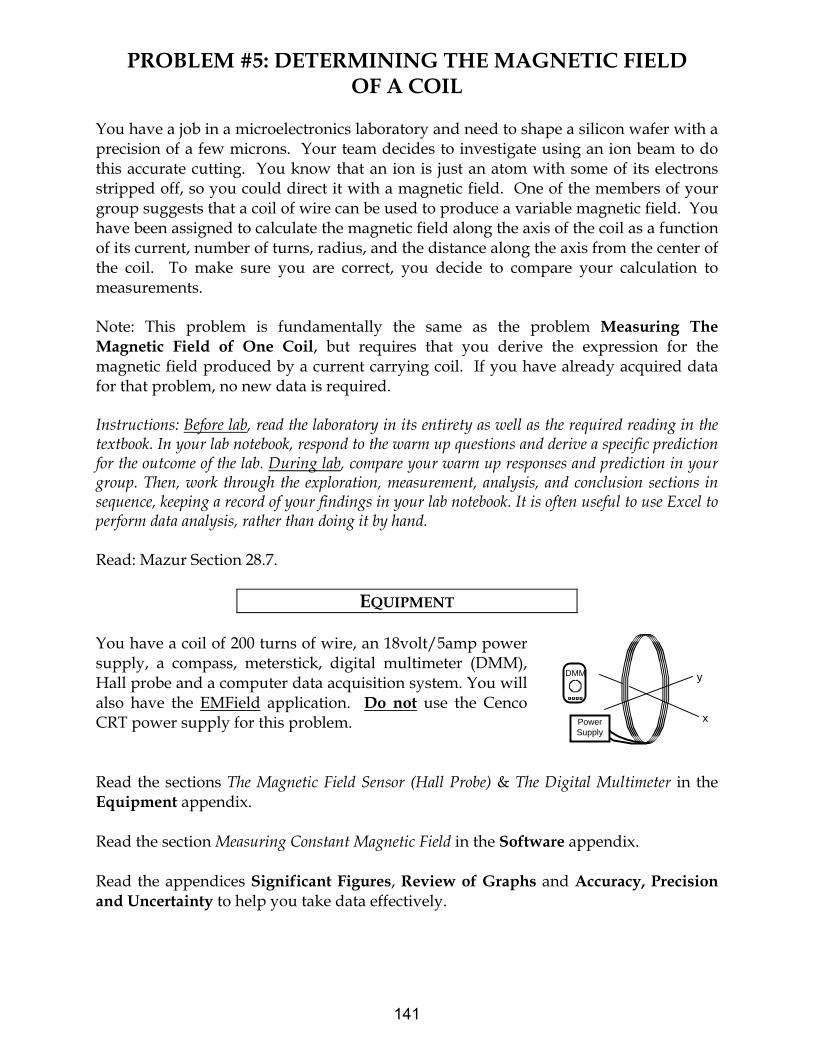
PROBLEM #5: DETERMINING THE MAGNETIC FIELD OF A COIL
You have a job in a microelectronics laboratory and need to shape a silicon wafer with a precision of a few microns. Your team decides to investigate using an ion beam to do this accurate cutting. You know that an ion is just an atom with some of its electrons stripped off, so you could direct it with a magnetic field. One of the members of your group suggests that a coil of wire can be used to produce a variable magnetic field. You have been assigned to calculate the magnetic field along the axis of the coil as a function of its current, number of turns, radius, and the distance along the axis from the center of the coil. To make sure you are correct, you decide to compare your calculation to measurements. Note: This problem is fundamentally the same as the problem Measuring The Magnetic Field of One Coil, but requires that you derive the expression for the magnetic field produced by a current carrying coil. If you have already acquired data for that problem, no new data is required. Instructions: Before lab, read the laboratory in its entirety as well as the required reading in the textbook. In your lab notebook, respond to the warm up questions and derive a specific prediction for the outcome of the lab. During lab, compare your warm up responses and prediction in your group. Then, work through the exploration, measurement, analysis, and conclusion sections in sequence, keeping a record of your findings in your lab notebook. It is often useful to use Excel to perform data analysis, rather than doing it by hand. Read: Mazur Section 28.7.
EQUIPMENT You have a coil of 200 turns of wire, an 18volt/5amp power supply, a compass, meterstick, digital multimeter (DMM), Hall probe and a computer data acquisition system. You will also have the EMField application. Do not use the Cenco CRT power supply for this problem.
Power Supply
x
yDMM
Read the sections The Magnetic Field Sensor (Hall Probe) & The Digital Multimeter in the Equipment appendix. Read the section Measuring Constant Magnetic Field in the Software appendix. Read the appendices Significant Figures, Review of Graphs and Accuracy, Precision and Uncertainty to help you take data effectively.
141

DETERMINING THE MAGNETIC FIELD OF A COIL
If equipment is missing or broken, submit a problem report by sending an email to [email protected]. Include the room number and brief description of the problem.
WARM UP 1. Make a sketch of a coil of radius R. Define a coordinate axis, label the relevant
quantities, and indicate the direction of the current through the coil.
Select a point along the axis at which you will calculate the magnetic field.
2. Select a small element of current along the coil, which will cause a small fraction of this magnetic field. Label the length of that current element. Draw a position vector from that current element to the selected point along the axis of the coil.
Use the Biot-Savart law to draw a vector representing the direction of the small part of the magnetic field from your current element at the position of interest. Determine the components of this vector along the axes of your coordinate system.
Are there any symmetries that allow you to neglect one or more components of the magnetic field at the point of interest?
3. Use the Biot-Savart law to calculate the small part of the desired component of the magnetic field, at the selected point, from the small element of current. Now add up (using an integral) all of the small fractions of that component of the magnetic field from all of the small elements of current around the coil.
Determine the magnitude of the magnetic field at that point along the axis for one loop of wire, writing your answer as a function of the distance along the axis of the coil. What will be the effect of N identical loops on the magnitude of the magnetic field?
4. Graph the magnitude of magnetic field strength as a function of the position along the central axis of the coil of wire.
PREDICTION
Calculate the magnitude of the magnetic field as a function of the position along the central axis of a coil of known radius, the number of turns of wire, and the electric current in the coil. Use this expression to graph the magnetic field strength as a function of position along the central axis of the coil.
EXPLORATION
142
DETERMINING THE MAGNETIC FIELD OF A COIL
If you have the data from Measuring The Magnetic Field of One Coil you do not necessarily need to make any additional measurements. Go directly to the analysis section. If you have not done this, continue with the exploration.
WARNING: You will be working with equipment that generates large electric voltages. Improper use can cause painful burns. To avoid danger, the power should be turned OFF and you should WAIT at least one minute before any wires are disconnected from or connected to the power supply. Never grasp a wire by its metal ends.
WARNING: Strong magnetic fields can affect pacemakers, ICDs and other implanted medical devices. Many of these devices are made with a feature that deactivates it with a magnetic field. Therefore, care must be taken to keep medical devices minimally 1’ away from any strong magnetic field.
Connect a large coil to the power supply using the adjustable voltage. Using your compass, make a qualitative map of the magnetic field produced. To get the most obvious effect on the compass, should the central axis of the coil be oriented N-S or E-W? Decide whether you should set the amplifier to high or low sensitivity. Using your compass as an indicator, adjust the current up and down to determine the sensitivity of the magnetic field to the current. For a reasonable current in the coil, use the compass to determine how far a measurable magnetic field along the axis of the coil extends. Also check out the magnetic field outside the coil. Is it large or small? Compared to what? Try reversing the current through the coil. What happens to the magnetic field at each point? Connect the Hall probe as explained in the Equipment and Software appendices. Before you push any buttons on the computer, locate the magnetic field strength window. You will notice that even when the probe is held away from obvious sources of magnetic fields, such as your bar magnets, you see a non-zero reading. From its behavior determine if this is caused by a real magnetic field or is an electronics artifact or both? If you notice an ambient field, can you determine its cause? Go through the Hall probe calibration procedure outlined in the appendix, or in the Magnetlab Guide Box in the upper right corner of the application. Be sure the sensor amplification switch on the Hall probe is set to 6.4mT range. The MagnetLab application requires the probe to be set to the 6.4mT range to work correctly. Does the Hall probe ever read a zero field? Explore the strength of the magnetic field in the plane of the coil. Is the field stronger inside or outside the coil? Where is the field the strongest inside the coil?
143

DETERMINING THE MAGNETIC FIELD OF A COIL
How far from the center of the coil along the axis can you measure the field? Is it the same on both sides of the coil? How can you tell by your magnetic field reading if you are on the axis? How far from the axis can you move the Hall probe without introducing additional uncertainty to your measurement? Write down a measurement plan.
MEASUREMENT Based on your exploration, choose a scale for your graph of magnetic field strength against position that will include all of the points you will measure. Use the Hall probe to measure the magnitude and direction of the magnetic field as a function of position along the axis of the coil. Measure the field on both sides of the coil. Be sure your Hall probe is calibrated and has the correct orientation to accurately measure the magnetic field. Make sure you take at least two measurements for averaging. Use the Hall probe to complete the field map for the coil. Use the DMM to measure the current in the coil. Try measuring the field along the axis at several different currents. If you are not familiar with a DMM see the Equipment appendix. Pay special attention to the connections and settings that are used to measure voltages and currents, and why the DMM should be connected in the circuit differently for voltage and current measurements. Do you know why we should connect them in these ways? Don't forget to measure the diameter of the coil and record the number of turns. What considerations need to be made when measuring the diameter?
ANALYSIS Graph the measured magnetic field of the coil along its axis as a function of position and compare with your prediction.
CONCLUSION Does the graph of magnetic field strength as a function of distance agree with your prediction? Is this true everywhere? Why or why not?
144
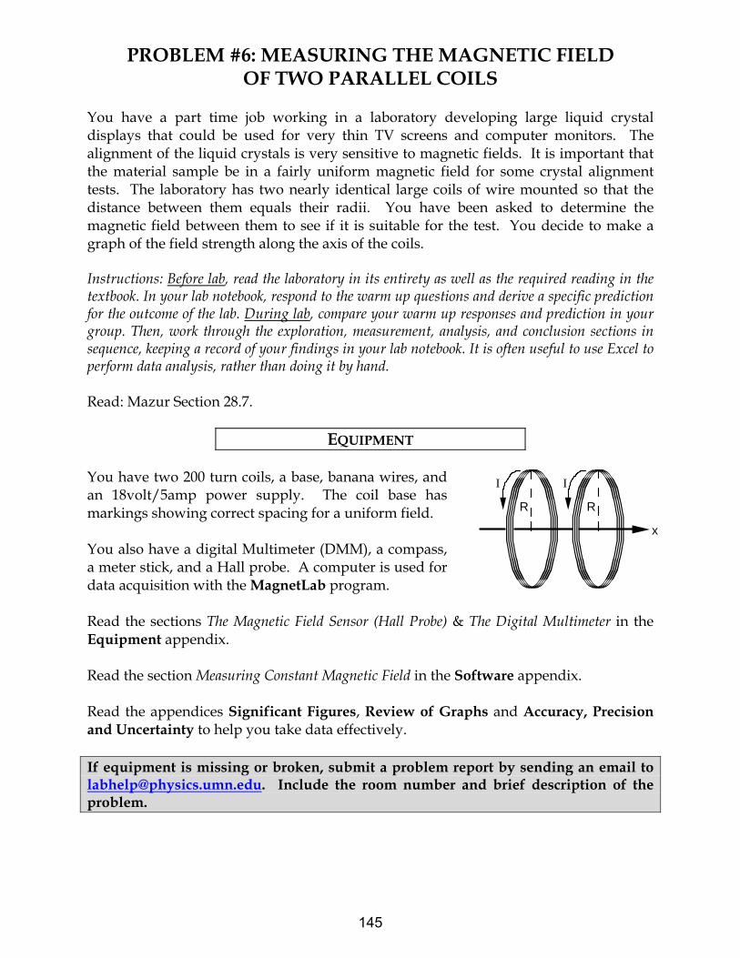
PROBLEM #6: MEASURING THE MAGNETIC FIELD OF TWO PARALLEL COILS
You have a part time job working in a laboratory developing large liquid crystal displays that could be used for very thin TV screens and computer monitors. The alignment of the liquid crystals is very sensitive to magnetic fields. It is important that the material sample be in a fairly uniform magnetic field for some crystal alignment tests. The laboratory has two nearly identical large coils of wire mounted so that the distance between them equals their radii. You have been asked to determine the magnetic field between them to see if it is suitable for the test. You decide to make a graph of the field strength along the axis of the coils. Instructions: Before lab, read the laboratory in its entirety as well as the required reading in the textbook. In your lab notebook, respond to the warm up questions and derive a specific prediction for the outcome of the lab. During lab, compare your warm up responses and prediction in your group. Then, work through the exploration, measurement, analysis, and conclusion sections in sequence, keeping a record of your findings in your lab notebook. It is often useful to use Excel to perform data analysis, rather than doing it by hand. Read: Mazur Section 28.7.
EQUIPMENT You have two 200 turn coils, a base, banana wires, and an 18volt/5amp power supply. The coil base has markings showing correct spacing for a uniform field. You also have a digital Multimeter (DMM), a compass, a meter stick, and a Hall probe. A computer is used for data acquisition with the MagnetLab program.
x
I I
R R
Read the sections The Magnetic Field Sensor (Hall Probe) & The Digital Multimeter in the Equipment appendix. Read the section Measuring Constant Magnetic Field in the Software appendix. Read the appendices Significant Figures, Review of Graphs and Accuracy, Precision and Uncertainty to help you take data effectively. If equipment is missing or broken, submit a problem report by sending an email to [email protected]. Include the room number and brief description of the problem.
145
MEASURING THE MAGNETIC FIELD OF TWO PARALLEL COILS
WARM UP
1. Draw a picture of the situation showing the direction of the current through each coil of wire. Establish a single convenient coordinate system for both coils. Label all of the relevant quantities.
2. Select a point along the axis of the two coils at which you will determine an equation for the magnetic field. In the previous problem, you calculated the magnetic field of one coil as a function of the position along its axis. To solve this problem, add the magnetic field from each coil at the selected point along the axis. Remember to pay attention to the geometry of your drawing. The origin of your coordinate system for this problem cannot be at the center of both coils at once. Also remember that the magnetic field is a vector.
3. Use your equation to graph the magnetic field strength as a function of position from the common origin along the central axis of the coils. Describe the qualitative behavior of the magnetic field between the two coils. What about the region outside the coils?
PREDICTION
Calculate the magnitude of the magnetic field for two coils as a function of the position along their central axis, for the special case where the distance between the coils is the same as the radius of the coils. Use this expression to graph the magnetic field strength versus position along the axis.
EXPLORATION
WARNING: You will be working with a power supply that can generate large electric voltages. Improper use can cause painful burns. To avoid danger, the power should be turned OFF and you should WAIT at least one minute before any wires are disconnected from or connected to the power supply. NEVER GRASP A WIRE BY ITS METAL ENDS!
WARNING: Strong magnetic fields can affect pacemakers, ICDs and other implanted medical devices. Many of these devices are made with a feature that deactivates it with a magnetic field. Therefore, care must be taken to keep medical devices minimally 1’ away from any strong magnetic field.
Connect the large coils to the power supply with the current flowing in opposite directions in the two coils, using the adjustable voltage. With the compass, explore the magnetic field produced. Be sure to look both between the coils and outside the coils.
146

MEASURING THE MAGNETIC FIELD OF TWO PARALLEL COILS
Now connect the large coils to the power supply with the current flowing in the same direction in each coil, using the adjustable voltage. With the compass, explore the magnetic field produced. Be sure to look both between the coils and outside the coils. Based on your observations, should the currents be in the same direction or in opposite directions to give the most uniform magnetic field between the coils? Connect the Hall probe according to the directions in appendices. For the current configuration that gives the most uniform magnetic field between the coils, explore the strength of the magnetic field along the axis between the coils. Follow the axis through the coils. Is the field stronger between or outside the coils? Where is the field strongest between the coils? The weakest? See how the field varies when you are between the two coils but move off the axis. How far from the axis of the coils can you measure the field? Is it the same on both sides of the coils? Decide whether to set the amplifier to high or low sensitivity. When using the MagnetLab program, consider where the zero position should be to simplify comparison with your prediction. Write down a measurement plan.
MEASUREMENT Based on your exploration, choose a scale for your graph of magnetic field strength against position that will include all of the points you will measure. Use the Hall probe to measure the magnitude of the magnetic field along the axis of the coils of wire. Be sure to measure the field on both sides of the coils. What are the units of your measured magnetic fields? How do these compare to the units of your prediction equations? Use the DMM to measure the current in the two coils. As a check, repeat these measurements with the other current configuration.
ANALYSIS Graph the measured magnetic field of the coil along its axis as a function of position and compare to your prediction.
147

MEASURING THE MAGNETIC FIELD OF TWO PARALLEL COILS
CONCLUSION
For two large, parallel coils, how does the magnetic field on the axis vary with distance along the axis? Did your measurements agree with your predictions? If not, explain. Describe the limitations on the accuracy of your measurements and analysis. Does this two-coil configuration meet the requirement of giving a fairly uniform field? Over how large a region is the field constant to within 20%? This very useful configuration of two coils (distance between coils equals radius) is called a Helmholtz coil.
148

PROBLEM #7: MAGNETS AND MOVING CHARGE
You are leading a technical team at a company that is redesigning the cathode ray tubes (CRT’s) used for computer monitors. To introduce this project to a group of stockholders, you need to demonstrate how an electron beam can be moved across a screen by a magnetic field. You decide to use an ordinary bar magnet held outside of the CRT to deflect the electrons. Before you do the demonstration, you need to know the qualitative effect of bringing a bar magnet up to a CRT. In the laboratory you qualitatively determine how the direction and size of the electron deflection is related to the magnetic field direction, the magnetic field strength, and the velocity of the electron. You also determine how the deflection is affected by how close the magnet is held to the CRT. Instructions: Before lab, read the laboratory in its entirety as well as the required reading in the textbook. In your lab notebook, respond to the warm up questions and derive a specific prediction for the outcome of the lab. During lab, compare your warm up responses and prediction in your group. Then, work through the exploration, measurement, analysis, and conclusion sections in sequence, keeping a record of your findings in your lab notebook. It is often useful to use Excel to perform data analysis, rather than doing it by hand. Read: Mazur Section 27.7. Review Deflection of an Electron Beam by an Electric Field
EQUIPMENT You have a cathode ray tube (CRT), banana cables, Cenco CRT power supply, bar magnet, a meterstick, and a compass. Read the sections Cathode Ray Tube (CRT) and Accessories and Magnetizing a Bar Magnet in the Equipment appendix. If equipment is missing or broken, submit a problem report by sending an email to [email protected]. Include the room number and brief description of the problem.
PREDICTION
If you bring the north end of a magnet near the side of the CRT, which arrow represents the deflection of the electron beam on the screen?
N
? ?
?
?
?
??
?
149
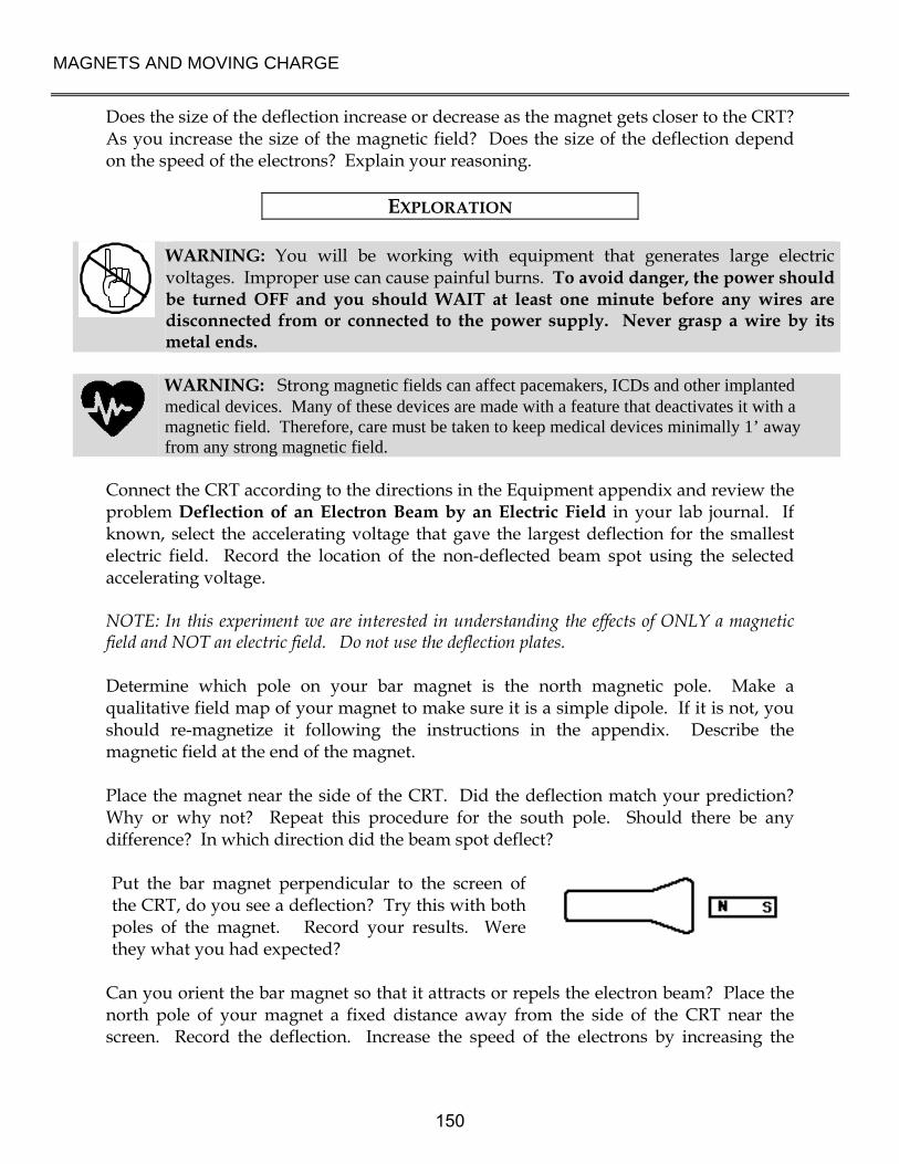
MAGNETS AND MOVING CHARGE
Does the size of the deflection increase or decrease as the magnet gets closer to the CRT? As you increase the size of the magnetic field? Does the size of the deflection depend on the speed of the electrons? Explain your reasoning.
EXPLORATION
WARNING: You will be working with equipment that generates large electric voltages. Improper use can cause painful burns. To avoid danger, the power should be turned OFF and you should WAIT at least one minute before any wires are disconnected from or connected to the power supply. Never grasp a wire by its metal ends.
WARNING: Strong magnetic fields can affect pacemakers, ICDs and other implanted medical devices. Many of these devices are made with a feature that deactivates it with a magnetic field. Therefore, care must be taken to keep medical devices minimally 1’ away from any strong magnetic field.
Connect the CRT according to the directions in the Equipment appendix and review the problem Deflection of an Electron Beam by an Electric Field in your lab journal. If known, select the accelerating voltage that gave the largest deflection for the smallest electric field. Record the location of the non-deflected beam spot using the selected accelerating voltage. NOTE: In this experiment we are interested in understanding the effects of ONLY a magnetic field and NOT an electric field. Do not use the deflection plates. Determine which pole on your bar magnet is the north magnetic pole. Make a qualitative field map of your magnet to make sure it is a simple dipole. If it is not, you should re-magnetize it following the instructions in the appendix. Describe the magnetic field at the end of the magnet. Place the magnet near the side of the CRT. Did the deflection match your prediction? Why or why not? Repeat this procedure for the south pole. Should there be any difference? In which direction did the beam spot deflect? Put the bar magnet perpendicular to the screen of the CRT, do you see a deflection? Try this with both poles of the magnet. Record your results. Were they what you had expected?
Can you orient the bar magnet so that it attracts or repels the electron beam? Place the north pole of your magnet a fixed distance away from the side of the CRT near the screen. Record the deflection. Increase the speed of the electrons by increasing the
150

MAGNETS AND MOVING CHARGE
accelerating voltage if possible. Calculate the increase in speed. How does the deflection change? Try this with both poles of the magnet. Record your results. Were your results what you had anticipated? Place the north pole of your magnet a fixed distance away from the side of the CRT near the screen. Record the deflection. Increase the magnetic field by adding a second magnet. How does the deflection change? Try this with both poles of the magnet. Record your results. Were your results what you had anticipated? What effect does the Earth’s magnetic field have on the electron beam of a CRT? What is the direction of the Earth’s magnetic field in your laboratory room? Arrange the CRT to see the maximum effect. Arrange it to observe the minimum effect. By measuring the electron deflection, what would you say is the relative strength of the magnet and the Earth’s magnetic field in the lab? Remember to take account of the distance that the electron travels through each magnetic field. What is the effect of the Earth’s magnetic field on the CRT beam relative to the Earth’s gravitational field? Devise your own exploration of the effect of a magnetic field on electrons using the CRT and the bar magnets. What variables can you control with the magnets and the CRT? Record your questions that will guide your exploration.
ANALYSIS Draw a picture relating the three vectors representing the velocity of the electron, the magnetic field, and the force on the electron that is consistent with your results.
CONCLUSION Did the electron beam deflection, in the presence of a magnetic field, agree with your prediction? Why or why not? What was the most interesting thing you learned from this exploration?
151

MAGNETS AND MOVING CHARGE
152

PROBLEM #8: MAGNETIC FORCE ON A MOVING CHARGE
You are working with a team to design a better electron microscope. To precisely control the beam of electrons, your research team decides to try a magnetic field. For your study of electron control you decide to use a Cathode Ray Tube (CRT) with a magnetic field perpendicular to its axis. From your work with Helmholtz coils in the earlier problem, Measuring the Magnetic Field in Two Parallel Coils, you know that the magnetic field between these parallel coils is fairly uniform, so you decide to use them for your test. Before you can evaluate the sensitivity of the electron microscope design, you need to determine how the magnitude of a constant magnetic field affects the position of the beam spot. Instructions: Before lab, read the laboratory in its entirety as well as the required reading in the textbook. In your lab notebook, respond to the warm up questions and derive a specific prediction for the outcome of the lab. During lab, compare your warm up responses and prediction in your group. Then, work through the exploration, measurement, analysis, and conclusion sections in sequence, keeping a record of your findings in your lab notebook. It is often useful to use Excel to perform data analysis, rather than doing it by hand. Read: Mazur Section 27.7. Review Deflection of an Electron Beam by an Electric Field
EQUIPMENT You have a cathode ray tube (CRT), digital multimeter (DMM), compass, meterstick, Helmholtz coils, banana cables, Hall probe and computer data acquisition system. The magnetic field is provided by connecting the Helmholtz coils to a power supply and placing the CRT between the coils. Read the sections Cathode Ray Tube (CRT) and Accessories, The Magnetic Field Sensor (Hall Probe) & The Digital Multimeter in the Equipment appendix. Read the section Measuring Constant Magnetic Field in the Software appendix. If equipment is missing or broken, submit a problem report by sending an email to [email protected]. Include the room number and brief description of the problem.
WARM UP 1. Draw a picture of the CRT in the Helmholtz coils. Since you will not be using electric
fields, do not include the deflection plates in your sketch. Be sure you have all the other components in your sketch. Draw a coordinate axis on this sketch and show the magnetic field direction and the region occupied by the magnetic field. Draw the electron trajectory through all regions of the CRT together with its velocity and
153

MAGNETIC FORCE ON A MOVING CHARGE
acceleration. Draw the electron trajectory if there were no magnetic field. The difference between where these two trajectories hit the CRT screen is the deflection.
2. What path does an electron follow while traveling through a constant magnetic field? The magnetic force is always perpendicular to the electron’s velocity. Are there any forces other than the magnetic force that need to be considered?
3. Determine the velocity of the electrons as they leave the electron gun in the CRT. (See your notes from the earlier problem Deflection of an Electron Beam by an Electric Field)
4. Determine the position, direction, and velocity of an electron entering the region of constant magnetic field. Determine the position, direction, and velocity of an electron as it leaves the region of constant magnetic field. What type of curve is the electron’s trajectory in that region?
5. Determine the path of the electron as it travels after it leaves the magnetic field region until it strikes the screen. Use geometry to determine how far from the center the electron strikes the screen.
PREDICTION
Write an equation for the deflection of an electron as a function of the strength of a constant magnetic field and the velocity of the electron when the direction of the magnetic field is such as to give maximum deflection. Use this equation to graph the deflection as a function of magnetic field strength for a typical electron velocity in the CRT.
EXPLORATION Review your notes from your exploration in the problem Magnets and Moving Charge.
WARNING: You will be working with a power supply that can generate large electric voltages. Improper use can cause painful burns. To avoid danger, the power should be turned OFF and you should WAIT at least one minute before any wires are disconnected from or connected to the power supply. NEVER GRASP A WIRE BY ITS METAL ENDS!
WARNING: Strong magnetic fields can affect pacemakers, ICDs and other implanted medical devices. Many of these devices are made with a feature that deactivates it with a magnetic field. Therefore, care must be taken to keep medical devices minimally 1’ away from any strong magnetic field.
Connect the CRT according to the directions in the Equipment appendix and review the problem Deflection of an electron beam by an Electric Field in your lab journal. If
154
MAGNETIC FORCE ON A MOVING CHARGE
known, select the accelerating voltage that gave the largest deflection for the smallest electric field. Record the location of the non-deflected beam spot using the selected accelerating voltage. NOTE: In this experiment we are interested in understanding the effects of ONLY a magnetic field and NOT an electric field. Do not use the deflection plates. You should have between 250 and 500 volts between the cathode and anode (Note: cathode is negative and anode is positive). After a moment, you should see a spot that you can adjust with the knob labeled “Focus”. If your connections are correct and the spot still does not appear, inform your lab instructor. The voltages listed on the CRT power supplies are approximate, you should check and measure ALL voltages AND currents with a DMM. Read the Equipment appendix if you need to review using a DMM. Devise a measuring scheme to record the position of the beam spot. Record your zero deflection position and do not move the CRT once you have started taking measurements. Review the magnetic field map from the Helmholtz Coils. Does it matter what direction the currents flows in the two Helmholtz coils? Should it be in the same direction or opposite directions? Ensure to send currents in the coils accordingly. Set up your Hall probe as explained in the Equipment and Software appendices. Before you push any buttons on the computer, locate the magnetic field strength window. You will notice that even when the probe is held away from obvious sources of magnetic fields, such as your bar magnets, you see a non-zero reading. From its behavior determine if this is caused by a real magnetic field or is an electronics artifact or both? If you notice an ambient field, can you determine its cause? Go through the Hall probe calibration procedure outlined in the appendix, or in the Magnetlab Guide Box in the upper right corner of the application. Be sure the sensor amplification switch on the Hall probe is set to 6.4mT range. The MagnetLab application requires the probe to be set to the 6.4mT range to work correctly. Does the Hall probe ever read a zero field? How will you orient the CRT with respect to the coils? Would the deflection be the same if the magnetic field were reversed? Try it. How will you determine the length of the CRT within the magnetic field? Is the field uniform throughout the flight of the electrons?
155
MAGNETIC FORCE ON A MOVING CHARGE
Write down a measurement plan.
MEASUREMENT Use the Hall Probe to Measure the magnetic field between the Helmholtz coils. Use the Hall probe to measure the magnitude and direction of the magnetic field between the coils. Measure the field near the coils. Be sure your Hall Probe is calibrated and has the correct orientation to accurately measure the magnetic field. Measure the position of the beam spot for each selected magnetic field. Make at least two measurements for averaging. The voltages listed on the CRT power supplies are approximate, you should check and measure ALL voltages AND currents with a DMM. Read the Equipment appendix if you need to review using a DMM.
ANALYSIS Graph your measurements of the deflection of the electron beam for the different values of the magnetic field at a fixed electron speed and compare to your prediction. Repeat for deflection as a function of electron speed for a fixed magnetic field.
CONCLUSION How does the deflection of the electron beam depend on the magnetic field? Did your data agree with your prediction? If not, why? What are the limitations on the accuracy of your measurements and analysis? How does the deflection of the electron beam depend on the electron speed? Did your data agree with your prediction? If not, why? What are the limitations on the accuracy of your measurements and analysis? Is controlling the deflection of an electron beam easier with a magnetic field or an electric field? Write down what you mean by easier.
156
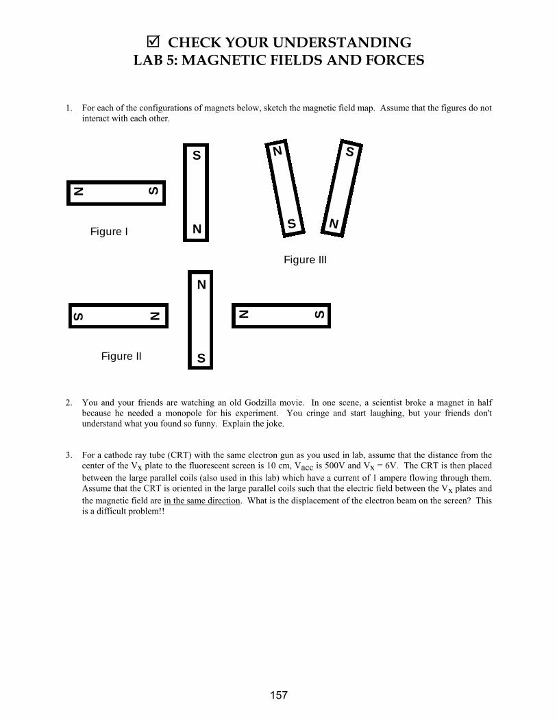
CHECK YOUR UNDERSTANDING LAB 5: MAGNETIC FIELDS AND FORCES
1. For each of the configurations of magnets below, sketch the magnetic field map. Assume that the figures do not
interact with each other.
N
S N
S
Figure III
N S
N
S
Figure I
N
S
NS
N S
Figure II
2. You and your friends are watching an old Godzilla movie. In one scene, a scientist broke a magnet in half
because he needed a monopole for his experiment. You cringe and start laughing, but your friends don't
understand what you found so funny. Explain the joke.
3. For a cathode ray tube (CRT) with the same electron gun as you used in lab, assume that the distance from the
center of the Vx plate to the fluorescent screen is 10 cm, Vacc is 500V and Vx = 6V. The CRT is then placed
between the large parallel coils (also used in this lab) which have a current of 1 ampere flowing through them.
Assume that the CRT is oriented in the large parallel coils such that the electric field between the Vx plates and
the magnetic field are in the same direction. What is the displacement of the electron beam on the screen? This
is a difficult problem!!
157

CHECK YOUR UNDERSTANDING LAB 5: MAGNETIC FIELDS AND FORCES
158

Physics Lab Report Rubric
Name: ID#:Course, Lab Sequence, and Problem Number:Date Performed:Lab Partners’ Names:
Possible Earned
Warm-Up Questions
Possible Earned
Laboratory Notebook
Earns No Points Earns Full Points Possible EarnedArgument
• no clear argument• logic does not flow• gaps in content• leaves reader with questions
• complete, cogent, flowing argument• context, execution, analysis, conclu-
sion all present• leaves reader satisfied
Technical Style
• vocabulary, syntax, etc. inappropri-ate for scientific writing
• necessary nonverbal media absent orpoorly constructed
• subjective, fanciful, or appealing toemotions
• jarringly inconsistent
• language is appropriate• nonverbal media present where ap-
propriate, well constructed, well in-corporated
• objective, indicative, logical style• consistent style• division into sections is helpful
Use of Physics
• predictions with no or with unphysi-cal justification
• experiment physically unjustified• experiment tests wrong phenomenon• theory absent from consideration of
premise, predictions, and results
• predictions are justified with physicaltheory
• experiment is physically sound andactually tests phenomenon in ques-tion
• results interpreted with theory toclear, appropriate conclusion
Quantitativeness
• statements are vague or arbitrary• analysis is inappropriately qualitative• error analysis not used to evaluate
prediction or find result• numbers, equations, units, uncertain-
ties missing or inappropriate
• consistently quantitative• equations, numbers with units, uncer-
tainties throughout• prediction confirmed or denied, result
found by error analysis• results, conclusions based on data
Total
159

160

LAB 6: ELECTRICITY FROM MAGNETISM
In the previous problems you explored the magnetic field and its effect on moving charges.
You also saw how electric currents could create magnetic fields. This lab will carry that
investigation one step further, determining how changing magnetic fields can give rise to
electric currents. This is the effect that allows the generation of electricity, which powers the
world .
The problems in this laboratory will explore d ifferent aspects of changing the magnetic flux
through a coil of wire to produce an electric current. You will investigate the current
produced in a coil of wire by moving the coil, moving the magnet causing the magnetic field ,
changing the area of the coil perpendicular to the magnetic field , and changing the magnetic
field .
OBJECTIVES:
After successfully completing this laboratory, you should be able to:
• Explain what conditions are necessary for a magnetic field to produce an electric
current.
• Determine the d irection of a current induced by a magnetic field .
• Use the concept of magnetic flux to determine the electric effects of a changing
magnetic field .
• Use Faraday's law to determine the magnitude of a potential d ifference across a wire
produced by a change of magnetic flux.
PREPARATION:
Read Mazur Chapter 29.
Before coming to lab you should be able to:
• Use a DMM to measure current, potential d ifference, and resistance.
• Sketch the magnetic fields from permanent magnets and current carrying coils of
wire.
• Use vector addition to combine magnetic fields from several sources.
• Use the right-hand rule to determine the d irection of the magnetic fields from circuit
loops and wires.
161

LAB 6: ELECTRICITY FROM MAGNETISM
• Use a Hall probe to determine the strength of a magnetic field .
• Use the definition of magnetic flux.
162

PROBLEM #1: MAGNETIC INDUCTION
One of the great technical problems in modern society is how to generate enough electricity for our growing demand. You work with a team investigating efficiency improvements for electric generators. Before becoming involved with a lot of math and computer simulations, you decide to get a feel for the problem by seeing how many different ways you can generate a potential difference with just a bar magnet and a coil of wire, and how you can influence the size of that potential difference. Instructions: Before lab, read the laboratory in its entirety as well as the required reading in the textbook. In your lab notebook, respond to the warm up questions and derive a specific prediction for the outcome of the lab. During lab, compare your warm up responses and prediction in your group. Then, work through the exploration, measurement, analysis, and conclusion sections in sequence, keeping a record of your findings in your lab notebook. It is often useful to use Excel to perform data analysis, rather than doing it by hand.
EQUIPMENT You have a small coil of wire and a bar magnet. You will use a voltage probe with software called VoltageTimeLAB.
NS
A m m e te r
Read: Mazur Sections 29.1 – 29.2. Read the section Magnetizing a Bar Magnet in the Equipment appendix if you need to re-magnetize your magnets. Read the section VoltageTimeLAB - MEASURING TIME-VARYING VOLTAGES in the Software appendix. If equipment is missing or broken, submit a problem report by sending an email to [email protected]. Include the room number and brief description of the problem.
PREDICTION Restate the problem. How many different ways can you use the magnetic field of the bar magnet to induce a potential difference across the ends of a coil of wire? Draw a diagram of each procedure that, you predict, will induce a potential difference across the ends of the coil. What do you think will influence the size of the potential difference? Explain how you arrived at your predictions.
163
MAGNETIC INDUCTION
EXPLORATION
WARNING: Strong magnetic fields can affect pacemakers, ICDs and other implanted medical devices. Many of these devices are made with a feature that deactivates it with a magnetic field. Therefore, care must be taken to keep medical devices minimally 1’ away from any strong magnetic field.
Plug the voltage probe into the SensorDAQ interface using the required Ch. 1. Attach the clips to the two ends of the coil and start the VoltageTimeLab program. Make sure you read the software appendix if necessary. Using the magnet and the coil, make sure that the apparatus is working properly and that you are getting appropriate potential difference graphs on the screen. From your predictions, how many different motions did members of your group think of to induce a potential difference across the ends of the coil? List them in your journal. Test each method and record the results. Did any method not produce a potential difference? For each method, what factors affect the magnitude and sign of the induced potential difference? Make sure everyone gets a chance to manipulate the magnet and coil and control the computer. Can you discover any methods you didn't think of earlier? What is the largest potential difference you can generate?
CONCLUSION How do your results compare with your predictions? Explain any differences, using pictures or qualitative graphs where they are helpful. State clearly the physics involved. List the important characteristics for inducing a potential difference in the coil of wire. Explain how they are related to the magnitude and sign of the induced potential difference. How do you get the largest potential difference?
164

PROBLEM #2: MAGNETIC FLUX
sYou are working on a project to build a more efficient generator. A web search reveals that most existing generators use mechanical means such as steam, water, or airflow to rotate coils of wire in a constant magnetic field. To design the generator, you need to calculate how the potential difference generated depends on the orientation of the coil with respect to the magnetic field. A colleague suggests you use the concept of magnetic flux, which involves both the magnetic field strength and the orientations of the coil and magnetic field. You decide that you need to calculate the magnetic flux through the coil as a function of the angle between the coil and the magnetic field. To help you qualitatively check your calculation, you use a computer simulation program. You then quantitatively test your calculation by modeling the situation in the laboratory. Instructions: Before lab, read the laboratory in its entirety as well as the required reading in the textbook. In your lab notebook, respond to the warm up questions and derive a specific prediction for the outcome of the lab. During lab, compare your warm up responses and prediction in your group. Then, work through the exploration, measurement, analysis, and conclusion sections in sequence, keeping a record of your findings in your lab notebook. It is often useful to use Excel to perform data analysis, rather than doing it by hand. Read: Mazur Sections 29.1 – 29.5.
EQUIPMENT Diagram of Flux Simulation screen to right. Read the sections The Magnetic Field Sensor (Hall Probe) & The Digital Multimeter in the Equipment appendix. Read the sections Flux Simulator and Measuring Constant Magnetic Field in the Software appendix.
Fr am e' sAr eaVect or
M agn et i cF i el dD i r ect i on
Fr am e
Ey e
Fr am e
Ey e' s v i ew of f l u xp assi n g t h r ou gh f r am e
165
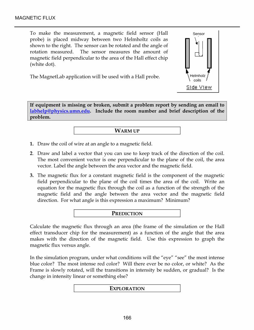
MAGNETIC FLUX
To make the measurement, a magnetic field sensor (Hall probe) is placed midway between two Helmholtz coils as shown to the right. The sensor can be rotated and the angle of rotation measured. The sensor measures the amount of magnetic field perpendicular to the area of the Hall effect chip (white dot). The MagnetLab application will be used with a Hall probe.
If equipment is missing or broken, submit a problem report by sending an email to [email protected]. Include the room number and brief description of the problem.
WARM UP 1. Draw the coil of wire at an angle to a magnetic field.
2. Draw and label a vector that you can use to keep track of the direction of the coil. The most convenient vector is one perpendicular to the plane of the coil, the area vector. Label the angle between the area vector and the magnetic field.
3. The magnetic flux for a constant magnetic field is the component of the magnetic field perpendicular to the plane of the coil times the area of the coil. Write an equation for the magnetic flux through the coil as a function of the strength of the magnetic field and the angle between the area vector and the magnetic field direction. For what angle is this expression a maximum? Minimum?
PREDICTION
Calculate the magnetic flux through an area (the frame of the simulation or the Hall effect transducer chip for the measurement) as a function of the angle that the area makes with the direction of the magnetic field. Use this expression to graph the magnetic flux versus angle. In the simulation program, under what conditions will the “eye” “see” the most intense blue color? The most intense red color? Will there ever be no color, or white? As the Frame is slowly rotated, will the transitions in intensity be sudden, or gradual? Is the change in intensity linear or something else?
EXPLORATION
Sensor
Helmholzcoils
166
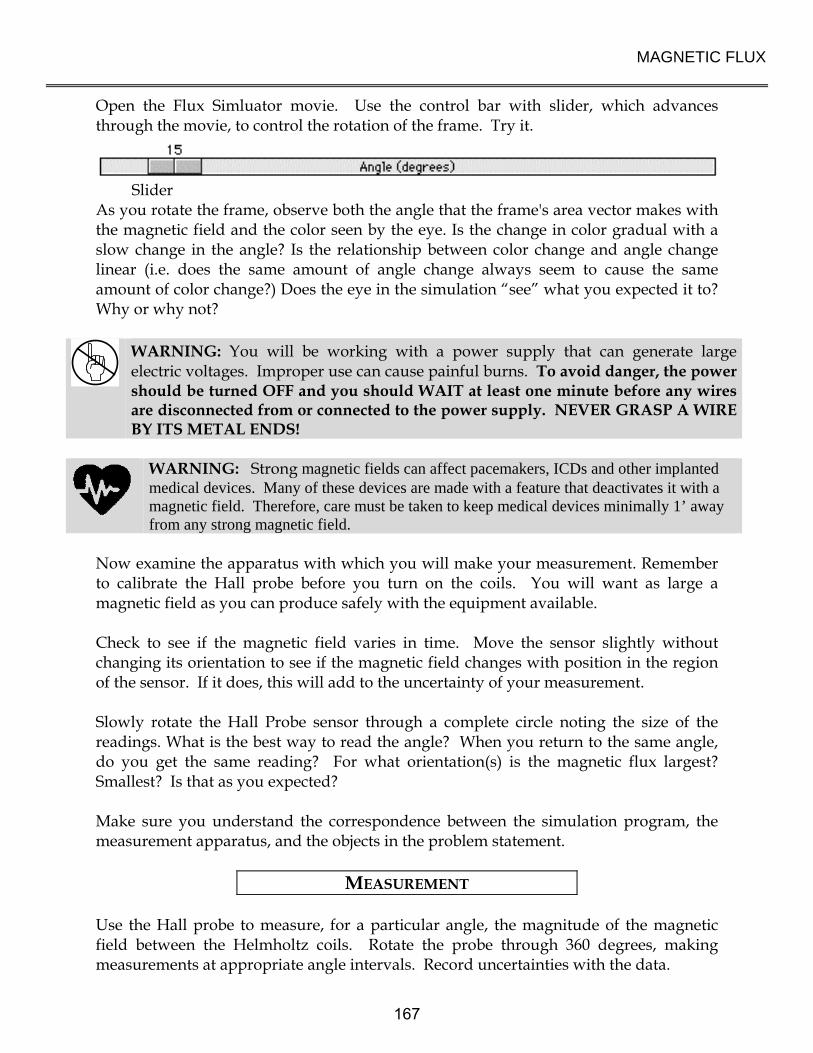
MAGNETIC FLUX
Open the Flux Simluator movie. Use the control bar with slider, which advances through the movie, to control the rotation of the frame. Try it.
Slider As you rotate the frame, observe both the angle that the frame's area vector makes with the magnetic field and the color seen by the eye. Is the change in color gradual with a slow change in the angle? Is the relationship between color change and angle change linear (i.e. does the same amount of angle change always seem to cause the same amount of color change?) Does the eye in the simulation “see” what you expected it to? Why or why not?
WARNING: You will be working with a power supply that can generate large electric voltages. Improper use can cause painful burns. To avoid danger, the power should be turned OFF and you should WAIT at least one minute before any wires are disconnected from or connected to the power supply. NEVER GRASP A WIRE BY ITS METAL ENDS!
WARNING: Strong magnetic fields can affect pacemakers, ICDs and other implanted medical devices. Many of these devices are made with a feature that deactivates it with a magnetic field. Therefore, care must be taken to keep medical devices minimally 1’ away from any strong magnetic field.
Now examine the apparatus with which you will make your measurement. Remember to calibrate the Hall probe before you turn on the coils. You will want as large a magnetic field as you can produce safely with the equipment available. Check to see if the magnetic field varies in time. Move the sensor slightly without changing its orientation to see if the magnetic field changes with position in the region of the sensor. If it does, this will add to the uncertainty of your measurement. Slowly rotate the Hall Probe sensor through a complete circle noting the size of the readings. What is the best way to read the angle? When you return to the same angle, do you get the same reading? For what orientation(s) is the magnetic flux largest? Smallest? Is that as you expected? Make sure you understand the correspondence between the simulation program, the measurement apparatus, and the objects in the problem statement.
MEASUREMENT Use the Hall probe to measure, for a particular angle, the magnitude of the magnetic field between the Helmholtz coils. Rotate the probe through 360 degrees, making measurements at appropriate angle intervals. Record uncertainties with the data.
167

MAGNETIC FLUX
ANALYSIS
Describe the color and intensity change seen by the eye as the frame rotates. What does this represent? After the Hall probe measurement, choose an equation, based on your prediction, that best represents your data points and adjust the coefficients to get the best correspondence with the data.
CONCLUSION How is the magnetic flux through the coil dependent on the angle it makes with the magnetic field? Is the flux ever zero? When is the flux a maximum? How did the results compare to your prediction?
168

PROBLEM #3: THE SIGN OF THE INDUCED POTENTIAL DIFFERENCE
For the next polar expedition, your engineering firm has developed an electric generator that can operate in extreme conditions. The expedition team is convinced that they need to understand generators, “just in case one breaks.” You find yourself trying to describe to the leader how the sign of the induced potential difference across the ends of a coil of wire depends on the physical arrangement and relative motions of the materials. You decide to do a quick demonstration with the simplest situation possible; you first push the north pole of a bar magnet through the coil, and then you repeat with the south pole of the magnet. What happens? What else could you do with the same equipment? Instructions: Before lab, read the laboratory in its entirety as well as the required reading in the textbook. In your lab notebook, respond to the warm up questions and derive a specific prediction for the outcome of the lab. During lab, compare your warm up responses and prediction in your group. Then, work through the exploration, measurement, analysis, and conclusion sections in sequence, keeping a record of your findings in your lab notebook. It is often useful to use Excel to perform data analysis, rather than doing it by hand. Read: Mazur Sections 29.1 – 29.2 and 29.4.
EQUIPMENT
You have a small coil of wire and a bar magnet. You will use the voltage probe with the VoltageTimeLAB software.
NS
Ammet er
Read the section Magnetizing a Bar Magnet in the Equipment appendix if you need to re-magnetize your magnets. Read the section VoltageTimeLAB - MEASURING TIME-VARYING VOLTAGES in the Software appendix. If equipment is missing or broken, submit a problem report by sending an email to [email protected]. Include the room number and brief description of the problem.
169

THE SIGN OF THE INDUCED POTENTIAL DIFFERENCE
WARM UP
1. Draw a picture of each situation. Draw and label the velocity vector of the magnet relative to the coil. Also draw the direction of the magnetic field vectors in the coil.
2. Use Lenz’s Law to relate the changing flux through the coil to the sign of the potential difference induced across the ends of the coil? How does the induced potential difference across the ends of the coil relate to the induced current in the coil?
PREDICTION
Restate the problem. How do you determine the sign of the induced potential difference across the ends of a coil of wire?
EXPLORATION
WARNING: Strong magnetic fields can affect pacemakers, ICDs and other implanted medical devices. Many of these devices are made with a feature that deactivates it with a magnetic field. Therefore, care must be taken to keep medical devices minimally 1’ away from any strong magnetic field.
Plug the voltage probe into the SensorDAQ interface using the required Ch. 1. Attach the clips to the two ends of the coil and start the VoltageTimeLab program. Make sure you read the software appendix if necessary. Using the magnet and the coil, make sure that the apparatus is working properly and that you are getting appropriate potential difference graphs on the screen. Push one end of the magnet into the coil and note the sign of the induced potential difference. Is the sign of the induced potential difference the same if you hold the magnet steady and instead move the coil? How does changing the velocity of the moving magnet (or the moving coil) change the magnitude and sign of the induced potential difference? How does the sign of the induced potential difference change when you (i) push the magnet into the coil; (ii) leave it in the coil without moving, and iii) pull it out of the coil? What happens if you move the magnet next to the coil? Try it.
170

THE SIGN OF THE INDUCED POTENTIAL DIFFERENCE
MEASUREMENT Determine the sign of induced potential difference across the ends of the coil when you push the north pole of the magnet through the coil and when you push the south pole of the magnet through the coil. Repeat the measurements, but this time keep the magnet still and move the coil.
CONCLUSION
Did your results agree with your predictions? Explain any differences.
171

THE SIGN OF THE INDUCED POTENTIAL DIFFERENCE
172

PROBLEM #4: THE MAGNITUDE OF THE INDUCED POTENTIAL DIFFERENCE
You’re part of a team designing a bicycle speedometer. It is a circuit with a small pick-up coil on the bicycle’s front fork, near the wheel’s axle. When riding the bike, a tiny magnet attached to one of the spokes passes by the coil and induces a potential difference in the coil. That potential difference is read by a detector, which sends the information to the speedometer. You wonder how fast the bike must move to produce a detectable signal. You decide to model the situation by calculating how the induced potential difference across the ends of a coil of wire depends on the velocity with which a magnet is thrust through it. To check your calculation, you set up a laboratory model in which you can systematically vary the speed of the magnet by mounting it on a cart and rolling the cart down a ramp from different positions on the ramp. At the end of the ramp, the cart passes through the center of a coil of wire. Instructions: Before lab, read the laboratory in its entirety as well as the required reading in the textbook. In your lab notebook, respond to the warm up questions and derive a specific prediction for the outcome of the lab. During lab, compare your warm up responses and prediction in your group. Then, work through the exploration, measurement, analysis, and conclusion sections in sequence, keeping a record of your findings in your lab notebook. It is often useful to use Excel to perform data analysis, rather than doing it by hand. Read: Mazur Section 29.5.
EQUIPMENT
You have a coil of 200 turns of wire, a magnet, meterstick, cart, and track. The track is raised at an incline using wooden blocks. You also have voltage probe with software called VoltageTimeLAB.
Table
M agnet
C art
C oil
Track
Table
Read the section Magnetizing a Bar Magnet in the Equipment appendix if you need to re-magnetize your magnets. Read the section VoltageTimeLAB - MEASURING TIME-VARYING VOLTAGES in the Software appendix. If equipment is missing or broken, submit a problem report by sending an email to [email protected]. Include the room number and brief description of the problem.
173
THE MAGNITUDE OF THE INDUCED POTENTIAL DIFFERENCE
WARM UP
1. Draw a picture of the situation. Label important distances and kinematic quantities. Decide on an appropriate coordinate system and add it to your picture.
2. Use Faraday’s Law to relate change of magnetic flux to the magnitude of the induced potential difference in the coil.
3. Draw a magnetic field map of a bar magnet. Draw the coil of wire on the magnetic field map. As the bar magnet passes through the coil, when is the flux change the strongest? What is the relationship between the velocity of the bar magnet and the change of the magnetic flux through the coil? This tells you, qualitatively how the flux changes with time.
4. Look at the time rate change of the magnetic flux. How is it related to the velocity of the cart? It is important to note whether or not the quantities of interest vary with time or with the cross-sectional area of the coil.
5. What physics principles can you use to determine the velocity of the magnet as it passes through the coil to the starting position of the cart?
6. Write an equation giving the induced potential difference across the ends of the coil of wire as a function of the velocity of the magnet through the coil.
7. Write an expression for the velocity of the cart through the coil as a function of its starting distance from the coil. Substitute that into the equation for the induced emf.
PREDICTION
Calculate the induced potential difference in the coil as a function of the distance from the coil at which the cart is released and other quantities that are not changed. Make a graph of this function.
EXPLORATION
WARNING: Strong magnetic fields can affect pacemakers, ICDs and other implanted medical devices. Many of these devices are made with a feature that deactivates it with a magnetic field. Therefore, care must be taken to keep medical devices minimally 1’ away from any strong magnetic field. The PASCO carts have neodymium magnets inside of them that have very strong fields.
Before you begin exploring, consider what the signal displayed by the VoltagetimeLab program will look like. Will you be able to tell by the signal when the cart has not passed through the ring, and when it has? Will the peaks be sharp or rounded? Will there be many peaks or only one? How will the signal look different from background noise? Draw on your experiences from problems 1 and 3 in this lab.
174
THE MAGNITUDE OF THE INDUCED POTENTIAL DIFFERENCE
Plug the voltage probe into the SensorDAQ interface using the required Ch. 1. Attach the clips to the two ends of the coil and start the VoltageTimeLab program. Make sure you read the software appendix if necessary. Push the bar magnet through the coil to make sure that the apparatus is working properly and that you are getting appropriate signal on the screen. How does the graph compare to your expectations? Make sure you can freeze the screen while showing your desired data. Set up the track at an incline so that a rolling cart will go through the center of the coil. Try different angles to get the most reproducible situation in which you can change the velocity of the cart over the widest range without damaging the equipment. Be sure to have someone catch the cart when it reaches the end of the incline. Securely attach a bar magnet to the cart and let it roll down the track while observing the potential difference displayed by the computer. Check that the release position does affect the potential difference graph on the computer. Try different time scales over which the computer makes the measurement. Are the differences large enough to measure reliably? Does the orientation of the magnet matter? Try different orientations. Do the magnetic bumpers in the cart matter? Try a cart without a bar magnet. Does the display of the potential difference as a function of time on the computer look as you expected? Be sure you can qualitatively explain the behavior that you see displayed. You might want to move the magnet by hand to see if your understanding is correct. Try adding another bar magnet to the cart to increase the magnitude of the induced potential difference. Does it matter how the second magnet is oriented? Develop a measurement plan to take the data you need to answer the question.
MEASUREMENT Follow your measurement plan and record the maximum potential difference across the ends of the coil of wire as a function of the velocity of the magnet through the coil.
175

THE MAGNITUDE OF THE INDUCED POTENTIAL DIFFERENCE
ANALYSIS
From your data construct a graph of maximum induced potential difference in the coil as a function of the distance from the coil at which the cart is released. Add the graph of your prediction to the same plot and compare. You may need to normalize the graphs.
CONCLUSION
Did your results agree with your predictions? Explain any differences. From the computer screen, make a sketch of the shape of the induced potential difference across the ends of the coil as a function of time for one pass of the magnet. Label each feature of the graph and indicate where the magnet is in the coil at that time and why the graph looks like it does at that time.
176

PROBLEM #5: THE GENERATOR
To begin investigating how to improve the efficiency of electric generators, your supervisor assigns you the task of building a working model of a generator from which it is easy to take measurements. Your model consists of Helmholtz coils to generate a well-defined magnetic field and a smaller coil of wire, in between the Helmholtz coils, to generate the current. The small coil is mounted to a motor so that it spins at a uniform speed. Before presenting the model to your supervisor you calculate the potential difference you expect and then take some measurements to make sure that the results correspond to your understanding of the situation. You will need to determine how the expected potential difference may depend on time, the rate of small coil rotation, and other parameters in your setup. Instructions: Before lab, read the laboratory in its entirety as well as the required reading in the textbook. In your lab notebook, respond to the warm up questions and derive a specific prediction for the outcome of the lab. During lab, compare your warm up responses and prediction in your group. Then, work through the exploration, measurement, analysis, and conclusion sections in sequence, keeping a record of your findings in your lab notebook. It is often useful to use Excel to perform data analysis, rather than doing it by hand. Read: Mazur Section 29.5 and Example 29.6.
EQUIPMENT The small coil mounts to the base between the Helmholtz coils, as shown to the right. The Helmholtz coils are connected to a power supply. The small coil is labeled with the # turns of wire, and can be rotated by a motor. DO NOT connect a power supply to the small coil or you will damage it. You will have a Hall probe, a DMM, and a meterstick. You will also have a voltage probe with the VoltageTimeLAB software.
small coil
Helmholzcoils
Read the sections The Magnetic Field Sensor (Hall Probe) & The Digital Multimeter in the Equipment appendix. Read the sections VoltageTimeLAB - MEASURING TIME-VARYING VOLTAGES and Measuring Constant Magnetic Field in the Software appendix. If equipment is missing or broken, submit a problem report by sending an email to [email protected]. Include the room number and brief description of the problem.
177

THE GENERATOR
WARM UP
1. Draw a picture of the equipment labeling the direction of the magnetic field and the orientation of the small coil. Choose a coordinate system on the small coil.
2. Use Faraday’s Law to relate the changing magnetic flux through the coil to the potential difference across the ends of the coil of wire. The changing magnetic flux is caused by the angular speed of the coil.
3. Draw a diagram showing only the small coil, a vector giving the direction of the magnetic field, and the area vector for the coil.
4. Write an equation for the magnetic flux through the small coil when it is stationary and at some angle to the magnetic field.
As the small coil is rotated, how does the angle its area vector makes with the magnetic field vary with time? That variation is related to its angular speed.
5. Write an expression for the change in magnetic flux through the small coil as it turns.
PREDICTION Calculate the potential difference produced by a coil of wire spinning in a uniform magnetic field as a function of its angular speed.
EXPLORATION
WARNING: You will be working with a power supply that can generate large electric voltages. Improper use can cause painful burns. To avoid danger, the power should be turned OFF and you should WAIT at least one minute before any wires are disconnected from or connected to the power supply. NEVER GRASP A WIRE BY ITS METAL ENDS!
WARNING: Strong magnetic fields can affect pacemakers, ICDs and other implanted medical devices. Many of these devices are made with a feature that deactivates it with a magnetic field. Therefore, care must be taken to keep medical devices minimally 1’ away from any strong magnetic field.
You will want the largest magnetic field you can produce safely with the equipment. Develop a plan for measuring the magnetic field using the Hall probe and Magnetlab application. Where will you want to measure the magnetic field? Over what region do you need the magnetic field to be reasonably constant? Check to see if it is.
178
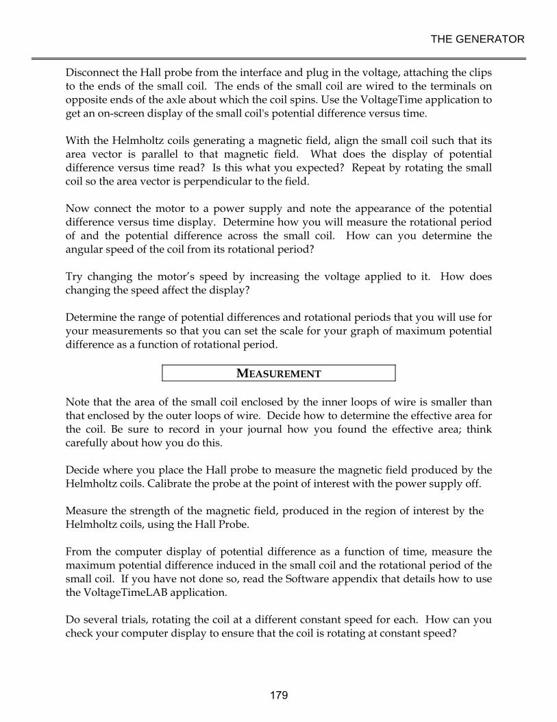
THE GENERATOR
Disconnect the Hall probe from the interface and plug in the voltage, attaching the clips to the ends of the small coil. The ends of the small coil are wired to the terminals on opposite ends of the axle about which the coil spins. Use the VoltageTime application to get an on-screen display of the small coil's potential difference versus time. With the Helmholtz coils generating a magnetic field, align the small coil such that its area vector is parallel to that magnetic field. What does the display of potential difference versus time read? Is this what you expected? Repeat by rotating the small coil so the area vector is perpendicular to the field. Now connect the motor to a power supply and note the appearance of the potential difference versus time display. Determine how you will measure the rotational period of and the potential difference across the small coil. How can you determine the angular speed of the coil from its rotational period? Try changing the motor’s speed by increasing the voltage applied to it. How does changing the speed affect the display? Determine the range of potential differences and rotational periods that you will use for your measurements so that you can set the scale for your graph of maximum potential difference as a function of rotational period.
MEASUREMENT Note that the area of the small coil enclosed by the inner loops of wire is smaller than that enclosed by the outer loops of wire. Decide how to determine the effective area for the coil. Be sure to record in your journal how you found the effective area; think carefully about how you do this. Decide where you place the Hall probe to measure the magnetic field produced by the Helmholtz coils. Calibrate the probe at the point of interest with the power supply off. Measure the strength of the magnetic field, produced in the region of interest by the Helmholtz coils, using the Hall Probe. From the computer display of potential difference as a function of time, measure the maximum potential difference induced in the small coil and the rotational period of the small coil. If you have not done so, read the Software appendix that details how to use the VoltageTimeLAB application. Do several trials, rotating the coil at a different constant speed for each. How can you check your computer display to ensure that the coil is rotating at constant speed?
179

THE GENERATOR
ANALYSIS Determine the equation that best represents your collected data. What physical quantities do the constants in your equation represent? What do the variables in your equation represent?
CONCLUSION What is the potential difference induced in a coil spinning in a uniform magnetic field? Did your measured potential difference agree with the predicted potential difference? Did the period of the signal agree with your predictions? If not, why not? What are the limitations on the accuracy of your measurements and analysis? How does the amount of potential difference produced by the generator depend on the angular speed at which the generator rotates?
180
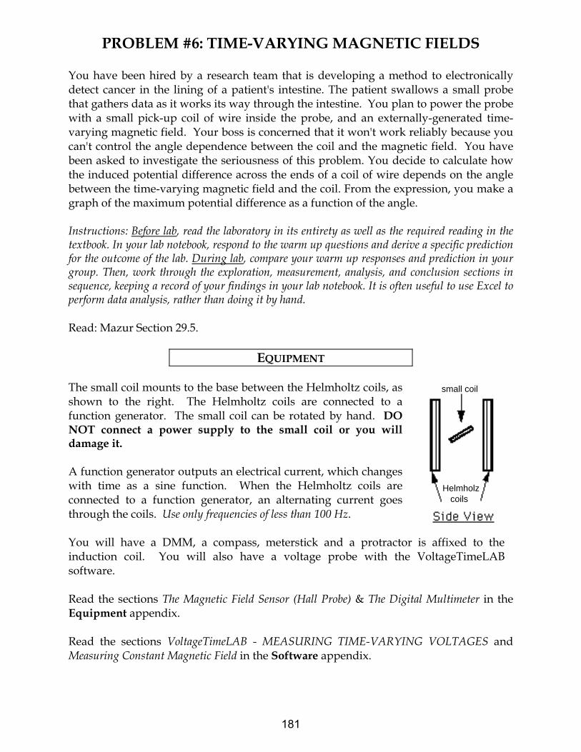
PROBLEM #6: TIME-VARYING MAGNETIC FIELDS
You have been hired by a research team that is developing a method to electronically detect cancer in the lining of a patient's intestine. The patient swallows a small probe that gathers data as it works its way through the intestine. You plan to power the probe with a small pick-up coil of wire inside the probe, and an externally-generated time-varying magnetic field. Your boss is concerned that it won't work reliably because you can't control the angle dependence between the coil and the magnetic field. You have been asked to investigate the seriousness of this problem. You decide to calculate how the induced potential difference across the ends of a coil of wire depends on the angle between the time-varying magnetic field and the coil. From the expression, you make a graph of the maximum potential difference as a function of the angle. Instructions: Before lab, read the laboratory in its entirety as well as the required reading in the textbook. In your lab notebook, respond to the warm up questions and derive a specific prediction for the outcome of the lab. During lab, compare your warm up responses and prediction in your group. Then, work through the exploration, measurement, analysis, and conclusion sections in sequence, keeping a record of your findings in your lab notebook. It is often useful to use Excel to perform data analysis, rather than doing it by hand. Read: Mazur Section 29.5.
EQUIPMENT The small coil mounts to the base between the Helmholtz coils, as shown to the right. The Helmholtz coils are connected to a function generator. The small coil can be rotated by hand. DO NOT connect a power supply to the small coil or you will damage it. A function generator outputs an electrical current, which changes with time as a sine function. When the Helmholtz coils are connected to a function generator, an alternating current goes through the coils. Use only frequencies of less than 100 Hz.
small coil
Helmholzcoils
You will have a DMM, a compass, meterstick and a protractor is affixed to the induction coil. You will also have a voltage probe with the VoltageTimeLAB software. Read the sections The Magnetic Field Sensor (Hall Probe) & The Digital Multimeter in the Equipment appendix. Read the sections VoltageTimeLAB - MEASURING TIME-VARYING VOLTAGES and Measuring Constant Magnetic Field in the Software appendix.
181

TIME-VARYING MAGNETIC FIELDS
If equipment is missing or broken, submit a problem report by sending an email to [email protected]. Include the room number and brief description of the problem.
WARM UP
1. Draw a picture of the equipment, labeling the direction of the magnetic field and the orientation of the small coil. Choose a coordinate system on the small coil.
2. Use Faraday’s Law to relate the changing magnetic flux (by the Helmholtz coils) through the induction coil to the potential difference across the ends of the coil of wire.
3. Draw a diagram showing only the small coil, a vector giving the direction of the magnetic field, and the area vector for the coil. Write an equation relating the magnetic flux through the small coil, when it is stationary and at some angle to the magnetic field, to the strength of the magnetic field.
4. Write an equation for the magnetic field produced by the current in the Helmholtz coils, assuming the current through the Helmholtz coils varies with time as a sine function.
5. Write an expression for the change in magnetic flux through the small coil.
6. Combine the expressions you have written to write an expression for the time-varying potential difference across the ends of the small coil at some angle to the magnetic field. Use that result to write an expression for the maximum potential difference across the ends of the coil at any particular angle and graph the maximum potential difference vs. the angle.
PREDICTION
Calculate the potential difference across the pick-up coil, for a magnetic field changing with a known period, as a function of the angle the coil makes with the magnetic field. From this expression, make a graph of the maximum potential difference as a function of the angle.
EXPLORATION
WARNING: Strong magnetic fields can affect pacemakers, ICDs and other implanted medical devices. Many of these devices are made with a feature that deactivates it with a magnetic field. Therefore, care must be taken to keep medical devices minimally 1’ away from any strong magnetic field.
182

TIME-VARYING MAGNETIC FIELDS
Use the function generator to drive a low frequency AC current through the large parallel coils:
Set the function generator to create a sinusoidal voltage. Set the frequency of the function generator to less than 100 Hertz. Use the output labeled LO on the function generator to drive the current
through the coils. Set the amplitude of the function generator near its maximum. Connect the Helmholtz coils in series so that they carry the same current. Check
to see which way the current is going in each coil. Does it matter? If you placed a compass in the magnetic field near the pick-up coil, what would you expect to see? Try it. Slowly increase the frequency of the current in the Helmholtz coils. What happens to the compass needle? Is this consistent with what you expected? Use the Hall probe to measure the magnetic field near the pick-up coil. What do you observe? Reduce the frequency setting on the function generator if necessary to more clearly see the behavior of the magnetic field. Position the Hall probe to measure the maximum magnetic field and note the range of values you find. Orient the pick-up coil so that the largest magnetic flux passes through it. Attach the DMM to the pick-up coil set to read AC voltage. Increase the frequency on the function generator to about 60 Hertz. Slowly change the orientation of the pick-up coil to see how the AC voltage varies. Attach the voltage probe to the pick-up coil to read the potential difference across it. Use the VoltagetimeLab application to view the potential difference as a function of time. Choose a frequency and amplitude setting on the function generator to produce a clean plot. Select a range of angles to use in your measurement and note the range of potential difference amplitudes you expect for the signal generator frequency and amplitude you have chosen to use.
MEASUREMENT For a fixed function generator output, measure how the amplitude of the potential difference across the pick-up coil varies as a function of its angle with the magnetic field. Take data sufficient to convince others of your findings.
183

TIME-VARYING MAGNETIC FIELDS
ANALYSIS
Using your measurements, graph the potential difference across the pick-up coil as a function of time, for a fixed function generator output. What is the period of the potential difference? The frequency? How does this behavior change as the angle between the pick-up coil and the magnetic field changes? How does the time structure of the induced potential compare to the output of the function generator? Graph the maximum potential difference across the pick-up coil as a function of the angle the coil's area vector makes with the magnetic field.
CONCLUSION Does the time variation of the potential difference across the pick-up coil agree with your prediction? If not, why? Highlight the similarity and differences with the previous problem, The Generator.
184

CHECK YOUR UNDERSTANDING LAB 6: ELECTRICITY FROM MAGNETISM
1. A long solenoid, with the axis perpendicular to the plane of the paper, carries a current that continually
increases with time. A loop of wire with two light bulbs is connected around the solenoid. What is the
direction of the induced current in the wire loop? Compare the brightness of light bulbs 1 and 2.
A
B
1
2
Magnetic f ield
increasing
into plane of
paper
Light bulb
Wire loop
If a wire was connected from point A to point B, compare the brightness of bulbs 1 and 2.
2. A coil with 50 turns, a diameter of 8 cm, and a resistance of 9 is placed perpendicular to a uniform
magnetic field of 2.0 T. The magnetic field suddenly reverses direction. What is the total charge that
passes through the coil?
185

CHECK YOUR UNDERSTANDING LAB 6: ELECTRICITY FROM MAGNETISM
186

Physics Lab Report Rubric
Name: ID#:Course, Lab Sequence, and Problem Number:Date Performed:Lab Partners’ Names:
Possible Earned
Warm-Up Questions
Possible Earned
Laboratory Notebook
Earns No Points Earns Full Points Possible EarnedArgument
• no clear argument• logic does not flow• gaps in content• leaves reader with questions
• complete, cogent, flowing argument• context, execution, analysis, conclu-
sion all present• leaves reader satisfied
Technical Style
• vocabulary, syntax, etc. inappropri-ate for scientific writing
• necessary nonverbal media absent orpoorly constructed
• subjective, fanciful, or appealing toemotions
• jarringly inconsistent
• language is appropriate• nonverbal media present where ap-
propriate, well constructed, well in-corporated
• objective, indicative, logical style• consistent style• division into sections is helpful
Use of Physics
• predictions with no or with unphysi-cal justification
• experiment physically unjustified• experiment tests wrong phenomenon• theory absent from consideration of
premise, predictions, and results
• predictions are justified with physicaltheory
• experiment is physically sound andactually tests phenomenon in ques-tion
• results interpreted with theory toclear, appropriate conclusion
Quantitativeness
• statements are vague or arbitrary• analysis is inappropriately qualitative• error analysis not used to evaluate
prediction or find result• numbers, equations, units, uncertain-
ties missing or inappropriate
• consistently quantitative• equations, numbers with units, uncer-
tainties throughout• prediction confirmed or denied, result
found by error analysis• results, conclusions based on data
Total
187

188

Appendix: EQUIPMENT
ELECTROSTATIC PAPER AND ACCESSORIES:
To investigate electric fields with the electrostatic paper, you need to do the following: • Lay the electrostatic paper flat. . • Distribute the pieces of metal (called “electrodes”) on the paper, in the configuration whose field
you wish to examine. The tips of the long brass rods may also be used as electrodes, to create point-like charges.
• Connect the electrodes to a source of charge. This is done by connecting a wire from the positive (“+”) side of the battery or power supply to one electrode and the wire from the negative (“–”) side to the other as shown in Figure 1.
• You may wish to place a wooden block on top of the brass rods to increase contact pressure with the paper. This can increase the magnitude of the electric field created on the paper. It also helps to place an extra sheet of paper under the electrostatic paper.
Figure 1: Electrostatic paper Setup Figure 2: Electric Field Probe
To measure the electric field from the charged electrodes, you will use a probe connected to a digital Multimeter set to measure volts (see Figure 2). For best results, turn the DMM to measure in the two-volt DC range, as indicated in Figure 2.
189
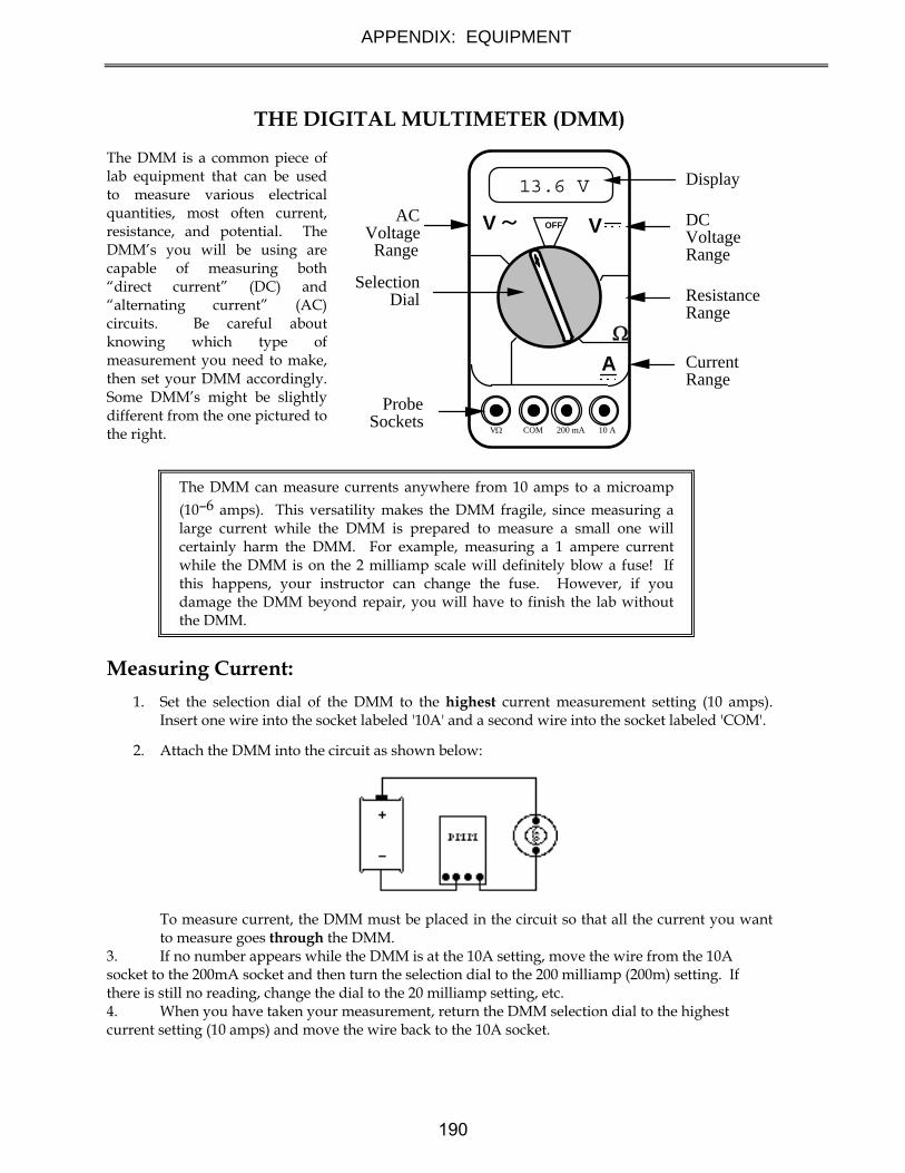
APPENDIX: EQUIPMENT
THE DIGITAL MULTIMETER (DMM) The DMM is a common piece of lab equipment that can be used to measure various electrical quantities, most often current, resistance, and potential. The DMM’s you will be using are capable of measuring both “direct current” (DC) and “alternating current” (AC) circuits. Be careful about knowing which type of measurement you need to make, then set your DMM accordingly. Some DMM’s might be slightly different from the one pictured to the right.
The DMM can measure currents anywhere from 10 amps to a microamp
(10–6 amps). This versatility makes the DMM fragile, since measuring a large current while the DMM is prepared to measure a small one will certainly harm the DMM. For example, measuring a 1 ampere current while the DMM is on the 2 milliamp scale will definitely blow a fuse! If this happens, your instructor can change the fuse. However, if you damage the DMM beyond repair, you will have to finish the lab without the DMM.
Measuring Current:
1. Set the selection dial of the DMM to the highest current measurement setting (10 amps). Insert one wire into the socket labeled '10A' and a second wire into the socket labeled 'COM'.
2. Attach the DMM into the circuit as shown below:
To measure current, the DMM must be placed in the circuit so that all the current you want to measure goes through the DMM.
3. If no number appears while the DMM is at the 10A setting, move the wire from the 10A socket to the 200mA socket and then turn the selection dial to the 200 milliamp (200m) setting. If there is still no reading, change the dial to the 20 milliamp setting, etc. 4. When you have taken your measurement, return the DMM selection dial to the highest current setting (10 amps) and move the wire back to the 10A socket.
13.6 V
V~ OFF
A
V
V 10 A200 mACOM
Display
AC Voltage Range
DC Voltage Range
Resistance Range
Current Range
Selection Dial
Probe Sockets
190
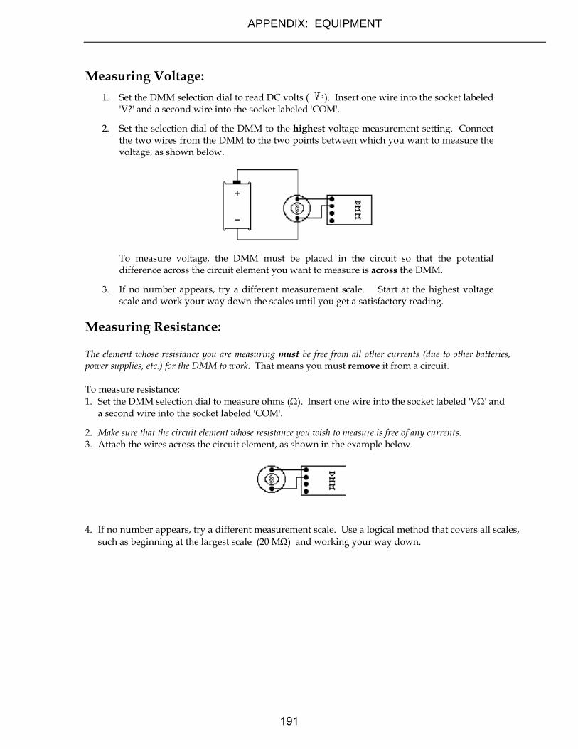
APPENDIX: EQUIPMENT
Measuring Voltage:
1. Set the DMM selection dial to read DC volts ( ). Insert one wire into the socket labeled 'V?' and a second wire into the socket labeled 'COM'.
2. Set the selection dial of the DMM to the highest voltage measurement setting. Connect the two wires from the DMM to the two points between which you want to measure the voltage, as shown below.
To measure voltage, the DMM must be placed in the circuit so that the potential difference across the circuit element you want to measure is across the DMM.
3. If no number appears, try a different measurement scale. Start at the highest voltage scale and work your way down the scales until you get a satisfactory reading.
Measuring Resistance: The element whose resistance you are measuring must be free from all other currents (due to other batteries, power supplies, etc.) for the DMM to work. That means you must remove it from a circuit. To measure resistance: 1. Set the DMM selection dial to measure ohms (). Insert one wire into the socket labeled 'V' and
a second wire into the socket labeled 'COM'.
2. Make sure that the circuit element whose resistance you wish to measure is free of any currents. 3. Attach the wires across the circuit element, as shown in the example below.
4. If no number appears, try a different measurement scale. Use a logical method that covers all scales,
such as beginning at the largest scale (20 M) and working your way down.
191
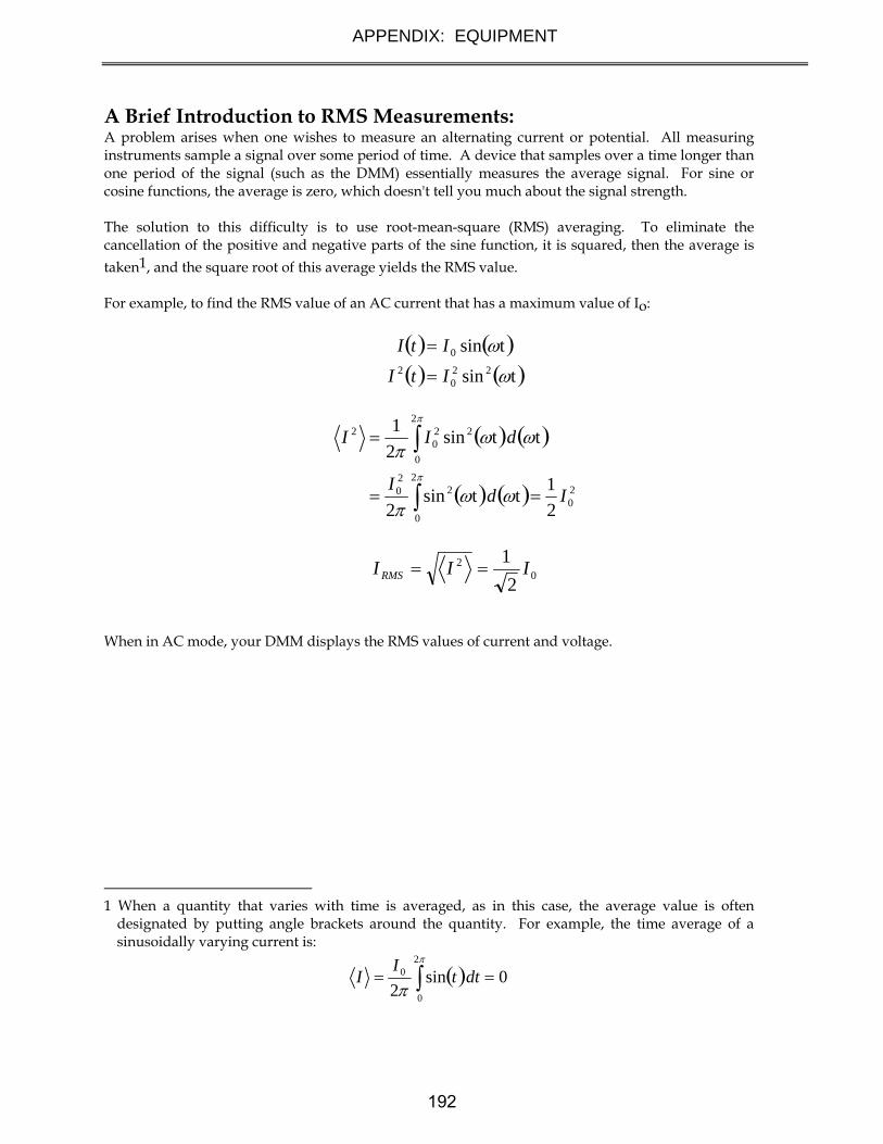
APPENDIX: EQUIPMENT
A Brief Introduction to RMS Measurements: A problem arises when one wishes to measure an alternating current or potential. All measuring instruments sample a signal over some period of time. A device that samples over a time longer than one period of the signal (such as the DMM) essentially measures the average signal. For sine or cosine functions, the average is zero, which doesn't tell you much about the signal strength. The solution to this difficulty is to use root-mean-square (RMS) averaging. To eliminate the cancellation of the positive and negative parts of the sine function, it is squared, then the average is
taken1, and the square root of this average yields the RMS value. For example, to find the RMS value of an AC current that has a maximum value of Io:
When in AC mode, your DMM displays the RMS values of current and voltage.
1 When a quantity that varies with time is averaged, as in this case, the average value is often
designated by putting angle brackets around the quantity. For example, the time average of a sinusoidally varying current is:
tsin
tsin22
02
0
ItI
ItI
20
2
0
220
2
0
220
2
2
1t tsin
2
t tsin2
1
IdI
dII
02
2
1III RMS
2
0
0 0 sin2
dttI
I
192
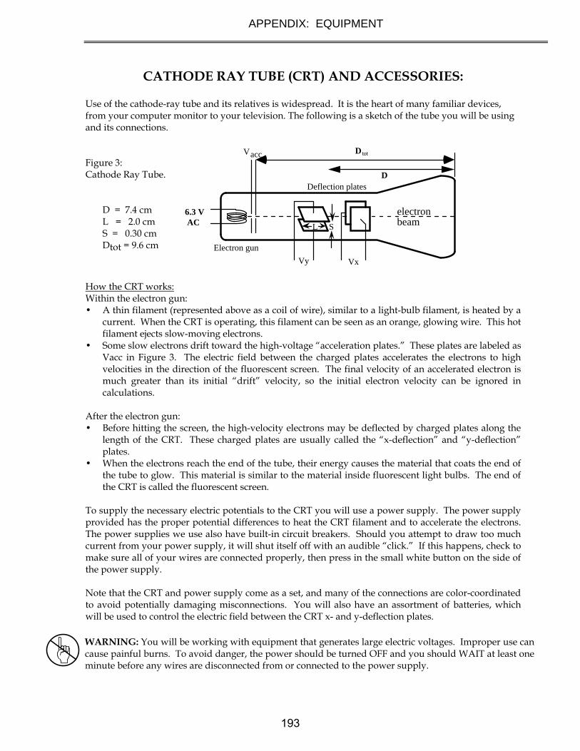
APPENDIX: EQUIPMENT
CATHODE RAY TUBE (CRT) AND ACCESSORIES:
Use of the cathode-ray tube and its relatives is widespread. It is the heart of many familiar devices, from your computer monitor to your television. The following is a sketch of the tube you will be using and its connections. Figure 3: Cathode Ray Tube.
D = 7.4 cm L = 2.0 cm S = 0.30 cm Dtot = 9.6 cm
How the CRT works: Within the electron gun: • A thin filament (represented above as a coil of wire), similar to a light-bulb filament, is heated by a
current. When the CRT is operating, this filament can be seen as an orange, glowing wire. This hot filament ejects slow-moving electrons.
• Some slow electrons drift toward the high-voltage “acceleration plates.” These plates are labeled as Vacc in Figure 3. The electric field between the charged plates accelerates the electrons to high velocities in the direction of the fluorescent screen. The final velocity of an accelerated electron is much greater than its initial “drift” velocity, so the initial electron velocity can be ignored in calculations.
After the electron gun: • Before hitting the screen, the high-velocity electrons may be deflected by charged plates along the
length of the CRT. These charged plates are usually called the “x-deflection” and “y-deflection” plates.
• When the electrons reach the end of the tube, their energy causes the material that coats the end of the tube to glow. This material is similar to the material inside fluorescent light bulbs. The end of the CRT is called the fluorescent screen.
To supply the necessary electric potentials to the CRT you will use a power supply. The power supply provided has the proper potential differences to heat the CRT filament and to accelerate the electrons. The power supplies we use also have built-in circuit breakers. Should you attempt to draw too much current from your power supply, it will shut itself off with an audible “click.” If this happens, check to make sure all of your wires are connected properly, then press in the small white button on the side of the power supply. Note that the CRT and power supply come as a set, and many of the connections are color-coordinated to avoid potentially damaging misconnections. You will also have an assortment of batteries, which will be used to control the electric field between the CRT x- and y-deflection plates.
WARNING: You will be working with equipment that generates large electric voltages. Improper use can cause painful burns. To avoid danger, the power should be turned OFF and you should WAIT at least one minute before any wires are disconnected from or connected to the power supply.
6.3 V AC
Vy
D
S
Vx
L
electron beam
Electron gun
totDVacc
Deflection plates
193

APPENDIX: EQUIPMENT
To properly connect the CRT to the power supply: 1. Turn the power supply off. 2. Connect the power supply ports marked “AC 6.3V” (they are green; the voltage differs slightly
from one supply to another, but should be clearly marked) to the ports marked “HEATER” or “FILAMENT” on the CRT (these are also green).
3. Connect the appropriate accelerating potential across the cathode and anode. For instance, if your experiment calls for a 500 volt accelerating potential, connect the cathode to the port marked “–250 V” (which may be black or white) and the anode to the port marked “+ 250 V” (which is red). This gives a total potential difference of 500 volts.
4. Turn the power supply on.
194

APPENDIX: EQUIPMENT
RESISTOR CODES
A resistor is a circuit element manufactured to have a constant resistance. The resistance is coded onto the side of the resistor in colored bands, where the color and position of the bands tell you what the resistance is.
To read the color bands on the resistor, begin by finding the gold or silver band on one end of the resistor; this is the back of the resistor. You begin reading from the other end. Most resistors (including those you will use in lab) are coded to two significant digits. The first two color bands correspond to these two significant digits. The third color band is called the multiplier. The number coded by this band represents a power of ten which you multiply by the number from the first two bands to get the total resistance. The fourth color band tells you the tolerance, or error bounds for the coded resistance: gold means ±5% tolerance, silver means ±10% tolerance and no fourth band means ±20%. Some resistors have a fifth color band, which represents the reliability of the resistor, and can just be ignored for the purposes of these labs.
Examples:
%201010 2 R %51056 4 R
Color Number Black
Brown Red
Orange Yellow Green Blue
Violet Gray White
0 1 2 3 4 5 6 7 8 9
195

APPENDIX: EQUIPMENT
POWER SUPPLIES
The 18volt 5 amp power supply is an all-purpose power supply for the production of constant currents and voltages. At the top is the main display that reads either current in Amperes or voltage in Volts. There is a switch there that allows you to switch between them. The current and voltage controls are located in the middle. In between the constant current and constant voltage knobs is a switch that allows you to toggle from high currents to low currents. It is highly recommended that you use only the low current mode.
This power supply normally operates in the constant voltage mode. As such, you can only change the voltages by using the constant voltage knobs. In the event that too much is being pulled from the power supply (as in a short), it will automatically switch to the constant current mode, where the amount of current flowing is greatly reduced. This is a signal that something is amiss with your circuit. There is a mater-slave switch on the back of the power supply. This should always be set to master for the DMM to function properly. If you experience any problems, this is the first place to check.
196
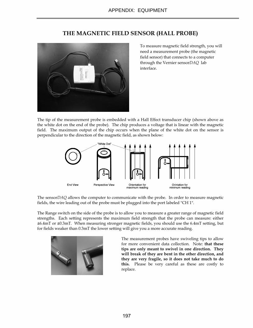
APPENDIX: EQUIPMENT
THE MAGNETIC FIELD SENSOR (HALL PROBE)
To measure magnetic field strength, you will
need a measurement probe (the magnetic
field sensor) that connects to a computer
through the Vernier sensorDAQ lab
interface.
The tip of the measurement probe is embedded with a Hall Effect transducer chip (shown above as the white dot on the end of the probe). The chip produces a voltage that is linear with the magnetic field. The maximum output of the chip occurs when the plane of the white dot on the sensor is perpendicular to the direction of the magnetic field, as shown below:
The sensorDAQ allows the computer to communicate with the probe. In order to measure magnetic fields, the wire leading out of the probe must be plugged into the port labeled "CH 1". The Range switch on the side of the probe is to allow you to measure a greater range of magnetic field strengths. Each setting represents the maximum field strength that the probe can measure: either ±6.4mT or ±0.3mT. When measuring stronger magnetic fields, you should use the 6.4mT setting, but for fields weaker than 0.3mT the lower setting will give you a more accurate reading.
The measurement probes have swiveling tips to allow for more convenient data collection. Note: that these tips are only meant to swivel in one direction. They will break of they are bent in the other direction, and they are very fragile, so it does not take much to do this. Please be very careful as these are costly to replace.
197

APPENDIX: EQUIPMENT
RE-MAGNETIZING A BAR MAGNET The magnetizer should be used if you have a bad bar magnet that isn’t a simple dipole, polarity doesn’t match the labels, or the magnet is too weak.
Important to know is that the magnetizer is poorly labeled. The N and S do not indicate the end of the magnet that goes into the magnetizer! We believe the company is trying to imply that magnets inserted into the side labeled N will be north attracting and vice versa. You need to insert the S pole of the bar magnet into the side labeled N and the N pole of the bar magnet into the side labeled S.
198

Appendix: SOFTWARE
MAGNETLAB - MEASURING CONSTANT MAGNETIC FIELD Application Basics Before you begin, you should ensure that you have read the relevant sections of Appendix A to familiarize yourself with the equipment. The software package that works in tandem with your magnetic field sensor is written in LabVIEW™. It allows you to measure and record magnetic field strength as a function of a number of different variables. After logging into the computer, execute the application by double clicking the “MAGNETLAB” icon located in the PhysLab folder on the desktop. Before you start using the program, you should take a moment to identify several key elements. The two most important of these are the Command Panel, shown to the right, and the Guide Box, shown below.
The Guide Box will give you directions and tasks to perform. It will also tell you when to select a command in the Command Panel. After selecting a command, it will “gray out” and the next command will become available. You can also print and/or quit from the Command Panel or abort your analysis and try again.
The primary data output you get is by generating pdf files of your results, so be careful not to quit without printing pdf files or exporting your data to be emailed amongst your lab group.
199

APPENDIX: SOFTWARE
Calibration The first command is to calibrate the Magnetic Field Sensor. Before selecting this command, you need to set the probe to the 6.4mT setting.
After selecting the "Calibrate Probe" command, you will be asked to do two tasks. First, you will need to choose the quantity on the x-axis of your data graph. This is accomplished by moving the cursor over to the word "meter" in the red-colored area (shown below) and then pressing the mouse button.
You should get a list of choices as shown to the right. By selecting any of these units, you will be making a choice about what you wish to measure. For example, if you choose to use "cm”, you will make a graph of magnetic field strength as a function of distance (B vs. x). It is likely you will want to choose a small unit (cm’s or mm’s) to measure the distance in, since many magnetic fields are not very strong over long distances Selecting "degree" will make a plot of magnetic field strength as a function of angle (B vs. ). Click "OK" when you are ready to proceed.
Second, you will need to eliminate the effect of the background magnetic fields. This process is called "zeroing the Hall probe" in the Guide Box. Place the magnetic field sensor wand in the position you would like to take your measurement, but be sure that there are no magnets nearby. Note that power supplies and computers generate magnetic fields, so it is a good idea to keep away from them! When you are ready, select the "Set Probe Zero" as shown below. Then select the “Done” button. The calibration process is now complete. Predictions This type of analysis relies on your graphical skills to interpret the data. You should be familiar with both appendices, A Review of Graphs and Accuracy, Precision and Uncertainty.
The first task is to enter your prediction of the mathematical function you expect to represent your data. Making a prediction before taking data is the best way to determine if anything is going wrong (remember Murphy’s Law). It’s also a good way to make sure you have learned
200

APPENDIX: SOFTWARE
something, but only if you stop to think about the discrepancies or similarities between your prediction and the results. In order to enter your prediction, you first need to decide on your coordinate axes and scale (units) for your measurements. Record these in your lab journal. Next, you will need to select the generic equation, u(x), which describes the graph you expect for the data. Clicking the equation currently showing in the box will bring up a list of equations to choose from; see the diagrams to the right. After selecting your generic equation, you need to enter your best approximation for the parameters A, B, C, and/or D. These values should come directly from your prediction equation you did for class. As you enter these values, you should see the red line in the "Plot" box changing.
Once you have selected an equation and the values of the constants are entered, your prediction equation is shown on the graph on the computer screen. If you do not see the curve representing your prediction, change the scale of the graph axes or use the AutoScale feature (see Finding Data below). When you are satisfied, select the Accept Prediction option from the Command Panel. Once you have done this you cannot change your prediction except by starting over. Exploration After you have entered your prediction, you can explore the limitations of your magnetic field sensor before you take data. The value of the magnetic field strength is displayed directly under the Guide Box. When you are ready to take data, select Acquire Data from the Command Panel. Data Acquisition Collecting data requires that you enter the x-axis data before the computer reads in a value for the magnetic field strength. You enter this data using the panel shown. For every x-axis data value you enter, the analysis program will record the magnetic field strength in gauss on the y-axis of the "Plot". Press "OK" to collect the next data point.
201

APPENDIX: SOFTWARE
Each data point should appear on the graph on the computer screen as you take it. If it doesn’t, adjust the scales of your graph axes or use the AutoScale feature (see Finding Data below). If you are satisfied with your data, choose Analyze Data from the Command Panel.
Finding Data on the Graph You can find your data on the graph by adjusting the scales of your X-axis and Y-axis plots manually. This scaling is accomplished by entering values into the legend of the graph. Click on the upper or lower legend value and enter a new value, then hit enter. If you cannot locate your data, you can select both "AutoScale Y-axis" and "AutoScale X-Axis" to let the program find the data for you. You can then adjust your axis scales to give you a convenient graph for analysis. Be careful, the AutoScale option will often set the scales in such a way that small fluctuations in the data are magnified into huge fluctuations.
Data Fits Deciding which equation best fits your data is the most important part of using this analysis program. While the actual mechanics of choosing the equation and parameter is similar to what you did for your predictions, fitting data is somewhat more complicated. By looking at the behavior of the data on the graph, determine the best possible function to describe this data. After you have decided on the appropriate equation, you need to determine the constants of this equation so that it best fits the data. Although this can be done by trial and error, it is much more efficient to think of how the behavior of the equation you have chosen depends on each parameter. Calculus can be a great help here. This can be a time-consuming task, so be patient.
Now you need to estimate the uncertainty in your fit by deciding the range of other lines that could also fit your data. This method of estimating your uncertainty is described in Appendix D. Slightly changing the values for each constant in turn will allow you to do this quickly.
After you have computed your uncertainties, return to your best-fit line and use it as your fit by selecting Accept Fit in the Command Panel. Importing / Exporting Data After you have selected Analyze Data, it is possible to save your data to the computer's hard drive. This feature can come in handy if you need to analyze your data at a later date or if you want to re-analyze your data after you have printed it out.
To save your data, simply select Export Data and follow the instructions in the windows. Your file should be saved in the LabData folder. To retrieve this file, restart MagnetLab from the desktop and select Import Data.
202

APPENDIX: SOFTWARE
Last Words
These directions are not meant to be exhaustive. You will discover more features as you analyze more data. Be sure to record these features in your lab journal.
203
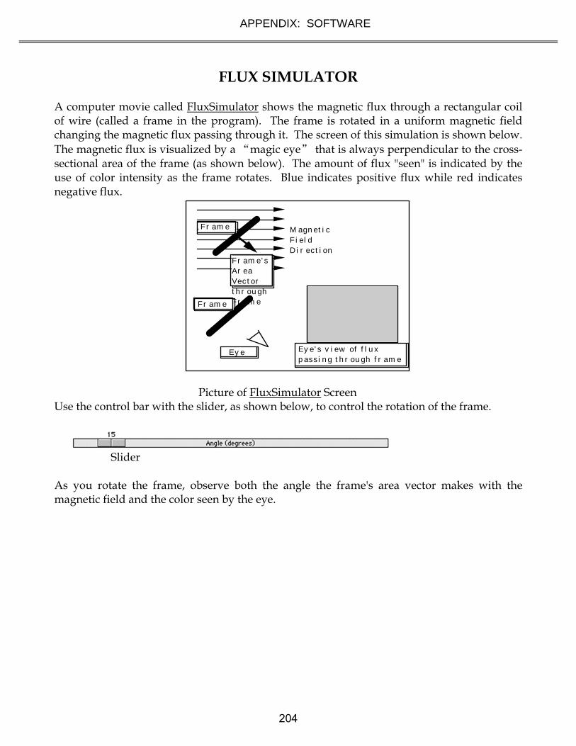
APPENDIX: SOFTWARE
FLUX SIMULATOR
A computer movie called FluxSimulator shows the magnetic flux through a rectangular coil of wire (called a frame in the program). The frame is rotated in a uniform magnetic field changing the magnetic flux passing through it. The screen of this simulation is shown below. The magnetic flux is visualized by a “magic eye” that is always perpendicular to the cross-sectional area of the frame (as shown below). The amount of flux "seen" is indicated by the use of color intensity as the frame rotates. Blue indicates positive flux while red indicates negative flux.
Fr am e' sAr eaVect ort h r ou ghFr am e
M agn et i cF i el dDi r ect i on
Fr am e
Ey e
Fr am e
Ey e' s v i ew of f l u xp assi n g t h r ou gh f r am e
Picture of FluxSimulator Screen Use the control bar with the slider, as shown below, to control the rotation of the frame.
Slider
As you rotate the frame, observe both the angle the frame's area vector makes with the magnetic field and the color seen by the eye.
204

APPENDIX: SOFTWARE
VoltageTimeLAB - MEASURING TIME-VARYING VOLTAGES The Basics: This software package, written in LabVIEW™, allows you to measure and record potential differences as a function of time. The software and voltage interface act much like an oscilloscope. After logging into the computer, execute the application by double clicking the “VoltageTimeLab” icon located in the PhysLab folder on the desktop. Before you start using the program, you should take a moment to identify several key elements. The two most important of these are the Command Panel, shown to the right, and the Guide Box, shown below.
The Guide Box will give you directions and tasks to perform. It will also tell you when to select a command in the Command Panel. You can also print and/or quit from the Command Panel or abort your analysis and try again.
The primary data output you get is by generating pdf files of your results, so be careful not to quit without printing pdf files or exporting your data.
Since the application to measure time-varying voltage is a slight modification of the application to measure magnetic field, you are already familiar with how to use much of it. The basic difference between the TimeVoltageLab and the MagnetLab applications is an additional display that is much like an oscilloscope. The potential difference versus time display is shown on the next page. The DAQ (Data Acquisition) control buttons are located directly above this display. The “DAQ START” and “DAQ STOP” buttons do as they suggest, stop and start data streaming from the probe to the voltage versus time display. When you first start the application you will need to click the “DAQ START” button to start
205
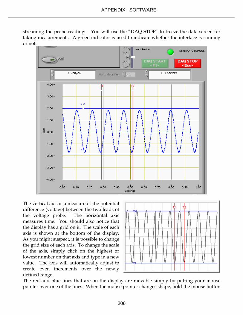
APPENDIX: SOFTWARE
streaming the probe readings. You will use the “DAQ STOP” to freeze the data screen for taking measurements. A green indicator is used to indicate whether the interface is running or not.
The vertical axis is a measure of the potential difference (voltage) between the two leads of the voltage probe. The horizontal axis measures time. You should also notice that the display has a grid on it. The scale of each axis is shown at the bottom of the display. As you might suspect, it is possible to change the grid size of each axis. To change the scale of the axis, simply click on the highest or lowest number on that axis and type in a new value. The axis will automatically adjust to create even increments over the newly defined range.
The red and blue lines that are on the display are movable simply by putting your mouse pointer over one of the lines. When the mouse pointer changes shape, hold the mouse button
206

APPENDIX: SOFTWARE
down and drag the lines to mark a voltage or time as shown. The lines mark the voltage and time boundaries of the data that will be considered for analysis.
If you are unable to see the lines, it is possible that you changed the axes scale and “zoomed in” too far. Try changing the axes to “zoom out” again, and determine if you can locate the blue and red lines. Move the lines to within the values of the new scale, and they should remain visible on the screen when you zoom in. Predictions This type of analysis relies on your graphical skills to interpret the data. You should be familiar with both appendices, A Review of Graphs and Accuracy, Precision and Uncertainty. The first task is to enter your prediction of the mathematical function you expect to represent your data. Making a prediction before taking data is the best way to determine if anything is going wrong (remember Murphy’s Law). It’s also a good way to make sure you have learned something, but only if you stop to think about the discrepancies or similarities between your prediction and the results. You will need to select the generic equation, u(x), which describes the graph you expect for the data. Clicking the equation currently showing in the box will bring up a list of equations to choose from; see the diagrams to the right. After selecting your generic equation, you next need to enter your best approximation for the parameters A, B, C, and/or D. These values should come directly from your prediction equation you did for class. As you enter these values, you should see the red line in the "Plot" box changing.
Once you have selected an equation and the values of the constants are entered, your prediction equation is shown on the graph on the computer screen. If you do not see the curve representing your prediction, change the scale of the graph axes (see Finding Data below). When you are satisfied, select the Accept Prediction option from the Command Panel. Once you have done this you cannot change your prediction except by starting over.
207

APPENDIX: SOFTWARE
Exploration After you have entered your prediction, you can explore the limitations of your voltage probe sensor before you take data. The value of the voltage is displayed directly on the voltage vs. time display. When you are ready to take data, select Acquire Data from the Command Panel. Data Acquisition Collecting data requires that you position the moveable red and blue lines on the voltage vs. time display. The blue lines will generate potential difference data and the red lines will generate time/period data. The data values are shown in the data box. The data box appears once you have selected “Acquire Data” from the Command Panel. Press "OK" to collect each data point. Each data point should appear on the graph on the computer screen as you take it. If it doesn’t, adjust the scales of your graph axes. If you are satisfied with your data, choose Analyze Data from the Command Panel.
Finding Data on the Graph You can find your data on the graph by adjusting the scales of your X-axis and Y-axis plots manually. This scaling is accomplished by entering values into the legend of the graph. Click on the upper or lower legend value and enter a new value, then hit enter. If you cannot locate your data, you can select both "AutoScale Y-axis" and "AutoScale X-Axis" to let the program find the data for you. You can then adjust your axis scales to give you a convenient graph for analysis. Be careful, the AutoScale option will often set the scales in such a way that small fluctuations in the data are magnified into huge fluctuations.
Data Fits Deciding which equation best fits your data is the most important part of using this analysis program. While the actual mechanics of choosing the equation and parameters are similar to what you did for your predictions, fitting data is somewhat more complicated. By looking at the behavior of the data on the graph, determine the best possible function to describe this data. After you have decided on the appropriate equation, you need to determine the constants of this equation so that it best fits the data. Although this can be done by trial and error, it is much more efficient to think of how the behavior of the equation
208

APPENDIX: SOFTWARE
you have chosen depends on each parameter. Calculus can be a great help here. This can be a time-consuming task, so be patient.
Now you need to estimate the uncertainty in your fit by deciding the range of other lines that could also fit your data. This method of estimating your uncertainty is described in the appendix Accuracy, Precision and Uncertainty. Slightly changing the values for each constant in turn will allow you to do this quickly.
After you have computed your uncertainties, return to your best-fit line and use it as your fit by selecting Accept Fit in the Command Panel.
209

APPENDIX: SOFTWARE
Excel - MAKING GRAPHS
You will find that numerous exercises in this manual will require graphs. Microsoft Excel is a spreadsheet program that can create fourteen types of graphs, each of which have from two to ten different formats. This results in a maze of possibilities. There are help screens in Excel; however, this overview is covers the type of graph you should include in your lab reports. This is meant to be a brief introduction to the use of Microsoft Excel for graphing scientific data. If you are acquainted with Excel already, you should still skim through this appendix to learn about the type of graph to include in reports. Step 1. Input your measurements and highlight the data using your cursor.
210

APPENDIX: SOFTWARE
Step 2. Click on the “Chart Wizard” on the toolbar.
Step 3. Choose XY Scatter, not Line, from the list and click the “Next” button.
211

APPENDIX: SOFTWARE
Step 4. Select the “Series in: Columns” option and click the “Next” button.
Step 5. Fill in the chart title and axis labels, and click the “Next” button.
212
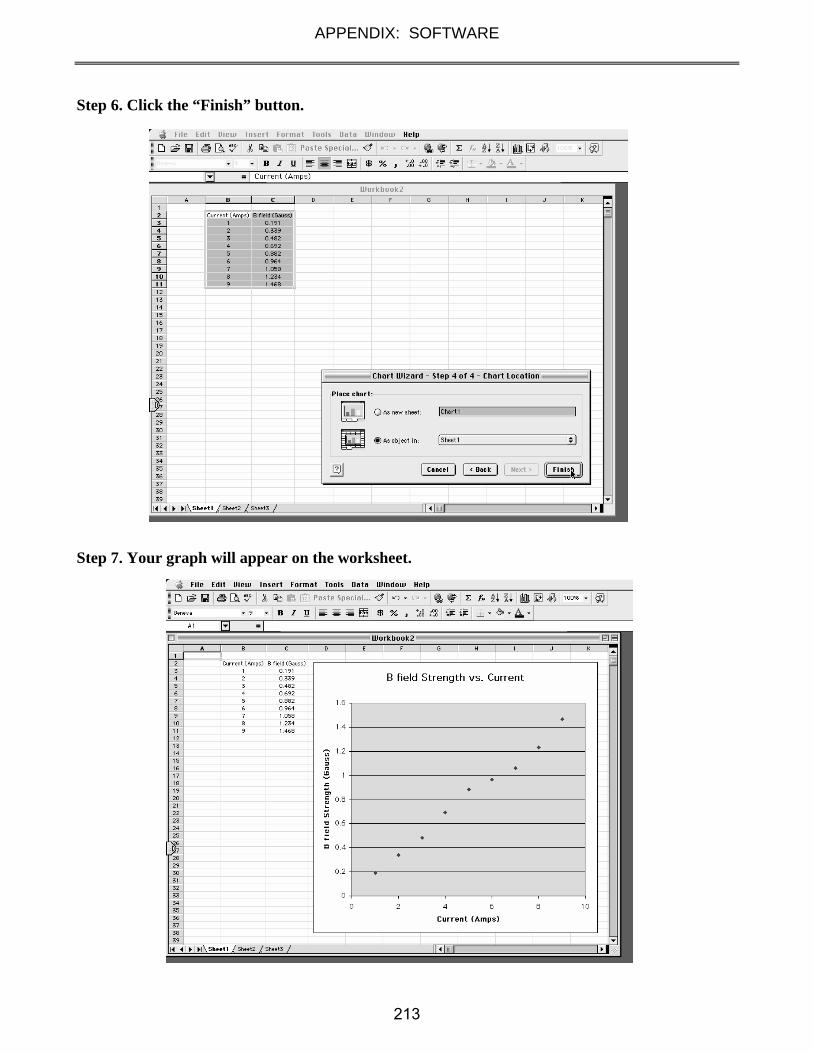
APPENDIX: SOFTWARE
Step 6. Click the “Finish” button.
Step 7. Your graph will appear on the worksheet.
213

APPENDIX: SOFTWARE
Step 8. Click on the data points to highlight them.
Step 9. Select “Add a Trendline” from the “Chart” menu.
214
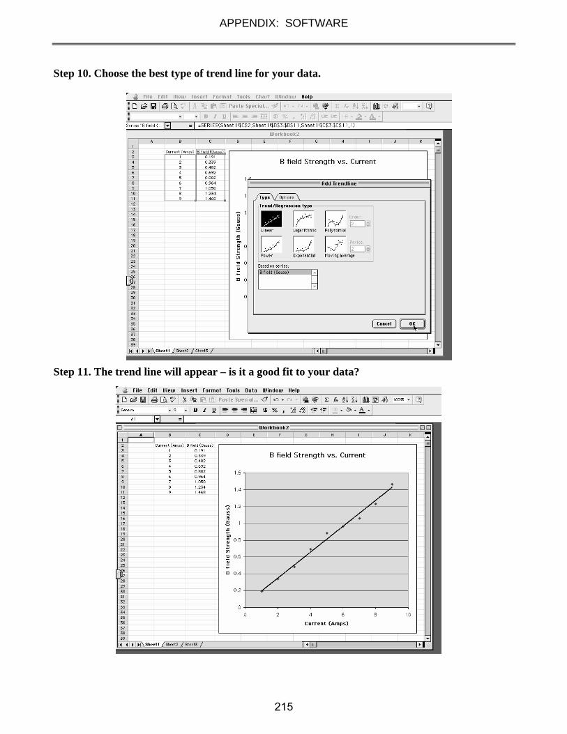
APPENDIX: SOFTWARE
Step 10. Choose the best type of trend line for your data.
Step 11. The trend line will appear – is it a good fit to your data?
215

APPENDIX: SOFTWARE
Step 12. If the equation of the line is needed, choose “Display equation on chart.”
Step 13. The equation of the trend line should appear on your graph.
216

Appendix: Significant Figures
Calculators make it possible to get an answer with a huge number of figures. Unfortunately, many of them are meaningless. For instance, if you needed to split $1.00 among three people, you could
never give them each exactly $0.333333 … The same is true for measurements. If you use a meter stick with millimeter markings to measure the length of a key, as in Figure 1, you could not measure more precisely than a quarter or half or a third of a mm. Reporting a number like 5.37142712 cm would not only be meaningless, it would be misleading.
Figure 1
In your measurement, you can precisely determine the distance down to the nearest millimeter and then improve your precision by estimating the next figure. It is always assumed that the last figure in the number recorded is uncertain. So, you would report the length of the key as 5.37 cm. Since you estimated the 7, it is the uncertain figure. If you don't like estimating, you might be tempted to just give the number that you know best, namely 5.3 cm, but it is clear that 5.37 cm is a better report of the measurement. An estimate is always necessary to report the most precise measurement. When you quote a measurement, the reader will always assume that the last figure is an estimate. Quantifying that estimate is known as estimating uncertainties. Appendix C will illustrate how you might use those estimates
to determine the uncertainties in your measurements.
What are significant figures? The number of significant figures tells the reader the precision of a measurement. Table 1 gives some examples. Table 1
Length (centimeters)
Number of Significant Figures
12.74 4
11.5 3
1.50 3
1.5 2
12.25345 7
0.8 1
0.05 1
One of the things that this table illustrates is that not all zeros are significant. For example, the zero in 0.8 is not significant, while the zero in 1.50 is significant. Only the zeros that appear after the first non-zero digit are significant. A good rule is to always express your values in scientific notation. If you say that your friend lives 143 m from you, you are saying that you are sure of that distance to within a few meters (3 significant figures). What if you really only know the distance to a few tens of meters (2 significant figures)? Then you need to express the distance in scientific notation 1.4 x 10² m.
Is it always better to have more figures? Consider the measurement of the length of the key shown in Figure 1. If we have a scale with ten etchings to every millimeter, we could use a microscope to measure the spacing to the nearest tenth of a millimeter
217

APPENDIX: SIGNIFICANT FIGURES
and guess at the one hundredth millimeter. Our measurement could be 5.814 cm with the uncertainty in the last figure, four significant figures instead of three. This is because our improved scale allowed our estimate to be more precise. This added precision is shown by more significant figures. The more significant figures a number has, the more precise it is.
How do I use significant figures in calculations? When using significant figures in calculations, you need to keep track of how the uncertainty propagates. There are mathematical procedures for doing this estimate in the most precise manner. This type of estimate depends on knowing the statistical distribution of your measurements. With a lot less effort, you can do a cruder estimate of the uncertainties in a calculated result. This crude method gives an overestimate of the uncertainty but it is a good place to start. For this course this simplified uncertainty estimate (described in Appendix C and below) will be good enough.
Addition and subtraction When adding or subtracting numbers, the number of decimal places must be taken into account. The result should be given to as many decimal places as the term in the sum that is given to the smallest number of decimal places. Examples:
Addition Subtraction
6.242 5.875 +4.23 -3.34 +0.013 2.535
10.485
10.49 2.54
The uncertain figures in each number are shown in bold-faced type.
Multiplication and division When multiplying or dividing numbers, the number of significant figures must be taken into account. The result should be given to as many significant figures as the term in the product that is given to the smallest number of significant figures. The basis behind this rule is that the least accurately known term in the product will dominate the accuracy of the answer. As shown in the examples, this does not always work, though it is the quickest and best rule to use. When in doubt, you can keep track of the significant figures in the calculation as is done in the examples.
Examples:
Multiplication
15.84 17.27 x 2.5 x 4.0 7920 69.080
3168 39.600
40 69
Division
117 25 23)2691 75)1875
23 150 39 375 23 375 161 161
1.2 x 10² 2.5 x 101
218

APPENDIX: SIGNIFICANT FIGURES
PRACTICE EXERCISES 1. Determine the number of significant figures of the quantities in the following
table:
Length (centimeters)
Number of Significant
Figures
17.87
0.4730
17.9
0.473
18
0.47
1.34 x 10²
2.567x 10⁵
2.0 x 10¹⁰
1.001
1.000
1
1000
1001
2. Add: 121.3 to 6.7 x 10²: [Answer: 121.3 + 6.7 x 102 = 7.9 x 10²]
3. Multiply: 34.2 and 1.5 x 10⁴
[Answer: 34.2 x 1.5 x 104 = 5.1 x 10⁵]
219

APPENDIX: SIGNIFICANT FIGURES
220
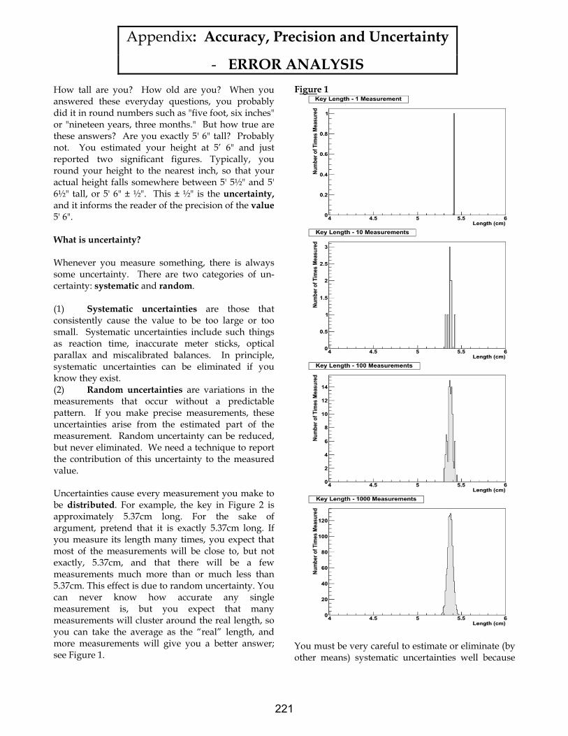
Appendix: Accuracy, Precision and Uncertainty
- ERROR ANALYSIS
How tall are you? How old are you? When you answered these everyday questions, you probably did it in round numbers such as "five foot, six inches" or "nineteen years, three months." But how true are these answers? Are you exactly 5' 6" tall? Probably not. You estimated your height at 5’ 6" and just reported two significant figures. Typically, you round your height to the nearest inch, so that your actual height falls somewhere between 5' 5½" and 5' 6½" tall, or 5' 6" ± ½". This ± ½" is the uncertainty, and it informs the reader of the precision of the value 5' 6". What is uncertainty? Whenever you measure something, there is always some uncertainty. There are two categories of un-certainty: systematic and random. (1) Systematic uncertainties are those that consistently cause the value to be too large or too small. Systematic uncertainties include such things as reaction time, inaccurate meter sticks, optical parallax and miscalibrated balances. In principle, systematic uncertainties can be eliminated if you know they exist. (2) Random uncertainties are variations in the measurements that occur without a predictable pattern. If you make precise measurements, these uncertainties arise from the estimated part of the measurement. Random uncertainty can be reduced, but never eliminated. We need a technique to report the contribution of this uncertainty to the measured value. Uncertainties cause every measurement you make to be distributed. For example, the key in Figure 2 is approximately 5.37cm long. For the sake of argument, pretend that it is exactly 5.37cm long. If you measure its length many times, you expect that most of the measurements will be close to, but not exactly, 5.37cm, and that there will be a few measurements much more than or much less than 5.37cm. This effect is due to random uncertainty. You can never know how accurate any single measurement is, but you expect that many measurements will cluster around the real length, so you can take the average as the “real” length, and more measurements will give you a better answer; see Figure 1.
Figure 1
You must be very careful to estimate or eliminate (by other means) systematic uncertainties well because
221

APPENDIX: ACCURACY, PRECISION AND UNCERTAINTY
they cannot be eliminated in this way; they would just shift the distributions in Figure 1 left or right. Roughly speaking, the average or “center” of the distribution is the “measurement,” and the width or “deviation” of the distribution is the random uncertainty. How do I determine the uncertainty? This Appendix will discuss three basic techniques for determining the uncertainty: estimating the uncertainty, measuring the average deviation, and finding the uncertainty in a linear fit. Which one you choose will depend on your situation, your available means of measurement, and your need for precision. If you need a precise determination of some value, and you are measuring it directly (e.g., with a ruler or thermometer), the best technique is to measure that value several times and use the average deviation as the uncertainty. Examples of finding the average deviation are given below. How do I estimate uncertainties? If time or experimental constraints make repeated measurements impossible, then you will need to estimate the uncertainty. When you estimate uncertainties you are trying to account for anything that might cause the measured value to be different if you were to take the measurement again. For example, suppose you were trying to measure the length of a key, as in Figure 2. Figure 2
If the true value were not as important as the magnitude of the value, you could say that the key’s length was 5cm, give or take 1cm. This is a crude estimate, but it may be acceptable. A better estimate of the key’s length, as you saw in Appendix A, would be 5.37cm. This tells us that the worst our
measurement could be off is a fraction of a mm. To be more precise, we can estimate it to be about a third of a mm, so we can say that the length of the key is 5.37 ± 0.03 cm. Another time you may need to estimate uncertainty is when you analyze video data. Figures 3 and 4 show a ball rolling off the edge of a table. These are two consecutive frames, separated in time by 1/30 of a second. Figure 3
Figure 4
The exact moment the ball left the table lies somewhere between these frames. We can estimate that this moment occurs midway between them (
). Since it must occur at some point
between them, the worst our estimate could be off by
st 60110
222
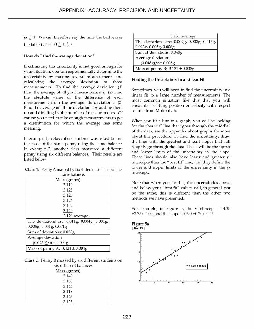
APPENDIX: ACCURACY, PRECISION AND UNCERTAINTY
is . We can therefore say the time the ball leaves
the table is
How do I find the average deviation? If estimating the uncertainty is not good enough for your situation, you can experimentally determine the un-certainty by making several measurements and calculating the average deviation of those measurements. To find the average deviation: (1) Find the average of all your measurements; (2) Find the absolute value of the difference of each measurement from the average (its deviation); (3) Find the average of all the deviations by adding them up and dividing by the number of measurements. Of course you need to take enough measurements to get a distribution for which the average has some meaning. In example 1, a class of six students was asked to find the mass of the same penny using the same balance. In example 2, another class measured a different penny using six different balances. Their results are listed below:
Class 1: Penny A massed by six different students on the
same balance. Mass (grams)
3.110 3.125 3.120 3.126 3.122 3.120
3.121 average. The deviations are: 0.011g, 0.004g, 0.001g, 0.005g, 0.001g, 0.001g Sum of deviations: 0.023g Average deviation: (0.023g)/6 = 0.004g Mass of penny A: 3.121 ± 0.004g
Class 2: Penny B massed by six different students on
six different balances Mass (grams)
3.140 3.133 3.144 3.118 3.126 3.125
3.131 average The deviations are: 0.009g, 0.002g, 0.013g, 0.013g, 0.005g, 0.006g Sum of deviations: 0.048g Average deviation: (0.048g)/6= 0.008g Mass of penny B: 3.131 ± 0.008g
Finding the Uncertainty in a Linear Fit Sometimes, you will need to find the uncertainty in a linear fit to a large number of measurements. The most common situation like this that you will encounter is fitting position or velocity with respect to time from MotionLab. When you fit a line to a graph, you will be looking for the “best fit” line that “goes through the middle” of the data; see the appendix about graphs for more about this procedure. To find the uncertainty, draw the lines with the greatest and least slopes that still roughly go through the data. These will be the upper and lower limits of the uncertainty in the slope. These lines should also have lesser and greater y-intercepts than the “best fit” line, and they define the lower and upper limits of the uncertainty in the y-intercept. Note that when you do this, the uncertainties above and below your “best fit” values will, in general, not be the same; this is different than the other two methods we have presented. For example, in Figure 5, the y-intercept is 4.25 +2.75/-2.00, and the slope is 0.90 +0.20/-0.25. Figure 5a
s601
.10 601
601 st
223
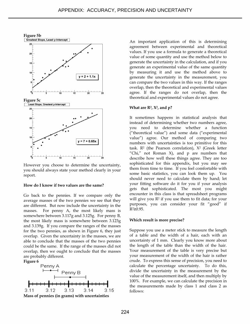
APPENDIX: ACCURACY, PRECISION AND UNCERTAINTY
Figure 5b
Figure 5c
However you choose to determine the uncertainty, you should always state your method clearly in your report. How do I know if two values are the same? Go back to the pennies. If we compare only the average masses of the two pennies we see that they are different. But now include the uncertainty in the masses. For penny A, the most likely mass is somewhere between 3.117g and 3.125g. For penny B, the most likely mass is somewhere between 3.123g and 3.139g. If you compare the ranges of the masses for the two pennies, as shown in Figure 6, they just overlap. Given the uncertainty in the masses, we are able to conclude that the masses of the two pennies could be the same. If the range of the masses did not overlap, then we ought to conclude that the masses are probably different. Figure 6
Mass of pennies (in grams) with uncertainties
An important application of this is determining agreement between experimental and theoretical values. If you use a formula to generate a theoretical value of some quantity and use the method below to generate the uncertainty in the calculation, and if you generate an experimental value of the same quantity by measuring it and use the method above to generate the uncertainty in the measurement, you can compare the two values in this way. If the ranges overlap, then the theoretical and experimental values agree. If the ranges do not overlap, then the theoretical and experimental values do not agree. What are R2, X2, and p? It sometimes happens in statistical analysis that instead of determining whether two numbers agree, you need to determine whether a function (“theoretical value”) and some data (“experimental value”) agree. Our method of comparing two numbers with uncertainties is too primitive for this task. R2 (the Pearson correlation), X2 (Greek letter “Chi,” not Roman X), and p are numbers that describe how well these things agree. They are too sophisticated for this appendix, but you may see them from time to time. If you feel comfortable with some basic statistics, you can look them up. You should never need to calculate them by hand; let your fitting software do it for you if your analysis gets that sophisticated. The most you might encounter in this class is that spreadsheet programs will give you R2 if you use them to fit data; for your purposes, you can consider your fit “good” if R2≥0.95. Which result is more precise? Suppose you use a meter stick to measure the length of a table and the width of a hair, each with an uncertainty of 1 mm. Clearly you know more about the length of the table than the width of the hair. Your measurement of the table is very precise but your measurement of the width of the hair is rather crude. To express this sense of precision, you need to calculate the percentage uncertainty. To do this, divide the uncertainty in the measurement by the value of the measurement itself, and then multiply by 100%. For example, we can calculate the precision in the measurements made by class 1 and class 2 as follows:
224
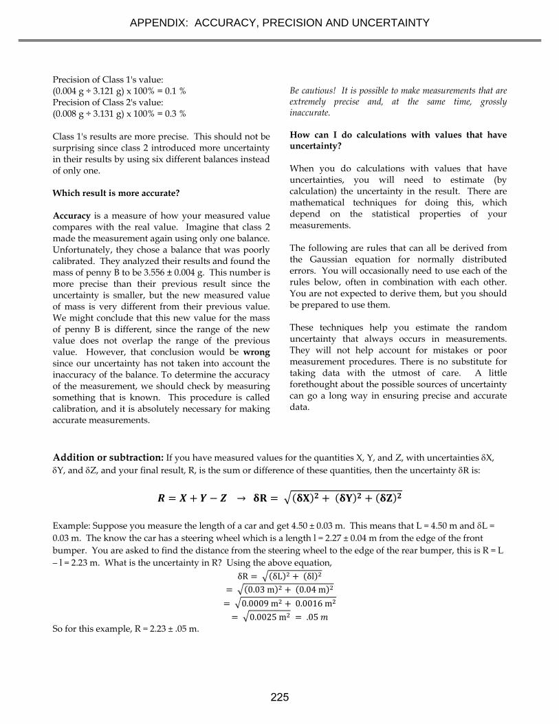
APPENDIX: ACCURACY, PRECISION AND UNCERTAINTY
Precision of Class 1's value: (0.004 g ÷ 3.121 g) x 100% = 0.1 % Precision of Class 2's value: (0.008 g ÷ 3.131 g) x 100% = 0.3 % Class 1's results are more precise. This should not be surprising since class 2 introduced more uncertainty in their results by using six different balances instead of only one. Which result is more accurate? Accuracy is a measure of how your measured value compares with the real value. Imagine that class 2 made the measurement again using only one balance. Unfortunately, they chose a balance that was poorly calibrated. They analyzed their results and found the mass of penny B to be 3.556 ± 0.004 g. This number is more precise than their previous result since the uncertainty is smaller, but the new measured value of mass is very different from their previous value. We might conclude that this new value for the mass of penny B is different, since the range of the new value does not overlap the range of the previous value. However, that conclusion would be wrong since our uncertainty has not taken into account the inaccuracy of the balance. To determine the accuracy of the measurement, we should check by measuring something that is known. This procedure is called calibration, and it is absolutely necessary for making accurate measurements.
Be cautious! It is possible to make measurements that are extremely precise and, at the same time, grossly inaccurate. How can I do calculations with values that have uncertainty? When you do calculations with values that have uncertainties, you will need to estimate (by calculation) the uncertainty in the result. There are mathematical techniques for doing this, which depend on the statistical properties of your measurements. The following are rules that can all be derived from the Gaussian equation for normally distributed errors. You will occasionally need to use each of the rules below, often in combination with each other. You are not expected to derive them, but you should be prepared to use them. These techniques help you estimate the random uncertainty that always occurs in measurements. They will not help account for mistakes or poor measurement procedures. There is no substitute for taking data with the utmost of care. A little forethought about the possible sources of uncertainty can go a long way in ensuring precise and accurate data.
Addition or subtraction: If you have measured values for the quantities X, Y, and Z, with uncertainties X, Y, and Z, and your final result, R, is the sum or difference of these quantities, then the uncertainty R is:
→
Example: Suppose you measure the length of a car and get 4.50 ± 0.03 m. This means that L = 4.50 m and L = 0.03 m. The know the car has a steering wheel which is a length l = 2.27 ± 0.04 m from the edge of the front
bumper. You are asked to find the distance from the steering wheel to the edge of the rear bumper, this is R = L
– l = 2.23 m. What is the uncertainty in R? Using the above equation,
δR δL δl 0.03m 0.04m
0.0009m 0.0016m
0.0025m .05 So for this example, R = 2.23 ± .05 m.
225

APPENDIX: ACCURACY, PRECISION AND UNCERTAINTY
Multiplication or division: If you have measured values for the quantities X, Y, and Z, with uncertainties X, Y, and Z, and your final result, R, is the product of these quantities through multiplication and division, then
the uncertainty R is:
∙
→ | |
Example: Suppose a Frisbee is tossed a distance d = 100 ± 3 m during a time of flight t = 15.0 ± 1.2 s. The average
speed of the Frisbee is v = d/t = 6.0 m/s. What is the uncertainty of v? Using the above equation,
δv | |δd
δt
| |3m100
1.2s15.0
| | 3% 8% | |√. 0009 .006 | | 8.5%
| | 8.5% 6 ⁄ 8.5% 0.51 / So for this example, v = 6.0 ± .5 m/s.
Multiplication with a constant: If you have measured value for the quantity X with uncertainties X and you need to multiply it with a constant that is exactly known, your final result, R, is the product of these
quantities and the uncertainty R is:
∙ → | |
Example: Suppose you measure the diameter of a sphere to be d = 2.00 ± 0.08 cm and you wish to calculate the
radius with uncertainty. The radius is simply r = d/2 = 1.00cm. Using the above equation for multiplication,
δr | |δd
0
| |. 08cm2
0
| | 4% | | 4% = 0.04cm
Using the multiplication with a constant rule,
δr | |δd = ½(0.08 cm) = 0.04cm
So for this example, r = 1.00 ± 0.04 cm.
Polynomial functions: If you have measured value for the quantity X with uncertainties X and n is an exact number and you need to find the uncertainty R, the following rule applies where R is a polynomial function of
one variable X.
→ | | ∙
| |∙ | |
226

APPENDIX: ACCURACY, PRECISION AND UNCERTAINTY
Example: Suppose you have the formula L = A-1/2 where A = 44 ± 2 m2. Calculating we get L = 6.63 m. Using the
equation for polynomial uncertainty propagation we get,
δL | | ∙δA| |
∙ | |
δL |1/2| ∙2m|44m |
∙ |6.63 | 0.15
So for this example, L = 6.6 ± 0.2 m.
A special case exists where n = ‐1. For this case, the rule states that the uncertainty is unchanged if you take the
reciprocal of a quantity.
Example: Suppose the period of oscillation is measured to be T = 0.10 ± 0.01 s. The frequency is f = 1/T = 10hz.
What is the uncertainty in f?
δ | | ∙δT| |
∙ | |
δf |1| ∙0.01s|. 10|
∙ |10 | 1
So for this example, f = 10 ± 1 hz For more complicated formulas: At times you will need to propagate uncertainties through more complicated formula. The above rules can generally be used in combination to solve most error propagation problems. Example: Suppose a ball is tossed straight up with initial speed of vo = 4.0 ± 0.2 m/s. After a time t = 0.60 ± 0.06
s, the height of the ball is v 0.636 . What is the uncertainty of h? Assume g = 9.80 m/s2 with
no uncertainty.
You can break up the problem. Let y v 2.4 m and 1.764 . Then, using the multiplication
rule, we can get the uncertainty in y:
δy | |δvv
δt
| |0.2m4
0.06s0.60
v 0.05 0.10 2.4m 0.112 2.7
For z, we can use the power rule:
δz | | ∙δt| |
∙ | |
|2| ∙.
| . |∙ |1.764 | = 0.35 m
Finally, h = y + z, so we get h from the sum rule: δh δy δz
2.7m 0.35m 0.44m
227
APPENDIX: ACCURACY, PRECISION AND UNCERTAINTY
So for this example, h = 0.6 ± 0.4 m.
General functions: If you have R that is a function of X and Y, the uncertainty in R is obtained by taking the partial derivatives of R with respect to each variable, multiplying with the uncertainty in that variable and
adding the individual terms.
, , … →
∂
∂∙
∂
∂∙ ⋯
PRACTICE EXERCISES: B-1. Consider the following results for different experiments. Determine if they agree with the accepted
result listed to the right. Also calculate the precision for each result.
a) g = 10.4 ± 1.1 m/s2 g = 9.8 m/s2
b) T = 1.5 ± 0.1 sec T = 1.1 sec
c) k = 1368 ± 45 N/m k = 1300 ± 50 N/m
B-2. The area of a rectangular metal plate was found by measuring its length and its width. The length was
found to be 5.37 ± 0.05 cm. The width was found to be 3.42 ± 0.02 cm. What is the area and the average deviation?
B-3. Each member of your lab group weighs the cart and two mass sets twice. The following table shows
this data. Calculate the total mass of the cart with each set of masses and for the two sets of masses combined.
Cart
(grams) Mass set 1
(grams) Mass set 2
(grams)
201.3 98.7 95.6 201.5 98.8 95.3 202.3 96.9 96.4 202.1 97.1 96.2 199.8 98.4 95.8 200.0 98.6 95.6
228

Appendix: Review of Graphs
Graphs are visual tools used to represent relationships (or the lack thereof) among numerical
quantities in mathematics. In particular, we are interested in the graphs of functions.
What is a graph?
In this course, we will be dealing almost exclusively with graphs of functions. When we
graph a quantity with respect to a quantity , we mean to put on the horizontal axis and
on the vertical axis of a two-dimensional region and then to draw a set of points or curve
showing the relationship between them. We do not mean to graph any other quantity from
which or can be determined. For example, a plot of acceleration versus time has
acceleration itself, ( ), on the vertical axis, not the corresponding velocity ( ); the time , of
course, goes on the horizontal axis. See Figure 1.
(a) (b)
Figure 1: Graphs of acceleration a and velocity v for an object in 1-dimensional motion with
constant acceleration.
Traditionally, we call the vertical axis the “ -” axis; the horizontal axis, the “ -” axis. Please
note that there is nothing special about these variables. They are not fixed, and they have no
special meaning. If we are graphing, say, a velocity function ( ) with respect to time , then
we do not bother trying to identify ( ) with or with ; in that case, we just forget about
and . This can be particularly important when representing position with the variable , as
we often do in physics. In that case, graphing ( ) with respect to would give us an on
both the vertical and horizontal axes, which would be extremely confusing. We can even
imagine a scenario wherein we should graph a function of a variable such that would
be on the horizontal axis and ( ) would be on the vertical axis. In particular, in MotionLab,
the variable , not , is always used for the horizontal axis; it represents time. Both and
are plotted on vertical axes as functions of the time .
229
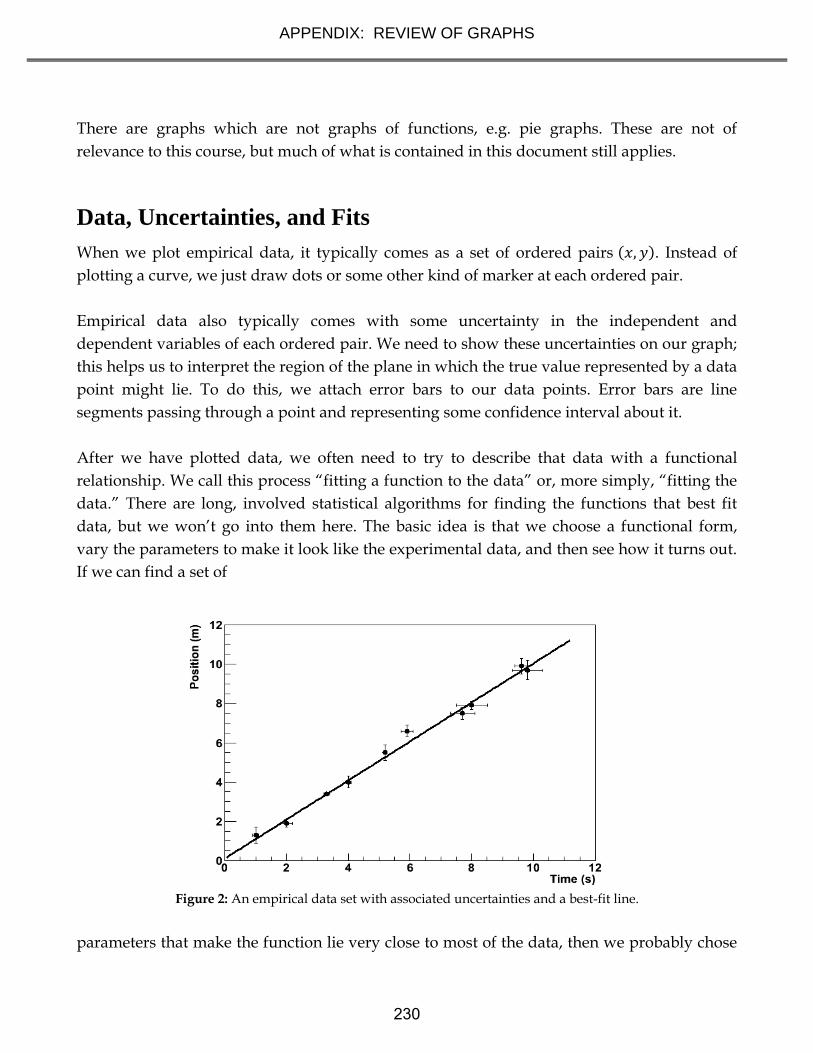
APPENDIX: REVIEW OF GRAPHS
There are graphs which are not graphs of functions, e.g. pie graphs. These are not of
relevance to this course, but much of what is contained in this document still applies.
Data, Uncertainties, and Fits
When we plot empirical data, it typically comes as a set of ordered pairs ( ). Instead of
plotting a curve, we just draw dots or some other kind of marker at each ordered pair.
Empirical data also typically comes with some uncertainty in the independent and
dependent variables of each ordered pair. We need to show these uncertainties on our graph;
this helps us to interpret the region of the plane in which the true value represented by a data
point might lie. To do this, we attach error bars to our data points. Error bars are line
segments passing through a point and representing some confidence interval about it.
After we have plotted data, we often need to try to describe that data with a functional
relationship. We call this process “fitting a function to the data” or, more simply, “fitting the
data.” There are long, involved statistical algorithms for finding the functions that best fit
data, but we won’t go into them here. The basic idea is that we choose a functional form,
vary the parameters to make it look like the experimental data, and then see how it turns out.
If we can find a set of
Figure 2: An empirical data set with associated uncertainties and a best-fit line.
parameters that make the function lie very close to most of the data, then we probably chose
230
APPENDIX: REVIEW OF GRAPHS
the right functional form. If not, then we go back and try again. In this class, we will be
almost exclusively fitting lines because this is easiest kind of fit to perform by eye. Quite
simply, we draw the line through the data points that best models the set of data points in
question. The line is not a “line graph;” we do not just connect the dots (That would almost
never be a line, anyway, but just a series of line segments.). The line does not actually need to
pass through any of the data points. It usually has about half of the points above it and half of
the points below it, but this is not a strict requirement. It should pass through the confidence
intervals around most of the data points, but it does not need to pass through all of them,
particularly if the number of data points is large. Many computer programs capable of
producing graphs have built-in algorithms to find the best possible fits of lines and other
functions to data sets; it is a good idea to learn how to use a high-quality one.
Making Graphs Say Something
So we now know what a graph is and how to plot it; great. Our graph still doesn’t say much;
take the graph in Figure 4(a). What does it mean? Something called apparently varies
quadratically with something called , but that is only a mathematical statement, not a
physical one. We still need to attach physical meaning to the mathematical relationship that
the graph communicates. This is where labels come into play.
Graphs should always have labels on both the horizontal and vertical axes. The labels should
be terse but sufficiently descriptive to be unambiguous. Let’s say that is position and is
time in Figure 4. If the problem is one-dimensional, then the label “Position” is probably
sufficient for the vertical axis ( ). If the problem is two-dimensional, then we probably need
another qualifier. Let’s say that the object in question is moving in a plane and that q is the
vertical component of its position; then “Vertical Position” will probably do the trick. There’s
still a problem with our axis labels. Look more closely; where is the object at ? Who
knows? We don’t know if the ticks represent seconds, minutes, centuries, femtoseconds, or
even some nonlinear measure of time, like humans born. Even if we did, the vertical axis has
no units, either. We need for the units of each axis to be clearly indicated if our graph is really
to say something. We can tell from Figure 4(b) that the object is at at . A grain
of salt: our prediction graphs will not always need units. For example, if we are asked to
draw a graph predicting the relationship of, say, the acceleration due to gravity of an object
with respect to its mass, the label “Mass” will do just fine for our horizontal axis. This is
because we are not expected to give the precise functional dependence in this situation, only
the overall behavior. We don’t know exactly what the acceleration will be at a mass of ,
and we don’t care. We just need to show whether the variation is increasing, decreasing,
constant, linear, quadratic, etc. In this specific case, it might be to our advantage to include
231

APPENDIX: REVIEW OF GRAPHS
units on the vertical axis, though; we can probably predict a specific value of the acceleration,
and that value will be meaningless without them.
(a)
(b) Position q with respect to time τ for a
mass of 3kg. The acceleration is constant.
Figure 4: Poorly- versus well-labeled and -captioned graphs. The labels and caption make the
second graph much easier to interpret.
Every graph we make should also have some sort of title or caption. This helps the reader
quickly to interpret the meaning of the graph without having to wonder what it’s trying to
say. It particularly helps in documents with lots of graphs. Typically, captions are more
useful than just titles. If we have some commentary about a graph, then it is appropriate to
put this in a caption, but not a title. Moreover, the first sentence in every caption should serve
the same role as a title: to tell the reader what information the graph is trying to show. In fact,
if we have an idea for the title of a graph, we can usually just put a period after it and let that
be the first “sentence” in a caption. For this reason, it is typically redundant to include both a
title and a caption. After the opening statement, the caption should add any information
important to the interpretation of a graph that the graph itself does not communicate; this
might be an approximation involved, an indication of the value of some quantity not
depicted in the graph, the functional form of a fit line, a statement about the errors, etc. Lastly,
it is also good explicitly to state any important conclusion that the graph is supposed to
support but does not obviously demonstrate. For example, let’s look at Figure 4 again. If we
are trying to demonstrate that the acceleration is constant, then we would not need to point
this out for a graph of the object’s acceleration with respect to time. Since we did not do that,
but apparently had some reason to plot position with respect to time instead, we wrote, “The
acceleration is constant.”
Lastly, we should choose the ranges of our axes so that our meaning is clear. Our axes do not
232
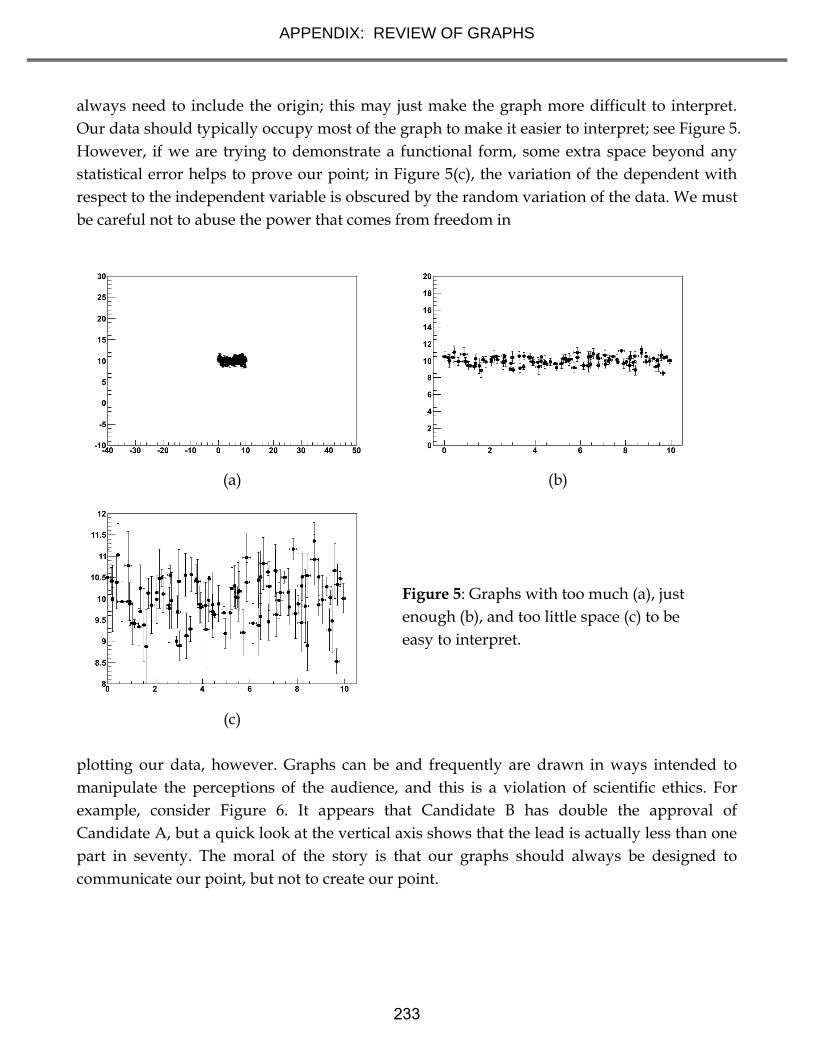
APPENDIX: REVIEW OF GRAPHS
always need to include the origin; this may just make the graph more difficult to interpret.
Our data should typically occupy most of the graph to make it easier to interpret; see Figure 5.
However, if we are trying to demonstrate a functional form, some extra space beyond any
statistical error helps to prove our point; in Figure 5(c), the variation of the dependent with
respect to the independent variable is obscured by the random variation of the data. We must
be careful not to abuse the power that comes from freedom in
(a)
(b)
(c)
Figure 5: Graphs with too much (a), just
enough (b), and too little space (c) to be
easy to interpret.
plotting our data, however. Graphs can be and frequently are drawn in ways intended to
manipulate the perceptions of the audience, and this is a violation of scientific ethics. For
example, consider Figure 6. It appears that Candidate B has double the approval of
Candidate A, but a quick look at the vertical axis shows that the lead is actually less than one
part in seventy. The moral of the story is that our graphs should always be designed to
communicate our point, but not to create our point.
233

APPENDIX: REVIEW OF GRAPHS
Figure 6: Approval
ratings for two
candidates in a mayoral
race. This graph is
designed to mislead the
reader into believing
that Candidate B has a
much higher approval
rating than Candidate
A.
Using Linear Relationships to Make Graphs Clear
The easiest kind of graph to interpret is often a line. Our minds are very good at
interpreting lines. Unfortunately, data often follow nonlinear relationships, and our minds
are not nearly as good at interpreting those. It is sometimes to our advantage to force data to
be linear on our graph. There are two ways that we might want to do this in this class; one is
with calculus, and the other is by cleverly choosing what quantities to graph.
The “calculus” method is the simpler of the two. Don't let its name fool you: it doesn't
actually require any calculus. Let’s say that we want to compare the constant accelerations of
two objects, and we have data about their positions and velocities with respect to time. If the
accelerations are very similar, then it might be difficult to decide the relationship from the
position graphs because we have a hard time detecting fine variations in curvature. It is
much easier to compare the accelerations from the velocity graphs because we then just have
to look at the slopes of lines; see Figure 7. We call this the “calculus” method because velocity
is the first derivative with respect to time of position; we have effectively chosen to plot the
derivative of position rather than position itself. We can sometimes use these calculus-based
relationships to graph more meaningful quantities than the obvious ones.
234
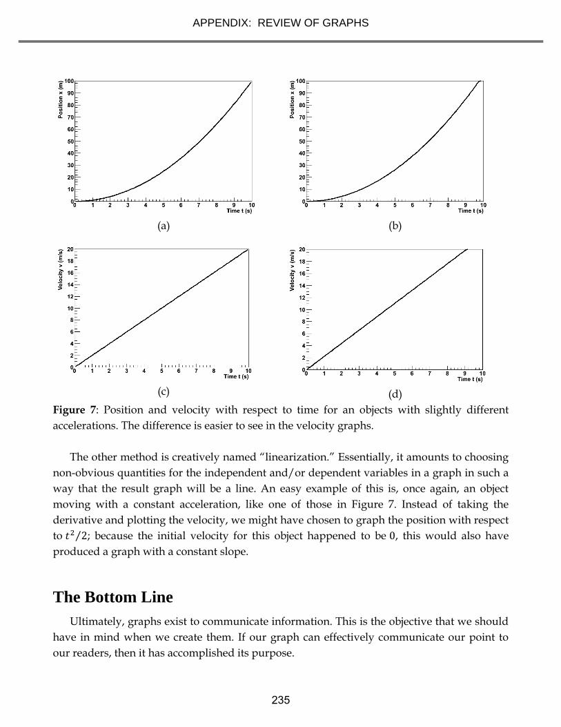
APPENDIX: REVIEW OF GRAPHS
(a)
(b)
(c)
(d)
Figure 7: Position and velocity with respect to time for an objects with slightly different
accelerations. The difference is easier to see in the velocity graphs.
The other method is creatively named “linearization.” Essentially, it amounts to choosing
non-obvious quantities for the independent and/or dependent variables in a graph in such a
way that the result graph will be a line. An easy example of this is, once again, an object
moving with a constant acceleration, like one of those in Figure 7. Instead of taking the
derivative and plotting the velocity, we might have chosen to graph the position with respect
to ⁄ ; because the initial velocity for this object happened to be , this would also have
produced a graph with a constant slope.
The Bottom Line
Ultimately, graphs exist to communicate information. This is the objective that we should
have in mind when we create them. If our graph can effectively communicate our point to
our readers, then it has accomplished its purpose.
235

APPENDIX: REVIEW OF GRAPHS
Figure 8: The position of the first object from Figure 7 plotted with respect to ⁄ . The relationship has been
linearized.
236
Appendix: Guide to Writing Lab Reports (130x)
Many students have a great deal of trouble writing lab reports. They don’t know what a lab report is; they don’t know how to write one; they don’t know what to put in one. This document seeks to resolve those problems. We will address them in that order. This manual includes examples of a good and of a bad lab report; examine them in conjunction with this document to aid your understanding.
What Is a Lab Report?
Everyone seems to understand that a lab report is a written document about an experiment performed in lab. Beyond that, a lab report’s identity is less obvious and more disputed. Let’s save ourselves some misery by first listing some things that a lab report is not. A lab report is not
… a worksheet; you may not simply use the example like a template,substituting what
is relevant for your experiment.
... the story of your experiment; although a description of the experimental procedure
is necessary and very story-like, this is only one part of the much greater analytical
document that is the report.
... rigid; what is appropriate for a report about one experiment may not be appropriate
for another.
... a set of independent sections; a lab report should be logically divided, but its
structure should be natural, and its prose should flow.
So what, then, is a lab report? A lab report is a document beginning with the proposal of a question and then proceeding, using your experiment, to answerthat question. It explains not only what was done, but why it was done and what it means. To try to specify the content in much more detail than this is too constraining; you must simply do whatever is necessary to accomplish these goals. However, a lab report usually accomplishes them in four phases. First, it introduces the experiment by placing it in context, usually the motivation for performing it and some question that it seeks to answer. Second, it describes the methods of the experiment. Third, it analyzes the data to yield some scientifically meaningful result. Fourth, it discusses the result, answering the original question and explaining what the result means. There are, of course, other senses of what a lab report is — it is quantitative, it is persuasive, etcetera — but we will come to those along the way.
237

APPENDIX: GUIDE TO WRITING LAB REPORTS – 130x
How Do I Write a Lab Report?
Now that we have a vague idea of what a lab report is, let’s discuss how to write it. By this, we do not mean its content, but its audience, style, etcetera.
Making an Argument
We already mentioned that a lab report uses an experiment to answer a question, but merely answering it isn’t enough; your report must convince the reader that the answer is correct. This makes a lab report a persuasive document. Your persuasive argument is the single most important part of any lab report. You must be able to communicate and demonstrate a clear point. If you can do this well, your report will be a success; if you cannot, it will be a failure. At some point, you have certainly written a traditional, five-paragraph essay. The first paragraph introduces a thesis, the second through fourth defend the thesis, and the fifth paragraph concludes by restating the thesis. This is a little too simple for a lab report, but the basic idea is the same; keep it in mind. This structure is typically implemented in science in four basic sections: introduction, methodology, results, and discussion. This is sometimes called the “IMRD method.” Begin by stating your thesis, along with enough background information to explain it and a brief preview of how you intend to support it, in your introduction. Defend your thesis in the methodology and results sections. Restate your thesis, this time with a little more critical evaluation, in your discussion. However, keep in mind that IMRD can be a rule or a guideline. In this class, we shall not have exactly four sections with these titles; we shall divide the report more finely (See below.). Roughly speaking, “Introduction” will become the Introduction and Prediction sections, “Methodology” and “Results” will become the Procedure, Data, and Analysis sections, and “Discussion” will become the Conclusion section: introduce and state your prediction in the Introduction and Prediction sections; test your prediction in the Procedure, Data, and Analysis sections; and restate and critically evaluate both your prediction and your result in your Conclusion section.
Audience
If you are successfully to persuade your audience, you must know something about her. What sorts of things does she know about physics, and what sorts of things does she find convincing? For your lab report, she is an arbitrary scientifically-literate person. She is not quite your professor, not quite your TA, and not quite your labmates, but she is this same sort of person. The biggest difference is that she doesn’t know what your experiment is, why you are doing it, or what you hope to prove until you tell her. Use physics and mathematics freely in your report, but explain your experiment and analysis in detail.
Technical Style
A lab report is a technical document. This means that it is stylistically quite different from other documents you may have written. What characterizes technical writing, at least as far
238

APPENDIX: GUIDE TO WRITING LAB REPORTS – 130x
as your lab report is concerned? Here are some of the most prominent features, but for a general idea, read the sample good lab report included in this manual. A lab report does not entertain. When you read the sample reports, you may find them boring; that’s OK. The science in your report should be able to stand for itself. If your report needs to be entertaining, then its science is lacking. A lab report is a persuasive document, but it does not express opinions. Yourprediction should be expressed as an objective hypothesis, and your experiment and analysis should be a disinterested effort to confirm or deny it. Your result may or may not coincide with your prediction, and your report should support that result objectively. A lab report is divided into sections. Each section should clearly communicate one aspect of your experiment or analysis. A lab report may use either the active or the passive voice. Use whichever feels natural and accomplishes your intent, but you should be consistent. A lab report presents much of its information with media other than prose. Tables, graphs, diagrams, and equations frequently can communicate far more effectively than can words. Integrate them smoothly into your report. A lab report is quantitative. If you don’t have numbers to support what you say, you may as well not say it at all. Some of these points are important and sophisticated enough to merit sections of their own, so let’s discuss them some more.
Nonverbal Media
A picture is worth a thousand words. Take this old sentiment to heart when you write your lab report, but do not limit yourself to pictures. Make your point as clearly and tersely as possible; if a graph will do this better than words will, use a graph. When you incorporate these media, you must do so well, in a way that serves the fundamental purpose of clear communication. Label them “Figure 1” and “Table 2.” Give them meaningful captions that inform the reader what information they are presenting. Give them context in the prose of your report. They need to be functional parts of your document’s argument, and they need to be well-integrated into the discussion. Students sometimes think that they are graded “for the graphs,” and TAs sometimes over-emphasize the importance of these media. Avoid these pitfalls by keeping in mind that the purpose of these things is communication. If you can make your point more elegantly with these tools, then use them. If you cannot, then stick to tried-and-true prose. Use your best judgment.
239

APPENDIX: GUIDE TO WRITING LAB REPORTS – 130x
Quantitativeness
A lab report is quantitative. Quantitativeness is the power of scientific analysis. It is objective. It holds a special power lacking in all other forms of human endeavor: it allows us to know precisely how well we know something. Your report is scientifically valid only insofar as it is quantitative. Give numbers for everything, and give the numerical errors in those numbers. If you find yourself using words like “big,” “small,” “close,” “similar,” etcetera, then you are probably not being sufficiently quantitative. Replace vague statements like these with precise, quantitative ones. If there is a single “most important part” to quantitativeness, it is error analysis. This lab manual contains an appendix about error analysis; read it, understand it, and take it to heart.
What Should I Put in My Lab Report?
Structure your report like this.
Abstract
Think of the abstract as your report in miniature. Make it only a few sentences long. State the question you are trying to answer, the method you used to answer it, and your results. It is not an introduction. Your report should make sense in its absence. You do not need to include your prediction here.
Introduction
Do three things in your introduction. First, provide enough context so that your audience can understand the question that your report tries to answer. This typically involves a brief discussion of the hypothetical real-world scenario from the lab manual. Second, clearly state the question. Third, provide a brief statement of how you intend to answer it. It can sometimes help students to think of the introduction as the part justifying your report to your company or funding agency. Leave your reader with an understanding of what your experiment is and why it is important.
Predictions
Include the same predictions in your report that you made prior to the beginning of the experiment. They do not need to be correct. You will do the same amount of work whether they are correct or incorrect, and you will receive far more credit for an incorrect, well-refuted prediction than for a correct, poorly-supported one. Your prediction will often be an equation or a graph. If so, discuss it in prose.
240
APPENDIX: GUIDE TO WRITING LAB REPORTS – 130x
Procedure
Explain what your actual experimental methodology was in the procedure section. Discuss the apparatus and techniques that you used to make your measurements. Exercise a little conservatism and wisdom when deciding what to include in this section. Include all of the information necessary for someone else to repeat the experiment, but only in the important ways. It is important that you measured the time for a cart to roll down a ramp through a length of one meter; it is not important who released the cart, how you chose to coordinate the person releasing it with the person timing it, or which one meter of the ramp you used. Omit any obvious steps. If you performed an experiment using some apparatus, it is obvious that you gathered the apparatus at some point. If you measured the current through a circuit, it is obvious that you hooked up the wires. One aspect of this which is frequently problematic for students is that a step is not necessarily important or non-obvious just because they find it difficult or time-consuming. Decide what is scientifically important, and then include only that in your report. Students approach this section in more incorrect ways than any other. Do not provide a bulleted list of the equipment. Do not present the procedure as a series of numbered steps. Do not use the second person or the imperative mood. Do not treat this section as though it is more important than the rest of the report. You should rarely make this the longest, most involved section.
Data
This should be your easiest section. Record your empirical measurements here: times, voltages, fits from MotionLab, etcetera. Do not use this as the report’s dumping ground for your raw data. Think about which measurements are important to your experiment and which ones are not. Only include data in processed form. Use tables, graphs, and etcetera, with helpful captions. Do not use long lists of measurements without logical grouping or order. Give the units and uncertainties in all of your measurements. This section is a bit of an exception to the “smoothly integrate figures and tables” rule. Include little to no prose here; most of the discussion belongs in the Analysis section. The distinction between the Data and Analysis sections exists mostly for your TA.
Analysis
Do the heavy lifting of your lab report in the Analysis section. Take the data from the Data section, scientifically analyze it, and finally answer the question you posed in your Introduction. Do this quantitatively. Your analysis will almost always amount to quantifying the errors in your measurements and in any theoretical calculations that you made in the Predictions section. Decide whether
241
APPENDIX: GUIDE TO WRITING LAB REPORTS – 130x
the error intervals in your measurements and predictions are compatible. This manual contains an appendix about error analysis; read it for a description of how to do this. If your prediction turns out to be incorrect, then show that as the first part of your analysis. Propose the correct result and show that it is correct as the second part of your analysis. Finally, discuss any shortcomings of your procedure or analysis, such as sources of systematic error for which you did not account, approximations that are not necessarily valid, etcetera. Decide how badly these shortcomings affect your result. If you cannot confirm your prediction, then estimate which are the most important.
Conclusion
Consider your conclusion the wrapping paper and bow tie of your report. At this point, you should already have said most of the important things, but this is where you collect them in one place. Remind your audience what you did, what your result was, and how it compares to your prediction. Tell her what it means. Leave her with a sense of closure. Quote your result from the Analysis section and interpret it in the context of the hypothetical scenario from the Introduction. If you determined that there were any major shortcomings in your experiment, you might also propose future work to overcome them. If the Introduction was your attempt to justify your past funding, then the Conclusion is your attempt to justify your future funding.
What Now?
Read the sample reports included in this manual. There are two; one is an example of these instructions implemented well, and the other is an example of these instructions implemented poorly. Then, talk to your TA. He can answer any remaining questions that you might have. There is a lot of information here, so using it and actually writing your lab report might seem a little overwhelming. A good technique for getting started is this: complete your analysis and answer your question before you ever sit down to write your report. At that point, the hard part of the writing should be done: you already know what the question was, what you did to answer it, and what the answer was. Then just put that do
242
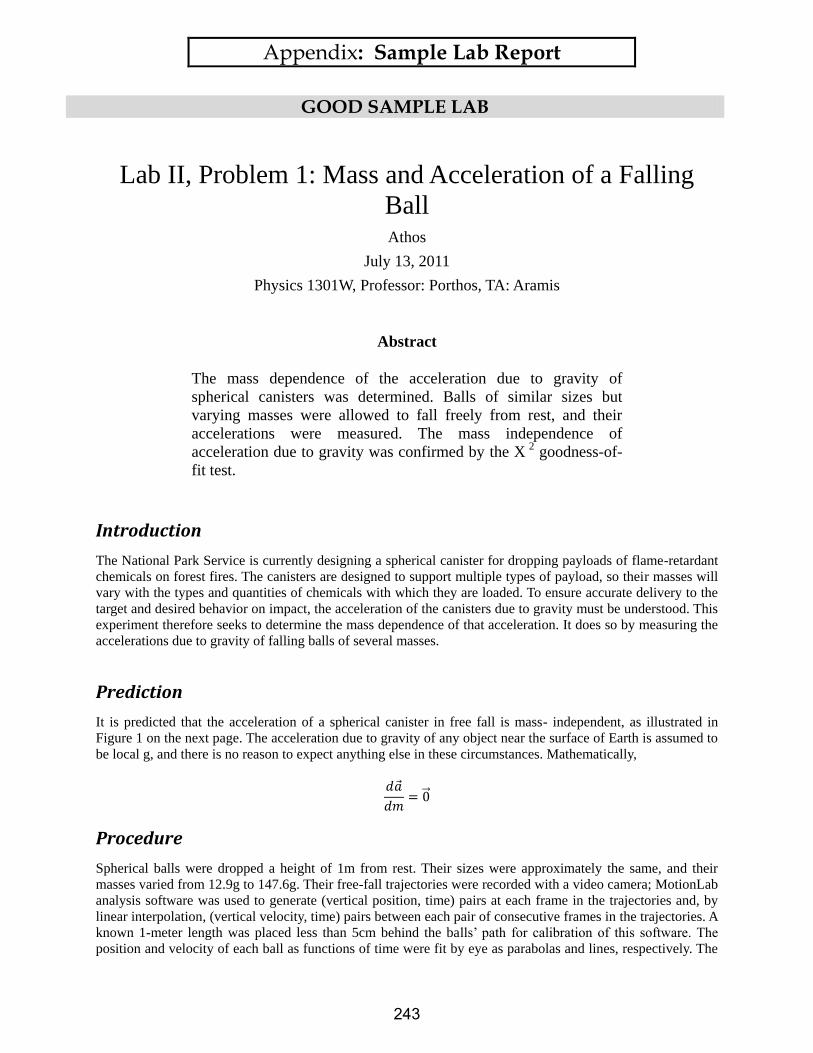
Appendix: Sample Lab Report
GOOD SAMPLE LAB
Lab II, Problem 1: Mass and Acceleration of a Falling
Ball Athos
July 13, 2011
Physics 1301W, Professor: Porthos, TA: Aramis
Abstract
The mass dependence of the acceleration due to gravity of
spherical canisters was determined. Balls of similar sizes but
varying masses were allowed to fall freely from rest, and their
accelerations were measured. The mass independence of
acceleration due to gravity was confirmed by the X 2
goodness-of-
fit test.
Introduction
The National Park Service is currently designing a spherical canister for dropping payloads of flame-retardant
chemicals on forest fires. The canisters are designed to support multiple types of payload, so their masses will
vary with the types and quantities of chemicals with which they are loaded. To ensure accurate delivery to the
target and desired behavior on impact, the acceleration of the canisters due to gravity must be understood. This
experiment therefore seeks to determine the mass dependence of that acceleration. It does so by measuring the
accelerations due to gravity of falling balls of several masses.
Prediction
It is predicted that the acceleration of a spherical canister in free fall is mass- independent, as illustrated in
Figure 1 on the next page. The acceleration due to gravity of any object near the surface of Earth is assumed to
be local g, and there is no reason to expect anything else in these circumstances. Mathematically,
𝑑�⃗�
𝑑𝑚= 0⃗⃗
Procedure
Spherical balls were dropped a height of 1m from rest. Their sizes were approximately the same, and their
masses varied from 12.9g to 147.6g. Their free-fall trajectories were recorded with a video camera; MotionLab
analysis software was used to generate (vertical position, time) pairs at each frame in the trajectories and, by
linear interpolation, (vertical velocity, time) pairs between each pair of consecutive frames in the trajectories. A
known 1-meter length was placed less than 5cm behind the balls’ path for calibration of this software. The
position and velocity of each ball as functions of time were fit by eye as parabolas and lines, respectively. The
243

APPENDIX: SAMPLE LAB REPORT
acceleration of each was then taken to be the slope of the velocity-versus-time graph, as this was deemed to be
more reliably fittable by eye than the quadraticity of the position-versus-time graph.
Data
Figure 1: Magnitude of acceleration due to gravity with respect to mass of a spherical container
near Earth’s surface; the dependence is predicted to be trivial.
𝑀(g) 𝑎(m/s2)
12.9 9.6
48.8 10.2
55.8 9.8
56.7 9.9
57.7 10.0
143.0 9.7
147.6 9.7
Table 1: The masses and magnitudes of acceleration of the 7 balls tested in this experiment. The
uncertainties in all of the masses are 0.3g. The uncertainties in the accelerations are unknown;
see the Analysis section for more information.
Analysis
The accelerations as measured by the velocity fits are given in Table 1 in the Data section. In principle, errors
could have been assigned to the fits by finding the maximal and minimal values of the parameters which yield
apparently valid fits, but not all groups performed such an analysis, and this group did not have access to the
raw data necessary to do so themselves. A method of analysis which does not rely on the errors in the
individual accelerations was therefore attempted. In keeping with the hypothesis, the empirical accelerations
were treated as independent measurements of local 𝑔. A constant was then fit to the data, and the 𝑋2 goodness-
244
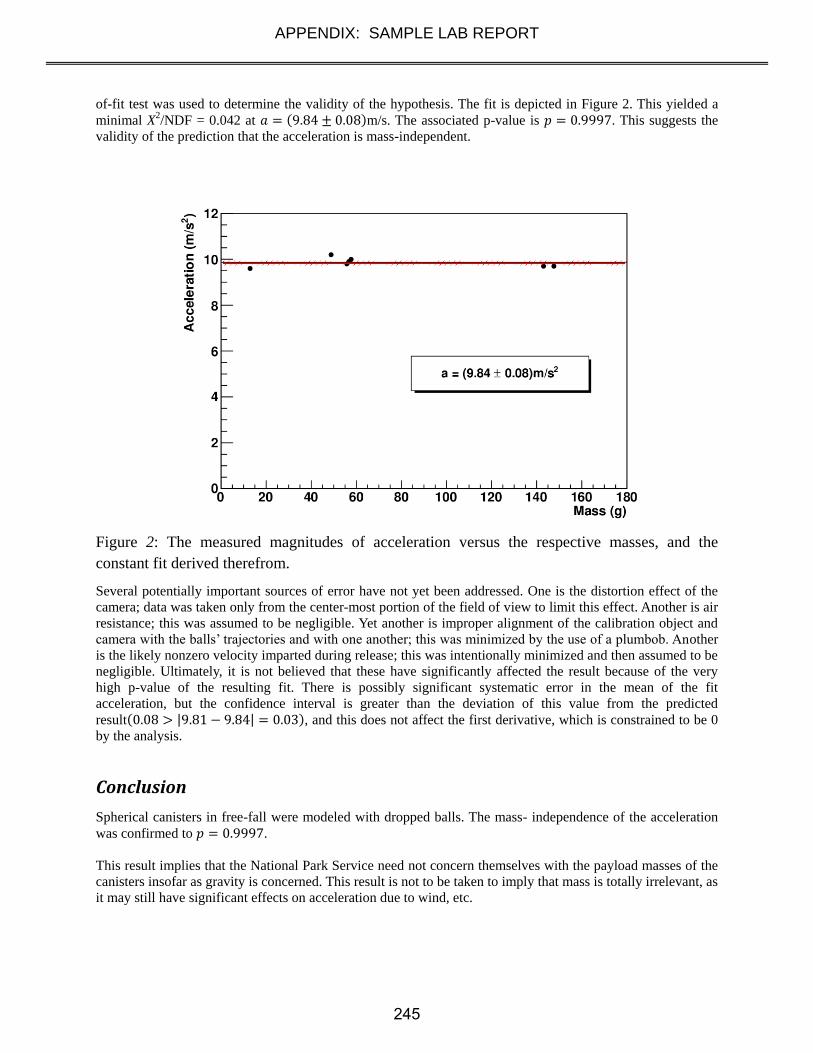
APPENDIX: SAMPLE LAB REPORT
of-fit test was used to determine the validity of the hypothesis. The fit is depicted in Figure 2. This yielded a
minimal X2/NDF = 0.042 at 𝑎 = (9.84 ± 0.08)m/s. The associated p-value is 𝑝 = 0.9997. This suggests the
validity of the prediction that the acceleration is mass-independent.
Figure 2: The measured magnitudes of acceleration versus the respective masses, and the
constant fit derived therefrom.
Several potentially important sources of error have not yet been addressed. One is the distortion effect of the
camera; data was taken only from the center-most portion of the field of view to limit this effect. Another is air
resistance; this was assumed to be negligible. Yet another is improper alignment of the calibration object and
camera with the balls’ trajectories and with one another; this was minimized by the use of a plumbob. Another
is the likely nonzero velocity imparted during release; this was intentionally minimized and then assumed to be
negligible. Ultimately, it is not believed that these have significantly affected the result because of the very
high p-value of the resulting fit. There is possibly significant systematic error in the mean of the fit
acceleration, but the confidence interval is greater than the deviation of this value from the predicted
result(0.08 > |9.81 − 9.84| = 0.03), and this does not affect the first derivative, which is constrained to be 0
by the analysis.
Conclusion
Spherical canisters in free-fall were modeled with dropped balls. The mass- independence of the acceleration
was confirmed to 𝑝 = 0.9997.
This result implies that the National Park Service need not concern themselves with the payload masses of the
canisters insofar as gravity is concerned. This result is not to be taken to imply that mass is totally irrelevant, as
it may still have significant effects on acceleration due to wind, etc.
245
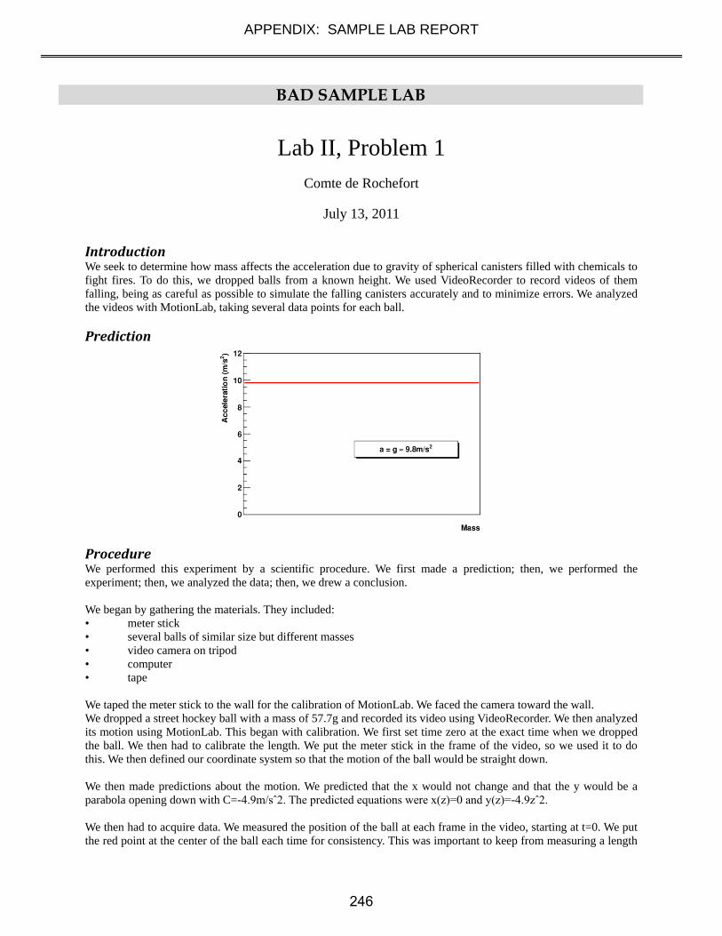
APPENDIX: SAMPLE LAB REPORT
BAD SAMPLE LAB
Lab II, Problem 1
Comte de Rochefort
July 13, 2011
Introduction We seek to determine how mass affects the acceleration due to gravity of spherical canisters filled with chemicals to
fight fires. To do this, we dropped balls from a known height. We used VideoRecorder to record videos of them
falling, being as careful as possible to simulate the falling canisters accurately and to minimize errors. We analyzed
the videos with MotionLab, taking several data points for each ball.
Prediction
Procedure We performed this experiment by a scientific procedure. We first made a prediction; then, we performed the
experiment; then, we analyzed the data; then, we drew a conclusion.
We began by gathering the materials. They included:
• meter stick
• several balls of similar size but different masses
• video camera on tripod
• computer
• tape
We taped the meter stick to the wall for the calibration of MotionLab. We faced the camera toward the wall.
We dropped a street hockey ball with a mass of 57.7g and recorded its video using VideoRecorder. We then analyzed
its motion using MotionLab. This began with calibration. We first set time zero at the exact time when we dropped
the ball. We then had to calibrate the length. We put the meter stick in the frame of the video, so we used it to do
this. We then defined our coordinate system so that the motion of the ball would be straight down.
We then made predictions about the motion. We predicted that the x would not change and that the y would be a
parabola opening down with C=-4.9m/sˆ2. The predicted equations were x(z)=0 and y(z)=-4.9zˆ2.
We then had to acquire data. We measured the position of the ball at each frame in the video, starting at t=0. We put
the red point at the center of the ball each time for consistency. This was important to keep from measuring a length
246

APPENDIX: SAMPLE LAB REPORT
that changed from frame to frame based on where we put the data point on the ball. We also did not use some of the
frames at the end of the video, where the ball was at the edge where the camera is susceptible to the fisheye effect
and where the ball was not in the frame.
When this was finished, we fit functions to the data points. The functions did not fit the points exactly, but they were
acceptably close. We fit x(z)=0 for the x position and y(z)=-5zˆ2 for the y position. These were close to our
predictions.
It then came time to make predictions of the velocity graphs. We predicted that the Vx graph would be a straight line
with Vx(z)=0 and that the Vy graph would be a linear line with Vy(z)=-10z.
Next, we fit the functions to the data points for the velocity graphs. We got the predictions exactly right.
We then printed our data for the street hockey ball and closed MotionLab.
We repeated this process for a baseball with a mass of 143.0g. It was mostly the same, with some exceptions. The
y(z) fit was y(z)=-4.85zˆ2 instead of y(z)=-5zˆ2. The Vy(z) prediction was Vy(z)=-9.7z instead of Vy(z)=-10z. These
were also exactly right, so the Vy(z) fit was the same.
At the end of the lab, everybody put their data on the board so we would have enough to do the analysis. We copied
it down. Then we were finished, so we started the next experiment.
Data Ball 1
mass: 12.9+/-0.05g
x prediction: x=0z
x fit: x=0z
y prediction: y=-4.9zˆ2
y fit: y=-4.8zˆ2
Vx prediction: Vx=0z
Vx fit: Vx=0z
Vy prediction: Vy=-9.6z
Vy fit: Vy=-9.6z
Ball 4
mass: 56.7+/-0.05g
x prediction: x=0z
x fit: x=0z
y prediction: y=-4.9zˆ2
y fit: y=-4.95zˆ2
Vx prediction: Vx=0z
Vx fit: Vx=0z
Vy prediction: Vy=-9.9z
Vy fit: Vy=-9.9z
Ball 2
mass: 48.8+/-0.05g
x prediction: x=0z
x fit: x=0z
y prediction: y=-4.9zˆ2
y fit: y=-5.1zˆ2
Vx prediction: Vx=0z
Vx fit: Vx=0z
Vy prediction: Vy=-10.2z
Vy fit: Vy=-10.2z
Ball 5
mass: 57.7+/-0.05g
x prediction: x=0z
x fit: x=0z
y prediction: y=-4.9zˆ2
y fit: y=-5.0zˆ2
Vx prediction: Vx=0z
Vx fit: Vx=0z
Vy prediction: Vy=-10.0z
Vy fit: Vy=-10.0z
Ball 3
mass: 55.8+/-0.05g
x prediction: x=0z
x fit: x=0z
y prediction: y=-4.9zˆ2
y fit: y=-4.9zˆ2
Vx prediction: Vx=0z
Vx fit: Vx=0z
Vy prediction: Vy=-9.8z
Vy fit: Vy=-9.8z
Ball 6
mass: 143.0+/-0.05g
x prediction: x=0z
x fit: x=0z
y prediction: y=-4.9zˆ2
y fit: y=-4.85zˆ2
Vx prediction: Vx=0z
Vx fit: Vx=0z
Vy prediction: Vy=-9.7z
Vy fit: Vy=-9.7z
247

APPENDIX: SAMPLE LAB REPORT
Ball 7
mass: 147.6+/-0.05g
x prediction: x=0z
x fit: x=0z
y prediction: y=-4.9zˆ2
y fit: y=-4.8zˆ2
Vx prediction: Vx=0z
Vx fit: Vx=0z
Vy prediction: Vy=-9.6z
Vy fit: Vy=-9.7z
Analysis We can calculate the acceleration from the MotionLab fit functions. To do this, we use the formula x =
x0+v0t+1/2atˆ2. Then a is just 2 times the coefficient of zˆ2 in the position fits. This gives us
Ball 1: a=-9.6
Ball 2: a=-10.2
Ball 3: a=-9.8
Ball 4: a=-9.9
Ball 5: a=-10.0
Ball 6: a=-9.7
Ball 7: a=-9.6
The acceleration can also be calculated using the formula v=v0+at. Then
a is just the coefficient of z in the velocity fits. This gives us
Ball 1: a=-9.6
Ball 2: a=-10.2
Ball 3: a=-9.8
Ball 4: a=-9.9
Ball 5: a=-10.0
Ball 6: a=-9.7
Ball 7: a=-9.7
We know that the acceleration due to gravity is -9.8m/sˆ2, so we need to compare the measured values of the
acceleration to this number. Looking at the data from the fits, we can see that they are all close to -9.8m/sˆ2, so the
error in this lab must not be significant. Ball 3 actually had 0 error.
We need to analyze the sources of error in the lab to interpret our result. One is human error, which can never be
totally eliminated. Another error is the error in MotionLab. This is obvious because the data points don’t lie right on
the fit, but are spread out around it. Another error is that the mass balance could only weigh the masses to +/-0.05g,
as shown in the data section. There was error in the fisheye effect of the camera lens. There was air resistance, but
we set that to 0, so it is not important.
Conclusion We predicted that a would be -9.8m/sˆ2, and we measured seven values of a very close to this. None was off by
more than 0.4m/sˆ2, and one was exactly right. The errors are therefore not significant to our result. We can say that
the canisters fall at 9.8m/sˆ2. This experiment was definitely a success.
248