13 Random Variables I - Dept of Math, CCNY
26
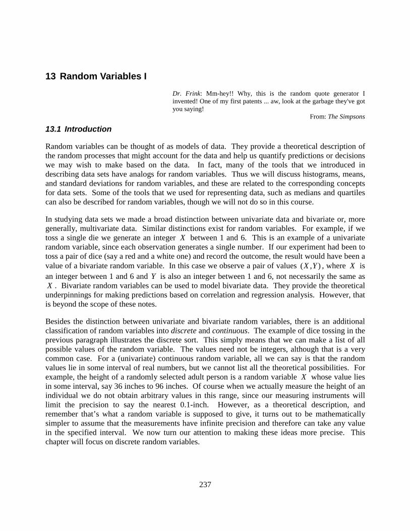
237 13 Random Variables I Dr. Frink: Mm-hey!! Why, this is the random quote generator I invented! One of my first patents ... aw, look at the garbage they've got you saying! From: The Simpsons 13.1 Introduction Random variables can be thought of as models of data. They provide a theoretical description of the random processes that might account for the data and help us quantify predictions or decisions we may wish to make based on the data. In fact, many of the tools that we introduced in describing data sets have analogs for random variables. Thus we will discuss histograms, means, and standard deviations for random variables, and these are related to the corresponding concepts for data sets. Some of the tools that we used for representing data, such as medians and quartiles can also be described for random variables, though we will not do so in this course. In studying data sets we made a broad distinction between univariate data and bivariate or, more generally, multivariate data. Similar distinctions exist for random variables. For example, if we toss a single die we generate an integer X between 1 and 6. This is an example of a univariate random variable, since each observation generates a single number. If our experiment had been to toss a pair of dice (say a red and a white one) and record the outcome, the result would have been a value of a bivariate random variable. In this case we observe a pair of values ( , ) XY , where X is an integer between 1 and 6 and Y is also an integer between 1 and 6, not necessarily the same as X . Bivariate random variables can be used to model bivariate data. They provide the theoretical underpinnings for making predictions based on correlation and regression analysis. However, that is beyond the scope of these notes. Besides the distinction between univariate and bivariate random variables, there is an additional classification of random variables into discrete and continuous. The example of dice tossing in the previous paragraph illustrates the discrete sort. This simply means that we can make a list of all possible values of the random variable. The values need not be integers, although that is a very common case. For a (univariate) continuous random variable, all we can say is that the random values lie in some interval of real numbers, but we cannot list all the theoretical possibilities. For example, the height of a randomly selected adult person is a random variable X whose value lies in some interval, say 36 inches to 96 inches. Of course when we actually measure the height of an individual we do not obtain arbitrary values in this range, since our measuring instruments will limit the precision to say the nearest 0.1-inch. However, as a theoretical description, and remember that’s what a random variable is supposed to give, it turns out to be mathematically simpler to assume that the measurements have infinite precision and therefore can take any value in the specified interval. We now turn our attention to making these ideas more precise. This chapter will focus on discrete random variables.
Transcript of 13 Random Variables I - Dept of Math, CCNY
237
13 Random Variables IDr. Frink: Mm-hey!! Why, this is the random quote generator Iinvented! One of my first patents ... aw, look at the garbage they've gotyou saying!
From: The Simpsons
13.1 Introduction
Random variables can be thought of as models of data. They provide a theoretical description ofthe random processes that might account for the data and help us quantify predictions or decisionswe may wish to make based on the data. In fact, many of the tools that we introduced indescribing data sets have analogs for random variables. Thus we will discuss histograms, means,and standard deviations for random variables, and these are related to the corresponding conceptsfor data sets. Some of the tools that we used for representing data, such as medians and quartilescan also be described for random variables, though we will not do so in this course.
In studying data sets we made a broad distinction between univariate data and bivariate or, moregenerally, multivariate data. Similar distinctions exist for random variables. For example, if wetoss a single die we generate an integer X between 1 and 6. This is an example of a univariaterandom variable, since each observation generates a single number. If our experiment had been totoss a pair of dice (say a red and a white one) and record the outcome, the result would have been avalue of a bivariate random variable. In this case we observe a pair of values ( , )X Y , where X isan integer between 1 and 6 and Y is also an integer between 1 and 6, not necessarily the same asX . Bivariate random variables can be used to model bivariate data. They provide the theoreticalunderpinnings for making predictions based on correlation and regression analysis. However, thatis beyond the scope of these notes.
Besides the distinction between univariate and bivariate random variables, there is an additionalclassification of random variables into discrete and continuous. The example of dice tossing in theprevious paragraph illustrates the discrete sort. This simply means that we can make a list of allpossible values of the random variable. The values need not be integers, although that is a verycommon case. For a (univariate) continuous random variable, all we can say is that the randomvalues lie in some interval of real numbers, but we cannot list all the theoretical possibilities. Forexample, the height of a randomly selected adult person is a random variable X whose value liesin some interval, say 36 inches to 96 inches. Of course when we actually measure the height of anindividual we do not obtain arbitrary values in this range, since our measuring instruments willlimit the precision to say the nearest 0.1-inch. However, as a theoretical description, andremember that’s what a random variable is supposed to give, it turns out to be mathematicallysimpler to assume that the measurements have infinite precision and therefore can take any valuein the specified interval. We now turn our attention to making these ideas more precise. Thischapter will focus on discrete random variables.

13 Random Variables I
238
13.2 Discrete Random Variables
We first give a definition that makes precise the discussion in section 13.1. This will be followedby a number of examples, which should give the reader a more concrete grasp of the concept. Insection 13.3 we will consider some special discrete random variables that have wide applicability.
Definition 13.1: A discrete random variable associated with an experiment is a set of numericaloutcomes 1 2, , , ,nx x x… … such that whenever the experiment is performed one and only one of theoutcomes 1 2, , , ,nx x x… … occurs.!
We will denote random variables using capital letters, for example X or Y . A particular value ofthe random variable will be denoted using a lower case letter, say x or 1x , etc.
Example 13.1: Examples of discrete random variables.
a) If a single die is tossed, the number of dots on the upward facing side defines a randomvariable X whose values are {1, 2,3,4,5,6}. If we toss a pair of dice and record the sum Y ,that is again a random variable whose values are {2,3, 4,5,6,7,8,9,10,11,12}.
b) If we take a survey of 25 people to find whether they support candidate A, then the number ofsupporters of A in the sample surveyed is a random variable X whose values are{0,1, 2, , 24, 25}… . If we are interested in the fraction of people in the survey that supportcandidate A, rather than the number, this is again a discrete random variable Y taking values{0,.04,.08, ,.96,1}… , obtained by dividing the actual number X by 25.
c) If we count the number of cars going through a tollbooth during the same one-minute intervalon various days we have a random variable X whose possible values are {0,1, 2, }… . In thisexample, one could reasonably argue that a value of say 1000 is impossible. However, ratherthan setting an arbitrary cutoff we will deal with this objection by assigning extremely smallprobabilities to such exceptional values.!
So far a random variable only describes what are the possible outcomes of an experiment. To beuseful we must give some information regarding the likelihood of each value.
Definition 13.2: The probability distribution of a discrete random variable is the set ofprobabilities 1 2, , ,np p p… … associated with the outcomes 1 2, , , ,nx x x… … .!
For a discrete random variable, it is often convenient to exhibit the values and their associatedprobabilities in a table, which is often referred to as the probability distribution.
Example 13.2: Find the probability distributions for the random variables in Example 13.1.
Solution:

13 Random Variables I
239
The probability distributions for the random variables X and Y in Example 13.1a) are easilyobtained from our work with probabilities in Chapters 10 and 11. Namely, for tossing a single diewe have:
X 1 2 3 4 5 6( )P X x= 1/6 1/6 1/6 1/6 1/6 1/6
The first row of the probability distribution lists the values of the random variable. The secondrow lists the associated probabilities. The lead entry in the second row, ( )P X x= , can be read as“the probability that the random variable X takes on the value x ”. In this example theprobabilities associated with the six values of the random variable are all 1/6, since any side hasequal chance of facing upwards.
For the sum of two dice Y we have the following probability distribution.
Y 2 3 4 5 6 7( )P Y y= 1/36 2/36 3/36 4/36 5/36 6/36
Y 8 9 10 11 12( )P Y y= 5/36 4/36 3/36 2/36 1/36
Table 13.1
The entry under 4Y = for instance asserts that ( 4)P Y = is 3/36. This result is obtained from ourbasic probability analysis of this experiment, as described in Example 10.6 of Chapter 10. Thereare three toss combinations (1,3), (2, 2), (3,1) out of 36 possible outcomes that produce a sum of thedice equal to 4.
What are the probability distributions for parts b) and c) of Example 13.1? This cannot beanswered without further knowledge of the underlying processes. As we will see in section 13.3the distribution for b) depends on the percent of voters favoring candidate A, while in c) theprobabilities depend on the average number of vehicles crossing during the particular one-minutetime period.!
In each of the tables given above, the sum of the probabilities totals one. This is because ourdefinition of random variable required that whenever the experiment is performed one and onlyone value of the random variable must be obtained. Thus the events 1E = { X has value 1x } ,
2E = { X has value 2x } ,… nE = { X has value nx ,… } are mutually exclusive and exactly oneof them is certain to occur. Thus
1 2 n 1 2 n 1 21= (E or E or or E or ) (E ) (E ) (E ) nP P P P p p p= + + + + = + + + +… … " " " " .
We summarize this as a rule.
13 Random Variables I
240
Rule 13.1 (Unity Rule): If X is a discrete random variable with values 1 2, , ,nx x x… … andassociated probabilities 1 2, , ,np p p… … , with 0ip ≥ then 1 2 1np p p+ + + + =" " .!
Rather than give the probability distribution in tabular form it is visually more appealing to presentit graphically. The resulting graph is called the probability histogram of the discrete randomvariable.
Definition 13.3: The probability histogram of the random variable X whose probabilitydistribution is given by the table
X 1x 2x … nx …
( )P X x= 1p 2p … np …
is a column chart whose horizontal axis shows the values 1 2, , nx x x… arranged in increasing order,with a thin bar centered around each value ix and having height equal to the correspondingprobability ip .!
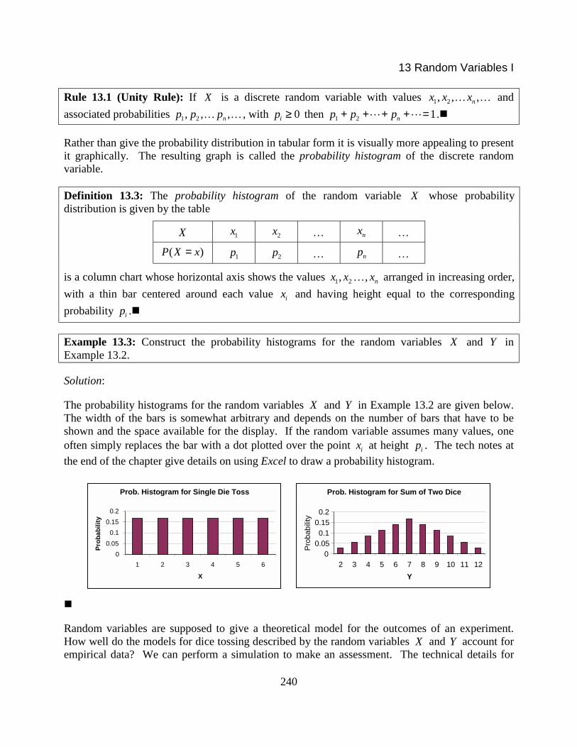
Example 13.3: Construct the probability histograms for the random variables X and Y inExample 13.2.
Solution:
The probability histograms for the random variables X and Y in Example 13.2 are given below.The width of the bars is somewhat arbitrary and depends on the number of bars that have to beshown and the space available for the display. If the random variable assumes many values, oneoften simply replaces the bar with a dot plotted over the point ix at height ip . The tech notes atthe end of the chapter give details on using Excel to draw a probability histogram.
Prob. Histogram for Single Die Toss
00.05
0.10.15
0.2
1 2 3 4 5 6
X
Prob
abili
ty
Prob. Histogram for Sum of Two Dice
00.050.1
0.150.2
2 3 4 5 6 7 8 9 10 11 12Y
Prob
abilit
y
!
Random variables are supposed to give a theoretical model for the outcomes of an experiment.How well do the models for dice tossing described by the random variables X and Y account forempirical data? We can perform a simulation to make an assessment. The technical details for

13 Random Variables I
241
how to do this in Excel are described in the tech notes. Chapter 14 goes a little more deeply intothe theory behind these simulations.
Example 13.4: Simulate the tossing a single die 500 times. Compare the results with thetheoretical probability distribution.
Solution:
The table below shows the results of a simulation of 500 tosses of a single die. The relativefrequencies in row 3 are obtained from the actual frequencies in row 2 by dividing each entry inthe latter row by 500.
Outcome, x 1 2 3 4 5 6Simulation Freq. 80 80 77 76 94 93
Simulation Rel. Freq. .16 .16 .154 .152 .188 .186( )P X x= .166 .166 .166 .166 .166 .166
Table 13.2
There is generally good agreement between the empirical relative frequencies in row 3 and thetheoretical probabilities in row 4. A statistical procedure known as the chi-square test may be usedto show that the deviations exhibited are well within the expected variations for this type ofexperiment. The empirical relative frequencies and the theoretical probabilities may also becompared graphically as in the figure below. The bars are used to represent the theoreticalprobability histogram and the connected points show the relative frequency for the data.
Single Die Toss: Theory & Data
0
0.1
0.2
0.3
0.4
1 2 3 4 5 6X
Rel
. Fre
q. o
r Pro
b.
TheoryData
13 Random Variables I
Similar graphs can be obtained using the simulation program dice.xls, except that the empiricalfrequencies are plotted with bars and the theoretical values, after the user enters them, are plottedas a connected line.!
As was mentioned in the introduction, we can define numerical measures associated with a randomvariable that capture the flavor of the mean and standard deviation for data. Consider theexperiment that is summarized in Table 13.2. What is the average of the 500 tosses? To obtainthis we must add the values found in all 500 tosses and then divide by 500. The sum of the tossescan be obtained using the information in rows 1 and 2. Namely,
sum = (1 80) + (2 80) + (3 77) + (4 76) + (5 94) + (6 93)=1803× × × × × × (13.1)
Note the similarity with the method used in section 7.6 on estimating the mean and standarddeviation. In this case though the data is naturally grouped into the values 1, 2, 3, etc. and theabove calculation is not an approximation but the exact value of the sum of the tosses. To obtainthe mean of the tosses we divide the sum by 500, the number of tosses, obtaining 3.606. For ourimmediate purposes it is more important to examine the form of the answer, rather than itsnumerical value. In computing the value of sum/ 500 we can divide each term on the right side of(13.1) by the denominator 500, obtaining
sum 80 80 77 76 94 93mean = 1 2 3 4 5 6500 500 500 500 500 500 500
= × + × + × + × + × + ×
(1 0.16) (2 0.16) (3 0.154) (4 0.152) (5 0.188) (6 0.186)= × + × + × + × + × + × .
In the latter form for the mean, each value 1 to 6 is weighted with the relative frequency withwhich it occurred in the experiment. Since these relative frequencies are approximations to thetheoretical probabilities (compare rows 3 and 4 in Table 13.2) we are lead to the followingdefinition for the theoretical mean of a discrete random variable.
Definition 13.4: The expected value or mean of a random variable X having a discrete probabilitydistribution given by the table
X 1x 2x … nx …
( )P X x= 1p 2p … np …
is the quantity denoted by ( )E X or Xµ and defined as
1 1 2 2( ) X n nE X x p x p x pµ= = + + + +" " .!
Remark: µ is the Greek letter mu, which of course should bring to mind the analogous mean of adata set. Do not make the mistake of dividing the sum given in Definition 13.4 by the number ofvalues of the random variable. For a random variable, the averaging is accomplished with theweighting factors ip , each of which accounts for the frequency with which a value ix is supposed
!!!!
242
to occur.

13 Random Variables I
243
Example 13.5: Find the expected value for the toss of a single die and for the sum of the tossestwo dice.
Solution:
The expected value of the random variable X given by the toss of a single die is
1 1 1 1 1 1 1 211 2 3 4 5 6 (1 2 3 4 5 6) 3.56 6 6 6 6 6 6 6
× + × + × + × + × + × = × + + + + + = = .
Note that this answer is close to the average 3.6 observed in the simulation of Example 13.4. Asthe number of tosses increases the average for an actual sample is very likely to get close to thetheoretical average given by ( )E X . This important point will be explored further in Chapter 15.
For the random variable Y that gives the sum of two tosses, a calculation using the probabilitydistribution in Table 13.1 yields that ( ) 7E Y = . Note that this is twice the average or expectedvalue for the toss of a single die. This is not surprising, since Y is just the sum of the valuesobtained on each individual die.!
Example 13.6: A box contains 50 balls, of which 10 are black and 40 are red. Consider playingthe following game. For the price of $1 you are blindfolded and allowed to reach into the box todraw a ball. If the ball is black you receive back $4; if it is red you get back nothing and thus losethe $1 you paid to play. If you play this game repeatedly, on average how much will you win orlose?
Solution:
The question involves a calculation of a theoretical average. We can do this by constructing arandom variable that describes the possible outcomes of playing the game. Let us call this randomvariable X . We need to list the values of the random variable and then the probabilitiesassociated with each. There are two values for X . If you draw a black ball you will have made$3 (the difference between what you get back and the fee to play). If you draw a red ball you willsimply lose $1. We can represent this as a value of -1 for X . Since the probability of selecting ared ball is 40/50 = 4/5 and the probability of selecting a black ball is 10/50 = 1/5 we have thefollowing probability distribution for X .
X -1 3( )P X x= 4/5 1/5
Thus 4 1 1( 1) 35 5 5Xµ = − × + × = − , so that, on average, you will lose 1/5 of a dollar, or 20¢ each
play. In the tech notes we will see how this experiment may be simulated and the theoreticalaverage approximated by the data average.!

13 Random Variables I
244
In summarizing data we needed, in addition to the average, a measure of how the data values arespread around the average. We want a similar measure for random variables.
Definition 13.5: The standard deviation of a random variable X from its mean µ is the numberdenoted by Xσ or just σ and defined by
2 2 21 1 2 2( ) ( ) ( )n nx p x p x pσ µ µ µ= − + − + + − +" " .
The variance, varX , of a random variable X is the square of the standard deviation, i.e.2varX Xσ= .!
The symbol σ is the Greek letter sigma, meant to suggest the Latin letter s used to represent thestandard deviation of a set of data. The definition of σ has the same spirit as the definition of µ .Both are weighted averages. In σ , we square the deviation of each value ix from the mean valueµ . We weight each squared deviation with the frequency or probability ip with which thecorresponding value ix occurs. The outer square root has the same purpose as it does for thestandard deviation of data, namely, to express the answer in similar units as the quantities ix .
Example 13.7: Compute the standard deviation for the random variables X and Y in Example13.2.
Solution:
We have for X ,
2 2 2 2 2 21 1 1 1 1 1(1 3.5) (2 3.5) (3 3.5) (4 3.5) (5 3.5) (6 3.5) 1.716 6 6 6 6 6Xσ = − + − + − + − + − + − ≈
The terms under the radical give the variance. Its exact value is var 17.5 6 2.92X = ≈ . For thesimulated dice tossing experiment given in Table 13.2, the standard deviation of the data set is1.74, which compares favorably with the theoretical value of Xσ computed above.
For the sum of two dice, using a similar computation with Table 13.1, we find that 2.42Yσ ≈ and2 2var (2.42) 5.86Y Yσ= ≈ ≈ . Note that though the standard deviation of the random variable Y is
greater than that of X , it is not twice as great, as was the relationship between the expectedvalues. Remarkably though, the variance of Y is precisely double the variance of X , althoughbecause of round off this is not exactly realized in the above computations. From the relationship
2 22Y Xσ σ= we obtain that 2Y Xσ σ= . We will return to this issue in Chapter 15.!
We will get a better idea of the significance of the standard deviation in the next section as well asin our discussion of the normal distribution in Chapter 14.

13 Random Variables I
245
13.3 The Binomial Distribution
Example 13.8: Four unrelated people walk into a blood donation center. Suppose X is thenumber of these who are of type A. Find the probability distribution of X .
Solution:
Clearly the possible values of X are 0, 1, 2, 3, 4. The difficulty is in computing the probability ofeach of these outcomes. The extreme possibilities are easy. 0X = means that none of the donorswas of type A. Based on the data in Chapter 11, Example 11.1, we know that ( ) .4P A = andtherefore that ( ) .6cP A = . Since the donors are unrelated, the events that none of them are of typeA are independent and so the probability that 0X = is given by 4(.6) .13≈ . Similarly,
4( 4) (.4) .026P X = = ≈ .
To find ( 1)P X = we must examine the possible ways this event can occur. To simplify thenotation let us use S (for success) when a donor has type A, and F (for failure) otherwise. Therandom variable X will have value 1 when exactly one out of the four donors has type A. Thereare four possible ways in which this can happen: SFFF or FSFF or FFSF or FFFS. Usingindependence, the probability of the sequence SFFF is 3(.40)(.60) .086≈ . The other threearrangements also have the same probability and since they are mutually exclusive we can add theprobabilities to get the probability of SFFF or FSFF or FFSF or FFFS. Thus
3( 1) 4(.40)(.60) .346P X = = ≈ .
To obtain ( 2)P X = we list all possible ways in which exactly two out of the four donors could beof type A. We obtain the following list: SSFF or SFSF or SFFS or FSSF or FSFS or FFSS. Anyone of these six outcomes has the same chance of occurring, which independence gives as
2 2(.40) (.60) . Thus 2 2( 2) 6(.40) (.60) .346P X = = ≈ .
Finally, the reader should check that 3( 3) 4(.40) (.60) .154P X = = ≈ . The results are summarizedin tabular form below.
X 0 1 2 3 4( )P X x= .130 .346 .346 .154 .026
The sum of the probabilities in the second row is 1.002 instead of the theoretically correct value of1 as stated in the Unity Rule. This is caused by round-off errors in the decimal values listed in thetable.!
Example 13.8 illustrates a random variable of the binomial type. Such a variable arises in thefollowing situation. We perform an experiment in which we focus on one particular outcome thatwe consider a success, and which we label S. Any other outcome of the experiment is considereda failure, denoted by F. The experiment is performed n times in such a way that the outcomes on

13 Random Variables I
246
each trial are independent of each other. The quantity X giving the number of successes obtainedin the n trials is called a binomial random variable. The following rule gives the formula for theprobability distribution of such a random variable.
Rule 13.2 (Binomial Distribution): Suppose a certain outcome S (success) of an experiment has aprobability p of occurring whenever the experiment is carried out. The complement of S,denoted by F, will then occur with probability 1q p= − . Let X denote the number of successesobtained when the experiment is repeated independently n times. X is a discrete randomvariable. Its probability distribution is given by
X 0 1 2 " k " n( )P X k= nq 1
1n
n C pq − 2 22
nn C p q − " k n k
n kC p q − " np
The numbers n kC appearing as coefficients in row 2 are called binomial coefficients and are givenby the formula
!!( )!n k
nCk n k
=−
.!
• We have deviated slightly from our usual convention of denoting generic values of a randomvariable X with the letter x . Here we denote an unspecified value of X by the letter k toemphasize that we are dealing with integer values.
• Since we are performing the experiment n times the number of successes must certainly beone of the numbers 0, 1, 2, … n , as listed in the table.
• The event that 0X = means we had no successes in the n trials so that all n outcomes werefailures. Thus, using independence of the trials we have ( 0) (F and F and F)= nP X P q= = …as stated in the second row. The probability for all successes, ( ) nP X n p= = , can be obtainedby similar reasoning. These two special cases should be available at your fingertips, so it isgood to understand them independently of the general result.
• The symbol !k is read “ k factorial.” We remind the reader that for 1k ≥ we have! ( 1) 2 1k k k= × − × × ×" . In order that the general formula remain valid for 0k = and k n=
we conventionally define 0! 1= . The binomial coefficients n kC count the number of ways inwhich k successes can appear in the sequence of n trials. For example,
4 24! 4 3 2 1 4 3 6
2!2! (2 1) (2 1) 2 1C × × × ×= = = =
× × × ×,
which the reader can check in Example 13.8 was the number of ways that two suitable donorscould appear in the group of four. In computing binomial coefficients by hand one should first

13 Random Variables I
247
perform the numerous cancellations of common factors in the numerator and denominator.Thus
40 6
40(39)(38)(37)(36)(35) (34!)40!
34! 6!C = =
34!
( 40
6!=
5
) ( 3913
)(38)(37) ( 366
) ( 357
)
6 ( 5 )( 4 )( 3 )( 23,838, 380
)=
• The independence of the trials implies that a particular sequence of n trials that produces ksuccesses has a probability of occurring given by (1 )k n k k n kp p p q− −− = . The previousparagraph tells us that there are n kC such outcomes and this implies the general probabilityformula stated in the table. Notice the structure of the formula. The probability p of successis raised to the power k , which is the number of successes we are interested in. The exponentof q , the failure probability, is then the number of failures n k− in the sequence of n trials.
Example 13.9: Compute the probabilities in Example 13.8 using the formula for the binomialdistribution.
Solution:
Using the binomial distribution requires one to identify two “parameters”, namely the probabilityp of success and the number n of trials. (It is also important to make sure that the trials are
independent.) Here .4p = and therefore 1 .6q p= − = and 4n = . To three decimal places, theprobabilities are given by:
4( 0) .6 .130P X = = =
1 3 3 3 34 1
4! 4 3 2 1( 1) (.4) (.6) (.4)(.6) (.4)(.6) 4(.4)(.6) .3461!3! 3 2 1
P X C × × ×= = = = = =× ×
2 2 2 2 2 2 2 24 2
4! 4 3 2 1( 2) (.4) (.6) (.4) (.6) (.4) (.6) 6(.4) (.6) .3462!2! (2 1)(2 1)
P X C × × ×= = = = = =× ×
3 1 3 1 3 34 3
4! 4 3 2 1( 3) (.4) (.6) (.4) (.6) (.4) (.6) 4(.4) (.6) .1543!1! 3 2 1
P X C × × ×= = = = = =× ×
4( 4) (.4) .026P X = = = !
The computation of binomial coefficients is quite formidable, although many calculators now havethis capability built-in. In the tech notes section we indicate how this may be done in Excel.Appendix B gives three place tables of the binomial distribution for various probabilities ofsuccess and 2,3, 15n = … . These can be used as a convenient substitute for the formula or astatistical program.
Example 13.10: A coin is tossed 10 times. Using the tables find the probability that the number ofheads obtained will be 4, 5 or 6.

13 Random Variables I
248
Solution:
The value of .5p = and we are performing 10n = trials. In appendix section B.1 find the entryfor 10n = and then look at the column headed with .50 at the top. The probability of gettingexactly 4 heads is listed in the column headed with a k . The entry for 4k = (successes) is .205,for 5 successes is .246 and for 6 successes is .205. The probability of getting 4 or 5 or 6 heads isthe sum of the three probabilities, which is .656.!
When the number of trials is large we are often more interested in knowing the probability that thenumber of successes falls in a certain range, rather than the individual probabilities. In this case itis more useful to have a table of cumulative probabilities. Symbolically, this is the probability
( ) ( 0) ( 1) ( 2) ( )P X k P X P X P X P X k≤ = = + = + = + + =" .
The tables in section B.2 give these cumulative probabilities for 20, 25n = and 30. Let's see howthey are used.
Example 13.11: A certain standardized exam has a pass rate of .70, i.e. 70 % of students who takethe exam pass it. If the exam is administered to 25 randomly selected students determine thefollowing probabilities.
a) The probability that 15 or fewer students will pass.
b) The probability that 20 or more will pass.
c) The probability that the number of students who pass, X , will satisfy 15 20X≤ ≤ .
a) We need ( 15)P X ≤ . The table entry for 15k = gives this value as .189. Therefore, it is verylikely that the number of passing students will exceed 15.
b) The table gives the probabilities up to a certain point, whereas this question asks for theprobability beyond a certain point. However, we can use complementation to express the latterprobability in terms of cumulative ones. Namely,
( 20) 1 ( 20) 1 ( 19) 1 .807 .193P X P X P X≥ = − < = − ≤ = − = .
Notice that the complement of getting 20 or more passes is getting strictly fewer than 20.Since the number of successes can only be an integer this is equivalent to 19X ≤ .
c) We want (15 20) ( 15) ( 16) ( 20)P X P X P X P X≤ ≤ = = + = + + =" . We can obtain this fromthe cumulative probability through 20 by removing the contribution of all terms where X issmaller than 15. In other words, we have
(15 20) ( 20) ( 15) ( 20) ( 14) .910 .098 .812P X P X P X P X P X≤ ≤ = ≤ − < = ≤ − ≤ = − = !
One might ask why we don't include any tables for the binomial distribution beyond 30n = . Ofcourse one obvious answer is that such tables would take up too much space. This is quite true,
13 Random Variables I
249
but a more important reason is that such tables are not necessary. As we will see in the nextchapter, when n is larger than 30 (and as long as p is neither too close to zero or one) thebinomial distribution can be approximated quite easily using the normal or bell-shaped distributionthat we have referred to earlier in the course.
At this point it is instructive to take a look at the histogram of the binomial distribution. The filedistributions.xls allows one to easily examine these histograms as well as the numerical values ofthe binomial distribution probabilities and cumulative probabilities.
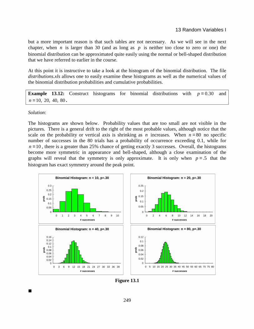
Example 13.12: Construct histograms for binomial distributions with 0.30p = and10, 20, 40, 80n = .
Solution:
The histograms are shown below. Probability values that are too small are not visible in thepictures. There is a general drift to the right of the most probable values, although notice that thescale on the probability or vertical axis is shrinking as n increases. When 80n = no specificnumber of successes in the 80 trials has a probability of occurrence exceeding 0.1, while for
10n = , there is a greater than 25% chance of getting exactly 3 successes. Overall, the histogramsbecome more symmetric in appearance and bell-shaped, although a close examination of thegraphs will reveal that the symmetry is only approximate. It is only when .5p = that thehistogram has exact symmetry around the peak point.
Binomial Histogram: n = 10, p=.30
0
0.050.1
0.15
0.20.25
0.3
0 1 2 3 4 5 6 7 8 9 10 # successes
prob
Binomial Histogram: n = 20, p=.30
0
0.05
0.1
0.15
0.2
0.25
0 2 4 6 8 10 12 14 16 18 20 # successes
prob
Binomial Histogram: n = 40, p=.30
00.020.040.060.08
0.10.120.140.16
0 3 6 9 12 15 18 21 24 27 30 33 36 39 # successes
prob
Binomial Histogram: n = 80, p=.30
0
0.02
0.04
0.06
0.08
0.1
0.12
0 5 10 15 20 25 30 35 40 45 50 55 60 65 70 75 80
# successes
prob
Figure 13.1
!
13 Random Variables I
250
In our later work we will need to know the mean and standard deviation of the binomialdistribution. These can be derived from the general formulas for the distribution, but we will sparethe reader the details.
Rule 13.3: If X has a binomial distribution with n trials and probability of success p then
X npµ = , X npqσ = and the variance is varX npq= .!
The formula for the mean µ is quite plausible. For example, if 40n = and .3p = as in Example13.12, we would have 40 .3 12µ = × = , so that on average we would have 12 successes. Noticethat the histogram in Figure 13.1 for 40n = reaches its peak at approximately 12n = and similarlyfor the other histograms the peak occurs at approximately np . Thus np is also the most probablenumber of successes, though as remarked above the probability of hitting this value exactlybecomes quite small when the number of trials n is large.
The formula for the standard deviation is not intuitively obvious. However, it quantifies an aspectof the histograms that is very important to appreciate and which we will use extensively instatistical inference. In the histograms in Figure 13.1 the values plotted along the horizontal axisdouble as we double n . This is not surprising, since this axis represents the number of possiblesuccesses and we are doubling that from 10n = to 20 up to 80n = . Of course as n increasesmost of the probabilities for the number of successes are too small to show on the graph, whichbecomes concentrated on a steadily smaller fraction of the horizontal axis. As we will show later,this phenomenon is driven by the formula for the standard deviation and in particular that as nincreases, σ only grows like the n rather than like n .
Example 13.13: Compute the mean and standard deviation for the binomial distributions exhibitedin Figure 13.1.
Solution:
In each case we have .3p = and therefore .7q = . The formulas in Rule 13.3 then give thefollowing values for the mean and standard deviation.
n 10 20 40 80µ 10 .3 3× = 20 .3 6× = 40 .3 12× = 80 .3 24× =
σ 10 .3 .7 1.45× × ≈ 20 .3 .7 2.05× × ≈ 40 .3 .7 2.90× × ≈ 80 .3 .7 4.10× × ≈
The means double as we double n , but the standard deviation only increases by a factor of 2with each doubling of n . Thus although the spread (as measured by σ ) is increasing it does somuch more slowly than does the entire range of values for X . As a result the histogram becomesmore concentrated in appearance as n increases.!

13 Random Variables I
251
13.4 The Poisson Distribution
The Poisson (pronounced Pwah-sone) Distribution is named after the mathematician Siméon-Denis Poisson who discovered it in the 1830s. Mathematically this distribution approximates thebinomial distribution when the value of p is small and the value of n is large. For example,
0.02p = and 150n = . This approximation was useful in the pre-computer world, since theprobabilities for the Poisson distribution are easier to calculate than the formulas for the binomialdistribution. As a practical matter this particular use of the Poisson distribution is now of littleimportance. However, for reasons we will see in the next chapter, the distribution arises in othercontexts that make it a very useful model for certain types of data. For example, the situationdescribed in Example 13.1c) involving cars passing through a tollbooth can often be modeledusing a Poisson distribution.
Unlike the other discrete random variables we have considered in this chapter, the Poissondistribution can take on infinitely many values, 0, 1, 2, … . The probability distribution dependson one parameter, usually denoted by the Greek letter λ , (lambda). The meaning of thisparameter will be discussed later, but for now note that λ can be any positive real number and isnot restricted to being an integer.
Definition 13.6 (Poisson Distribution): A random variable X has a Poisson distribution withparameter λ if X can take on any of the values 0, 1, 2, … with probabilities given by thefollowing distribution table:
X 0 1 2 " k "
( )P X k= e λ− e λλ −2
2!e λλ −
"!
kek
λλ −
"
!
Example 13.14: Construct a probability table for a Poisson distribution with 1.5λ = . Display theprobabilities to three decimal places.
Solution:
Using 1.5λ = in Definition 13.6 we have
X 0 1 2 3 4 5 6 7( )P X k= 0.223 0.335 0.251 0.126 0.047 0.014 0.004 0.001
The 8 probabilities shown in the table sum to one, at least to the displayed accuracy. Of coursethis is not exactly correct as in fact the remaining probabilities are non-zero but very small. Forexample,

13 Random Variables I
252
8 1.51.5( 8) .000148!eP X
−
= = ≈ . !
The parameter λ that appears in the definition of the Poisson distribution has a very simpleinterpretation, as stated in the next theorem. We omit the proof of this result, which involves someproperties of the exponential function that are beyond the prerequisites for the course.
Rule 13.4: If X has a Poisson distribution with parameter λ then we have Xµ λ= , Xσ λ= andvarX λ= .!
Thus the quantity λ is the average or mean value of the random variable. This fact is important inmost applications of the Poisson distribution, in particular the application to the binomialdistribution referred to earlier. The idea is to compare a binomial distribution having parametersp and n with a Poisson distribution with parameter npλ = . In doing this we insure that the two
distributions have the same mean, which would certainly be a requirement if they were toapproximate each other. Using the file distributions.xls we can compare the two distributions andjudge the adequacy of the approximation.
Example 13.15: Compare the binomial distributions having parameters
a) 0.02p = and 150n =
b) 0.2p = and 150n =
with suitable Poisson distributions.
a) According to the preceding discussion we should use a Poisson distribution with150 0.02 3npλ = = × = . Figure 13.2 below shows the histogram of the binomial distribution
and a superimposed line graph that plots the Poisson probabilities ( 3λ = ) for the same valuesof each random variable. There is a very close agreement between the two, and the numericaltable given below the histogram confirms this.
Probability Histograms
00.05
0.10.15
0.20.25
0 1 2 3 4 5 6 7 8 9# of Successes
Prob
abili
ty
BinomialPoisson
Figure 13.2
13 Random Variables I
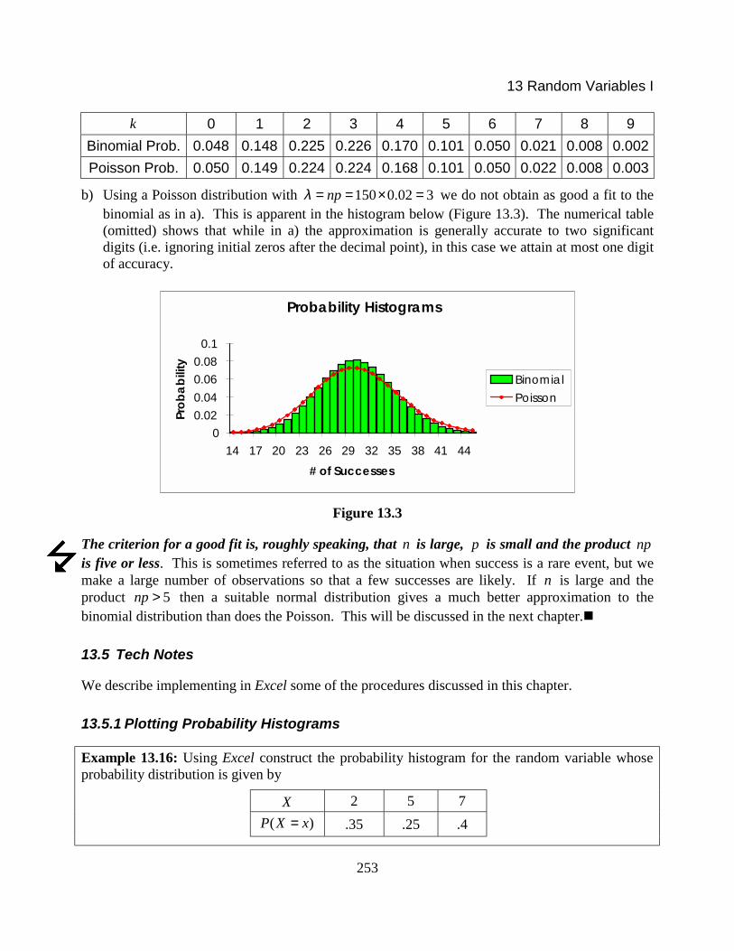
k 0 1 2 3 4 5 6 7 8 9Binomial Prob. 0.048 0.148 0.225 0.226 0.170 0.101 0.050 0.021 0.008 0.002Poisson Prob. 0.050 0.149 0.224 0.224 0.168 0.101 0.050 0.022 0.008 0.003
b) Using a Poisson distribution with 150 0.02 3npλ = = × = we do not obtain as good a fit to thebinomial as in a). This is apparent in the histogram below (Figure 13.3). The numerical table(omitted) shows that while in a) the approximation is generally accurate to two significantdigits (i.e. ignoring initial zeros after the decimal point), in this case we attain at most one digitof accuracy.
Probability Histograms
00.020.040.060.08
0.1
14 17 20 23 26 29 32 35 38 41 44# of Successes
Prob
abili
ty
BinomialPoisson
Figure 13.3
The criterion for a good fit is, roughly speaking, that n is large, p is small and the product npis five or less. This is sometimes referred to as the situation when success is a rare event, but wemake a large number of observations so that a few successes are likely. If n is large and the
!!!!
253
product 5np > then a suitable normal distribution gives a much better approximation to thebinomial distribution than does the Poisson. This will be discussed in the next chapter.!
13.5 Tech Notes
We describe implementing in Excel some of the procedures discussed in this chapter.
13.5.1 Plotting Probability Histograms
Example 13.16: Using Excel construct the probability histogram for the random variable whoseprobability distribution is given by
X 2 5 7( )P X x= .35 .25 .4

13 Random Variables I
254
Solution:
To plot the histogram correctly the X values in the plot must be uniformly spaced. If this is notthe case we can often arrange for it by adding extra X values to which we assign zero probability.In a blank spreadsheet enter the table as a vertical array including all integer values between 2 and7 and assigning probability zero to the extraneous values. See the figure below. Include the texttitles so you know what the numbers refer to.
X 2 3 4 5 6 7( )P X x= 0.35 0 0 0.25 0 0.4
Open the chart wizard.
Step 1: Accept the default column chart type and go to step 2.
Step 2: Enter the reference or select the cells in the probability column of your table. Youshould see a bar chart, but the horizontal axis will not yet be correctly labeled. Clickson the Series tab and in the box labeled “Category (X) axis labels” enter the referenceor select the cells containing the X values.
Step 3: Add a title, label the horizontal axis as X or some more descriptive term. The Y axislabel should be “Probability”. Delete the legend; it is not needed when there is onlyone set of bars.
Step 4: Send the graph to the current worksheet. The final result should look as shown below.You can then modify it to suit your tastes.
Probability Histogram
0
0.1
0.2
0.3
0.4
0.5
2 3 4 5 6 7X
Prob
abili
ty
!
13.5.2 Generating Random Numbers
Example 13.17: Use Excel to simulate generating values for the random variable described inExample 13.6.
13 Random Variables I
255
Solution:
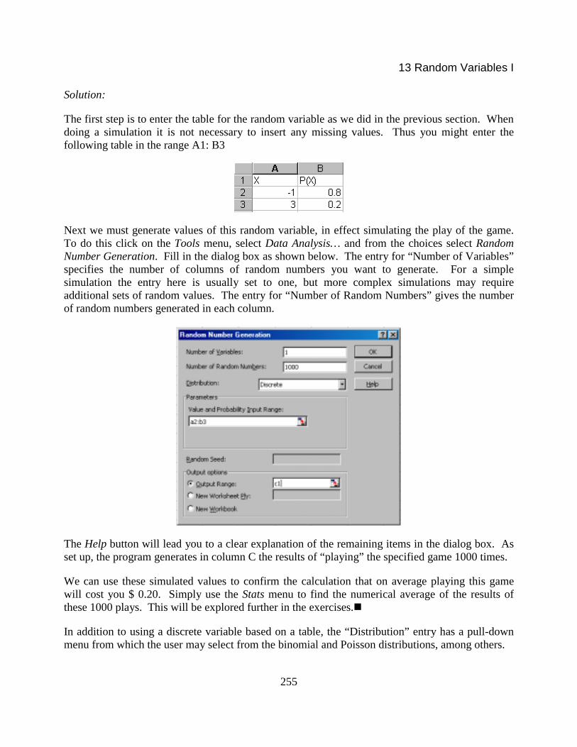
The first step is to enter the table for the random variable as we did in the previous section. Whendoing a simulation it is not necessary to insert any missing values. Thus you might enter thefollowing table in the range A1: B3
Next we must generate values of this random variable, in effect simulating the play of the game.To do this click on the Tools menu, select Data Analysis… and from the choices select RandomNumber Generation. Fill in the dialog box as shown below. The entry for “Number of Variables”specifies the number of columns of random numbers you want to generate. For a simplesimulation the entry here is usually set to one, but more complex simulations may requireadditional sets of random values. The entry for “Number of Random Numbers” gives the numberof random numbers generated in each column.
The Help button will lead you to a clear explanation of the remaining items in the dialog box. Asset up, the program generates in column C the results of “playing” the specified game 1000 times.
We can use these simulated values to confirm the calculation that on average playing this gamewill cost you $ 0.20. Simply use the Stats menu to find the numerical average of the results ofthese 1000 plays. This will be explored further in the exercises.!
In addition to using a discrete variable based on a table, the “Distribution” entry has a pull-downmenu from which the user may select from the binomial and Poisson distributions, among others.

13 Random Variables I
256
13.5.3 Computation of Binomial & Other Probabilities
Many probability distributions can be computed using built-in Excel functions. As it is difficult toremember the exact specifications needed to compute each function, you will want to use thefunction “wizard” to assist you.
Example 13.18: Use the function wizard to compute probabilities for the binomial distribution.
Solution:
Clicking on the toolbar button labeled xf activates the wizard. Scroll down to the list of Statisticalfunctions (or use the category, Most Recently Used, if that is relevant). To obtain probabilityvalues for a binomial distribution, select BINOMDIST. A dialog box opens. Most of the valuesthat you need to enter (except for the last one) should be quite clear to you based on our discussionof the binomial distribution and the explanations in the box. For example, to compute ( 3)P X = ifX has a binomial distribution with .25p = and 8n = fill out the entries as shown below:
The entry “False” for the cumulative field indicates that we wish only the specific probability of 3successes. If we wanted the probability ( 3)P X ≤ we would enter the value “true” in this field.When you have completed entering the values click OK. The formula=BINOMDIST(3,8,.25,FALSE) will be entered in the active cell and the value .207… will appearin the spreadsheet. There is a similar function for computing values of the Poisson distribution.!
13.6 Summary
Flips of a coin, tosses of a die, arrivals and departures from a queue, may appear as simply randomphenomena. However, underlying the randomness are patterns that can be described byprobability theory. The notion of a random variable provides the theoretical mathematicalframework for this description. A random variable has two essential features: first, a clearstatement of the possible values of this random quantity, and second, a probability distributionthat associates with each outcome a certain probability for its occurrence. In this chapter, we haveconsidered discrete random variables, in which the numerical outcomes can be listed. Random
13 Random Variables I
257
phenomena in which the possible outcomes can assume an entire interval of values will beconsidered in Chapter 14.
Since a random variable provides a theoretical model for random data, there are analogues formany of the constructions used in descriptive statistics. Thus, we can represent a discrete randomvariable graphically using a probability histogram. The central tendency and spread of thedistribution can be summarized through the mean (expected value), µ , and the standarddeviation, σ .
There are a number of theoretical discrete random variables that appear as models of many randomexperiments. We have described the binomial and Poisson distributions. The binomialdistribution occurs when we count the number of times an outcome of interest to us (success)occurs in repeated independent trials of an experiment. The Poisson distribution approximates thebinomial distribution when the probability of success is small, but a rather large number of trialstake place. As we will elaborate in the next chapter, this random variable also appears as thenatural distribution in time or space for phenomena that occur infrequently.
13.7 Exercises
1. Determine which of the following describe discrete or continuous random variables, or notrandom variables at all. Justify your answer. It is not necessary to give the probabilitydistribution.
a) The number of days in May.
b) The number of days in a randomly selected month. (Consider only non-leap years.)
c) The length of time it takes you to commute to school each day.
d) The number of misspelled words on page 237 (first page of this chapter) of these notes.
e) Your grade on the final exam in this course.
2. a) Find the missing value in the following probability distribution:
X 1 2 4 6( )P X x= 0.2 0.3 .15 ?
b) For the random variable in a) what is ( 1 or 4)P X X= = ?
c) A random variable X takes on the values 1, 2, or 3x = with probabilities given by theformula ( ) ( 1)P X x xα= = + . Find the value of α and write the probability distributiontable for X .
3. a) What is the probability distribution for the random variable in 1b)?
b) Draw a probability histogram for the distribution you found in 3a).
13 Random Variables I
258
4. For 52 weeks a housewife kept careful records of the number of times she went to thesupermarket each week. The table below summarizes the data she collected. For example, thebolded cells indicate that on seven weeks out of the 52 weeks she made only one trip to thesupermarket.
y = number of trips per week 0 1 2 3 4
# of weeks with y trips 1 7 16 19 9
a) Using the information provided by the table construct a probability distribution table forthe random variable Y = # of trips made each week.
b) Find Yµ . In simple terms explain the meaning of this number.
5. Suppose that X has the following probability distribution table:
X -2 0 2 3 5( )P X x= 0.1 0.2 0.2 0.4 0.1
a) Draw a probability histogram for X .
b) What is (0 3)P X≤ ≤ ?
c) Find Xµ , Xσ and varX .
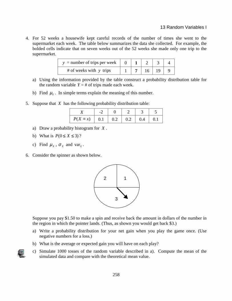
6. Consider the spinner as shown below.
1 2
3
Suppose you pay $1.50 to make a spin and receive back the amount in dollars of the number inthe region in which the pointer lands. (Thus, as shown you would get back $3.)
a) Write a probability distribution for your net gain when you play the game once. (Usenegative numbers for a loss.)
b) What is the average or expected gain you will have on each play?
c) Simulate 1000 tosses of the random variable described in a). Compute the mean of thesimulated data and compare with the theoretical mean value.

13 Random Variables I
259
d) Submit to your instructor the mean of the data for your simulation in c). Construct a boxplot of all the means obtained by students in the class. What is the IQR for the collectionof means?
7. a) Verify the assertion made in the text that the standard deviation for the sum of two dice isapproximately 2.42. (Note: You can use the symmetry of the probability distribution Table13.1 to simplify the calculations.)
b) Use the program dice.xls to generate the sum of 10,000 tosses of two dice. Enter thetheoretical probabilities and print out the sheet showing the frequency tally and thecombined histograms.
c) From the frequency table for the 10,000 tosses that you obtained in b) use the estimationmethod discussed in Chapter 7 section 7.6 to approximate the mean and standard deviationof the data and compare with theoretical values for the random variable.
8. Use Binomial Distribution (Rule 13.2) to verify the values in the tables in Appendix B for thefollowing binomial random variables.
a) ( 3)P X = , where X has 7n = and .2p = .
b) ( 6)P X = , where X has 10n = and .7p = .
9. a) If X has a binomial distribution with 12n = and 0.30p = find (2 6)P X≤ ≤ .
b) If X has a binomial distribution with 25n = and 0.30p = find (6 9)P X≤ ≤ .
10. a) If Y has a binomial distribution with 25n = and 0.75p = , find to three decimal places( 20)P Y = .
b) A certain professor is known to give As to only 10% of her classes. In a class of 30students
i) What is the expected number of As?
ii) Using a suitable table, determine the probability that there will be three or fewer As in aclass of 30.
11. A bowl contains 3 black balls and 7 red ones. You select a ball from the bowl 12 times, withreplacement. Let X equal the number of times a red ball is drawn.
a) Using the formula for the binomial distribution, find the probability that exactly four of theballs selected are red. Check your answer using the tables.
b) Using a table, find the probability that the number of red balls selected will be between 3and 6, inclusive.
12. A multiple-choice test has 10 questions, each with 5 choices for the answer.
13 Random Variables I
260
a) If you guess the answer to each question, use an appropriate table to find the probabilitythat you will get four or more correct answers.
b) What is the expected or average number of questions you will correctly guess? Describethe statistical meaning of this answer.
13. a) A random variable X has a Poisson distribution with 4.5λ = . Compute each of thefollowing probabilities.
i) ( 2)P X = ii) ( 2)P X > iii) (2 5)P X≤ ≤
b) A random variable X has a binomial distribution with 150n = and .03p = . Thefollowing table gives some probabilities for this random variable.
X 2 3 4 5 6( )P X k= 0.1108 0.1691 0.1922 0.1736 0.1297( )P Y k=
Use a suitable random variable Y with a Poisson distribution to estimate the probabilitiesin row 2 and enter these estimates in row 3 of the table. Verify that the results provideestimates for the answers in row 2 that are correct to two significant figures.
14. Suppose that a rare illness strikes about 35 out of 10,000 children per year.
a) What is the probability that a randomly selected child will contract this illness during asingle year?
b) Letting X denote the number of cases of illness among 1000 children, use a binomialdistribution to fill in the missing entries in the table below.
X 0 1 2 3 4 5( )P X k=
c) What is the expected number of cases of the illness amongst a group of 1000 children?
d) Use a random variable Y with a suitable Poisson distribution to estimate the missingprobabilities in b).
e) In a community with 1000 children, how likely would it be that in each of two consecutiveyears more than three cases of the illness would be reported? What assumptions are youusing in your calculations?
15. Consider binomial distributions each having .4p = with 10, 20, 40, 80, and 160n = .
a) Find Xµ and Xσ for each of these.
13 Random Variables I
261
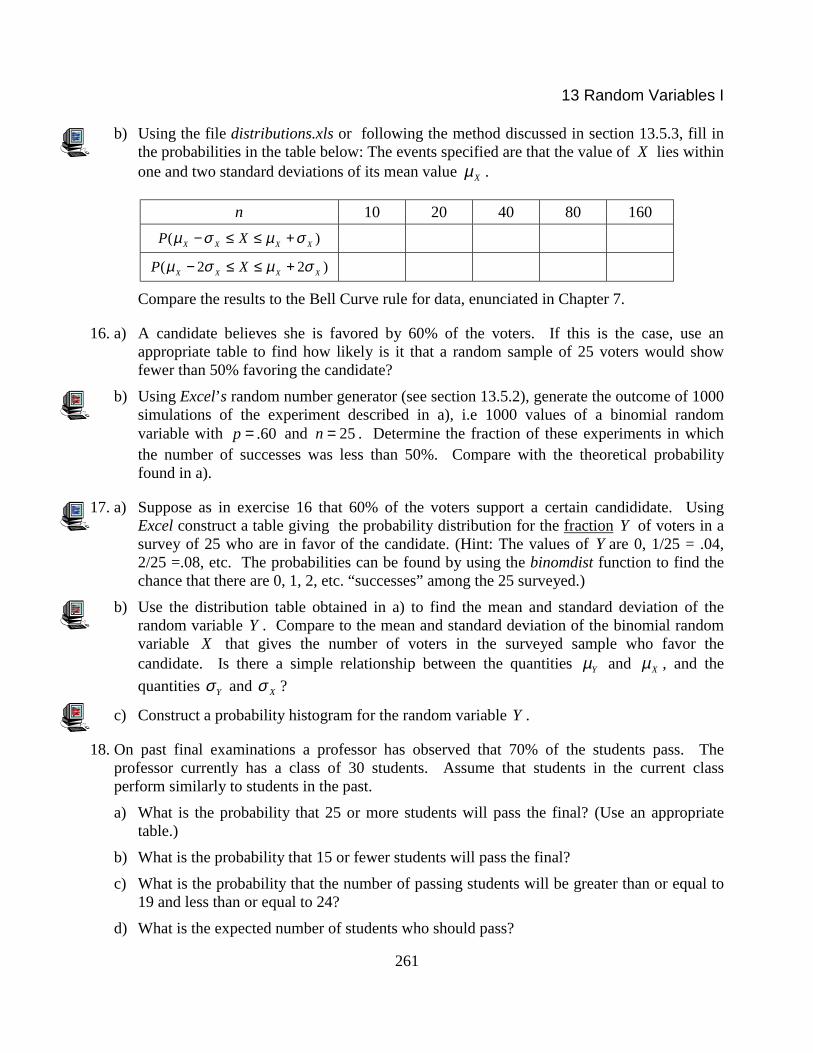
b) Using the file distributions.xls or following the method discussed in section 13.5.3, fill inthe probabilities in the table below: The events specified are that the value of X lies withinone and two standard deviations of its mean value Xµ .
n 10 20 40 80 160( )X X X XP Xµ σ µ σ− ≤ ≤ +
( 2 2 )X X X XP Xµ σ µ σ− ≤ ≤ +
Compare the results to the Bell Curve rule for data, enunciated in Chapter 7.
16. a) A candidate believes she is favored by 60% of the voters. If this is the case, use anappropriate table to find how likely is it that a random sample of 25 voters would showfewer than 50% favoring the candidate?
b) Using Excel’s random number generator (see section 13.5.2), generate the outcome of 1000simulations of the experiment described in a), i.e 1000 values of a binomial randomvariable with .60p = and 25n = . Determine the fraction of these experiments in whichthe number of successes was less than 50%. Compare with the theoretical probabilityfound in a).
17. a) Suppose as in exercise 16 that 60% of the voters support a certain candididate. UsingExcel construct a table giving the probability distribution for the fraction Y of voters in asurvey of 25 who are in favor of the candidate. (Hint: The values of Y are 0, 1/25 = .04,2/25 =.08, etc. The probabilities can be found by using the binomdist function to find thechance that there are 0, 1, 2, etc. “successes” among the 25 surveyed.)
b) Use the distribution table obtained in a) to find the mean and standard deviation of therandom variable Y . Compare to the mean and standard deviation of the binomial randomvariable X that gives the number of voters in the surveyed sample who favor thecandidate. Is there a simple relationship between the quantities Yµ and Xµ , and thequantities Yσ and Xσ ?
c) Construct a probability histogram for the random variable Y .
18. On past final examinations a professor has observed that 70% of the students pass. Theprofessor currently has a class of 30 students. Assume that students in the current classperform similarly to students in the past.
a) What is the probability that 25 or more students will pass the final? (Use an appropriatetable.)
b) What is the probability that 15 or fewer students will pass the final?
c) What is the probability that the number of passing students will be greater than or equal to19 and less than or equal to 24?
d) What is the expected number of students who should pass?

13 Random Variables I
262
19. a) A computer manufacturer claims that at most 1% of the products shipped are defective. Astore receives shipments of 20 computers. Assuming the worst case scenario, what fractionof shipments to the store will have at least one defective computer?
b) Using Excel’s random number generation, simulate making 1000 shipments of 20computers from the manufacturer described in a), assuming that there are 1% defectives ineach shipment. What fraction of the 1000 shipments contain at least one defectivecomputer? How does this number compare with the probability you computed in a)?
20. The median M of a random variable X is defined as a value of X such that bothprobabilities ( )P X M≤ and ( )P X M≥ are greater than 0.5. Using the cumulative binomialdistribution tables, find the median for the following binomial distributions:
a) 20n = , .6p = , .2p =
b) 25n = , .6p = , .2p =
c) Do your answers in a) and b) show any relationship to the expected value of thecorresponding random variables? Based on the analogy of data and probabilitydistributions, why might you expect this relationship to be valid?