1.3 Credit spread and bond price-based pricing

Market’s assessment of the default risk of the obligor (assuming

some form of market efficiency – information is aggregated in the

market prices). The sources are

• market prices of bonds and other defaultable securities issued

by the obligor• prices of CDS’s referencing this obligor’s credit risk

How to construct a clean term structure of credit spreads from

observed market prices?

? Based on no-arbitrage pricing principle, a model that is based

upon and calibrated to the prices of traded assets is immune to

simple arbitrage strategies using these traded assets.

Market instruments used in bond price-based pricing

• At time t, the defaultable and default-free zero-coupon bond

prices of all maturities T ≥ t are known. These defaultable

zero-coupon bonds have no recovery at default.

• Information about the probability of default over all time hori-

zons as assessed by market participants are fully reflected when

market prices of default-free and defaultable bonds of all matu-

rities are available.

Risk neutral probabilities

The financial market is modeled by a filtered probability space (Ω,

(Ft)t≥0,F , Q), where Q is the risk neutral probability measure.

• All probabilities and expectations are taken under Q. Probabili-

ties are considered as state prices.

1. For constant interest rates, the discounted Q-probability of

an event A at time T is the price of a security that pays off

$1 at time T if A occurs.

2. Under stochastic interest rates, the price of the contingent

claim associated with A is E[β(T )1A], where β(T ) is the dis-

count factor. This is based on the risk neutral valuation prin-

ciple and the money market account M(T ) =1

β(T )= e

∫ Tt ru du

is used as the numeraire.

Indicator functions

For A ∈ F ,1A(ω) =

1 if ω ∈ A0 otherwise

.

τ = random time of default; I(t) = survival indicator function

I(t) = 1τ>t =

1 if τ > t0 if τ ≤ t

.

B(t, T ) = price at time t of zero-coupon bond paying off $1 at T

B(t, T ) = price of defaultable zero-coupon bond if τ > t;

I(t)B(t, T ) =

B(t, T ) if τ > t0 if τ ≤ t

.

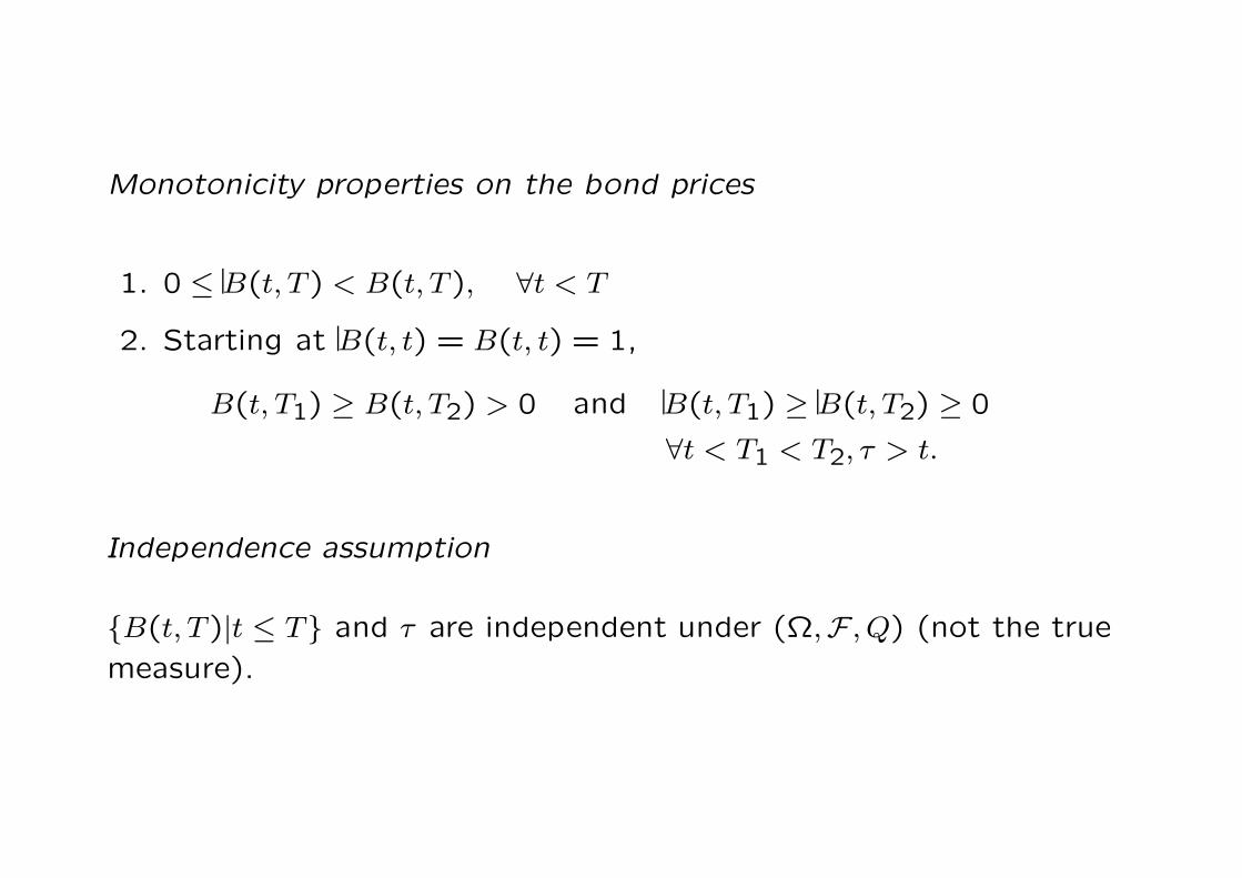
Monotonicity properties on the bond prices

1. 0 ≤ B(t, T ) < B(t, T ), ∀t < T

2. Starting at B(t, t) = B(t, t) = 1,

B(t, T1) ≥ B(t, T2) > 0 and B(t, T1) ≥ B(t, T2) ≥ 0

∀t < T1 < T2, τ > t.

Independence assumption

B(t, T )|t ≤ T and τ are independent under (Ω,F , Q) (not the true

measure).

Implied probability of survival in [t, T ]– based on market prices

of bonds

B(t, T ) = E[e−∫ Tt ru du

]and B(t, T ) = E

[e−∫ Tt ru duI(T )

].

Invoking the independence between defaults and the default-free

interest rates

B(t, T ) = E

[e−∫ Tt ru du

]E[I(T )] = B(t, T )P(t, T )

implied survival probability over [t, T ] = P(t, T ) =B(t, T )

B(t, T ).

• The implied default probability over [t, T ], Pdef(t, T ) = 1−P(t, T ).• Assuming P(t, T ) has a right-sided derivative in T , the implied

density of the default time

Q[τ ∈ (T, T + dT ]|Ft] = −∂

∂TP(t, T ) dT.

• If prices of zero-coupon bonds for all maturities are available,

then we can obtain the implied survival probabilities for all ma-

turities (complementary distribution function of the time of de-

fault).

Properties on implied survival probabilities, P(t, T )

1. P(t, t) = 1 and it is non-negative and decreasing in T . Also,

P(t,∞) = 0.2. Normally P(t, T ) is continuous in its second argument, except

that an important event secheduled at some time T1 has direct

influence on the survival of the obligor.3. Viewed as a function of its first argument t, all survival proba-

bilities for fixed maturity dates will tend to increase.

If we want to focus on the default risk over a given time interval in

the future, we should consider conditional survival probabilities.

conditional survival probability over [T1, T2] as seen from t

= P(t, T1, T2) =P(t, T2)

P(t, T1), where t ≤ T1 < T2.

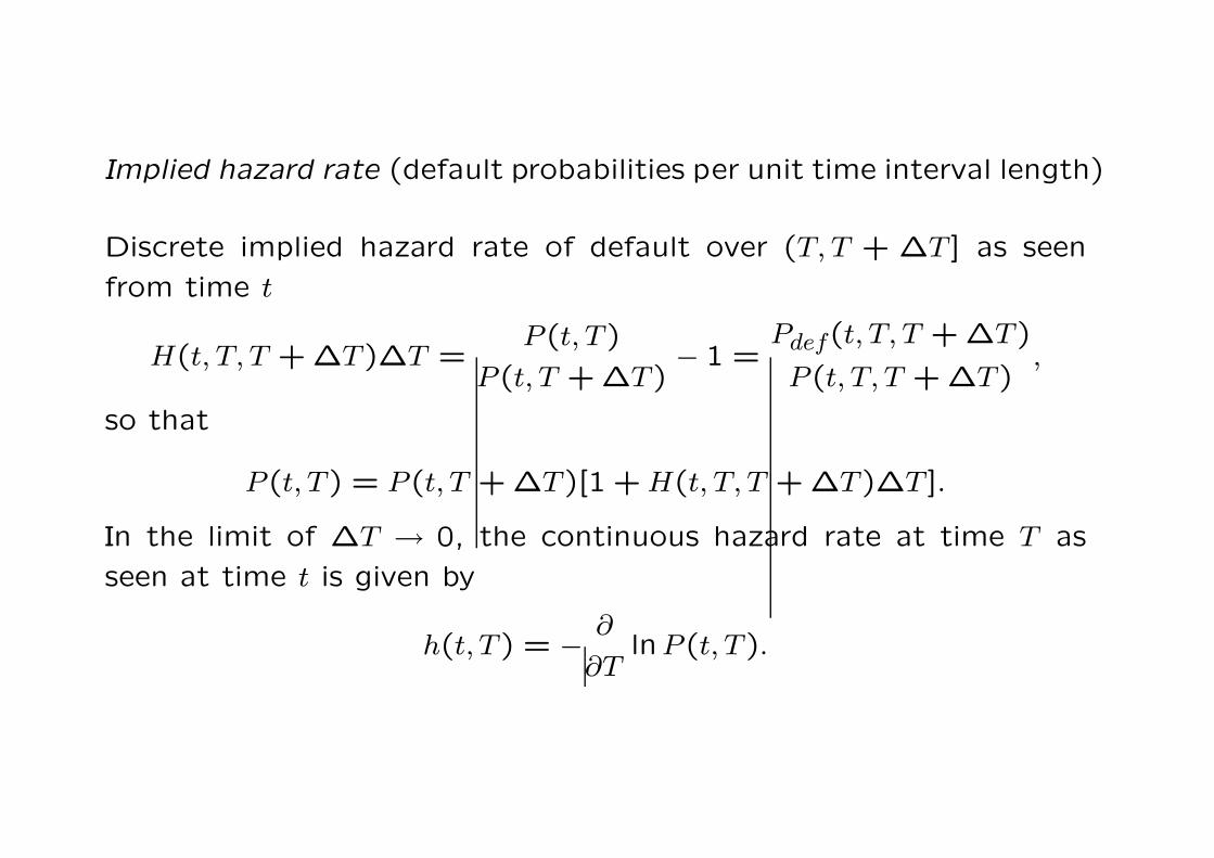
Implied hazard rate (default probabilities per unit time interval length)

Discrete implied hazard rate of default over (T, T + ∆T ] as seen

from time t

H(t, T, T + ∆T )∆T =P(t, T )

P(t, T + ∆T )− 1 =

Pdef(t, T, T + ∆T )

P(t, T, T + ∆T ),

so that

P(t, T ) = P(t, T + ∆T )[1 + H(t, T, T + ∆T )∆T ].

In the limit of ∆T → 0, the continuous hazard rate at time T as

seen at time t is given by

h(t, T ) = −∂

∂TlnP(t, T ).

Proof First, we recall

1

P(t, T, T + ∆T )=

P(t, T )

P(t, T, T + ∆T ).

We have

h(t, T ) = lim∆T→0

H(t, T, T + ∆T )

= lim∆T→0

1 − P(t, T, T + ∆T )

∆TP(t, T, T + ∆T )

= lim∆T→0

1

∆T

[P(t, T )

P(t, T + ∆T )− 1

]

= lim∆T→0

−1

P(t, T + ∆T )

P(t, T + ∆T ) − P(t, T )

∆T

= −1

P(t, T )

∂

∂TP(t, T )

= −∂

∂TlnP(t, T ).

Forward spreads and implied hazard rate of default

For t ≤ T1 < T2, the simply compounded forward rate over the

period (T1, T2] as seen from t is given by

F(t, T1, T2) =B(t, T1)/B(t, T2) − 1

T2 − T1.

This is the price of the forward contract with expiration date T1 on

a unit-par zero-coupon bond maturing on T2. To prove, we consider

the compounding of interest rates over successive time intervals.

1

B(t, T2)︸ ︷︷ ︸compounding over [t, T2]

=1

B(t, T1)︸ ︷︷ ︸compounding over [t, T1]

[1 + F(t, T1, T2)(T2 − T1)]︸ ︷︷ ︸simply compounding over [T1, T2]

Defaultable simply compounded forward rate over [T1, T2]

F(t, T1, T2) =B(t, T1)/B(t, T2) − 1

T2 − T1.

Instantaneous continuously compounded forward rates

f(t, T ) = lim∆T→0

F(t, T, T + ∆T ) = −∂

∂TlnB(t, T )

f(t, T ) = lim∆T→0

F(t, T, T + ∆T ) = −∂

∂TlnB(t, T ).

Implied hazard rate of default

Recall

P(t, T1, T2) =B(t, T2)

B(t, T2)

B(t, T1)

B(t, T1)

=1 + F(t, T1, T2)(T2 − T1)

1 + F(t, T1, T2)(T2 − T1)= 1 − Pdef(t, T1, T2),

and upon expanding, we obtain

Pdef(t, T1, T2) [1 + F(t, T1, T2)(T2 − T1)]︸ ︷︷ ︸B(t,T1)/B(t,T2)

= [F(t, T1, T2)−F(t, T1, T2)](T2−T1).

Define H(t, T1, T2) =Pdef(t, T1, T2)

(T2 − T1)P(t, T1, T2)as the discrete implied

rate of default. We then have

H(t, T1, T2) =B(t, T2)

B(t, T1)

[F(t, T1, T2) − F(t, T1, T2)]

P(t, T1, T2)

=B(t, T2)

B(t, T1)[F(t, T1, T2) − F(t, T1, T2)].

Taking the limit T2 → T1, then the implied hazard rate of default at

time T > t as seen from time t is the spread between the forward

rates:

h(t, T ) = f(t, T ) − f(t, T ).

Alternatively, we obtain the above relation using

f(t, T ) − f(t, T ) = −∂

∂Tln

B(t, T )

B(t, T )

= −∂

∂TlnP(t, T ) = h(t, T ).

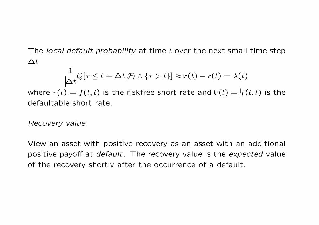
The local default probability at time t over the next small time step

∆t1

∆tQ[τ ≤ t + ∆t|Ft ∧ τ > t] ≈ r(t) − r(t) = λ(t)

where r(t) = f(t, t) is the riskfree short rate and r(t) = f(t, t) is the

defaultable short rate.

Recovery value

View an asset with positive recovery as an asset with an additional

positive payoff at default. The recovery value is the expected value

of the recovery shortly after the occurrence of a default.

Payment upon default

Define e(t, T, T +∆T ) to be the value at time t < T of a deterministic

payoff of $1 paid at T + ∆T if and only if a default happens in

[T, T + ∆T ].

e(t, T, T + ∆T ) = EQ [β(t, T + ∆T )[I(T ) − I(T + ∆T )]|Ft] .

Note that

I(T ) − I(T + ∆T ) =

1 if default occurs in [T, T + ∆T ]0 otherwise

,

EQ[β(t, T + ∆T )I(T )] = EQ[β(t, T + ∆T )]EQ[I(T )]

= B(t, T + ∆T )P(t, T ),

EQ[β(t, T + ∆T )I(T + ∆T )] = B(t, T + ∆T ),

and

B(t, T + ∆T ) = B(t, T + ∆T )/P (t, T + ∆T ).

It is seen that

e(t, T, T + ∆T ) = B(t, T + ∆T )P(t, T ) − B(t, T + ∆T )

= B(t, T + ∆T )

[P(t, T )

P(t, T + ∆T )− 1

]

= ∆TB(t, T + ∆T )H(t, T, T + ∆T )

On taking the limit ∆T → 0, we obtain

rate of default compensation = e(t, T ) = lim∆T→0

e(t, T, T + ∆T )

∆T= B(t, T )h(t, T ) = B(t, T )P(t, T )h(t, T ).

The value of a security that pays π(s) if a default occurs at time s

for all t < s < T is given by∫ T

tπ(s)e(t, s) ds =

∫ T

tπ(s)B(t, s)h(t, s) ds.

This result holds for deterministic recovery rates.

Random recovery value

• Suppose the payoff at default is not a deterministic function

π(τ) but a random variable π′ which is drawn at the time of

default τ . π′ is called a marked point process. Define

πe(t, T ) = EQ[π′|Ft ∧ τ = T].

which is the expected value of π′ conditional on default at T and

information at t.• Conditional on a default occurring at time T , the price of a

security that pays π′ at default is B(t, T )πe(t, T ).• Since the time of default is not known, we have to integrate

these values over all possible default times and weight them

with the respective probability of default occurring.• The price at time t of a payoff of π′ at τ if τ ∈ [t, T ] is given by

∫ T

tπe(t, s)B(t, s)P(t, s)︸ ︷︷ ︸

B(t,s)

h(t, s) ds.

Building blocks for credit derivatives pricing

Tenor structure

δk = Tk+1−Tk,0 ≤ k ≤ K−1

Coupon and repayment dates for bonds, fixing dates for rates, pay-

ment and settlement dates for credit derivatives all fall on Tk,0 ≤k ≤ K.

Fundamental quantities of the model

• Term structure of default-free interest rates F(0, T )• Term structure of implied hazard rates H(0, T )• Expected recovery rate π (rate of recovery as percentage of par)

From B(0, Ti) =B(0, Ti−1)

1 + δi−1F(0, Ti−1Ti), i = 1,2, · · · , k, and B(0, T0) =

B(0,0) = 1, we obtain

B(0, Tk) =k∏

i=1

1

1 + δi−1F(0, Ti−1, Ti).

Similarly, from P(0, Ti) =P(0, Ti−1)

1 + δi−1H(0, Ti−1, Ti), we deduce that

B(0, Tk) = B(0, Tk)P(0, Tk) = B(0, Tk)k∏

i=1

1

1 + δi−1H(0, Ti−1, Ti).

e(0, Tk, Tk+1) = δkH(0, Tk, Tk+1)B(0, Tk+1)

= value of $1 at Tk+1 if a default

has occurred in (Tk, Tk+1].

Taking the limit δi → 0, for all i = 0,1, · · · , k

B(0, Tk) = exp

(−∫ Tk

0f(0, s) ds

)

B(0, Tk) = exp

(−∫ Tk

0[h(0, s) + f(0, s)] ds

)

e(0, Tk) = h(0, Tk)B(0, Tk).

Alternatively, the above relations can be obtained by integrating

f(0, T ) = −∂

∂TlnB(0, T ) with B(0,0) = 1

f(0, T ) = h(0, T ) + f(0, T ) = −∂

∂TlnB(0, T ) with B(0,0) = 1.

Defaultable fixed coupon bond

c(0) =K∑

n=1

cnB(0, Tn) (coupon) cn = cδn−1

+ B(0, TK) (principal)

+ πK∑

k=1

e(0, Tk−1, Tk) (recovery)

The recovery payment can be written as

πK∑

k=1

e(0, Tk−1, Tk) =K∑

k=1

πδk−1H(0, Tk−1, Tk)B(0, Tk).

The recovery payments can be considered as an additional coupon

payment stream of πδk−1H(0, Tk−1, Tk).

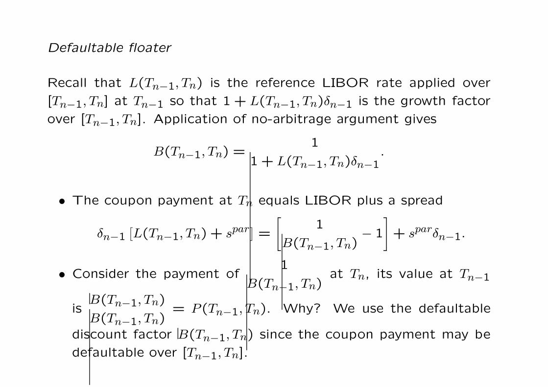
Defaultable floater

Recall that L(Tn−1, Tn) is the reference LIBOR rate applied over

[Tn−1, Tn] at Tn−1 so that 1 + L(Tn−1, Tn)δn−1 is the growth factor

over [Tn−1, Tn]. Application of no-arbitrage argument gives

B(Tn−1, Tn) =1

1 + L(Tn−1, Tn)δn−1.

• The coupon payment at Tn equals LIBOR plus a spread

δn−1[L(Tn−1, Tn) + spar] =

[1

B(Tn−1, Tn)− 1

]+ sparδn−1.

• Consider the payment of1

B(Tn−1, Tn)at Tn, its value at Tn−1

isB(Tn−1, Tn)

B(Tn−1, Tn)= P(Tn−1, Tn). Why? We use the defaultable

discount factor B(Tn−1, Tn) since the coupon payment may be

defaultable over [Tn−1, Tn].

• Seen at t = 0, the value becomes

B(0, Tn−1)P(0, Tn−1, Tn)

= B(0, Tn−1)P(0, Tn−1)P(0, Tn−1, Tn)

= B(0, Tn−1)P(0, Tn).

Combining with the fixed part of the coupon payment and observing

the relation

[B(0, Tn−1) − B(0, Tn)]P(0, Tn) =

[B(0, Tn−1)

B(0, Tn)− 1

]B(0, Tn)

= δn−1F(0, Tn−1, Tn)B(0, Tn),

the model price of the defaultable floating rate bond is

c(0) =K∑

n=1

δn−1F(0, Tn−1, Tn)B(0, Tn) + sparK∑

n=1

δn−1B(0, Tn)

+ B(0, TK) + πK∑

k=1

e(0, Tk−1, Tk).

Credit default swapFixed leg Payment of δn−1s at Tn if no default until Tn.

The value of the fixed leg is

sN∑

n=1

δn−1B(0, Tn).

Floating leg Payment of 1 − π at Tn if default in (Tn−1, Tn]

occurs. The value of the floating leg is

(1 − π)N∑

n=1

e(0, Tn−1, Tn)

= (1 − π)N∑

n=1

δn−1H(0, Tn−1, Tn)B(0, Tn).

The market CDS spread is chosen such that the fixed leg and float-

ing leg of the CDS have the same value. Hence

s = (1 − π)

N∑

n=1

δn−1H(0, Tn−1, Tn)B(0, Tn)

∑Nn=1 δn−1B(0, Tn)

.

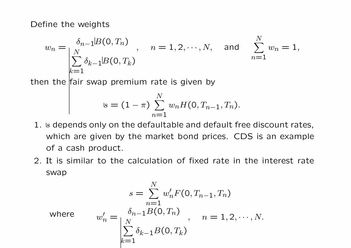
Define the weights

wn =δn−1B(0, Tn)

N∑

k=1

δk−1B(0, Tk)

, n = 1,2, · · · , N, andN∑

n=1

wn = 1,

then the fair swap premium rate is given by

s = (1 − π)N∑

n=1

wnH(0, Tn−1, Tn).

1. s depends only on the defaultable and default free discount rates,

which are given by the market bond prices. CDS is an example

of a cash product.

2. It is similar to the calculation of fixed rate in the interest rate

swap

s =N∑

n=1

w′nF(0, Tn−1, Tn)

where w′n =

δn−1B(0, Tn)N∑

k=1

δk−1B(0, Tk)

, n = 1,2, · · · , N.

Marked-to-market value

original CDS spread = s′; new CDS spread = s

Let Π = CDSold − CDSnew, and observe that CDSnew = 0, then

marked-to-market value = CDSold = Π = (s − s′)N∑

n=1

B(0, Tn)δn−1.

Why? If an offsetting trade is entered at the current CDS rate s,

only the fee difference (s − s′) will be received over the life of the

CDS. Should a default occurs, the protection payments will cancel

out, and the fee difference payment will be cancelled, too. The

fee difference stream is defaultable and must be discounted with

B(0, Tn).

• CDS’s are useful instruments to gain exposure against spread

movements, not just against default arrival risk.

Valuing credit default swap I: No counterparty default risk

by John Hull and Alan White, Journal of Derivatives (Fall 2000)

p.29-40.

• Estimation of the risk neutral probability that the reference bond

will default at different times in the future. The market prices of

bonds issued by the same obligor and Treasury bonds are used

to provide the market information of the expected default loss

of the reference entity.

– Choose a set of N bonds issued by the obligor with maturity

dates tj, j = 1,2, · · · , N , where tj−1 < tj and t = 0. The life of

CDS is [0, tN ].

Bj = market price of Treasury bond with maturity date tj

Bj = market price of defaultable bond with maturity date tj

Bj − Bj gives the market estimation of the present value of

expected default loss of the jth defaultable bond over the period

[0, tj], j = 1,2, · · · , N .

Assume the risk neutral default probability density function q(t) to be

piecewise constant over [0, tN ], q(t) = qi, t ∈ (ti−1, ti], i = 1,2, · · · , N .

Define βij be the present value of the expected default loss of the

jth risky bond defaulting within (ti−1, ti], i ≤ j. We deduce that

j∑

i=1

qiβij = Bj − Bj, j = 1,2, · · · , N. (i)

Try to determine qi by estimating βij.

Assumptions

1. We estimate the expected recovery rate from historical data.

2. We assume that all risky bonds have the same seniority and

the expected recovery rate is time independent. Let R be this

expected recovery rate, which is independent of j and t.

3. Let Cj(t) denote the claim amount on the jth bond defaulting

at time t, then

Cj(t) = L[1 + A(t)],

L = face value, A(t) = accrued interest at time t as percentage

of its face value.

4. The protection buyer has to pay at default the accrued pay-

ment covering the period between the default time and the last

payment date.

5. The default event, Treasury interest rates and recovery rates

are mutually independent (under the risk neutral measure).

6. From the riskless Treasury interest rate, we can compute the

discount factor v(t), which is the present value of $1 received

at time t with certainty.

Let Fj(t) be the forward price of the jth default-free bond for a for-

ward contract maturing at time t. Assuming deterministic interest

rate, then the price at time t of the no-default value of the jth bond

is Fj(t). We then have

βij =∫ ti

ti−1

v(t)[Fj(t) − RCj(t)

]dt i ≤ j, j = 1,2, · · · , N. (ii)

From Eq. (i), we can deduce

qj =Bj − Bj −

∑j−1i=1 qiβij

βjj, j = 1,2, · · · , N. (iii)

The risk neutral expected payoff paid by the protection seller upon

default at time t is L1− R[1+A(t)]. Therefore, the present value

of the expected payoff is∫ T

0L1 − R[1 + A(t)]q(t)v(t) dt.

Greatest weakness of the model The computation of βij requires the

information of the bond prices at time t. By imposing non-stochastic

property of the interest rate, the bond prices at future time t equals

the current traded bond forward price Fj(t). Since CDS is a cash

product, it should be priced purely based on defaultable and default

free discount rates without any assumption on the stochastic nature

of the interest rate.

How to compute the annuity premium rate w paid by the protection

buyer?

u(t) = present value of payments at the rate of $1 per year on payment

dates between time zero and t

e(t) = present value of an accrual payment at time t of the time interval

t − t∗, where t∗ is the last payment date.

If there is no default prior to CDS maturity, the present value of

payments is wu(T ).

Expected value of payments

= w∫ T

0Lq(t)[u(t) + e(t)] dt + wLu(T )

[1 −

∫ T

0q(t) dt

].

Lastly, w is determined such that the present value of payments

equals the present value of expected default loss. Hence

w =

∫ T0 1 − R[1 + A(t)]q(t)v(t) dt

∫ T0 q(t)[u(t) + e(t)] dt + u(T )

[1 −

∫ T0 q(t) dt

].

Hedge based pricing – approximate hedge and replication strate-

gies

Provide hedge strategies that cover much of the risks involved in

credit derivatives – independent of any specific pricing model.

Basic instruments

1. Default free bond

C(t) = time-t price of default-free bond with fixed-coupon C

B(t, T ) = time-t price of default-free zero-coupon bond

2. Defaultable bond

C(t) = time-t price of defaultable bond with fixed-coupon c

C ′(t) = time-t price of defaultable bond with floating coupon

LIBOR + spar

3. Interest rate swap

S(t) = swap rate at time t of a standard fixed-for-floating

=B(t, tn) − B(t, tN)

A(t; tn, tN), t ≤ tn

where A(t; tn, tN) =N∑

i=n+1

δiB(t, ti) = value of the payment stream

paying δi on each date ti.

Proof of the swap rate formula

The floating rate coupon payments can be generated by putting $1

at tn and taking away the floating interests immediately. At tN ,

$1 remains. The sum of the present value of the floating interests

= B(t, tn) − B(t, tN).

Intuition behind cash-and-carry arbitrage pricing of CDSs

A combined position of a CDS with a defaultable bond C is very

well hedged against default risk.

Hedge strategy using fixed-coupon bonds

Portfolio 1

• One defaultable coupon bond C; coupon c, maturity tN .• One CDS on this bond, with CDS spread s

The portfolio is unwound after a default.

Portfolio 2

• One default-free coupon bond C: with the same payment dates

as the defaultable coupon bond and coupon size c − s.

The bond is sold after default.

Observations

1. In survival, the cash flows of both portfolio are identical.

Portfolio 1 Portfolio 2t = 0 −C(0) −C(0)t = ti c − s c − st = tN 1 + c − s 1 + c − s

2. At default, portfolio 1’s value = par = 1 (full compensation by

CDS); that of portfolio 2 is C(τ), τ is the time of default.

The price difference at default = 1 − C(τ). This difference is

very small when the default-free bond is a par bond. “The issuer

can choose c to make the bond be a par bond.”

This is an approximate replication. Neglecting the price difference

at default, the no-arbitrage principle dictates

C(0) = C(0) = B(0, tN) + cA(0) − sA(0).

The equilibrium CDS rate s can be solved. C(0) and C(0) have

almost the same value when the defaultable bond pays less coupon

of amount equals the spread s.

Cash-and carry arbitrage with par floater

A par floater C ′ is a defaultable bond with a floating-rate coupon

of ci = Li−1 + spar, where the par spread spar is adjusted such that

at issuance the par floater is valued at par.

Portfolio 1

• One defaultable par floater C ′ with spread spar over LIBOR.• One CDS on this bond: CDS spread is s.

The portfolio is unwound after default.

Portfolio 2

• One default-free floating-coupon bond C ′: with the same pay-

ment dates as the defaultable par floater and coupon at LIBOR,

ci = Li−1.

The bond is sold after default.

Time Portfolio 1 Portfolio 2t = 0 −1 −1t = ti Li−1 + spar − s Li−1t = tN 1 + LN−1 + spar − s 1 + LN−1τ (default) 1 C ′(τ) = 1 + Li(τ − ti)

The hedge error in the payoff at default is caused by accrued inter-

est. If we neglect the small hedge error at default, then

spar = s.

Asset swap packages

An asset swap package consists of a defaultable coupon bond C with

coupon c and an interest rate swap. The bond’s coupon is swapped

into LIBOR plus the asset swap rate sA. Asset swap package is sold

at par.

Remark Asset swap transactions are driven by the desire to strip

out unwanted structured features from the underlying asset.

Payoff streams to the buyer of the asset swap package

time defaultable bond swap nett = 0 −C(0) −1 + C(0) −1t = ti c∗ −c + Li−1 + sA Li−1 + sA + (c∗ − c)t = tN (1 + c)∗ −c + LN−1 + sA 1∗ + LN−1 + sA + (c∗ − c)default recovery unaffected recovery

* denotes payment contingent on survival.

s(0) = fixed-for-floating swap rate (market quote)

A(0) = value of an annuity paying at the $1 (calculated based on

observable default free bond prices)

The value of asset swap package is set at par at t = 0, so thatC(0) + A(0)s(0) + A(0)sA(0) − A(0)c︸ ︷︷ ︸

swap arrangement

= 1.

The present value of the floating coupons is given by A(0)s(0). The

swap continues even after default so that A(0) appears in all terms

associated with the swap arrangement. Solving for sA(0)

sA(0) =1

A(0)[1 − C(0)] + c − s(0).

Rearranging the terms,

C(0) + A(0)sA(0) = [1 − A(0)s(0)] + A(0)c︸ ︷︷ ︸default-free bond

≡ C(0)

where the right-hand side gives the value of a default-free bond with

coupon c. Note that 1 − A(0)s(0) is the present value of receiving

$1 at maturity tN . We obtain

sA(0) =1

A(0)[C(0) − C(0)].

Credit spread options

The terminal payoff is given by

Psp(r, s, T ) = max(s − K,0)

where r = riskless interest rate

s = credit spread

K = strike spread

Discrete-time Heath-Jarrow-Morton (HJM) method (Das and Sun-

daram, 2000)

• Follows the HJM term structure approach that models the for-

ward rate process and forward spread process for riskless and

risky bonds.• The model takes the observed term structures of riskfree forward

rates and credit spreads as input information.• Find the risk neutral drifts of the stochastic processes such that

all discounted security prices are martingales.

Example Price a one-year put spread option on a two-year risky

zero-coupon bond struck at the strike spread K = 0.01.

Let the current observed term structure of riskless interest rates as

obtained from the spot rate curve for Treasury bonds be

r =

(0.070.08

).

The riskless forward rate between year one and year two is

f12 =1.082

1.07− 1 ≈ 0.09.

The market one-year and two-year spot spreads are

s =

(0.0100.012

).

The two-year risky rate is 0.08 + 0.012 = 0.092. The current price

of a risky two-year zero coupon bond with face value $100 is

B(0) = $100/(1.092)2 = $83.86.

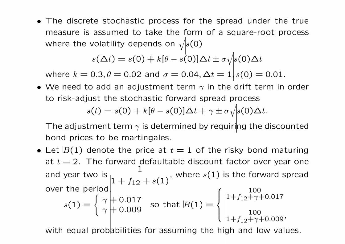
• The discrete stochastic process for the spread under the true

measure is assumed to take the form of a square-root process

where the volatility depends on√

s(0)

s(∆t) = s(0) + k[θ − s(0)]∆t ± σ√

s(0)∆t

where k = 0.3, θ = 0.02 and σ = 0.04,∆t = 1, s(0) = 0.01.

• We need to add an adjustment term γ in the drift term in order

to risk-adjust the stochastic forward spread process

s(t) = s(0) + k[θ − s(0)]∆t + γ ± σ√

s(0)∆t.

The adjustment term γ is determined by requiring the discounted

bond prices to be martingales.

• Let B(1) denote the price at t = 1 of the risky bond maturing

at t = 2. The forward defaultable discount factor over year one

and year two is1

1 + f12 + s(1), where s(1) is the forward spread

over the period.

s(1) =

γ + 0.017γ + 0.009

so that B(1) =

1001+f12+γ+0.017

1001+f12+γ+0.009,

with equal probabilities for assuming the high and low values.

We determine γ such that the bond price is a martingale.

B(0) = 83.86 =1

1 + 0.07 + 0.01×

1

2

(100

1.107 + γ+

100

1.099 + γ

).

The first term is the risky defaultable discount factor and the last

term is the expected value of B(1). We obtain γ = 0.0012 so that

s(1) =

0.01820.0102

.

The current value of put spread option is

1

1.07×

1

2[(0.0182 − 0.01) + (0.0102 − 0.01)]L = 0.00393L,

where L is the notional value of the put spread option. Note that

the default free discount factor 1/1.07 is used in the option value

calculation.

Two-factor Hull-White “no-arbitrage” model

Under the risk neutral measure Q, the stochastic processes followed

by the short rate r and the short spread rate s are

dr = [φ(t) − αr] dt + σr dZr

ds = [θ(t) − βs] dt + σs dZs,

where φ(t) and θ(t) are time dependent parameter functions, α and

β are mean reversion parameters, dZr dZs = ρ dt. The sum r(t)+s(t)

is considered as the risky short rate.

• “No-arbitrage” refers to the determination of the time depen-

dent drift terms in the mean reversion stochastic processes of r

and s by fitting the current term structures of default free and

defaultable bond prices. This is a calibration procedure.

B(t, T ) = EQ

[exp

(−∫ T

tr(u) du

)]

B(t, T ) = EQ

[exp

(−∫ T

t[r(u) + s(u)] du

)].

B(r, t;T ) admits solution of the form a(r, t;T )e−rb(r,t;T ). The process

followed by B(t, T ) is given by

dB

B= r dt + σB(t, T ) dZr

where

σB(t, T ) = −σr

α[1 − e−α(T−t)].

In terms of the forward measure QT where B(t, T ) is used as the

numeraire, the defaultable bond price is

B(t, T ) = B(t, T )EQT

[exp

(−∫ T

ts(u) du

)].

In general,V (t)

B(t, T )= EQT

[V (T )

B(T, T )

]so that V (t) = B(t, T )EQT [V (T )].

The process followed by the credit spread s under QT is given by

ds = [θ(t) − βs + ρσsσB(t, T )] dt + σs dZT

where ZT is the standard Wiener process under QT .

The stochastic quantity∫ T

ts(u) du has

mean = EQT

[∫ T

ts(u) du

]=

s(t)

β[1 − e−β(T−t)]

+∫ T

t[θ(u) + ρσsσB(u, T )]

1 − e−β(T−u)

βdu

variance = var

(∫ T

ts(u) du

)=

∫ T

t

σ2s

β2

[1 − e−β(T−u)

]2du.

Hence,

B(t, T )

B(t, T )= EQT

[exp

(−∫ T

ts(u) du

)]

= exp

(−

s(t)σs

β[1 − e−β(T−t)]

)

−∫ T

t[θ(u) + ρσsσB(u, T )]

1 − e−β(T−u)

βdu

+∫ T

t

σ2s

2β2[1 − e−β(T−u)]2 du.

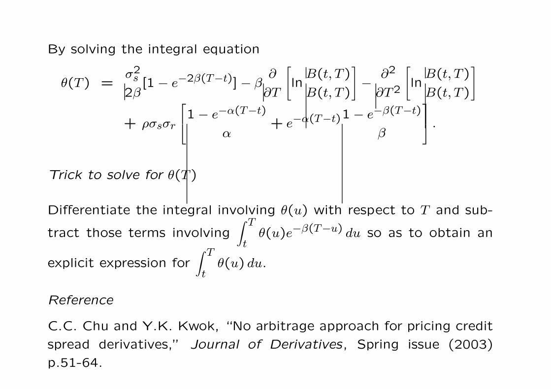
By solving the integral equation

θ(T ) =σ2

s

2β[1 − e−2β(T−t)] − β

∂

∂T

[ln

B(t, T )

B(t, T )

]−

∂2

∂T2

[ln

B(t, T )

B(t, T )

]

+ ρσsσr

1 − e−α(T−t)

α+ e−α(T−t)1 − e−β(T−t)

β

.

Trick to solve for θ(T )

Differentiate the integral involving θ(u) with respect to T and sub-

tract those terms involving∫ T

tθ(u)e−β(T−u) du so as to obtain an

explicit expression for∫ T

tθ(u) du.

Reference

C.C. Chu and Y.K. Kwok, “No arbitrage approach for pricing credit

spread derivatives,” Journal of Derivatives, Spring issue (2003)

p.51-64.

Pricing of the credit spread option

psp(r, s, t) = B(t, T )EQT [max(s − K,0)].

Note the presence of the mean reversion term −βs in the drift term.

Define

ξ(t) = e−β(T−t)s(t)

so that

dξ = [θ(t) + ρσsσB(t, T )][−β(T − t)] dt + σs[−β(T − t)] dZT .

Now, ξT is normally distributed with mean µξ and σ2ξ , where

µξ = s(t)e−β(T−t) +ρσsσr

α

1 − e−(α+β)(T−t)

α + β−

1 − e−β(T−t)

β

+∫ T

tθ(u)e−β(T−u) du

andσ2

ξ =σ2

s

2β[1 − e2β(T−t)].

Spread option value

psp(r, s, t) = B(r, t)

[σξ√2π

e−(K−µξ)2/2σ2

s + (µξ − K)N

(µξ − K

σξ

)].