§1.2 Functions & Function Notation - Yvette Butterworth · Y. Butterworth Ch. 1 Notes to Accompany...

Y. Butterworth Ch. 1 Notes to Accompany Functions Modeling Change, of 12 Connally, Hughes-Hallett, Gleason, et al, 3rd Edition Connally, Hughes-Hallett, Gleason, et al, 3rd Edition

§1.2 Functions & Function Notation A relation is any set of ordered pairs. A function is a relation for which every value of the independent variable (the values that can be inputted; the t’s; used to call the x’s) has one and only one value for the dependent variable (the values that are output, dependent upon those input; the Q’s; used to call the y’s). All the possible values of the independent variable form the domain and the values given by the dependent variable form the range. Think of a function as a machine and once a value is input it becomes something else, thus you can never input the same thing twice and have it come out differently. This does not mean that you can't input different things and have them come out the same, however! That is another discussion for a later time (that’s called a function being one-to-one). Ways to Represent Functions: 1) Description in words Example: The average population of a city from the turn of the 20th century to present day. 2) Tables Example: See below 3) Graphs Example: 4) Formulas Example: Q(t) = 2x + 1 Is a the set of ordered pairs a function? 1) For every value in the domain is there only one value in the range? a) Looking at ordered pairs – If no x’s repeat then it’s a function (a map can be used to see this too. Domain on left & range on right, If any domain value has lines to more than one range value, then not a function.) b) Looking at a graph – Vertical line test (if any vertical line intersects the graph in more

than one place the relation is not a function) c) Mathematical Model needs to consider the domain & range values or draw a picture– If input of any x will give different y’s, then not a function (probably a graph is still best!) d) From a description – Try to model using a set of ordered pairs, a graph or a model to decide if it is a function. There are many ways to show a function. We can describe the function in words, draw a graph, list the domain and range values using set notation such as roster form or we can make a table of values, or we can use a mathematical model (an equation) to describe the function.

x 5 -5

5

-5

These are tables. Left is f(n) Rt. Is not an f(n)

x 1 2 3 f(x) 2.3 2.8 3.2 *(#11 p. 5 Applied Calculus, Hughes-Hallett et al, 4th Edition, Wiley, 2010)

x 1 1 2 f(x) 2.3 2.8 3.2


Although I won’t give you an example that isn’t a function, here an example in words that is a function. We’ll investigate it by sketching a graph. IS: A patient experiencing rapid heart is administered a drug which causes the patient’s heart rate to plunge dramatically and as the drug wears off, the patient’s heart rate begins to slowly rise. Function notation may have been discussed in algebra, but if it wasn't you didn't miss much. It is just a way of describing the dependent variable as a function of the independent. It is written using any letter, usually f or g and in parentheses the independent variable. This notation replaces the dependent variable, y.

f (x) Read as f of x The notation means evaluate the equation at the value given within the parentheses. It is exactly like saying y=!! Example: The population of a city, P, in millions is a function t, the number of years since 1970, so P = f(t). Explain the meaning of the statement f(35) = 12 in terms of the population of the city.(#2 p.5 Applied Calculus, Hughes-Hallett et al, 4th Edition, Wiley, 2010)

2 3 5

15 25 2

5 6 7

These are maps. Left is f(n) Rt. Is not an f(n)

^ ^

x

y

15 -15 5

-5

These are graphs. Left is f(n) Rt. Is not an f(n)

These are models. Left is f(n) Rt. Is not an f(n)

y = 10x – x2 (#8 p. 5 Applied Calculus, Hughes-

Hallett et al, 4th Edition, Wiley, 2010)

y2 + x2 = 9


Example: Find the value of f(5) a) f(x) = 2x + 3 b) c) *(#10 p.5 Applied Calculus, Hughes-Hallett et al, 4th Edition, Wiley, 2010)

Function notation can also be used to solve equations. Example: Find all values of x for which f(x) = 25 if f(x) = x2 + 9 The following example shows how we can model a real life situation with a formula using 3 parameters (numbers that are subject to change), but once one parameter is firmly defined we create a linear function and then that function can be represented using function notation. Function notation gives some indication of the meaning of the independent and dependent variables. A graph of the function can be used visualize the relationship between the independent and dependent variables. Example: The perimeter of a rectangle is P = 2L + 2w. If it is

known that the length must be 10 feet, then the perimeter is a function of width.

a) Write this function using function notation b) Find the perimeter given the width is 2 ft. Write this

using function notation. c) Use your graphing calculator to graph the function which shows the relationship between the length of the rectangle and the perimeter.

x 1 3 5 7 f(x) 9 12 15 18


d) Use your calculator to find 3 sets of ordered pairs, writing those in a table here. e) What do you notice happening to P(L) as L gets larger? What do you notice about the graph at L gets larger? This shows the concept of an increasing function – as the values of the independent increase so do the values of the independent. *Note: We will see the decreasing function exhibited in an example for the next section. In this last example, the perimeter formula that we are familiar with from Algebra is called a mathematical model. We will be creating mathematical models of our own and representing them using function notation. Example: A chemical company spends $2 million to buy machinery before it starts producing chemicals. Then it spends $0.5 million on raw materials for each million liters of chemical produced. (Adapted from #34 p. 9, Functions Modeling Change, Connally, Hughes-Hallet, Gleason, et al,Ed 3) a) Is cost a function of millions of liters or is millions of liters a function of cost? b) Define the independent variable & the dependent variable. c) Using a function notation write a mathematical model for this scenario. Here is some additional material that might help fill in the blanks: Building a mathematical model of a situation that has a linear relationship requires knowledge of the slope and the vertical intercept. There are 2 ways to build the mathematical model given just two ordered pairs (two pieces of information relating the independent and dependent variables in two instances). We can use both the slope-intercept and the point-slope forms of a line to model data. To use the slope-intercept, we must know the base-line value (the value of the dependent when the independent is zero; the vertical intercept). We don’t need the base-line if we use the point-slope form of a line to model. Point-Slope Form y − y0 = m(x − x0) m = slope

(x0, y0) is a point on the line x & y are variables (don’t substitute for those)


Now, let’s use the two functional forms of a linear equation in two variables to find mathematical models for our two situations given above as slope problems. Example: Find the equation of the lines described a) Through the points *(i) is #8 p.12 & ii) is #6p.12 Applied Calculus, Hughes-Hallett et al, 4th Edition, Wiley, 2010) i) (4, 5) & (2, -1) ii) (0, 0) & (1, 1) b) Shown on the graph But of course this is not how’ll we be using it in this class. We want to do applications. For this we will borrow some applications from Economics found in section 4. We will be using the cost function, C(q), which is the total cost for quantity, q, of some good and the revenue function, R(q), which gives the total revenue received by a firm for selling a quantity, q, of some good and the profit function, π, given by R(q) – C(q). Example: A company that makes jigsaw puzzles has fixed costs of $6000 plus each puzzle costs $2 per puzzle to make (the variable cost). The company sells each puzzle for $5 each.*(#14p.36 Applied Calculus, Hughes-Hallett et al, 4th Edition, Wiley, 2010) a) Find the cost function (fixed costs are base-line amounts). b) Find revenue function. Example: Use the following table of to find the cost function.*(#12p.36 Applied Calculus, Hughes-Hallett et al, 4th Edition, Wiley, 2010) a) Using slope or vertical or horizontal intercept, which describes the fixed cost (cost to produce goods regardless of cost per item)? What is the fixed cost? b) Using slope or vertical or horizontal intercept, which describes the cost to produce an item (the marginal cost)? What is the marginal cost? c) Give the cost function.

q 0 5 10 15 20 C(q) 5000 5020 5040 5060 5080

x

y


Example: Based on the figure below, answer the following questions.*(#3p.35 Applied Calculus, Hughes-Hallett et al, 4th Edition, Wiley, 2010)

c) Using your estimate from a and your answer to b), what do you believe the marginal cost to be? d) In relation to a line, what quantity does the marginal cost represent? e) Give a cost function for this graph based upon the answers from the above questions? This discussion leads naturally into section 1.4 material, so we will cover that section next, and since we have already started, there is no time like the present. Break-even points are the point of intersection of a cost and a revenue function. The break-even point represents the quantity at which the revenue and the cost are equal and thus the profit is zero (recall that profit, π, is R(q) – C(q)). Recall from algebra that the intersection of two functions is where the independent and dependent value for both functions are identical. This point can be found mathematically or visually. Visually, we see the point of intersection of the functions’ graphs and can read the values of the independent and dependent from the graph itself. Mathematically we can solve the system by setting the two functions equal and solving for the one variable (in the case of function notation we are solving for the independent value – in our case the quantity, q). Let’s review the visual method using our calculators. Method #1: Intersection of Equations (the solution of a system) 1) Graph each function 2) Find the intersection of the functions 3) The x-coordinate of the point of intersection is the quantity. This is the quantity at which the company will break even. The y-coordinate is the C(q) or the R(q), since it is the amount of money where C(q)=R(q) or where π(q)=0.

a) Estimate the fixed cost of producing goods. b) What is C(10)? What does this represent?


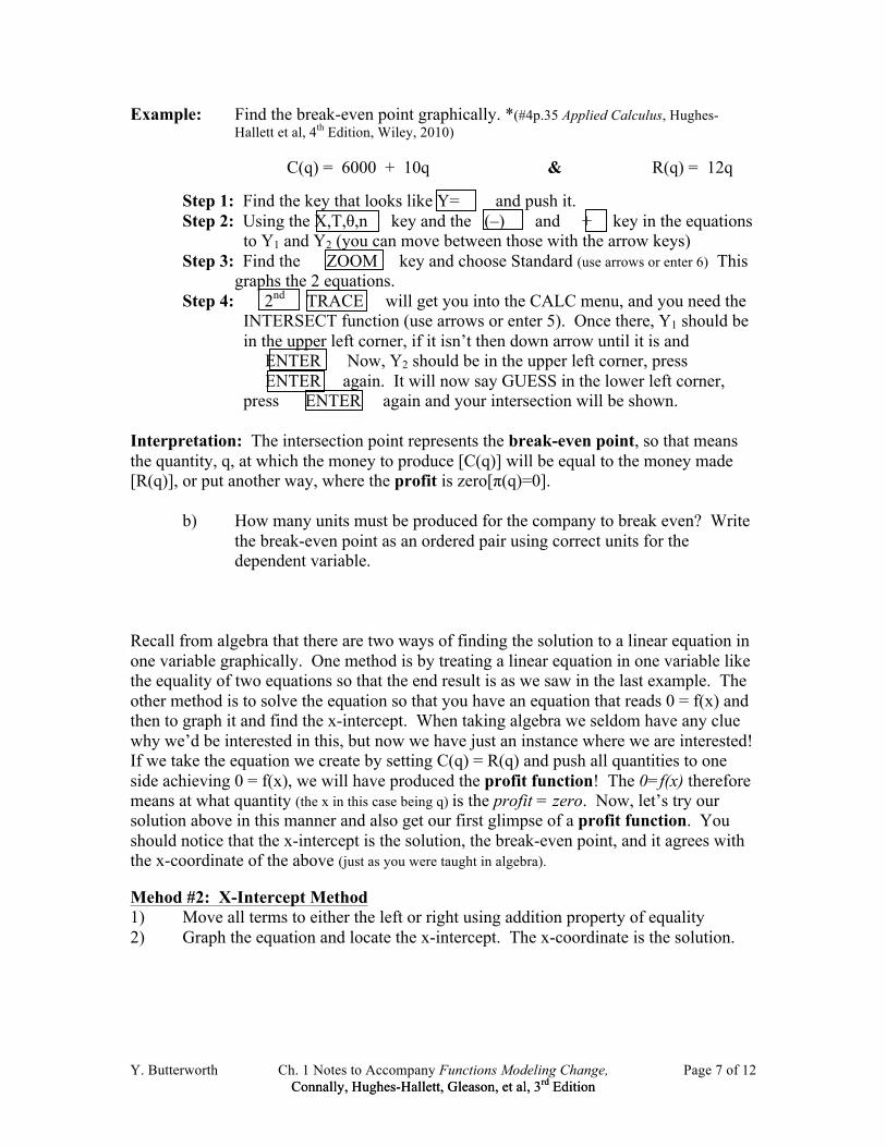
Example: Find the break-even point graphically. *(#4p.35 Applied Calculus, Hughes- Hallett et al, 4th Edition, Wiley, 2010) C(q) = 6000 + 10q & R(q) = 12q Step 1: Find the key that looks like Y= and push it. Step 2: Using the X,T,θ,n key and the (–) and + key in the equations to Y1 and Y2 (you can move between those with the arrow keys) Step 3: Find the ZOOM key and choose Standard (use arrows or enter 6) This graphs the 2 equations. Step 4: 2nd TRACE will get you into the CALC menu, and you need the INTERSECT function (use arrows or enter 5). Once there, Y1 should be in the upper left corner, if it isn’t then down arrow until it is and ENTER Now, Y2 should be in the upper left corner, press ENTER again. It will now say GUESS in the lower left corner, press ENTER again and your intersection will be shown. Interpretation: The intersection point represents the break-even point, so that means the quantity, q, at which the money to produce [C(q)] will be equal to the money made [R(q)], or put another way, where the profit is zero[π(q)=0]. b) How many units must be produced for the company to break even? Write the break-even point as an ordered pair using correct units for the dependent variable. Recall from algebra that there are two ways of finding the solution to a linear equation in one variable graphically. One method is by treating a linear equation in one variable like the equality of two equations so that the end result is as we saw in the last example. The other method is to solve the equation so that you have an equation that reads 0 = f(x) and then to graph it and find the x-intercept. When taking algebra we seldom have any clue why we’d be interested in this, but now we have just an instance where we are interested! If we take the equation we create by setting C(q) = R(q) and push all quantities to one side achieving 0 = f(x), we will have produced the profit function! The 0=f(x) therefore means at what quantity (the x in this case being q) is the profit = zero. Now, let’s try our solution above in this manner and also get our first glimpse of a profit function. You should notice that the x-intercept is the solution, the break-even point, and it agrees with the x-coordinate of the above (just as you were taught in algebra). Mehod #2: X-Intercept Method 1) Move all terms to either the left or right using addition property of equality 2) Graph the equation and locate the x-intercept. The x-coordinate is the solution.


Example: Give the profit function and quantity produced at which the company will break even using the x-intercept method. Use the same C(q) & R(q) from above. Step 1: Set C(q)=R(q) and push all terms to one side so you attain 0 = f(q Step 2: Again graph the equation. Note: If there are other equations in your calculator you can prevent them from being graphed by moving your cursor to the equal sign (use the arrow keys) and pressing ENTER The equal signs will be un- highlighted, meaning that they won’t be graphed. Step 3: Again go to the CALCULATE menu (see the above) and this time choose the ZERO (use the arrow keys or press 2). The calculator will prompt LOWER BOUND? in the lower left corner and you should press ENTER Now it (use the up/down arrow key) to move the cursor along the line until it is on the other side of the x-intercept, and press ENTER again. Now it will prompt you with GUESS? in the lower left corner and you will press ENTER again and be rewarded with the x-intercept. §1.2 Rate of Change Here is some review material for you about linear equations in 2 variables: Linear Equation in Two Variable is an equation in the following form, whose solutions are ordered pairs. A straight line can graphically represent a linear equation in two variables. As long as we are not talking about a vertical line (x = any #), all linear equations are functions.

ax + by = c a, b, & c are constants x, y are variables x & y both can’t = 0 Also Recall from Beginning Algebra: Solving an equation for y is called putting it in slope-intercept form. This is a special form, the functional form of the linear equation in two variables, which has the following properties. y = mx + b m = slope

b = y-intercept The other great thing about this form is that it allows us to use function notation and eliminate the need to write the dependent variable. Hence, y = mx + b becomes f(x) = mx + b since y is a function of x.

} Parameters


An intercept is where a graph crosses an axis (any graph, including those of linear functions have intercepts). There are two types of intercepts for any graph, a horizontal intercept (x-intercept;zeros) and a vertical intercept (y-intercept). A horizontal intercept is where the graph crosses the x-axis and it has an ordered pair of the form (x, 0). In terms of a function it describes at what value of the independent variable, the dependent variable reaches a value of zero. A vertical intercept is where the graph crosses the y-axis and it has an ordered pair of the form (0, y) most often written (0, b). In terms of a function it describes what the “base-line” value of the situation is. In other words, it gives the value of the dependent variable when the independent is zero. Finding the Y-intercept (X-intercept) Step 1: Let x = 0 (for x-intercept let y = 0) Step 2: Solve the equation for y (solve for x to find the x-intercept) Step 3: Form the ordered pair (0,y) where y is the solution from step two. [the ordered

pair would be (x, 0)] The actual heart of this section: Slope is the ratio of vertical change to horizontal change for a linear equation in two variables. It is the rate of change of the dependent variable per unit of the independent. The last iteration of the slope presented here is referred to as the difference quotient (it is the same as the familiar y2 – y1 over x2 – x1 except it uses function notation). m = rise = y2 − y1 = Δy = f(x2) – f(x1) run x2 − x1 Δx x2 – x1 The difference quotient can also be said to represent the average rate of change of a function from point a to point b. This allows us to take what we know from linear functions and apply it ANY function. Keep in mind that not all functions have a constant rate of change as a linear function does. Essentially what we are doing is creating a line between two points on a curve that tells us about the average rate of change on an interval (this is what a secant line is btw). Ave. Rate of Change = f(b) – f(a) = ∆y for t = b and t = a b – a ∆t when y = f(t)

3Ways to Find Slope 1) Formula given above Example: Use the formula to find the slope of the line through a) (4, 5) & (2, -1) b) (0, 0) & (1, 1)

Y. Butterworth Ch. 1 Notes to Accompany Functions Modeling Change, of 12 Connally, Hughes-Hallett, Gleason, et al, 3rd Edition

2) Geometrically using m = rise/run Choose points, create rise & run triangle, count & divide Example: Find the slope of the line given. 3) From the slope-intercept form of a linear function y = mx + b, where m, the numeric coefficient of x is the slope Solve the equation for y, give numeric coeff. of x as the slope (including the sign) Example: Find the slope of the line 3x + 2y = 8 In the last section we discussed a problem in terms of it being an increasing function. I’d like to now give you an example of a decreasing function and then discuss the terminology of increasing and decreasing not only as they apply to linear functions but to ALL functions.

x

y


Example: The following example came from p. 207, Beginning Algebra, 9th Edition, Lial, Hornsby and McGinnis

Note:. The baseline is the y-intercept and the “Amount per” is the slope. The slope is also known as a rate of change. It is the change in y divided by the change in x, so it is the rate at which the dependent is changing in increments of the independent variable. Many times we will be interested in the rate of change over time. (e) What would the horizontal intercept indicate in this situation? (f) What happens to the values of the dependent variable as the independent variable increase? This shows the concept of a decreasing function – as the independent increases the independent values decrease. First, increasing and decreasing can be seen in several ways: 1) Rate of Change + Rate of Change is an increasing function – Rate of Change is a decreasing function 2) Graphical Increasing: “Climbs up” when viewed left to right Decreasing: “Slides down” when viewed left to right Ex. See the graph above to see increasing Now, the idea of increasing and decreasing can be taken to simply be on a given interval – some a ≤ t ≤ b and this is where the average rate of change comes into play. 1) Average Rate of Change on an Interval + indicates increasing on the interval a to b – indicates decreasing on the interval a to b

That’s the y-intercept!

Slope!


2) Graphically Increasing: The 2nd point is higher than the 1st in relation to range values Decreasing: The 2nd point is lower than the 1st in relation to range values Example: The height of the grapefruit t seconds after it is thrown in the air is shown by the table:*(p. 20 Table 1.9 Ex. 8 from Applied Calculus, Hughes- Hallet, et al, 4th edition) t (sec) 0 1 2 3 4 5 6 f(t) (ft) 6 90 142 162 150 106 30 a) Calculate the slope between t=2 and t=3 and interpret the sign of the in terms of the change in height. b) Calculate the slope between t = 3 & t = 4 c) Calculate the slope between t=5 & t = 6

A B

C

E

§1.2 Functions & Function Notation - Yvette Butterworth · Y. Butterworth Ch. 1 Notes to Accompany...

Documents

Transcript of §1.2 Functions & Function Notation - Yvette Butterworth · Y. Butterworth Ch. 1 Notes to Accompany...