Ensemble-averaging in dynamic light scattering by an echo techniqueK. N. Pham, S. U. Egelhaaf, A. Moussaıd, and P. N. Pusey Citation: Review of Scientific Instruments 75, 2419 (2004); doi: 10.1063/1.1753105 View online: http://dx.doi.org/10.1063/1.1753105 View Table of Contents: http://scitation.aip.org/content/aip/journal/rsi/75/7?ver=pdfcov Published by the AIP Publishing Articles you may be interested in Calibration procedure and data processing for a TV Thomson scattering system Rev. Sci. Instrum. 72, 3514 (2001); 10.1063/1.1386896 Dynamic light scattering Am. J. Phys. 67, 1152 (1999); 10.1119/1.19101 How many wavelength channels do we need in Thomson scattering diagnostics? Rev. Sci. Instrum. 70, 3780 (1999); 10.1063/1.1149994 Dynamics of network formed by wormlike micelles studied by pulsed-gradient spin echo and dynamic lightscattering AIP Conf. Proc. 469, 150 (1999); 10.1063/1.58489 Error analysis of Rijnhuizen tokamak project Thomson scattering data Rev. Sci. Instrum. 70, 1999 (1999); 10.1063/1.1149702

This article is copyrighted as indicated in the article. Reuse of AIP content is subject to the terms at: http://scitationnew.aip.org/termsconditions. Downloaded to IP:

148.206.45.224 On: Fri, 27 Mar 2015 21:15:22

Ensemble-averaging in dynamic light scattering by an echo techniqueK. N. Pham, S. U. Egelhaaf,a) A. Moussaıd, and P. N. PuseySchool of Physics, The University of Edinburgh, Mayfield Road, Edinburgh EH9 3JZ, United Kingdom

~Received 10 December 2003; accepted 10 February 2004; published online 23 June 2004!

We describe a development of dynamic light scattering which allows accurate measurement ofrelaxation processes in slowly relaxing or nonergodic samples. The sample is rotated continuouslywhile measuring the scattered intensity; the time correlation function of the intensity obtained in thisway contains peaks, or ‘‘echoes,’’ at multiples of the rotational period, whose heights follow thesample’s properly ensemble-averaged dynamics. We analyze the method with a simple theoreticalmodel and confirm it by computer simulation. Theory and simulation show that the profiles of thepeaks are not affected by the sample’s dynamics; this allows correction to be made for imperfectrotation of the sample. We present experimental data from a rigid and a fluid sample, showing thatthe method can produce very precise results. Being able to measure dynamics over relaxation timesranging from 1 to beyond 104 s with measurement time comparable to the maximum delay time, thismethod has large potential in a wide range of applications where the dynamics of slowly relaxingor nonergodic samples are of interest. The echo technique can be implemented with simple hardwareon almost any light scattering setup. ©2004 American Institute of Physics.@DOI: 10.1063/1.1753105#

I. INTRODUCTION

Recent developments in complex fluids have predictedand observed very slow relaxation processes, or incompleterelaxation~nonergodicity!, in a wide range of systems andprocesses.1 These include glass transitions in hard-spherecolloids ~for example, Ref. 2! and in attractive colloidalsystems,3–8 aging in many soft systems,2,9–11and restructur-ing of granular materials,12,13 to list a few. Measuring theirdynamics experimentally is of importance since understand-ing these systems fully still remains a major challenge instatistical physics.

Dynamic light scattering~DLS! has long been used as apowerful tool to probe the dynamics of colloidal and othersystems on length scales comparable to the wavelength oflight. However, attempts to measure the dynamics of slowlyrelaxing or nonergodic systems~mentioned above! encountera serious difficulty. This is that in a single DLS measure-ment, even a very long one, the extremely slow or incom-plete relaxation prevents proper ensemble averaging. In thesecases, one normal DLS measurement looks at only a subsec-tion of the configuration phase space, which is partially fro-zen in time, and therefore does not measure the completedynamics.14 Averaging over many subensembles to capturethe full phase space is therefore required. Severalmethods14–19 have been developed to overcome this diffi-culty. They all, however, have some restrictions on the lightscattering arrangements or on the types of sample that can bestudied. In this article we present another method, echo dy-namic light scattering, to obtain the ensemble average. Thismethod is simple to apply toany light scattering setup in-cluding special arrangements like the two-color20 and three-

dimensional21 DLS techniques used to suppress multiplescattering.

The aim of all these methods is to measure theensemble-averaged scattered intensity correlation function~ICF!:

g(2)~q,t!5^I ~q,0!I ~q,t!&

^I ~q!&2 , ~1!

whereI (q,t) is the scattered intensity at wave-vectorq andtime t. This quantity is related to the dynamic structure fac-tor f (q,t), the correlation function of fluctuations in theFourier component of densityr(q,t) at wave-vectorq:

g(2)~q,t!511b2@ f ~q,t!#2, ~2!

f ~q,t!5^r~q,0!r* ~q,t!&

^r~q!r* ~q!&. ~3!

Here, b2 is the intercept of the correlation function whichdepends on optical arrangements in all DLS setups and alsoon the amount of multiple scattering from the sample in thetwo-color and three-dimensional~3D! schemes,20,21 and theangled brackets . . . & denote the ensemble average. Notethat each Fourier componentr(q,t) with particular wave-vectorq is associated with a particular ‘‘speckle,’’ or randomdiffraction spot, in the pattern of scattered light.14

For a fast-relaxing equilibrium sample, any correlationin density fluctuation vanishes after some timet r which canbe characterized as the relaxation time. So, if the measure-ment time is much longer thant r , a DLS measurement at aparticular scattering vectorq will observe many independentrealizations of the system. Therefore the time-averaged cor-relation function is the same as the ensemble-averaged one.The correlation function is also independent of starting time.Such systems are termed ergodic and havef (q,`)50. How-ever, particularly in nonequilibrium systems, some compo-a!Electronic mail: s.u.egelhaaf@ed.ac.uk

REVIEW OF SCIENTIFIC INSTRUMENTS VOLUME 75, NUMBER 7 JULY 2004

24190034-6748/2004/75(7)/2419/13/$22.00 © 2004 American Institute of Physics

This article is copyrighted as indicated in the article. Reuse of AIP content is subject to the terms at: http://scitationnew.aip.org/termsconditions. Downloaded to IP:

148.206.45.224 On: Fri, 27 Mar 2015 21:15:22

nents of the density fluctuation may not relax completely, ormay do so extremely slowly. In these cases,f (q,t) is largerthan zero for very larget, and the time-averaged correlationfunction will not sample all realizations of the system.

Ensemble averaging of isotropic systems can beachieved by summing many measurements made on manydifferent speckles, i.e., measurements made on differentsamples or on one sample at different scattering vectorsq, allof which have the same magnitudeq. Conceptually, the sim-plest way to do this is the so-called ‘‘brute force’’ method.14

Many normal DLS measurements are made, providing time-averaged correlation functions. Between each measurementthe sample is moved or rotated so that a different speckle, orFourier component, is observed. The measurements are thensummed to provide the ensemble average. The problem withthis approach is that each individual measurement must belong enough to capture all the dynamics of the sample@i.e.,longer thant r for an ergodic sample, or longer than the timetaken for f (q,t) to reach the plateauf (q,`) for a noner-godic sample#. Since this time can be 103 s or more andmany hundreds of measurements can be necessary for a goodaverage, the total time required for the experiment can beprohibitively long. A variant of the brute force method,which suffers from the same disadvantage, rotates the sampleextremely slowly rather than moving it in a stepwisefashion.15 The so-called Pusey–van Megen method com-bines a single measurement of the time-averaged correlationfunction with a measurement of the ensemble-averaged in-tensity~which can be measured quickly!.14 But this approachis only suitable for nonergodic samples that exhibit a well-defined plateauf (q,`), and is limited to fully coherentsingle scattered light. ‘‘Multi-speckle’’ methods16–18use areadetectors to sample many speckles simultaneously; here it isnot always possible to observe enough speckles for a goodaverage without compromising resolution in scattering angle.

The echo DLS method described in this article is anefficient way to sample many speckles in a relatively shorttime. This is achieved by rotating the sample continuouslyand relatively quickly, typically one revolution per second, inthe light scattering equipment. During this rotation, specklesof scattered light, all with the same magnitudeq, sweepacross the detector. At timet1 , say, a certain speckle illumi-nates the detector. Then, after the sample has completed anexact numbern of revolutions, it returns to the same orien-tation and the same speckle again illuminates the detector@i.e., the equipment observes the same spatial Fourier com-ponentr(q,t)]. Likewise, at timet2 a different speckle illu-minates the detector. But, again, aftern exact revolutions,this speckle returns. As a result, the time correlation functionof the scattered intensity displays peaks, or ‘‘echoes,’’ at de-lay timest5nT, wheren50,1,2,3,. . . , andT is the periodof rotation. The amplitudes of the peaks give information onthe extent to which the sample, specifically the Fourier com-ponentr(q,t), has changed during the timenT. Since manyspeckles, typically thousands, cross the detector during onerevolution of the sample, these echo amplitudes provide ac-curate estimates of theensemble-averagedintensity correla-tion function at delay timest5nT.

As will be discussed further in Sec. IV, this echo DLS

technique has much in common with the ‘‘interleaved sam-pling’’ method used previously;2,19 there are, however, dis-tinct differences in the signal processing. A related echo tech-nique has also been used in experiments on the yielding ofsamples under oscillatory shear.22–24

In Sec. II, we analyze the method using a simple theo-retical model. Some results from simulation are shown tosupport the theory. A common practical problem of thismethod, imperfect rotation of the sample, which affects theshapes of the echoes and distorts the predicted results, isanalyzed. We show that this effect can be corrected for, torecover the true dynamics of the sample. In Sec. III we de-scribe the implementation and data analysis. The final DLSresult with correction can be obtained from measurementsvia Eqs.~32! and ~33!. Experimental tests show that data ofhigh precision can be achieved with this method.~We havealready used the method in a detailed study of the transitionfrom ‘‘repulsive’’ to ‘‘attractive’’ colloidal glasses;7,8 thesereferences can be consulted for further evidence of the effi-cacy of the technique.! In Sec. IV we discuss the advantagesand disadvantages of the method as well as its applicability.

II. THEORY

A. Theoretical model

Instead of a rotating sample, we consider an equivalentsetup where the incident beam and detector rotate about afixed cylindrical scattering volume of radiusR. The incidentlight beam enters the sample at directionk i and a detectorcollects photon counts at directionks in the far field. Bothdirections rotate about thez-axis of the sample but are fixedrelative to each other so that the scattering vectorq(t)5ks

2k i is constant in magnitude but rotates about the originwith constant angular speedv ~Fig. 1!. The scattering vol-ume containsN particles at positions$r j (t)%.

FIG. 1. A model ofN point scatterers in a cylindrical scattering volume ofradiusR. Incident beam~in directionk i) and detector~in directionks) rotateat constant angular speedv. The scattering wave-vectorq(t) therefore alsorotates with time but is fixed in magnitude. The differenceDq of scatteringvectors at timet1t and time t rotates in time along with the scatteringvectorq(t) and its magnitude depends only ont:Dq52q sin(vt/2).

2420 Rev. Sci. Instrum., Vol. 75, No. 7, July 2004 Pham et al.

This article is copyrighted as indicated in the article. Reuse of AIP content is subject to the terms at: http://scitationnew.aip.org/termsconditions. Downloaded to IP:

148.206.45.224 On: Fri, 27 Mar 2015 21:15:22

Apart from a constant prefactor, the scattered field andintensity are explicit functions of timet and the ~time-dependent! scattering vectorq(t):

E~q,t !5(j 51

N

eiq(t)r j (t), ~4!

I ~q,t !5E~q,t !E* ~q,t !. ~5!

Note that the fieldE(q,t) can be identified with the Fouriercomponentr(q,t) of density at the same wave vector. Weactually compute the time-averaged intensity correlationfunction

G(2)~q,t!51

tmE

0

tmI @q~ t !,t#I @q~ t1t!,t1t#dt, ~6!

where the measurement timetm is assumed to encompassmany rotation periodsT, i.e., tm@T. The time average hereis equivalent to an average of snapshots in time taken atdifferent wave vectors of the same magnitude but differentdirections. Therefore, we can write

G(2)~q,t!5^I @q~ t !,t#I @q~ t1t!,t1t#&, ~7!

where the angled brackets denote an average over many dif-ferent wave-vectorsq of the same magnitude in differentdirections. This average isnot over many possible configu-rations of r but is equivalentto an ensemble average sincemany independent speckles~at different q! are sampled inone revolution.

In normal DLS with a stationaryq, provided that therange of spatial correlations within the sample is muchsmaller than the size of the scattering volume, the intensitycorrelation functionG(2)(q,t) can be factorized in terms ofthe field correlation functionG(1)(q,t) ~see, for example,Ref. 25!. It can easily be shown that similar arguments canalso be applied to the present situation where the scatteringvector is rotating. Thus we have

G(2)~q,t!5^I ~q!&21@G(1)~q,t!#2, ~8!

where

G(1)~q,t!5^E~q~ t !,t !E* ~q~ t1t!,t1t!&. ~9!

One can write the scattering vectorq(t1t) as a sum of thescattering vector at an earlier timeq(t) and a difference vec-tor: q(t1t)5q(t)1Dq(t,t). For a specific value oft, Dq isfixed in magnitude and rotating in time with angular speedv~Fig. 1!. Then, with Eq.~4!, G(1) can be rewritten

G(1)~q,t!5K (j

(k

eiq•[ r j (t)2rk(t1t)]e2 i Dq(t)rk(t1t)L .

~10!

For values oft that are exact multiples of the period ofrotationT, i.e., t5nT, n50,1,2,. . . , thescattering vectorsq(t) and q(t1t) are exactly the same, and thereforeDq(t,nT)50. Then the second exponential in Eq.~10! issimply one. The correlation function at these values is ex-actly the same as an ensemble average of a conventionalcorrelation function taken at allq(t):

G(1)~q,nT!5K (j

(k

eiq[ r j (t)2rk(t1t)] L . ~11!

For t away from but close tonT, i.e., sin(pt/T)!1 so thatDq is small, the factor exp@2iDq(t)r k(t1t)# is less than

one. This effectively reducesG(1) from the value it wouldhave if there were no rotation. In other words, the exponentin Eq. ~10! that containsDq gives rise to a decay inG(1) dueto rotation of the sample. Fort far enough fromnT, thefields at q(t) and q(t1t) are independent of each other;thereforeG(1) is a product of two independent field averagesand so is equal to zero.

Ideally, Eq. ~10! allows us to measure the ensemble-averaged correlation function at delay times equal to mul-tiples of rotation period (t5nT) without knowing the effectof rotation on the functional form ofG(1). However, it willbe clear in Sec. II C that this knowledge is essential for fur-ther understanding of the technique and more importantly forcorrecting imperfection of the rotation in real experimentalconditions.

It is shown in Appendix A that the correlation functioncan be factorized into two terms: one depends only on thesample’s dynamics, the other only on the rotation of thesample, so that the measured normalized field correlationfunction becomes

g(1)~q,t!5 f ~q,t!gr(1)~q,t!, ~12!

where f (q,t), is the dynamic structure factor which mea-sures the dynamics of the sample at wave-vectorq and is thequantity of interest. The second factor,gr

(1)(q,t), is a termreflecting the rotation of the sample. If the scattering sampleis cylindrical about the rotating axis, this factor has the form~see Appendix B!

gr(1)~q,t!5

2J1~us!

us, ~13!

whereJ1 is the first order Bessel function of the first kind,u5qR is the dimensionless wave-vector of the light scatter-ing experiment~relative to the sizeR of the scattering vol-ume!, ands52 sin(vt/2) relates to the angle rotated by thesample after a delay timet. One can recognize that thisexpression~the square root of the Airy function! has the formof the field diffracted by a circular aperture in diffractionoptics. However, here, the main variables is the ~measureof! rotating angle rather than wave vector since we look atcorrelation of the field at one specific wave vector whilerotating the diffracting object. We note that, in a real experi-ment, the precise functional form ofgr

(1) will depend on thegeometry of the scattering volume, determined by the actualprofiles of the incident and scattered beams as well as thescattering angle~see below!. The Siegert relation@Eq. ~2!#and the factorization of the correlation function@Eq. ~12!#give the experimentally observed intensity correlation func-tion ~ICF!:

g(2)~q,t!511@ f ~q,t!#2@gr(1)~q,t!#2. ~14!

Now, remembering the picture given in Sec. I of speck-les of scattered light sweeping across the detector as thesample is rotated, we look at some properties of the rota-tional factor @gr

(1)(q,t)#25@2J1(us)/(us)#2. First, note

2421Rev. Sci. Instrum., Vol. 75, No. 7, July 2004 Echo dynamic light scattering

This article is copyrighted as indicated in the article. Reuse of AIP content is subject to the terms at: http://scitationnew.aip.org/termsconditions. Downloaded to IP:

148.206.45.224 On: Fri, 27 Mar 2015 21:15:22

that this rotational factor can be measured, through Eq.~14!,by performing an experiment on a rigid sample for whichf (q,t)51 for all t. Since@gr

(1)(q,t)#2 is a function ofs2

54 sin2(vt/2), it is periodic with periodT52p/v. It hasmain maxima, or echoes, of amplitude 1 at delay timest5nT, which correspond to exactlyn complete revolutionsof the sample with periodT; these are the delay times afterwhich any given speckle returns to the detector. Movingaway from the maxima, the function decays very quickly tozero as a given speckle moves off the detector~differentspeckles are statistically independent!. Thus a rigid samplewhen rotated will give an ICF with an initial decay~halfpeak! at t50, and regular full peaks centered att5T, 2T, . . . .

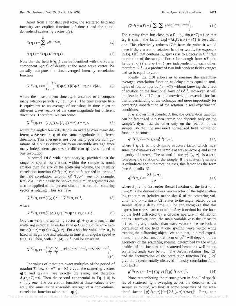
Figure 2 shows a plot of 11@gr(1)(q,t)#2 at the main

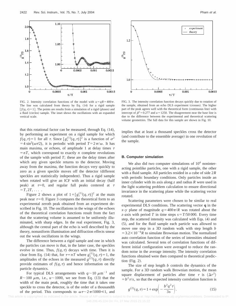
peak neart50. Figure 3 compares the theoretical form to anexperimental zeroth peak obtained from an experiment de-scribed in Fig. 10. The oscillations in the wings of the echoesof the theoretical correlation functions result from the factthat the scattering volume is assumed to be uniformly illu-minated, with sharp edges. In the real experiment, Fig. 3,although the central part of the echo is well described by thetheory, nonuniform illumination and diffraction effects smearout the weak oscillations in the wings.

The difference between a rigid sample and one in whichthe particles can move is that, in the latter case, the specklesevolve in time. Thus,f (q,t) decays with time. Then it isclear from Eq.~14! that, fort5nT wheregr

(1)(q,t)51, theamplitudes of the echoes in the measuredg(2)(q,t) directlyprovide estimates off (q,t) and hence information on theparticle dynamics.

For typical DLS arrangements withq;10 mm21 andR;100 mm, i.e., u;1000, we see from Eq.~13! that thewidth of the main peak, roughly the time that it takes onespeckle to cross the detector, is of the order of a thousandthof the period. This corresponds tovt;2p/1000!1, and

implies that at least a thousand speckles cross the detector~and contribute to the ensemble average! in one revolution ofthe sample.

B. Computer simulation

We also did two computer simulations of 104 noninter-acting pointlike particles, one with a rigid sample, the otherwith a fluid sample. All particles resided in a cube of side 2Rwith periodic boundary conditions. Only particles inside aninner cylinder with its axis alongz and radiusR were used inthe light scattering problem calculation to ensure directionalinvariance in the scattering plane while the scattering vectorrotated.

Scattering parameters were chosen to be similar to realexperimental DLS conditions. The scattering vectorq in thex-y plane of magnitudeq5400p/R was rotated about thez-axis with periodT in time stepss5T/50 000. Every timestep, the scattered intensity was calculated with Eqs.~4! and~5!, and for the fluid sample each particle was allowed tomove one step in a 3D random walk with step lengthb53.231026R to simulate Brownian motion. The normalizedauto correlation function of the series of intensities obtainedwas calculated. Several tens of correlation functions of dif-ferent initial configuration were averaged to reduce the ran-dom noise in the average intensity. The intensity correlationfunctions obtained were then compared to theoretical predic-tion ~Fig. 2!.

The size of step lengthb controls the dynamics of thesample. For a 3D random walk Brownian motion, the meansquare displacement of particles after timet is ^Dr 2&5b2t/s, so that the expected intensity correlation function is

g(2)~q,t!511expS 2b2q2t

3s D . ~15!

FIG. 2. Intensity correlation functions of the model withu5qR5400p.The line was calculated from theory by Eq.~14! for a rigid sample@ f (q,t)51#. The points are results from a simulation of a rigid~pluses! anda fluid ~circles! sample. The inset shows the oscillations with an expandedvertical scale.

FIG. 3. The intensity correlation function decays quickly due to rotation ofthe sample, obtained from an echo DLS experiment~crosses!. The higherpart of the peak agrees well with the theoretical form~continuous line! withintercept ofb250.277 andu51250. The disagreement near the base line isdue to the difference between the experimental and theoretical scatteringvolume geometries. The full data for this sample are shown in Fig. 10.

2422 Rev. Sci. Instrum., Vol. 75, No. 7, July 2004 Pham et al.

This article is copyrighted as indicated in the article. Reuse of AIP content is subject to the terms at: http://scitationnew.aip.org/termsconditions. Downloaded to IP:

148.206.45.224 On: Fri, 27 Mar 2015 21:15:22

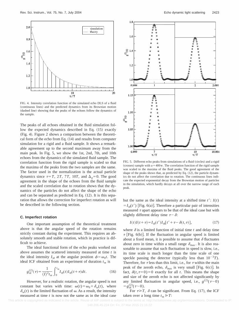
The peaks of all echoes obtained in the fluid simulation fol-low the expected dynamics described in Eq.~15! exactly~Fig. 4!. Figure 2 shows a comparison between the theoreti-cal form of the echo from Eq.~14! and results from computersimulation for a rigid and a fluid sample. It shows a remark-able agreement up to the second maximum away from themain peak. In Fig. 5, we show the 1st, 2nd, 7th, and 10thechoes from the dynamics of the simulated fluid sample. Thecorrelation function from the rigid sample is scaled so thatthe maxima of the peaks from the two samples are the same.The factor used in the normalization is the actual particledynamics sincet5T, 2T, 7T, 10T, andDq50. The goodagreement in the shape of the echoes from the fluid sampleand the scaled correlation due to rotation shows that the dy-namics of the particles do not affect the shape of the echoand can be separated as predicted in Eq.~12!. It is this sepa-ration that allows the correction for imperfect rotation as willbe described in the following section.

C. Imperfect rotation

One important assumption of the theoretical treatmentabove is that the angular speed of the rotation remainsstrictly constant during the experiment. This requires an ab-solutely smooth and stable rotation, which in practice is dif-ficult to achieve.

The ideal functional form of the echo peaks worked outabove assumes the scattered intensity measured at timet isthe ideal intensityI id at the angular positionf5v0t. Theideal ICF obtained from an experiment of durationtm is

gid(2)~t!5

1

^I &2tmE

0

tmI id~ t !I id~ t1t!dt. ~16!

However, for a realistic rotation, the angular speed is notconstant but varies with time:v(t)5v01dv(t), wheredv(t) is the limited fluctuation ofv. As a result, the intensitymeasured at timet is now not the same as in the ideal case

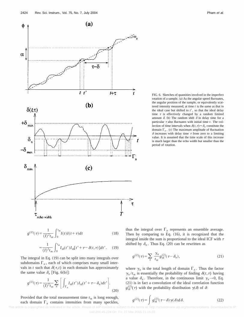
but the same as the ideal intensity at a shifted timet8: I (t)5I id(t8) @Fig. 6~a!#. Therefore a particular pair of intensitiesmeasuredt apart appears to be that of the ideal case but withslightly different delay timet2d:

I ~ t !I ~ t1t!5I id~ t8!I id@ t81t2d~ t,t!#, ~17!

whered is a limited function of initial timet and delay timet @Fig. 6~b!#. If the fluctuation in angular speed is limitedabout a fixed mean, it is possible to assume thatd fluctuatesabout zero in time within a small rangedmax. It is also rea-sonable to assume that such fluctuation in speed is slow, i.e.,its time scale is much longer than the time scale of onespeckle passing the detector~typically less than 1023T).Therefore, fort less than this limit, i.e., fort within the mainpeak of the zeroth echo,dmax is very small@Fig. 6~c!#. Infact, d(t,t50)50 exactly for all t. This means the shapeand size of the zeroth echo is not affected significantly byany limited fluctuation in angular speed, i.e.,g(2)(t;0)5gid

(2)(t;0).For t>T, d can be significant. From Eq.~17!, the ICF

taken over a long timetm @T:

FIG. 4. Intensity correlation function of the simulated echo DLS of a fluid~continuous lines! and the predicted dynamics from its Brownian motion~dashed line! showing that the peaks of the echoes follow the dynamics ofthe sample.

FIG. 5. Different echo peaks from simulations of a fluid~circles! and a rigid~crosses! sample withu5400p. The correlation function of the rigid samplewas scaled to the maxima of the fluid peaks. The good agreement of theshape of the peaks shows that, as predicted by Eq.~12!, the particle dynam-ics do not affect the correlation due to rotation. The continuous lines indi-cate the expected exponential decay from the Brownian motion of particlesin the simulation, which hardly decays at all over the narrow range of eachpeak.

2423Rev. Sci. Instrum., Vol. 75, No. 7, July 2004 Echo dynamic light scattering

This article is copyrighted as indicated in the article. Reuse of AIP content is subject to the terms at: http://scitationnew.aip.org/termsconditions. Downloaded to IP:

148.206.45.224 On: Fri, 27 Mar 2015 21:15:22

g(2)~t!51

^I &2tmE

0

tmI ~ t !I ~ t1t!dt ~18!

51

^I &2tmE

0

tmI id~ t8!I id@ t81t2d~ t,t!#dt8. ~19!

The integral in Eq.~19! can be split into many integrals oversubdomainsGn , each of which comprises many small inter-vals in t such thatd(t,t) in each domain has approximatelythe same valuedn @Fig. 6~b!#:

g(2)~t!51

^I &2tm(

nF E

Gn

I id~ t8!I id~ t81t2dn!dt8G .~20!

Provided that the total measurement timetm is long enough,each domainGn contains intensities from many speckles,

thus the integral overGn represents an ensemble average.Then by comparing to Eq.~16!, it is recognized that theintegral inside the sum is proportional to the ideal ICF withtshifted bydn . Thus Eq.~20! can be rewritten as

g(2)~t!5(n

gn

tmgid

(2)~t2dn!, ~21!

wheregn is the total length of domainGn . Thus the factorgn /tm is essentially the probability of findingd(t,t) havinga valuedn . Therefore, in the continuous limitgn→0, Eq.~21! is in fact a convolution of the ideal correlation functiongid

(2)(t) with the probability distributiong~d! of d:

g(2)~t!5E gid(2)~t2d!g~d!dd. ~22!

FIG. 6. Sketches of quantities involved in the imperfectrotation of a sample.~a! As the angular speed fluctuates,the angular position of the sample, or equivalently scat-tered intensity measured, at timet is the same as that inthe ideal case but shifted tot8, so that the ideal delaytime t is effectively changed by a random limitedamountd. ~b! The random shiftd in delay time for aparticulart also fluctuates with initial timet. The col-lection of time intervals whend(t,t)'dn constitute thedomainGn . ~c! The maximum amplitude of fluctuationd increases with delay timet from zero to a limitingvalue. It is assumed that the time scale of this increaseis much larger than the echo width but smaller than theperiod of rotation.

2424 Rev. Sci. Instrum., Vol. 75, No. 7, July 2004 Pham et al.

This article is copyrighted as indicated in the article. Reuse of AIP content is subject to the terms at: http://scitationnew.aip.org/termsconditions. Downloaded to IP:

148.206.45.224 On: Fri, 27 Mar 2015 21:15:22

The effect of this ‘‘smearing’’ of the correlation functionmeans that the apparent maximum of the main peak willdrop and the width will increase. However, it can be shownthat the area underg(2)(t) is the same as that undergid

(2)(t).Let us define thearea under the echo Aas the area betweenthe echo peak and the baselineg(2)(t)51 in the vicinity ofthe echo peak

A5EV

@g(2)~t!21#dt ~23!

52V1EV

g(2)~t!dt, ~24!

whereV is the integration interval around the echo peak andis large enough that the value of@gid

(2)(t)21# is zero at thelimits even if it is shifted by6dmax. Rewriting g(2)(t) interms of the convolution of the ideal ICF@Eq. ~22!#, oneobtains a double integral

A52V1EV

dtE2dmax

1dmaxdd gid

(2)~t2d!g~d!. ~25!

Becaused is constant fort within the rangeV of one echo,a change of variablev5t2d ~wheredv5dt! gives

A52V1EV8

gid(2)~v !dvE

2dmax

1dmaxg~d!dd. ~26!

Sincegid(2)(t) approaches a constant of 1 fort at the limits of

V, the new limitsV8 do not affect the first integral, thus itcan be separated from the second. The second integral isunity sinceg~d! is a normalized probability distribution func-tion. Thus the area under the real echo peakA is the same asthat under the ideal echo, independent of any smearing ef-fects

A52V1EV

gid(2)~v !dv5Aid . ~27!

It has been shown in Sec. II A that the measured corre-lation function can be factorized into the particle dynamicsand the rotation correlation, so that Eqs.~2! and ~12! give

gid(2)~t!215b2@ f ~q,t!#2@gr

(1)~t!#2, ~28!

whereb2 is the usual intercept in the Siegert relation.Combining Eqs.~23!, ~27!, and~28!, the area under the

nth echo measures the dynamics free of interference from thesmearing effect of imperfect rotation

An5An, id5Et;tn

b2@ f ~q,t!#2@gr(1)~t!#2. ~29!

If the dynamics is slow compared to the rotation, the particledynamicsf (q,t) is virtually unchanged over the very narrowtime range of one echo width~see the solid line in Fig. 5!.Thus f (q,t) is constant:f (q,t)5 f (q,tn), wheretn is theposition of thenth echo maximum, and can be taken out ofthe integral

~30!

where the remaining integral is in fact the area under thezeroth echo. Therefore the real dynamics simply scale thearea under an echo by a factor of@ f (q,tn)#2 relative to thezeroth echo. It should be noted that for samples wheref (q,t) decays significantly in the short time regime corre-sponding to about half an echo width (t,1023T), the inte-gral in Eq.~30! is in fact larger than the area under the zerothecho. However, the scaling of areas of all other echoes stillholds. In practice, sincef (q,t) obtained in echo DLS needsto be rescaled by an arbitrary factor as explained at the end

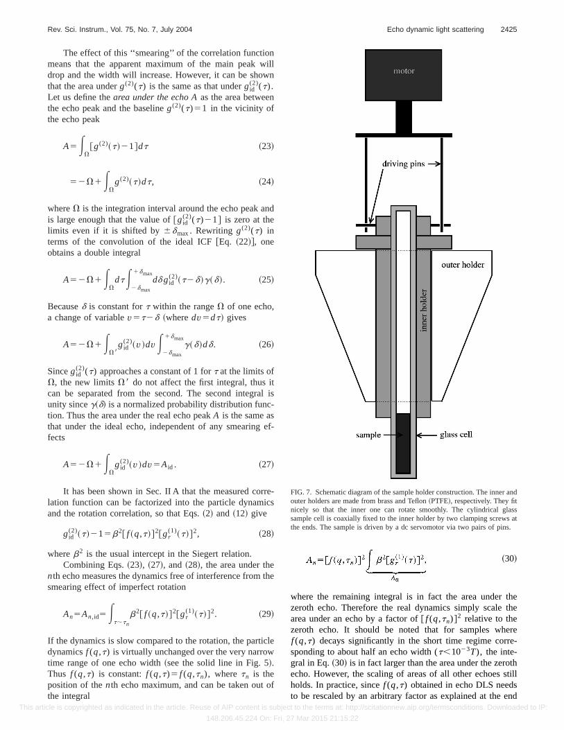
FIG. 7. Schematic diagram of the sample holder construction. The inner andouter holders are made from brass and Teflon~PTFE!, respectively. They fitnicely so that the inner one can rotate smoothly. The cylindrical glasssample cell is coaxially fixed to the inner holder by two clamping screws atthe ends. The sample is driven by a dc servomotor via two pairs of pins.

2425Rev. Sci. Instrum., Vol. 75, No. 7, July 2004 Echo dynamic light scattering

This article is copyrighted as indicated in the article. Reuse of AIP content is subject to the terms at: http://scitationnew.aip.org/termsconditions. Downloaded to IP:

148.206.45.224 On: Fri, 27 Mar 2015 21:15:22

of Sec. IV, the exact value of the area under the zeroth echois not important in measuring the shape off (q,t).

III. IMPLEMENTATION AND DATA ANALYSIS

Below we describe the implementation of experimentalarrangements and data analysis for this technique. The DLSsetup employed here is two-color DLS20 to extract singlescattering information from turbid samples. However, if con-ventional DLS were used, all following details still hold witha replacement of the two-color intensities by the single colorintensity.

A. Instrument setup and data acquisition

The sample was put into a cylindrical glass cell withouter diameter'7 mm which was secured into a sampleholder that rotated with little friction about the optical axis ofthe setup~Fig. 7!. The sample holder was driven by a dcservomotor via two perpendicular pairs of pins, one on theholder and the other connected to the motor. This ‘‘pin-driving’’ mechanism decoupled any wobbling between themotor and the sample, making it unnecessary to align themotor axis exactly to the optical axis of the DLS setup. Theconstruction of the sample holder alone ensured the samplewas at the center of the setup, and needed to be checked onlyonce.

The intensity I (t) in the far field was measured bycounting the number of photons that arrived at the detector inthe time interval@ t,t1s#, where the length of this intervalswas called thesample time. Therefore the intensity can onlybe realized as discrete numbers of photon counts in discreteunits of sample times, which is typically a few tens ofmicroseconds or less. The cross correlation function of theblue intensityI B(t) and the green intensityI G(t) was con-structed as

g(2)~k!5M( j 51

M I B~ j !I G~ j 1k!

~( j 51M I B~ j !!~( j 51

M I G~ j 1k!!, ~31!

where g(2)(k) is the correlation function at delay timet5ks and I ( j ) represents the photon counts at timet5 js.This formulation of the correlation function where the de-nominator is the product of the averages of direct intensityI ( j ) and delayed intensityI ( j 1k) is calledsymmetric nor-malization. This method of normalization improves the accu-racy of the result if the input intensity varies slowly.26

Since this scheme requires correlating the intensity atone speckle with that at exactly the same place after somedelay timet, it is necessary that a linear sampling scheme isused. This means the sample times has to be constant for alldelay timest. In order to calculate the correlation functionfor a large delay timet of say 1000 s, a very large number ofsamples (t/s'108) have to be stored in a buffer. The con-straint of storing a large number of samples makes softwarecorrelation more effective and inexpensive than using a hard-ware correlator, especially with increasing processing speedof modern personal computers~PC!.

Photon counts were acquired by a counter card~PCI-6602 purchased from National Instrument, USA! on an ex-tension slot of a PC with a simple software program. Thecard was configured to count the number of detected photonpulses during every sample times. The speed limitation ofthe interface between the card and the computer memorymeans the sample time has to be larger than 6ms. The countsfrom each detector were saved as series of integers in com-puter files. The correlation function was then calculatedseparately and simultaneously on the raw data files by an-other program according to Eq.~31!.

B. Modified multitau scheme

For almost all cases, a very large range of dynamicalinformation is of interest. Therefore one will usually need toknow the correlation function at logarithmically spaced delaytimes. As a result, a very large amount of information ‘‘be-tween the points’’ at larget is not used. In order to make useof this ‘‘lost’’ information, Schatzel introduced the multitauscheme,27 in which the sample time used to calculate a cor-relation channel is proportional to the delay time of thatchannel. However, in echo DLS the requirement of correlat-ing intensity at one speckle to that at the same speckle a longtime afterwards is absolutely crucial. Thus a simple multitauscheme as in Ref. 27 is not possible as it averages intensitiesof neighboring speckles in the process.

FIG. 8. Modified multitau scheme for the echo DLS method. Pairs of countsfrom the same angular position are averaged to give a new count sample.These make up a sample stream with effectively double the sample time.The streams are then used to calculate the correlation function in the sameway for larger delay times. This procedure is repeated several times.

TABLE I. A typical choice for the effective sample time and the correlationdelay time. There are 16 echoes in the first partition, then 8 every subse-quent octave. The sample time is doubled every step, and thus the totalnumber of samples is halved. The total time for calculating the correlationfunction is therefore reduced.

Effectivesampletime

Sampletemporalcoverage Echoes Range int

Original data s s 0–16 1–16TFirst average 2s T 9–16 18–32TSecond average 4s 3T 9–16 36–64TThird average 8s 7T 9–16 72–128T. . . . . . . . . . . . . . .nth average 2ns (2n21)T 9–16 ~9–16! 32nT

2426 Rev. Sci. Instrum., Vol. 75, No. 7, July 2004 Pham et al.

This article is copyrighted as indicated in the article. Reuse of AIP content is subject to the terms at: http://scitationnew.aip.org/termsconditions. Downloaded to IP:

148.206.45.224 On: Fri, 27 Mar 2015 21:15:22

We introduced a modified multitau scheme where corre-lation between intensities at exactly the same speckle wasmaintained while the sample times was effectively increasedfor increasing delay time. The main feature of this modifiedscheme was that the effective sample time was increased byaveraging intensities at exactly the same speckle at neighbor-ing revolution ~Fig. 8!. Intensities from the same angularposition at two consecutive periods were averaged to giveone new sample. Thus the effective sample time for eachnew sample was now twice the old one. The new averagedvalues were then put into new streams which were correlatedin the same way for longer delay time. In order to ensure thatintensities at the same speckle were added, a precise mea-surement of the period was required. This value was readilyavailable by computing at least one echo from the originalintensity without using multitau. The position of this echoallows the period to be calculated with relative uncertainty ofabout 1026.

Although the sample time was doubled, the actual twosamples that were averaged were separated by one period intime. Therefore the delay time of the correlation channelcalculated with the averaged sample time must be consider-ably larger than one period to reduce distortion due to aver-aging. In this scheme, we used the original data stream tocalculateg(2)(t) up to the 16th echo. Then the sample time

was doubled and the new stream was used forg(2)(t) fromthe 9th to 16th echo of the new sample time, which corre-sponds to echoes 18 to 32 of the original sample time. Thiswas repeated as many times as necessary to achieve the long-est delay time. The procedure is summarized in Table I. Thisselection of sample time and delay time ensured that thedelay time was at least nine times larger than the separationbetween averaged samples, which introduced a triangulardistortion of no more than 1023.27

The use of this scheme reduces the total number ofsamplesM that have to be correlated for larget, thus reducescalculation time significantly. In a typical experiment (s540ms, 100 delay channels in each echo, 70 echoes in totalcovering the ranget512104 s with a maximum of 20 ech-oes per decade! with measurement timetm51.53104 s, cal-culation of the ICF on a 2 GHz Pentium IV computer takesapproximately 5 h (1.83104 s) and requires 715 MB of harddisk space for one intensity stream. As data acquisition andthe ICF calculation can be performed independently and inparallel, echo DLS can be operated almost in real time witha fast computer. However computing speed is not a strictrequirement as raw data can be processed off-line or simul-taneously in many computers.

C. Smearing correction

Imperfect sample rotation and its smearing effect wereobserved in almost all measurements. The effects introducesignificant noise and even systematic error to the maximumvalues of the echoes~Fig. 9!. It was shown in Sec. II C thatin such cases, it is essential to use the area under the echopeak to measure the intrinsic dynamics of the sample. Thenormalization by area is done as follows. First, the area un-der each echo and above the baseline,A(tn), including thezeroth echo, is calculated

A~tn!5Et;tn

@g(2)~t!21#dt, ~32!

whereg(2)(t) is the measured ICF. The integral limits willbe discussed in Sec. III D.

Knowing the area under the echo is conserved undersmearing but scaled by the dynamics@Eq. ~30!#, thesmearing-corrected correlation functiongs

(2)(tn)[11b2@ f (q,tn)#2 at echon was then constructed as

gs(2)~tn!5

A~tn!

A~t0!@g(2)~0!21#11, ~33!

whereA(tn) andA(t0) are the areas under thenth and thezeroth echoes, respectively;g(2)(0) is the maximum value ofthe zeroth echo,g(2)(t50).

It might be expected that the application of the modifiedmultitau scheme to improve statistical accuracy would tendto ‘‘average out’’ the effect of smearing. Thus the additionalsmearing correction might not have the same effect as rigor-ously proved in Sec. II C. However, in practice it seemed thateven though the modified multitau scheme reduced the ran-dom fluctuation due to smearing from one echo to the next, itdid not eliminate the accumulated smearing effect@the rise inrelative FWHM att'53103 s in Fig. 9~a!#. Yet the smear-

FIG. 9. Correlation function from a rigid sample~made by centrifuging acolloidal suspension to give a solid amorphous sediment!, calculated withthe modified multitau scheme.~a! The vertical lines are echoes with largefluctuations at lowt, due to smearing, and more systematic changes at larget. The squares correspond to full widths at half maximum~FWHM! of theechoes, measured relative to the FWHM of the zeroth echo, scales on right.~b! Smearing corrected correlation functions using different area integrationschemes. There are offsets between the schemes but data within eachscheme are consistent and more accurate than without correction.

2427Rev. Sci. Instrum., Vol. 75, No. 7, July 2004 Echo dynamic light scattering

This article is copyrighted as indicated in the article. Reuse of AIP content is subject to the terms at: http://scitationnew.aip.org/termsconditions. Downloaded to IP:

148.206.45.224 On: Fri, 27 Mar 2015 21:15:22

ing correction seemed to eliminate that almost entirely@Fig.9~b!#. Many experiments carried out on rigid samplesshowed that the smearing correction worked well with themodified multitau scheme.

The above smearing correction however does not verifythe assumption that the fluctuation in rotating angular speedis limited and the average speed is stable over the wholeexperiment. To verify this assumption and monitor the extentof the smearing effect, one can use another feature of theecho: the full widths at half maximum~FWHMs! of thepeaks above the baseline. Since the FWHM is not dependenton the area under each echo, i.e., independent of the intrinsicdynamics of the sample, it is a good candidate as a measureof the ‘‘quality’’ of the rotation. The relative FWHM com-pared to that of the zeroth echo is a measure of the extent ofsmearing on the shape of the obtained echo@Fig. 9~a!#. For aperfectly constant speed of rotation, the values of all FWHMof all echoes should be the same as that of the zeroth echo,therefore all relative FWHMs should be equal to one. If therotation is not completely smooth, smearing will occur andthe relative FWHMs will not be constant and will be greaterthan one. If the rotation speed is not stable, e.g., the averagespeed changes due to large friction, the relative FWHM willdiverge at larget. Sometimes, particularly in measurementsmade immediately after the outer sample holder~Fig. 7! hadbeen replaced, such divergence of the FWHM was observed.Thus, by monitoring the FWHM as a function oft, one canevaluate the quality of the rotation and discard data forwhich velocity drift is excessive.@Note that, although theFWHMs in Fig. 9~a! show significant variation at larget,they remain bounded and the smearing correction, Fig. 9~b!,works well.#

D. Area limits

There are several ways to choose the integration limits inEq. ~32!. Theoretically, the correlation functiong(2)(t) isnever less than and approaches the baseline value of 1 awayfrom the main peak. However, in almost all measurements,g(2)(t) fluctuates about 1 even very far from the echo peak.This fluctuation is due to random noise in the average inten-sity used for normalization from the limited number of inde-pendent speckles observed. Our typical experimental setupobserved aboutp5T/(echo width);3000 speckles, whichgives a random error ofA1/p'2%. This uncertainty alsoapplies to the intercept of the ICF. This fluctuation in thebaseline is unavoidable and too complicated to correct for inthe data analysis. Instead we tried different empirical limitsto calculate the area and typical results for a rigid sample arepresented in Fig. 9~b!. The measured correlation function isthe result of an ideal echo superimposing on a fluctuatingbackground around 1. Furthermore, the relative position ofthe real echo changes with respect to minima and maxima ofthe background, and it seems that it is this relative positionthat complicates the choice of the most appropriate limits.The simplest choice is the ‘‘baseline’’ limit. The limits ofintegration are chosen to be the last point above 1 whenmoving away from the peak of the echo. This works rela-tively well in some cases. However, in case where the echo

does not reach 1 in a rather large range oft, several back-ground fluctuations are included in the area calculation. Re-sults in these cases are not very smooth.

Another simple choice is the ‘‘minimum’’ limit, wherethe first local minima ing(2)(t) either side of the peak areused as limits. This method seems to work well with quicklydecaying ICF from ergodic samples, where the backgroundfluctuation is very small due to a large number of indepen-dent speckles observed. In most of the other cases it does notgive very good results, usually with a few points having veryhigh or very low values@squares in Fig. 9~b!#.

The last choice is the ‘‘fixed-width’’ limit where therange of integration is fixed to the same value either side ofthe peak and the same for all echoes, including the zerothecho. This method seems to work relatively well for mostcases. However, the difficulty is to make the right choice ofthe integration width. Ideally, one would like to calculate thearea with an infinite width to average out all fluctuations inthe background. However, even if that approach were prac-tical, the area calculated would not converge but fluctuateabout a mean value. It is this mean value that we need for thearea. It was found that a value for the width equal to a mul-tiple ~no less than the maximum value of the relativeFWHM! of the zeroth echo widthw0 produced rather goodresults, withw0 defined by the first minimum ing(2)(t) inthe zeroth echo. Even the choice of integration limits madeseemed somewhat arbitrary to make the end result ofgs

(2)(t)a smooth function, the correction eliminated spurious fluc-tuations in the original data due to imperfect rotation, yet didnot introduce any other except from small random noise.

IV. DISCUSSION

A comparison of the dynamic structure factorsf (q,t)obtained using echo DLS and by brute-force averaging of

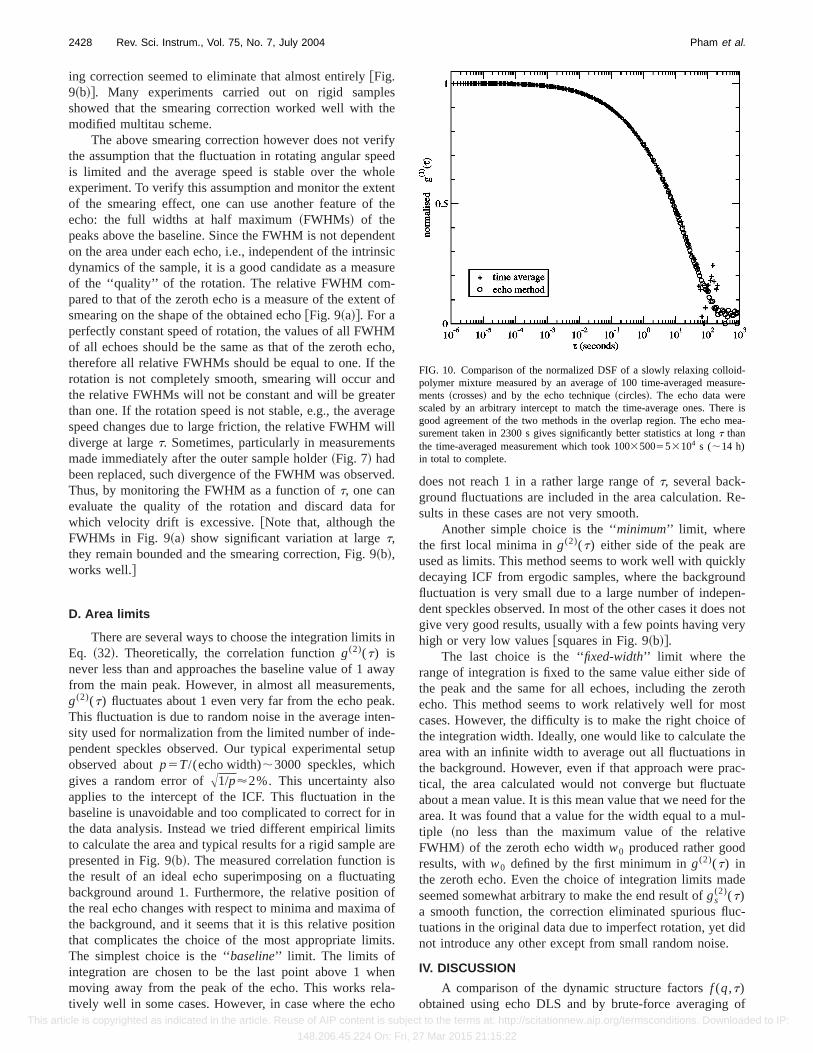
FIG. 10. Comparison of the normalized DSF of a slowly relaxing colloid-polymer mixture measured by an average of 100 time-averaged measure-ments ~crosses! and by the echo technique~circles!. The echo data werescaled by an arbitrary intercept to match the time-average ones. There isgood agreement of the two methods in the overlap region. The echo mea-surement taken in 2300 s gives significantly better statistics at longt thanthe time-averaged measurement which took 1003500553104 s (;14 h)in total to complete.

2428 Rev. Sci. Instrum., Vol. 75, No. 7, July 2004 Pham et al.

This article is copyrighted as indicated in the article. Reuse of AIP content is subject to the terms at: http://scitationnew.aip.org/termsconditions. Downloaded to IP:

148.206.45.224 On: Fri, 27 Mar 2015 21:15:22

100 conventional time-averaged correlation functions of ametastable ergodic colloid-polymer sample atq514.51mm21 is presented in Fig. 10. A more detailed de-scription of this sample can be found in Refs. 7 and 8. In theoverlap region, delay timet.1s, excellent agreement isfound between the results of the two measurements. Notethat, because echo DLS averages over several thousandspeckles, the echo data are of much better quality at largetdespite a 20-fold shorter measurement time. This goodagreement of the two techniques, along with the agreementbetween experiment and theory for a rigid sample~Fig. 9!,provides convincing evidence that the echo DLS method cangive very good quality data in a short measurement time.

Ideally, the measurement timetm required to obtain dy-namical data at the maximum delay timetmax is just tmax

plus one period for ensemble averaging at the longest delaytime: tm5tmax1T. Even with imperfection in rotation, themeasurement time is required to extend for only a few hun-dred periods beyondtmax to average over all fluctuations inangular speed, so thattm is still of the order oftmax. Withtoday’s computer speed and hard drive capacity, computingthe correlation function with the modified multitau schemetook about the same timetm as for acquiring the data. Thusecho DLS can be operated almost in real time. There is, inprinciple, no upper limit fortmax other than the patience ofthe experimenter. One can easily obtain dynamical informa-tion up to a delay time of 104 s in about 1.53104 s ~4 h! ofmeasurement time.

By contrast, acquiring a time-averaged correlation func-tion at the sametmax requires a measurement time of manytimes tmax. For nonergodic samples, several hundreds oftime-averaged ICF’s are needed to obtain proper ensemble-averaged dynamics. This pushes the total measurement timeto the order of;1000tmax. Therefore to measure dynamicsof a non-ergodic sample up tot51000 s, normal brute-forceensemble averaging methods requires;106 s ~12 days! ofmeasurement time, whereas echo DLS only takes less thanan hour, yet produces much better data as it samples thou-sands of independent speckles.

Compared to other methods of measuring nonergodicdynamics, echo DLS has certain advantages. First, it doesnot require high spatial coherence over detector aperture asin the method of Pusey and van Megen.14 In fact, intensitycorrelation functions with any intercept, i.e., any level ofcoherence, can be measured with echo DLS. Therefore thetechnique is suitable for use in cross-correlation schemes liketwo-color20 or three-dimensional21 DLS where, because ofmultiple scattering, the intercept depends on sample turbidityand is usually significantly lower than one.

Second, compared to ‘‘multispeckle’’ experiments,16–18

where charge coupled device cameras are used as array de-tectors, echo DLS can average the dynamics over a muchlarger number of speckles, typically several thousands~theratio of the rotation period to the echo width!, without com-promising the resolution of scattering angle. Thus randomnoise in the data due to the limited number of independentspeckles sampled is lower with echo DLS. This noise is par-ticularly pronounced in highly nonergodic samples, i.e.,

samples whose measured dynamics are highly frozen andhave a high value off (q,`).

Finally, we compare echo DLS with the interleaved sam-pling method19 ~also, Ref. 2!. Both methods use essentiallythe same hardware: The sample is rotated in otherwise stan-dard light scattering equipment. In echo DLS, the photo-counts from the detector are regarded as a single stream ofdata which is autocorrelated~or, in the case of two-colorDLS or 3D DLS, two data streams which are cross-correlated!. Dynamic information about the sample is de-rived from the amplitudes and areas of echoes in the corre-lation function. In interleaved sampling, the technique isessentially regarded as performing many different experi-ments. The software effectively comprises thousands ofseparate correlators, one for each speckle in the sequencethat crosses the detector as the sample is rotated. Thus eachcorrelator is associated with a specific position of the sample,and consecutive intensity measurements for this correlatorare taken after every full rotation of the sample. At the end ofthe measurement, each correlator has measured the time-averaged behavior of a particular speckle. The desiredensemble-averaged correlation function, single points att5nT, is then obtained by summing the thousands of time-averaged measurements. The advantage of echo DLS is thatit calculates the correlation function over a range of delaytimes aroundt5nT, allowing, as described above, the areasof the echoes to be used to correct the data for the effect ofimperfect rotation. Furthermore, it is not necessary to syn-chronize the sample’s rotation with the clock in the computerused to calculate the correlation function. This allows one touse a continuous servomotor, as opposed to the stepper mo-tor used in interleaved sampling, to produce a smooth rota-tion.

The main drawback of echo DLS, shared by the inter-leaved sampling method, is the lack of data fort,T, whichis typically about one second. Any much faster rotation canproduce, apart from mechanical difficulties, instability of ro-tational speed and possible unwanted disturbance to thesample. Therefore some other methods such as brute-forceensemble averaging8 or slow rotation15 should be used toobtain short time data up tot;10 s. These data joined withecho DLS allow one to measure dynamics of nonergodicsamples over a very large dynamic range, typically from1026 to 104 s.

The interceptg(2)(0) obtained with echo DLS was usu-ally less than that obtained in brute-force ensemble averag-ing. This appears to be caused by slight ‘‘wobbling’’ of thesample about the vertical axis during rotation. Thus, even fora rigid sample, the speckles do not return exactly to the de-tector aftern rotations, but may be displaced slightly up ordown. This effect was instrument-related and different in dif-ferent samples and at different scattering angles, and thuswas very difficult to determine or calibrate. It can be argued,however, that, because the motion occurs in planes perpen-dicular to the plane of rotation, all the echoes are affected inthe same way which can be described by a reduction in thefactor b2. Therefore in order to join echo data to those ob-tained by ensemble averaging at shorter delay time, the in-tercept was scaled by an arbitrary factor~in the range 1–2! to

2429Rev. Sci. Instrum., Vol. 75, No. 7, July 2004 Echo dynamic light scattering

This article is copyrighted as indicated in the article. Reuse of AIP content is subject to the terms at: http://scitationnew.aip.org/termsconditions. Downloaded to IP:

148.206.45.224 On: Fri, 27 Mar 2015 21:15:22

match with data obtained by other techniques in the region ofoverlap.

ACKNOWLEDGMENTS

It is a pleasure to thank Phil Francis for valuable adviceon building the sample holder: The original design of theholder construction was from the Colloids Laboratory atRMIT University, Australia. We also thank G. Petekidis andD. A. Weitz for fruitful discussions. KNP holds a U.K. ORSaward. Financial support for this project came from EPSRCgrants GR/M92560 and GR/S10377/01, and Unilever Re-search U.K.

APPENDIX A: SEPARATION OF DYNAMICS ANDROTATION

First it is worth stating a key theorem that will be used inthe following analysis. If two discret variablesx and y areindependent, then the product of the statistically significantaverage of their product is the same as the product of theiraverages:xy&5^x&^y&. More explicitly

(i 51

N

xiyi51

N (j 51

N

(k51

N

xjyk . ~A1!

The time-averaged unnormalized field correlation functionfrom Eq. ~10! is

~A2!

Let us consider the quantity inside the average at a fixedtime t, thus also at fixed vectorsq andDq . Upon changingthe indexk, we will show that the phase factorsP and Qchange independently of each other. Strictly speaking,P de-pends on the exact value ofr k . However, one may noticethat the contribution of all particlesj far enough from par-ticle k, i.e., ur j2r ku@2p/q, to P does not depend on theexact position of particlek. The otherj particles that con-tribute to P are those in the vicinity of particlek, within aregion of size;2p/q aroundr k . If this size is much smallerthan the size of the scattering volumeR, an insignificantnumber ofPk’s depend onr k due to the dependence of thedistribution ofr j2r k on r k . Furthermore, if one assumes thatthe sample is isotropic and there is no external field on theparticles and no centrifugation, then the distribution of par-ticle positions$r j (t)% bear no relation to where particlek is.Thus P does not depend onr k(t1t), i.e., it is independentof Q.

Using the theorem stated earlier, one can write the sumover k as a double sum overk and l :

G(1)~q,t!

51

N K (l 51

N

(k51

N

(j 51

N

eiq[ r j (t)2rk(t1t)]e2 i Dqr l (t1t)L ~A3!

51

N K (k51

N

(j 51

N

eiq[ r j (t)2rk(t1t)](l 51

N

e2 i Dqr l (t1t)L . ~A4!

As t changes, both vectorsq andDq rotate by the sameangle. However, the resulting changes in the two sums in theabove equation are not correlated as they are measures ofdifferent quantities. The change in the first sum depends onthe distribution of displacement vectors of all particles in thescattering volume, whereas the change in the second sumdepends on the distribution of the position vectors of theparticles. With the assumption that the sample is homoge-neous and there is no external field, these two distributionsare independent of each other. Therefore we can split theaverage~over q! of the product to a product of averages

G(1)~q,t!51

N K (j 51

N

(k51

N

eiq[ r j (t)2rk(t1t)] L3K (

l 51

N

e2 i Dqr l (t1t)L . ~A5!

This shows the separation in the correlation function be-tween sample dynamics~the first factor—the unnormalizedcollective dynamic structure factor! and rotation of thesample ~the second factor!. Normalization by the factor( j (k^e

iq[ r j (t)2rk(t)]& gives rise to Eq.~12!, where the rotationfactor gr

(1) is given by

gr(1)~q,t!5

1

N (l 51

N

^e2 i Dqr l (t1t)&. ~A6!

APPENDIX B: THEORETICAL ECHO SHAPE

This Appendix solves Eq.~A6! for an analytical form ofthe rotation factiongr

(1) . We can rewrite the ensemble aver-age overDq in Eq. ~A6! in its time-average form

gr(1)~q,t!5

1

N (l 51

N1

tmE

0

tme2 i Dq(t,t)r l (t1t)dt, ~B1!

where the productDqr l can be expressed in scalar terms:Dqr l cos(vt) asDq rotates in time with angular speedv. Theintegrand is a periodic function of time—F@cos(vt)#, the in-tegral of which over a long enough durationtm much greaterthan the rotation periodT will give the same result as ifintegrated over the distribution of the phasef5vt:

1

tmE

0

tm@T

F@cos~vt !#dt51

2p E0

2p

F@cos~f!#df. ~B2!

Assuming that the sample is homogeneous, the sum overl in Eq. ~B1! can be written as an integral over the distribu-tion of r inside the scattering volume

1

N (l 51

N

F@r #5E0

R 2pr

pR2 F@r #dr. ~B3!

2430 Rev. Sci. Instrum., Vol. 75, No. 7, July 2004 Pham et al.

This article is copyrighted as indicated in the article. Reuse of AIP content is subject to the terms at: http://scitationnew.aip.org/termsconditions. Downloaded to IP:

148.206.45.224 On: Fri, 27 Mar 2015 21:15:22

Using results in Eqs.~B2! and~B3!, the rotation factor inEq. ~B1! becomes

gr(1)~q,t!5

1

pR2 E0

R

drE0

2p

df re2 iDqr ~B4!

52J1~DqR!

DqR, ~B5!

where Dq52q sin(vt/2) ~Fig. 1! and J1(x) is a first-orderBessel function of the first kind. We make a change of vari-able to more intuitive quantities. We putu5qR, ands52 sin~vt/2!. Then DqR52qRsin(vt/2)5us. The rota-tional correlation then has the form of Eq.~13!.

1L. Cipelletti and L. Ramos, Curr. Opin. Colloid Interface Sci.7, 228~2002!.

2W. van Megen, T. C. Mortensen, S. R. Williams, and J. Mu¨ller, Phys. Rev.E 58, 6073~1998!.

3J. Bergenholtz and M. Fuchs, J. Phys.: Condens. Matter11, 10171~1999!;12, 6575~2000!.

4K. Dawson, G. Foffi, M. Fuchs, W. Go¨tze, F. Sciortino, M. Sperl, P.Tartaglia, Th. Voigtmann, and E. Zaccarelli, Phys. Rev. E63, 011401~2000!.

5K. N. Pham, A. M. Puertas, J. Bergenholtz, S. U. Egelhaaf, A. Moussaı¨d,P. N. Pusey, A. B. Schofield, M. E. Cates, M. Fuchs, and W. C. K. Poon,Science296, 104 ~2002!.

6T. Eckert and E. Bartsch, Phys. Rev. Lett.89, 125701~2002!.7W. C. K. Poon, K. N. Pham, S. U. Egelhaaf, and P. N. Pusey, J. Phys.:Condens. Matter15, S269~2003!.

8K. N. Pham, S. U. Egelhaaf, P. N. Pusey, and W. C. K. Poon, Phys. Rev.E 69, 011503~2004!.

9L. Cipelletti, S. Manley, R. C. Ball, and D. A. Weitz, Phys. Rev. Lett.84,2275 ~2000!.

10L. Ramos and L. Cipelletti, Phys. Rev. Lett.87, 245503~2001!.11M. Bellour, A. Knaebel, J. L. Harden, F. Lequeux, and J.-P. Munch, Phys.

Rev. E67, 031405~2003!.12J. Torok, S. Krishnamurthy, J. Kerte´sz, and S. Roux, Phys. Rev. Lett.84,

3851 ~2000!.13J. Torok, S. Krishnamurthy, J. Kerte´sz, and S. Roux, Phys. Rev. E67,

026108~2003!.14P. N. Pusey and W. van Megen, Physica A157, 705 ~1989!; P. N. Pusey,

Macromol. Symp.79, 17 ~1993!.15J.-Z. Xue, D. J. Pine, S. T. Milner, X.-I. Wu, and P. M. Chaikin, Phys. Rev.

A 46, 6550~1992!.16A. P. Y. Wong and P. Wiltzius, Rev. Sci. Instrum.64, 2547~1993!.17L. Cipelletti and D. A. Weitz, Rev. Sci. Instrum.70, 3214~1999!.18S. Kirsch, V. Frenz, W. Schartl, E. Bartsch, and H. Sillescu, J. Chem.

Phys.104, 1758~1996!.19J. Muller and T. Palberg, Prog. Colloid Polym. Sci.100, 121 ~1996!.20P. N. Segre`, W. van Megen, P. N. Pusey, K. Scha¨tzel, and W. Peters, J.

Mod. Opt.42, 1929~1995!.21E. Overbeck, C. Sinn, T. Palberg, and K. Scha¨tzel, Colloids Surf., A122,

83 ~1997!.22P. Hebraud, F. Lequeux, and J. P. Munch, Phys. Rev. Lett.78, 4657

~1997!.23R. Hohler, S. Cohen-Addad, and H. Hoballah, Phys. Rev. Lett.79, 1154

~1997!.24G. Petekidis, A. Moussaı¨d, and P. N. Pusey, Phys. Rev. E66, 051402

~2002!.25P. N. Pusey, inPhoton Correlation Spectroscopy and Velocimetry, edited

by H. Z. Cummins and E. R. Pike~Plenum, New York, 1977!, pp. 45–141.26K. Schatzel, M. Drewel, and S. Stimac, J. Mod. Opt.35, 711 ~1988!.27K. Schatzel, Inst. Phys. Conf. Ser.77, 175 ~1985!.

2431Rev. Sci. Instrum., Vol. 75, No. 7, July 2004 Echo dynamic light scattering

This article is copyrighted as indicated in the article. Reuse of AIP content is subject to the terms at: http://scitationnew.aip.org/termsconditions. Downloaded to IP:

148.206.45.224 On: Fri, 27 Mar 2015 21:15:22