jontalle.web.engr.illinois.edu11_49.pdf · Contents 1 Introduction 13 1.1 Early history . . . . . ....
317
An Invitation to Mathematical Physics and Its History Jont B. Allen Copyright © 2016,17,18,19 Jont Allen University of Illinois at Urbana-Champaign Saturday 3 rd August, 2019 @ 11:49; Version 1.00.0
Transcript of jontalle.web.engr.illinois.edu11_49.pdf · Contents 1 Introduction 13 1.1 Early history . . . . . ....

An Invitation to Mathematical Physicsand Its History
Jont B. AllenCopyright © 2016,17,18,19 Jont Allen
University of Illinois at Urbana-Champaign
Saturday 3rd August, 2019 @ 11:49; Version 1.00.0

2

Contents
1 Introduction 131.1 Early history . . . . . . . . . . . . . . . . . . . . . . . . . . . . . . . . . . . . . . . . . 13
1.1.1 Three Streams from the Pythagorean theorem . . . . . . . . . . . . . . . . . . . 151.1.2 What is science? . . . . . . . . . . . . . . . . . . . . . . . . . . . . . . . . . . 161.1.3 What is mathematics? . . . . . . . . . . . . . . . . . . . . . . . . . . . . . . . 161.1.4 Early physics as mathematics . . . . . . . . . . . . . . . . . . . . . . . . . . . 18
1.2 Modern mathematics is born . . . . . . . . . . . . . . . . . . . . . . . . . . . . . . . . 181.2.1 Science meets mathematics . . . . . . . . . . . . . . . . . . . . . . . . . . . . . 181.2.2 The Three Pythagorean Streams . . . . . . . . . . . . . . . . . . . . . . . . . . 24
2 Stream 1: Number Systems 252.1 The taxonomy of numbers: P,N,Z,Q,F, I,R,C . . . . . . . . . . . . . . . . . . . . . 26
2.1.1 Numerical taxonomy: . . . . . . . . . . . . . . . . . . . . . . . . . . . . . . . . 292.1.2 Applications of integers . . . . . . . . . . . . . . . . . . . . . . . . . . . . . . 30
2.2 Exercises NS-1 . . . . . . . . . . . . . . . . . . . . . . . . . . . . . . . . . . . . . . . 342.3 The role of physics in mathematics . . . . . . . . . . . . . . . . . . . . . . . . . . . . . 37
2.3.1 The three streams in mathematics . . . . . . . . . . . . . . . . . . . . . . . . . 372.3.2 Stream 1: Prime number theorems . . . . . . . . . . . . . . . . . . . . . . . . 382.3.3 Stream 2: Fundamental theorem of algebra . . . . . . . . . . . . . . . . . . . . 392.3.4 Stream 3: Fundamental theorems of calculus . . . . . . . . . . . . . . . . . . . 392.3.5 Other key theorems in mathematics . . . . . . . . . . . . . . . . . . . . . . . . 39
2.4 Applications of Prime number . . . . . . . . . . . . . . . . . . . . . . . . . . . . . . . 402.4.1 The Euclidean algorithm (GCD) . . . . . . . . . . . . . . . . . . . . . . . . . . 42
2.5 Exercises NS-2 . . . . . . . . . . . . . . . . . . . . . . . . . . . . . . . . . . . . . . . 472.5.1 Continued fractions . . . . . . . . . . . . . . . . . . . . . . . . . . . . . . . . . 532.5.2 Pythagorean triplets (Euclid’s formula) . . . . . . . . . . . . . . . . . . . . . . 562.5.3 Pell’s equation . . . . . . . . . . . . . . . . . . . . . . . . . . . . . . . . . . . 572.5.4 Fibonacci sequence . . . . . . . . . . . . . . . . . . . . . . . . . . . . . . . . . 59
2.6 Exercises NS-3 . . . . . . . . . . . . . . . . . . . . . . . . . . . . . . . . . . . . . . . 62
3 Stream 2: Algebraic Equations 693.1 Algebra and geometry as physics . . . . . . . . . . . . . . . . . . . . . . . . . . . . . 69
3.1.1 The first algebra . . . . . . . . . . . . . . . . . . . . . . . . . . . . . . . . . . 723.1.2 Finding roots of polynomials . . . . . . . . . . . . . . . . . . . . . . . . . . . . 733.1.3 Matrix formulation of the polynomial . . . . . . . . . . . . . . . . . . . . . . . 793.1.4 Working with polynomials in Matlab/Octave: . . . . . . . . . . . . . . . . . . . 80
3.2 Eigenanalysis . . . . . . . . . . . . . . . . . . . . . . . . . . . . . . . . . . . . . . . . 823.2.1 Eigenvalues of a matrix . . . . . . . . . . . . . . . . . . . . . . . . . . . . . . . 823.2.2 Taylor series . . . . . . . . . . . . . . . . . . . . . . . . . . . . . . . . . . . . 853.2.3 Analytic functions . . . . . . . . . . . . . . . . . . . . . . . . . . . . . . . . . 893.2.4 Complex analytic functions: . . . . . . . . . . . . . . . . . . . . . . . . . . . . 91
3

4 CONTENTS
3.3 Exercises AE-1 . . . . . . . . . . . . . . . . . . . . . . . . . . . . . . . . . . . . . . . 933.4 Root classification . . . . . . . . . . . . . . . . . . . . . . . . . . . . . . . . . . . . . . 99
3.4.1 Convolution of monomials . . . . . . . . . . . . . . . . . . . . . . . . . . . . . 993.4.2 Residue expansions of rational functions . . . . . . . . . . . . . . . . . . . . . 101
3.5 Introduction to Analytic Geometry . . . . . . . . . . . . . . . . . . . . . . . . . . . . . 1033.5.1 Generalized vector product . . . . . . . . . . . . . . . . . . . . . . . . . . . . . 1043.5.2 Development of Analytic Geometry . . . . . . . . . . . . . . . . . . . . . . . . 1083.5.3 Applications of scalar products . . . . . . . . . . . . . . . . . . . . . . . . . . . 1093.5.4 Gaussian Elimination . . . . . . . . . . . . . . . . . . . . . . . . . . . . . . . . 111
3.6 Exercises AE-2 . . . . . . . . . . . . . . . . . . . . . . . . . . . . . . . . . . . . . . . 1133.7 Transmission (ABCD) matrix composition method . . . . . . . . . . . . . . . . . . . . 121
3.7.1 Thevenin transfer impedance . . . . . . . . . . . . . . . . . . . . . . . . . . . . 1213.7.2 Impedance matrix . . . . . . . . . . . . . . . . . . . . . . . . . . . . . . . . . . 1223.7.3 Power relations and impedance . . . . . . . . . . . . . . . . . . . . . . . . . . 1233.7.4 Power vs. power series, linear vs. nonlinear . . . . . . . . . . . . . . . . . . . . 124
3.8 Signals: Fourier transforms . . . . . . . . . . . . . . . . . . . . . . . . . . . . . . . . . 1273.9 Systems: Laplace transforms . . . . . . . . . . . . . . . . . . . . . . . . . . . . . . . . 131
3.9.1 System (Network) Postulates . . . . . . . . . . . . . . . . . . . . . . . . . . . . 1333.10 Complex analytic mappings (domain-coloring) . . . . . . . . . . . . . . . . . . . . . . 135
3.10.1 The Riemann sphere . . . . . . . . . . . . . . . . . . . . . . . . . . . . . . . . 1373.10.2 Bilinear transformation . . . . . . . . . . . . . . . . . . . . . . . . . . . . . . . 139
3.11 Exercises AE-3 . . . . . . . . . . . . . . . . . . . . . . . . . . . . . . . . . . . . . . . 140
4 Stream 3a: Scalar Calculus 1454.1 Modern mathematics . . . . . . . . . . . . . . . . . . . . . . . . . . . . . . . . . . . . 1454.2 Fundamental theorems of scalar calculus . . . . . . . . . . . . . . . . . . . . . . . . . . 147
4.2.1 The fundamental theorems of complex calculus: . . . . . . . . . . . . . . . . . 1484.2.2 Cauchy-Riemann conditions . . . . . . . . . . . . . . . . . . . . . . . . . . . . 149
4.3 Exercises DE-1 . . . . . . . . . . . . . . . . . . . . . . . . . . . . . . . . . . . . . . . 1514.4 Complex analytic Brune admittance . . . . . . . . . . . . . . . . . . . . . . . . . . . . 156
4.4.1 Generalized admittance/impedance . . . . . . . . . . . . . . . . . . . . . . . . 1574.4.2 Complex analytic impedance . . . . . . . . . . . . . . . . . . . . . . . . . . . . 1584.4.3 Branch cuts, Riemann Sheets . . . . . . . . . . . . . . . . . . . . . . . . . . . 161
4.5 Three complex integration theorems I . . . . . . . . . . . . . . . . . . . . . . . . . . . 1674.5.1 Cauchy’s theorems for integration in the complex plane . . . . . . . . . . . . . . 167
4.6 Exercises DE-2 . . . . . . . . . . . . . . . . . . . . . . . . . . . . . . . . . . . . . . . 1694.6.1 Three complex integration theorems II, III . . . . . . . . . . . . . . . . . . . . . 178
4.7 Inverse Laplace transform . . . . . . . . . . . . . . . . . . . . . . . . . . . . . . . . . . 1784.7.1 Inverse Laplace transform (t > 0) . . . . . . . . . . . . . . . . . . . . . . . . . 1794.7.2 Properties of the LT . . . . . . . . . . . . . . . . . . . . . . . . . . . . . . . . . 1814.7.3 Solving differential equations . . . . . . . . . . . . . . . . . . . . . . . . . . . 182
4.8 Exercises DE-3 . . . . . . . . . . . . . . . . . . . . . . . . . . . . . . . . . . . . . . . 183
5 Stream 3b: Vector Calculus 1875.1 Properties of Fields and potentials . . . . . . . . . . . . . . . . . . . . . . . . . . . . . 187
5.1.1 Gradient∇, divergence∇·, curl∇×and Laplacian ∇2 . . . . . . . . . . . . . . 1895.1.2 Laplacian operator in N dimensions . . . . . . . . . . . . . . . . . . . . . . . 193
5.2 Potential solutions of Maxwell’s equations . . . . . . . . . . . . . . . . . . . . . . . . . 1985.3 Partial differential equations from physics . . . . . . . . . . . . . . . . . . . . . . . . . 1995.4 Scalar wave equation . . . . . . . . . . . . . . . . . . . . . . . . . . . . . . . . . . . . 2025.5 The Webster horn equation (WHEN) . . . . . . . . . . . . . . . . . . . . . . . . . . . . 203
5.5.1 Matrix formulation . . . . . . . . . . . . . . . . . . . . . . . . . . . . . . . . . 205

CONTENTS 5
5.6 Exercises VC-1 . . . . . . . . . . . . . . . . . . . . . . . . . . . . . . . . . . . . . . . 2075.7 3 examples of horns . . . . . . . . . . . . . . . . . . . . . . . . . . . . . . . . . . . . . 214
5.7.1 Solution methods . . . . . . . . . . . . . . . . . . . . . . . . . . . . . . . . . . 2175.7.2 Eigen-function solutions %±(r, t) of the Webster horn equation . . . . . . . . . 217
5.8 Integral definitions of∇(), ∇·() and ∇×() . . . . . . . . . . . . . . . . . . . . . . . . 2195.8.1 Gradient: E = −∇φ(x) . . . . . . . . . . . . . . . . . . . . . . . . . . . . . . 2195.8.2 Divergence: ∇·D = ρ [C/m3] . . . . . . . . . . . . . . . . . . . . . . . . . . . 2205.8.3 Divergence and Gauss’s law . . . . . . . . . . . . . . . . . . . . . . . . . . . . 2205.8.4 Integral definition of the curl: ∇×H = C . . . . . . . . . . . . . . . . . . . . 2225.8.5 Helmholtz’s decomposition . . . . . . . . . . . . . . . . . . . . . . . . . . . . 2235.8.6 Second-order operators: Helmholtz’s decomposition . . . . . . . . . . . . . . . 225
5.9 The unification E&M . . . . . . . . . . . . . . . . . . . . . . . . . . . . . . . . . . . . 2265.9.1 Maxwell’s equations . . . . . . . . . . . . . . . . . . . . . . . . . . . . . . . . 2275.9.2 Derivation of the wave equation . . . . . . . . . . . . . . . . . . . . . . . . . . 2285.9.3 Potential solutions to Maxwell’s equations . . . . . . . . . . . . . . . . . . . . 230
5.10 (Week 15) Quasi-statics and the Wave equation . . . . . . . . . . . . . . . . . . . . . . 2325.10.1 Quasi-statics and Quantum Mechanics . . . . . . . . . . . . . . . . . . . . . . 2345.10.2 Conjecture on photon energy: . . . . . . . . . . . . . . . . . . . . . . . . . . . 235
5.11 Exercises VC-2 . . . . . . . . . . . . . . . . . . . . . . . . . . . . . . . . . . . . . . . 2375.12 Reading List . . . . . . . . . . . . . . . . . . . . . . . . . . . . . . . . . . . . . . . . . 242
Appendices 247
A Notation 249A.1 Number systems . . . . . . . . . . . . . . . . . . . . . . . . . . . . . . . . . . . . . . . 249
A.1.1 Units . . . . . . . . . . . . . . . . . . . . . . . . . . . . . . . . . . . . . . . . 249A.1.2 Symbols and functions . . . . . . . . . . . . . . . . . . . . . . . . . . . . . . . 249A.1.3 Common mathematical symbols: . . . . . . . . . . . . . . . . . . . . . . . . . 249
A.2 Matrix algebra of systems . . . . . . . . . . . . . . . . . . . . . . . . . . . . . . . . . . 253A.2.1 Vectors . . . . . . . . . . . . . . . . . . . . . . . . . . . . . . . . . . . . . . . 253A.2.2 Matrices . . . . . . . . . . . . . . . . . . . . . . . . . . . . . . . . . . . . . . . 256A.2.3 2× 2 matrices . . . . . . . . . . . . . . . . . . . . . . . . . . . . . . . . . . . 256
B Eigenanalysis 261B.1 The eigenvalue matrix (Λ): . . . . . . . . . . . . . . . . . . . . . . . . . . . . . . . . . 261
B.1.1 Calculating the eigenvalues λ±: . . . . . . . . . . . . . . . . . . . . . . . . . . 262B.1.2 Calculating the eigenvectors e±: . . . . . . . . . . . . . . . . . . . . . . . . . . 262
B.2 Pell equation solution example . . . . . . . . . . . . . . . . . . . . . . . . . . . . . . . 263B.2.1 Pell equation eigenvalue-eigenvector analysis . . . . . . . . . . . . . . . . . . . 263
B.3 Symbolic analysis of TE = EΛ . . . . . . . . . . . . . . . . . . . . . . . . . . . . . . 265B.3.1 The 2× 2 Transmission matrix: . . . . . . . . . . . . . . . . . . . . . . . . . . 265B.3.2 Special cases having symmetry . . . . . . . . . . . . . . . . . . . . . . . . . . 266B.3.3 Impedance matrix . . . . . . . . . . . . . . . . . . . . . . . . . . . . . . . . . . 266
C Laplace Transforms 269C.1 Properties of the Laplace Transform . . . . . . . . . . . . . . . . . . . . . . . . . . . . 269C.2 Tables of Laplace transforms . . . . . . . . . . . . . . . . . . . . . . . . . . . . . . . . 271C.3 Symbolic transforms . . . . . . . . . . . . . . . . . . . . . . . . . . . . . . . . . . . . 271
C.3.1 LT −1 (i.e., ζ(s)↔ Zeta(t)) of the Riemann function . . . . . . . . . . . . . . 274

6 CONTENTS
D Visco-thermal loss 279D.1 Adiabatic approximation at low frequencies: . . . . . . . . . . . . . . . . . . . . . . . . 279
D.1.1 Lossy wave-guide propagation . . . . . . . . . . . . . . . . . . . . . . . . . . . 279D.1.2 Impact of viscous and thermal losses . . . . . . . . . . . . . . . . . . . . . . . . 281
E Number theory applications 283E.1 Division with rounding method: . . . . . . . . . . . . . . . . . . . . . . . . . . . . . . 283E.2 Derivation of the CFA matrix: . . . . . . . . . . . . . . . . . . . . . . . . . . . . . . . 284E.3 Taking the inverse to get the gcd. . . . . . . . . . . . . . . . . . . . . . . . . . . . . . 285
F 9 system postulates 287
G WHEN Derivation 293
H Color Plates 297
I Time Lines 319
J Color Plates 321
CONTENTS 7
About the book
Science has evolved over thousands of years. It began out of curiosity of how the world around us worksand a need to know how to make thing work better. From water management to space travel, science isessential for success.
The evolution of science is layered: The early science depended mostly on critical observation, thusthe early scientist was considered a philosopher, who created a theory. Soon experiments were designedto test these theories. This process was successful when a correct was established, leading to a newagreed upon understanding. This process typically took years. Thus he key component is the makingand testing of models, that are designed to quantitatively pit the results of experiment in a mathematicalframework. Good science is observation and experimentation. Great science is the art of making a modelthat explains the experimental results. Great science always results in a deeper question, suggesting newexperiments. Each generation had its geniuses. One of these was Galileo, who was both a philosopher,experimentalist and the ultimate mathematician.
An understanding of physics requires knowledge of mathematics. The converse is not true. Bydefinition, pure mathematics contains no physics. Yet historically, mathematics has a rich history filledwith physical applications. Mathematics was developed by individuals with the intent of making thingswork. As an engineer, I see these creators of early mathematics as budding engineers. This book is anattempt to tell their story, of the development of mathematical physics, as viewed by an engineer.
There are two distinct ways to learn mathematics: by learning definitions and relationships or byassociating each mathematical concept with its physical counterpart. Students of physicists and engi-neering learn mathematics on the path to learning physics. Students of pure mathematics are taught viaa system of definitions of abstract structures. These students do not learn based the origins of the mathe-matics, which lie largely in physics. These two teaching methods result in very different understandingsof the material.
There is a deep common thread between physics and mathematics, which is the chronological devel-opment, i.e., the history of mathematics. This is because much of mathematics was developed to solvephysical problems. Most early mathematics evolved from attempts to understand the world, with thegoal of navigating it. Pure mathematics followed as generalizations of the physical concepts.
For example, around 1638 Galileo stated that, based on his experiments with balls rolling downinclined planes and pendulums, the height of a falling object is given by
h(t) = 12Gt
2,
where t is time and G is a constant. This formula leads to a constant acceleration a(t) of the object since
a(t) = d2
dt2h(t) = G
is independent of time. It follows that the force on a body is proportional to its acceleration a, defined asG, namely F = a ≡ G. Thus G must be the objects mass, which must be a constant. It follows that ifthe object has a constant forward velocity, the object will have a parabolic trajectory. The relative massmay be measured using a balance scale. I believe Galileo understood all this.
Years later, following up on the observations of Galileo’s study of pendulums and falling objects,Newton showed that differential equations were necessary to explain gravity and that the force of gravityis proportional to the masses of the two objects over the square of the reciprocal of the distance betweenthem, namely
d2
dt2r(t) = G
mM
r2(t) .
8 CONTENTS
To find r(t) one must integrate this equation. For the case of an object at height h(t) above the surfaceof the earth, r(t) = Re + h(t) ≈ Re, where Re is the radius of earth. In this case the force is effectivelyconstant since h Re. Newton’s equation says the acceleration is constant,
d2h(t)dt2
= GmM
R2e
,
but different from Galileo’s G (a simple mass). Yet it seems clear that the physics behind Newton’sformula for the acceleration a(t) of two large masses (sun and earth, or earth and moon) and Galileo’sphysics for balls rolling down inclined planes, is the same. The difference is that Newton’s proportion-ality constant is a significant generalization of Galileo’s. But other than the constant, which defines theacceleration, the two formulae are the same.
This book is not a typical mathematics book; rather, it is about the relation of math to physics,presented roughly in chronological order, via their history. To teach mathematical physics in an orderlyway, our treatment requires a step backwards in terms of the mathematics, but a step forward in termsof the physics. Historically speaking, mathematics was created by individuals such as Galileo who,by modern standards, may be viewed as engineers. This book contains the basic information that awell-informed engineer needs to know, as best I can provide.
Let the reader beware that engineering and physics texts do not intend to be rigours, in the mathe-matical sense. In some sense mathematics cleans up the mess by proving theorems, which frequentlystart with speculations in physics, and even engineering. The cleanup is a slow tedious process. Justbecause something seem obvious based on the know physical facts, does not equate to a fundamentaltheorem of mathematics.
I feel that while there are similarities between this book and that of Graham et al. (1994), the differ-ences are notable. First, Concrete Mathematics presents an impossible standard to be measured against.Second, Graham et al. is clearly a math book, brilliantly written and targeted at computer science stu-dents. The present volume is not strictly a math book, but a mathematical-physics text. I would like tobelieve there are similarities in 1) the broad range of topics, 2) the in-depth discussion and 3) the use ofhistorical context.
As discussed in §1.2.2 and Table 1.1 (p. 24) the book is divided up into three mathematical themes,called streams, presented as five chapters: 1) Introduction, 2) Number Systems, 3) Algebra Equations,4) Scalar Calculus, and 5) Vector Calculus. The philosophy behind the streams is discussed in §1.2.2.
The material is delivered as number sections (e.g., §1.1) spread out over a semester of 15 weeks,3 lectures per week, with a three-lecture time-out for administrative duties. Eleven problem sets areprovided for weekly assignments. Once the assignments are turned in, each student is given the solution.
Many students have rated these assignments as the most important part of the course. There is abuilt-in interplay between these assignments and the lectures. On many occasions I solved the problemsin class, as motivation to come to every class.
There are four exams, one at the end of each of the three sections, plus the final. The first examis in class, two others and the final are evening exams. When the exam is returned by the student, thefull solution is provided, while the exam is fresh in the students mind, providing a teaching moment.The exams are entirely based on the assignments. It is my personal belief that, in principle, the studentscan see the exam in advance of taking it. In some real sense, they do, since each exam is based on theassignments.
Author’s personal statement
An expert is someone who has made all possible mistakes in a small field. I don’t know if I wouldbe called an expert, but I certainly have made my share of mistakes. I openly state that I love makingmistakes, because I learn so much from them. One might call that the “expert’s corollary.”
This book has been written out of both my love for the topic of mathematical physics, a topic whichprovides many insights, which lead to a deep understand of important physical concepts. Over the years
CONTENTS 9
MATHEMATICSENGINEERING
PHYSICS
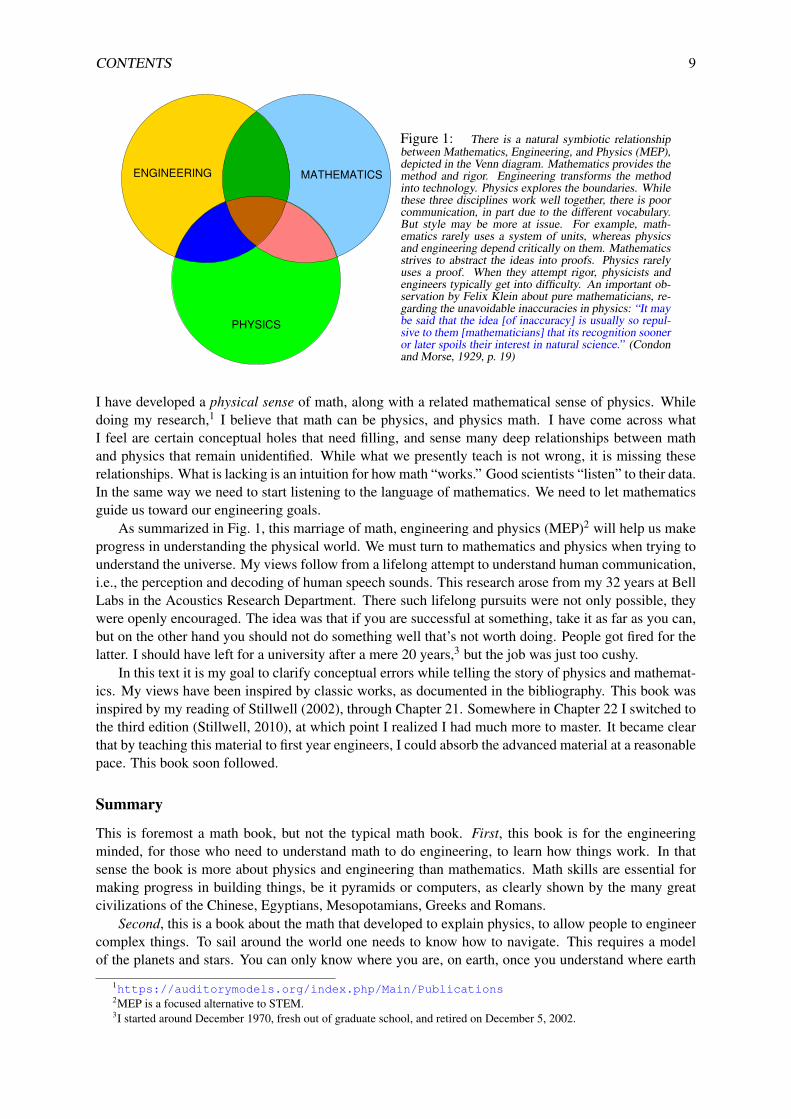
Figure 1: There is a natural symbiotic relationshipbetween Mathematics, Engineering, and Physics (MEP),depicted in the Venn diagram. Mathematics provides themethod and rigor. Engineering transforms the methodinto technology. Physics explores the boundaries. Whilethese three disciplines work well together, there is poorcommunication, in part due to the different vocabulary.But style may be more at issue. For example, math-ematics rarely uses a system of units, whereas physicsand engineering depend critically on them. Mathematicsstrives to abstract the ideas into proofs. Physics rarelyuses a proof. When they attempt rigor, physicists andengineers typically get into difficulty. An important ob-servation by Felix Klein about pure mathematicians, re-garding the unavoidable inaccuracies in physics: “It maybe said that the idea [of inaccuracy] is usually so repul-sive to them [mathematicians] that its recognition sooneror later spoils their interest in natural science.” (Condonand Morse, 1929, p. 19)
I have developed a physical sense of math, along with a related mathematical sense of physics. Whiledoing my research,1 I believe that math can be physics, and physics math. I have come across whatI feel are certain conceptual holes that need filling, and sense many deep relationships between mathand physics that remain unidentified. While what we presently teach is not wrong, it is missing theserelationships. What is lacking is an intuition for how math “works.” Good scientists “listen” to their data.In the same way we need to start listening to the language of mathematics. We need to let mathematicsguide us toward our engineering goals.
As summarized in Fig. 1, this marriage of math, engineering and physics (MEP)2 will help us makeprogress in understanding the physical world. We must turn to mathematics and physics when trying tounderstand the universe. My views follow from a lifelong attempt to understand human communication,i.e., the perception and decoding of human speech sounds. This research arose from my 32 years at BellLabs in the Acoustics Research Department. There such lifelong pursuits were not only possible, theywere openly encouraged. The idea was that if you are successful at something, take it as far as you can,but on the other hand you should not do something well that’s not worth doing. People got fired for thelatter. I should have left for a university after a mere 20 years,3 but the job was just too cushy.
In this text it is my goal to clarify conceptual errors while telling the story of physics and mathemat-ics. My views have been inspired by classic works, as documented in the bibliography. This book wasinspired by my reading of Stillwell (2002), through Chapter 21. Somewhere in Chapter 22 I switched tothe third edition (Stillwell, 2010), at which point I realized I had much more to master. It became clearthat by teaching this material to first year engineers, I could absorb the advanced material at a reasonablepace. This book soon followed.
Summary
This is foremost a math book, but not the typical math book. First, this book is for the engineeringminded, for those who need to understand math to do engineering, to learn how things work. In thatsense the book is more about physics and engineering than mathematics. Math skills are essential formaking progress in building things, be it pyramids or computers, as clearly shown by the many greatcivilizations of the Chinese, Egyptians, Mesopotamians, Greeks and Romans.
Second, this is a book about the math that developed to explain physics, to allow people to engineercomplex things. To sail around the world one needs to know how to navigate. This requires a modelof the planets and stars. You can only know where you are, on earth, once you understand where earth
1https://auditorymodels.org/index.php/Main/Publications2MEP is a focused alternative to STEM.3I started around December 1970, fresh out of graduate school, and retired on December 5, 2002.

10 CONTENTS
is, relative to the sun, planets, Milky Way and the distant stars. The answer to such a cosmic questiondepends strongly on who you ask. Who is qualified to answer such a question? It is best answered bythose who study mathematics applied to the physical world. The utility and accuracy of that answerdepends critically on the depth of understanding of the physics of the cosmic clock.
The English astronomer Edmond Halley (1656–1742) asked Newton (1643–1727) for the equationthat describes the orbit of the planets. Halley was obviously interested in comets. Newton immediatelyanswered “an ellipse.” It is said that Halley was stunned by the response (Stillwell, 2010, p. 176), as thiswas what had been experimentally observed by Kepler (c1619), and thus he knew Newton must havesome deeper insight. Both were eventually knighted.
When Halley asked Newton to explain how he knew, Newton responded “I calculated it.” But whenchallenged to show the calculation, Newton was unable to reproduce it. This open challenge eventuallyled to Newton’s grand treatise, Philosophiae Naturalis Principia Mathematica (July 5, 1687). It hada humble beginning, as a letter to Halley, explaining how to calculate the orbits of the planets. To dothis Newton needed mathematics, a tool he had mastered. It is widely accepted that Isaac Newton andGottfried Leibniz invented calculus. But the early record shows that perhaps Bhaskara II (1114–1185CE) had mastered the art well before Newton.4
Third, the main goal of this book is to teach motivated engineers mathematics, in a way that it canbe understood, mastered and remembered. How can this impossible goal be achieved? The answer is tofill in the gaps with Who did what, and when? Compared with the math, the historical record is easilymastered.
To be an expert in a field, one must know its history. This includes who the people were, whatthey did, and the credibility of their story. Do you believe the Pope or Galileo on the roles of the sunand the earth? The observables provided by science are clearly on Galileo’s side. Who were those firstengineers? They are names we all know: Archimedes, Pythagoras, Leonardo da Vinci, Galileo, Newton,etc. All of these individuals had mastered mathematics. This book presents the tools taught to everyengineer. Rather than memorizing complex formulas, make the relations “obvious” by mastering eachsimple underlying concept.
Fourth, when most educators look at this book, their immediate reactions are: Each lecture is atopic we spend a week on (in our math/physics/engineering class). And: You have too much materialcrammed into one semester. The first sentence is correct, the second is not. Tracking the students whohave taken the course, looking at their grades, and interviewing them personally, demonstrate that thematerial presented here is appropriate for one semester.5
To write this book I had to master the language of mathematics. I had already mastered the languageof engineering, and a good part of physics. One of my secondary goals is to build this scientific Towerof Babel, by unifying the terminology and removing the jargon.
Acknowledgments
I would like to acknowledge John Stillwell for his brilliant and constructive, historical summary of math-ematics, and my close friend and long-time (40 years) colleague Steve Levinson, who somehow drewme into this project, without my even knowing it. Next my brilliant graduate student Sarah Robinsonwas constantly at my side, first repairing blunders in my first-draft homeworks, and then grading theseand the exams, and tutoring the students. Without her, I would never have survived the first semesterthe material was taught. Her proofreading skills are amazing. Thank you Sarah for your infinite help.Without Kevin Pitts this never could have been started, as he provided early funding when the projectwas a germ of an idea. Matt Ando’s (Math) and Michael Stone’s (Physics) encouragement was psycho-logically important, in helping me think I might actually write a book. Finally I would like to thank JohnD’Angelo for his highly critical comments, due to my thousands of silly math questions. When it comesto the heavy hitting, John was always there to provide a brilliant explanation that I could easily translate
4http://www-history.mcs.st-and.ac.uk/Projects/Pearce/Chapters/Ch8_5.html5http://www.istem.illinois.edu/news/jont.allen.html

CONTENTS 11
into Engineerese (Matheering?) (i.e., engineer language).My delightful friend Robert Fossum, emeritus professor of mathematics from the University of Illi-
nois, kindly pointed out flawed mathematical terminology. James (Jamie) Hutchinson’s precise use ofthe English language dramatically raised the bar on my more than occasionally casual writing style. Toeach of you, thank you!
Finally I would like to thank my wife Sheau Feng Jeng, aka Patricia Allen, for her unbelievablesupport and love. She delivered constant peace of mind, without which this project could never havebeen started, much less finished. Many others (e.g., many students) played important roles, but giventheir large numbers, sadly they must remain anonymous.
–Jont Allen, Mahomet IL, May. 12, 2019

12 CONTENTS

Chapter 1
Introduction
Much of early mathematics dating before 1600 BCE centered around the love of art and music, dueto the sensations of light and sound. Our psychological senses of color and pitch are determined bythe frequencies (i.e., wavelengths) of light and sound. The Chinese and later the Pythagoreans are wellknown for their early contributions to music theory. We are largely ignorant of exactly what the Chinesescholars knew. The best record comes from Euclid, who lived in the 3rd century, after Pythagoras. Thuswe can only trace the early mathematics back to the Pythagoreans in the 6th century (580-500 BCE),which is centered around the Pythagorean theorem and early music theory.
Pythagoras strongly believed that “all is number,” meaning that every number, and every mathemat-ical and physical concept, could be explained by integral (integer) relationships, mostly based on eitherratios, or the Pythagorean theorem. It is likely that his belief was based on Chinese mathematics fromthousands of years earlier. It is also believed that his ideas about the importance of integers followedfrom the theory of music. The musical notes (pitches) obey natural integral ratio relationships, basedon the octave (a factor of two in frequency). The western 12-tone scale breaks the octave into 12 ratioscalled semitones. Today this has been rationalized to be the 12 root of 2, which is approximately equalto 18/17 ≈ 1.06 or 0.0833 octaves. This innate sense of frequency ratios comes from the physiologyof the auditory organ (the cochlea) which represents a fix distance along the Organ of Corti, the sensoryorgan of the inner ear.
As acknowledged by Stillwell (2010, p. 16), the Pythagorean view is relevant today:
With the digital computer, digital audio, and digital video coding everything, at least ap-proximately, into sequences of whole numbers, we are closer than ever to a world in which“all is number.”
1.1 Early science and mathematics
While early Asian mathematics has been lost, it clearly defined the course for math for at least severalthousand years. The first recorded mathematics were those of the Chinese (5000-1200 BCE) and theEgyptians (3,300 BCE). Some of the best early records were left by the people of Mesopotamia (Iraq,1800 BCE).1 While the first 5,000 years of math are not well documented, but the basic record is clear,as outlined in Fig. 1.1 (p. 15).
Thanks to Euclid, and later Diophantus (c250 CE), we have some basic (but vague) understanding ofChinese mathematics. For example, Euclid’s formula (Eq. 2.3, p. 56) provides a method for computingPythagorean triplets, a formula believed to be due to the Chinese.2
Chinese bells and stringed musical instruments were exquisitely developed with tonal quality, asdocumented by ancient physical artifacts (Fletcher and Rossing, 2008). In fact this development wasso rich that one must ask why the Chinese failed to initiate the industrial revolution. Specifically, why
1See Fig. 2.7, p. 57.2One might reasonably view Euclid’s role as that of a mathematical messenger.
13
14 CHAPTER 1. INTRODUCTION
did Europe eventually dominate with its innovation when it was the Chinese who did the extensive earlyinvention?
It could have been for the wrong reasons, but perhaps our best insight into the scientific history fromChina may have come from an American chemist and scholar from Yale, Joseph Needham, who learnedto speak Chinese after falling in love with a Chinese woman, and ended up researching early Chinesescience and technology for the US government.
According to Lin (1995) this is known as the Needham question:
“Why did modern science, the mathematization of hypotheses about Nature, with all itsimplications for advanced technology, take its meteoric rise only in the West at the time ofGalileo[, but] had not developed in Chinese civilization or Indian civilization?”
Needham cites the many developments in China:
“Gunpowder, the magnetic compass, and paper and printing, which Francis Bacon consid-ered as the three most important inventions facilitating the West’s transformation from theDark Ages to the modern world, were invented in China.” (Lin, 1995; Apte, 2009)
“Needham’s works attribute significant weight to the impact of Confucianism and Taoismon the pace of Chinese scientific discovery, and emphasize what it describes as the ‘diffu-sionist’ approach of Chinese science as opposed to a perceived independent inventivenessin the western world. Needham held that the notion that the Chinese script had inhibitedscientific thought was ‘grossly overrated’ ” (Grosswiler, 2004).
Lin (1995) was focused on military applications, missing the importance of non-military contribu-tions. A large fraction of mathematics was developed to better understand the solar system, acoustics,musical instruments and the theory of sound and light. Eventually the universe became a popular topic,as it still is today.
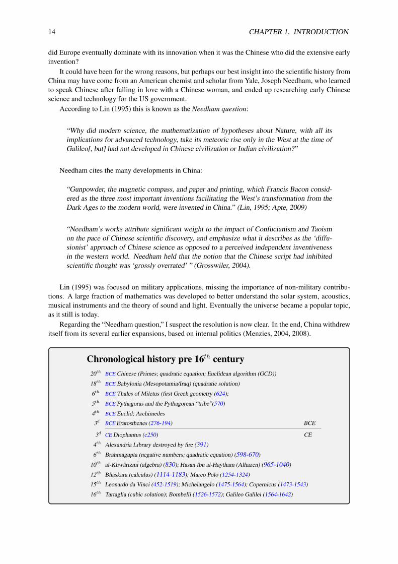
Regarding the “Needham question,” I suspect the resolution is now clear. In the end, China withdrewitself from its several earlier expansions, based on internal politics (Menzies, 2004, 2008).
Chronological history pre 16th century20th BCE Chinese (Primes; quadratic equation; Euclidean algorithm (GCD))
18th BCE Babylonia (Mesopotamia/Iraq) (quadratic solution)
6th BCE Thales of Miletus (first Greek geometry (624);
5th BCE Pythagoras and the Pythagorean “tribe”(570)
4th BCE Euclid; Archimedes
3d BCE Eratosthenes (276-194) BCE
3d CE Diophantus (c250) CE
4th Alexandria Library destroyed by fire (391)
6th Brahmagupta (negative numbers; quadratic equation) (598-670)
10th al-Khwarizmi (algebra) (830); Hasan Ibn al-Haytham (Alhazen) (965-1040)
12th Bhaskara (calculus) (1114-1183); Marco Polo (1254-1324)
15th Leonardo da Vinci (452-1519); Michelangelo (1475-1564); Copernicus (1473-1543)
16th Tartaglia (cubic solution); Bombelli (1526-1572); Galileo Galilei (1564-1642)

1.1. EARLY HISTORY 15
1.1.1 The Pythagorean theorem
Thanks to Euclid’s Elements (c323 BCE) we have an historical record, tracing the progress in geometry,as established by the Pythagorean theorem, which states that for any right triangle having sides oflengths (a, b, c) ∈ R that are either positive real numbers, or more interesting, integers c > [a, b] ∈ Nsuch that a+ b > c,
c2 = a2 + b2. (1.1)
Early integer solutions were likely found by trial and error rather than by an algorithm.
1500BCE |0CE |500 |1000 |1400 |1650
|830Caeser
ChineseBabylonia
PythagoreansEuclid
LeonardoBrahmaguptaDiophantus Bhaskara
ArchimedesBombelli
al-KhawarizmiMarco Polo
Copernicus
Figure 1.1: Mathematical timeline between 1500 BCE and 1650 CE. The western renaissance is considered to have occurredbetween the 15th and 17th centuries. However, the Asian “renaissance” was likely well before the 1st century (i.e., 1500 BCE).There is significant evidence that a Chinese ‘treasure ship’ visited Italy in 1434, initiating the Italian renaissance (Menzies,2008). This was not the first encounter between the Italians and the Chinese, as documented in ‘The travels of Marco Polo’(c1300 CE).
If a, b, c are lengths, then a2, b2, c2 are each the area of a square. Equation 1.1 says that the area a2
plus the area b2 equals the area c2. Today a simple way to prove this is to compute the magnitude of thecomplex number c = a+ b, which forces the right angle
|c|2 = (a+ b)(a− b) = a2 + b2. (1.2)
However, complex arithmetic was not an option for the Greek mathematicians, since complex numbersand algebra had yet to be discovered.
Almost 700 years after Euclid’s Elements, the Library of Alexandria was destroyed by fire (391CE), taking with it much of the accumulated Greek knowledge. As a result, one of the best technicalrecords remaining is Euclid’s Elements, along with some sparse mathematics due to Archimedes (c300BCE) on geometrical series, computing the volume of a sphere, the area of the parabola, and elementaryhydrostatics. In c1572 a copy Diophantus’s Arithmetic was discovered by Bombelli in the Vatican library(Burton, 1985; Stillwell, 2010, p. 51). This book became an inspiration for Galileo, Descartes, Fermatand Newton.
Early number theory: Well before Pythagoras, the Babylonians (c1,800 BCE) had tables of tripletsof integers [a, b, c] that obey Eq. 1.1, such as [3, 4, 5]. However, the triplets from the Babylonians werelarger numbers, the largest being a = 12709, c = 18541. A stone tablet (Plimpton-322) dating backto 1800 BCE was found with integers for [a, c] (). Given such sets of two numbers, which determineda third positive integer b = 13500 such that b =
√c2 − a2, this table is more than convincing that the
Babylonians were well aware of Pythagorean triplets (PTs), but less convincing that they had access toEuclid’s formula, a formula for PTs. (Eq. 2.3 p. 56).
It seems likely that Euclid’s Elements was largely the source of the fruitful era due to the Greekmathematician Diophantus (215-285) (Fig. 1.1), who developed the field of discrete mathematics nowknown as Diophantine analysis. The term means that the solution, not the equation, is integer. The workof Diophantus was followed by fundamental change in mathematics, possibly leading to the developmentof algebra, but at least including the discovery of
1. negative numbers,
2. quadratic equation (Brahmagupta, 7th CE),

16 CHAPTER 1. INTRODUCTION
3. algebra (al-Khwarizmi, 9th CE), and
4. complex arithmetic (Bombelli, 15th CE).
These discoveries overlapped with the European middle (aka, dark) ages. While Europe went “dark,”presumably European intellectuals did not stop working during these many centuries.3
1.1.2 What is science?
Science is a process to quantify hypotheses to build truths. Today it has evolved from the early Greekphilosophers, Plato and Aristotle, to a statistical method to either validate or prove wrong, the nullhypothesis, using statistical tests. Scientists use the term “null hypothesis” to describe the suppositionthat there is no difference between the two intervention groups or “no effect” of a treatment on somemeasured outcome. This measure of the likelihood that an obtained value occurred by chance is calledthe “p-value,” which when small gives confidence that the null hypothesis is either true (no differenceinduced by the treatment variables) or faults (above chance effect induced by the treatment variables ofprobability p). While the present standard of scientific truth, it is not iron clad, and must be used withcaution. For example, not all experimental tests may be reduced to a single binary test. Does the sunrotate around the moon, or around the earth? There is no test of this question, as it is nonsense. To evensay that the earth rotates around the sun is, in some sense nonsense, because all the planets are involvedin the many motions.
Yet science works quite well. We have learned many deep secrets regarding the universe over thelast 5,000 years.
1.1.3 What is mathematics?
It seems strange when people complain they “can’t learn math,”4 but then claim to be good at languages.Pre-high-school students tend to confuse arithmetic with math. One does not need to be good at arith-metic to be good at math (but it doesn’t hurt). Gauss made his career based on numbers, especiallyprimes.
Math is a language, with the symbols taken from various languages, not so different from otherlanguages. Today’s mathematics is a written language with an emphasis on symbols and glyphs, biasedtoward Greek letters, obviously due to the popularity of Euclid’s Elements. The specific evolution ofthese symbols is interesting (Mazur, 2014). Each symbol is dynamically assigned a meaning, appropri-ate for the problem being described. These symbols are then assembled to make sentences. It is similarto Chinese in that the spoken and written versions are different across dialects. Like Chinese, the sen-tences may be read out loud in any language (dialect), while the mathematical sentence (like Chinesecharacters) is universal.
Learning languages is an advanced social skill. However, the social outcomes of learning a languageand learning math are very different. Learning a new language is fun because it opens doors to othercultures. Math is different due to the rigor of the grammer (rules of the language), along with the wayit is taught (e.g., not as a language). A third difference between math and language is that math evolvedfrom physics, with important technical applications.
As with any language, the more mathematics you learn, the easier it is to understand, because math-ematics is built from the bottom up. It’s a continuous set of concepts, much like the construction of ahouse. If you try to learn calculus and differential equations, while skipping simple number theory, thelessons will be more difficult to understand. You will end up memorizing instead of understanding, andas a result you will likely soon forget it. When you truly understand something, it can never be forgotten.A nice example is the solution to a quadratic equation: If you learn how to complete the square (p. 73),you will never forget the quadratic formula.
3It would be interesting to search the archives of the monasteries, where the records were kept, to determine exactly whathappened during this religious blackout.
4“It looks like Greek to me.”

1.1. EARLY HISTORY 17
The topics need to be learned in order, just as in the case of building the house. You can’t builda house if you don’t know about screws or cement (plaster). Likewise in mathematics, you will notlearn to integrate if you have failed to understand the difference between integers, complex numbers,polynomials, and their roots.
A short list of topics for mathematics are numbers (N,Z,Q, I,C), algebra, derivatives, anti-derivatives(i.e., integration), differential equations, vectors and the spaces they define, matrices, matrix algebra,eigenvalues and vectors, solutions of systems of equations, matrix differential equations and their eigen-solution. Learning is about understanding, not memorizing.
The rules of mathematics are formally defined by algebra. For example, the sentence a = b meansthat the number a has the same value as the number b. The sentence is spoken as “a equals b.” Thenumbers are nouns and the equal sign says they are equivalent, playing the role of a verb, or actionsymbol. Following the rules of algebra, this sentence may be rewritten as a− b = 0. Here the symbolsfor minus and equal indicate two types of actions (verbs).
Sentences can become arbitrarily complex, such as the definition of the integral of a function, ora differential equation. But in each case, the mathematical sentence is written down, may be read outloud, has a well-defined meaning, and may be manipulated into equivalent forms following the rules ofalgebra and calculus. This language of mathematics is powerful, with deep consequences, first knownas algorithms, but eventually as theorems.
The writer of an equation should always translate (explicitly summarize the meaning of the expres-sion), so the reader will not miss the main point, as a simple matter of clear writing.
Just as math is a language, so language may be thought of as mathematics. To properly writecorrect English it is necessary to understand the construction of the sentence. It is important to identifythe subject, verb, object, and various types of modifying phrases. Look up the interesting distinctionbetween that and which.5 Thus, like math, language has rules. Most individuals use what “soundsright,” but if you’re learning English as a second language, it is necessary to understand the rules, whichare arguably easier to master than the foreign speech sounds.
Context can be critical, and the most important context for mathematics is physics. Without a phys-ical problem to solve, there can be no engineering mathematics. People needed to navigate the earth,and weigh things. This required an understand of gravity. Many questions about gravity were deep,such as “Where is the center of the universe?”6 But church dogma only goes so far. Mathematics, alongwith a heavy dose of physics, finally answered this huge question. Someone needed to perfect the tele-scope, and put satellites into space, and view the cosmos. Without mathematics none of this would havehappened.
|1526 |1596 |1650 |1700 |1750 |1800 |1850
Daniel Bernoulli
Euler
dAlembert
Gauss
Cauchy
LagrangeNewton
Descartes
Fermat
Galileo
Johann BernoulliBombelli
Figure 1.2: Timeline covering the two centuries from 1596CE to 1855CE, covering the development of the modern theoriesof analytic geometry, calculus, differential equations and linear algebra. Newton was born about 1 year after Galileo diedand thus was heavily influenced by his many discoveries. The vertical red lines indicate mentor-student relationships. Notethe significant overlap between Newton and Johann and his son Daniel Bernoulli, and Euler, a nucleation point for modernmathematics. Gauss had the advantage of input from Newton, Euler, d’Alembert and Lagrange. Lagrange had a key role in thedevelopment of linear algebra. Likely Cauchy had a significant contemporary influence on Gauss as well. Finally, note thatFig. 1.1 ends with Bombelli while this figure begins with him. He was a mathematician who famously discovered a copy ofDiophantus’ book in the Vatican library. This was the same book that Fermat wrote in, for which the margin was too small tohold the “proof” of his “last theorem.”
5https://en.oxforddictionaries.com/usage/that-or-which6Actually this answer is simple: Ask the Pope and he will tell you. (I apologize for this inappropriate joke.)

18 CHAPTER 1. INTRODUCTION
1.1.4 Early physics as mathematics: Back to Pythagoras
There is a second answer to the question What is mathematics? The answer comes from studying itshistory, which starts with the earliest record. This chronological view starts, of course, with the studyof numbers. First there is the taxonomy of numbers. It took thousands of years to realize that numbersare more than the counting numbers N, and to create a symbol for nothing (i.e., zero), and to inventnegative numbers. With the invention of the abacus, a memory aid for the manipulation of complex setsof real integers, one could do very detailed calculations. But this required the discovery of algorithms(procedures) to add, subtract, multiply (many adds of the same number) and divide (many subtractsof the same number), such as the Euclidean algorithm for the GCD. Eventually it became clear to theexperts (early mathematicians) that there were natural rules to be discovered, thus books (e.g., Euclid’sElements) were written to summarize this knowledge.
The role of mathematics is to summarize algorithms (i.e., sets of rules), and formalize the idea as atheorem. Pythagoras and his followers, the Pythagoreans, believed that there was a fundamental relation-ship between mathematics and the physical world. The Asian civilizations were the first to capitalize onthe relationship between science and mathematics, to use mathematics to design things for profit.Thismay have been the beginning of capitalizing technology (i.e., engineering), based on the relationshipbetween physics and math. This impacted commerce in many ways, such as map making, tools, imple-ments of war (the wheel, gunpowder), art (music), water transport, sanitation, secure communication,food, etc. Of course the Chinese were among the first to master many of these technologies.
Why is Eq. 1.1 called a theorem? Theorems require a proof. What exactly needs to be proved? Wedo not need to prove that (a, b, c) obey this relationship, since this is a condition that is observed. Wedo not need to prove that a2 is the area of a square, as this is the definition of an area. What needs to beproved is that the relation c2 = a2 + b2 holds if, and only if, the angle between the two shorter sides is90. The Pythagorean theorem (Eq. 1.1) did not begin with Euclid or Pythagoras, rather they appreciatedits importance, and documented its proof.
In the end the Pythagoreans, who instilled fear in the neighborhood, were burned out, and murdered,likely the fate of mixing technology with politics:
“Whether the complete rule of number (integers) is wise remains to be seen. It is said thatwhen the Pythagoreans tried to extend their influence into politics they met with popularresistance. Pythagoras fled, but he was murdered in nearby Mesopotamia in 497 BCE.”
–Stillwell (2010, p. 16)
1.2 Modern mathematics is born
Modern mathematics (what we practice today) was born in the 15-16th centuries, in the minds ofLeonardo da Vinci, Bombelli, Galileo, Descartes, Fermat, and many others (Burton, 1985). Many ofthese early masters were, like the Pythagoreans, secretive to the extreme about how they solved prob-lems. This soon changed due to Galileo, Mersenne, Descartes and Newton, causing mathematics toblossom. The developments during this time may seemed hectic and disconnected. But this is a wrongimpression, as the development was dependent on new technologies such as the telescope (optics) andmore accurate time and frequency measurements, due to Galileo’s studies of the pendulum, and a betterunderstanding of the relation fλ = co between frequency f , wavelength λ and the wave speed co.
1.2.1 Science meets mathematics
Galileo: In 1589 Galileo famously conceptualized an experiment where he suggested dropping twodifferent weights from the Leaning Tower of Pisa, and he suggested that they must take the same timeto hit the ground.
Conceptually this is a mathematically sophisticated experiment, driven by a mathematical argumentin which he considered the two weights to be connected by an elastic cord (a spring) or balls rolling

1.2. MODERN MATHEMATICS IS BORN 19
Mass
Mass
Spring
Mass
Mass
t = 0
t = 1
Figure 1.3: Depiction of the argument of Galileo (unpublished book of 1638) as to why weights of different masses (i.e.,weight) must fall with the same velocity, contrary to what Archimedes had proposed c250 BCE.
down a friction-less incline plane. His studies resulted in the concept of conservation of energy, one ofthe cornerstones of physical theory since that time.
Being joined with an elastic cord, the masses become one. If the velocity were proportional to themass, as believed by Archimedes, the sum of the two weights would necessarily fall even faster. Thisresults in a logical fallacy: How can two masses fall faster than either? This also violates the concept ofconservation of energy, as the total energy of two masses would be greater than that of the parts. In factGalileo’s argument may have been the first time that the principle of conservation of energy was clearlystated.
It seems likely that Galileo was attracted to this model of two masses connected by a spring becausehe was also interested in planetary motion, which consist of masses (sun, earth, moon), also mutuallyattracted by gravity (i.e., the spring).
Galileo also performed related experiments on pendulums, where he varied the length l, massm, andangle θ of the swing. By measuring the period (periods/unit time) he was able to formulate precise rulesbetween the variables. This experiment also measured the force exerted by gravity, so the experimentswere related, but in very different ways. The pendulum served as the ideal clock, as it needed very littleenergy to keep it going, due to its very low friction (energy loss).
In a related experiment, Galileo measured the duration of a day by counting the number of swingsof the pendulum in 24 hours, measured precisely by the daily period of a star as it crossed the tip ofa church steeple. The number of seconds in a day is 24×60×60 = 86400 = 273352 [s/day]. Since86,400 is the product of the first three primes, it is highly composite, and thus may be reduced in manyequivalent ways. For example, the day can be divided evenly into 2, 3, 5 or 6 parts, and remain exactin terms of the number of seconds that transpire. Factoring the number of days in a year (365=5*73)is not useful, since it may not be decomposed into many small primes.7 Galileo also extended workon the relationship of wavelength and frequency of a sound wave in musical instruments. On top ofthese impressive accomplishments, Galileo greatly improved the telescope, which he needed for hisobservations of the planets.
Many of Galileo’s contributions resulted in new mathematics, leading to Newton’s discovery of thewave equation (c1687), followed 60 years later by its one-dimensional general solution by d’Alembert(c1747).
Mersenne: Marin Mersenne (1588–1648) also contributed to our understanding of the relationshipbetween the wavelength and the dimensions of musical instruments, and is said to be the first to mea-sure the speed of sound. At first Mersenne strongly rejected Galileo’s views, partially due to errors in
7For example, if the year were 364 = 22 · 7 · 13 days, it would would make for shorter years (by 1 day), 13 months peryear (e.g., 28 = 2 · 2 · 7 day vacation per year?), perfect quarters, and exactly 52 week. Every holiday would always fall onthe same day, every year. It would be a calendar that humans could understand.

20 CHAPTER 1. INTRODUCTION
Galileo’s reports of his results. But once Mersenne saw the significance of Galileo’s conclusion, hebecame Galileo’s strongest advocate, helping to spread the word (Palmerino, 1999).
This incident invokes an important theorem of nature: Is data more like bread or wine? The answeris, it depends on the data. Galileo’s original experiments on pendulums and ball falling down slopes,were flawed by inaccurate data. This is likely because he didn’t have good clocks. But he soon solvedthat problem and the data became more accurate. We don’t know if Mersenne repeated Galileo’s exper-iments, and then appreciated his theory, or if he communicated with Galileo. But the final resolutionwas that the early data were like bread (it rots), but when the experimental method was improved, with abetter clock, the corrected data was like wine (which improves with age). Galileo claimed that the timefor the mass to drop a fixed distance was exactly proportional to the square of the time. This expressionlead to F = ma. One follows from the other. If the mass varies then you get Newton’s second law ofmotion (Eq. 3.2, p. 70).
He was also a decent mathematician, inventing (1644) the Mersenne primes (MP) πm of the form
πm = 2πk − 1,
where πk (k < m) denotes the kth prime (p. 26). As of Dec 2018 51 MPs are known.8 The first MP is3 = π2 = 2π1 − 1, and the largest known prime is a MP. Note that 127 = π31 = 2π7 − 1 is the MP ofthe MP π7.
Newton: With the closure of Cambridge University due to the plague of 1665, Newton returned hometo Woolsthorpe-by-Colsterworth (95 [mi] north of London), to work by himself for over a year. It wasduring this solitary time that he did his most creative work.
While Newton (1642–1726) may be best known for his studies on light and gravity, he was the firstto predict the speed of sound. However, his theory was in error9 by
√cp/cv =
√1.4 = 1.183. This
famous error would not be resolved for 140 years, awaiting the formulation of thermodynamics and theequi-partition theorem by Laplace in 1816 (Britannica, 2004).
Just 11 years prior to Newton’s 1687 Principia, there was a basic understanding that sound andlight traveled at very different speeds, due to the experiments of Ole Rømer (Feynman, 1968; Feynman:Speed of Light, 2019, google online Feynman videos)
Ole Rømer first demonstrated in 1676 that light travels at a finite speed (as opposed toinstantaneously) by studying the apparent motion of Jupiter’s moon Io. In 1865, JamesClerk Maxwell proposed that light was an electromagnetic wave, and therefore traveledat the speed co appearing in his theory of electromagnetism (Wikipedia: Speed of Light,2019).
The idea behind Rømer’s discovery was that due to the large distance between Earth and Io, therewas a difference between the period of the moon when Jupiter was closest to Earth vs. when it wasfarthest from Earth. This difference in distance caused a delay or advance in the observed eclipse of Ioas it went behind Jupiter, delayed by the difference in time due to the difference in distance. It is likewatching a video of a clock, delayed or sped up. When the video is either delayed or slowed down, thetime will be inaccurate (it will indicate an earlier time).
Studies of vision and hearing: Since light and sound (music) played such a key role in the develop-ment of the early science, it was important to fully understand the mechanism of our perception of lightand sound. There are many outstanding examples where physiology impacted mathematics. Leonardoda Vinci (1452–1519) is well known for his early studies of the human body. Exploring our physio-logical senses requires a scientific understanding of the physical processes of vision and hearing, first
8http://mathworld.wolfram.com/MersennePrime.html9The square root of the ratio of the specific heat capacity at constant pressure cp to that at constant volume cv .

1.2. MODERN MATHEMATICS IS BORN 21
Figure 1.4: Above left: Jakob (1655–1705) and right: Johann (1667–1748) Bernoulli, both painted by their portrait painterbrother, Nicolaus. Below left: Leonhard Euler (1707-1783) and right: Jean le Rond d’Alembert (1717-1783). Euler was blindin his right eye, hence the left portrait view.

22 CHAPTER 1. INTRODUCTION
considered by Newton (1687) (1643–1727), but first properly researched much later by Helmholtz (Still-well, 2010, p. 261). Helmholtz’s (1821–1894) studies and theories of music and the perception of soundare fundamental scientific contributions (Helmholtz, 1863a). His best known mathematical contributionis today known as the fundamental theorem of vector calculus, or simply Helmholtz theorem (p. 231).
The amazing Bernoulli family: The first individual who seems to have openly recognized the impor-tance of mathematics, enough to actually teach it, was Jacob Bernoulli (1654–1705) (Fig. 1.4). Jacobworked on what is now viewed as the standard package of analytic “circular” (i.e., periodic) functions:sin(x), cos(x), exp(x), log(x).10 Eventually the full details were developed (for real variables) byEuler (p. 91).
From Fig. 1.2 (p. 17) we see that Jacob was contemporary with Descartes, Fermat, and Newton. Thusit seems likely that he was strongly influenced by Newton, who in turn was influenced by Descartes11
(White, 1999). Vite and Wallis, but mostly by Galileo, who died 1 year before Newton was born, onChristmas day 1642. Because the calendar was modified during Newton’s lifetime, his birth date is nolonger given as Christmas (Stillwell, 2010, p. 175).
Jacob Bernoulli, like all successful mathematicians of the day, was largely self-taught. Yet Ja-cob was in a new category of mathematicians because he was an effective teacher. Jacob taught hissibling Johann (1667–1748), who then taught his sibling Daniel (1700–1782). But most importantly,Johann taught Leonhard Euler (1707–1783), the most prolific (thus influential) of all mathematicians.This teaching resulted in an explosion of new ideas and understanding. It is most significant that allfour mathematicians published their methods and findings. Much later, Jacob studied with students ofDescartes12 (Stillwell, 2010, p. 268-9).
Euler: Euler’s mathematical talent went far beyond that of the Bernoulli family (Burton, 1985). An-other special strength of Euler was the degree to which he published. First he would master a topic, andthen he would publish. His papers continued to appear long after his death (Calinger, 2015). It is alsosomewhat interesting that Leonhard Euler was a contemporary of Mozart (and James Clerk Maxwell ofAbraham Lincoln Fig. 1.5, p. 23).
d’Alembert: Another individual of that time of special note, who also published extensively, wasd’Alembert (Fig. 1.4). Some of the most innovative ideas were first proposed by d’Alembert. Unfortu-nately, and perhaps somewhat unfairly, his rigor was criticized by Euler, and later by Gauss (Stillwell,2010). But once the tools of mathematics were finally openly published, largely by Euler, mathematicsgrew exponentially.13
Gauss: Figure 1.2 (p. 17) shows the timeline of the most famous mathematicians. It was one of themost creative times in mathematics. Gauss was born at the end of Euler’s long and productive life.I suspect that Gauss owed a great debt to Euler: surely he must have been a scholar of Euler. One ofGauss’s most important achievements may have been his contribution to solving the open question aboutthe density of prime numbers and his use of least-squares.14
Cauchy: Augustin-Louis Cauchy (1760–1848), Fig. 1.2 (p. 17), was the son of a well todo family, buthad the misfortune of being born during the time of of the French revolution, which perhaps started withthe seven years war which began around 1756. Today the French celebrate Bestial day, July 14 1789,
10The log and tan functions are related by Eq. 4.2 p. 146.11http://www-history.mcs.st-andrews.ac.uk/Biographies/Newton.html12It seems clear that Descartes was also a teacher.13There are at least three useful exponential scales: Factors of 2, factors of e ≈ 2.7, and factors of 10. The octave and
decibel use factors of 2 (6 [dB]) and 10 (20 [dB]). Information theory uses powers of 2 (1 [bit]), 4 (2 [bits]). Circuit theoryuses all three.
14http://www-history.mcs.st-andrews.ac.uk/Biographies/Gauss.html.
1.2. MODERN MATHEMATICS IS BORN 23
which is viewed as a celebration of the revolution. The French revolution left Cauchy with a life-timestigma for French politics, that deeply influenced his life. But regardless of his scorn for French politics,he had an unmatched intellect for mathematics. His most obvious achievement was complex analysis,for which he proved many key theorems.
|1525 |1564 |1650 |1750 |1800 |1875 |1925
Lincoln
Napolean WWI
Mersenne
Fermat
HilbertDescartes
Mozart
Johann Bernoulli
Jacob BernoulliDaniel Bernoulli
EinsteinHuygens
Euler
Newton
d'Alembert
Cauchy
Galileo GaussHelmholtz
Maxwell
Riemann
Bombelli
Rayleigh
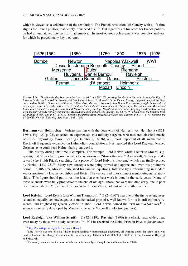
Figure 1.5: Timeline for the four centuries from the 16th and 20th CE covering Bombelli to Einstein. As noted in Fig. 1.2,it seems likely that Bombelli’s discovery of Diophantus’s book “Arithmetic” in the Vatican library, triggered many of the ideaspresented by Galileo, Descartes and Fermat, followed by others (i.e., Newton), thus Bombelli’s discovery might be consideredas a magic moment in mathematics. The vertical red lines indicate mentor-student relationships. For orientation, Mozart andLincoln are indicated along the bottom and Napoleon along the top. Napoleon hired Fourier, Lagrange and Laplace to helpwith his many bloody military campaigns. Related timelines include (see index): Fig. 1.1 (p. 15) which gives the timeline from1500 BCE to 1650 CE; Fig. 1.2 (p. 17) presents the period from Descartes to Gauss and Cauchy; Fig. 3.1 (p. 70) presents the17-20 CE (Newton–Einstein) view from 1640–1950;
Hermann von Helmholtz: Perhaps starting with the deep work of Hermann von Helmholtz (1821-1894), Fig. 1.5 (p. 23), educated an experienced as a military surgeon, who mastered classical music,acoustics, physiology, vision, hearing (Helmholtz, 1863b), and, most important of all, mathematics.Kirchhoff frequently expanded on Helmholtz’s contributions. It is reported that Lord Rayleigh learnedGerman so he could read Helmholtz’s great works.
The history during this time is complex. For example, Lord Kelvin wrote a letter to Stokes, sug-gesting that Stokes try to prove what is today known as “Stokes theorem.” As a result, Stokes posted areward (the Smith Prize), searching for a prove of “Lord Kelvin’s theorem,” which was finally provedby Hankel (1839-73).15 Many new concepts were being proved and appreciated over this productiveperiod. In 1863-65, Maxwell published his famous equations, followed by a reformatting in modernvector notation by Heaviside, Gibbs and Hertz. The vertical red lines connect mentor-student relation-ships. This figure should put to rest the idea that ones best work is done in the early years. Many ofthese scientists were fully productive to the end of old age. Those that were not, died early, due to poorhealth or accidents. Mozart and Beethoven are time-anchors, not part of the math timeline.
Lord Kelvin: Lord Kelvin (aka William Thompson),16 (1824-1907) was one of the first true engineer-scientists, equally acknowledged as a mathematical physicist, well known for his interdisciplinary re-search, and knighted by Queen Victoria in 1866. Lord Kelvin coined the term thermodynamics,17 ascience more fully developed by Maxwell (the same Maxwell of electrodynamics).
Lord Rayleigh (aka William Strutt): (1842-1919). Rayleigh (1896) is a classic text, widely readeven today by those who study acoustics. In 1904 he received the Nobel Prize in Physics for his inves-
15https://en.wikipedia.org/wiki/Hermann Hankel16Lord Kelvin was one of a half dozen interdisciplinary mathematical physicists, all working about the same time, who
made a fundamental change in our scientific understanding. Others include Helmholtz, Stokes, Green, Heaviside, Rayleighand Maxwell.
17Thermodynamics is another case which warrants an analysis along historical lines (Kuhn, 1978).

24 CHAPTER 1. INTRODUCTION
tigations of the densities of the most important gases and for his discovery of argon in connection withthese studies.
1.2.2 Three Streams from the Pythagorean theorem
From the outset of his presentation, Stillwell (2010, p. 1) defines “three great streams of mathematicalthought: Numbers, Geometry and Infinity” that flow from the Pythagorean theorem, as summarized inTable 1.1. This is a useful concept, based on reasoning not as obvious as one might think. Many factorsare in play here. One of these is the strongly held opinion of Pythagoras that all mathematics shouldbe based on integers. The rest are tied up in the long, necessarily complex history of mathematics, asbest summarized by the fundamental theorems (Box material 2.3.1, p. 38), each of which is discussed indetail in a relevant chapter.
Table 1.1: Three streams followed from Pythagorean theorem: number systems, geometry and infinity.
• The Pythagorean theorem is the mathematical spring which bore the three streams.
• Several centuries per stream:
1) Numbers:6thBCE N counting numbers, Q rationals, P primes5thBCE Z common integers, I irrationals
7thCE zero ∈ Z2) Geometry: (e.g., lines, circles, spheres, toroids, . . . )
17thCE Composition of polynomials (Descartes, Fermat)Euclid’s geometry & algebra⇒ analytic geometry
18thCE Fundamental theorem of algebra3) Infinity: (∞→ Sets)
17-18thCE Taylor series, functions, calculus (Newton, Leibniz)19thCE R real, C complex 185120thCE Set theory
As shown in the insert, Stillwell’s concept of three streams, following from the Pythagorean theorem,is the organizing principle behind this book.
1. The Introduction is intended to be a self-contained survey of basic pre-college mathematics, as adetailed overview of the fundamentals, presented as three main streams:
1) Number systems: (p. 25)
2) Algebraic equations: (p. 69)
3a) Scalar calculus: (p. 145)
3b) Vector calculus: (p. 187)
2. Number Systems Some uncertain ideas of number systems, starting with prime numbers, throughcomplex numbers, vectors and matrices.
3. Algebraic Equations Algebra and its development, as we know it today. The theory of real andcomplex equations and functions of real and complex variables. Complex impedance Z(s) ofcomplex frequency s = σ + ω is covered with some care, developing the topic which is neededfor engineering mathematics.
4. Scalar Calculus (Stream 3a) Ordinary differential equations. Integral theorems. Acoustics.
5. Vector Calculus: (Stream 3b) Vector partial differential equations. Gradient, divergence and curldifferential operators. Stokes’s and Green’s theorems. Maxwell’s equations.

Chapter 2
Stream 1: Number Systems
Number theory (the study of numbers) was a starting point for many key ideas. For example, in Euclid’sgeometrical constructions the Pythagorean theorem for real [a, b, c] was accepted as true, but the empha-sis in the early analysis was on integer constructions, such as Euclid’s formula for Pythagorean triplets(Eq. 2.3, Fig. 2.6, p. 56).
As we shall see, the derivation of the formula for Pythagorean triplets is the first of a rich sourceof mathematical constructions, such as solutions of Pell’s equation (p. 57),1 and the recursive differenceequations, such as solutions of the Fibonacci recursion formula fn+1 = fn + fn−1 (p. 59) which goesback at least to the Chinese (c2000 BCE). These are early pre-limit forms of calculus, best analyzedusing an eigen-function (e.g., eigen-matrix) expansion, a geometrical concept from linear algebra, as anorthogonal set of normalized unit-length vectors (Appendix B.3, p. 265).
The first use of zero and∞: It is hard to imagine that one would not appreciate the concept of zeroand negative numbers when using an abacus. It does not take much imagination to go from countingnumbers N to the set of all integers Z, including zero. On an abacus, subtraction is obviously the inverseof addition. Subtraction, to obtain zero abacus beads, is no different than subtraction from zero, givingnegative beads. To assume the Romans, who first developed counting sticks, or the Chinese who thendeployed the concept using beads, did not understand negative numbers, is impossible.
However, understanding the concept of zero (and negative numbers) is not the same as havinga symbolic notation. The Roman number system has no such symbols. The first recorded use ofa symbol for zero is said to be by Brahmagupta2 in 628 CE.3 However this is likely wrong, giventhe notation developed by the Mayan civilization which existed from 2000BCE to 900CE (https://www.storyofmathematics.com/mayan.html). There is speculation that the Mayans cut down somuch of the Amazon jungle that it eventually resulted in a global warming anomaly, possibly resultingin their demise.
Defining zero (c628 CE) depends on the concept of subtraction, which formally requires the creationof algebra (c830 CE, Fig. 1.1, p. 15). But apparently it takes more than 600 years, i.e., from the timeRoman numerals were put into use, without any symbol for zero, to the time when the symbol for zerois first documented. Likely this delay is more about the political situation, such as government rulings,than mathematics.
The concept that caused much more difficulty was ∞, first resolved by Riemann in 1851 with thedevelopment of the extended plane, which mapped the plane to a sphere (Fig. 3.14 p. 138). His con-struction made it clear that the point at ∞ is simply another point on the open complex plane, sincerotating the sphere (extended plane) moves the point at∞ to a finite point on the plane, thereby closing
1Heisenberg, an inventor of the matrix algebra form of quantum mechanics, learned mathematics by studying Pell’s equa-tion (p. 57) https://www.aip.org/history-programs/niels-bohr-library/oral-histories/4661-1 by eigen-vector and recursive analysis methods.
2http://news.nationalgeographic.com/2017/09/origin-zero-bakhshali-manuscript-video-spd/3https://www.nytimes.com/2017/10/07/opinion/sunday/who-invented-zero.html
25
26 CHAPTER 2. STREAM 1: NUMBER SYSTEMS
the complex plane.
2.1 The taxonomy of numbers: N,P,Z,Q,F, I,R,C
Once symbols for zero and negative numbers were accepted, progress could be made. To fully under-stand numbers, a transparent notation was required. First one must differentiate between the differentclasses (genus) of numbers, providing a notation that defines each of these classes, along with their rela-tionships. It is logical to start with the most basic counting numbers, which we indicate with the double-bold symbol N. For easy access, double-bold symbols and set-theory symbols, i.e., ·,∪,∩,∈,∈,⊥etc., are summarized in Appendix A, p. 249.
Counting numbers N: These are known as the “natural numbers” N = 1, 2, 3, · · · , denoted bythe double-bold symbol N. For clarity we shall refer to the natural numbers as counting numbers, sincenatural, which means integer, is vague. The mathematical sentence “2 ∈ N” is read as 2 is a member ofthe set of counting numbers. The word set is defined as the collection of any objects that share a specificproperty. Typically the set may be defined either as a sentence, or by example.
Primes P: A number is prime (πn ∈ P) if its only factors are 1 and itself. The set of primes Pis a subset of the counting numbers (P ⊂ N). A somewhat amazing fact, well known to the earliestmathematicians, is that every integer may be written as a unique product of primes. A second key ideais that the density of primes ρπ(N) ∼ 1/ log(N), that is ρπ(N) is inversely proportional to the log ofN , an observation first quantified by Gauss (Goldstein, 1973). A third is that there is a prime betweenevery integer N ≥ 2 and 2N .
We shall use the convenient notation πn for the prime numbers, indexed by n ∈ N. The first 12primes n|1 ≤ n ≤ 12 = πn|2, 3, 5, 7, 11, 13, 17, 19, 23, 29, 31, 37. Since 4 = 22 and 6 = 2 · 3 maybe factored, 4, 6 6∈ P (read as: 4 and 6 are not in the set of primes). Given this definition, multiples of aprime, i.e., [2, 3, 4, 5, . . .] · πk of any prime πk, cannot be prime. It follows that all primes except 2 mustbe odd and every integer N is unique in its prime factorization.
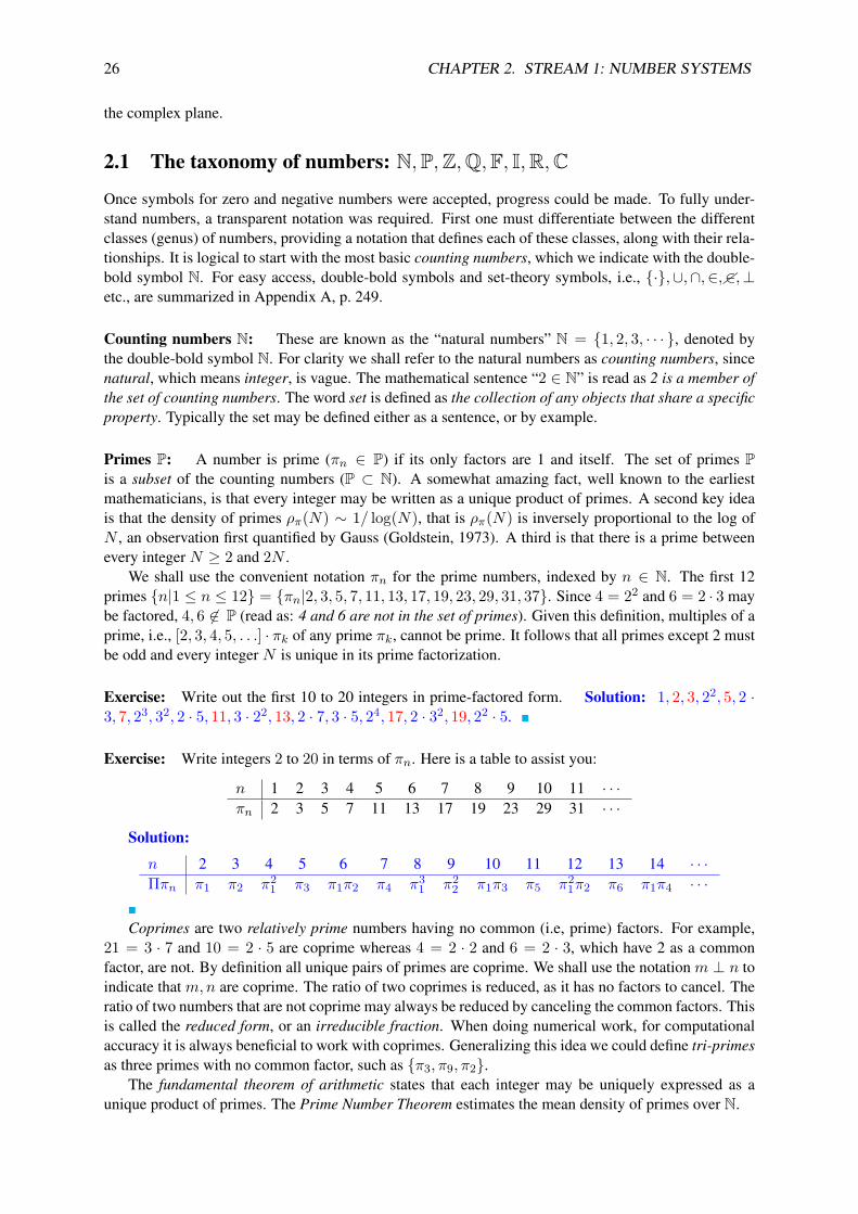
Exercise: Write out the first 10 to 20 integers in prime-factored form. Solution: 1, 2, 3, 22, 5, 2 ·3, 7, 23, 32, 2 · 5, 11, 3 · 22, 13, 2 · 7, 3 · 5, 24, 17, 2 · 32, 19, 22 · 5.
Exercise: Write integers 2 to 20 in terms of πn. Here is a table to assist you:
n 1 2 3 4 5 6 7 8 9 10 11 · · ·πn 2 3 5 7 11 13 17 19 23 29 31 · · ·
Solution:
n 2 3 4 5 6 7 8 9 10 11 12 13 14 · · ·Ππn π1 π2 π2
1 π3 π1π2 π4 π31 π2
2 π1π3 π5 π21π2 π6 π1π4 · · ·
Coprimes are two relatively prime numbers having no common (i.e, prime) factors. For example,21 = 3 · 7 and 10 = 2 · 5 are coprime whereas 4 = 2 · 2 and 6 = 2 · 3, which have 2 as a commonfactor, are not. By definition all unique pairs of primes are coprime. We shall use the notation m ⊥ n toindicate that m,n are coprime. The ratio of two coprimes is reduced, as it has no factors to cancel. Theratio of two numbers that are not coprime may always be reduced by canceling the common factors. Thisis called the reduced form, or an irreducible fraction. When doing numerical work, for computationalaccuracy it is always beneficial to work with coprimes. Generalizing this idea we could define tri-primesas three primes with no common factor, such as π3, π9, π2.
The fundamental theorem of arithmetic states that each integer may be uniquely expressed as aunique product of primes. The Prime Number Theorem estimates the mean density of primes over N.

2.1. THE TAXONOMY OF NUMBERS: P,N,Z,Q,F, I,R,C 27
Integers Z: These include positive and negative counting numbers and zero. Notionally we mightindicate this using set notation as Z = −N∪ 0 ∪N. Read this as The integers are in the set composedof the negative natural numbers −N, zero, and N.
Rational numbers Q: These are defined as numbers formed from the ratio of two integers. Given twonumbers n, d ∈ N, then n/d ∈ Q. Since d may be 1, it follows that the rationals include the countingnumbers as a subset. For example, the rational number 3/1 ∈ N.
The main utility of rational numbers is that that they can efficiently approximate any number on thereal line, to any precision. For example, the rational approximation π ≈ 22/7 has a relative error of≈0.04% (p. 54).
Fractional number F : A fractional number F is defined as the ratio of signed coprimes. If n, d ∈ ±P,then n/d ∈ F. Given this definition, F ⊂ Q = Z ∪ F. Because of the powerful approximating powerof rational numbers, the fractional set F has special utility. For example, π ≈ 22/7, 1/π ≈ 7/22 (to0.04%), e ≈ 19/7 to 0.15%, and
√2 ≈ 7/5 to 1%.
Irrational numbers I: Every real number that is not rational is irrational (Q ⊥ I). Irrational numbersinclude π, e and the square roots of primes. These are decimal numbers that never repeat, thus requiringinfinite precision in their representation. Such numbers cannot be represented on a computer, as theywould require an infinite number of bits (precision).
The rationals Q and irrationals I split the reals (R = Q∪ I, Q ⊥ I), thus each is a subset of the reals(Q ⊂ R, I ⊂ R). This relation is analogous to that of the integers Z and fractionals F, which split therationals (Q = Z ∪ F, Z ⊥ F) (thus each is a subset of the rationals (Z ⊂ Q, F ⊂ Q)).
Irrational numbers (I) were famously problematic for the Pythagoreans, who incorrectly theorizedthat all numbers were rational. Like∞, irrational numbers required mastering a new and difficult con-cept before they could even be defined: It was essential to understand the factorization of countingnumbers into primes (i.e., the fundamental theorem of arithmetic) before the concept of irrationals couldbe sorted out. Irrational numbers could only be understood once limits were mastered.
As discussed on p. 53, fractionals can approximate any irrational number with arbitrary accuracy.Integers are also important, but for a very different reason. All numerical computing today is done withQ = F∪Z. Indexing uses integers Z, while the rest of computing (flow dynamics, differential equations,etc.) is done with fractionals F (i.e., IEEE-754). Computer scientists are trained on these topics, andcomputer engineers need to be at least conversant with them.
Real numbers R: Reals are the union of rational and irrational numbers, namely R = Q ∪ I =Z ∪ F ∪ I. Lengths in Euclidean geometry are reals. Many people assume that IEEE 754 floating pointnumbers (c1985) are real (i.e., ∈ R). In fact they are rational (Q = F ∪ Z) approximations to realnumbers, designed to have a very large dynamic range. The hallmark of fractional numbers (F) is theirpower in making highly accurate approximations of any real number.
Using Euclid’s compass and ruler methods, one can make line length proportionally shorter orlonger, or (approximately) the same. A line may be made be twice as long, or an angle can be bi-sected. However, the concept of an integer length in Euclid’s geometry was not defined.4 Nor can oneconstruct an imaginary or complex line, as all lines are assumed to be real lengths. The development ofanalytic geometry was an analytic extension of Euclid’s simple (but important) geometrical methods.
Real numbers were first fully accepted only after set theory was developed by Cantor (1874) (Still-well, 2010, pp. 461). At first blush, this seems amazing, given how widely accepted real numbers aretoday. In some sense they were accepted by the Greeks, as lengths of real lines.
4As best I know.

28 CHAPTER 2. STREAM 1: NUMBER SYSTEMS
Complex numbers C: Complex numbers are best defined as ordered pairs of real numbers.5 Forexample, if a, b ∈ R and = −ı = ±
√−1, then c = a + b ∈ C. The word “complex,” as used here,
does not mean that the numbers are complicated or difficult. They are also known as “imaginary” num-bers, but this does not mean the numbers disappear. Complex numbers are quite special in engineeringmathematics, as roots of polynomials. The most obvious example is the quadratic formula, for the rootsof polynomials of degree 2, having coefficients ∈ C. All real numbers have a natural order on the realline. Complex numbers do not have a natural order. For example, > 1 makes no sense.
Today the common way to write a complex number is using the notation z = a + b ∈ C, wherea, b ∈ R. Here 1 =
√−1. We also define 1ı = −1 to account for the two possible signs of the square
root. Accordingly 12 = 1ı2 = −1.Cartesian multiplication of complex numbers follows the basic rules of real algebra, for example,
the rules of multiplying two monomials and polynomials. Multiplication of two first-degree polynomials(i.e., monomials) gives
(a+ bx)(c+ dx) = ac+ (ad+ bc)x+ bdx2.
If we substitute 1 for x, and use the definition 12 = −1, we obtain the Cartesian product of the twocomplex numbers
(a+ b)(c+ d) = ac− bd+ (ad+ bc).
Thus multiplication and division of complex numbers obey the usual rules of algebra.However, there is a critical extension: Cartesian multiplication only holds when the angles sum to
less than ±π, namely the range of the complex plane. When the angles add to more that ±π, one mustuse polar coordinates, where the angles add for angles beyond±π (Boas, 1987, p. 8). This is particularlystriking for the LT transform of a delay (Table C.3, p. 272).
Complex numbers can be challenging, providing unexpected results. For example, it is not obviousthat√
3 + 4 = ±(2 + ).
Exercise: Verify that√
3 + 4 = ±(2 + ). Solution: Square the left side gives√
3 + 42 = 3 + 4.Squaring the right side gives (2 + )2 = 4− 2 + 4 = 3 + 4. Thus the two are equal.
Exercise: What is special about this example? Solution: Note this is a 3,4,5 triangle. Can you findanother example like this one? Namely how does one find integers that obey Eq. 1.1 (p. 15)?
An alternative to Cartesian multiplication of complex numbers is to work in polar coordinates. Thepolar form of complex number z = a+ b is written in terms of its magnitude ρ =
√a2 + b2 and angle
θ = ∠z = tan−1 z = arctan z, as
z = ρeθ = ρ(cos θ + sin θ).
From the definition of the complex natural log function
ln z = ln ρeθ = ln ρ+ θ,
which is important, even critical, in engineering calculations. When the angles of two complex numbersare greater that ±π, one must use polar coordinates. It follows that when computing the phase, this ismuch different than the single- and double-argument ∠θ = arctan(z) function.
The polar representation makes clear the utility of a complex number: Its magnitude scales whileits angle Θ rotates. The property of scaling and rotating is what makes complex numbers useful inengineering calculations. This is especially obvious when dealing with impedances, which have complexroots with very special properties, as discussed on p. 156.
5A polynomial a+ bx and a 2-vector [a, b]T =[ab
]are also examples of ordered pairs.

2.1. THE TAXONOMY OF NUMBERS: P,N,Z,Q,F, I,R,C 29
Matrix representation: An alternative way to represent complex numbers is in terms of 2×2 matrices.This relationship is defined by the mapping from a complex number to a 2× 2 matrix
a+ b↔[a −bb a
], 1↔
[1 00 1
], 1↔
[0 −11 0
], eθ ↔
[cos(θ) − sin(θ)sin(θ) cos(θ)
]. (2.1)
The conjugate of a+ b is then defined as a− b↔[a b−b a
]. By taking the inverse of the 2× 2 matrix
(assuming |a + b| 6= 0), one can define the ratio of one complex number by another. Until you try outthis representation, it may not seem obvious, or even that it could work.
This representation proves that 1 is not necessary when defining a complex number. What 1 cando is to conceptually simplify the algebra. It is worth your time to become familiar with the matrixrepresentation, to clarify any possible confusions you might have about multiplication and division ofcomplex numbers. This matrix representation can save you time, heartache and messy algebra. Onceyou have learned how to multiply two matrices, it’s a lot simpler than doing the complex algebra. Inmany cases we will leave the results of our analysis in matrix form, to avoid the algebra altogether.6
Thus both representations are important. More on this topic may be found on p. 25.
History of complex numbers: It is notable how long it took for complex numbers to be accepted(1851), relative to when they were first introduced by Bombelli (16th century CE). One might havethought that the solution of the quadratic, known to the Chinese, would have settled this question. Itseems that complex integers (aka, Gaussian integers) were accepted before non-integral complex num-bers. Perhaps this was because real numbers (R) were not accepted (i.e., proved to exist, thus mathemat-ically defined) until the development of real analysis in the late 19th century, thus sorting out a properdefinition of the real number (due to the existence of irrational numbers).
Exercise: Using Matlab/Octave, verify that
a+ b
c+ d= ac+ bd+ (bc− ad)
c2 + d2 ←→[a −bb a
] [c −dd c
]−1
=[a −bb a
] [c d−d c
]1
c2 + d2 . (2.2)
Solution: The typical way may be using numerical examples. A better solution is to use a symboliccode:syms a b c d A BA=[a -b;b a];B=[c -d;d c];C=A*inv(B)
2.1.1 Numerical taxonomy:
A simplified taxonomy of numbers is given by the mathematical sentence
πk ∈ P ⊂ N ⊂ Z ⊂ Q ⊂ R ⊂ C.
This sentence says:
1. Every prime number πk is in the set of primes P,
2. which is a subset of the set of counting numbers N,
3. which is a subset of the set of integers Z = −N, 0,N,
6Sometimes we let the computer do the final algebra, numerically, as 2× 2 matrix multiplications.

30 CHAPTER 2. STREAM 1: NUMBER SYSTEMS
4. which is a subset of the set of rationals Q (ratios of signed counting numbers ±N),
5. which is a subset of the set of reals R,
6. which is a subset of the set of complex numbers C.
The rationals Q may be further decomposed into the fractionals F and the integers Z (Q = F ∪ Z), andthe reals R into the rationals Q and the irrationals I (R = I ∪ Q). This classification nicely defines allthe numbers (scalars) used in engineering and physics.
The taxonomy structure may be summarize with the single compact sentence, starting with the primenumbers πk and ending with complex numbers C:
πk ∈ P ⊂ N ⊂ Z ⊂ (Z ∪ F = Q) ⊂ (Q ∪ I = R) ⊂ C.
As discussed in Appendix A (p. 249), all numbers may be viewed as complex. Namely, every realnumber is complex if we take the imaginary part to be zero (Boas, 1987). For example, 2 ∈ P ⊂ C.Likewise every purely imaginary number (e.g., 0 + 1) is complex with zero real part.
Finally, note that complex numbers C, much like vectors, do not have “rank-order,” meaning onecomplex number cannot be larger or smaller than another. It makes no sense to say that > 1 or = 1(Boas, 1987). The real and imaginary parts, and the magnitude and phase, have order. Order seemsrestricted to R. If time t were complex, there could be no yesterday and tomorrow.7
2.1.2 Applications of integers
The most relevant question at this point is “Why are integers important?” First, we count with them, sowe can keep track of “how much.” But there is much more to numbers than counting: We use integersfor any application where absolute accuracy is essential, such as banking transactions (making change),the precise computing of dates (Stillwell, 2010, p. 70) and locations (“I’ll meet you at 34th and Vine atnoon on Jan. 1, 2034.”), or building roads or buildings out of bricks (objects built from a unit size).
To navigate we need to know how to predict the tides, the location of the moon and sun, etc. Integersare important, precisely because they are precise: Once a month there is a full moon, easily recognizable.The next day it’s slightly less than full. If one could represent our position as integers in time and space,we would know exactly where we are at all times. But such an integral representation of our position ortime is not possible.
The Pythagoreans claimed that all was integer. From a practical point of view, it seems they wereright. Today all computers compute floating point numbers as fractionals. However, in theory they werewrong. The error (difference) is a matter of precision.
Numerical Representations of I,R,C: When doing numerical work, one must consider how we maycompute within the set of reals (i.e., which contain irrationals). There can be no irrational numberrepresentation on a computer. The international standard of computation, IEEE floating point numbers,8
is based on rational approximation. The mantissa and the exponent are both integers, having sign andmagnitude. The size of each integer depends on the precision of the number being represented. AnIEEE floating-point number is rational because it has a binary (integer) mantissa, multiplied by 2 raisedto the power of a binary (integer) exponent. For example, π ≈ ±a2±b with a, b ∈ Z. In summary, IEEEfloating-point rational numbers cannot be irrational, because irrational representations would require aninfinite number of bits.
True floating point numbers contain irrational numbers, which must be approximated by fractionalnumbers. This leads to the concept of fractional representation, which requires the definition of themantissa, base and exponent, where both the mantissa and the exponent are signed. Numerical results
7One can usefully define ξ = x + 1j ct to be complex (x, t ∈ R), with x in meters [m], t is in seconds [s], and the speedof light co [m/s].
8IEEE 754: http://www.h-schmidt.net/FloatConverter/IEEE754.html.
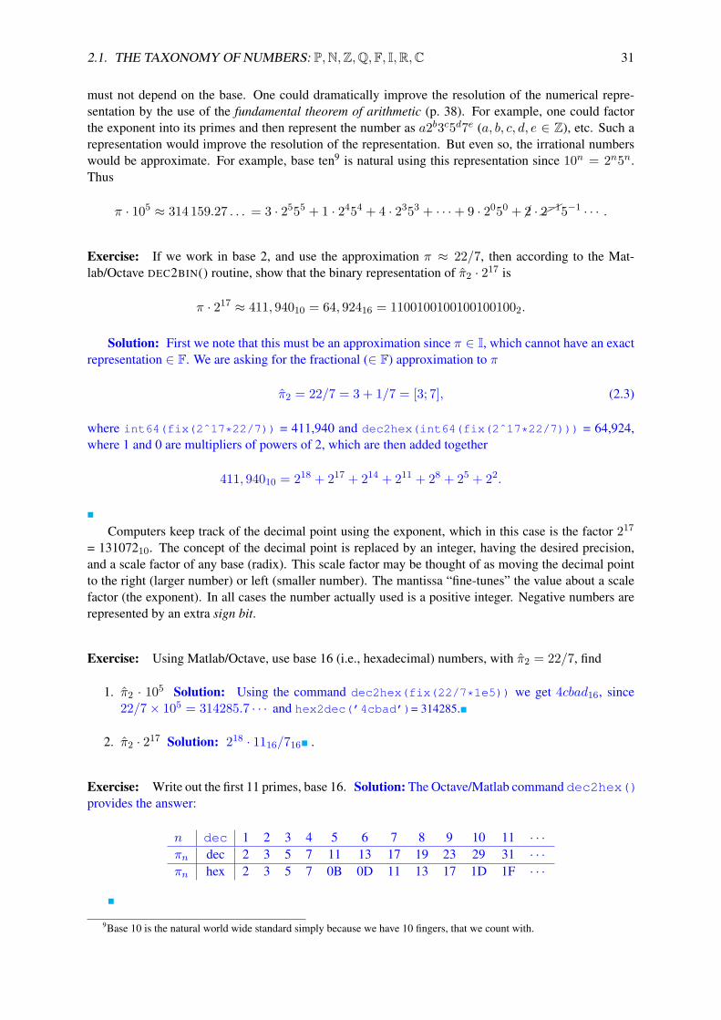
2.1. THE TAXONOMY OF NUMBERS: P,N,Z,Q,F, I,R,C 31
must not depend on the base. One could dramatically improve the resolution of the numerical repre-sentation by the use of the fundamental theorem of arithmetic (p. 38). For example, one could factorthe exponent into its primes and then represent the number as a2b3c5d7e (a, b, c, d, e ∈ Z), etc. Such arepresentation would improve the resolution of the representation. But even so, the irrational numberswould be approximate. For example, base ten9 is natural using this representation since 10n = 2n5n.Thus
π · 105 ≈ 314 159.27 . . . = 3 · 2555 + 1 · 2454 + 4 · 2353 + · · ·+ 9 · 2050 + 2 ·2−15−1 · · · .
Exercise: If we work in base 2, and use the approximation π ≈ 22/7, then according to the Mat-lab/Octave DEC2BIN() routine, show that the binary representation of π2 · 217 is
π · 217 ≈ 411, 94010 = 64, 92416 = 11001001001001001002.
Solution: First we note that this must be an approximation since π ∈ I, which cannot have an exactrepresentation ∈ F. We are asking for the fractional (∈ F) approximation to π
π2 = 22/7 = 3 + 1/7 = [3; 7], (2.3)
where int64(fix(2ˆ17*22/7)) = 411,940 and dec2hex(int64(fix(2ˆ17*22/7))) = 64,924,where 1 and 0 are multipliers of powers of 2, which are then added together
411, 94010 = 218 + 217 + 214 + 211 + 28 + 25 + 22.
Computers keep track of the decimal point using the exponent, which in this case is the factor 217
= 13107210. The concept of the decimal point is replaced by an integer, having the desired precision,and a scale factor of any base (radix). This scale factor may be thought of as moving the decimal pointto the right (larger number) or left (smaller number). The mantissa “fine-tunes” the value about a scalefactor (the exponent). In all cases the number actually used is a positive integer. Negative numbers arerepresented by an extra sign bit.
Exercise: Using Matlab/Octave, use base 16 (i.e., hexadecimal) numbers, with π2 = 22/7, find
1. π2 · 105 Solution: Using the command dec2hex(fix(22/7*1e5)) we get 4cbad16, since22/7× 105 = 314285.7 · · · and hex2dec(’4cbad’)= 314285.
2. π2 · 217 Solution: 218 · 1116/716 .
Exercise: Write out the first 11 primes, base 16. Solution: The Octave/Matlab command dec2hex()provides the answer:
n dec 1 2 3 4 5 6 7 8 9 10 11 · · ·πn dec 2 3 5 7 11 13 17 19 23 29 31 · · ·πn hex 2 3 5 7 0B 0D 11 13 17 1D 1F · · ·
9Base 10 is the natural world wide standard simply because we have 10 fingers, that we count with.

32 CHAPTER 2. STREAM 1: NUMBER SYSTEMS
Example: x = 217 × 22/7, using IEEE-754 double precision,10
x = 411, 940.562510
= 254 × 1198372= 0, 10010, 00, 110010, 010010, 010010, 0100102
= 0x48c9249216.
The exponent is 218 and the mantissa is 4, 793, 49010. Here the commas in the binary (0,1) string are tohelp visualize the quasi-periodic nature of the bit-stream. The numbers are stored in a 32 bit format, with1 bit for sign, 8 bits for the exponent and 23 bits for the mantissa. Perhaps a more instructive number is
x = 4, 793, 490.0= 0, 100, 1010, 100, 100, 100, 100, 100, 100, 100, 1002
= 0x4a92492416,
which has a repeating binary bit pattern of ((100))3, broken by the scale factor 0x4a. Even moresymmetrical is
x = 0x24, 924, 92416
= 00, 100, 100, 100, 100, 100, 100, 100, 100, 100, 1002
= 6.344, 131, 191, 146, 900× 10−17.
In this example the repeating pattern is clear in the hex representation as a repeating ((942))3, as rep-resented by the double brackets, with the subscript indicating the period, in this case, three digits. Asbefore, the commas are to help with readability and have no other meaning.
The representation of numbers is not unique. For example, irrational complex numbers have approx-imate rational representations (i.e., π ≈ 22/7). A better example is complex numbers z ∈ C, whichhave many representations, as a pair of reals (i.e., z = (x, y)), or by Euler’s formula, and matrices(θ ∈ R)
eθ = cos θ + j sin θ ↔[cos θ − sin θsin θ cos θ
].
At a higher level, differentiable functions, aka, analytic functions, may be represented by a single-valuedTaylor series expansion (p. 85), limited by its region of convergence (RoC).
Pythagoreans and Integers: The integer is the cornerstone of the Pythagorean doctrine, so much sothat it caused a fracture within the Pythagoreans when it was discovered that not all numbers are rational.One famous proof of such irrational numbers comes from the spiral of Theodorus, as shown in Fig. 2.1,where the short radius of each triangle has length bn =
√n with n ∈ N, and the long radius (the
hypotenuses) is cn =√
1 + b2n =√
1 + n. This figure may be constructed using a compass and rulerby maintaining right triangles.
Public-key security: An important application of prime numbers is public-key encryption, essentialfor internet security applications (e.g., online banking). Most people assume encryption is done by apersonal login and passwords. Passwords are fundamentally insecure, for many reasons. Decryptiondepends on factoring large integers, formed from products of primes having thousands of bits.11 Thesecurity is based on the relative ease of multiplying large primes, along with the virtual impossibility offactoring their products.
10http://www.h-schmidt.net/FloatConverter/IEEE754.html11It would seem that public-key encryption could work by having two numbers with a common prime, and then using the
Euclidean algorithm, the greatest common divisor (GCD) could be worked out. One of the integers could be the public-keyand the second could be the private key.

2.1. THE TAXONOMY OF NUMBERS: P,N,Z,Q,F, I,R,C 33
3
2
4
5
6
7
8
9
17
16
15
14
1312
1110
1
1
1
1
Figure 2.1: This construction is called the spiral of Theodorus, made from contiguous triangles having lengths a = 1,bn =
√n, with n ∈ N, and cn =
√n+ 1. In this way, each value of c2
n = b2n + 1 ∈ N. Note that none of these right-triangles
are Pythagorean triplets. (Adapted from https://en.wikipedia.org/wiki/sprial of Theodorus).
When a computation is easy in one direction, but its inverse is impossible, it is called a trap-doorfunction. We shall explore trapdoor functions in Appendix 2. If everyone were to switch from passwordsto public-key encryption, the internet would be much more secure.12
Puzzles: Another application of integers is imaginative problems that use integers. An example is theclassic Chinese four stone problem: Find the weight of four stones that can be used with a scale toweigh anything (e.g., salt, gold) between 0, 1, 2, . . . , 40 [gm] (Fig. 11.1, p. 118 in Assignment AE-2).As with the other problems, the answer is not as interesting as the method, since the problem may beeasily recast into a related one. This type of problem can be found in airline magazines as amusementon a long flight. This puzzle is best cast as a linear algebra problem, with integer solutions. Again, onceyou know the trick, it is “easy.”13
12https://fas.org/irp/agency/dod/jason/cyber.pdf13Whenever someone tells you something is “easy,” you should immediately appreciate that it is very hard, but once you
learn a concept, the difficulty evaporates.

34 CHAPTER 2. STREAM 1: NUMBER SYSTEMS
2.2 Exercises NS-1
Topic of this homework:
Introduction to MATLAB/OCTAVE (see the Matlab or Octave tutorial for help).Deliverable: Report with charts and answers to questions. Hint: Use LATEX.14
Plotting complex quantities in Octave/Matlab
Problem # 1: Consider the functions f(s) = s2 + 6s+ 25 and g(s) = s2 + 6s+ 5.
–Q 1.1Find the zeros of functions f(s) and g(s) using the command roots().
–Q 1.2: Show the roots of f(s) as red circles and of g(s) as blue plus signs.The x-axis should display the real part of each root, and the y-axis should display the imaginary part.Use hold on and grid on when plotting the roots.
–Q 1.3 Give your figure the title ‘Complex Roots of f(s) and g(s)’ Label the x- and y-axis‘Real Part’ and ‘Imaginary Part.’Hint: use xlabel and ylabel. Type ylim([-10 10]) and xlim([-10 10]), to expand theaxes.
Problem # 2: Consider the function h(t) = ej2πft for f = 5 and t=[0:0.01:2].
–Q 2.1: Use subplot to show the real and imaginary parts of h(t)Make two graphs in one figure. Label the x-axes ‘Time (s)’ and the y-axes ‘Real Part’ and ‘ImaginaryPart’.
–Q 2.2: Use subplot to plot the magnitude and phase parts of h(t).Use the command angle or unwrap(angle()) to plot the phase. Label the x-axes ‘Time (s)’ andthe y-axes ‘Magnitude’ and ‘Phase (radians)’.
Prime numbers, infinity, etc. in Octave/Matlab
Problem # 3: Prime numbers, infinity, etc.
–Q 3.1: Use the Matlab function factor to find the prime factors of 123, 248, 1767, and999,999.
–Q 3.2: Use the Matlab function isprime to check if 2, 3 and 4 are prime numbers.What does the function isprime return when a number is prime, or not prime? Why?
14http://www.overleaf.com

2.2. EXERCISES NS-1 35
–Q 3.3: Use the Matlab/Octave function primes.m to generate prime numbers between1 and 106
Save them in a vector x. Plot this result using the command hist(x).
–Q 3.4: Now try [n,bincenters] = hist(x).Use length(n) to find the number of bins.
–Q 3.5: Set the number of bins to 100 by using an extra input argument to the functionhist.Show the resulting figure and give it a title and axes labels.
Problem # 4: Inf, NaN and logarithms in Octave/Matlab
–Q 4.1: Try 1/0 and 0/0 in the Octave/Matlab command window.What are the results? What do these ‘numbers’ mean in Matlab?
–Q 4.2: Try log(0) in the command window.In Matlab, the natural logarithm ln(·) is computed using the function log (log10, and log2 are computedusing log10 and log2).
–Q 4.3: Try log(-1) in the command window. Do you get what you expect for ln(−1)?Show how Matlab arrives at the answer by considering −1 = eiπ.
–Q 4.4: Try log(exp(j*sqrt(pi))) (i.e., log e√π) in the command window. What
do you expect? Show how Octave/Matlab arrives at the answer by considering −1 = eiπ.
–Q 4.5: What does inverse mean in this context? What is the inverse of ln f(x)?
–Q 4.6: What is a decibel? (Look up decibels on the internet.)
Problem # 5: Very large primes on Intel computers
–Q 5.1: Find the largest prime number that can be stored on an Intel 64 bit computer, whichwe call πmax.Hint: As explained in the Matlab/Octave command help flintmax, the largest positive integer is253, however the largest integer that can be factored is 232 =
√264. Explain the logic of your answer.
Hint: help isprime().
Problem # 6: Suppose you are interested in primes that are greater than πmax. How can youfind them on an Intel computer (i.e., one using IEEE-floating point)?
–Q 6.1: Thus consider a sieve containing only odd numbers, starting from 3 (not 2).Hint 1: Since every prime number greater than 2 is odd, there is no reason to check the even numbers.nodd ∈ N/2 contain all the primes other than 2.
Problem # 7: The following idenity is interesting:

36 CHAPTER 2. STREAM 1: NUMBER SYSTEMS
1 = 12
1 + 3 = 22
1 + 3 + 5 = 32
1 + 3 + 5 + 7 = 42
1 + 3 + 5 + 7 + 9 = 52
· · ·N−1∑n=0
2n+ 1 = N2.
–Q 7.1: Can you find a proof?15
15This problem came from an exam problem for Math 213, Fall 2016.

2.3. THE ROLE OF PHYSICS IN MATHEMATICS 37
2.3 The role of physics in mathematics
Bells, chimes and eigenmodes: Integers naturally arose in art, music and science. Examples includethe relations between musical notes, the natural eigenmodes (tones) of strings and other musical instru-ments. These relations were so common that Pythagoras believed that to explain the physical world (aka,the universe), one needed to understand integers. As discussed on p. 13, “all is integer” was a seductivesong.
As will be discussed on p. 69, it is best to view the relationship between acoustics, music and math-ematics as historical, since these topics inspired the development of mathematics. Today integers play akey role in quantum mechanics, again based on eigenmodes, but in this case, eigenmodes follow fromsolutions of Schrodinger equation, with the roots of the characteristic equation being purely imaginary.If there were a real part (i.e., damping), the modes would not be integers.
As discussed by Salmon (1946, p. 201), Schrodinger’s equation follows directly from the Websterhorn equation. While Morse (1948, p. 281) (a student of Arnold Sommerfeld) fails to make the directlink, he comes close to the same view when he shows that the real part of the horn resistance goes exactlyto zero below a cutoff frequency. He also discusses the trapped modes inside musical instruments dueto the horn flair (p. 268). One may assume Morse read Salmon’s paper on horns, since he cites Salmon(Morse, 1948, Footnote 1, p. 271).
Engineers are so accustomed to working with real (or complex) numbers, the distinction betweenreal (i.e., irrational) and fractional numbers is rarely acknowledged. Integers, on the other-hand, arisein many contexts. One cannot master programming computers without understanding integer, hexadec-imal, octal, and binary representations, since all numbers in a computer are represented in numericalcomputations in terms of rationals (Q = Z ∪ F).16
As discussed on p. 26, the primary reason integers are so important is their absolute precision.Every integer n ∈ Z is unique,17 and has the indexing property, which is essential for making lists thatare ordered, so that one can quickly look things up. The alphabet also has this property (e.g., a book’sindex).
Because of the integer’s absolute precision, the digital computer quickly overtook the analog com-puter, once it was practical to make logic circuits that were fast. From 1946 the first digital computerwas thought to be the University of Pennsylvania’s Eniac. We now know that the code-breaking effortin Bletchley Park, England, under the guidance of Alan Turing, created the first digital computer (TheColossus), used to break the WWII German “Enigma” code. Due to the high secrecy of this war effort,the credit was only acknowledged in the 1970s when the project was finally declassified.
There is zero possibility of analog computing displacing digital computing, due to the importanceof precision (and speed). But even with binary representation, there is a non-zero probability of error,for example on a hard drive, due to physical noise. To deal with this, error correcting codes have beendeveloped, reducing the error by many orders of magnitude. Today error correction is a science, andbillions of dollars are invested to increase the density of bits per area, to increasingly larger factors. Afew years ago the terabyte drive was unheard of; today it is standard. In a few years petabyte drives willcertainly become available. It is hard to comprehend how these will be used by individuals, but they areessential for on-line (cloud) computing.
2.3.1 The role of mathematics in physics: The three streams
Modern mathematics is built on a hierarchical construct of fundamental theorems, as summarized inthe boxed material (p. 38). The importance of such theorems cannot be overemphasized. Gauss’s andStokes’s laws play a major role in understanding and manipulating Maxwell’s equations. Every engi-neering student needs to fully appreciate the significance of these key theorems. If necessary, memorizethem. But that will not do over the long run, as each and every theorem must be fully understood. For-
16See Appendix A (p. 249) for a review of mathematical notation.17Check out the history of 1729 = 13 + 123 = 93 + 103.

38 CHAPTER 2. STREAM 1: NUMBER SYSTEMS
tunately most students already know several of these theorems, but perhaps not by name. In such cases,it is a matter of mastering the vocabulary.
The three streams of mathematics:1. Number systems: Stream 1
• arithmetic
• prime number
2. Geometry: Stream 2
• algebra
3. Calculus: Stream 3 (Flanders, 1973)
• Leibniz R1
• complex C ⊂ R2
• vectors R3,Rn,R∞
– Gauss’s law (divergence theorem)– Stokes’s law (curl theorem, or Green’s theorem)– Vector calculus (Helmholtz’s theorem)
These theorems are naturally organized, and may be thought of, in terms of Stillwell’s three streams.For Stream 1 there is the fundamental theorem of arithmetic and the prime number theorem. ForStream 2 there is the fundamental theorem of algebra while for Stream 3 there are a host of theoremson calculus, ordered by their dimensionality. Some of these theorems seem trivial (e.g., the fundamentaltheorem of arithmetic). Others are more challenging, such as the fundamental theorem of vector calculusand Green’s theorem.
Complexity should not be confused with importance. Each of these theorems, as stated, is funda-mental. Taken as a whole, they are a powerful way of summarizing mathematics.
2.3.2 Stream 1: Prime number theorems
There are two easily described fundamental theorems about primes:
1. The fundamental theorem of arithmetic: This states that every integer n ∈ Z may be uniquelyfactored into prime numbers. This raises the question of the meaning of factor (split into aproduct). The product of two integers m,n ∈ Z is mn =
∑m n =
∑nm. For example,
2 ∗ 3 = 2 + 2 + 2 = 3 + 3.
2. The prime number theorem: One would like to know how many primes there are. That is easy:|P| = ∞ (the size of the set of primes is infinite). A better way of asking this questions is Whatis the average density of primes, in the limit as n → ∞? This question was answered, for allpractical purposes, by Gauss, who in his free time computed the first three million primes byhand. He discovered that, to a good approximation, the primes are equally likely on a log scale.This is nicely summarized by the limerick:
Chebyshev said, and I say it again: There is always a prime between n and 2n.
attributed to the mathematician Pafnuty Chebyshev, which nicely summarizes theorem 3 (Still-well, 2010, p. 585).
When the ratio of two frequencies (pitches) is 2, the relationship is called an octave. With a slight stretchof terminology, we could say there is at least one prime per octave.
In modern western music the octave is further divided into 12 ratios called semitones equal to 12√2.Twelve semitones is an octave. In the end, it is a question of the density of primes on a log-log (i.e.,

2.3. THE ROLE OF PHYSICS IN MATHEMATICS 39
ratio) scale. One might wonder about the maximum number of primes per octave, as a function of N , orask for the fractions of an octave in the neighborhood of each prime.
2.3.3 Stream 2: Fundamental theorem of algebra
This theorem states that every polynomial in x of degree N
PN (x) =N∑k=0
akxk (2.1)
has at least one root (p. 99). When a common root is factored out, the degree of the polynomial is reducedby 1. Applied recursively, a polynomial of degreeN hasN roots. Note there areN+1 coefficients (i.e.,[aN , aN−1, · · · , a0]). If we are only interested in the roots of PN (x) it is best to define aN = 1, whichdefines the monic polynomial. If the roots are fractional numbers this might be possible. However if theroots are irrational numbers (likely), a perfect factorization is at least unlikely if not impossible.
2.3.4 Stream 3: Fundamental theorems of calculus
In Sections 5.8 and 5.8.6 we will deal with each of the theorems for Stream 3, where we consider theseveral fundamental theorems of integration, starting with Leibniz’s formula for integration on the realline (R), then progressing to complex integration in the complex plane (C) (Cauchy’s theorem), which isrequired for computing the inverse Laplace transform. Gauss’s and Stokes’s laws for R2 require closedand open surfaces, respectively. One cannot manipulate Maxwell’s equations, fluid flow, or acoustics,without understanding these theorems. Any problem that deals with the wave equation in more thanone dimension requires an understanding of these theorems. They are the basis of the derivation of theKirchhoff voltage and current laws.
Finally we define the four basic vector operations based on the gradient operator differential vectoroperator, which have been given mnemonic abbreviations (see p. 225),
∇ ≡ x ∂
∂x+ y ∂
∂y+ z ∂
∂z, (2.2)
pronounced as “del” (preferred) or “nabla,” which are the gradient ∇(), divergence∇·(), curl ∇×().Second order operators such as the scalar Laplacian ∇·∇() = ∇2() may be constructed from first
order operators. The most important of these is the vector Laplacian ∇2() which is required whenworking with Maxwell’s Wave Equations.
The first three operations are defined in terms of integral operations on a surface in 1, 2 or 3 di-mensions, by taking the limit as that surface, or the volume contained within, goes to zero. These threedifferential operators are essential to fully understand Maxwell’s equations, the crown jewel of mathe-matical physics. Hence mathematics plays a key role in physics, as does physics in math.
2.3.5 Other key mathematical theorems
Besides the widely recognized fundamental theorems for the three streams, there are a number of equallyimportant theorems that have not yet been labeled as “fundamental.”18
The widely recognized Cauchy integral theorem is an excellent example, since it is a stepping stoneto Green’s theorem and the fundamental theorem of complex calculus. In Sections 4.5 (p. 167) we clarifythe contributions of each of these special theorems.
Once these fundamental theorems of integration (Stream 3) have been mastered, the student is readyfor the complex frequency domain, which takes us back to Stream 2 and the complex frequency plane(s = σ+ω ∈ C). While the Fourier and LT ’s are taught in mathematics courses, the concept of complexfrequency is rarely mentioned. The complex frequency domain (p. 131) and causality are fundamentally
18It is not clear what it takes to reach this more official sounding category.

40 CHAPTER 2. STREAM 1: NUMBER SYSTEMS
related (pp. 178–179), and are critical for the analysis of signals and systems, and especially whendealing with the concept of impedance (p. 156).
Without the concept of time and frequency, one cannot develop an intuition for the Fourier andLaplace transforms, especially within the context of engineering and mathematical physics. The Fouriertransform covers signals, while the Laplace transform describes systems. Separating these two concepts,based on their representations as Fourier and Laplace transforms, is an important starting place forunderstanding physics and the role of mathematics. However, these methods, by themselves, do notprovide the insight into physical systems necessary to be productive, or better, creative with these tools.One needs to master the tools of differential equations, and then partial differential equations, to fullyappreciate the world that they describe. Electrical and mechanical networks, composed of inductors,capacitors and resistors, are isomorphic to mechanical systems composed of masses, springs and dash-pots. Newton’s laws are analogous to those of Kirchhoff, which are the rules needed to analyze simplephysical systems composed of linear (and nonlinear) sub-components. When lumped-element systemsare taken to the limit, in several dimensions, we obtain Maxwell’s partial differential equations, the lawsof continuum mechanics, and beyond.
The ultimate goal of this book is to make you aware of and productive in using these tools. Thismaterial can be best absorbed by treating it chronologically through history, so you can see how thisbody of knowledge came into existence, through the minds and hands of Galileo, Newton, Maxwell andEinstein. Perhaps one day you too can stand on the shoulders of the giants who went before you.
2.4 Applications of prime number
If someone asked you for a theory of counting numbers, I suspect you would laugh and start counting.It sounds like either a stupid question, or a bad joke. Yet integers are a rich topic, so the question is noteven slightly dumb. It is somewhat amazing that even birds and bees can count. While I doubt birdsand bees can recognize primes, cicadas and other insects only crawl out of the ground in prime numbercycles, (e.g., 13 or 17 year cycles). If you have ever witnessed such an event (I have), you will neverforget it. Somehow they know. Finally, there is an analytic function, first introduced by Euler, based onhis analysis of the sieve, now known as the Riemann zeta function ζ(s), which is complex analytic, withits poles at the logs of the prime numbers. The properties of this function are truly amazing, even fun.Many of the questions and answers about primes go back to at least the early Chinese (c1500 BCE).
The importance of prime numbers: Each prime perfectly predicts multiples of that prime, but thereseems to be no regularity in predicting primes. It follows that prime numbers are the key to the theoryof numbers, because of the fundamental theorem of arithmetic (FTA),
Likely the first insight into the counting numbers started with the sieve, shown in Fig. 2.2. A sieveanswers the question “How can one identify the prime numbers?” The answer comes from looking forirregular patterns in the counting numbers, by playing the counting numbers against themselves.
A recursive sieve method for finding primes was first devised by the Greek Eratosthenes (O’Neill,2009).
For example, starting from π1 = 2 one strikes out all even numbers 2 · (2, 3, 4, 5, 6, · · · ), but not 2.By definition the multiples are products of the target prime (2 in our example) and every another integer(n ≥ 2). In this way all the even numbers are removed in this first iteration. The next remaining integer(3 in our example) is identified as the second prime π2. Then all the multiples of π2 = 3 are removed.The next remaining number is π3 = 5, so all multiples of π3 = 5 are removed (i.e.,10,15,25 etc., · · · ).This process is repeated until all the numbers of the list have either been canceled or identified as prime.
As the word sieve implies, this process takes a heavy toll on the integers, rapidly pruning the non-primes. In four iterations of the sieve algorithm, all the primes below N = 50 are identified in red. Thefinal set of primes is displayed in step 4 of Fig. 2.2.
Once a prime greater than N/2 has been identified (25 in the example), the recursion stops, sincetwice that prime is greater than N , the maximum number under consideration. Thus once
√49 has
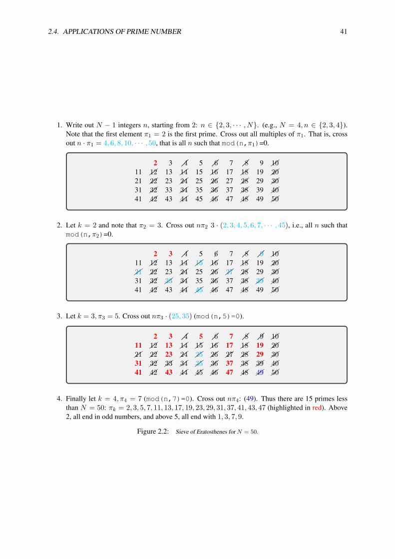
2.4. APPLICATIONS OF PRIME NUMBER 41
1. Write out N − 1 integers n, starting from 2: n ∈ 2, 3, · · · , N. (e.g., N = 4, n ∈ 2, 3, 4).Note that the first element π1 = 2 is the first prime. Cross out all multiples of π1. That is, crossout n · π1 = 4, 6, 8, 10, · · · , 50, that is all n such that mod(n,π1)=0.
2 3 4 5 6 7 8 9 1011 12 13 14 15 16 17 18 19 2021 22 23 24 25 26 27 28 29 3031 32 33 34 35 36 37 38 39 4041 42 43 44 45 46 47 48 49 50
2. Let k = 2 and note that π2 = 3. Cross out nπ2 3 · (2, 3, 4, 5, 6, 7, · · · , 45), i.e., all n such thatmod(n,π2)=0.
2 3 4 5 6 7 8 9 1011 12 13 14 15 16 17 18 19 2021 22 23 24 25 26 27 28 29 3031 32 33 34 35 36 37 38 39 4041 42 43 44 45 46 47 48 49 50
3. Let k = 3, π3 = 5. Cross out nπ3 · (25, 35) (mod(n,5)=0).
2 3 4 5 6 7 8 9 1011 12 13 14 15 16 17 18 19 2021 22 23 24 25 26 27 28 29 3031 32 33 34 35 36 37 38 39 4041 42 43 44 45 46 47 48 49 50
4. Finally let k = 4, π4 = 7 (mod(n,7)=0). Cross out nπ4: (49). Thus there are 15 primes lessthan N = 50: πk = 2, 3, 5, 7, 11, 13, 17, 19, 23, 29, 31, 37, 41, 43, 47 (highlighted in red). Above2, all end in odd numbers, and above 5, all end with 1, 3, 7, 9.
Figure 2.2: Sieve of Eratosthenes for N = 50.

42 CHAPTER 2. STREAM 1: NUMBER SYSTEMS
been reached, all the primes have been identified (this follows from the fact that the next prime πn ismultiplied by an integer n = 1, . . . N ).
When using a computer, memory efficiency and speed are the main considerations. There are variousschemes for making the sieve more efficient. For example, the recursion nπk = (n − 1)πk + πk willspeed up the process by replacing the multiply with an addition of πk.
Two fundamental theorems of primes: Early theories of numbers revealed two fundamental theo-rems (there are many more than two), as discussed on pages 37, 40 and 25). The first of these is thefundamental theorem of arithmetic, which says that every integer n ∈ N greater than 1 may be uniquelyfactored into a product of primes
n =KΠk=1
πβkk , (2.3)
where k = 1, . . . ,K indexes the integer’s K prime factors πk ∈ P. Typically prime factors appear morethan once, for example 25 = 52. To make the notation compact we define the multiplicity βk of eachprime factor πk. For example 2312 = 23 · 172 = π3
1 π27 (i.e., π1 = 2, β1 = 3;π7 = 17, β7 = 2) and
2313 = 32 · 257 = π23 π55 (i.e., π2 = 3, β3 = 2;π55 = 257, β55 = 1). Our demonstration of this is
empirical, using the Matlab/Octave factor(N) routine, which factors N .19
What seems amazing is the unique nature of this theorem. Each counting number is uniquely repre-sented as a product of primes. No two integers can share the same factorization. Once you multiply thefactors out, the result is unique (N ). Note that it’s easy to multiply integers (e.g., primes), but expensiveto factor them. And factoring the product of three primes is significantly more difficult than factoringtwo.
Factoring is much more expensive than division. This is not due to the higher cost of division overmultiplication, which is less than a factor of 2.20 Dividing the product of two primes, given one, is trivial,slightly more expensive that multiplying. Factoring the product of two primes is nearly impossible, asone needs to know what to divide by. Factoring means dividing by some integer and obtaining anotherinteger with remainder zero.
This brings us to the prime number theorem (PNT). The security problem is the reason why thesetwo theorems are so important: 1) Every integer has a unique representation as a product of primes, and2) the density of primes is large (see the discussions on p. 38). Thus security reduces to the “needle inthe haystack problem” due to the cost of a search.
Thus one could factor a product of primes N = πkπl by doing M divisions, where M is the numberof primes less than N . This assumes the list of primes less than N are known. However, most integersare not a simple product of two primes
But the utility of using prime factorization has to do with their density. If we were simply looking upa few numbers from a short list of primes, it would be easy to factor them. But given that their densityis logarithmic (1 per octave), factoring becomes at a very high computational cost.
2.4.1 Greatest common divisor (Euclidean algorithm)
The Euclidean algorithm is a systematic method to find the largest common integer factor k betweentwo integers n,m, denoted k = gcd(n,m), where n,m, k ∈ N (Graham et al., 1994). For example,15 = gcd(30, 105) since, when factored (30, 105) = (2 · 3 · 5, 7 · 3 · 5) = 3 · 5 · (2, 7) = 15 · (2, 7). TheEuclidean algorithm was known to the Chinese (i.e., not discovered by Euclid) (Stillwell, 2010, p. 41).Two integers are said to be coprime if their gcd is 1 (i.e., they have no common factor).
The Euclidean algorithm: The algorithm is best explained by a trivial example: Let the two numbersbe 6, 9. At each step the smaller number (6) is subtracted from the larger (9) and the smaller number
19If you wish to be a mathematician, you need to learn how to prove theorems. If you’re a physicist, you are happy thatsomeone else has already proved them, so that you can use the result.
20https://streamcomputing.eu/blog/2012-07-16/how-expensive-is-an-operation-on-a-cpu/

2.4. APPLICATIONS OF PRIME NUMBER 43
Examples of the GCD: l = gcd(m,n)• Examples (m,n, l ∈ Z):
– 5 = gcd(13 · 5, 11 · 5). The GCD is the common factor 5.
– gcd(13 · 10, 11 · 10) = 10 (gcd(130, 110) = 10 = 2 · 5, is not prime)
– gcd(1234, 1024) = 2 since 1234 = 2 · 617, 1024 = 210
– gcd(πkπm, πkπn) = πk– l = gcd(m,n) is the part that cancels in the fraction m/n ∈ F– m/gcd(m,n) ∈ Z
• Coprimes (m ⊥ n) are numbers with no distinct common factors: i.e., gcd(m,n)=1
– The GCD of two primes is always 1: gcd(13,11) = 1, gcd(πm, πn)=1 (m 6= n)
– m = 7 · 13, n = 5 · 19⇒ (7 · 13) ⊥ (5 · 19)– If m ⊥ n then gcd(m,n) = 1– If gcd(m,n) = 1 then m ⊥ n
• The GCD may be extended to polynomials: e.g., gcd(ax2 + bx+ c, αx2 + βx+ γ)
– gcd((x− 3)(x− 4), (x− 3)(x− 5))= (x− 3)– gcd(x2 − 7x+ 12, 3(x2 − 8x+ 15))= 3(x− 3)– gcd(x2 − 7x+ 12, (3x2 − 24x+ 45)= 3(x− 3)– gcd( (x− 2π)(x− 4), (x− 2π)(x− 5) )= (x− 2π) (Needs long division)
and the difference (the remainder) are saved. This process continues until the two resulting numbers areequal, which is the GCD. For our example: 9− 6 = 3, leaving the smaller number 6 and the difference3. Repeating this we get 6 − 3 = 3, leaving the smaller number 3 and the difference 3. Since thesetwo numbers are the same we are done, thus 3 = gcd(9, 6). We can verify this result by factoring [e.g.,(9, 6) = 3(3, 2)]. The value may also be numerically verified using the Matlab/Octave GCD commandgcd(6, 9), which returns 3.
mm-n
m-2nm-3n
m-6nm-7n
m-k
n
kn n
Figure 2.3: The Euclidean algorithm recursively subtracts n from m until the remainder m − kn is either less than n orzero. Note that this recursion is the same as mod(m,n). Thus the GCD recursively computes mod(m,n) until the remainderrem(m,n) is less than n, which is denoted the GCD’s turning-point. It then swaps m,n, so that n < m. This repeats, untilit terminates on the GCD. Due to its simplicity this is called the direct method for finding the GCD. For the case depicted herethe value of k, that renders the remainder m − 6n < n. If one more step were taken beyond the turning-point (k = 7), theremainder would become negative. Thus the turning-point satisfies the linear relation m− αn = 0 with α ∈ R.
Direct matrix method: The GCD may be written as a matrix recursion given the starting vector(m0, n0)T . The recursion is then [
mk+1nk+1
]=[1 −10 1
] [mk
nk
]. (2.4)

44 CHAPTER 2. STREAM 1: NUMBER SYSTEMS
This recursion continues until mk+1 < nk+1, at which point m and n must be swapped. The process isrepeated until mk = nk, which equals the GCD. We call this the direct method (see Fig. 2.3). The directmethod is inefficient because it recursively subtracts nk many times until the resulting mk is less thannk. It also must test for m ≤ n after each subtraction, and then swap them if mk < nk. If they are equalwe are done.
The GCD’s turning-point may be defined using the linear interpolation m − αn = 0, α ∈ R,where the solid line cross the abscissa in Fig. 2.3. If, for example, l = 6+43/97 ≈ 6.443298 · · · ,then 6 = bm/nc < n and α ∈ F ∈ R. This is nonlinear (truncation) arithmetic, which is a naturalproperty of the GCD. The floor() functions finds the turning-point, where we swap the twonumbers, since by definition, m > n. In this example 6 = blc.
Exercise: Show that [1 −10 1
]n=[1 −n0 1
]Solution: Let n = 2. Next show that the recursive multiplication add 1 to the upper right corner.
Why is the GCD important? The utility of the GCD algorithm arises directly from the fundamentaldifficulty in factoring large integers. Computing the GCD, using the Euclidean algorithm, is low cost,compared to factoring when finding the coprime factors, which is extremely expensive. The utilitysurfaces when the two numbers are composed of very large primes.
When two integers have no common factors they are said to be coprime and their GCD is 1. Theratio of two integers which are coprime is automatically in reduced form (they have no common factors).For example, 4/2 ∈ Q is not reduced since 2 = gcd(4, 2) (with a zero remainder). Canceling out thecommon factor 2 gives the reduced form 2/1 ∈ F. Thus if we wish to form the ratio of two integers,first compute the GCD, then remove it from the two numbers to form the ratio. This assures the rationalnumber is in its reduced form (∈ F rather than ∈ Q). If the GCD were 103 digits, it is obvious that anycommon factor would need to be be removed, thus greatly simplifying further computation. This willmake a huge difference when using IEEE-754.
The floor function and the GCD are related in an important way, as discussed next.
Indirect matrix method: A much more efficient method uses the floor() function, which is calleddivision with rounding, or simply the indirect method. Specifically the GCD may be written in one stepas [
mn
]k+1
=[0 11 −
⌊mn
⌋] [mn
]k
. (2.5)
This matrix is simply Eq. 2.4 to the power bm/nc, followed by swapping the inputs (the smaller mustalways be on the bottom).
The GCD and multiplication: Multiplication is simply recursive addition, and finding the GCD takesadvantage of this fact. For example 3 ∗ 2 = 3 + 3 = 2 + 2 + 2. Since division is the inverse ofmultiplication, it must be recursive subtraction.
The GCD and long division: When one learns how to divide a smaller number into a larger one, theymust learn how to use the GCD. For example, suppose we which to compute 6 ÷ 110. One starts byfinding out how many times 6 goes into 11. Since 6 × 2 = 12, which is larger than 11, the answeris 1. We then subtract 6 from 11 to find the remainder 5. This is, of course, the floor function (e.g.,b11/6c = 1, b11/5c = 2).

2.4. APPLICATIONS OF PRIME NUMBER 45
Example: Start with the two integers [873, 582]. In factored form these are [π25 · 32, π25 · 3 · 2]. Giventhe factors, we see that the largest common factor is π25 · 3 = 291 (π25 = 97). When we take the ratioof the two numbers this common factor cancels
873582 =
π25 · 3 · 3π25 · 3 · 2
= 32 = 1.5.
Of course if we divide 582 into 873 we will numerically obtain the answer 1.5 ∈ F.
Exercise: What does it mean to reach the turning-point when using the Euclidean algorithm? So-lution: When m/n − bm/nc < n we have reached a turning-point. When the remainder is zero (i.e.,m/n− bm/nc = 0), we have reached the GCD.
Exercise: Show that in Matlab/Octave rat(873/582) = 1 + 1/(−2) gives the wrong answer(rats(837/582)=3/2). Hint: Factor the two numbers and cancel out the gcd. Solution: Since
factor(873) = 3 · 3 · 97 and factor(582) = 2 · 3 · 97,
the gcd is 3*97, thus 3/2 = 1 + 1/2 is the correct answer. But due to rounding methods, it is not 3/2.As an example, in Matlab/Octave rat(3/2)=2+1/(-2). Matlab’s rat() command uses roundingrather than the floor function, which explains the difference. When the rat() function produces nega-tive numbers, rounding is employed.
Exercise: Divide 10 into 99, the floor function (floor(99/10)) must be used, followed by theremainder function (rem(99,10)). Solution: When we divide a smaller number into a larger one,we must first find the floor followed by the remainder. For example 99/10 = 9 + 9/10 has a floor of 9 anda remainder of 9/10.
Graphical description of the GCD: The Euclidean algorithm is best viewed graphically. In Fig. 2.3we show what is happening as one approaches the turning-point, at which point the two numbers mustbe swapped to keep the difference positive, which is addressed by the upper row of Eq. 2.5.
Below is a simple Matlab/Octave code to find l=gcd(m,n) based on the Stillwell (2010) definitionof the EA:
%˜/M/gcd0.mfunction k = gcd(m,n)while m ˜=0A=m; B=n;m=max(A,B); n=min(A,B); %m>nm=m-n;
endwhile %m=nk=A;
This program loops until m = 0.
Coprimes: When the GCD of two integers is 1, the only common factor is 1. This is of key importancewhen trying to find common factors between the two integers. When 1=gcd(m,n) they are said to becoprime or “relatively prime,” which is frequently written as m ⊥ n. By definition, the largest commonfactor of coprimes is 1. But since 1 is not a prime (π1 = 2), they have no common primes. It can beshown (Stillwell, 2010, p. 41-42) that when a ⊥ b, there exist m,n ∈ Z such that
am+ bn = gcd(a, b) = 1.

46 CHAPTER 2. STREAM 1: NUMBER SYSTEMS
This equation may by related to the addition of two fractions having coprime numerators (a ⊥ b). Forexample
a
m+ b
n= an+ bm
mn.
It is not obvious to me that this is simply 1/mn.
Exercise: Show that [0 11 −
⌊mn
⌋] =[0 11 0
] [1 −10 1
]bmn cSolution: This uses the result of the exercise from a previous page, times the row swap matrix. Considerthis result in terms of an Eigenanalysis.

2.5. EXERCISES NS-2 47
2.5 Exercises NS-2
Topic of this homework:
Prime numbers, greatest common divisors, the continued fraction algorithmDeliverable: Answers to questions.
Prime numbers
Problem # 1: Every integer may be written as a product of primes.
–Q 1.1: Put the numbers 1, 000, 000, 1, 000, 004 and 999, 999 in the formN = ∏kπβkk (Hint:
Use Matlab/Octave to find the prime factors).
–Q 1.2: Give a generalized formula for the natural logarithm of a number, ln(N), in termsof its primes πk and their multiplicities βk. Express your answer as a sum of terms.
Problem # 2: Using the computer
–Q 2.1: Explain why the following brief Matlab/Octave program returns the prime numbersπk between 1 and 100.
n=2:100;k = isprime(n);n(k)
–Q 2.2: How many primes are there between 2 and N = 100?
Problem # 3: Prime numbers may be identified using a ‘sieve.’
–Q 3.1: By hand, perform the sieve of Eratosthenes for n = 1 . . . 49. Circle each prime p,then cross out each number which is a multiple of p.
–Q 3.2: What is the largest number you need to consider before only primes remain?
–Q 3.3: Generalize: for n = 1 . . . N , what is the highest number you need to considerbefore only the primes remain?

48 CHAPTER 2. STREAM 1: NUMBER SYSTEMS
–Q 3.4: Write each of these numbers as a product of primes:22=30=34=43=44=48=49=.
–Q 3.5: Find the largest prime πk ≤ 100? Hint: Do not use Matlab/Octave other than tocheck your answer. Hint: Write out the numbers starting with 100 and counting backwards:100, 99, 98, 97, · · · . Cross off the even numbers, leaving 99, 97, 95, · · · . Pull out a factor (only1 is necessary to show that it is not prime).
–Q 3.6: Find the largest prime πk ≤ 1000? Hint: Do not use Matlab/Octave other than tocheck your answer.
–Q 3.7: Explain why π−sk = e−s lnπk .
Greatest common divisors
Consider the Euclidean algorithm to find the greatest common divisor (GCD; the largest common primefactor) of two numbers. Note this algorithm may be performed using one of two methods:
Method Division SubtractionOn each iteration... ai+1 = bi ai+1 = max(ai, bi)−min(ai, bi)
bi+1 = ai − bi · floor(ai/bi) bi+1 = min(ai, bi)Terminates when... b = 0 (gcd= a) b = 0 (gcd= a)
The division method (Eq. 2.1, §2.1.2, Ch. 2) is preferred because the subtraction method is much slower.
Problem # 4: Understanding the Euclidean (GCD) algorithm
–Q 4.1: Use the Octave/Matlab command factor to find the prime factors of a = 85 andb = 15.
–Q 4.2: What is the greatest common prime factor of these two numbers?
–Q 4.3: By hand, perform the Euclidean algorithm for a = 85 and b = 15.
–Q 4.4: By hand, perform the Euclidean algorithm for a = 75 and b = 25. Is the result aprime number?
–Q 4.5: Consider the first step of the GCD division algorithm when a < b (e.g. a = 25 andb = 75). What happens to a and b in the first step? Does it matter if you begin the algorithmwith a < b vs. b < a?

2.5. EXERCISES NS-2 49
–Q 4.6: Describe in your own words how the GCD algorithm works. Try the algorithmusing numbers which have already been separated into factors (e.g. a = 5 · 3 and b = 7 · 3).
–Q 4.7: Find the GCD of 2 · π25 and 3 · π25..
Problem # 5: Coprimes 1. Define the term coprime.
2. How can the Euclidean algorithm be used to identify coprimes?
3. Give at least one application of the Euclidean algorithm.
–Q 5.1: Write a Matlab function, function x = my gcd(a,b), which uses the Eu-clidean algorithm to find the GCD of any two inputs a and b. Test your function on the (a,b)combinations from parts (a) and (b). Include a printout (or handwrite) your algorithm to turnin.Hints and advice:
• Don’t give your variables the same names as Matlab functions! Since gcd is an existing Mat-lab/Octave function, if you use it as a variable or function name, you won’t be able to use gcd tocheck your gcd() function. Try clear all to recover from this problem.
• Try using a ‘while’ loop for this exercise (see Matlab documentation for help).
• You may need to make some temporary variables for a and b in order to perform the algorithm.
Alegbraic generalization of the GCD (Euclidean) algorithm
Problem # 6: In this problem we are looking for integer solutions (m,n) ∈ Z to the equationsma+ nb = gcd(a, b) and ma+ nb = 0 given positive integers (a, b) ∈ Z+.Note that this requires that either m or n be negative. These solutions may be found using the Euclideanalgorithm only if (a, b) are coprime (a ⊥ b). Note that integer (whole number) polynomial relations suchas these are known as ‘Diophantine equations.’ The above equations are linear Diophantine equations,possibly the simplest form of such relations.
Example: gcd(2,3)=1): For (a, b) = (2, 3), the result is as follows:[10
]=[0 11 −2
] [0 11 −1
] [0 11 0
] [23
]=[−1 13 −2
]︸ ︷︷ ︸
m n
[23
]
Thus from the above equation we find the solution (m,n) to the integer equation
2m+ 3n = gcd(2, 3) = 1,
namely (m,n) = (−1, 1) (i.e.,−2+3 = 1). There is also a second solution (3,−2) (i.e., 3·2−2·3 = 0),which represents the terminating condition. Thus these two solutions are a pair and the solution onlyexists if (a, b) are coprime (a ⊥ b).
Subtraction method: This method is more complicated than the division algorithm, because at eachstage we must check if a < b. Define[
a0b0
]=[ab
]Q =
[1 −10 1
]S =
[0 11 0
]

50 CHAPTER 2. STREAM 1: NUMBER SYSTEMS
where Q sets ai+1 = ai − bi and bi+1 = bi assuming ai > bi, and S is a ‘swap-matrix’ which swaps aiand bi if ai < bi. Using these matrices, the algorithm is implemented by assigning[
ai+1bi+1
]= Q
[aibi
]for ai > bi,
[ai+1bi+1
]= QS
[aibi
]for ai < bi.
The result of this method is a cascade of Q and S matrices. For (a, b) = (2, 3), the result is as follows:[11
]=[1 −10 1
]︸ ︷︷ ︸
Q
[0 11 0
]︸ ︷︷ ︸
S
[1 −10 1
]︸ ︷︷ ︸
Q
[0 11 0
]︸ ︷︷ ︸
S
[23
]=[
2 −1−1 1
]︸ ︷︷ ︸
m n
[23
].
Thus we find two solutions (m,n) to the integer equation 2m+ 3n = gcd(2, 3) = 1.
–Q 6.1: By inspection, find at least one integer pair (m,n) that satisfies 12m+ 15n = 3.
Using matrix methods for the Euclidean algorithm, find integer pairs (m,n) that satisfy 12m+15n =3 and 12m+ 15n = 0. Show your work!!!
–Q 6.2: Does the equation 12m + 15n = 1 have integer solutions for n and m? Why, orwhy not?
Problem # 7: Matrix approach:It can be difficult to keep track of the a’s and b’s when the algorithm has many steps. We need analternative way to run the Euclidean algorithm, using matrix algebra. Matrix methods provide a moretransparent approach to the operations on (a, b). Thus the Euclidean algorithm can be classified in termsof standard matrix operations.
–Q 7.1: Write out the matrix approach, discussed at the end of §2.4.1 (Eq. 2.5, p. 44).
Continued fractions
Problem # 8: Here we explore the continued fraction algorithm (CFA), §2.5.1, (p. 53).In its simplest form the CFA starts with a real number, which we denote as α ∈ R. Let us work with anirrational real number, π ∈ I, as an example, because its CFA representation will be infinitely long. Wecan represent the CFA coefficients α as a vector of integers nk, k = 1, 2 · · ·∞
α = [n1;n2, n3, n4, · · · ]
= n1 + 1n2 + 1
n3+ 1n4+···
As discussed in §2.4.1 (p. 42) , the CFA is recursive. with three steps per iteration:For α1 = π, n1 = 3, r1 = π − 3 and α2 ≡ 1/r1.
α2 = 1/0.1416 = 7.0625 · · ·
α1 = n1 + 1α2
= n1 + 1n2 + 1
α3
= · · ·
In terms of a Matlab/Octave script

2.5. EXERCISES NS-2 51
alpha0 = pi;K=10;n=zeros(1,K); alpha=zeros(1,K);alpha(1)=alpha0;
for k=2:K %k=1 to Kn(k)=round(alpha(k-1));%n(k)=fix(alpha(k-1));alpha(k)= 1/(alpha(k-1)-n(k));%disp([fix(k), round(n(k)), alpha(k)]); pause(1)enddisp([n; alpha]);%Now compair this to matlab’s rat() functionrat(alpha0,1e-20)
–Q 8.1: By hand (you may use Matlab/Octave as a calculator), find the first 3 values of nkfor α = eπ.
–Q 8.2: For part (1), what is the error (remainder) when you truncate the continued fractionafter n1, ..., n3? Give the absolute value of the error, and the percentage error relative to theoriginal α.
–Q 8.3: Use the Matlab/Octave program provided to find the first 10 values of nk forα = eπ, and verify your result using the Matlab/Octave command rat().
–Q 8.4: Discuss the similarities and differences between the Euclidean algorithm (EA) andCFA.
–Q 8.5:Extra Credit Show that the CFA is the inverse operation (i.e., the CFA is the GCD,run in reverse) (Hint: see §2.4.1 (p. 42)).
Continued fraction algorithm (CFA) (8 pts)
1. (4pts) Expand 23/7 as a continued fraction. Express your answer in bracket notation (e.g., π =[3., 7, 16, · · · ]). Show your work. Sol: 23/7 = (21 + 2)/7 = 3 + 2/7 = 3 + 1/(6 + 1)/2 =3 + 1/(3 + 1/2). In bracket notation 23/7 = [3., 3, 2]. Matlab gives rat(23/7) = 3 + 1/(4 +1/(−2)), or [1., 4, -2] because rounding 7/2 can be taken as either 3+1/2 or 4-1/2.
2. (2pts) Can√
2 be represented as a finite continued fraction? Why or why not? Sol: No, becauseit is irrational.
3. (2pts) What is the CFA for√
2− 1?
Hint:√
2 + 1 = 1√2− 1
= [2; 2, 2, 2, · · · ].
Sol: 1 +√
2 = 2 + 1/(2 + 1/(2 + · · · )) or [2., 2, 2, 2, · · · ], thus√
2− 1 = [2., 2, 2, 2, · · · ]− 2 = 0 + 1/(2 + 1/(2 + 1/(2 + · · · ))).

52 CHAPTER 2. STREAM 1: NUMBER SYSTEMS
4. Find the CFA for 1 +√
3 Sol:
rat(1+sqrt(3j)) = [2; 2, 2, 2, 2, 2, · · · ].
5. Show that
11−√a
= a112 + a
92 + a
72 + a
52 + a
32 +√a+ a5 + a4 + a3 + a2 + a+ 1 = 1− a6
syms a,bb= taylor(1/( 1-sqrt(a) ))simplify((1-sqrt(a))*b) = 1-aˆ6
Use symbolic analysis to show this, then explain. Sol: This is a taylor expansion of 1 expressedin terms of removable singularities.

2.5. EXERCISES NS-2 53
2.5.1 Continued fraction algorithm
As shown in Fig. 2.4, the continued fraction algorithm (CFA) starts from a single real decimal numberxo ∈ R, and recursively expands it as a fraction x ∈ F (Graham et al., 1994). Thus the CFA may beused for forming rational approximations to any real number. For example, π ≈ 22/7, and excellentapproximation, well known to Chinese mathematicians.
The the Euclidean algorithm (i.e., GCD), on the other hand, operates on a pair of integers m,n ∈ Nand returns their greatest common divisor k ∈ N, such that m/k, n/k ∈ F are coprime, thus reducingthe ratio to its irreducible form (i.e., m/k ⊥ n/k). Note this is done without factoring m,n.
Despite this seemingly irreconcilable difference between the GCD and CFA, the two are closelyrelated, so close that Gauss called the Euclidean algorithm, for finding the GCD, the continued fractionalgorithm (CFA) (Stillwell, 2010, P. 48).
At first glance it is not clear why Gauss would be so “confused.” One is forced to assume that Gausshad some deeper insight into this relationship. If so, that insight would be valuable to understand.
Since Eq. 2.5 may be inverted, the process may be reversed, which is closely related to the continuedfraction algorithm (CFA) as discussed in Fig. 2.4. This might be the basis behind Gauss’s insight.
Definition of the CFA
1. Start with n = 0 and the positive input target x0 ∈ R+. n = 0, m0 = 0, x0 = π
2. Rounding: Let mn = bxne ∈ N m0 = bπe = 3
3. The input vector is then: [mn, xn]T [3, π]T0
4. Remainder: rn = xn −mn (−0.5 ≤ rn ≤ 0.5). r0 = π − 3 ≈ 0.1416
5. Reciprocate:
xn+1 =
1/rn, n← n+ 1; Go to step 2 rn 6= 0 x2 = 1/0.14159 = 7.06 · · ·0, terminate rn = 0 Output: [mn, xn+1]T = [3, 7.06]T1
Figure 2.4: The CFA of any positive number, x0 ∈ R+, is defined in this figure. Numerical values for n = 0, x0 =π,m0 = 0 are given in blue on the far right. For n = 1 the input vector is [m1, x2]T = [3, 7.0626]T . If at any step theremainder is zero, the algorithm terminates (Step 5). Convergence is guaranteed. The recursion may continue to any desiredaccuracy, and terminates if rn = 0. Alternative rounding schemes are given on p. 251.
Notation: Writing out all the fractions can become tedious. For example, expanding e = 2.7183 · · ·using the Matlab/Octave command rat(exp(1)) gives the approximation
exp(1) = 3 + 1/(−4 + 1/(2 + 1/(5 + 1/(−2 + 1/(−7)))))− o(1.75× 10⁻⁶
),
= [3;−4, 2, 5,−2,−7]− o(1.75× 10⁻⁶).
Here we use a compact bracket notation, e6 ≈ [3;−4, 2, 5,−2,−7] where o() indicates the error of theCFA expansion.
Since entries are negative, we deduce that rounding arithmetic is being used by Matlab/Octave (butthis is not documented). Note that the leading integer part m0 may be noted by an optional semicolon.21
If the steps are carried further, the values of mn ∈ Z give increasingly more accurate rational approxi-mations.
21Unfortunately Matlab/Octave does not support the bracket notation.

54 CHAPTER 2. STREAM 1: NUMBER SYSTEMS
Example: Let x0 ≡ π ≈ 3.14159 . . . . Thus a0 = 3, r0 = 0.14159, x1 = 7.065 ≈ 1/r0, and a1 = 7.If we were to stop here we would have
π2 = 3 + 17 +0.0625 . . . = 3 + 1
7 = 227 . (2.1)
This approximation of π2 = 22/7 has a relative error of 0.04%
22/7− ππ
≈ 4× 10⁻⁴.
Example: For a second level of approximation we continue by reciprocating the remainder 1/0.0625 ≈15.9966 which rounds to 16 giving a negative remainder of ≈ −1/300:
π3 ≈ 3 + 1/(7 + 1/16) = 3 + 16/(7 · 16 + 1) = 3 + 16/113 = 355/113.
With rounding the remainder is −0.0034, resulting in a much more rapid convergence. If floor roundingis used (15.9966 = 15 − 0.9966) the remainder is positive and close to 1, resulting in a much lessaccurate rational approximation for the same number of terms. It follows that there can be a dramaticdifference depending on the rounding scheme, which, for clarity, should be specified, not inferred.
Rational approximation examples
π2 = 227 = [3; 7] ≈ π2 + o(1.3× 10⁻³)
π3 = 355113 = [3; 7, 16] ≈ π3 − o(2.7× 10⁻⁷)
π4 = 10434833215 = [3; 7, 16,−249] ≈ π4 + o(3.3× 10⁻¹⁰)
Figure 2.5: The expansion of π to various orders, using the CFA, along with the order of the error of each rationalapproximation, with rounding. For example, π2 =22/7 has an absolute error (|22/7− π|) of about 0.13%.
Exercise: Find the CFA using the floor function, to 12th order.Solution: π12 = [3; 7, 15, 1, 292, 1, 1, 1, 2, 1, 3, 1]. Octave/Matlab will give a different answer due
to the use of rounding rather than floor.
Example: Matlab/Octave’s rat(pi,1e-20) gives:3 + 1/(7 + 1/(16 + 1/(-294 + 1/(3 + 1/(-4 + 1/(5 + 1/(-15 + 1/(-3)))))))).
In bracket notationπ9 = [3; 7, 16,−294, 3,−4, 5,−15, 03].
Because the sign changes, it is clear that Matlab/Octave use rounding rather than the floor function.
Exercise: Based on several examples, which rounding scheme is the most accurate? Explain why.Solution: Rounding will result in a smaller remainder at each iteration, thus a smaller net error and thusfaster convergence. Using the floor truncation will always give positive coefficients, which could couldhave some applications.
When the CFA is applied and the expansion terminates (rn = 0), the target is rational. Whenthe expansion does not terminate (which is not always easy to determine, as the remainder may beill-conditioned due to small numerical rounding errors), the number is irrational. Thus the CFA has

2.5. EXERCISES NS-2 55
important theoretical applications regarding irrational numbers. You may explore this using Matlab’srats(pi) command.
Besides these five basic rounding schemes, there are two other important R → N functions (i.e.,mappings), which will be needed later: mod(x,y), rem(x,y)with x, y ∈ R. The base 10 numbersmay be generated from the counting numbers using y=mod(x,10).
Exercise:
1. Show how to generate a base-10 real number y ∈ R from the counting numbers N using them=mod(n,10)+k10 with n, k ∈ N. Solution: Every time n reaches a multiple of 10, m is resetto 0 and the next digit to the left is increased by 1, by adding 1 to k, generating the digit pair km.Thus the mod() function forms the underlying theory behind decimal notation.
2. How would you generate binary numbers (base 2) using the mod(x,b) function? Solution: Usethe same method as in the first example above, but with b = 2.
3. How would you generate hexadecimal numbers (base 16) using the mod(x,b) function? Solu-tion: Use the same method as in the first example above, but with b = 16.
4. Write out the first 19 numbers in hex notation, starting from zero. Solution: 0, 1, 2, 3, 4, 5, 6, 7,8, 9, A, B, C, D, E, F, 10, 11, 12. Recall that 1016 = 1610 thus 1216 = 1810, resulting in a total of19 numbers if we include 0.
5. What is FF16 in decimal notation? Solution: hex2dec(’ff’) = 25510.
Symmetry: A continued fraction expansion can have a high degree of “recursive symmetry.” Forexample, the CFA of
R1 ≡1 +√
52 = 1 + 1
1 + 11+···
= 1.618033988749895 · · · . (2.2)
Here an in the CFA is always 1 (R1 ≡ [1., 1, 1, · · · ]), thus the sequence cannot terminate, proving that√5 ∈ I. A related example is R2 ≡ rat(1+sqrt(2)), which gives R2 = [2., 2, 2, 2, · · · ].
When expanding a target irrational number (x0 ∈ I), and the CFA is truncated, the resulting rationalfraction approximates the irrational target. For the example above, if we truncate at three coefficients([1; 1, 1]) we obtain
1 + 11 + 1
1+0= 1 + 1/2 = 3/2 = 1.5 = 1 +
√5
2 + 0.118 · · · .
Truncation after six steps gives
[1., 1, 1, 1, 1, 1, 1] = 13/8 ≈ 1.6250 = 1 +√
52 + .0070 · · · .
Because all the coefficients are 1, this example converges very slowly. When the coefficients are large(i.e., remainder small), the convergence will be faster. The expansion of π is an example of fasterconvergence.
In summary: Every rational number m/n ∈ F, with m > n > 1, may be uniquely expanded as acontinued fraction, with coefficients ak determined using the CFA. When the target number is irrational(x0 ∈ Q), the CFA does not terminate; thus, each step produces a more accurate rational approximation,converging in the limit as n→∞.
Thus the CFA expansion is an algorithm that can, in theory, determine when the target is rational, butwith an important caveat: one must determine if the expansion terminates. This may not be obvious. The

56 CHAPTER 2. STREAM 1: NUMBER SYSTEMS
fraction 1/3 = 0.33333 · · · is an example of such a target, where the CFA terminates yet the fractionrepeats. It must be that
1/3 = 3× 10⁻¹ + 3× 10⁻² + 3× 10⁻³ + · · · .
Here 3*3=9. As a second example22
1/7 = 0.142857142857142857142857 · · · = 142857× 10−6 + 142857× 10−12 + · · ·
There are several notations for repeating decimals such as 1/7 = 0.1142857 and 1/7 = 0.1((142857)).Note that 142857 = 999999/7. Related identities include 1/11 = 0.090909 · · · and 11 × 0.090909 =999999. When the sequence of digits repeats, the sequence is predictable, and it must be rational. But itis impossible to be sure that it repeats because the length of the repeat can be arbitrarily long.
One of the many useful things about the procedure is its generalizations to the expansion of trans-mission lines, as complex functions of the Laplace complex frequency s. As an example, in AssignmentDE-3 (Problem 2 on p. 184), a transmission line is developed in terms of the CFA.
Exercise: Discuss the relationship between the CFA and the transmission line modeling method onp. 121. Solution: The solution is detailed in Appendix E (p. 283).
2.5.2 Pythagorean triplets (Euclid’s formula)
Euclid’s formula is a method for finding three integer lengths [a, b, c] ∈ N that satisfy Eq. 1.1. It isimportant to ask: Which set are the lengths [a,b,c] drawn from? There is a huge difference, both practicaland theoretical, if they are from the real numbers R, or the counting numbers N. Given p, q ∈ N withp > q, the three lengths [a, b, c] ∈ N of Eq. 1.1 are given by
a = p2 − q2, b = 2pq, c = p2 + q2. (2.3)
Figure 2.6: Beads on a string form perfect right triangles when the number of unit lengths between beads for each sidesatisfies Eq. 1.1. For example, when p = 2, q = 1, the sides are [3, 4, 5].
This result may be directly verified, since
[p2 + q2]2 = [p2 − q2]2 + [2pq]2
orp4 + q4 +
2p2q2 = p4 + q4 −2p2q2 +
4p2q2.
Thus, Eq. 2.3 is easily proved once given. Deriving Euclid’s formula is obviously much more difficult,as provided in AE-1.
A well-known example is the right triangle depicted in Fig. 2.6, defined by the integer lengths [3, 4, 5]having angles [0.54, 0.65, π/2] [rad], which satisfies Eq. 1.1 (p. 15). As quantified by Euclid’s formula(Eq. 2.3), there are an infinite number of Pythagorean triplets (PTs). Furthermore the seemingly simpletriangle, having angles of [30, 60, 90] ∈ N [deg] (i.e., [π/6, π/3, π/2] ∈ I [rad]), has one irrational (I)length ([1,
√3, 2]).

2.5. EXERCISES NS-2 57
Figure 2.7: “Plimpton-322” is a stone tablet from 1800 [BCE], displaying a and c values of the Pythagorean triplets [a, b, c],with the property b =
√c2 − a2 ∈ N. Several of the c values are primes, but not the a values. The stone is item 322 (item 3
from 1922) from the collection of George A. Plimpton.
Table 2.1: Table of Pythagorean triples computed from Euclid’s formula Eq. 2.3 for various [p, q]. The last three columnsare the first, fourth and penultimate values of “Plimpton-322,” along with their corresponding [p, q]. In all cases c2 = a2 + b2
and p = q + l, where l =√c− b ∈ N.
q 1 1 1 2 2 2 3 3 3 5 54 27l 1 2 3 2 2 3 1 2 3 7 71 23p 2 3 4 3 4 5 4 5 6 12 125 50a 3 8 15 5 12 21 7 16 27 119 12709 1771b 4 6 8 12 16 20 24 30 36 120 13500 2700c 5 10 17 13 20 29 25 34 45 169 18541 3229
The set from which the lengths [a, b, c] are drawn was not missed by the early Asians, and doc-umented by the Greeks. Any equation whose solution is based on integers is called a Diophantineequation, named after the Greek mathematician Diophantus of Alexandria (c250 CE) (Fig. 1.1, p. 15).
A stone tablet having the numbers engraved on it, as shown in Fig. 2.7, was discovered in Mesopotamia,from the 19th century [BCE], and cataloged in 1922 by George Plimpton.23. These numbers are a and cpairs from PTs [a,b,c]. Given this discovery, it is clear that the Pythagoreans were following those whocame long before them. Recently a second similar stone, dating between 350 and 50 [BCE] has beenreported, that indicates early calculus on the orbit of Jupiter’s moons, the very same moons that in 1687Rømer observed, to show that the speed of light was finite (p. 20).24
2.5.3 Pell’s equation
Pell’s equationx2n −Ny2
n = (xn −√Nyn)(xn +
√Nyn) = 1, (2.4)
22Taking the Fourier transform of the target number, represented as a sequence, could help to identify an underlying periodiccomponent. The number 1/7↔ [[1, 4, 2, 8, 5, 7]]6 has a 50 [dB] notch at 0.8π [rad] due to its 6 digit periodicity, carried to 15digits (Matlab/Octave maximum precision), Hamming windowed, and zero padded to 1024 samples.
23http://www.nytimes.com/2010/11/27/arts/design/27tablets.html24http://www.nytimes.com/2016/01/29/science/babylonians-clay-tablets-geometry-astronomy-jupiter.
html

58 CHAPTER 2. STREAM 1: NUMBER SYSTEMS
with non-square N ∈ N specified and x, y ∈ N unknown, has a venerable history in both physics (p. 25)and mathematics. Given its factored form it is obvious that every solution xn, yn has the asymptoticproperty
xnyn
∣∣∣∣n→∞
→ ±√N. (2.5)
It is believed that Pell’s equation is directly related to the Pythagorean theorem, since they are both sim-ple binomials having integer coefficients (Stillwell, 2010, 48), with Pell’s equation being the hyperbolicversion of Eq. 1.1. For example, with N = 2, a solution is x = 17, y = 12 (i.e., 172 − 2 · 122 = 1).
A 2 × 2 matrix recursion algorithm, likely due to the Chinese and used by the Pythagoreans toinvestigate
√N , is [
xy
]n+1
=[1 N1 1
] [xy
]n
, (2.6)
where we indicate the index outside the vectors.Starting with the trivial solution [xo, yo]T = [1, 0]T (i.e., x2
o − Ny2o = 1), additional solutions of
Pell’s equations are determined, having the propriety xn/yn →√N ∈ F, motivated by the Euclid’s
formula for Pythagorean triplets (Stillwell, 2010, p. 44).Note that Eq. 2.6 is a 2 × 2 linear matrix composition method (see p. 101), since the output of one
matrix multiply is the input to the next.
Asian solutions: The first solution of Pell’s equation was published by Brahmagupta (c628), who in-dependently discovered the equation (Stillwell, 2010, p. 46). Brahmagupta’s novel solution also used thecomposition method, but different from Eq. 2.6. Then in 1150CE, Bhaskara II independently obtainedsolutions using Eq. 2.6 (Stillwell, 2010, p.69). This is the composition method we shall explore here, assummarized in Table B.1 (p. 264).
The best way to see how this recursion results in solutions to Pell’s equation is by example. Initial-izing the recursion with the trivial solution [xo, yo]T = [1, 0]T gives[
x1y1
]=[11
]1
=[1 21 1
] [10
]0
12 − 2 · 12 = −1[xy
]2
=[32
]=[1 21 1
] [11
]1
32 − 2 · 22 = 1[xy
]3
=[75
]=[1 21 1
] [32
]2
(7)2 − 2 · (5)2 = −1[xy
]4
=[1712
]=[1 21 1
] [75
]3
172 − 2 · 122 = 1[xy
]5
=[4129
]=[1 21 1
] [1712
]4
(41)2 − 2 · (29)2 = −1
Thus the recursion results in a modified version of Pell’s equation
x2n − 2y2
n = (−1)n, (2.7)
where only even values of n are solutions. This sign change had no effect on the Pythagoreans’ goal,since they only cared about the ratio yn/xn → ±
√2.
Modified recursion: The following summarizes the solution (∈ C) of Pell’s equation forN = 2 usinga slightly modified linear matrix recursion. To fix the (−1)n problem, multiplying the 2 × 2 matrix by

2.5. EXERCISES NS-2 59
1 =√−1, which gives[
xy
]1
=
[11
]1
=
[1 21 1
] [10
]0
2 − 2 · 2 = 1[xy
]2
= 2[32
]2
=
[1 21 1
]
[11
]1
32 − 2 · 22 = 1[xy
]3
= 3[75
]3
=
[1 21 1
]2[32
]2
(7)2 − 2 · (5)2 = 1[xy
]4
=[1712
]4
=
[1 21 1
]3[75
]3
172 − 2 · 122 = 1[xy
]5
=
[4129
]5
=
[1 21 1
] [1712
]4
(41)2 − 2 · (29)2 = 1
Solution to Pell’s equation: By multiplying the matrix by 1, all the solutions (xk ∈ C) to Pell’s equa-tion are determined. The 1 factor corrects the alternation in sign, so every iteration yields a solution.For N = 2, n = 0 (the initial solution) [x0, y0] is [1, 0]0, [x1, y1] = [1, 1]1, and [x2, y2] = −[3, 2]2.These are easily checked using this recursion.
ForN = 3, Fig. B.1 (p. 264) shows that every output of this slightly modified matrix recursion givessolutions to Pell’s equation: [1, 0], [1, 1], [4, 2], [10, 6], · · · , [76, 44] · · · .
At each iteration, the ratio xn/yn approaches√
2 with increasing accuracy, coupling it to the CFAwhich may also be used to find approximations to
√N . The value of 41/29 ≈
√2, with a relative error
of <0.03%. The solution for N = 3 is given in Appendix B.2.1 (p. 264).
2.5.4 Fibonacci sequence
Another classic problem, also formulated by the Chinese, was the Fibonacci sequence, generated by therelation
fn+1 = fn + fn−1. (2.8)
Here the next number fn+1 ∈ N is the sum of the previous two. If we start from [0, 1], this linearrecursion equation leads to the Fibonacci sequence fn = [0, 1, 1, 2, 3, 5, 8, 13, 21, 34, . . .]. Alternatively,if we define yn+1 = xn, then Eq. 2.8 may be compactly represented by a 2 × 2 companion matrixrecursion (see Fibonacci Exercises in AE-1)[
xy
]n+1
=[1 11 0
] [xy
]n
, (2.9)
which has eigenvalues (1±√
5)/2.The correspondence of Eqs. 2.8 and 2.9 is easily verified. Starting with [x, y]T0 = [0, 1]T we obtain
for the first few steps[10
]1
=[1 11 0
] [01
]0,
[11
]2
=[1 11 0
] [10
]1,
[21
]3
=[1 11 0
] [11
]2,
[32
]4
=[1 11 0
] [21
]3, · · · .
From the above xn = [0, 1, 1, 2, 3, 5, . . .] is the Fibonacci sequence, since the next xn is the sum of theprevious two, and the next yn is xn.
Exercise: Use the Octave/Matlab command compan(c) to find the companion matrix of the poly-nomial coefficients defined by Eq. 2.8. Solution: Using the Matlab/Octave code: c=[1, -1,-1]; C=compan(c); returning
C =[1 11 0
](2.10)

60 CHAPTER 2. STREAM 1: NUMBER SYSTEMS
Figure 2.8: This construction is called the Fibonacci spiral. Note how it is constructed out of squares having areas given bythe square of the Fibonacci numbers. In this way, the spiral is smooth and the radius increases as the Fibonacci numbers (e.g.,8=3+5, 13 = 5+8, etc.). (Adapted from https://en.wikipedia.org/wiki/Golden spiral.)
Exercise: Find the eigenvalues of matrix C. Solution: The characteristic equation is
det[1− λ 1
1 −λ
]= 0
or λ2 − λ− 1 = (λ− 1/2)2 − 1/4− 1 = 0, which has roots λ± = (1±√
5)/2 ≈ 1.618,−0.618.
The mean-Fibonacci sequence: Suppose that the Fibonacci sequence recursion is replaced by themean of the last two values, namely let
fn+1 = fn + fn−12 . (2.11)
This seems like a small change. But how does the solution differ? To answer this question it is helpfulto look at the corresponding 2× 2 matrix.
Exercise: Find the 2× 2 matrix corresponding to Eq. 2.11. The 2× 2 matrix may be found using thecompanion matrix method (p. 79). Solution: Using Matlab/Octave code:
A=[1, -1/2, -1/2];C=compan(A);
which returns
A = 12
[1 12 0
](2.12)
Exercise: Find the steady state solution for the mean-Fibonacci, starting from [1, 0]0. State the natureof both solutions. Solution: By inspection one steady-state solution is [1, 1]T∞ or fn = 1n. To find thefull solution we need to find the two eigenvalues, defined by
det[1/2− λ 1/2
1 −λ
]= λ2 − λ/2− 1/2 = (λ− 1/4)2 − (1/4)2 − 1/2 = 0
Thus λ± = (1 ± 3)/4 = [1,−0.5]. Thus the second solution is (−1/2)n, which changes sign at eachtime step and quickly goes to zero. The full solution is given by EΛnE−1[1, 0]T (see Appendix B,p. 261).

2.5. EXERCISES NS-2 61
Relations to digital signal processing: Today we recognize Eq. 2.8 as a discrete difference equation,which is a pre-limit (pre Stream 3) recursive form of a differential equation. The 2 × 2 matrix form ofEq. 2.8 is an early precursor to 17th and 18th century developments in linear algebra. Thus the Greeks’recursive solution for the
√2 and Bhaskara’s (1030 CE) solution of Pell’s equation are early precursors
to discrete-time signal processing, as well as to calculus.There are strong similarities between Pell’s equation and the Pythagorean theorem. As we shall
see in Appendix 2, Pell’s equation is related to the geometry of a hyperbola, just as the Pythagoreanequation is related to the geometry of a circle. We shall show, as one might assume, that there is aEuclid’s formula for the case of Pell’s equations, since these are all conic sections with closely relatedconic geometry. As we have seen, the solutions involve
√−1. The derivation is a trivial extension of
that for the Euclid’s formula for Pythagorean triplets. The early solution of Brahmagupta was not relatedto this simple formula.

62 CHAPTER 2. STREAM 1: NUMBER SYSTEMS
2.6 Exercises NS-3
Topic of this homework: Pythagorean triples, Pell’s equation, Fibonacci sequenceDeliverable: Answers to problems
Pythagorean triplets
Problem # 1: Euclid’s formula for the Pythagorean triplets a, b, c is: a = p2 − q2, b = 2pq,and c = p2 + q2.
–Q 1.1: What condition(s) must hold for p and q such that a, b, and c are always positiveand nonzero?
–Q 1.2: Solve for p and q in terms of a, b and c.
Problem # 2: The ancient Babylonians (c2000BEC) cryptically recorded (a,c) pairs of num-bers on a clay tablet, archeologically denoted Plimpton-322.
–Q 2.1: Find p and q for the first five pairs of a and c from the tablet entries. Table 1: Firstfive (a,c) pairs of Plimpton-322.
a c119 1693367 48254601 6649
12709 1854165 97
Find a formula for a in terms of p and q.
–Q 2.2: Based on Euclid’s formula, show that c > (a, b).
–Q 2.3: What happens when c = a?
–Q 2.4: Is b+ c a perfect square? Discuss.
Pell’s equation:
Problem # 3: Pell’s equation is one of the most historic (i.e., important) equations of Greeknumber theory because it was used to show that
√2 ∈ I. We seek integer solutions of
x2 −Ny2 = 1.

2.6. EXERCISES NS-3 63
As shown in §2.5.3 (p. 57) the solutions xn, yn for the case of N = 2 are given by the linear 2x2matrix recursion [
xn+1yn+1
]= 1
[1 21 1
] [xnyn
]with [x0, y0]T = [1, 0]T and 1 =
√−1 = ejπ/2. It follows that the general solution to Pell’s equation
for N = 2 is [xnyn
]= (eπ/2)n
[1 21 1
]n [x0y0
]To calculate solutions to Pell’s equation using the matrix equation above, we must calculate
An = eπn/2[1 21 1
]n= eπn/2
[1 21 1
] [1 21 1
] [1 21 1
]· · ·[1 21 1
]
which becomes tedious for n > 2, since it requires n× 2× 2 matrix multiplications.
Diagonalization of a matrix (“eigenvalue/eigenvector decomposition”):
As derived in Appendix B, the most efficient way to compute An is to diagonalize the matrix A, byfinding its eigenvalues and eigenvectors.
The eigenvalues λk and eigenvectors ek of a square matrix A are related by
Aek = λkek, (2.1)
such that multiplying an eigenvector ek of A by the matrix A is the same as multiplying by a scalar,λk ∈ C (the corresponding eigenvalue). The complete eigenvalue problem may be written as
AE = EΛ.
If A is a 2× 2 matrix,25 the matrices E and Λ (of eigenvectors and eigenvalues, respectively) are
E =[e1 e2
]Λ =
[λ1 00 λ2
].
Thus, the matrix equation AE =[Ae1 Ae2
]=[λ1e1 λ2e2
]= EΛ contains Eq. 2.1 for each
eigenvalue-eigenvector pair.The diagonalization of the matrix A refers to the fact that the matrix of eigenvalues, Λ, has non-zero
elements only on the diagonal. The key result is found by post-multiplication of the eigenvalue matrixby E−1, giving
AEE−1 = A = EΛE−1. (2.2)
If we now take powers of A, the nth power of A is
An = (EΛE−1)n
= EΛE−1EΛE−1 · · ·EΛE−1
= EΛnE−1. (2.3)
This is a very powerful result, because the nth power of a diagonal matrix is extremely easy to calculate:
Λn =[λn1 00 λn2
].
Thus, from Eq. 2.3 we can calculate An using only two matrix multiplications
An = EΛnE−1.25These concepts may be easily extended to higher dimensions.

64 CHAPTER 2. STREAM 1: NUMBER SYSTEMS
Finding the eigenvalues:
The eigenvalues λk are determined by Eq. 2.1, by factoring out ek
Aek = λke(A− λkI)ek = 0.
Matrix I = [1, 0; 0, 1]T is the identity matrix, having the dimensions of A, with elements δij (i.e.,diagonal elements δ11,22 = 1 and off-diagonal elements δ12,21 = 0).
The vector ek is not zero, yet when operated on by A− λkI , the result must be zero. The only waythis can happen is if the operator is degenerate (has no solution), that is
det(A− λI) = det
[(a11 − λ) a12a21 (a22 − λ)
]= 0. (2.4)
This means that the two equations have the same roots (the equation is degenerate).This determinant equation results in a second degree polynomial in λ
(a11 − λ)(a22 − λ)− a12a21 = 0,
the roots of which are the eigenvalues of the matrix A.
Finding the eigenvectors:
An eigenvector ek can be found for each eigenvalue λk from Eq. 2.1,
(A− λkI)ek = 0.
The left side of the above equation becomes a column vector, where each element is an equation inthe elements of ek, set equal to 0 on the right side. These equations are always degenerate, since thedeterminant is zero. Thus the two equations have the same slope.
Solving for the eigenvectors is often confusing, because they have arbitrary magnitudes, ||ek|| =√ek · ek =
√e2k,1 + e2
k,2 = d. From Eq. 2.1, you can only determine the relative magnitudes and signsof the elements of ek, so you will have to choose a magnitude d. It is common practice to normalizeeach eigenvector to have unit magnitude (d = 1).
–Q 3.1: Find the companion matrix, and thus the matrix A, having the same eigenvalues asPell;s equation.Hint: Use Matlab’s function [E,Lambda] = eig(A) to check your results!
–Q 3.2: Solutions to Pell’s equation were used by the Pythagoreans to explore the value of√2. Explain why Pell’s equation is relevant to
√2.
–Q 3.3: Find the first 3 values of (xn, yn)T by hand and show that they satisfy Pell’s equationfor N = 2.By hand, find the eigenvalues λ± of the 2× 2 Pell’s equation matrix
A =[1 21 1
]
–Q 3.4: By hand, show that the matrix of eigenvectors, E, is
E =[e+ e−
]= 1√
3
[−√
2√
21 1
]

2.6. EXERCISES NS-3 65
–Q 3.5: Using the eigenvalues and eigenvectors you found for A, verify that
E−1AE = Λ ≡[λ+ 00 λ−
]–Q 3.6: Now that you have diagonalized A (Equation 2.3), use your results for E and Λ to
solve for the n = 10 solution (x10, y10)T to Pell’s equation with N = 2.
The Fibonacci sequence
The Fibonacci sequence is famous in mathematics, and has been observed to play a role in the mathe-matics of genetics. Let xn represent the Fibonacci sequence,
xn+1 = xn + xn−1, (2.5)
where the current input sample xn is equal to the sum of the previous two inputs. This is a ‘discretetime’ recurrence relation. To solve for xn, we require some initial conditions. In this exercise, letus define x0 = 1 and xn<0 = 0. This leads to the Fibonacci sequence 1, 1, 2, 3, 5, 8, 13, . . . forn = 0, 1, 2, 3, . . ..
Equation 2.5 is equivalent to the 2× 2 matrix equation[xnyn
]= A
[xn−1yn−1
]. A =
[1 11 0
]. (2.6)
Problem # 4: Here we seek the general formula for xn. Like the Pell’s equation, Eq. 2.5 hasa recursive, eigen analysis solution. To find it we must recast xn as a 2x2 matrix relation, andthen proceed as we did for the Pell case.
–Q 4.1: By example, show that the Fibonacci sequence xn as described above may begenerated by [
xnyn
]=[1 11 0
]n [x0y0
] [x0y0
]=[10
]. (2.7)
–Q 4.2: What is the relationship between yn and xn?
–Q 4.3: Write a Matlab/Octave program to compute xn using the matrix equation above.Test your code using the first few values of the sequence. Using your program, what is x40?Note: Consider using the eigen analysis of A, described by Eq. 2.3 (p. 63).
–Q 4.4: Using the eigen analysis of the matrix A (and a lot of algebra), it is possible toobtain the general formula for the Fibonacci sequence
xn = 1√5
[(1 +√
52
)n+1−(1−
√5
2)n+1]
. (2.8)
–Q 4.5: What are the eigenvalues λ± of the matrix A?
–Q 4.6: How is the formula for xn related to these eigenvalues? Hint: find the eigenvectors.

66 CHAPTER 2. STREAM 1: NUMBER SYSTEMS
–Q 4.7: What happens to each of the two terms[(1±
√5)/2]n+1?
–Q 4.8: What happens to the ratio xn+1/xn?
Problem # 5: Replace the Fibonacci sequence with
xn = xn−1 + xn−22 ,
such that the value xn is the average of the previous two values in the sequence.
–Q 5.1: What matrix A is used to calculate this sequence?
–Q 5.2: Modify your computer program to calculate the new sequence xn. What happensas n→∞?
–Q 5.3: What are the eigenvalues of your new A? How do they relate to the behavior of xnas n→∞? Hint: you can expect the closed-form expression for xn to be similar to Eq. 2.8.
–Q 5.4: What matrix A is used to calculate this sequence?
–Q 5.5: Modify your computer program to calculate the new sequence xn. What happensas n→∞?
–Q 5.6: What are the eigenvalues of your new A? How do they relate to the behavior of xnas n→∞? Hint: you can expect the closed-form expression for xn to be similar to Eq. 2.8.
Problem # 6: Consider the expression26
N∑1f2n = fNfN+1.
–Q 6.1: Find a formula for fn that satisfies this relationship. Hint: It only holds for theFibonacci recursion formula.
CFA as a matrix recursion
Problem # 7: The CFA may be writen as a matrix recursion. For this we adopt a specialnotation, unlike other matrix notations,27 with k ∈ N[
nx
]k+1
=[0 bxkc0 1
xk−bxkc
] [nx
]k
.
This equation says that nk+1 = bxkc and xk+1 = 1/(xk−bxkc). It does not mean that nk+1 = bxkcxk,as would be implied by standard matrix notation. The lower equation says that rk = xk − bxkc is theremainder, namely xk = bx− kc + rk (Octave/Matlab’s rem(x,floor(x)) function), also knownas mod(x,y).
26I found this problem on a worksheet for Math 213 midterm (213practice.pdf).27This notation is highly non-standard, due to the nonlinear operations. The matrix elements are derived from the vector
rather than multiplying them. These calculation may be done with the help of Matlab/Octave.

2.6. EXERCISES NS-3 67
–Q 7.1: Start with n0 = 0 ∈ N, x0 ∈ I, n1 = bx0c ∈ N, r1 = x − bxc ∈ I andx1 = 1/r1 ∈ I, rn 6= 0. For k = 1 this generates on the left the next CFA parameter n2 = bx1cand x2 = 1/r2 = 1/(x0 − bx0c) from n0 and x0.Find [n, x]Tk+1 for k = 2, 3, 4, 5.

68 CHAPTER 2. STREAM 1: NUMBER SYSTEMS

Chapter 3
Algebraic Equations: Stream 2
3.1 The physics behind nonlinear Algebra (Euclidean geometry)
Stream 2 is geometry, which led to the merging of Euclid’s geometrical methods and the 9th century de-velopment of algebra by al-Khwarizmi (830 CE) (Fig. 1.1, p. 15). This migration of ideas led Descartesand Fermat to develop analytic geometry (Fig. 1.2, p. 17).
The mathematics up to the time of the Greeks, documented and formalized by Euclid, served studentsof mathematics for more than two thousand years. Algebra and geometry were, at first, independentlines of thought. When merged, the focus returned to the Pythagorean theorem. Algebra generalizedthe analytic conic section into the complex plane, greatly extending the geometrical approach as taughtin Euclid’s Elements. With the introduction of algebra, numbers, rather than lines, could be used torepresent a geometrical lengths in the complex plane. Thus the appreciation for geometry grew, giventhe addition of the rigorous analysis using numbers.
Chronological history post 15th century16th Bombelli 1526–1572; Galileo 1564–1642; Kepler 1571–1630; Mersenne, 1588,1648;
17th Huygens, 1629,1695; Newton 1642–1727, Principia 1687; Bernoulli, Jakob, 1655,1705; Bernoulli, Jo-hann 1667–1748; Pascal,; Fermat, 1607,1665; Descartes, 1596,1648; Bernoulli, Daniel 1667,1748;
18th Bernoulli, Daniel 1700–1782; Euler 1707–1783; d’Alembert 1717–1783; Lagrange 1736–1833; Laplace1749-1827; Fourier 1768-1830; Napoleon 1769-1821; Gauss 1777–1855; Cauchy 1789–1857;
19th Helmholtz 1821–1894; Kelvin 1824–1907; Kirchhoff 1824–1887; Riemann 1826–1866; Maxwell 1831–1879; Rayleigh 1842–1919; Heaviside 1850–1925; Poincare 1854–1912; Hilbert 1862-1942; Ein-stein, Albert 1879-1955; Fletcher, Harvey 1884–1981; Sommerfeld, Arnold 1886–1951; Brillouin, Leon1889–1969; Nyquist, Harry 1889–1976;
20th Bode, Hendrik Wade 1905–1982
Physics inspires algebraic mathematics: The Chinese used music, art, and navigation to drive math-ematics. Unfortunately much of their knowledge has been handed down either as artifacts, such asmusical bells and tools, or mathematical relationships documented, but not created, by scholars suchas Euclid, Archimedes, Diophantus, and perhaps Brahmagupta. With the invention of algebra by al-Khwarizmi (830CE), mathematics became more powerful, and blossomed. During the 16th and 17thcentury, it had become clear that differential equations (DEs), such as the wave equation, can charac-terize a law of nature, at a single point in space and time. This principle was not obvious. A desireto understand motions of objects and planets precipitated many new discoveries. This period, centeredaround Galileo, Newton and Euler, is illustrated in Fig. 1.2 (p. 17).
As previously described, the law of gravity was first formulated by Galileo using the concept ofconservation of energy, which determines how masses are accelerated when friction is not considered
69

70 CHAPTER 3. STREAM 2: ALGEBRAIC EQUATIONS
|1950|1640 |1700 |1750 |1800 |1850 |1900
Daniel BernoulliEuler
dAlembert
Gauss
Cauchy
Helmholtz
RiemannMaxwell
Poincare
Rayleigh
Kirchhoff
Heaviside
EinsteinKelvin
Stokes
Sommerfeld
Brillouin
Johann BernoulliNewton
BeethovenMozart
Figure 3.1: Timeline of the three centuries from the mid 17th to 20th CE, one of the most productive times of all,producing a continuous stream of fundamental theorems, because mathematicians were sharing information. A few of theindividuals who played notable roles in this development, in chronological (birth) order, include: Galileo, Mersenne, Newton,d’Alembert, Fermat, Huygens, Descartes, Helmholtz and Kirchhoff. These individuals were some of the first to developthe basic ideas, in various forms, that were then later reworked into the proofs, that today we recognize as the fundamentaltheorems of mathematics.
and the mass is constant. Kepler investigated the motion of the planets. While Kepler was the first toobserve that the orbits of planets are described by ellipses, it seems he under-appreciated the significanceof his finding, as he continued working on his incorrect epicycle planetary model. Following up onGalileo’s work (Galileo, 1638), Newton (c1687) went on to show that there must be a gravitationalpotential between two masses (m1,m2) of the form
φNew(r(t)) ∝ m1m2r(t) , (3.1)
where r = |x1 − x2| is the Euclidean distance between the two point masses at locations x1 and x2.Using algebra and his calculus, Newton formalized the equation of gravity, forces and motion (Newton’sthree laws), the most important being
f(t) = d
dtMv(t), (3.2)
and showed that Kepler’s discovery of planetary elliptical motion naturally follows from these laws (seep. 10). With the discovery of Uranus (1781) “Kepler’s theory was ruined” (i.e., proven wrong) (Stillwell,2010, p. 23).
Possibly the first measurement of the speed of sound, of 1,380 [Parisian feet per second], was byMarin Mersenne in 1630. 1 English foot is 1.06575 Paris feet.
Newton and the speed of sound: Once Newton proposed the basic laws of gravity, and explained theelliptical motion of the planets, he proposed the first model of the speed of sound.
In 1630 Mersenne showed that the speed of sound was approximately 1000 [ft/s]. This may be doneby timing the difference in the time the flash of an explosion, to the time it is heard. For example, if theexplosion is 1 [mi] away, the delay is about 5 seconds. Thus with a simple clock, such as a pendulum,and a explosive, the speed may be accurately measured. If we say the speed of sound is co, then theequation for the wavefront would be f(x, t) = u(x − cot), where function u(t) = 0 for t < 0 and 1for t > 0. If the wave is traveling in the opposite direction, then the formula would be u(x + cot). Ifone also assumes that sounds add in an independent manner (superposition holds) (Postulate P2, p. 133),then the general solution for the acoustic wave would be
f(x, t) = Au(x− cot) +Bu(x+ cot)

3.1. ALGEBRA AND GEOMETRY AS PHYSICS 71
where A,B are the amplitudes of the two waves. This is the solution proposed by d’Alembert in 1747to the acoustic wave equation
∂2
∂x2 %(x, t) = 1c2o
∂2
∂t2%(x, t), (3.3)
one of the most important equations of mathematical physics (see Eq. 4.8, p. 156), 20 years after New-ton’s death.
It had been well established, at least by the time of Galileo, that the wavelength λ and frequency ffor a pure tone sound wave obeys the relation
fλ = co. (3.4)
Given what we know today, the general solution to the wave equation may be written in terms of asum over the complex exponentials, famously credited to Euler, as
%(x, t) = Ae2π(ft−x/λ) +Be2π(ft+x/λ), (3.5)
where t is time and x is position and ft and x/λ are dimensionless. This equation only describes thesteady-state solution, no onsets or dispersion. Thus this solution must be generalized to include theseimportant effects.
Thus the basics of sound propagation was in Newton’s grasp, and finally published in Principia in1687. The general solution to Newton’s wave equation [i.e., p(x, t) = G(t ± x/c)], where G is anyfunction, was first published 60 years later by d’Alembert (c1747).
Newton’s value for the speed of sound in air co was incorrect by the thermodynamic constant√ηo =√
1.4, a problem that would take 130 years to formulate. What was needed was the adiabatic process(the concept of constant-heat energy). For audio frequencies (0.02-20 [kHz]), the temperature gradientscannot diffuse the distance of a wavelength in one cycle (Tisza, 1966; Pierce, 1981; Boyer and Merzbach,2011), “trapping” the heat energy in the wave.1 To repair Newton’s formula for the sound speed it wasnecessary to define the dynamic stiffness of air ηoPo, where Po (1 [atm] or 105 [Pa]) is the static stiffnessof air. 1 [Pa] is 1 [N/m2]. This required replacing Boyle’s Law (PV/T = constant) with the adiabaticexpansion law (PV ηo = constant). But this fix still ignores viscous and thermal losses (Kirchhoff, 1868;Rayleigh, 1896; Mason, 1927; Pierce, 1981).
Today we know that the speed of sound is given by
co =√ηoPoρo
= 343, [m/s]
which is a function of the density ρo = 1.12 [kg/m3] and the dynamic stiffness ηoPo of air.2 The speedof sound stated in other units is 434 [m/s], 1234.8 [km/h], 1.125 [ft/ms], 1125.3 [ft/s], 4.692 [s/mi],12.78 [mi/min], 0.213 [mi/s], or 767 [mi/h].
Newton’s success was important because it quantified the physics behind the speed of sound, anddemonstrated that momentum (mv), not mass m, was transported by the wave. His concept was correct,and his formulation using algebra and calculus represented a milestone in science, assuming no visco-elastic losses. When including losses, the wave number becomes a complex function of frequency,leading to Eq. D.4 (p. 280).
In periodic structures, again the wave number becomes complex due to diffraction, as commonlyobserved in optics (e.g., diffraction gratings) and acoustics (creeping surface waves). Thus Eq. 3.4 onlyholds for the simplest cases, but in general, Eq. 3.6, the complex analytic (dispersive) function, calledthe propagation vector κ(x, s) (see below), must be considered.
The corresponding discovery for the formula for the speed of light was made 174 years after Prin-cipia, by Maxwell (c1861). Maxwell’s formulation also required great ingenuity, as it was necessary
1There were other physical enigmas, such as the observation that sound disappears in a vacuum or that a vacuum cannotdraw water up a column by more than 34 feet.
2ηo = Cp/Cv = 1.4 is the ratio of two thermodynamic constants and Po = 105 [Pa] is the barometric pressure of air.

72 CHAPTER 3. STREAM 2: ALGEBRAIC EQUATIONS
to hypothesize an experimentally unmeasured term in his equations, to get the mathematics to correctlypredict the speed of light.
It is somewhat amazing that to this day, we have failed to fully understand gravity significantly betterthan Newton’s theory. This is too harsh given the famous general relativity (c1920) work of Einstein.3
Case of dispersive wave propagation: This classic relation λf = c is deceptively simple, yet con-fusing, because the wave number4 k = 2π/λ becomes a complex function of frequency (has both realand imaginary parts) in dispersive media (e.g., acoustic waves in tubes) when losses are considered(Kirchhoff, 1868; Mason, 1928).
A second important example is the case of electron waves in silicon crystals, where the wave numberk(f) = 2πf/c is replaced with the complex analytic function of s, called the propagation vector κ(s).In this case the wave becomes the eigen-function of the vector (3D) wave equation
p±(x, t) = Po(s)este±κ(x,s)·x, (3.6)
where |κ(x, s)| is the vector eigenvalue (Brillouin, 1953). In these more general cases κ(x, s) mustbe a vector complex analytic function of the Laplace frequency s = σ + ω, and inverted with theLaplace transform (Brillouin, 1960, with help from Sommerfeld). This is because electron “waves” inthe dispersive semi-conductor (e.g., silicon) are “causally filtered,” in 3 dimensions, in magnitude, phaseand direction x. These 3D dispersion relations are known as Brillouin zones.
Silicon is a highly dispersive “wave-filter,” forcing the wavelength to be a functions of both s anddirection. This view is elegantly explained by Brillouin (1953, Chap. 1), in his historic text. While themost famous examples come from quantum mechanics (Condon and Morse, 1929), modern acousticscontains a rich source of related examples (Morse, 1948; Beranek, 1954; Ramo et al., 1965; Fletcherand Rossing, 2008).
3.1.1 The first algebra
Prior to the invention of algebra, people worked out problems as sentences, using an obtuse descriptionof the problem (Stillwell, 2010, p. 93). Algebra changed this approach, resulting in a compact languageof mathematics, where numbers are represented as abstract symbols (e.g., x and α). The problem to besolved could be formulated in terms of sums of powers of smaller terms, the most common being powersof some independent variable (i.e., time or frequency). If we set an = 1
Pn(z) ≡ zn + an−1zn−1 + · · ·+ aoz
0 = zm +n−1∑k=0
akzk =
n∏k=0
(z − zk). (3.7)
is called a monic polynomial. The coefficient an cannot be zero, or the polynomial would not be ofdegree n. The resolution is to force an = 1, since this simplifies the expression and does not change theroots.
The key question is: What values of z = zk result in Pn(zk) = 0. In other words, what are the rootszk of the polynomial? Answering this question consumed thousands of years, with intense efforts bymany aspiring mathematicians. In the earliest attempts, it was a competition to evaluate mathematicalacumen. Results were held as a secret to the death bed. It would be fair to view this effort as an obsession.Today the roots of any polynomial may be found, to high accuracy, by numerical methods. Finding rootsis limited by the numerical limits of the representation, namely by IEEE-754 (p. 31). There are also anumber of important theorems.
Of particular interest is composing a circle with a line, by finding the intersection (root). Therewas no solution to this problem using geometry. The resolution of this problem is addressed in theassignments below.
3Gravity waves were first observed experimentally while I was formulating Chapter 3 (p. 69).4This term is a misnomer, since the wave number is a complex function of the Laplace frequency s = σ + ω, thus not a
number in the common sense. Much worse κ(s) = s/co must be complex analytic in s, which an even stronger condition.The term wave number is so well established, there is no hope for recovery at this point.
3.1. ALGEBRA AND GEOMETRY AS PHYSICS 73
3.1.2 Finding roots of polynomials
The problem of factoring polynomials has a history more than a millennium in the making. While thequadratic (degree N = 2) was solved by the time of the Babylonians (i.e., the earliest recorded historyof mathematics), the cubic solution was finally published by Cardano in 1545. The same year, Cardano’sstudent solved the quartic (N = 4). In 1826 (281 years later) it was proved that the quintic (N = 5)could not be factored by analytic methods.
As a concrete example we begin with the important but trivial case of the quadratic
P2(s) = as2 + bs+ c. (3.8)
First note that if a = 0, the quadratic reduces to the monomial P1(s) = bs + c. Thus we have thenecessary condition that a 6= 0. The best way to proceed is to divide a out and work directly with themonic P2(s) = 1
aP2(s). In this way we do not need to worry about the a = 0 exception.
The roots are those values of s such that P2(sk) = 0. One of the first results (recorded by theBabylonians, c2000 BCE) was the factoring of this equation by completing the square. One mayisolate s by rewriting Eq. 3.8 as
P2(s) ≡ 1aP2(s) = (s+ b/2a)2 − (b/2a)2 + c/a.
The factorization may be verified by expanding the squared term, and canceling (b/2a)2
P2(s) = [s2 + (b/a)s+(b/2a)2]−(b/2a)2 + c/a. (3.9)
Setting Eq. 3.9 to zero and solving for the two roots s± gives the quadratic formula
s± = −b±√b2 − 4ac
2a
∣∣∣∣∣a=1
= −b/2±√
(b/2)2 − c. (3.10)
Role of the discriminant: This can be further simplified. The term (b/2)2 − c > 0 under the squareroot is called the discriminant. Nominally in physics and engineering problems, the discriminant neg-ative. Also typically b/2
√c. Thus, the most natural way (i.e., corresponding to the most common
physical cases) of writing the roots (Eq. 3.10) is5
s± ≈ −b/2± √|c| = −σo ± s0. (3.11)
This form separates the real and imaginary parts of the solution in a natural way. The term σo = b/2is called the damping, which accounts for losses in a resonant circuit, while the term ωo =
√|c|, for
mechanical, acoustical and electrical networks, is called the resonant frequency. The last approximationignores the (typically) minor correction b/2 of the resonant frequency, which in engineering practice isalmost always ignored. Knowing that there is a correction is highlighted by this formula, making oneaware that the small approximation exists (thus can be ignored).
It is not required that a, b, c ∈ R > 0, but for physical problems of interest, this is almost alwaystrue (>99.99% of the time).
Summary: The quadratic equation and its solution are ubiquitous in physics and engineering. It seemsobvious that instead of memorizing the meaningless quadratic formula Eq. 3.10, one should learn thephysically meaningful solution, Eq. 3.11, obtained via Eq. 3.9, with a = 1. Arguably, the factored and
5This is the case for mechanical and electrical circuits having small damping. Physically b > 0 is the damping coefficientand√c > 0 is the resonant frequency. One may then simplify and factor the form as s2 + 2bs+ c2 = (s+ b+ c)(s+ b− c).

74 CHAPTER 3. STREAM 2: ALGEBRAIC EQUATIONS
normalized form (Eq. 3.9) is easier to remember, as a method (completing the square), rather than as aformula to be memorized.
Additionally, the real (b/2) and imaginary ±√c parts of the two roots have physical significance as
the damping and resonant frequency. Equation 3.10 has none.No insight is gained by memorizing the quadratic formula. To the contrary, an important concept
is gained by learning how to complete the square, which is typically easier than identifying a, b, c andblindly substituting them into Eq. 3.10. Thus it’s worth learning the alternate solution (Eq. 3.11) since itis more common in practice and requires less algebra to interpret the final answer.
Exercise: By direct substitution demonstrate that Eq. 3.10 is the solution of Eq. 3.8. Hint: Work withP2(x). Solution: Setting a = 1 the quadratic formula may be written
s± = −b± 1√
4c− b22 .
Substituting this into P2(s) gives
P±(s±) = s±2 + bs± + c = −b/2±
√c2 − (b/2)2
=(−b±
√b2 − 4c
2
)2
+ b
(−b±
√b2 − 4c
2
)+ c
=14
(b
2
∓2b√b2 − 4c+ (b2 −4c)
)+ 1
4(−2b2 ±
2b√b2 − 4c
)+ c
=0.
In third grade I learned the times-table trick for 9:
9 · n = (n− 1) · 10 + (10− n).
With this simple rule I did not need to depend on my memory for the 9 times tables. For example:9 ·7 = (7−1) ·10+(10−7) = 60+3 and 9 ·3 = (3−1) ·10+(9−3) = 20+7. By expandingthe above, one can see why it works: 9n = n10−10 +10 − n = n(10 − 1). Note that the twoterms (n− 1) and (10− n), add to 9.Learning an algorithm is much more powerful than memorization of the 9 times tables. How onethinks about a problem can have a great impact on ones perception.
Newton’s method for finding roots of Pn(s): Newton is well known for an approximate but efficientmethod to find the roots of a polynomial. Consider polynomial s, Pn(s) ∈ C
PN (s) = cN (s− s0)N + cN−1(s− s0)N−1 + · · ·+ c1(s− s0) + c0, (3.12)
where we use Taylor’s formula (p. 85) to determine the coefficients
cn = 1n!
dn
dsnPN (s)
∣∣∣∣s=s0
. (3.13)
If our initial guess for the root s1 is close to a root s0, then |(s1−s0)|n |(s1−s0)| for n ≥ 2 ∈ N.Thus we may truncate Eq. 3.12, i.e, PN (s1 − so) to its linear term c0:
PN (s1 − s0) ≈ (s1 − s0) d
dsPN (s)
∣∣∣∣s0
+:0
PN (s0)
= (s1 − s0)P ′N (s0),

3.1. ALGEBRA AND GEOMETRY AS PHYSICS 75
where P ′N (s0) is shorthand for dPN (s0)/ds.If we set s1 to sn+1 and s0 = sn (since sn → s0 as n→∞),
sn+1 = sn −PN (sn)P ′N (sn) .
Everything on the right is known, thus sn+1 is a good estimate of the root so.However, if one assumes that the initial guess s1 ∈ R, and then evaluates the polynomial using real
arithmetic, the estimate sn+1 ∈ R. Thus the iteration will not converge if s0 ∈ C.
Root s0 ∈ C may be found by iteration, defining a sequence sn → s0, n ∈ N, such that PN (sn) =0 as n→∞. Solving for sn+1 using Eq. 3.13 always gives the root due to the analytic behaviorof the complex logarithmic derivative P ′N/PN .
At each step sn is the expansion point and sn+1 is the nth approximation to the root. With everystep, the expansion point moves closer to the root, converging to the root in the limit. As it comes closer,the linearity assumption becomes more accurate, ultimately resulting in the convergence to the root.
Equation 3.13 depends on the log-derivative d logP (x)/dx = P ′(x)/P (x). It follows that even forcases where fractional derivatives of roots are involved (p. 165),6 Newton’s method should converge,since the log-derivative linearizes the equation.
ℜ x
0 1 2 3 4 5
ℑ x
-2
-1
0
1
2
ℜ x
0 1 2 3 4 5
ℑ x
-2
-1
0
1
2
Figure 3.2: Newton’s method applied to the polynomial having real roots [1, 2, 3, 4] (left) and 5 complex roots (right). Arandom starting point was chosen, and each curve shows the values of sn as Newton’s method converges to the root. Differentrandom starting points converge to different roots. The method always results in convergence to a root. Claims to the contrary(Stewart, 2012, p. 347) are a result of forcing the roots to be real. For convergence, one must assume sn ∈ C.
Newton’s view: Newton believed that imaginary roots and numbers have no meaning (p. 146), thushe sought only real roots (Stillwell, 2010, p. 119). In this case Newton’s relation may be explored as agraph, which puts Newton’s method in the realm of analytic geometry. The function P ′n(x) is the slopeof the polynomial Pn(x) at xn. The ratio Pn(x)/P ′n(x) has poles at the roots of P ′ and zeros at the rootswe seek.
Example: When the polynomial is P2 = 1− x2, and P ′2(x) = −2x, Newton’s iteration becomes
xn+1 = xn + 1− x2n
2xn.
Note the roots are x± = ±1). For the case of N = 2 the root of P ′2(x) is always the average of the rootsof P2(x).
6This seems like an obvious way toward understanding fractional, even irrational, roots.

76 CHAPTER 3. STREAM 2: ALGEBRAIC EQUATIONS
To start the iteration (n = 0) we need an initial guess for x0, which is an “initial random guess” ofwhere a root might be. For P2(x) = 1− x2,
x1 = x0 + 1− x20
2x0= x0 + 1
2 (−x0 + 1/x0) .
1. Let P2(x) = 1 − x2, and x0 = 1/2. Draw a graph describing the first step of the iteration.Solution: Start with an (x, y) coordinate system and put points at x0 = (1/2, 0) and the vertex ofP2(x), i.e.: (0, 1) (P2(0) = 1). Then draw 1− x2, along with a line from x0 to x1.
2. Calculate x1 and x2. What number is the algorithm approaching? Is it a root of P2? Solu-tion: First we must find P ′2(x) = −2x. Thus the equation we will iterate is
xn+1 = xn + 1− x2n
2xn= x2
n + 12xn
.
By hand
x0 = 1/2
x1 = (1/2)2 + 12(1/2) = 1
4 + 1 = 5/4 = 1.25
x2 = (5/4)2 + 12(5/4) = (25/16) + 1
10/4 = 4140 = 1.025.
These estimates rapidly approach the positive real root x = 1. Note that if one starts at the root ofP ′(x) = 0 (i.e., x0 = 0), the first step is indeterminate.
3. Write an Octave/Matlab script to check your answer for part (a). Solution:x=1/2;for n = 1:3x = x+(1-x*x)/(2*x);end
(a) For n = 4, what is the absolute difference between the root and the estimate, |xr − x4|?Solution: 4.6E-8 (very small!)
(b) What happens if x0 = −1/2? Solution: The solution converges to the negative root,x = −1.
4. Does Newton’s method (Kelley, 2003) work for P2(x) = 1 + x2? Hint: What are the roots in thiscase? Solution: n this case P ′2(x) = +2x thus the iteration gives
xn+1 = xn −1 + x2
n
2xn.
In this case the roots are x± = ±1, namely purely imaginary. Obviously Newton’s method failsbecause there is no way for the answer to become complex. If like Newton, you didn’t believe incomplex numbers, your method would fail to converge to the complex roots (i.e., real in→ realout). This is because Octave/Matlab assumes x ∈ R if it is initialized as R.
5. What if you let x0 = (1 + )/2 for the case of P2(x) = 1 + x2? Solution: By starting with acomplex initial value, we fix the Real in = Real out problem.

3.1. ALGEBRA AND GEOMETRY AS PHYSICS 77
Exercise: Find the logarithmic derivative of f(x)g(x). Solution: From the definition of the logarith-mic derivative and the chain rule for the differentiation of a product:
d
dxln f(x)g(x) = d
dxln f + d
dxln g
= 1f
d
dxf + 1
g
d
dxg.
Example: Assume that polynomial P3(s) = (s− a)2/(s− b)π. Then
lnP3(s) = 2 ln(s− a)− π ln(s− b)
andd
dslnP3(s) = 2
s− a− π
s− b.
Reduction by the logarithmic derivative to simple poles: As shown by the above trivial example,any polynomial, having zeros of arbitrary degree (i.e., π in the example), may be reduced to the ratio oftwo polynomials, by taking the logarithmic derivative, since
LN (s) = N(s)D(s) = d
dslnPn(s) = P ′n(s)
Pn(s) . (3.14)
Here the starting polynomial is the denominator D(s) = Pn(s) while the numerator N(s) = P ′n(s)is the derivative of D(s). Thus the logarithmic derivative can play a key role in analysis of complexanalytic functions, as it reduces higher order poles, even those of irrational degree, to a simple poles(those of degree 1).
The logarithmic derivative LN (s) has a number of special properties:
1. LN (s) has simple poles sp and zeros sz .
2. The poles of LN (s) are the zeros of Pn(s).
3. The zeros of LN (s) (i.e., P ′n(sz) = 0) are the zeros of P ′n(s).
4. LN (s) is analytic everywhere other than its poles.
5. Since the zeros of Pn(s) are simple (no second-order poles), it is obvious that the zeros of LN (s)always lie close to the line connecting the two poles. One may easily demonstrate the truth of thestatement numerically, and has been quantified by the Gauss-Lucas theorem which specifies therelationship between the roots of a polynomial and those of its derivative. Specifically, the rootsof P ′N−1 lie inside the convex hull of the roots of Pn.
To understand the meaning of the convex hull, consider the following construction: If stakes areplaced at each of the N roots of PN (x), and a string is then wrapped around the stakes, with allthe stakes inside the string, the convex hull is then the closed set inside the string. One can thenbegin to imagine how theN−1 roots of the derivative must evolve with each set inside the convexhull of the previous set. This concept may be recursed to smaller values of N .
6. Newton’s method may be expressed in terms of the reciprocal of the logarithmic derivative, since
sk+1 = sk + εo/LN (s),
where εo is called the step size, which is used to control the rate of convergence of the algorithm.If the step size is too large, the root-finding path may jump to a different domain of convergence,thus a different root of Pn(s).
7. Not surprisingly, given all the special proprieties, LN (x) plays an key role in mathematicalphysics.

78 CHAPTER 3. STREAM 2: ALGEBRAIC EQUATIONS
Euler’s product formula: Counting may be written as a linear recursion, simply by adding 1 to theprevious value starting from 0. The even numbers may be generated by adding 2, starting from 0.Multiples of 3 may be similarly generated by adding 3 to the previous value, starting from 0. Suchrecursions are fundamentally related to prime numbers %k ∈ P, as first shown by Euler. The logic isbased on the properties of the sieve (p. 40). The basic idea is both simple and basic, taking almosteveryone by surprise, likely even Euler. It is related on the old idea that the integers may be generatedby the geometric series, when viewed as a recursion.
Example: Let’s look at counting modulo prime numbers. For example, if k ∈ N then
k ·mod(k, 2), k ·mod(k, 3), k ·mod(k, 5)
are all multiples of the primes π1 = 2, π2 = 3 and π3 = 5.
+
Nnun
Delay
α = 1Nn−M
Nn = αNn−M + un
M
Figure 3.3: This feedback network is described by a linear discrete-time difference equation with delay M [s], has anall-pole transfer function. If M = 1 this circuit acts as an integrator. Since the input is a step function, the output will beNn = nun = [0, 1, 2, 3, · · · ].
To see this define the step function un = 0 for n < 0 and un = 1 for n ≥ 0 and the counting numberfunction Nn = 0 for n < 0. The counting numbers may be recursively generated from the recursion
Nn+1 = Nn−M + un. (3.15)
which for M = 1 gives Nn = n. For M = 2 Nn = 0, 2, 4, · · · are the even numbers.As was first published by Euler in 1737, one may recursively factor out the leading prime term,
resulting in Euler’s product formula. Based on the argument given the discussion of the Sieve (p. 40),one may automate the process and create a recursive procedure to identify multiples of the first item onthe list, and then remove the multiples of that prime. The lowest number on this list is the next prime.One may then recursively generate all the multiples of this new prime, and remove them from the list.Any numbers that remain are candidates for primes.
The observation that this procedure may be automated with a recursive filter, such as that shown inFig. 3.3, implies that it may be transformed into the frequency domain, and described in terms of itspoles, which are related to the primes. For example, the poles of the filter shown in Fig. 3.3 may bedetermined by taking the z-transform of the recursion equation, and solving for the roots of the resultingpolynomial. The recursion equation is the time-domain equivalent to Riemann’s zeta function ζ(s),which the frequency domain equivalent representation.
Exercise: Show that Nn = n follows from the above recursion. Solution: If n = −1 we haveNn=0 and un = 0. For n = 0 the recursion gives N1 = N0 + u0, thus N1 = 0 + 1. When n = 1 wehave N2 = N1 + 1 = 1 + 1 = 2. For n = 2 the recursion gives N3 = N2 + 1 = 3. Continuing therecursion we find that Nn = n. Today we denote such recursions of this form as digital filters. The statediagram for Nn is given in Fig. 3.3.

3.1. ALGEBRA AND GEOMETRY AS PHYSICS 79
To start the recursion define un = 0 for n < 0. Thus u0 = u−1 + 1. But since u−1 = 0, u0 = 1.The counting numbers follow from the recursion. A more understandable notation is the convolution ofthe step function with itself, namely
nun = un ? un ↔1
(1− z)2
which says that the counting numbers n ∈ N are easily generated by convolution, which corresponds toa second order pole at s = 0, in the Laplace frequency domain.
Exercise: Write an Octave/Matlab program that generates removes all the even number, to generatethe odd numbers Nn = 1, 0, 3, 0, 5, 0, 7, 0, 9, · · · .
Solution:M=50; N=(0:M-1);u=ones(1,M); u(1)=0;Dem=[1 1]; Num=[1];n=filter(Num,Dem,u);y2=n.*N; F1=N-y2which generates: F1 = [0, 1, 0, 3, 0, 5, 0, 7, 0, 9, 0, · · · ].
An alternative is to use the mod(n,N) function:M=20; n=0:M; k=mod(n,2); m=(k==0).*n;which generates m = [0, 1, 0, 3, 0, 5, · · · ]
Exercise: Write a program to recursively down-sample Nn by 2:1.
Solution:N=[1 0 3 0 5 0 7 0 9 0 11 0 13 0 15]M=N(2:2:end);which gives: M = [1, 3, 5, 7, 9, 11, 13, 15, · · · ]
For the next step toward a full sieve, generate all the multiples of 3 (the second prime) and subtractthese from the list. This will either zero out these number from the list, or create negative items, whichmay then be removed. Numbers are negative when the number has already been removed because it hasa second factor of that number. For example, 6 is already removed because it is a multiple of 2, thus wasremoved when removing the multiples of prime number 2.
3.1.3 Matrix formulation of the polynomial
There is a one-to-one relationship between every constant coefficient differential equation, its character-istic polynomial and the equivalent matrix form of that differential equation, defined by the companionmatrix. The roots of the monic polynomial are the eigenvalues of the companion matrix CN (Horn andJohnson, 1988, p. 147).
The companion matrix: The N ×N companion matrix is defined as
CN =
0 −c01 0 0 −c10 1 0 −c2... 0 1 0 · · ·
...
· · · . . . 0...
0 1 0 −cN−20 1 −cN−1
N×N
. (3.16)

80 CHAPTER 3. STREAM 2: ALGEBRAIC EQUATIONS
The constants cN−n are from the monic polynomial of degree N
PN (s) = sN + cN−1sN−1 · · ·+ c2s
2 + c1s+ co
= sN +N−1∑n=0
cnsn,
having coefficient vectorcTN−1 = [1, cN−1, cN−2, · · · co]T .
Any transformation of a matrix that leaves the eigenvalues invariant (e.g., the transpose) will resultin an equivalent definition of Cn. For example, the Octave and Matlab companion matrix functionC=compan(A) returns the coefficient vector along the top row. (See p. 79).
Exercise: Show that the eigenvalues of the 3x3 companion matrix are the same as the roots of P3(s).Solution: Expanding the determinant of C3 − sI3 along the right-most column
P3(s) = −
∣∣∣∣∣∣∣−s 0 −c01 −s −c10 1 −(c2 + s)
∣∣∣∣∣∣∣ = c0 + c1s+ (c2 + s)s2 = s3 + c2s2 + c1s+ c0.
Setting this to zero gives the requested result.
Exercise: Find the companion matrix for the Fibonacci sequence, defined by the recursion (i.e., dif-ference equation)
fn+1 = fn + fn−1,
initialized with fn = 0 for n < 0 and f0 = 1. Solution: Taking the “Z transform” gives the polynomial(z1 − z0 − z−1)F (z) = 0 having the coefficient vector c = [1,−1,−1], resulting in the Fibonaccicompanion matrix
C =[0 11 1
].
The Matlab/Octave companion matrix routine compan(C) uses an alternative definition, which has thesame eigenvalues (See p. 59).
Example: Matlab/Octave: A polynomial is represented in Matlab/Octave in terms of its coefficientvector. When the polynomial vector for the poles of a differential equation is
cN = [1, cN−1, cN−2, · · · c0]T ,
the coefficient cN = 1. This normalization guarantees that the leading term is not zero, and the numberof roots (N ) is equal to the degree of the monic polynomial.
3.1.4 Working with polynomials in Matlab/Octave:
In Matlab/Octave there are seven related functions you must become familiar with:
1. R=roots(A) Vector A = [aN , aN−1, . . . , ao] ∈ C are the complex coefficients of polynomialPN (z) =
∑Nn=0 anz
n ∈ C, where N ∈ N is the degree of the polynomial. It is convenientto force aN = 1, corresponding to dividing the polynomial by this value, when it is not 1,guaranteeing it cannot be zero. Further R is the vector of roots, [z1, z2, · · · , zn] ∈ C such thatpolyval(A,zk)=0.
Example: roots([1, -1])=1.

3.1. ALGEBRA AND GEOMETRY AS PHYSICS 81
2. y=polyval(A,x): This evaluates the polynomial defined by vector A ∈ CN evaluated at x∈ C, returning vector y(x)∈ C.
Example: polyval([1 -1],1)=0, polyval([1, 1],3)=4.
3. P=poly(R): This is the inverse of root(), returning a vector of polynomial coefficients P∈ CN of the corresponding characteristic polynomial, starting from either a vector of roots R, ora matrix A, for example, defined with the roots on the diagonal. The characteristic polynomial isdefined as the determinant of |A− λI| = 0 having roots R.
Example: poly([1])=[1, -1], poly([1,2])=[1,-3,2].
Due to IEEE-754 scaling issues, this can give strange results that are numerically correct, but onlywithin the limits of IEEE-754 accuracy.
4. R=polyder(C) This routine takes the N coefficients of polynomial C and returns the N − 1coefficients of the derivative of the polynomial. This is useful when working with Newton’smethod, where each step is proportional to PN (x)/P ′N−1(x).
Example: polyder([1,1])= [1]
5. [K,R]=residue(N,D): Given the ratio of two polynomials N,D, residue(N,D) returnsvectors K,R such that
N(s)D(s) =
∑k
Kk
s− sk, (3.17)
where sk ∈ C are the roots of the denominator D polynomial and K ∈ C is a vector of residues,which characterize the roots of the numerator polynomial N(s). The use of residue(N,D)will be discussed on p. 167. This is one of the most valuable time-saving routine I know of.
Example: residue(2, [1 0 -1])= [1 -1]
6. C=conv(A,B): Vector C∈ CN+M−1 contains the polynomial coefficients of the convolution ofthe two vector of coefficients of polynomials A,B∈ CN and B∈ CM .
Example: [1, 2, 1]=conv([1, 1], [1, 1]).
7. [C,R]=deconv(N,D): Vectors C, N, D ∈ C. This operation uses long division of polyno-mials to find C(s) = N(s)/D(s) with remainder R(s), where N = conv(D,C)+R, namely
C = N
Dremainder R. (3.18)
Example: Defining the coefficients of two polynomials asA = [1, a1, a2, a3] andB = [1, b1, b+2], one may find the coefficients of the product from C=conv(A,B), and recover B from C withB=deconv(C,A).
8. A=compan(D): Vector D = [1, dN−1, dN−2, · · · , d0]T ∈ C contains the coefficients of themonic polynomial
D(s) = sN +N∑k=1
dN−ksk,
and A is the companion matrix of vector D (Eq. 3.16, p. 79). The eigenvalues of A are the rootsof monic polynomial D(s).
Example: compan([1 -1 -1])= [1 1; 1 0]

82 CHAPTER 3. STREAM 2: ALGEBRAIC EQUATIONS
Exercise: Practice the use of Matlab’s/Octave’s related functions, which manipulate roots, polynomi-als and residues: root(), conv(), deconv(), poly(), polyval(), polyder(), residue(),compan(). Solution: Try Newton’s method for various polynomials. Use N=poly(R) to providethe coefficients of a polynomial given the roots R. Then use root() to factor the resulting polynomial.Then use Newton’s method and show that the iteration converges to the nearest root.7
3.2 Eigenanalysis I: eigenvalues of a matrix
At this point we turn a corner in the discussion, to discuss the important topic of eigenanalysis, whichstarts with the computation of the eigenvalues and their eigenvectors of a matrix. As briefly discussedon p. 37, eigenvectors are mathematical generalizations of resonances, or modes, naturally found inphysical systems.
When you pluck the string of a violin or guitar, or hammer a bell or tuning fork, there are naturalresonances that occur. These are the eigenmodes of the instrument. The frequency of each mode isrelated to the eigenvalue, which in physical terms is the frequency of the mode. But this idea goes waybeyond simple acoustical instruments. Wave-guides and atoms are resonant systems. The resonances ofthe hydrogen atom are called the Lyman series, a special case of the Rydberg series and Rydberg atom(Gallagher, 2005).
Thus this topic runs deep in both physics and, eventually, mathematics. In some real sense, eigen-analysis was what the Pythagoreans were seeking to understand. This relationship is rarely spoken aboutin the open literature, but once you see it, it can never be forgotten, as it colors your entire view of allaspects of modern physics.
3.2.1 Eigenvalues of a matrix
The method for finding eigenvalues is best described by an example.8 Starting from the matrix Eq. 2.12(p. 60), the eigenvalues are defined by the eigenmatrix equation
12
[1 12 0
] [e1e2
]= λ
[e1e2
].
The unknowns here are the eigenvalue λ and the eigenvector e = [e1, e2]T . First find λ by subtractingthe right from the left
12
[1 12 0
] [e1e2
]− λ
[e1e2
]= 1
2
[1− 2λ 1
2 −2λ
] [e1e2
]= 0 (3.19)
The only way that this equation for e can have a solution is if the matrix is singular. If it is singular,the determinant of the matrix is zero.
Example: The determinant of the above 2× 2 example is the product of the diagonal elements, minusthe product of the off-diagonal elements, which results in the quadratic equation
−2λ(1− 2λ)− 2 = 4λ2 − 2λ− 2 = 0.
Completing the square gives(λ− 1/4)2 − (1/4)2 − 1/2 = 0, (3.20)
thus the roots (i.e., eigenvalues) are λ± = 1±34 = 1,−1/2.
7A Matlab/Octave program that does this may be downloaded from http://jontalle.web.engr.illinois.edu/
uploads/493/M/NewtonJPD.m.8Appendix B (p. 261) is an introduction to the topics of eigenanalysis for 2× 2 matrices.

3.2. EIGENANALYSIS 83
Exercise: Expand Eq. 3.20 and recover the quadratic equation. Solution:
(λ− 1/4)2 − (1/4)2 − 1/2 = λ2 − λ/2 +(((((((((1/4)2 − (1/4)2 − 1/2 = 0.
Thus completing the square is equivalent to the original equation.
Exercise: Find the eigenvalues of matrix Eq. 2.4. (Hint: see p. 262) Solution: This is a minor variationon the previous example. Briefly
det[1− λ N
1 1− λ
]= (1− λ)2 −N = 0.
Thus λ± = 1±√N.
Exercise: Starting from [xn, yn]T = [1, 0]T compute the first 5 values of [xn, yn]T . Solution: Hereis a Matlab/Octave code for computing xn:
x(1:2,1)=[1;0];A=[1 1;2 0]/2;for k=1:10; x(k+1)=A*x(:,k); end
which gives the rational (xn ∈ Q) sequence: 1, 1/2, 3/4, 5/8, 11/24, 21/25, 43/26, 85/27, 171/28,341/29, 683/210, · · · .
Exercise: Show that the solution to Eq. 2.11 is bounded, unlike that of the divergent Fibonacci se-quence. Explain what is going on. Solution: Because the next value is the mean of the last two, thesequence is bounded. To see this one needs to compute the eigenvalues of the matrix Eq. 2.12 (p. 60).
Eigenanalysis: The key to the analysis of such equations is called the eigenanalysis, or modal-analysismethod. These are also known as resonant modes in the physics literature. Eigenmodes describe thenaturally occurring “ringing” found in physical wave-dominated boundary value problems. Each mode’s“eigenvalue” quantifies the mode’s natural frequency. Complex eigenvalues result in damped modes,which decay in time due to energy losses. Common examples include tuning forks, pendulums, bell,and strings of musical instruments, all of which have a characteristic frequency.
Two modes with the same frequency are said to be degenerate. This is a very special condition, witha high degree of symmetry.
Cauchy’s residue theorem (p. 167) is used to find the time-domain response of each frequency-domain complex eigenmode. Thus eigenanalysis and eigenmodes of physics are the same thing (seep. 156), but are described using different notional methods.9 The “eigen method” is summarized inAppendix B.3, p. 265.
Taking a simple example of a 2 × 2 matrix T ∈ C, we start from the definition of the two eigen-equations
Te± = λ±e±, (3.21)
corresponding to two eigenvalues λ± ∈ C and two 2x1 eigenvectors e± ∈ C.
9During the discovery or creation of quantum mechanics, two alternatives were developed: Schrodinger’s differentialequation method and Heisenberg’s matrix method. Eventually it was realized the two were equivalent.

84 CHAPTER 3. STREAM 2: ALGEBRAIC EQUATIONS
Example: Assume that T is the Fibonacci matrix Eq. 2.9.The eigenvalues λ± may be merged into a 2× 2 diagonal eigenvalue matrix
Λ =[λ+ 00 λ−
],
while the two eigenvectors e+ and e− are merged into a 2× 2 eigenvector matrix
E = [e+, e−] =[e+
1 e−1e+
2 e−2
], (3.22)
corresponding to the two eigenvalues. Using matrix notation, this may be compactly written as
TE = EΛ. (3.23)
Note that while λ± and E± commute, EΛ 6= ΛE.From Eq. 3.23 we may obtain two very important forms:
1. the diagonalization of TΛ = E−1TE, (3.24)
and
2. the eigen-expansion of TT = EΛE−1, (3.25)
which is used for computing powers of T (i.e., T 100 = E−1Λ100E).
Example: If we take
T =[1 11 −1
],
then the eigenvalues are given by (1−λ±)(1 +λ±) = −1, thus λ± = ±√
2. This method of eigenanal-ysis is discussed on p. 56 and Appendix B.2 (p. 263).
Exercise: Show that the geometric series formula holds for 2 × 2 matrices. Starting with the 2 × 2identity matrix I2 and a ∈ C, with |a| < 1, show that
I2(I2 − aI2)−1 = I2 + aI2 + a2I22 + a3I3
2 + · · · .
Solution: Since akIk2 = akI2, we may multiply both sides by I2 − aIk2 to obtain
I2 = I2 + aI2 + a2I22 + a3I3
2 + · · · − aI2(aI2 + a2I22 + a3I3
2 + · · · )= [1 + (a+ a2 + a3 + · · · )− (a+ a2 + a3 + a4 + · · · )]I2
= I2
This equality requires that the two series converge, which requires that |a| < 1.
Exercise: Show that when T is not a square matrix, Eq. 3.21 can be generalized to
Tm,n = Um,mΛm,nV†n,n.
This important generalization of eigenanalysis is called a singular value decomposition (SVD).

3.2. EIGENANALYSIS 85
Summary: The GCD (Euclidean algorithm), Pell’s equation and the Fibonacci sequence may all bewritten as compositions of 2× 2 matrices. Thus Pell’s equation and the Fibonacci sequence are specialcases of the 2× 2 matrix composition [
xy
]n+1
=[a bc d
] [xy
]n
.
This is an important and common thread of these early mathematical findings. This 2 × 2 linearizedmatrix recursion plays a special role in physics, mathematics and engineering, because one dimensionalsystem equations are solved using the 2× 2 eigenanalysis method. More than several thousand years ofmathematical, by trial and error, set the stage for this breakthrough. But it took even longer to be fullyappreciated.
The key idea of the 2× 2 matrix solution, widely used in modern engineering, can be traced back toBrahmagupta’s solution of Pell’s equation, for arbitraryN . Brahmagupta’s recursion, identical to that ofthe Pythagoreans’ N = 2 case (Eq. 2.6), eventually led to the concept of linear algebra, defined by thesimultaneous solutions of many linear equations. The recursion by the Pythagoreans (6th BCE) predatedthe creation of algebra by al-Khwarizmi (9th CE century), as seen in Fig. 1.1.
3.2.2 Taylor series
An analytic function is one that
1. may be expanded in a Taylor series
P (x) =∞∑n=0
cn(x− xo)n, (3.26)
2. converges for |x− xo| < 1, called the RoC, with coefficients cn.
3. The Taylor series coefficients cn are defined by taking derivatives of P (x) and evaluating them atthe expansion point x0, namely
cn = 1n!
dn
dxnP (x− xo)
∣∣∣∣x=xo
. (3.27)
4. Where as P (x) may be multivalued, the Taylor series is always single-valued.
Properties: The Taylor formula is a prescription for how to uniquely define the coefficients cn. With-out the Taylor series formula, we would have no way of determining cn. The proof of the Taylor formulais transparent, simply by taking successive derivatives of Eq. 3.26, and then evaluating the result at theexpansion point. If P (x) is analytic then this procedure will always work. If P (x) fails to have a deriva-tive of any order, then the function is not analytic and Eq. 3.26 is not valid for P (x). For example, ifP (x) has a pole at xo then it is not analytic at that point.
The Taylor series representation of P (x) has special applications for solving differential equationsbecause:
1. it is single valued,
2. all its derivatives and integrals are uniquely defined,
3. it may be continued into the complex plane by extending x ∈ C. Typically this involves expandingthe series about a different expansion point.

86 CHAPTER 3. STREAM 2: ALGEBRAIC EQUATIONS
Analytic continuation: A limitation of the Taylor series expansion is that it is not valid outside of itsRoC. One method for avoiding this limitation is to move the expansion point. This is called analytic con-tinuation. However, analytic continuation is a non-trivial operation because it (1) requires manipulatingan infinite number of derivatives of P (x), (2) at the new expansion point xo, where (3) P (x− xo) maynot have derivatives, due to possible singularities. (4) Thus one needs to know where the singularitiesof P (s) are in the complex s plane. Due to these many problems, analytic continuation is rarely used,other than as an important theoretical concept.
Example: The trivial case is the geometric series P (x) = 1/(1−x) about the expansion point x = 1.The function P (x) is defined everywhere, except at the singular point x = 1, whereas the geometricseries is only valid for |x| < 1.
Exercise: Verify that co and c1 of Eq. 3.26 follow from Eq. 3.27. Solution: To obtain c0, for n = 0,there is no derivative (d0/dx0 indicates no derivative is taken), so we must simply evaluate P (x−xo) =c0 + c1(x − xo) + · · · at x = xo, leaving co. To find c1 we take one derivative which results inP ′(x) = c1 + 2c2(x− x0)) · · · . Evaluating this at x = x0 leaves c1. Each time we take a derivative wereduce the degree of the series by 1, leaving the next constant term.
Exercise: Suppose we truncate the Taylor series expansion to N terms. What is the name of suchfunctions and what are their properties? Solution: When an infinite series is truncated the resultingfunction is called an N th degree polynomial
PN (x) =N∑n=0
= c0 + c1(x− xo) + c2(x− xo)2 · · · cN (x− x0)N .
We can find co by evaluating PN (x) at the expansion point xo, since from the above formula PN (xo) =c0. From the Taylor formula c1 = P ′N (x)|xo .
Exercise: How many roots do PN (x) and P ′N (x) have? Solution: According to the fundamentaltheorem of algebra PN (x) has N roots. P ′N (x) has N − 1 roots. The Gauss-Lucas theorem states thatthe N − 1 roots of P ′N (x) lie inside the convex hull (p. 77) of the N roots of PN (x).
Exercise: Would it be possible to find the inverse Gauss-Lucas theorem, that states where the roots ofthe integral of a polynomial might be? Solution: With each integral there is a new degree of freedomthat must be accommodated for. Thus this problem is much more difficult. But since there is only 1extra degree of freedom, it does not seem impossible. To solve this problem a constraint will be needed.
Role of the Taylor series: The Taylor series plays a key role in the mathematics of differential equa-tions and their solution, as the coefficients of the series uniquely determine the analytic series represen-tation via its derivatives. The implications and limitations of the power series representation are veryspecific: if the series fails to converge (i.e., outside the RoC), it is essentially meaningless.
A very important fact about the RoC: It is only relevant to the series, not the function being expanded.Typically the function has a pole at the radius of the RoC, where the series fails to converge. Howeverthe function being expanded is valid everywhere, other than at the pole. It seems that this point has beenpoorly explained in many texts. Besides the RoC is the region of divergence RoD, which is the RoC’scomplement.
The Taylor series does not need to be infinite to converge to the function it represents, since it ob-viously works for any polynomial PN (x) of degree N . But in the finite case (N < ∞), the RoC is
3.2. EIGENANALYSIS 87
infinite, and the series is the function PN (x) exactly, everywhere. Of course PN (x) is called a polyno-mial of degree N . When N → ∞, the Taylor series is only valid within the RoC, and it is (typically)the representation of the reciprocal of a polynomial.
These properties are both the curse and the blessing of the analytic function. On the positive side,analytic functions are the ideal starting point for solving differential equations, which is exactly how theywere used by Newton and others. Analytic functions are “smooth” since they are infinitely differentiable,with coefficients given by Eq. 3.27. They are single valued, so there can be no ambiguity in theirinterpretation.
Two well-known analytic functions are the geometric series (|x| < 1)
11− x = 1 + x+ x2 + x3 + . . . =
∞∑n=0
xn (3.28)
and exponential series (|x| <∞)
ex = 1 + x+ 12x
2 + 13 · 2x
3 + 14 · 3 · 2x
4 + . . . =∞∑n=0
1n!x
n. (3.29)
Exercise: Relate the Taylor series expressions for Eq. 3.28 to the following functions:
1.F1(x) =
∫ x 11− xdx (3.30)
Solution: = x+ 12x
2 + 13x
3 + . . . .
2.
F2(x) = d
dx
11− x (3.31)
Solution: 1 + 2x+ 3x2 . . .
3.F3(x) = ln 1
1− x (3.32)
Solution: 1 + 12x+ 1
3x2.
4.
F4(x) = d
dxln 1
1− x (3.33)
Solution: 1 + x+ x2 + x3 . . ..
Exercise: Using symbolic manipulation (Matlab, Octave, Mathematica), expand the given functionF (s) in a Taylor series, and find the recurrence relation between the Taylor coefficients cn, cn−1, cn−2.Assume a ∈ C and T ∈ R.
1.F (s) = eas
Solution: A Google search on “octave syms taylor” is useful to answer this question. The Mat-lab/Octave code is to expand this in a taylor series issyms s
taylor(exp(s),s,0,’order’,10)

88 CHAPTER 3. STREAM 2: ALGEBRAIC EQUATIONS
Exercise: Find the coefficients of the following functions by the method of Eq. 3.27, and give the RoC.
1. w(x) = 11−x . Solution: From a straightforward expansion we know the coefficients are
11− x = 1 + x+ (x)2 + (x)3 · · · = 1 + x− x2 +−x3 · · · .
Working this out using Eq. 3.27 is more work:c0 = 1
0!w∣∣0 = 1; c1 = 1
1!dwdx
∣∣∣0
= − −(1−x)2
∣∣∣x=0
= ; c2 = 12!d2wdx2
∣∣∣0
= 12!
−2(1−x)3
∣∣∣0
= −1;
c3 = 13!d3wdx3
∣∣∣0
= −(1−x)4
∣∣∣0
= −j.
However, if we take derivatives of the series expansion it is much easier, and one can even figureout the term for cn:c0 = 1; c1 = d
dx
∑(x)n
∣∣∣0
= j; c2 = 12!
d2
dx2∑
(jx)n∣∣∣0
= 2()2;
c3 = 13!
d3
dx3∑
(jx)n∣∣∣0
= ()3 = −;· · · ,cn = 1
n!nn! = n.
The RoC is |xj| = |x| < 1.
2. w(x) = ex. Solution: cn = 1n!
n. The RoC is |x| < ∞. Functions with an∞ RoC are calledentire. Thus cn = cn−1/n.
Brune impedances: A third special family of functions is formed from ratios of two polynomialsZ(s) = N(s)/D(s), commonly used to define an impedance Z(s), denoted the Brune impedance.Impedance functions are a very special class of complex analytic functions because they must have anon-negative real part
<Z(s) = <N(s)D(s) ≥ 0,
so as to obey conservation of energy. A physical Brune impedance cannot have a negative resistance(the real part); otherwise it would act like a power source, violating conservation of energy. Mostimpedances used in engineering applications are in the class of Brune impedances, defined by the ratioof two polynomials, of degrees m and n
ZBrune(s) = PM (s)PN (s) = sM + a1S
M−1 · · · a0sN + b1SN−1 · · · b0
, (3.34)
where M = N ± 1 (i.e., N = M ± 1). This fraction of polynomials is sometimes known as a “Padeapproximation,” with poles and zeros, defined as the complex roots of the two polynomials. The keyproperty of the Brune impedance is that the real part of the impedance is non-negative (positive or zero)in the right s half-plane
<Z(s) = < [R(σ, ω) + jX(σ, ω)] = R(σ, ω) ≥ 0 for <s = σ ≥ 0. (3.35)
Since s = σ + ω, the complex frequency (s) right half-plane (RHP) corresponds to <s = σ ≥ 0).This condition defines the class of positive-real functions, also known as the Brune condition, which isfrequently written in the abbreviated form
<Z(<s ≥ 0) ≥ 0. (3.36)
As a result of this positive-real constraint, the subset of Brune impedances (those given by Eq. 3.34satisfying Eq. 3.35) must be complex analytic in the entire right s half-plane. This is a powerful con-straint that places strict limitations on the locations of both the poles and the zeros of every positive-realBrune impedance.

3.2. EIGENANALYSIS 89
Exercise: Show that Z(s) = 1/√s is positive-real, but not a Brune impedance. Solution: Since it
may not be written as the ratio of two polynomials, it is not in the Brune impedance class. By writingZ(s) = |Z(s)|eφ in polar coordinates, since −π/4 ≤ φ ≤ π/4 when |∠s| < π/2, Z(s) satisfies theBrune condition, thus is positive-real.
Determining the region of convergence (RoC): Determining the RoC for a given analytic functionis quite important, and may not always be obvious. In general the RoC is a circle whose radius extendsfrom the expansion point out to the nearest pole. Thus when the expansion point is moved, the RoCchanges, since the location of the pole is fixed.
Example: For the geometric series (Eq. 3.28), the expansion point is xo = 0, and the RoC is |x| < 1,since 1/(1 − x) has a pole at x = 1. We may move the expansion point by a linear transformation, forexample, by replacing x with z + 3. Then the series becomes 1/((z + 3)− 1) = 1/(z + 2), so the RoCbecomes 3 because in the z plane the pole has moved to −2.
Example: A second important example is the function 1/(x2 + 1), which has the same RoC as thegeometric series, since it may be expressed in terms of its residue expansion (aka, partial fraction ex-pansion)
1x2 + 1 = 1
(x+ 1)(x− 1) = 12
( 1x− 1 −
1x+ 1
).
Each term has an RoC of |x| < |1| = 1. The amplitude of each pole is called the residue, defined inEq. 4.25, p. 167. The residue for the pole at 1 is 1/2.
The roots must be found by factoring the polynomial (e.g., Netwon’s method). Once the roots areknown, the residues are best found with linear algebra.
In summary, the function 1/(x2 + 1) is the sum of two geometric series, with poles at ±1, which isnot initially obvious because the roots are complex and conjugate. Only when factored does it becomesclear what is going on.
Exercise: Verify the above expression is correct, and show that the residues are±1/2. Solution: Cross-multiply and cancel, leaving 1, as required. The RoC is the coefficient on the pole. Thus the residue ofthe pole at x is /2.
Exercise: Find the residue of ddz z
π. Solution: Taking the derivative gives πzπ−1 which has a pole atz = 0. Applying the formula for the residue (Eq. 4.25, p. 167) we find
c−1 = π limz→0
zzπ−1 = π limz→0
zπ = 0.
Thus the residue is zero.
3.2.3 Analytic functions
Any function that has a Taylor series expansion is called an analytic function. Within the RoC, the seriesexpansion defines a single-valued function. Polynomials 1/(1 − x) and ex are examples of analyticfunctions that are real functions of their real argument x.
Every analytic function has a corresponding differential equation, which is determined by the coef-ficients ak of the analytic power series. An example is the exponential, which has the property that it isthe eigen-function of the derivative operation
d
dxeax = aeax,
90 CHAPTER 3. STREAM 2: ALGEBRAIC EQUATIONS
which may be verified using Eq. 3.29. This relationship is a common definition of the exponentialfunction, which is very special because it is the eigen-function of the derivative.
The complex analytic power series (i.e., complex analytic functions) may also be integrated, termby term, since ∫ x
f(x)dx =∑ ak
k + 1xk+1. (3.37)
Newton took full advantage of this property of the analytic function and used the analytic series (Taylorseries) to solve analytic problems, especially for working out integrals, allowing him to solve differen-tial equations. To fully understand the theory of differential equations, one must master single-valuedanalytic functions and their analytic power series.
Single- vs. multi-valued functions: Polynomials and their∞-degree extensions (analytic functions)are single valued: for each x there is a single value for PN (x). The roles of the domain and codomainmay be swapped to obtain an inverse function, with properties that can be very different from those ofthe function. For example, y(x) = x2 + 1 has the inverse x = ±
√y − 1, which is double valued,
and complex when y < 1. Periodic functions such as y(x) = sin(x) are even more “exotic” sincex(y) = arcsin(x) = sin−1(x) has an infinite number of x(y) values for each y. This problem was firstaddressed in Riemann’s 1851 PhD thesis, written while he was working with Gauss.
Exercise: Let y(x) = sin(x). Then dy/dx = cos(x). Show that dx/dy = ±1/√
1− y2. Solu-tion: Since sin2 x + cos2 x = 1, it follows that y2(x) + (dy/dx)2 = 1. Thus dy/dx = ±
√1− y2.
Taking the reciprocal gives the result result.To fully understand, Google implicit function theorem (D’Angelo, 2017, p. 104).
Exercise: Evaluate the integral
I(y) =∫ y dy√
1− y2 .
Solution: From the previous exercise we know that
x(y) =∫ x
dx =∫ y dy√
1− y2 .
But since y(x) = sin(x) it follows that x(y) = sin−1y = arcsin(y).
Exercise: Find the Taylor series coefficients of y = sin(x) and x = sin−1(y). Hint: Use symbolicOctave. Note sin−1(y) = arcsin(y).
Solution: syms s;taylor(sin(s),’order’,10);
sin(s) = s− s3/3! + s5/5!− s7/7! + · · ·+
and syms s;taylor(asin(s),’order’,15);
arcsin(s) = s+ 16s
2 + 340s
5 + 5112s
7 + 351152s
9 + 632816s
11 + 23113312s
13 + · · ·+
= s+ 13 · 21 s
3 + 35 · 23 s
5 + 57 · 24 s
7 + 7 · 59 · 27 s
9 + 7 · 32
11 · 28 s11 + 3 · 7 · 11
13 · 210 s13 + · · ·+
Note that every complex analytic function may be expanded in a Taylor series, within its RoC. Itfollows that the inverse is also complex analytic, as demonstrated in this case using symbolic algebra.
Exercise: What is the necessary condition, that if dy/dx = F (x), then dx/dy = 1/F (x). So-lution: This will be true when df(x)/dx = F (x) is complex analytic because the FTCC defines theantiderivative. In this case dy/dx = (dx/dy)−1 (except at singular points, where its not analytic).

3.2. EIGENANALYSIS 91
3.2.4 Complex analytic functions:
When the argument of an analytic function F (x) is complex, that is, x ∈ R is replaced by s = σ+ω ∈C. Recall that R ⊂ C. Thus
F (s) =∞∑n=0
cn(s− so)n, (3.38)
with cn ∈ C, that function is said to be a complex analytic.An important example is where the exponential becomes complex, since
est = e(σ+ω)t = eσteωt = eσt [cos(ωt) + sin(ωt)] . (3.39)
Taking the real part gives
<est = eσteωt + e−ωt
2 = eσt cos(ωt),
and =est = eσtsin(ωt). Once the argument is allowed to be complex, it becomes obvious thatthe exponential and circular functions are fundamentally related. This exposes the family of entirecircular functions [i.e., es, sin(s), cos(s), tan(s), cosh(s), sinh(s)] and their inverses [ln(s), arcsin(s),arccos(s), arctan(s), cosh−1(s), sinh−1(s)], first fully elucidated by Euler (c1750) (Stillwell, 2010,p. 315).
Note that because sin(ωt) is periodic, its inverse must be multi-valued. What was needed is somesystematic way to account for this multi-valued property. This extension to multi-valued functions iscalled a branch cut, invented by Riemann in his 1851 PhD Thesis, supervised by Gauss, in the finalyears of Gauss’s life.
The Taylor series of a complex analytic function: However, there is a fundamental problem: wecannot formally define the Taylor series for the coefficients ck until we have defined the derivative withrespect to the complex variable dF (s)/ds, with s ∈ C. Thus simply substituting s for x in an analyticfunction leaves a major hole in one’s understanding of the complex analytic function.
To gain a feeling for the nature of the problem, we make take partial derivatives of a function withrespect to t, σ, ω. For example,
∂
∂test = sest,
eωt∂
∂σeσt = σest,
andeσt
∂
∂ωeω = ωest.
It was Cauchy in 1814 (Fig. 3.1, p. 70) who uncovered the much deeper relationships within complexanalytic functions (p. 135) by defining differentiation and integration in the complex plane, leadingto several fundamental theorems of complex calculus, including the fundamental theorem of complexintegration, and Cauchy’s formula. We shall explore these fundamental theorems on p. 147.
There seems to be some disagreement as to the status of multi-valued functions: Are they functions,or is a function strictly single valued? If so, then we are missing out on a host of interesting possibilities,including all the inverses of nearly every complex analytic function. For example, the inverse of acomplex analytic function is a complex analytic function (e.g., es and log(s)).
Impact of complex analytic mathematics on physics: It seems likely, if not obvious, that the suc-cess of Newton was his ability to describe physics by the use of mathematics. He was inventing newmathematics at the same time he was explaining new physics. The same might be said for Galileo.It seems likely that Newton was extending the successful techniques and results of Galileo’s work ongravity (Galileo, 1638). Galileo died on Jan 8, 1642, and Newton was born Jan 4, 1643, just short of one

92 CHAPTER 3. STREAM 2: ALGEBRAIC EQUATIONS
year later. Obviously Newton was well aware of Galileo’s great success, and naturally would have beeninfluenced by him (see p. 18).
The application of complex analytic functions to physics was dramatic, as may be seen in the sixvolumes on physics by Arnold Sommerfeld (1868-1951), and from the productivity of his many (36)students (e.g., Debye, Lenz, Ewald, Pauli, Guillemin, Bethe, Heisenberg, Morse and Seebach, to name afew), notable coworkers (i.e., Leon Brillouin) and others (i.e., John Bardeen), upon whom Sommerfeldhad a strong influence. Sommerfeld is famous for training many students who were awarded the NobelPrize in Physics, yet he never won a Nobel (the prize is not awarded in mathematics). Sommerfeldbrought mathematical physics (the merging of physical and experimental principles via mathematics) toa new level with the use of complex integration of analytic functions to solve otherwise difficult prob-lems, thus following the lead of Newton who used real integration of Taylor series to solve differentialequations (Brillouin, 1960, Ch. 3 by Sommerfeld, A.).

3.3. EXERCISES AE-1 93
3.3 Exercises AE-1
Topic of this homework: Fundamental theorem of algebra, polynomials, analytic functions and theirinverse, convolution, roots.
Deliverable: Answers to problemsNote: The term ‘analytic’ is used in two different ways. (1) An analytic function is a function that
may be expressed as a locally convergent power series; (2) analytic geometry refers to geometry usinga coordinate system.
Polynomials and the fundamental theorem of algebra (FTA)
Problem # 1: A polynomial of degree N is defined as
PN (x) = a0 + a1x+ a2x2 + · · ·+ aNx
N
–Q 1.1: How many coefficients an does a polynomial of degree N have?
–Q 1.2: How many roots does PN(x) have?
Problem # 2: The fundamental theorem of algebra (FTA)
–Q 2.1: State and then explain the Fundamental Theorem of Algebra.
–Q 2.2: Using the FTA, prove your answer to the question (2) above.Hint: Apply the FTA to prove how many roots a polynomial PN (x) of order N has.
Problem # 3: Consider the polynomial function P2(x) = 1 + x2 of degree N = 2, and therelated function F (x) = 1/P2(x).
–Q 3.1: What are the roots (e.g. ‘zeros’) x± of P2(x)?Hint: Complete the square on the polynomial P2(x) = 1 + x2 of degree 2, and find the roots.
Problem # 4: F (x) may be expressed as (A,B, x± ∈ C)
F (x) = A
x− x++ B
x− x−, (3.1)
where x± are the roots (zeros) of P2(x), which become the poles of F (x), and A,B are the residues.The expression for F (x) is sometimes called a ‘partial fraction expansion’ or ‘residue expansion,’ and itappears in many engineering applications.
–Q 4.1Find A,B ∈ C in terms of the roots x± of P2(x).
Verify your answers for A,B by showing that this expression for F (x) is indeed equal to 1/P2(x).
–Q 4.2Give the values of the poles and zeros of P2(x).
–Q 4.3Give the values of the poles and zeros of F (x) = 1/P2(x).

94 CHAPTER 3. STREAM 2: ALGEBRAIC EQUATIONS
Analytic functions
Overview: Analytic functions are defined by infinite (power) series. The function f(x) is analytic atany value of x = x0 where there exists a convergent power series
P (x) =∞∑n=0
anxn
such that P (x0) = f(x0). The local power series for f(x) near x = x0 is often obtained by finding theTaylor series:
f(x) ≈ f(x0) + df
dx
∣∣∣x=x0
(x− x0) + 12!d2f
dx2
∣∣∣x=x0
(x− x0)2 + . . .
=∞∑n=0
1n!
dn
dxnf(x)
∣∣∣∣x=x0
(x− x0)n.
The point x = x0 is called the series expansion point.When the expansion point is at x0 = 0, the series is denoted a MacLaurin series. Two classic
examples are the geometric series10 where an = 1
11− x = 1 + x+ x2 + x3 + . . . =
∞∑n=0
xn, (3.2)
and the exponential function where an = 1/n!
ex = 1 + x+ x2
2! + x3
3! + x4
4! . . . =∞∑n=0
xn
n! . (3.3)
The coefficients for both series may be derived from the Taylor formula (or MacLaurin formula, whenthe expansion point is zero).
Problem # 5: The geometric series
–Q 5.1: What is the region of convergence (RoC) for the power series of 1/(1 − x) givenabove (e.g. where does the power series P (x) converge to the function value f(x))? State youranswer as a condition on x.Hint: What happens to the power series when x > 1?
–Q 5.2: In terms of the pole, what is the RoC for the geometric series (Eq. 3.2)?
–Q 5.3: How does the RoC relate to the location of the pole of 1/(1− x)?
–Q 5.4:Where are the zeros, if any, in Eq. 3.2?
–Q 5.5: Assuming x is in the RoC, prove that the geometric series correctly represents1/(1− x) by multiplying both sides of Eq. 3.2 by (1− x).
10The geometric series is not defined as the function 1/(1− x), it is defined as the series 1 + x+ x2 + x3 + . . ., such thatthe ratio of consecutive terms is x.

3.3. EXERCISES AE-1 95
–Q 5.6: Use the geometric series to study the degree N polynomial (It is very important tonote that all the coefficients of this polynomial are
PN (x) = 1 + x+ x2 + . . .+ xN =N∑n=0
xn. (3.4)
–Q 5.7: Prove that
PN (x) = 1− xN+1
1− x (3.5)
–Q 5.8: What is the RoC for Eq. 3.3?
–Q 5.9: what is the RoC for Eq. 3.4?
–Q 5.10: What is the RoC for Eq. 3.5?
–Q 5.11: Evaluate PN(x) at x = 0 and x = .9 for the case of N = 100, and compare theresult to that from Matlab.
%sum the geometric series and P_100(0.9)clear all;close all;format longN=100; x=0.9; S=0;for n=0:NS=S+xˆnendP100=(1-xˆ(N+1))/(1-x);disp(sprintf(’S= %g, P100= %g, error= %g’,S,P100, S-P100))
–Q 5.12: How many poles does PN(x) have? Where are they?
–Q 5.13: How many zeros does PN(x) have? State where are they in the complex plane?
–Q 5.14: Does the above expression have both poles and zeros?Explain.
–Q 5.15: Explain why Eq. 3.4 and 3.5 have different numbers of poles and zeros.
–Q 5.16: Is the function 1/(1− x) analytic outside of the RoC stated in part (a)?Hint: Can it be represented by a different power series outside this RoC?
Problem # 6 The exponential series.
–Q 6.1: What is the region of convergence (RoC) for the exponential series given above(e.g. where does the power series P (x) converge to the function value f(x))?
–Q 6.2: Let x = j in Eq. 3.3, and write out the series expansion of ex in terms of its realand imaginary parts.
–Q 6.3: Let x = jθ in Eq. 3.3, and write out the series expansion of ex in terms of its realand imaginary parts. How does your result relate to Euler’s identity (ejθ = cos(θ)+j sin(θ))?

96 CHAPTER 3. STREAM 2: ALGEBRAIC EQUATIONS
Inverse analytic functions and composition
Overview: It may be surprising, but every analytic function has an inverse function. Starting from thefunction (x, y ∈ C)
y(x) = 11− x
the inverse is
x = y − 1y
= 1− 1y.
Problem # 7: Considering the inverse function described above]
–Q 7.1: Where are the poles and zeros of x(y)?
–Q 7.2: Where (for what condition on y) is x(y) analytic?
Problem # 8 Considering the exponential function z(x) = ex (x, z ∈ C).
–Q 8.1: Find the inverse x(z).
–Q 8.2: Where are the poles and zeros of x(z)?
–Q 8.3: Compose these two functions (y z)(x)Give the expression for (y z)(x) = y(z(x)).
–Q 8.4: Where are the poles and zeros of (y z)(x)?
–Q 8.5: Where (for what condition on x) is (y z)(x) analytic?
Convolution
Multiplying two polynomials, when they are short or simple, is not demanding. However if they havemany terms, it can become tedious. For example, multiplying two 10th degree polynomials is notsomething one would want to do every day.
An alternative is a method called convolution, as described in §3.4 (p. 99).
Problem # 9: Convolution of sequences. Practice convolution (by hand!!) using a few simpleexamples. Show you work!!! Check your solution using Matlab.
–Q 9.1: Convolve the sequence [0 1 1 1 1with itself.]
–Q 9.2: Convolve [1 1with itself, then convolve the result with [1 1] again (e.g., calculate [1, 1] ? [1, 1] ? [1, 1]). ]

3.3. EXERCISES AE-1 97
Problem # 10: Multiplying two polynomials is the same as convolving their coefficients.f(x) = x3 + 3x2 + 3x+ 1g(x) = x3 + 2x2 + x+ 2
In Matlab, compute h(x) = f(x) · g(x) two ways using (a) the commands roots and poly, and(b) the convolution command conv. Confirm that both methods give the same result. That is, computethe convolution [1, 3, 3, 1] ? [1, 2, 1, 2].
–Q 10.1: What is h(x)?
Newton’s root-finding method
Problem # 11: Use Newton’s iteration to find roots of the polynomial
P3(x) = 1− x3.
–Q 11.1: Draw a graph describing the first step of the iteration starting with x0 = (1/2, 0).
–Q 11.2: Calculate x1 and x2. What number is the algorithm approaching?
–Q 11.3: Here is a matlab script for the P2(x) case. Modify it to find P3(x):
x(1)=1/2; %x(1)=0.9; %x(1)=-10y(1)=x(1);for n=2:10x(n) = x(n-1) + (1-x(n-1)ˆ2)/(2*x(n-1));y(n) = (1+y(n-1)ˆ2)/(2*x(n-1));endsemilogy(abs(x)-1); hold onsemilogy(abs(7)-1,’or’); hold off
–Q 11.4: Write a Matlab script to check your answer for part (a).
–Q 11.5: For n = 4, what is the absolute difference between the root and the estimate,|xr − x4|?
–Q 11.6: What happens if x0 = −1/2?
–Q 11.7: Does Newton’s method work for P2(x) = 1 + x2?If so, why? Hint: What are the roots in this case?
–Q 11.8: What if you let x0 = (1 + )/2 for the case of P2(x) = 1 + x2?

98 CHAPTER 3. STREAM 2: ALGEBRAIC EQUATIONS
Riemann zeta function ζ(s)
Definitions and preliminary analysis:
The zeta function ζ(s) is defined by the complex analytic power series
ζ(s) ≡∞∑n=1
1ns
= 11s + 1
2s + 13s + 1
4s + · · · . (3.6)
This series converges, and thus is valid, only in the region of convergence (ROC) given by <s = σ > 1since there |n−σ| < 1. To determine its formula in other regions of the s plane one must extend theseries via analytic continuation.
Euler product formula: As was first published by Euler in 1737, one may recursively factor out theleading prime term, resulting in Euler’s product formula.11 Multiplying ζ(s) by the factor 1/2s, andsubtracting from ζ(s), removes all the terms 1/(2n)s (e.g., 1/2s + 1/4s + 1/6s + 1/8s + · · · )(
1− 12s)ζ(s) = 1 + 1
2s + 13s + 1
4s + 15s · · · −
( 12s + 1
4s + 16s + 1
8s + 110s + · · ·
), (3.7)
which results in (1− 1
2s)ζ(s) = 1 + 1
3s + 15s + 1
7s + 19s + 1
11s + 113s + · · · . (3.8)
Problem # 12:
–Q 12.1: What is the RoC for Eq. 3.8
–Q 12.2: Repeat this with a lead factor 1/3s applied to Eq. 3.8.
–Q 12.3: Repeat this process, with all prime scale factors (i.e., 1/5s, 1/7s, · · · , 1/πsk, · · · ),and show that
ζ(s) =∏πk∈P
11− π−sk
=∏πk∈P
ζk(s) (3.9)
where πp represents the pth prime.
–Q 12.4: Given the product formula we may identify the poles of ζp(s) (p ∈ Z), which isimportant for defining the ROC of each factor.
For example, the pth factor of Eq. 3.9, expressed as an exponential, is
ζp(s) ≡1
1− π−sp= 1
1− e−sTp , (3.10)
where Tp ≡ ln πp.
–Q 12.5: Plot ζp(s) using zviz for p = 1. Describe what you see.
11This is known as Euler’s sieve, as distinguish from the Eratosthenes sieve.

3.4. ROOT CLASSIFICATION 99
3.4 Root classification by convolution
Following the exploration of algebraic relationships by Fermat and Descartes, the first theorem wasbeing formulated by d’Alembert. The idea behind this theorem is that every polynomial of degree N(Eq. 3.7) has at least one root. This may be written as the product of the root and a second polynomial ofdegree of N− 1. By the recursive application of this concept, it is clear that every polynomial of degreeN has N roots. Today this result is known as the fundamental theorem of algebra:
Every polynomial equation P (z) = 0 has a solution in the complex numbers. As Descartesobserved, a solution z = a implies that P (z) has a factor z − a. The quotient
Q(z) = P (z)z − a
= P (z)a
[1 + z
a+(z
a
)2+(z
a
)3+ · · ·
](3.11)
is then a polynomial of one lower degree. . . . We can go on to factorize P (z) into n linearfactors.
—Stillwell (2010, p. 285).
The ultimate expression of this theorem is given by Eq. 3.7 (p. 72), which indirectly states that annth degree polynomial has n roots. We shall use the term degree when speaking of polynomials andthe term order when speaking of differential equations. A general rule is that order applies to the timedomain and degree to the frequency domain, since the Laplace transform of a differential equation,having constant coefficients, of order N , is a polynomial of degree N in Laplace frequency s.
Today this theorem is so widely accepted we fail to appreciate it. Certainly about the time youlearned the quadratic formula, you were prepared to understand the concept of polynomials havingroots. The simple quadratic case may be extended to a higher degree polynomial. The Octave/Matlabcommand roots([1, a2, a1, ao]) provides the roots [s1, s2, s3] of the cubic equation, defined by thecoefficient vector [1, a2, a1, ao]. The command poly([s1, s2, s3]) returns the coefficient vector. Idon’t know the largest degree that can be accurately factored by Matlab/Octave, but I’m sure its wellover N = 103. Today, finding the roots numerically is a solved problem.
Factorization versus convolution: The best way to gain insight into the polynomial factorizationproblem is through the inverse operation, multiplication of monomials. Given the roots xk, there isa simple algorithm for computing the coefficients ak of PN (x) for any n, no matter how large. Thismethod is called convolution. Convolution is said to be a trap-door function since it is easy, while theinverse, factoring (deconvolution), is hard, and analytically intractable for degree N ≥ 5 (Stillwell,2010, p. 102).
3.4.1 Convolution of monomials
As outlined by Eq. 3.7, a polynomial has two equivalent descriptions, first as a series with coefficientsan and second in terms of its roots xr. The question is: What is the relationship between the coefficientsand the roots? The simple answer is that they are related by convolution.
Let us start with the quadratic
(x+ a)(x+ b) = x2 + (a+ b)x+ ab, (3.12)
where in vector notation [−a,−b] are the roots and [1, a+ b, ab] are the coefficients.To see how the result generalizes, we may work out the coefficients for the cubic (N = 3). Multi-
plying the following three factors gives
(x−1)(x−2)(x−3) = (x2−3x+2)(x−3) = x(x2−3x+2)−3(x2−3x+2) = x3−6x2 +11x−6.)(3.13)

100 CHAPTER 3. STREAM 2: ALGEBRAIC EQUATIONS
When the roots are [1, 2, 3] the coefficients of the polynomial are [1,−6, 11,−6]. To verify, substitutethe roots into the polynomial, and show that they give zero. For example, r1 = 1 is a root sinceP3(1) = 1− 6 + 11− 6 = 0.
As the degree increases, the algebra becomes more difficult. Imagine trying to work out the co-efficients for N = 100. What is needed is a simple way of finding the coefficients from the roots.Fortunately, convolution keeps track of the book-keeping, formalizing the procedure, along with New-ton’s deconvolution method for finding roots of polynomials (p. 74).
Convolution of two vectors: To get the coefficients by convolution, write the roots as two vectors[1, a] and [1, b]. To find the coefficients we must convolve the vectors, indicated by [1, a] ? [1, b], where? denotes convolution. Convolution is a recursive operation. The convolution of [1, a] ? [1, b] is doneas follows: reverse one of the two monomials, padding unused elements with zeros. Next slide onemonomial against the other, forming the local scalar product (element-wise multiply and add):
a 1 0 00 0 1 b= 0
a 1 00 1 b= x2
a 1 01 b 0= (a+ b)x
0 a 11 b 0= abx0
0 0 a 11 b 0 0= 0
,
resulting in coefficients [· · · , 0, 0, 1, a+ b, ab, 0, 0, · · · ].By reversing one of the polynomials, and then taking successive scalar products, all the terms in the
sum of the scalar product correspond to the same power of x. This explains why convolution of thecoefficients gives the same answer as the product of the polynomials.
As seen by the above example, the positions of the first monomial coefficients are reversed, and thenslid across the second set of coefficients, the scalar-product is computed, and the result placed in theoutput vector. Outside the range shown, all the elements are zero. In summary,
[1,−1] ? [1,−2] = [1,−1− 2, 2] = [1,−3, 2].
In general[a, b] ? [c, d] = [ac, bc+ ad, bd],
Convolving a third term [1,−3] with [1,−3, 2] gives (Eq. 3.13)
[1,−3] ? [1,−3, 2] = [1,−3− 3, 9 + 2,−6] = [1,−6, 11,−6],
which is identical to the cubic example, found by the algebraic method.By convolving one monomial factor at a time, the overlap is always two elements, thus it is never
necessary to compute more than two multiplies and an add for each output coefficient. This greatlysimplifies the operations (i.e., they are easily done in your head). Thus the final result is more likely tobe correct. Comparing this to the algebraic method, convolution has the clear advantage.
Exercise: What are the three nonlinear equations that one would need to solve to find the roots of acubic? Solution: From our formula for the convolution of three monomials we may find the nonlinear“deconvolution” relations between the roots12 [−a,−b,−c] and the cubic’s coefficients [1, α, β, γ]
(x+ a) ? (x+ b) ? (x+ c) = (x+ c) ? (x2 + (a+ b)x+ ab)= x · (x2 + (a+ b)x+ ab) + c · (x2 + (a+ b)x+ ab)= x3 + (a+ b+ c)x2 + (ab+ ac+ cb)x+ abc
= [1, a+ b+ c, ab+ ac+ cb, abc].
12By working with the negative roots we may avoid an unnecessary and messy alternating sign problem.
3.4. ROOT CLASSIFICATION 101
It follows that the nonlinear equations must be
α = a+ b+ c
β = ab+ ac+ bc
γ = abc.
These may be solved by the classic cubic solution, which therefore is a deconvolution problem, alsoknow as long division of polynomials. It follows that the following long-division of polynomials mustbe true:
x3 + (a+ b+ c)x2 + (ab+ ac+ bc)x+ abc
x+ a= x2 + (b+ c)x+ bc
The product of monomial P1(x) with a polynomial PN (x) gives PN+1(x): This statement is an-other way of stating the fundamental theorem of algebra. Each time we convolve a monomial with apolynomial of degree N , we obtain a polynomial of degree N + 1. The convolution of two monomialsresults in a quadratic (degree 2 polynomial). The convolution of three monomials gives a cubic (degree3). In general, the degree k of the product of two polynomials of degree n,m is the sum of the degrees(k = n+m). For example, if the degrees are each 5 (n = m = 5), then the resulting degree is 10.
While we all know this theorem from high school algebra class, it is important to explicitly identifythe fundamental theorem of algebra.
Note that the degree of a polynomial is one less than the length of the vector of coefficients. Sincethe leading term of the polynomial cannot be zero, else the polynomial would not have degree N , whenlooking for roots, the coefficient can (and should always) be normalized to 1.
In summary, the product of two polynomials of degreem,n havingm and n roots gives a polynomialof degree m + n. This is an analysis process of merging polynomials, by coefficient convolution.Multiplying polynomials is a merging process, into a single polynomial.
Composition of polynomials: Convolution is not the only important operation between two polyno-mials. Another is composition, which may be defined for two functions f(z), g(z). Then the composi-tion c(z) = f(z) g(z) = f(g(z)). As a specific example, suppose f(z) = 1 + z + z2 and g(z) = e2z .With these definitions
f(z) g(z) = 1 + e2z + (e2z)2 = 1 + e2z + e4z.
Note that f(z) g(z) 6= g(z) f(z).
Exercise: Find g(z) f(z). Solution: e2f(z) = e2(1+z+z2) = e2e(1+z+z2) = e3ezez2.
3.4.2 Residue expansions of rational functions
As discussed on p. 80, there are at least seven important Matlab/Octave routines that are closely re-lated: conv(), deconv(), poly(), polyder(), polyval(), residue(), root(). Sev-eral of these are complements of each other, or do a similar operation in a slightly different way. Rou-tines conv(), poly() build polynomials from the roots, while root() solves for the roots given thepolynomial coefficients. The operation residue() converts the ratio of two polynomials and expandsit in a partial fraction expansion, with poles and residues.
When lines and planes are defined, the equations are said to be linear in the independent variables.In keeping with this definition of linear, we say that the equations are non-linear when the equationshave degree greater than 1 in the independent variables. The term bilinear has a special meaning, in thatboth the domain and codomain are linearly related by lines (or planes). As an example, impedance is

102 CHAPTER 3. STREAM 2: ALGEBRAIC EQUATIONS
defined in frequency as the ratio of the voltage over the current, but it frequently has a representation asthe ratio of two polynomials N(s) and D(s)
Z(s) = N(s)D(s) = sLo +Ro +
K∑k=0
Kk
s− sk. (3.14)
Here Z(s) is the impedance and V and I are the voltage and current at radian frequency ω.13
Such an impedance is typically specified as a rational or bilinear function, namely the ratio oftwo polynomials, PN (s) = N(s) = [aN , an−1, · · · , ao] and PK(s) = D(s) = [bK , bK−1, · · · , bo]of degrees N,K ∈ N, as functions of complex Laplace frequency s = σ + ω, having simple roots.Most impedances are rational functions since they may be written as D(s)V = N(s)I . Since D(s)and N(s) are both polynomials in s, rational functions are also called bilinear transformation or in themathematical literature Mobius transformation, which comes from a corresponding scalar differentialequation, of the form
K∑k=0
bkdk
dtki(t) =
N∑n=0
andn
dtnv(t) ↔ I(ω)
K∑k=0
bksk = V (ω)
N∑n=0
ansn. (3.15)
This construction is also known as the ABCD method in the engineering literature (Eq. 3.7, p. 121). Thisequation, as well as 3.14, follows from the Laplace transform (see p. 131) of the differential equation(on left), by forming the impedance Z(s) = V/I = A(s)/B(s). This form of the differential equationfollows from Kirchhoff’s voltage and current laws (KCL, KVL) or from Newton’s laws (for the case ofmechanics).
The physical properties of an impedance: Based on d’Alembert’s observation that the solution tothe wave equation is the sum of forward and backward traveling waves, the impedance may be rewrittenin terms of forward and backward traveling waves (see p. 156)
Z(s) = V
I= V + + V −
I+ − I−= ro
1 + Γ(s)1− Γ(s) , (3.16)
where ro = P+/I+ is called the characteristic impedance of the transmission line (e.g., wire) connectedto the load impedance Z(s), and Γ(s) = V −/V+ = I−/I+ is the reflection coefficient corresponding toZ(s). Any impedance of this type is called a Brune impedance due to its special properties (Brune,1931a; Van Valkenburg, 1964a). Like Z(s), Γ(s) is causal and complex analytic. The impedanceand the reflectance function Γ(s) must both be complex analytic, since they are related to the bilineartransformation, which assures the mutual complex analytic properties.
Due to the bilinear transformation, the physical properties of Z(s) and Γ(s) are very different.Specifically, the real part of the load impedance will be non-negative (<Z(ω) ≥ 0), if and onlyif |Γ(s)| ≤ 1|. In the time domain, the impedance z(t) ↔ Z(s) must have a value of ro at t = 0.Correspondingly, the time domain reflectance γ(t)↔ Γ(s) must be zero at t = 0.
This is the basis of conservation of energy, which may be traced back to the properties of the re-flectance Γ(s).
Exercise: Show that if <Z(s) ≥ 0 then |Γ(s)| ≤ 1. Solution: Taking the real part of Eq. 3.16,which must be ≥ 0, we find
<Z(s) = ro2
[1 + Γ(s)1− Γ(s) + 1 + Γ∗(s)
1− Γ∗(s)
]= ro
1− |Γ(s)|2
|1 + Γ(s)|2 ≥ 0.
Thus |Γ| ≤ 1.
13Note that the relationship between the impedance and the residues Kk is a linear one, best solved by setting up a linearsystem of equations in the unknown residues.
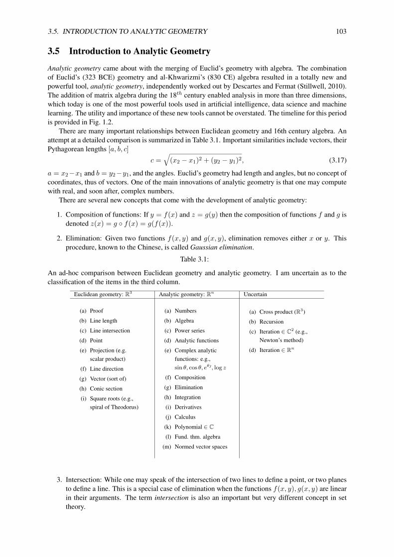
3.5. INTRODUCTION TO ANALYTIC GEOMETRY 103
3.5 Introduction to Analytic Geometry
Analytic geometry came about with the merging of Euclid’s geometry with algebra. The combinationof Euclid’s (323 BCE) geometry and al-Khwarizmi’s (830 CE) algebra resulted in a totally new andpowerful tool, analytic geometry, independently worked out by Descartes and Fermat (Stillwell, 2010).The addition of matrix algebra during the 18th century enabled analysis in more than three dimensions,which today is one of the most powerful tools used in artificial intelligence, data science and machinelearning. The utility and importance of these new tools cannot be overstated. The timeline for this periodis provided in Fig. 1.2.
There are many important relationships between Euclidean geometry and 16th century algebra. Anattempt at a detailed comparison is summarized in Table 3.1. Important similarities include vectors, theirPythagorean lengths [a, b, c]
c =√
(x2 − x1)2 + (y2 − y1)2, (3.17)
a = x2−x1 and b = y2−y1, and the angles. Euclid’s geometry had length and angles, but no concept ofcoordinates, thus of vectors. One of the main innovations of analytic geometry is that one may computewith real, and soon after, complex numbers.
There are several new concepts that come with the development of analytic geometry:
1. Composition of functions: If y = f(x) and z = g(y) then the composition of functions f and g isdenoted z(x) = g f(x) = g(f(x)).
2. Elimination: Given two functions f(x, y) and g(x, y), elimination removes either x or y. Thisprocedure, known to the Chinese, is called Gaussian elimination.
Table 3.1:
An ad-hoc comparison between Euclidean geometry and analytic geometry. I am uncertain as to theclassification of the items in the third column.
Euclidean geometry: R3 Analytic geometry: Rn Uncertain
(a) Proof
(b) Line length
(c) Line intersection
(d) Point
(e) Projection (e.g.scalar product)
(f) Line direction
(g) Vector (sort of)
(h) Conic section
(i) Square roots (e.g.,spiral of Theodorus)
(a) Numbers
(b) Algebra
(c) Power series
(d) Analytic functions
(e) Complex analyticfunctions: e.g.,sin θ, cos θ, eθ, log z
(f) Composition
(g) Elimination
(h) Integration
(i) Derivatives
(j) Calculus
(k) Polynomial ∈ C(l) Fund. thm. algebra
(m) Normed vector spaces
(a) Cross product (R3)
(b) Recursion
(c) Iteration ∈ C2 (e.g.,Newton’s method)
(d) Iteration ∈ Rn
3. Intersection: While one may speak of the intersection of two lines to define a point, or two planesto define a line. This is a special case of elimination when the functions f(x, y), g(x, y) are linearin their arguments. The term intersection is also an important but very different concept in settheory.

104 CHAPTER 3. STREAM 2: ALGEBRAIC EQUATIONS
4. Vectors: Analytic geometry provides the concept of a vector (see Appendix A), as a line withlength and orientation (i.e., direction). Analytic geometry defines vectors in any number of di-mensions, as ordered sets of points.
5. Analytic geometry extends the ideas of Euclidean geometry with the introduction of the scalar(dot) product of two vectors f ·g, and the vector (cross) product f×g (see Fig. 3.4).
What algebra also added to geometry was the ability to compute with complex numbers. For exam-ple, the length of a line (Eq. 3.17) was measured in Geometry with a compass: numbers played no role.Once algebra was available, the line’s Euclidean length could be computed numerically, directly fromthe coordinates of the two ends, defined by the 3-vector
e = xx + yy + zz = [x, y, z]T ,
which represents a point at (x, y, z) ∈ R3 ⊂ C3 in three dimensions, having direction, from the origin(0, 0, 0) to (x, y, z). An alternative matrix notation is e = [x, y, z]T , a column vector of three numbers.These two notations are different ways of representing vector e.
By defining the vector, analytic geometry allows Euclidean geometry to become quantitative, beyondthe physical drawing of an object (e.g., a sphere, triangle or line). With analytic geometry we have theEuclidean concept of a vector, a line having a magnitude (length) and direction, but analytic, defined interms of physical coordinates (i.e., numbers). The difference between two vectors defines a third vector,a concept already present in Euclidean geometry. For the first time, complex numbers were allowed intogeometry (but rarely used before Cauchy and Riemann).
3.5.1 Generalized vector product
As shown in Fig. 3.4, any two vectors A,B ∈ x, y, define a plane. There are two types of vectorproducts:14 the 1) scalar product A ·B = ||A|| ||B|| cos θ ∈ R and 2) vector wedge product A ∧B =||A|| ||B|| sin θ ∈ R, each a real scalar. As show in the figure, these two products form a right triangle,thus may be naturally merged, defining the generalize vector productA ·B+ A∧B = ||A|| ‖|B||eθ.
θ
L∗
A ·B = ||A|| ||B|| cos θ ∈ R
C = A ∧B z = ||A|| ||B|| sin θ z ∈ R
A∧B
A
B
Vector product: ⊥ AB plane
Scalar product: InAB plane
yx
z
Figure 3.4: Vectors A,B,C are used to define the scalar product A · B ∈ R, vector wedge product A ∧ B ∈ R andtriple wedge product C · (A ∧ B). The vector wedge product is the same as the vector cross product except the output isa scalar rather than a vector. As shown in the figure, the scalar dot and vector wedge products complement each other sinceone is proportional to the sin θ of the angle θ between them, and the other to the cos θ. The scalar product computes theprojection of one vector on the other (the length of the base of the triangle formed by the two vectors), while the vector wedgeproduct A ∧ B computes the area of the parallelogram (Area=base·height =2A ·B L∗) formed by the two vectors. Thus|A ·B|2 + |A ∧B|2 = ||A||2||B||2. The scalar triple product C · (A×B) is the volume of the parallelepiped (i.e., prism)defined by the three vectorsA,B and C. When all the angles are 90, the volume becomes a cuboid (p. 207).
14https://en.wikipedia.org/wiki/Bivector

3.5. INTRODUCTION TO ANALYTIC GEOMETRY 105
Scalar product of two vectors: When using algebra, many concepts, obvious with Euclid’s geometry,may be made precise. There are many examples of how algebra extends Euclidean geometry, the mostbasic being the scalar product (aka, dot product) between vectors x ∈ R3,κ ∈ C3
x · κ = (xx + yy + zz) · (αx + βy + γz), ∈ C= αx+ βy + γz.
Scalar products play an important role in vector algebra and calculus (see Appendix A.2, p. 253).In matrix notation the scalar product is written as (p. 207)
x · κ =
xyz
T αβ
γ
=[x, y, z
] αβγ
= αx+ βy + γz. (3.18)
If κ(s) ∈ C3 is a function of complex function of frequency s, then the scalar product is complexfunction of s.
Norm (length) of a vector: The norm of a vector (Appendix A.2, p. 254)
||e|| ≡ +√
e · e ≥ 0
is defined as the positive square root of the scalar product of the vector with itself. This is a generalizationof the length, in any number of dimensions, forcing the sign of the square-root to be non-negative. Thelength is a concept of Euclidean geometry, and it must always be positive and real. A complex (ornegative) length is not physically meaningful. More generally, the Euclidean length of a line is given asthe norm of the difference between two real vectors e1, e2 ∈ R
||e1 − e2||2 = (e1 − e2) · (e1 − e2)= (x1 − x2)2 + (y1 − y2)2 + (z1 − z2)2 ≥ 0.
From this formula we see that the norm of the difference of two vectors is simply a compact expressionfor the Euclidean length. A zero-length vector, such as is a point, is the result of the fact that
||x− x||2 = (x− x) · (x− x),
is zero.
Integral definition of a scalar product: Up to this point, following Euclid, we have only considereda vector to be a set of elements xn ∈ R, index over n ∈ N, as defining a linear vector space withscalar product x · y, with the scalar product defining the norm or length of the vector ||x|| =
√x · x.
Given the scalar product, the norm naturally follows.At this point an obvious question presents itself: Can we extend our definition of vectors to differ-
entiable functions (i.e., f(t) and g(t)), indexed over t ∈ R, with coefficients labeled by t ∈ R, ratherthan by n ∈ N? Clearly, if the functions are analytic, there is no obvious reason why this should be aproblem, since analytic functions may be represented by a convergent series having Taylor coefficients,thus are integrable term by term.
Specifically, under certain conditions, the function f(t) may be thought of as a vector, defining anormed vector space. This intuitive and somewhat obvious idea is powerful. In this case the scalarproduct can be defined in terms of the integral
f(t) · g(t) =∫tf(t)g(t)dt
= ||f(t)|| ||g(t)|| cos θ.
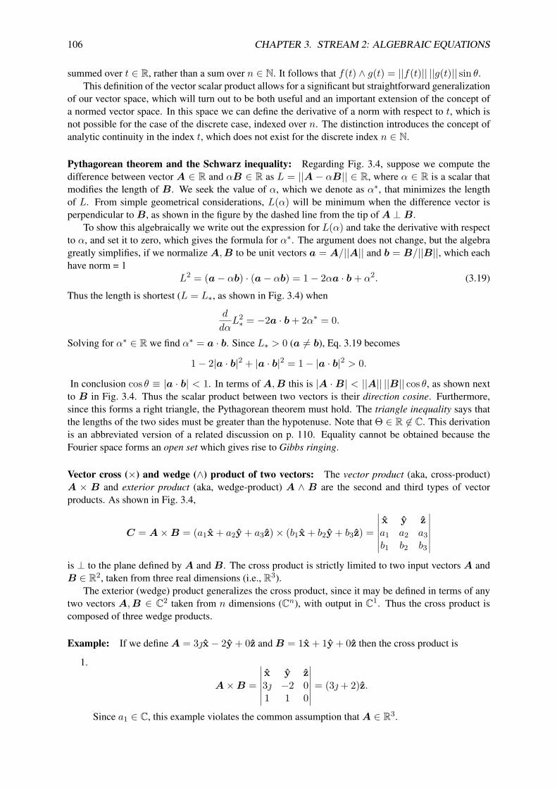
106 CHAPTER 3. STREAM 2: ALGEBRAIC EQUATIONS
summed over t ∈ R, rather than a sum over n ∈ N. It follows that f(t) ∧ g(t) = ||f(t)|| ||g(t)|| sin θ.This definition of the vector scalar product allows for a significant but straightforward generalization
of our vector space, which will turn out to be both useful and an important extension of the concept ofa normed vector space. In this space we can define the derivative of a norm with respect to t, which isnot possible for the case of the discrete case, indexed over n. The distinction introduces the concept ofanalytic continuity in the index t, which does not exist for the discrete index n ∈ N.
Pythagorean theorem and the Schwarz inequality: Regarding Fig. 3.4, suppose we compute thedifference between vector A ∈ R and αB ∈ R as L = ||A − αB|| ∈ R, where α ∈ R is a scalar thatmodifies the length of B. We seek the value of α, which we denote as α∗, that minimizes the lengthof L. From simple geometrical considerations, L(α) will be minimum when the difference vector isperpendicular toB, as shown in the figure by the dashed line from the tip ofA ⊥ B.
To show this algebraically we write out the expression for L(α) and take the derivative with respectto α, and set it to zero, which gives the formula for α∗. The argument does not change, but the algebragreatly simplifies, if we normalize A,B to be unit vectors a = A/||A|| and b = B/||B||, which eachhave norm = 1
L2 = (a− αb) · (a− αb) = 1− 2αa · b+ α2. (3.19)
Thus the length is shortest (L = L∗, as shown in Fig. 3.4) when
d
dαL2∗ = −2a · b+ 2α∗ = 0.
Solving for α∗ ∈ R we find α∗ = a · b. Since L∗ > 0 (a 6= b), Eq. 3.19 becomes
1− 2|a · b|2 + |a · b|2 = 1− |a · b|2 > 0.
In conclusion cos θ ≡ |a · b| < 1. In terms of A,B this is |A ·B| < ||A|| ||B|| cos θ, as shown nextto B in Fig. 3.4. Thus the scalar product between two vectors is their direction cosine. Furthermore,since this forms a right triangle, the Pythagorean theorem must hold. The triangle inequality says thatthe lengths of the two sides must be greater than the hypotenuse. Note that Θ ∈ R 6∈ C. This derivationis an abbreviated version of a related discussion on p. 110. Equality cannot be obtained because theFourier space forms an open set which gives rise to Gibbs ringing.
Vector cross (×) and wedge (∧) product of two vectors: The vector product (aka, cross-product)A × B and exterior product (aka, wedge-product) A ∧ B are the second and third types of vectorproducts. As shown in Fig. 3.4,
C = A×B = (a1x + a2y + a3z)× (b1x + b2y + b3z) =
∣∣∣∣∣∣∣x y za1 a2 a3b1 b2 b3
∣∣∣∣∣∣∣is ⊥ to the plane defined by A and B. The cross product is strictly limited to two input vectors A andB ∈ R2, taken from three real dimensions (i.e., R3).
The exterior (wedge) product generalizes the cross product, since it may be defined in terms of anytwo vectors A,B ∈ C2 taken from n dimensions (Cn), with output in C1. Thus the cross product iscomposed of three wedge products.
Example: If we defineA = 3x− 2y + 0z andB = 1x + 1y + 0z then the cross product is
1.
A×B =
∣∣∣∣∣∣∣x y z3 −2 01 1 0
∣∣∣∣∣∣∣ = (3+ 2)z.
Since a1 ∈ C, this example violates the common assumption thatA ∈ R3.

3.5. INTRODUCTION TO ANALYTIC GEOMETRY 107
2. The wedge product A ∧ B takes two vectors and returns a scalar, which is the magnitude of avector ⊥ to the plane defined by the two input vectors (see Fig. 3.4). It is defined as
A ∧B =∣∣∣∣∣a1 b1a2 b2
∣∣∣∣∣ =∣∣∣∣∣ 3 1−2 1
∣∣∣∣∣= (3x− 2y) ∧ (x + y)
= 3 · 0:0x ∧ x− 2y ∧ x + 3x ∧ y− 2:0y ∧ y
= (3+ 2)||x ∧ y||= (3+ 2)||z|| = 3+ 2.
This defines for a compact and useful algebra (Hestenes, 2003).From the above example we see that the absolute value of the wedge product |a ∧ b| = ||a × b||,
namely|(a2y + a3z) ∧ (b2y + b3z)| = ||a × b||.
The wedge product is especially useful because it is zero when the two vectors are co-linear, namelyx ∧ x = 0 and x ∧ y = 1, where x, y are unit vectors. Since
a · b = ||a|| ||b|| cos θ and a ∧ b = ||a|| ||b|| sin θ,
it follows thata · b + a ∧ b = ||a|| ||b|| eθ,
which may be viewed as the complex scalar product, with the right hand side the polar form.The main advantage of the “wedge” product is that it is valid in n ≥ 3 dimensions, since it is defined
for any two vectors, in any number of dimensions. Like the cross product, the magnitude of the wedgeproduct is equal to the area of the trapezoid formed by the two vectors.
Scalar triple product: The triple of a third vector C with the vector productA×B ∈ R is
C · (A×B) =
∣∣∣∣∣∣∣c1 c2 c3a1 a2 a3b1 b2 b3
∣∣∣∣∣∣∣ ∈ R3,
which equals the volume of a parallelepiped.
Impact of Analytic Geometry: The most obvious impact of analytic geometry was its detailed anal-ysis of the conic sections, using algebra rather than drawings via a compass and ruler. An importantexample is the composition of the line and circle, a venerable construction, presumably going back tobefore Diophantus (250CE). Once algebra was invented, the composition could be done using formulas.With this analysis came complex numbers.
The first two mathematicians to appreciate this mixture of Euclid’s geometry and the new algebrawere Fermat and Descartes; soon Newton contributed to this effort by the addition of physics (e.g.,calculations in acoustics, orbits of the planets, and the theory of gravity and light, significant conceptsfor 1687.
Given these new methods, many new solutions to problems emerged. The complex roots of polyno-mials continued to appear, without any obvious physical meaning. Complex numbers seem to have beenviewed as more of an inconvenience than a problem. Newton’s solution to this dilemma was to simplyignore the “imaginary” cases (Stillwell, 2010, p. 115-119).

108 CHAPTER 3. STREAM 2: ALGEBRAIC EQUATIONS
3.5.2 Development of Analytic Geometry
Intersection and Gaussian elimination: The first “algebra” (al-jabr) is credited to al-Khwarizmi (830CE). Its invention advanced the theory of polynomial equations in one variable, Taylor series, and com-position versus intersections of curves. The solution of the quadratic equation had been worked outthousands of years earlier, but with algebra a general solution could be defined. The Chinese had foundthe way to solve several equations in several unknowns, for example, finding the values of the intersec-tion of two circles. With the invention of algebra by al-Khwarizmi, a powerful tool became available tosolve more difficult problems.
Composition and Elimination In algebra there are two contrasting operations on functions: compo-sition and elimination.
Composition: Composition is the merging of functions, by feeding one into the other. If the twofunctions are f, g then their composition is indicated by f g, meaning the function y = f(x) issubstituted into the function z = g(y), giving z = g(f(x)).
Composition is not limited to linear equations, even though that is where it is most frequently ap-plied. To compose two functions, one must substitute one equation into the other. That requires solvingfor that substitution variable, which is not always possible in the case of nonlinear equations. However,many tricks are available that may work around this restriction. For example, if one equation is in x2
and the other in x3 or√x, it may be possible to multiply the first by x or square the second. The point
is that one of the variables must be isolated so that when it is substituted into the other equations, thevariable is removed from the mix.
Example: Let y = f(x) = x2 − 2 and z = g(y) = y + 1. Then
g f = g(f(x)) = (x2 − 2) + 1 = x2 − 1. (3.20)
In general composition does not commute (i.e., fg 6= gf ), as is easily demonstrated. Swappingthe order of composition for our example gives
f g = f(g(y)) = z2 − 2 = (y + 1)2 − 2 = y2 + 2y − 1. (3.21)
Intersection: Complementary to composition is intersection (i.e., decomposition). For example, theintersection of two lines is defined as the point where they meet. This is not to be confused with findingroots. A polynomial of degree N has N roots, but the points where two polynomials intersect hasnothing to do with the roots of the polynomials. The intersection is a function (equation) of lowerdegree, implemented by Gaussian elimination.
Intersection of two lines Unless they are parallel, two lines meet at a point. In terms of linear algebrathis may be written as two linear equations15 (on the left), along with the intersection point [x1, x2]T ,given by the inverse of the 2× 2 set of equations (on the right)[
a bc d
] [x1x2
]=[y1y2
] [x1x2
]= 1
∆
[d −b−c a
] [y1y2
]. (3.22)
By substituting the expression for the intersection point [x1,x2]T into the original equation, we see thatit satisfies the equations. Thus the equation on the right is the solution to the equation on the left.
15When writing the equation Ax = y in matrix format, the two equations are ax1 + bx2 = y1 and dx1 + ex2 = y2 withunknowns (x1, x2), whereas in the original equations ay + bx = c and dy + ex = f , they were y, x. Thus in matrix format,the names are changed. The first time you see this scrambling of variables, it can be confusing.

3.5. INTRODUCTION TO ANALYTIC GEOMETRY 109
Note the structure of the inverse: 1) The diagonal values (a, d) are swapped, 2) the off-diagonalvalues (b, c) are negated and 3) the 2× 2 matrix is divided by the determinant ∆ = ad− bc. If ∆ = 0,there is no solution. When the determinant is zero (∆ = 0), the slopes of the two lines
slope = dx2dx1
= b
a= d
c
are equal, thus the lines are parallel. Only if the slopes differ can there be a unique solution.
Exercise: Show that the equation on the right is the solution of the equation on the left. Solution: Bya direct substitution (composition) of the right equation into the left equation[
a bc d
]· 1
∆
[d −b−c a
] [y1y2
],= 1
∆
[ad− bc −ab+ abcd− cd −cb+ ad
]= 1
∆
[∆ 00 ∆
],
which gives the identity matrix.
Algebra will give the solution when geometry cannot. When the two curves fail to intersect on thereal plane, the solution still exists, but is complex valued. In such cases, geometry, which only considersthe real solutions, fails. For example, when the coefficients [a, b, c, d] are complex, the solution exists,but the determinant can be complex. Thus algebra is much more general than geometry. Geometry failswhen the solution has a complex intersection.
A system of linear equations Ax = y has many interpretations, and one should not be biased by thenotation. As engineers we are trained to view x as the input and y as the output, in which case theny = Ax seems natural, much like the functional relation y = f(x). But what does the linear relationx = Ay mean, when x is the input? The obvious answer is that y = A−1x. But when working withsystems of equations, there are many uses of equations, and we need to become more flexible in ourinterpretation. For example y = A2x has a useful meaning, and in fact we saw this type of relationshipwhen working with Pell’s equation (p. 57) and the Fibonacci sequence (p. 59). As another exampleconsider [
z1z2
]=[a1x a1ya2x a2y
] [xy
],
which is reminiscent of a three-dimensional surface z = f(x, y). We shall find that such generalizationsare much more than a curiosity.
3.5.3 Applications of scalar products
Another important example of algebraic expressions in mathematics is Hilbert’s generalization of thePythagorean theorem (Eq. 1.1), known as the Schwarz inequality, is shown in Fig. 3.5. What is specialabout this generalization is that it proves that when the vertex is 90, the Euclidean length of the leg isminimum.
Vectors may be generalized to have∞ dimensions: U,V = [v1, v2, · · · , v∞]). The Euclidean innerproduct (i.e., scalar product) between two such vectors generalizes the finite dimensional case
U ·V =∞∑k=1
ukvk.
As with the finite case, the norm ||U|| =√
U ·U =√∑
u2k is the scalar product of the vector with
itself, defining the length of the infinite component vector. Obviously there is an issue of convergence,if the norm for the vector is to have a finite length.
It is a somewhat arbitrary requirement that a, b, c ∈ R for the Pythagorean theorem (Eq. 1.1). Thisseems natural enough since the sides are lengths. But, what if they are taken from the complex numbers,as for the lossy vector wave equation, or the lengths of vectors in Cn? Then the equation generalizes to
c · c = ||c||2 =n∑k=1|ck|2,
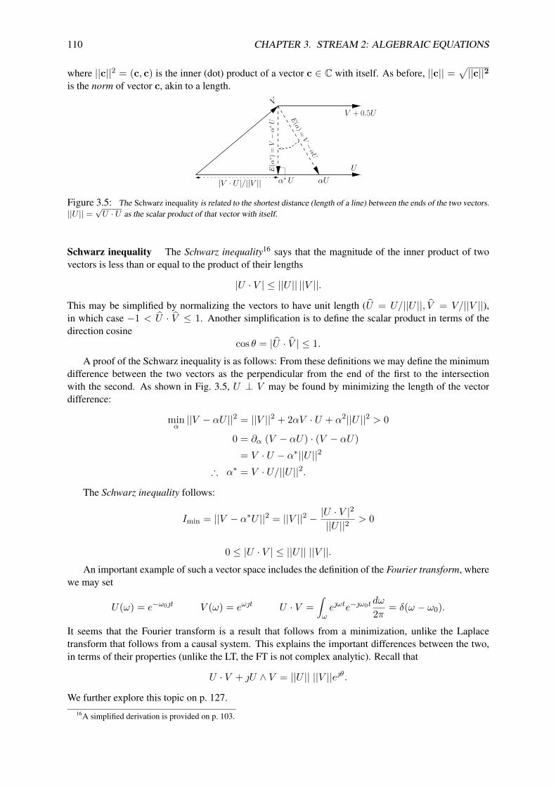
110 CHAPTER 3. STREAM 2: ALGEBRAIC EQUATIONS
where ||c||2 = (c, c) is the inner (dot) product of a vector c ∈ C with itself. As before, ||c|| =√||c||2
is the norm of vector c, akin to a length.
V + 0.5UE(α) =V−αU
|V · U |/||V ||
UE(α∗ )
=V−α∗U
V
α∗U αU
Figure 3.5: The Schwarz inequality is related to the shortest distance (length of a line) between the ends of the two vectors.||U || =
√U · U as the scalar product of that vector with itself.
Schwarz inequality The Schwarz inequality16 says that the magnitude of the inner product of twovectors is less than or equal to the product of their lengths
|U · V | ≤ ||U || ||V ||.
This may be simplified by normalizing the vectors to have unit length (U = U/||U ||, V = V/||V ||),in which case −1 < U · V ≤ 1. Another simplification is to define the scalar product in terms of thedirection cosine
cos θ = |U · V | ≤ 1.A proof of the Schwarz inequality is as follows: From these definitions we may define the minimum
difference between the two vectors as the perpendicular from the end of the first to the intersectionwith the second. As shown in Fig. 3.5, U ⊥ V may be found by minimizing the length of the vectordifference:
minα||V − αU ||2 = ||V ||2 + 2αV · U + α2||U ||2 > 0
0 = ∂α (V − αU) · (V − αU)= V · U − α∗||U ||2
∴ α∗ = V · U/||U ||2.
The Schwarz inequality follows:
Imin = ||V − α∗U ||2 = ||V ||2 − |U · V |2
||U ||2> 0
0 ≤ |U · V | ≤ ||U || ||V ||.An important example of such a vector space includes the definition of the Fourier transform, where
we may set
U(ω) = e−ω0t V (ω) = eωt U · V =∫ωeωte−ω0tdω
2π = δ(ω − ω0).
It seems that the Fourier transform is a result that follows from a minimization, unlike the Laplacetransform that follows from a causal system. This explains the important differences between the two,in terms of their properties (unlike the LT, the FT is not complex analytic). Recall that
U · V + U ∧ V = ||U || ||V ||eθ.
We further explore this topic on p. 127.16A simplified derivation is provided on p. 103.

3.5. INTRODUCTION TO ANALYTIC GEOMETRY 111
3.5.4 Gaussian Elimination
The method for finding the intersection of equations is based on the recursive elimination of all thevariables but one. This method, known as Gaussian elimination (Appendix 5, p. 257), works acrossa broad range of cases, but may be defined as a systematic algorithm when the equations are linear inthe variables (Strang et al., 1993). Rarely do we even attempt to solve problems in several variables ofdegree greater than 1. But Gaussian eliminations may still work in such cases (Stillwell, 2010, p. 90).
In Appendix A.2.3 (p. 260) the inverse of a 2 × 2 linear system of equations is derived. Even fora 2 × 2 case, the general solution requires a great deal of algebra. Working out a numeric example ofGaussian elimination is more instructive. For example, suppose we wish to find the intersection of thetwo equations
x− y = 32x+ y = 2.
This 2× 2 system of equations is so simple that you may immediately visualize the solution: By addingthe two equations, y is eliminated, leaving 3x = 5. But doing it this way takes advantage of the specificexample, and we need a method for larger systems of equations. We need a generalized (algorithmic)approach. This general approach is called Gaussian elimination.
Start by writing the equations in matrix form (note this is not of the form Ax = y)[1 −12 1
] [xy
]=[32
]. (3.23)
Next, eliminate the lower left term (2x) using a scaled version of the upper left term (x). Specifically,multiply the first equation by −2, add it to the second equation, replacing the second equation with theresult. This gives [
1 −10 3
] [xy
]=[
32− 3 · 2
]=[
3−4
]. (3.24)
Note that the top equation did not change. Once the matrix is “upper triangular” (zero below the diag-onal) you have the solution. Starting from the bottom equation, y = −4/3. Then the upper equationgives x− (−4/3) = 3, or x = 3− 4/3 = 5/3.
In principle, Gaussian elimination is easy, but if you make a calculation mistake along the way, itis very difficult to find your error. The method requires a lot of mental labor, with a high probabilityof making a mistake. Thus you do not want to apply this method every time. For example, supposethe elements are complex numbers, or polynomials in some other variable such as frequency. Once thecoefficients become more complicated, the seemingly trivial problem becomes corrosive. There is amuch better way, that is easily verified, which puts all the numerics at the end, in a single step.
The above operations may be automated by finding a carefully chosen upper-diagonalize matrix G.For example, define the “Gaussian matrix” that removes the element 2 in A.
Let
G =[1 0a 1
](3.25)
Multiplying Eq. 3.23 by G, we find[1 0a 1
] [1 −12 1
] [xy
]=[
1 −1a+ 2 1− a
] [xy
]=[1 0a 1
] [32
]=[
33a+ 2
](3.26)
thus we obtain Eq. 3.24 if we let a = −2 (we choose a to force the lower-left to be zero). At this pointwe can either back-substitute and obtain the solution, as we did above, or find a matrix L that finishesthe job, by removing elements above the diagonal. The key is that the determinant of this matrix is 1.

112 CHAPTER 3. STREAM 2: ALGEBRAIC EQUATIONS
Exercise: Using G and A from the discussion above, show that det(G) = det(GA) = 3.Solution: We wish to show that det(GA) = detG · det(A). A common notation is to denote
det(A) = |A|. The two sides of the identity are
|A| = det[1 −12 1
]= 1 + 2 = 3, |GA| = det
[1 −10 3
]= 3,
and |G| = 1. Thus |GA| = |G||A| = 3.
Matrix inverse: In Appendix A.2.3, p. 260, the inverse of a general 2 × 2 matrix takes three steps:1) swap the diagonal elements, 2) reverse the signs of the off-diagonal elements and 3) divide by thedeterminant ∆ = ab− cd. Specifically[
a bc d
]−1
= 1∆
[d −b−c a
]. (3.27)
There are very few things that you must memorize, but the inverse of a 2× 2 is one of them. It needs tobe in your mental tool-kit, like the completion of squares (p. 73).
While it is difficult to compute the inverse matrix from scratch (Appendix 5), it takes only a fewseconds (four dot products) to verify it (steps 1 and 2)[
a bc d
] [d −b−c a
]=[ad− bc −ab+ abcd− cd −bc+ ad
]=[∆ 00 ∆
]. (3.28)
Thus dividing by the determinant gives the 2 × 2 identity matrix. A good strategy (don’t trust yourmemory) is to write down the inverse as best you recall, and then verify.
Using the 2× 2 matrix inverse on our example (Eq. 3.23), we find[xy
]= 1
1 + 2
[1 1−2 1
] [32
]= 1
3
[5
−6 + 2
]=[
5/3−4/3
]. (3.29)
If you use this method, you will rarely (never) make a mistake, and the solution is easily verified. Eitheryou can check the numbers in the inverse, as was done in Eq. 3.28, or you can substitute the solutionback into the original equation.
Augmented matrix: There is one minor notational improvement. Rather than writing th matrix equa-tion as Eq. 3.23 (Ax = y) we place the y vector next to the elements of A, to remove the equal sign,which is cumbersome. In this case we write GAaug
GAaug =[
1 0−2 1
] [1 −1 32 1 2
]=[
1 −1 30 3 −4
].

3.6. EXERCISES AE-2 113
3.6 Exercises AE-2
Topic of this homework:
Linear systems of equations; Gaussian elimination; Matrix permutations; Overspecified systems of equa-tions; Analytic geometry; Ohm’s law; Two-port networks
Deliverable: Answers to problems
Nonlinear (quadratic) to linear equations
Problem # 1: Nonlinear (quadratic) to linear equationsIn the following problems we deal with algebraic equations in more than one variable, that are notlinear equations. For example, the circle x2 + y2 = 1 is just such an equation. It may be solved fory(x) = ±
√1− x2.
Example: If we let z+ = x + y = x + √
1− x2 = eθ, we obtain the equation for half a circle(y > 0). The entire circle is described by the magnitude of z, as |z|2 = (x+ y)(x− y) = 1.
–Q 1.1: Given the curve defined by the equation:
x2 + xy + y2 = 1
–Q 1.2: Find the function y(x).
–Q 1.3: Using Matlab/Octave, plot y(x), and describe the graph.
–Q 1.4: What is the name of this curve?
–Q 1.5: Find the solution (in x, p, and q) to the following equations:
x+ y= p
xy = q
–Q 1.6: Find an equation that is linear in y starting from equations that are quadratic (2nddegree) in the two unknownsx, y:
x2 + xy + y2 = 1 (3.1)
4x2 + 3xy + 2y2 = 3 (3.2)
–Q 1.7: Compose the two quadratic equations
x2 + xy + y2= 12x2 + xy = 1
and describe the results.

114 CHAPTER 3. STREAM 2: ALGEBRAIC EQUATIONS
Gaussian elimination
Problem # 2: Gaussian elimination
–Q 2.1: Find the inverse of
A =[1 24 3
].
–Q 2.2: Verify that A−1A = AA−1 =[1 00 1
].
Problem # 3: Find the solution to the following 3x3 matrix equation Ax = b by Gaussianelimination. Show your intermediate steps. You can check your work at each step using Oc-tave/Matlab. 1 1 −1
3 1 11 −1 4
x1x2x3
=
198
.–Q 3.1 Show (i.e., verify) that the first GE matrix G1, which zeros out all entries in the first
column, is given by
G1 =
1 0 0−3 1 0−1 0 1
Identify the elementary row operations that this matrix performs.
–Q 3.2 Find a second GE matrix, G2, to put G1A in upper triangular form. Identify theelementary row operations that this matrix performs.
–Q 3.3 Find a third GE matrix, G3, which scales each row so that its leading term is 1.Identify the elementary row operations that this matrix performs.
–Q 3.4: Finally, find the last GE matrix, G4, that subtracts a scaled version of row 3 fromrow 2, and scaled versions of rows 2 and 3 from row 1, such that you are left with the identitymatrix (G4G3G2G1A = I).
–Q 3.5: Solve for x1, x2, x3T using the augmented matrix formatG4G3G2G1A|b (whereA|b is the augmented matrix). Note that if you’ve performed the preceding steps correctly,x = G4G3G2G1b.
Permutations and Pivots
Problem # 4: Permutations and Pivots 1. Find the pivot matrix G that rescales the third row ofthe augmented matrix A|b by 1/3.
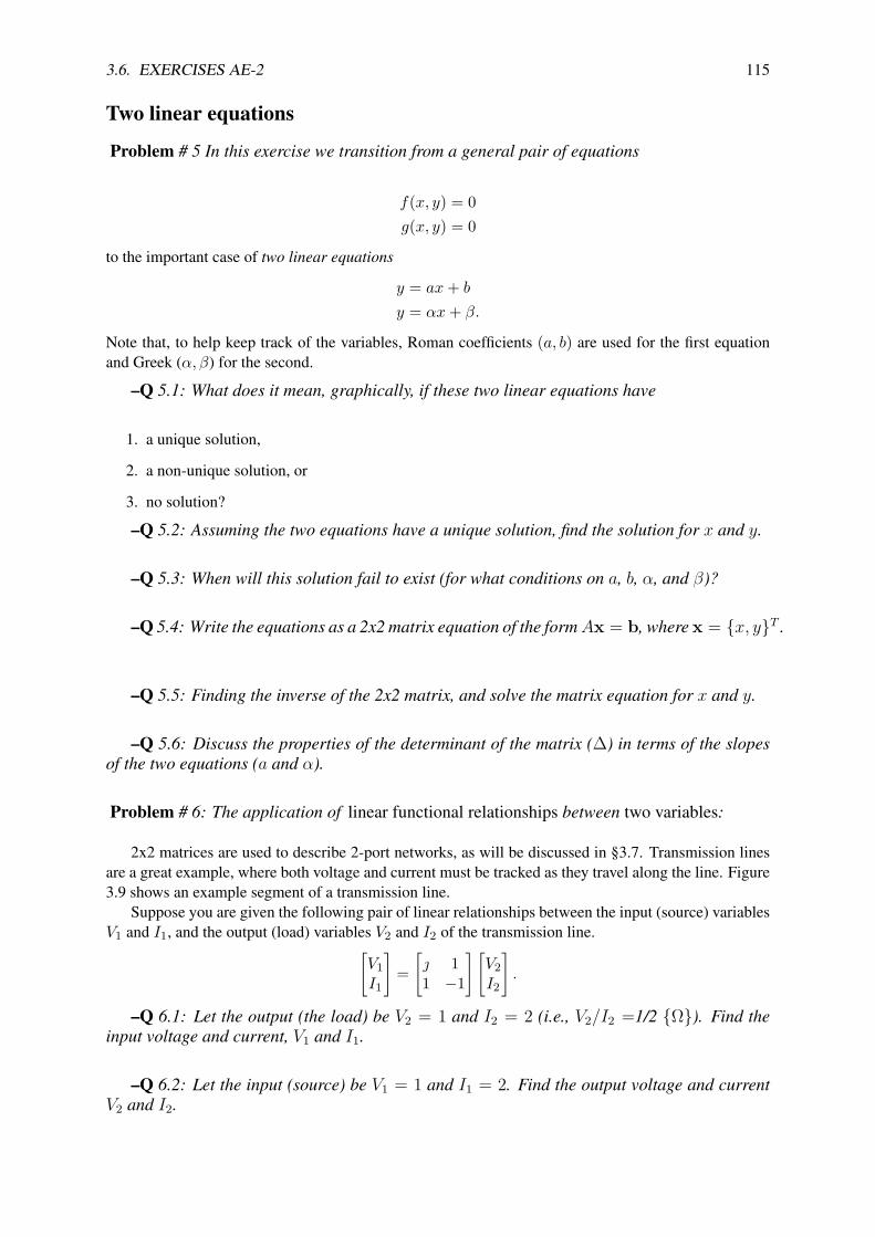
3.6. EXERCISES AE-2 115
Two linear equations
Problem # 5 In this exercise we transition from a general pair of equations
f(x, y) = 0g(x, y) = 0
to the important case of two linear equations
y = ax+ b
y = αx+ β.
Note that, to help keep track of the variables, Roman coefficients (a, b) are used for the first equationand Greek (α, β) for the second.
–Q 5.1: What does it mean, graphically, if these two linear equations have
1. a unique solution,
2. a non-unique solution, or
3. no solution?
–Q 5.2: Assuming the two equations have a unique solution, find the solution for x and y.
–Q 5.3: When will this solution fail to exist (for what conditions on a, b, α, and β)?
–Q 5.4: Write the equations as a 2x2 matrix equation of the formAx = b, where x = x, yT .
–Q 5.5: Finding the inverse of the 2x2 matrix, and solve the matrix equation for x and y.
–Q 5.6: Discuss the properties of the determinant of the matrix (∆) in terms of the slopesof the two equations (a and α).
Problem # 6: The application of linear functional relationships between two variables:
2x2 matrices are used to describe 2-port networks, as will be discussed in §3.7. Transmission linesare a great example, where both voltage and current must be tracked as they travel along the line. Figure3.9 shows an example segment of a transmission line.
Suppose you are given the following pair of linear relationships between the input (source) variablesV1 and I1, and the output (load) variables V2 and I2 of the transmission line.[
V1I1
]=[ 11 −1
] [V2I2
].
–Q 6.1: Let the output (the load) be V2 = 1 and I2 = 2 (i.e., V2/I2 =1/2 Ω). Find theinput voltage and current, V1 and I1.
–Q 6.2: Let the input (source) be V1 = 1 and I1 = 2. Find the output voltage and currentV2 and I2.

116 CHAPTER 3. STREAM 2: ALGEBRAIC EQUATIONS
L = ρA(x)
V2V1 +
−
+
−
I2I1
C = ηPA(x)
Figure 3.6: This figure shows a cell from an LC transmission line. The index 1 is at the input on the left and 2 representsthe output, on the right. This figure is discussed in §3.7.3 (p. 126).
Linear equations with three unknowns
Problem # 7: This problem is similar to the previous problem, except we consider 3 dimen-sions. Consider two linear equations in unknowns x, y, z, representing planes:
a1x+ b1y + z = c1 (3.3)
a2x+ b2y + z = c2 (3.4)
–Q 7.1: In terms of the geometry (i.e., think graphically), under what conditions do thesetwo linear equations have (a) a unique solution, (b) a non-unique solution, or (c) no solution?
–Q 7.2: Do you know what is meant by the slope of a plane? Can you define it?
–Q 7.3: Given 2 equations in 3 unknowns, the closest we can come to a ‘unique’ solutionis a line (describing the intersection of the planes) rather than a single point. This line is anequation in (x, y), (y, z), or (x, z). Find a solution in terms of x and y by substituting oneequation into the other.
Problem # 8: Now consider the intersection of the planes at some arbitrary constant height,z = z0.
–Q 8.1: Write the modified plane equations as a 2x2 matrix equation in the form Ax = bwhere x = x, yT , and find the unique solution in x and y using matrix operations.
–Q 8.2: Assuming the two equations have a unique solution, find the solution for x and y.
–Q 8.3: When will this solution fail to exist (for what conditions on a1, a2, b1, b2, etc.)?
–Q 8.4: Now, write the system of equations as a 3x3 matrix equation in x, y, z given theadditional equation z = z0 (e.g. put it in the form Ax = b where x = x, y, zT ).
Problem # 9: The determinant of a 3x3 matrix is given by∣∣∣∣∣∣∣a11 a12 a13a21 a22 a23a31 a32 a33
∣∣∣∣∣∣∣ = a11
∣∣∣∣∣a22 a23a32 a33
∣∣∣∣∣− a12
∣∣∣∣∣a21 a23a31 a33
∣∣∣∣∣+ a13
∣∣∣∣∣a21 a22a31 a32
∣∣∣∣∣
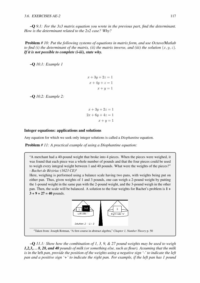
3.6. EXERCISES AE-2 117
–Q 9.1: For the 3x3 matrix equation you wrote in the previous part, find the determinant.How is the determinant related to the 2x2 case? Why?
Problem # 10: Put the following systems of equations in matrix form, and use Octave/Matlabto find (i) the determinant of the matrix, (ii) the matrix inverse, and (iii) the solution (x, y, z).If it is not possible to complete (i-iii), state why.
–Q 10.1: Example 1
x+ 3y + 2z = 1x+ 4y + z = 1
x+ y = 1
–Q 10.2: Example 2:
x+ 3y + 2z = 12x+ 6y + 4z = 1
x+ y = 1
Integer equations: applications and solutions
Any equation for which we seek only integer solutions is called a Diophantine equation.
Problem # 11: A practical example of using a Diophantine equation:
“A merchant had a 40-pound weight that broke into 4 pieces. When the pieces were weighed, itwas found that each piece was a whole number of pounds and that the four pieces could be usedto weigh every integral weight between 1 and 40 pounds. What were the weights of the pieces?”- Bachet de Beziriac (1623 CE)a
Here, weighing is performed using a balance scale having two pans, with weights being put oneither pan. Thus, given weights of 1 and 3 pounds, one can weigh a 2-pound weight by puttingthe 1-pound weight in the same pan with the 2-pound weight, and the 3-pound weigh in the otherpan. Then, the scale will be balanced. A solution to the four weights for Bachet’s problem is 1 +3 + 9 + 27 = 40 pounds.
aTaken from: Joseph Rotman, “A first course in abstract algebra,” Chapter 1, Number Theory p. 50
–Q 11.1: Show how the combination of 1, 3, 9, & 27 pound weights may be used to weigh1,2,3,. . . 8, 28, and 40 pounds of milk (or something else, such as flour). Assuming that the milkis in the left pan, provide the position of the weights using a negative sign ‘-’ to indicate the leftpan and a positive sign ‘+’ to indicate the right pan. For example, if the left pan has 1 pound
118 CHAPTER 3. STREAM 2: ALGEBRAIC EQUATIONS
of milk, then 1 pound of milk in the right pan, ‘+1’ will balance the scales.
Hint: It is helpful to write the answer in matrix form. Set the vector of values to be weighed equalto a matrix indicating the pan assignments, multiplied by a vector of the weights [1, 3, 9, 27]T . The panassignments matrix should only contain the values -1 (left pan), +1 (right pan), and 0 (leave out). Youcan indicate these using ‘-’, ‘+’, and blank spaces.
Ohm’s Law
In general, impedance is defined as the ratio of a force over a flow. For electrical circuits, the voltage isthe ‘force’ and the current is the ‘flow.’ Ohm’s law states that the voltage across and the current througha circuit element are related by the impedance of that element (which may be a function of frequency).For resistors, the voltage over the current is called the resistance, and is a constant (e.g. the simplestcase, V/I = R). For inductors and capacitors, the voltage over the current is a frequency-dependentimpedance (e.g. V/I = Z(s), where s is the complex frequency s ∈ C).
As described in Fig. 3.2 (p. 125) the impedance concept also holds in mechanics and acoustics. Inmechanics, the ‘force’ is equal to the mechanical force on an element (e.g. a mass, dashpot, or spring),and the ‘flow’ is the velocity. In acoustics, the ‘force’ is pressure, and the ‘flow’ is the volume velocityor particle velocity of air molecules.
Problem # 12: The resistance of an incandescent (filament) lightbulb, measured cold, is about100 ohms. As it lights up, the resistance of the metal filament increases.Ohm’s law says that the current
V
I= R(T ).
where T is the temperature. In the United States, the voltage is 120 volts (RMS) at 60 [Hz].
–Q 12.1: Find the current when the light is first switched on.
Problem # 13: The power in Watts is the product of the force and the flow.
–Q 13.1: What is the power of the light bulb of this example?
Problem # 14: State the impedance Z(s) of each of the following circuit elements:
–Q 14.1: A resistor with resistance R:
–Q 14.2: An inductor with inductance L:
–Q 14.3: A capacitor with capacitance C:
Problem # 15: Consider what happens at the triple-point of water. As water freezes or thaws,the temperate remains constant at 0 (C°). Once all the water is frozen and more heat is removed,the temperature drops below 0 °. As heat is added, water thaws, but the temperature remainsat 0°.
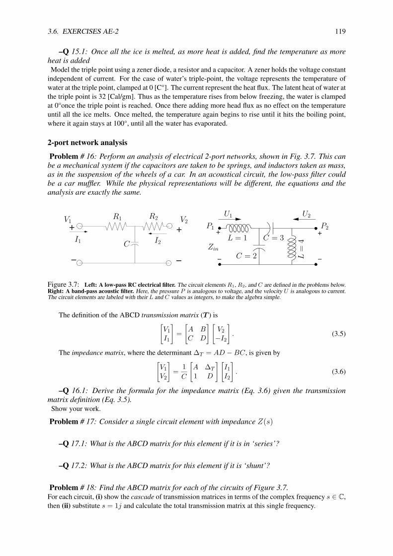
3.6. EXERCISES AE-2 119
–Q 15.1: Once all the ice is melted, as more heat is added, find the temperature as moreheat is addedModel the triple point using a zener diode, a resistor and a capacitor. A zener holds the voltage constant
independent of current. For the case of water’s triple-point, the voltage represents the temperature ofwater at the triple point, clamped at 0 [C°]. The current represent the heat flux. The latent heat of water atthe triple point is 32 [Cal/gm]. Thus as the temperature rises from below freezing, the water is clampedat 0°once the triple point is reached. Once there adding more head flux as no effect on the temperatureuntil all the ice melts. Once melted, the temperature again begins to rise until it hits the boiling point,where it again stays at 100°, until all the water has evaporated.
2-port network analysis
Problem # 16: Perform an analysis of electrical 2-port networks, shown in Fig. 3.7. This canbe a mechanical system if the capacitors are taken to be springs, and inductors taken as mass,as in the suspension of the wheels of a car. In an acoustical circuit, the low-pass filter couldbe a car muffler. While the physical representations will be different, the equations and theanalysis are exactly the same.
+
−
+
−
R1 R2
I1
V1 V2
C I2+
−
+
−
U1
Zin
L = 1 C = 3
C = 2 L=
4
P1 P2
U2
Figure 3.7: Left: A low-pass RC electrical filter. The circuit elements R1, R2, and C are defined in the problems below.Right: A band-pass acoustic filter. Here, the pressure P is analogous to voltage, and the velocity U is analogous to current.The circuit elements are labeled with their L and C values as integers, to make the algebra simple.
The definition of the ABCD transmission matrix (T ) is[V1I1
]=[A BC D
] [V2−I2
]. (3.5)
The impedance matrix, where the determinant ∆T = AD −BC, is given by[V1V2
]= 1C
[A ∆T
1 D
] [I1I2
]. (3.6)
–Q 16.1: Derive the formula for the impedance matrix (Eq. 3.6) given the transmissionmatrix definition (Eq. 3.5).
Show your work.
Problem # 17: Consider a single circuit element with impedance Z(s)
–Q 17.1: What is the ABCD matrix for this element if it is in ‘series’?
–Q 17.2: What is the ABCD matrix for this element if it is ‘shunt’?
Problem # 18: Find the ABCD matrix for each of the circuits of Figure 3.7.For each circuit, (i) show the cascade of transmission matrices in terms of the complex frequency s ∈ C,then (ii) substitute s = 1j and calculate the total transmission matrix at this single frequency.

120 CHAPTER 3. STREAM 2: ALGEBRAIC EQUATIONS
–Q 18.1: Left circuit (let R1 = R2 = 10 kΩ ‘kilo-ohms’, and C = 10 nF ‘nano-farads’)
–Q 18.2: Right circuit (use L and C values given in the figure), where the pressure P isanalogous to the voltage V , and the velocity U is analogous to the current I .
–Q 18.3: Convert both transmission (ABCD) matrices to impedance matrices using Equa-tion 3.6. Do this for the specific frequency s = 1j, as in the previous part (feel free to useMatlab/Octave for your computation).
–Q 18.4: Right circuit: Using the previous solution, and matlab:

3.7. TRANSMISSION (ABCD) MATRIX COMPOSITION METHOD 121
3.7 Transmission (ABCD) matrix composition method
Matrix composition: Matrix multiplication represents a composition of 2 × 2 matrices, because theinput to the second matrix is the output of the first (this follows from the definition of composition:f(x) g(x) = f(g(x))). Thus the ABCD matrix is also known as the transmission matrix method, oroccasionally the chain matrix. The general expression for the transmission matrix T (s) is[
V1I1
]=[
A (s) B (s)C (s) D (s)
] [V2−I2
]. (3.7)
The four coefficients A (s),B (s),C (s),D (s) are all complex functions of the Laplace frequency s =σ + jω (p. 131). Typically they are polynomials in s, C (s) = s2 + 1, for example. A symbolic eigenanalysis of 2× 2 matrices may be found in Appendix B.3 (p. 265).
It is a standard convention to always define the current into the node, but since the input current (onthe left) is the same as the output current on the right (I2), hence the need for the negative sign on I2 tomatch the sign convention of current into every node. When using this construction, all the signs willmatch.
We have already used 2 × 2 matrix composition in representing complex numbers (p. 29), and forcomputing the gcd(m,n) ofm,n ∈ N (p. 42), Pell’s equation (p. 57) and the Fibonacci sequence (p. 59).It would appear that 2× 2 matrices have high utility.
Definitions of A ,B ,C ,D : By writing out the equations corresponding to Eq. 3.7, it is trivial to showthat:
A (s) = V1V2
∣∣∣∣I2=0
, B (s) = −V1I2
∣∣∣∣V2=0
, C (s) = I1V2
∣∣∣∣I2=0
, D (s) = −I1I2
∣∣∣∣V2=0
. (3.8)
Each equation has a physical interpretation, and a corresponding name. Functions A and C aresaid to be blocked, because the output current I2 is zero. Functions B and D are said to be short-circuited, because the output voltage V2 is zero. These two terms (blocked, short-circuited) are electrical-engineering centric, arbitrary, and fail to generalize to other cases, thus these terms should be avoided.
For example, in a mechanical system blocked would correspond to an output isometric (no lengthchange) velocity of zero. In mechanics the isometric force is defined as the maximum applied force,conditioned on zero velocity (aka, the blocked force). Thus the short-circuited force (aka B ) would cor-respond to zero force, which is nonsense. Thus these engineering-centric terms do not gracefully gener-alize, so better terminology is needed. Much of this was sorted out by Thevenin c1883 (Van Valkenburg,1964a; Johnson, 2003) and (Kennelly, 1893).
A ,D are called voltage (force) and current (velocity) transfer functions, since they are ratios ofvoltages and currents, whereas B ,C are known as the transfer impedance and transfer admittance. Forexample, the unloaded (blocked) (I2 = 0) output voltage V2 = I1/C corresponds to the isometric forcein mechanics. In this way each term expresses an output (port 2) in terms of an input (port 1), for a givenload condition.
Exercise: Explain why C is given as above. Solution: Writing out the lower equation gives I1 =C V2 −D I2. Setting I2 = 0, we obtain the equation for C = I1/V2|I2=0.
Exercise: Can C = 0? Solution: Yes, if I2 = 0 and I1 = I2, C = 0. For C 6= 0 there needs to be afinite “shunt” impedance across V1, so that I1 6= I2 = 0.
3.7.1 Thevenin parameters of a source:
An important concept in circuit theory is that of the Thevenin parameters, the open-circuit voltage andthe short-circuit current, the ratio of which defines the Thevenin impedance (Johnson, 2003). The open-circuit voltage is defined as the voltage V2 when the load current I2 = 0, which was shown in theprevious exercise to be V2/I1|I2=0 = 1/C .
122 CHAPTER 3. STREAM 2: ALGEBRAIC EQUATIONS
Thevenin Voltage: There are two definitions for the Thevenin voltage VThev, depending the the sourceon the left:
VThev
I1
∣∣∣∣I2=0
= 1C
andVThev
V1
∣∣∣∣I2=0
= 1A. (3.9)
A more general expression is necessary when the source impedance is finite (neither voltage or current).
Thevenin impedance The Thevenin impedance is the impedance looking into port 2 with V1 = 0,thus
ZThev = V2I2
∣∣∣∣V1=0
. (3.10)
From the upper equation of Eq. 3.7, with V1 = 0, we obtain AV2 = B I2, thus
ZThev = BA. (3.11)
Properties of the transmission matrix: The transmission matrix is always constructed from the prod-uct of elemental matrices of the form[
1 Z(s)0 1
]or
[1 0
Y (s) 1
].
Thus for the case of reciprocal systems (P6, p. 134),
∆T = det[
A (s) B (s)C (s) D (s)
]= 1,
since the determinant of the product of each elemental matrix is 1, the determinant their product is 1.An anti-reciprocal system may be synthesized by the use of a gyrator, and for such cases ∆T = −1.
The eigenvalue and vector equations for a T matrix are summarized in Appendix B (p. 261) anddiscussed in Appendix B.3 (p. 265). The basic postulates of network theory also apply to the matrixelements A (s),B (s),C (s),D (s), which place restrictions on their functional relationships. For exampleproperty P1 (p. 133) places limits on the poles and/or zeros of each function since the time responsemust be causal.
3.7.2 The impedance matrix
With a bit of algebra, one may find the impedance matrix in terms of A ,B ,C ,D (Van Valkenburg, 1964a,p. 310) [
V1V2
]=[z11 z12z21 z22
] [I1I2
]= 1
C
[A ∆T
1 D
] [I1−I2
]. (3.12)
The determinate of the transmission matrix is ∆T = ±1, and it C = 0, the impedance matrix does notexist (See p. 133 for the details).
Definitions of z11(s), z12(s), z21(s), z22(s): The definitions of the matrix elements are easily read offof the equation, as
z11 ≡V1I1
∣∣∣∣I2=0
, z12 ≡ −V1I2
∣∣∣∣I1=0
, z21 ≡V2I1
∣∣∣∣I2=0
, z22 ≡ −V2I2
∣∣∣∣I1=0
. (3.13)
These definitions follow trivially from Eq. 3.12 and each element has a physical interpretation. Forexample, the unloaded (I2 = 0, aka blocked or isometric) input impedance is z11(s) = A (s)/C (s) whilethe unloaded transfer impedance is z21(s) = 1/C (s). For reciprocal systems (P6, p. 134) z12 = z21 since∆T = 1. For anti-reciprocal systems, such as dynamic (aka, magnetic) loudspeakers and microphones

3.7. TRANSMISSION (ABCD) MATRIX COMPOSITION METHOD 123
(Kim and Allen, 2013)), ∆T = −1, thus z21 = −z12 = 1/C . Finally z22 is the impedance lookinginto port 2 with port 1 open/blocked (I1 = 0). The problem with these basic definitions is that theirphysical interpretation is unclear. This problem may be solved by referring to Fig. 3.8 which is easier tounderstand than that of Eq. 3.12, as it allows one to quickly visualize the many relationships. Specificallythe circuit of Fig. 3.8 is given by the T (s) matrix[
V1I1
]=[1 + zayb zc(1 + zayb) + za
yb 1 + ybzc
] [V2−I2
]. (3.14)
Note it is trivial to invert the T (s) matrix because ∆T = 1.From the circuit elements defined in Fig. 3.8 (i.e., za, zc, yb) one may easily compute the impedance
matrix element of Eq. 3.12 (i.e., z11, z12, z21, z22). For example, the impedance matrix element z11, interms of za and yb is easily read off of Fig. 3.8 as the sum of the series and shunt impedances
z11(s)|I2=0 = za + 1/yb = AC.
Given the impedance matrix we may then compute transmission matrix T (s). Namely, from Eq. 3.12,
1C (s) = z21,
A (s)C (s) = z11.
+
−
+
−
za zc
I1
V1 V2
ybI2
Figure 3.8: Equivalent circuit for a transmission matrix, which allows one to better visualize the matrix elements in termsof complex impedances za(s), zc(s), yb(s), as defined this figure.
The theory is best modeled using the transmission matrix (Eq. 3.7), while experimental data are bestmodeled using the impedance matrix formulation (Eq. 3.12).
Rayleigh reciprocity: Figure 3.8 is particularly helpful in understanding the Rayleigh reciprocitypostulate P6 (B (s) = ±C (s), p. 134)
V2I1
∣∣∣∣I2=0
= V1I2
∣∣∣∣I1=0
.
This says that the output voltage over the input current is symmetric, which is obvious from Fig. 3.8.The Thevenin voltage (VThev), impedance ZThev and reciprocity are naturally explained in terms of
Fig. 3.8. This is the normal case of magnetic circuits, such as loudspeakers, where yb is represented bya gyrator (Kim and Allen, 2013), or electron spin in quantum mechanics.
3.7.3 Network power relations
Impedance is a very general concept, closely tied to the definition of power P (t) (and energy). Poweris defined as the product of the effort (force) and the flow (current). As described in Fig. 3.2, theseconcepts are very general, applying to mechanics, electrical circuits, acoustics, thermal circuits, or anyother case where conservation of energy applies. Two basic variables are defined, generalized force and

124 CHAPTER 3. STREAM 2: ALGEBRAIC EQUATIONS
generalized flow, also called conjugate variables. The product of the conjugate variables is the power,and the ratio is the impedance. For example, for the case of voltage and current,
P (t) ≡∫ t
v(t)i(t)dt, Z(s) ≡ V (ω)I(ω) .
3.7.4 Power vs. power series, linear vs. nonlinear
Another place where equations of second degree appear in physical applications is in energy and powercalculations. The electrical power is given by the product of the voltage v(t) and current i(t) (or inmechanics as the force times the velocity). For example if we define P = v(t)i(t) to be the power P[watts], then the total energy [joules] at time t is (Van Valkenburg, 1964a, Chapter 14)
E (t) =∫ t
0v(t)i(t)dt.
From this observe that the power is the rate of change of the total energy
P (t) = d
dtE (t),
reminiscent of the fundamental theorem of calculus [Eq. 4.7, (p. 147)].
Ohm’s law and impedance: The ratio of voltage over the current is called the impedance which hasunits of [ohms]. For example given a resistor of R = 10 [ohms],
v(t) = R i(t).
Namely, 1 [amp] flowing through the resistor would give 10 [volts] across it. Merging the linear rela-tion due to Ohm’s law with the definition of power shows that the instantaneous power in a resistor isquadratic in voltage and current
P (t) = v(t)2/R = i(t)2R. (3.15)
Note that Ohm’s law is linear in its relation between voltage and current whereas the power and energyare nonlinear.
Ohm’s law generalizes in a very important way, allowing the impedance (e.g., resistance) to be alinear complex analytic function of complex frequency s = σ + ω (Kennelly, 1893; Brune, 1931a).Impedance is a fundamental concept in many fields of engineering. For example:17 Newton’s secondlaw F = ma obeys Ohm’s law, with mechanical impedance Z(s) = sm. Hooke’s law F = kx fora spring is described by a mechanical impedance Z(s) = k/s. In mechanics a “resistor” is called adash-pot and its impedance is a positive and real constant.
Kirchhoff’s laws KCL, KVL: The laws of electricity and mechanics may be written down usingKirchhoff’s current and voltage laws (KCL, KVL), which lead to linear systems of equations in thecurrents and voltages (velocities and forces) of the system under study, with complex coefficients havingpositive-real parts.
Points of major confusion are a number of terms that are misused, and overused, in the fields ofmathematics, physics and engineering. Some of the most obviously abused terms are linear/nonlinear,energy, power, power series. These have multiple meanings, which can, and are, fundamentally inconflict.
17In acoustics the pressure is a potential, like voltage. The force per unit area is given by f = −∇p, thus F = −∫∇p dS.
Velocity is analogous to a current. In terms of the velocity potential, the velocity per unit area is v = −∇φ.

3.7. TRANSMISSION (ABCD) MATRIX COMPOSITION METHOD 125
Transfer functions (transfer matrix): The only method that seems to work, to sort this out, is to citethe relevant physical application, in specific contexts. The most common standard reference is a physicalsystem that has an input x(t) and an output y(t). If the system is linear, then it may be represented byits impulse response h(t). In such cases the system equation is
y(t) = h(t) ? x(t)↔ Y (ω) = H(s)|σ=0X(ω);
namely, the convolution of the input with the impulse response gives the output. From Fourier analysisthis relation may be written in the real frequency domain as a product of the Laplace transform of theimpulse response, evaluated on the ω axis and the Fourier transform of the input X(ω) ↔ x(t) andoutput Y (ω)↔ y(t).
If the system is nonlinear, then the output is not given by a convolution, and the Fourier and Laplacetransforms have no obvious meaning.
The question that must be addressed is why the power is nonlinear, whereas a power series of H(s)is linear: Both have powers of the underlying variables. This is confusing and rarely, if ever, address.The quick answer is that powers of the Laplace frequency s correspond to derivatives, which are linearoperations, whereas the product of the voltage v(t) and current i(t) is nonlinear. The important andinteresting question will be addressed on p. 133, in terms of the system postulates of physical systems.
Table 3.2: The generalized impedance is defined as the ratio of a force over a flow, a concept that also holds in mechanicsand acoustics. In mechanics, the ‘force’ is equal to the mechanical force on an element (e.g. a mass, dash-pot, or spring), andthe ‘flow’ is the velocity. In acoustics, the ‘force’ is pressure, and the ‘flow’ is the volume velocity or particle velocity of airmolecules.
Case Force Flow Impedance units ohms [Ω]Electrical voltage (V) current (I) Z = V/I [Ω]Mechanics force (F) velocity (U) Z = F/U mechanical [Ω]Acoustics pressure (P) particle velocity (V) Z = P/V specific [Ω]Acoustics mean pressure ( P ) volume velocity (V ) Z = P /V acoustic [Ω]Thermal temperature (T) heat-flux (J) Z = T/J thermal [Ω]
Ohm’s law: In general, impedance is defined as the ratio of a force over a flow. For electrical circuits(Table 3.2), the voltage is the ‘force’ and the current is the ‘flow.’ Ohm’s law states that the voltage acrossand the current through a circuit element are linearly related by the impedance of that element (which istypically a complex function of the complex Laplace frequency s = σ + ω). For resistors, the voltageover the current is called the resistance, and is a constant (e.g. the simplest case, V/I = R ∈ R). Forinductors and capacitors, the impedance depends on the Laplace frequency s [e.g. V/I = Z(s) ∈ C]).
As discussed in Table 3.2, the impedance concept also holds for mechanics and acoustics. In me-chanics, the ‘force’ is equal to the mechanical force on an element (e.g. a mass, dash-pot, or spring),and the ‘flow’ is the velocity. In acoustics, the ‘force density’ is pressure, and the ‘flow’ is the volumevelocity or particle velocity of air molecules.
In this section we shall derive the method of the linear composition of systems, also known as theABCD transmission matrix method, or in the mathematical literature, the Mobius (bilinear) transfor-mation. Using the method of matrix composition, a linear system of 2 × 2 matrices can represent asignificant family of networks. By the application of Ohm’s law to the circuit shown in Fig. 3.9, we canmodel a cascade of such cells, which characterize transmission lines (Campbell, 1903a).
Example of the use of the ABCD matrix composition: Figure 3.9 characterizes a network composedof a series inductor (mass) having an impedance Zl = sL, and a shunt capacitor (compliance) havingan admittance Yc = sC ∈ C. As determined by Ohm’s law, each equation describes a linear relationbetween the current and the voltage. For the inductive impedance, applying Ohm’s law gives
Zl(s) = (V1 − V2)/I1,

126 CHAPTER 3. STREAM 2: ALGEBRAIC EQUATIONS
L = ρA(x)
V2V1 +
−
+
−
I2I1
C = ηPA(x)
Figure 3.9: A single LC cell of the LC transmission line. Every cell of any transmission line may be modeled by the ABCDmethod, as the product of two matrices. For the example shown here, the inductance L of the coil and the capacitance C ofcapacitor are in units of [henry/m] and [farad/m], thus they depend on length ∆x [m] that the cell represents. Note the flowsare always defined as into the + node.
where Zl(s) = Ls ∈ C is the complex impedance of the inductor. For the capacitive impedance,applying Ohm’s law gives
Yc(s) = (I1 + I2)/V2,
where Yc = sC ∈ C is the complex admittance of the capacitor.Each of these linear impedance relations may be written in a 2×2 matrix format. The series inductor
equation gives (I1 = −I2) [V1I1
]=[1 Zl0 1
] [V2−I2
], (3.16)
while the shunt capacitor equation yields (V1 = V2)[V2I2
]=[
1 0Yc 1
] [V2−I2
]. (3.17)
When the second matrix equation for the shunt admittance (Eq. 3.17) is substituted into the seriesimpedance equation (Eq. 3.16), we find the ABCD matrix (T1 T2) for the cell is simply the product oftwo matrices [
V1I1
]=[1 Zl0 1
] [1 0Yc 1
] [V2−I2
]=[1 + ZlYc Zl
Yc 1
] [V2−I2
]. (3.18)
Note that the determinant of the matrix ∆ = AD−BC = 1. This is not an accident since the determinantof the two matrices are each 1, thus the determinant of their product is 1. Every cascade of series andshunt elements will always have ∆ = 1.
For the case of Fig. 3.9, Eq. 3.18 has A (s) = 1 + s2LC, B (s) = sL, C (s) = sC and D = 1. Thisequation characterizes the four possible relations of the cell’s input and output voltage and current. Forexample, the ratio of the output to input voltage, with the output unloaded, is
V2V1
∣∣∣∣I2=0
= 1A (s) = 1
1 + ZlYc= 1
1 + s2LC.
This is known as the voltage divider relation. To derive the current divider relation, use the lowerequation with V2 = 0
−I2I1
∣∣∣∣V2=0
= 1.
Exercise: What happens if the roles of Z and Y are reversed? Solution:[V1I1
]=[
1 0Yc 1
] [1 Zl0 1
] [V2−I2
]=[
1 ZlYc 1 + ZlYc
] [V2−I2
]. (3.19)
This simply is the same network reversed in direction.

3.8. SIGNALS: FOURIER TRANSFORMS 127
Exercise: What happens if the series element is a capacitor and the shunt an inductor? Solution:[V1I1
]=[1 1/Yc0 1
] [1 0
1/Zl 1
] [V2−I2
]=[1 + 1/ZlYc 1/Yc
1/Zl 1
] [V2−I2
]. (3.20)
This circuit is a high-pass filter rather than a low-pass.
3.8 Signals: Fourier transforms
Two fundamental transformations in engineering mathematics are the Fourier and the Laplace trans-forms, which deal with time–frequency analysis (Papoulis, 1962).
Notation: The Fourier transform (F T ) takes a time domain signal f(t) ∈ R and transforms it to thefrequency domain by taking the scalar product (aka dot product) of f(t) with the complex time vectore−ωt:
f(t)↔ F (ω) = f(t) · e−ωt,
where F (ω) and e−ωt ∈ C and ω, t ∈ R. The scalar product between two vectors results in a scalar(number), as discussed in Appendix A.2 (p. 253).
Definition of the Fourier transform: The forward transform takes f(t) to F (ω) while the inversetransform takes F (ω) to f(t). The tilde symbol indicates that, in general, the recovered inverse transformsignal can be slightly different from f(t), with examples in Table 3.3.
F (ω) =∫ ∞−∞
f(t)e− ωtdt f(t) = 12π
∫ ∞−∞
F (ω)e ωtdω (3.21)
F (ω)↔ f(t) f(t)↔ F (ω). (3.22)
It is accepted in the engineering and physics literature to use the case of the variable to indicate thetype of argument. A time domain function is f(t), where t has units of seconds [s], is in lower case. ItsFourier transform is in upper case F (ω) and is a function of frequency, having units of either hertz [Hz]or radians [2π Hz]. This case convention helps the reader parse the variable under consideration. Thisis a helpful notation, but not in agreement with the notation used in mathematics, where units are rarelycited.
Types of Fourier Transforms: As summarized in Fig. 3.6 each F T type is determined by its timeand frequency symmetries. A time function f(t) may be either continuous in time, with −∞ < t <∞,discrete in time fn = f(tn), with tk = kTs), where To is called the Nyquist sample period, or periodicin time f((t))Tp = f(t+ kTp), where Tp is called the period. Here k, n ∈ Z and To, Tp ∈ R.
A general rule is that if a function is discrete in one domain (time or frequency) it is periodic inthe other domain (frequency or time). For example, the discrete time function fn must have a peri-odic frequency response, namely fn ↔ F ((ω))Tp . This is the case of discrete-time Fourier transform(DTFT). Alternatively when the time function is periodic, the frequencies must be discrete, namelyf((t))Tp ↔ F (ωk). This is the case of the Fourier series (FS). When both time and frequencies are dis-crete, both the time and frequencies must be periodic. This is the case of the discrete Fourier transform(DFT). These three cases are summarized in Fig. 3.6.
1. Both time t and frequency ω are real.
2. For the forward transform (time to frequency), the sign of the exponential is negative.

128 CHAPTER 3. STREAM 2: ALGEBRAIC EQUATIONS
Table 3.3: Basic (Level I) Fourier transforms. Note a > 0 ∈ R has units [rad/s]. To flag this necessary condition, we use|a| to assure this condition will be met. The other constant To ∈ R [s] has no restrictions, other than being real. Complexconstants may not appear as the argument to a delta function, since complex numbers do not have the order property.
f(t)↔ F (ω) Name
δ(t)↔ 1(ω) ≡ 1 ∀ ω Dirac
1(t) ≡ 1∀ t↔ 2πδ(ω) Dirac
sgn(t) = t
|t|↔ 2
ω
u(t) = 1(t) + sgn(t)2 ↔ πδ(ω) + 1
ω≡ U(ω) step
δ(t− To)↔ e−ωTo delay
δ(t− To) ? f(t)↔ F (ω)e−ωTo delay
u(t)e−|a|t ↔ 1ω + |a| exp
rec(t) = 1To
[u(t)− u(t− To)]↔1To
(1− e−ωTo
)pulse
u(t) ? u(t)↔ δ2(ω) Not defined NaN
Table 3.4: Abreviations: F T : Fourier Transform; FS: Fourier Series; DTFT: Discrete time Fourier transform; DFT:Discrete Fourier transform (the FFT is a “fast” DFT);
FREQUENCY \ TIME continuous t discrete tk periodic ((t))Tocontinuous ω F T – –discrete ωk – DFT (FFT) FSperiodic ((ω))Ωo – DTFT DFT (FFT)
3. The limits on the integrals in both the forward and reverse FTs are [−∞,∞].
4. When taking the inverse Fourier transform, the scale factor of 1/2π is required to cancel the 2π inthe differential dω.
5. The Fourier step function may be defined by the use of superposition of 1 and sgn(t) = t/|t| as
u(t) ≡ 1 + sgn(t)2 =
1 t > 01/2 t = 00 t < 0
.
Taking the FT of a delayed step function
u(t− To)↔12
∫ ∞−∞
[1− sgn(t− To)] e−jωtdt = πδ(ω) + e−jωTo
jω.
Thus the FT of the step function has the term πδ(ω) due to the 1 in the definition of the Fourierstep. This term introduces a serious flaw with the FT of the step function: While it appears to becausal, it is not.
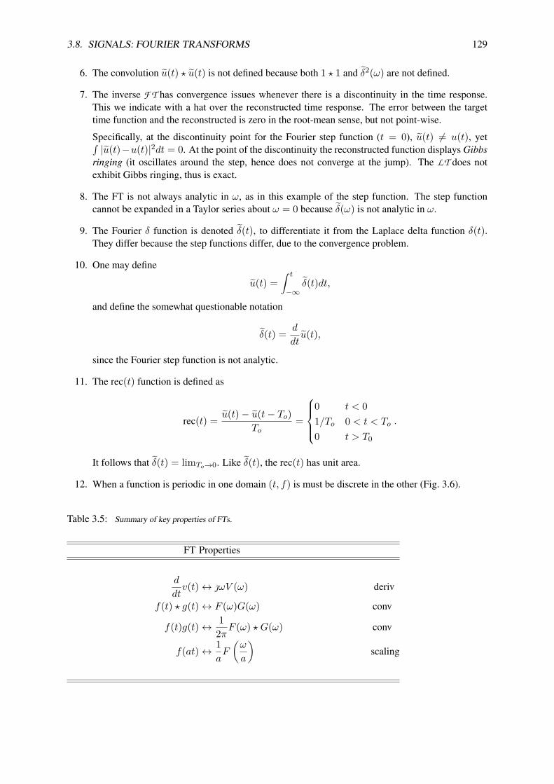
3.8. SIGNALS: FOURIER TRANSFORMS 129
6. The convolution u(t) ? u(t) is not defined because both 1 ? 1 and δ2(ω) are not defined.
7. The inverse F T has convergence issues whenever there is a discontinuity in the time response.This we indicate with a hat over the reconstructed time response. The error between the targettime function and the reconstructed is zero in the root-mean sense, but not point-wise.
Specifically, at the discontinuity point for the Fourier step function (t = 0), u(t) 6= u(t), yet∫|u(t)−u(t)|2dt = 0. At the point of the discontinuity the reconstructed function displays Gibbs
ringing (it oscillates around the step, hence does not converge at the jump). The LT does notexhibit Gibbs ringing, thus is exact.
8. The FT is not always analytic in ω, as in this example of the step function. The step functioncannot be expanded in a Taylor series about ω = 0 because δ(ω) is not analytic in ω.
9. The Fourier δ function is denoted δ(t), to differentiate it from the Laplace delta function δ(t).They differ because the step functions differ, due to the convergence problem.
10. One may define
u(t) =∫ t
−∞δ(t)dt,
and define the somewhat questionable notation
δ(t) = d
dtu(t),
since the Fourier step function is not analytic.
11. The rec(t) function is defined as
rec(t) = u(t)− u(t− To)To
=
0 t < 01/To 0 < t < To
0 t > T0
.
It follows that δ(t) = limTo→0. Like δ(t), the rec(t) has unit area.
12. When a function is periodic in one domain (t, f) is must be discrete in the other (Fig. 3.6).
Table 3.5: Summary of key properties of FTs.
FT Properties
d
dtv(t)↔ ωV (ω) deriv
f(t) ? g(t)↔ F (ω)G(ω) conv
f(t)g(t)↔ 12πF (ω) ? G(ω) conv
f(at)↔ 1aF
(ω
a
)scaling

130 CHAPTER 3. STREAM 2: ALGEBRAIC EQUATIONS
Table 3.6: The general rule is that if a function is discrete in one domain (time or frequency) it is periodic in the other.Abreviations: F T : Fourier Transform; FS: Fourier Series; DTFT: Discrete time Fourier transform; DFT: Discrete Fouriertransform (the FFT is a “fast” DFT);
FREQUENCY \ TIME continuous t discrete tk periodic ((t))Tocontinuous ω F T – –discrete ωk – DFT (FFT) FSperiodic ((ω))Ω – DTFT DFT (FFT)
Periodic signals: Besides these two basic types of time–frequency transforms, there are several vari-ants that depend on the symmetry in time and frequency. For example, when the time signal is sam-pled (discrete in time), the frequency response becomes periodic, leading to the discrete-time Fouriertransform (DTFT). When a time response is periodic, the frequency response is sampled (discrete infrequency), leading to the Fourier series. These two symmetries may be simply characterized as peri-odic in time ⇒ discrete in frequency, and periodic in frequency ⇒ discrete in time. When a functionis discrete both in time and frequency, it is necessarily periodic in time and frequency, leading to thediscrete Fourier transform (DFT). The DFT is typically computed with an algorithm called the fastFourier transform (FFT), which can dramatically speed up the calculation when the data is a power of 2in length.
Causal-periodic signals: An special symmetry occurs given functions that are causal and periodicin frequency. The best example is the z transform, which are causal (one-sided in time) discrete-timesignals. The harmonic series (Eq. 3.28, p. 87) is the z-transform of the discrete-time step function andis thus, due to symmetry, analytic within the RoC in the complex frequency (z) domain.
The double brackets on f((t))To indicate that f(t) is periodic in t with period To, i.e., f(t) =f(t+ kTo) for all k ∈ N. Averaging over one period and dividing by the To gives the average value.
Exercise: Consider the Fourier series scalar (dot) product (Eq. 3.18, p. 105) between “vectors” f((t))Toand e−ωkt
F (ωk) = f((t))To · e−ωkt
≡ 1To
∫ To
0f(t)e−ωktdt,
where ω0 = 2π/To, f(t) has period To, i.e., f(t) = f(t+ nTo) = eωnt with n ∈ N, and ωk = kωo.What is the value of the Fourier series scalar product? Solution: Evaluating the scalar product we
find
eωnt · e−ωkt = 1To
∫ To
0eωnte−ωktdt
= 1To
∫ To
0e2π(n−k)t/Todt =
1 n = k
0 n 6= k.
The two signals (vectors) are orthogonal.
Exercise: Consider the discrete time F T (DTFT) as a scalar (dot) product (Eq. 3.18, between “vec-tors” fn = f(t)|tn and e−ωtn where tn = nTs and Ts = 1/2Fmax is the sample period. Solution: Thescalar product over n ∈ Z is
F ((ω))2π = fn · e−ωtn
≡∞∑
n=−∞fne−ωtn ,
where ω0 = 2π/To and ωk = kωo is periodic (i.e., F (ω) = F (ω + kωo)).

3.9. SYSTEMS: LAPLACE TRANSFORMS 131
3.9 Systems: Laplace transforms
The Laplace transform takes real causal signals f(t)u(t) ∈ R, as a function of real time t ∈ R, that arestrictly zero for negative time (f(t) = 0 for t < 0), and transforms them into complex analytic functions(F (s) ∈ C) of complex frequency s = σ + ω. As for the case of Fourier transform, we use the samenotation: f(t)↔ F (s).
When a signal is zero for negative time f(t < 0) = 0, it is said to be causal, and the resultingtransform F (s) must be complex analytic over significant regions of the s plane. For a function of timeto be causal, time must be real (t ∈ R), since if it were complex, it would lose the order property (thusit could not be causal). It is helpful to emphasize the causal nature of f(t)u(t) to force causality, withthe Heaviside step function u(t).
Any restriction on a function (e.g., real, causal, periodic, positive real part, etc.) is called a symmetryproperty. There are many forms of symmetry (p. 133). The concept of symmetry is very general andwidely used in both mathematics and physics, where it is more generally known as group theory. Asshown in Fig. 3.7 the two most common F T symmetries are continuous and discrete time signal. One-sided periodic transforms also exist, such as the system shown in Fig. 3.3 (p. 78).
Definition of the Laplace transform: The forward and inverse Laplace transforms (see box equa-tions). Here s = σ + jω ∈ C [2πHz] is the complex Laplace frequency in radians and t ∈ R [s] is thetime in seconds. Tables of the more common transforms are provided in Appendix C (p. 269).
Forward and inverse Laplace transforms:
F (s) =∫ ∞
0−f(t)e−stdt f(t) = 1
2π
∫ σo+∞
σo−∞F (s)estds (3.23)
F (s)↔ f(t) f(t)↔ F (s) (3.24)
When dealing with engineering problems it is convenient to separate the signals we use from thesystems that process them. We do this by treating signals, such as a music signal, differently from asystem, such as a filter. In general signals may start and end at any time. The concept of causality hasno mathematical meaning in signal space. Systems, on the other hand, obey very rigid rules (to assurethat they remain physical). These physical restrictions are described in terms of the network postulates,which are discussed on p. 133. There is a question as to why postulates are needed, and which ones arethe best choices. These questions are discussed in his lectures Feynman (1968, 1970a). The originalvideo is also available online in many places, e.g., via youtube.18 19 20 There may be no definitiveanswers to these questions, but having a set of postulates is a useful way of thinking about physics.
Table 3.7: Laplace transforms /LT/s are complementary to the class of Fourier transforms /FT/ due to the fact that the timefunction must be a causal function. All /LT/s are complex analytic in the complex frequency s = σ + ω domain. As anexample, a causal function that is continuous but one-sided in time is the step function u(t), which has the /LT/ u(t) ↔ 1/s.When a function is discrete in time, but one sided, it has a Zeta transform. The discrete-time step function is un = u[n] ↔1/(1− z−n). Abreviations: LT : Laplace Transform; Z-transform: z transforms Series;
FREQUENCY \ TIME continuous t discrete t[k] causal-periodic ((t))Tocontinuous ω LT – –discrete ω[k] – – –periodic |z|eθ – z-Transform –
18https://www.youtube.com/watch?v=JXAfEBbaz_419https://www.youtube.com/watch?v=YaUlqXRPMmY20https://www.youtube.com/watch?v=xnzB_IHGyjg

132 CHAPTER 3. STREAM 2: ALGEBRAIC EQUATIONS
As discussed on p. 179, to invert the LT one must use the Cauchy residue theorem (CT-3), requiringclosure of the contour C at ω→ ±j∞ ∮
C=∫ σ0+j∞
σ0−j∞+∫⊂∞
,
where the path represented by ‘⊂∞’ is a semicircle of infinite radius. For a causal, ‘stable’ (e.g. doesn’t“blow up” in time) signal, all of the poles of F (s) must be inside of the Laplace contour, in the left halfs-plane.
Rig
id w
all
Mass M
Dashpot (resistance) R
Spring compliance CDisplacement x(t)
Force f (t)
Figure 3.10: Three-element mechanical resonant circuit consisting of a spring, mass and dash-pot (e.g., viscous fluid).
Example: Hooke’s law for a spring states that the force f(t) is proportional to the displacement x(t),i.e., f(t) = Kx(t). The formula for a dash-pot is f(t) = Rv(t), and Newton’s famous formula for massis f(t) = d[Mv(t)]/dt, which for a constant M is f(t) = Mdv/dt.
The equation of motion for the mechanical oscillator in Fig. 3.10 is given by Newton’s second law;the sum of the forces must balance to zero
Md2
dt2x(t) +R
d
dtx(t) +Kx(t) = f(t)↔ (Ms2 +Rs+K)X(s) = F (s). (3.25)
These three constants, the mass M , resistance R and stiffness K (∈ R ≥ 0) are real and non-negative.The dynamical variables are the driving force f(t) ↔ F (s), the position of the mass x(t) ↔ X(s) andits velocity v(t)↔ V (s), with v(t) = dx(t)/dt↔ V (s) = sX(s).
Newton’s second law (c1650) is the mechanical equivalent of Kirchhoff’s (c1850) voltage law(KVL), which states that the sum of the voltages around a loop must be zero. The gradient of thevoltage results in a force on a charge (i.e., F = qE). The current may be thought of as the “flow” ofcharge.
Equation 3.25 may be re-expressed in terms of the ratio of sums of impedances, defined as the ratioof the force to velocity, in the Laplace frequency domain.
Example: The divergent series
etu(t) =∞∑0
1n! t
n ↔ 1s− 1
is a valid description of etu(t), with an unstable pole at s = 1. For values of |x− xo| < 1 (x ∈ R), theanalytic function P (x) is said to have a region of convergence (RoC). For cases where the argument iscomplex (s ∈ C), this is called the radius of convergence (RoC). We might call the region |s− so| > 1the region of divergence (RoD), and |s− so| = 0, the singular circle. Typically the underlying functionP (s), defined by the series, has a pole on the singular circle.
There seems to be a conflict with the time response f(t) = eatu(t), which has a divergent series(unstable pole). I’m not sure how to explain this conflict, other than to point out that t ∈ R: thus, theseries expansion of the diverging exponential is real-analytic, not complex analytic. First f(t) has aLaplace transform with a pole at s = 1, in agreement with its unstable nature. Second, every analyticfunction must be single valued. This follows from the fact that each term in Eq. 3.26 is single valued.

3.9. SYSTEMS: LAPLACE TRANSFORMS 133
Third, analytic functions are “smooth” since they may be differentiated an infinite number of times andthe series still converges.
The key idea that every impedance must be complex analytic and ≥ 0 for σ > 0 was first proposedby Otto Brune in his PhD at MIT, supervised by Ernst A. Guillemin, an MIT electrical engineeringprofessor who played an important role in the development of circuit theory and was a student of ArnoldSommerfeld.21 Other MIT advisers were Norbert Wiener and Vannevar Bush. Brune’s primary, butnon-MIT, advisor was W. Cauer, who was trained in 19th century German mathematics, perhaps underSommerfeld (Brune, 1931b).
Summary: While the definitions of the FT (F T ) and LT (LT ) transforms may appear similar, theyare not. The key difference is that the time response of the Laplace transform is causal, leading to acomplex analytic frequency response. The frequency response of the Fourier transform is complex, butnot complex analytic, since the frequency ω is real. Fourier transforms do not have poles.
The concept of symmetry is helpful in understanding the many different types of time-frequencytransforms. Two fundamental types of symmetry are causality (P1) and periodicity.
The Fourier transform F T characterizes the steady-state response while the Laplace transform LTcharacterizes both the transient and steady-state response. Given a causal system responseH(s)↔ h(t)with input x(t), the output is
y(t) = h(t) ? x(t)↔ Y (ω) = H(s)∣∣∣s=ω
X(ω).
3.9.1 System postulates
Solutions of differential equations, such as the wave equation, are conveniently described in terms ofmathematical properties, which we present here in terms of 11 network postulates (see Appendix F,p. 287 for greater detail):
(P1) Causality (non-causal/acausal): Causal systems respond when acted upon. All physical systemsobey causality. An example of a causal system is an integrator, which has a response of a stepfunction. Filters are also examples of causal systems. Signals represent acausal responses. Theydo not have a clear beginning or end, such as the sound of the wind or traffic noise. A causallinear system is typically complex analytic and is naturally represented in the complex s plane viaLaplace transforms. A nonlinear system may be causal, but not complex analytic.
(P2) Linearity (nonlinear): Linear systems obey superposition. Let two signals x(t) and y(t) are theinputs to a linear system, producing outputs x′(t) and y′(t). When the inputs are presented to-gether as ax(t) + by(t) with weights a, b ∈ C, the output will be ax′(t) + by′(t). If either a or bis zero, the corresponding signal is removed from the output.
Nonlinear systems mix the two inputs, thereby producing signals not present in the input. Forexample, if the inputs to a nonlinear system are two sine waves, the output will contain distortioncomponents, having frequencies not present at the input. An example of a nonlinear system is onethat multiplies the two inputs. A second is a diode, which rectifies a signal, letting current flowonly in one direction. Most physical systems have some degree of nonlinear response, but this isnot always desired. Other systems are designed to be nonlinear, such as the diode example.
(P3) Passive (active): An active system has a power source, such as a battery, while a passive system hasno power source. While you may consider a transistor amplifier to be active, it is only so whenconnected to a power source. Brune impedances satisfy the positive-real condition (Eq. 3.36,p. 88).
21It must be noted that University of Illinois Prof. ‘Mac’ Van VanValkenburg was arguably more influential in circuit theoryduring the same period. Mac’s books are certainly more accessible, but perhaps less widely cited.

134 CHAPTER 3. STREAM 2: ALGEBRAIC EQUATIONS
(P4) Real (complex) time response: Typically systems are “real in, real out.” They do not naturallyhave complex responses (real and imaginary parts). While a Fourier transform takes real inputsand produces complex outputs, this is not an example of a complex time response. P4 is a charac-terization of the input signal, not its Fourier transform.
(P5) Time-invariant (time varying): For a system to be a time varying system the output must dependon when the input signal starts or stops. If the output, relative to the input, is independent of thestarting time, then the system is said to be time-invariant.
(P6) Reciprocal (non- or anti-reciprocal): In many ways this is the most difficult propriety to under-stand. It is best characterized by the ABCD matrix (p. 121). If ∆T = 1, the system is said to bereciprocal. If ∆T = −1, it is said to be anti-reciprocal. The impedance matrix is reciprocal whenz12 = z21 and anti-reciprocal when z12 = −z21. Dynamic loudspeakers are anti-reciprocal andmust be modeled by a gyrator, which may be thought of as transformers which swaps the forceand flow variables. For example, the input impedance of a gyrator terminated by an inductor, isa capacitor. This property is best explained by Fig. 3.8 (p. 123). For an extended discussion onreciprocity, see p. 287.
(P7) Reversibility (non-reversible): If swapping the input and output of a system leaves the systeminvariant, it is said to be reversible. When A = D, the system is reversible. Note the distinctionbetween reversible and reciprocal.
(P8) Space-invariant (space-variant): If a system operates independently as a function of where itphysically is in space, then it is space-invariant. When the parameters that characterize the systemdepend on position, it is space-variant.
(P9) Deterministic (random): Given the wave equation, along with the boundary conditions, the sys-tem’s solution may be deterministic, or not, depending on its extent. Consider a radar or sonarwave propagating out into uncharted territory. When the wave hits an object, the reflection can re-turn waves that are not predicted, due to unknown objects. This is an example where the boundarycondition is not known in advance.
(P10) Quasi-static (ka < 1) Quasi-statics follows the Nyquist sampling theorem, for systems that havedimensions that are small compared to the local wavelength (Nyquist, 1924). This assumption failswhen the frequency is raised (the wavelength becomes short). Thus this is also known as the long-wavelength approximation. Quasi-statics is typically stated as ka < 1, where k = 2π/λ = ω/coand a is the smallest dimension of the system. See p. 233 for a detailed discussion of the role ofquasi-statics in acoustic horn wave propagation.
Postulate (P10) is closely related to the Feynman lecture The “underlying unity” of nature whereFeynman asks (Feynman, 1970c, Ch. 12-7): “Why do we need to treat the fields as smooth?” Hisanswer is related to the wavelength of the probing signal relative to the dimensions of the objectbeing probed. This raises the fundamental question: Are Maxwell’s equations a band-limitedapproximation to reality? Today we have no definite answer to this question.
The following quote seems relevant:22
The Lorentz force formula and Maxwell’s equations are two distinct physical laws, yetthe two methods yield the same results.Why the two results coincide was not known. In other words, the flux rule consists oftwo physically different laws in classical theories. Interestingly, this problem was alsoa motivation behind the development of the theory of relativity by Albert Einstein. In1905, Einstein wrote in the opening paragraph of his first paper on relativity theory,“It is known that Maxwell’s electrodynamics – as usually understood at the present
22https://www.sciencedaily.com/releases/2017/09/170926085958.htm

3.10. COMPLEX ANALYTIC MAPPINGS (DOMAIN-COLORING) 135
time – when applied to moving bodies, leads to asymmetries which do not appear to beinherent in the phenomena.” But Einstein’s argument moved away from this problemand formulated special theory of relativity, thus the problem was not solved.Richard Feynman once described this situation in his famous lecture (The FeynmanLectures on Physics, Vol. II, 1964), “we know of no other place in physics where sucha simple and accurate general principle requires for its real understanding an analysisin terms of two different phenomena. Usually such a beautiful generalization is foundto stem from a single deep underlying principle. · · · We have to understand the “rule”as the combined effects of two quite separate phenomena.”
(P11) Periodic ↔ discrete. When a function is discreet in one domain (e.g., time or frequency), it isperiodic in the other (frequency or time).
Summary discussion of the 11 network postulates: Each postulate has at least two categories. Forexample, (P1) is either causal, non-causal or acausal while (P2) is either linear or non-linear. (P6) and(P9) only apply to 2-port algebraic networks (those having an input and an output). The others apply toboth 2– and 1–port networks (e.g., an impedance is a 1-port). An important example of a 2-port is theanti-reciprocal transmission matrix of a dynamic (EM) loudspeaker, p. 287).
Related forms of these postulates may be found in the network theory literature (Van Valkenburg,1964a,b; Ramo et al., 1965). Postulates (P1-P6) were introduced by Carlin and Giordano (1964) and(P7-P9) were added by Kim et al. (2016). While linearity (P2), passivity (P3), realness (P4) and time-invariant (P5) are independent, causality (P1) is a consequence of linearity (P2) and passivity (P3) (Carlinand Giordano, 1964, p. 5).
3.10 Complex analytic mappings (domain-coloring)
One of the most difficult aspects of complex functions of a complex variable is visualizing the mappingsfrom the z = x+ y to w(z) = u+ v planes. For example, w(z) = sin(x) is trivial when z = x+ yis real (i.e., y = 0), because sin(x) is real. Likewise for the case where x = 0,
sin(y) = e−y − ey
2 = − sinh(y)
is pure imaginary. However, the more general case
w(z) = sin(z) ∈ C
is not easily visualized. And when u(x, y) and v(x, y) are less well known functions, w(z) can be evenmore difficult to visualize. For example, ifw(z) = J0(z) then u(x, y), v(x, y) are the real and imaginaryparts of the Bessel function.
A software solution: Fortunately with computer software today, this problem can be solved by addingcolor to the chart. An Octave/Matlab script23 zviz.m has been devised to make the charts shown inFig. 3.11. Such charts are known as domain-coloring.
w = s
σ
-2 -1 0 1 2
jω
2
1
0
-1
-2
w = s-sqrt(j)
σ
-2 -1 0 1 2
jω
2
1
0
-1
-2
Figure 3.11: Left: Domain-colorized map showing the complex map-ping from the s = σ+ω plane to the w(s) = u(σ, ω) + v(σ, ω) plane.This mapping may be visualized by the use of intensity (light/dark) toindicate magnitude, and color (hue) to indicate angle (phase) of the map-ping. Right: This shows the w(s) = s − √ plane, shifted to the rightand up by
√2/2 = 0.707. The white and black lines are the iso-real and
iso-imaginary contours of the mapping.
Rather than plotting u(x, y) andv(x, y) separately, domain-coloring al-lows us to display the entire function onone color chart (i.e., colorized plot). Forthis visualization we see the complex po-lar form of w(s) = |w|e∠w, rather than
23http://jontalle.web.engr.illinois.edu/uploads/298/zviz.zip

136 CHAPTER 3. STREAM 2: ALGEBRAIC EQUATIONS
the 2 × 2 (four-dimensional) Cartesiangraph w(x + y) = u(x, y) + v(x, y).On the left is the reference condition, theidentity mapping (w = s), and on theright the origin has been shifted to theright and up by
√2.
Mathematicians typically use the ab-stract (i.e., non–physical) notation w(z),where w = u+ vı and z = x+ yı. Engi-neers typically work in terms of a physi-cal complex impedance Z(s) = R(s) +X(s), having resistance R(s) and reactance X(s) [ohms], as a function of the complex Laplace radianfrequency s = σ + ω [rad], as used, for example, with the Laplace transform (p. 131).
In Fig. 3.11 we use both notations, with Z(s) = s on the left and w(z) = z − √ on the right,where we show this color code as a 2 × 2 dimensional domain-coloring graph. Intensity (dark to light)represents the magnitude of the function, while hue (color) represents the phase, where (see Fig. 3.11)red is 0, sea-green is 90, blue-green is 135, blue is 180, and violet is −90 (or 270).24
The function w = s = |s|eθ has a dark spot (zero) at s = 0, and becomes brighter away from theorigin. On the right isw(z) = z−√, which shifts the zero (dark spot) to z = √. Thus domain-coloringgives the full 2× 2 complex analytic function mapping w(x, y) = u(x, y) + v(x, y), in colorized polarcoordinates.
Visualizing complex functions: The mapping from z = x + ıy to w(z) = u(x, y) + ıv(x, y)is difficult to visualize because for each point in the domain z, we would like to represent both themagnitude and phase (or real and imaginary parts) of w(z). A good way to visualize these mappings isto use color (hue) to represent the phase and intensity (dark to light) to represent the magnitude.
w = sin(0.5*pi*(s-j))
σ
-2 -1 0 1 2
jω
2
1
0
-1
-2
Figure 3.12: Plot of sin(0.5π(z − i)).
Example: Figure 3.12 shows a colorizedplot of w(z) = sin(π(z − i)/2) result-ing from the Matlab/Octave command zvizsin(pi*(z-i)/2). The abscissa (hori-zontal axis) is the real x axis and the ordinate(vertical axis) is the complex iy axis. Thegraph is offset along the ordinate axis by 1i,since the argument z − i causes a shift ofthe sine function by 1 in the positive imagi-nary direction. The visible zeros of w(z) ap-pear as dark regions at (−2, 1), (0, 1), (2, 1).As a function of x, w(x + 1) oscillates be-tween red (phase is zero degrees), meaningthe function is positive and real, and sea-green (phase is 180), meaning the functionis negative and real.
To use the program use the syntax zviz <function of z> (for example, type zviz z.ˆ2).Note the period between z and ˆ2. This will render a domain-coloring (aka colorized) version of thefunction. Examples you can render with zviz are given in the comments at the top of the zviz.mprogram. A good example for testing is zviz z-sqrt(j), which will show a dark spot (zero) at(1 + 1)/
√2 = 0.707(1 + 1).
Along the vertical axis, the displayed function is either a cosh(y) or sinh(y), depending on the valueof x. The intensity becomes lighter as |w| increases.
24Colors vary depending on both the display medium and the eye.
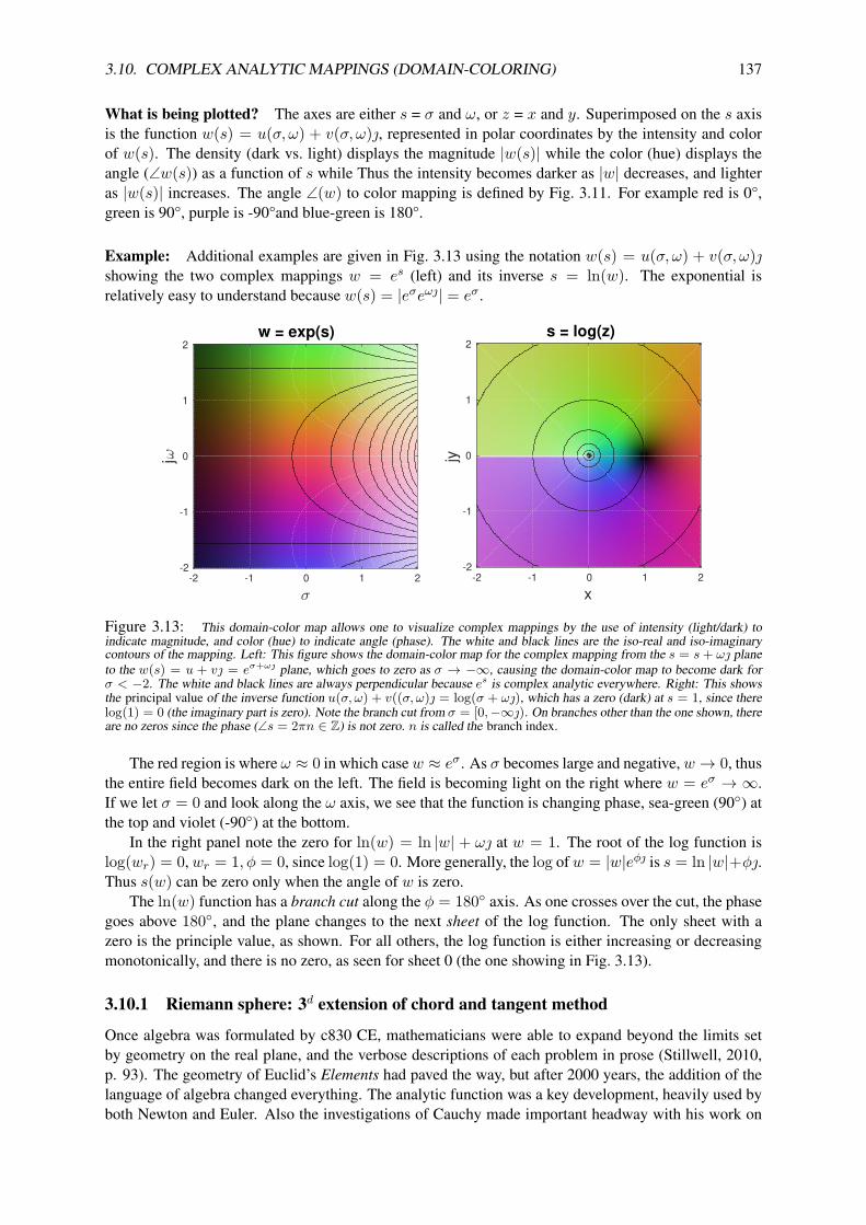
3.10. COMPLEX ANALYTIC MAPPINGS (DOMAIN-COLORING) 137
What is being plotted? The axes are either s = σ and ω, or z = x and y. Superimposed on the s axisis the function w(s) = u(σ, ω) + v(σ, ω), represented in polar coordinates by the intensity and colorof w(s). The density (dark vs. light) displays the magnitude |w(s)| while the color (hue) displays theangle (∠w(s)) as a function of s while Thus the intensity becomes darker as |w| decreases, and lighteras |w(s)| increases. The angle ∠(w) to color mapping is defined by Fig. 3.11. For example red is 0°,green is 90°, purple is -90°and blue-green is 180°.
Example: Additional examples are given in Fig. 3.13 using the notation w(s) = u(σ, ω) + v(σ, ω)showing the two complex mappings w = es (left) and its inverse s = ln(w). The exponential isrelatively easy to understand because w(s) = |eσeω| = eσ.
w = exp(s)
σ
-2 -1 0 1 2
jω
2
1
0
-1
-2
s = log(z)
x-2 -1 0 1 2
jy
2
1
0
-1
-2
Figure 3.13: This domain-color map allows one to visualize complex mappings by the use of intensity (light/dark) toindicate magnitude, and color (hue) to indicate angle (phase). The white and black lines are the iso-real and iso-imaginarycontours of the mapping. Left: This figure shows the domain-color map for the complex mapping from the s = s+ ω planeto the w(s) = u + v = eσ+ω plane, which goes to zero as σ → −∞, causing the domain-color map to become dark forσ < −2. The white and black lines are always perpendicular because es is complex analytic everywhere. Right: This showsthe principal value of the inverse function u(σ, ω) + v((σ, ω) = log(σ + ω), which has a zero (dark) at s = 1, since therelog(1) = 0 (the imaginary part is zero). Note the branch cut from σ = [0,−∞). On branches other than the one shown, thereare no zeros since the phase (∠s = 2πn ∈ Z) is not zero. n is called the branch index.
The red region is where ω ≈ 0 in which casew ≈ eσ. As σ becomes large and negative, w → 0, thusthe entire field becomes dark on the left. The field is becoming light on the right where w = eσ → ∞.If we let σ = 0 and look along the ω axis, we see that the function is changing phase, sea-green (90) atthe top and violet (-90) at the bottom.
In the right panel note the zero for ln(w) = ln |w| + ω at w = 1. The root of the log function islog(wr) = 0,wr = 1, φ = 0, since log(1) = 0. More generally, the log ofw = |w|eφ is s = ln |w|+φ.Thus s(w) can be zero only when the angle of w is zero.
The ln(w) function has a branch cut along the φ = 180 axis. As one crosses over the cut, the phasegoes above 180, and the plane changes to the next sheet of the log function. The only sheet with azero is the principle value, as shown. For all others, the log function is either increasing or decreasingmonotonically, and there is no zero, as seen for sheet 0 (the one showing in Fig. 3.13).
3.10.1 Riemann sphere: 3d extension of chord and tangent method
Once algebra was formulated by c830 CE, mathematicians were able to expand beyond the limits setby geometry on the real plane, and the verbose descriptions of each problem in prose (Stillwell, 2010,p. 93). The geometry of Euclid’s Elements had paved the way, but after 2000 years, the addition of thelanguage of algebra changed everything. The analytic function was a key development, heavily used byboth Newton and Euler. Also the investigations of Cauchy made important headway with his work on

138 CHAPTER 3. STREAM 2: ALGEBRAIC EQUATIONS
complex variables. Of special note was integration and differentiation in the complex plane of complexanalytic functions, which is the topic of stream 3.
It was Riemann, working with Gauss in the final years of Gauss’s life, who made the breakthrough,with the concept of the extended complex plane.25 This concept was based on the composition of a linewith the sphere, similar to the derivation of Euclid’s formula for Pythagorean triplets (p. 56). Whilethe importance of the extended complex plane was unforeseen, it changed analytic mathematics forever,along with the physics it supported. It unified and thus simplified many important integrals, to theextreme. The basic idea is captured by the fundamental theorem of complex integral calculus (Table 4.1,p. 149).
Figure 3.14: The left panel shows how the real line may be composed with the circle. Each real x value maps to acorresponding point x′ on the unit circle. The point x → ∞ maps to the north pole N . This simple idea may be extendedwith the composition of the complex plane with the unit sphere, thus mapping the plane onto the sphere. As with the circle,the point on the complex plane z → ∞ maps onto the north pole N . This construction is important because while the planeis open (does not include z →∞), the sphere is analytic at the north pole. Thus the sphere defines the closed extended plane.Figure adapted from Stillwell (2010, pp. 299-300).
The idea is outlined in Fig. 3.14. On the left is a circle and a line. The difference between this caseand the derivation of the Pythagorean triplets is that the line starts at the north pole, and ends on thereal x ∈ R axis at point x. At point x′, the line cuts through the circle. Thus the mapping from x tox′ takes every point on R to a point on the circle. For example, the point x = 0 maps to the south pole(not indicated). To express x′ in terms of x one must compose the line and the circle, similar to thecomposition used in the derivation of Euclid’s formula (p. 56). The points on the circle, indicated hereby x′, require a traditional polar coordinate system, having a unit radius and an angle defined betweenthe radius and a vertical line passing through the north pole. When x → ∞ the point x′ → N , knownas the point at infinity. But this idea goes much further, as shown on the right half of Fig. 3.14.
Here the real tangent line is replaced by a tangent complex plane z ∈ C, and the complex puncturepoint z′ ∈ C, in this case on the complex sphere, called the extended complex plane. This is a naturalextension of the chord/tangent method on the left, but with significant consequences. The main differ-ence between the complex plane z and the extended complex plane, other than the coordinate system, iswhat happens at the north pole. The point at |z| =∞ is not defined on the plane, whereas on the sphere,the point at the north pole is simply another point, like every other point on the sphere.
Open vs. closed sets: Mathematically the plane is said to be an open set, since the limit z →∞ is notdefined, whereas on the sphere, the point z′ is a member of a closed set, since the north pole is defined.The distinction between an open and closed set is important, because the closed set allows the functionto be complex analytic at the north pole, which it cannot be on the plane (since the point at infinity isnot defined).
The z plane may be replaced with another plane, say the w = F (z) ∈ C plane, where w is somefunction F of z ∈ C. For the moment we shall limit ourselves to complex analytic functions of z, namelyw = F (z) = u(x, y) + v(x, y) =
∑∞n=0 cnz
n.25“Gauss did lecture to Riemann but he was only giving elementary courses and there is no evidence that at this time he
recognized Riemann’s genius.” Then “In 1849 he [Riemann] returned to Gottingen and his Ph.D. thesis, supervised by Gauss,was submitted in 1851.” http://www-groups.dcs.st-and.ac.uk/˜history/Biographies/Riemann.html

3.10. COMPLEX ANALYTIC MAPPINGS (DOMAIN-COLORING) 139
In summary, given a point z = x+ y on the open complex plane, we map it to w = F (z) ∈ C, thecomplex w = u + v plane, and from there to the closed extended complex plane w′(z). The point ofdoing this is that it allows us to allow the function w′(z) to be analytic at the north pole, meaning it canhave a convergent Taylor series at the point at infinity z →∞. Since we have not yet defined dw(z)/dz,the concept of a complex Taylor series remains undefined.
3.10.2 Bilinear transformation
In mathematics the bilinear transformation has special importance because it is linear in its action onboth the input and output variables. Since we are engineers we shall stick with the engineering termi-nology. But if you wish to read about this on the internet, be sure to also search for the mathematicalterm, Mobius transformation.
When a point on the complex plane z = x+ y is composed with the bilinear transform (a, b, c, d ∈C), the result is w(z) = u(x, y) + v(x, y) (this is related to the Mobius transform, p. 29)
w = az + b
cz + d. (3.26)
The transformation from z → w is a cascade of four independent compositions:
1. translation (w = z + b: a = 1, b ∈ C, c = 0, d = 1),
2. scaling (w = |a|z: a ∈ R, b = 0, c = 0, d = 1),
3. rotation (w = a|a|z: a ∈ C, b = 0, c = 0, d = |a|) and
4. inversion (w = 1z : a = 0, b = 1, c = 1, d = 0).
Each of these transformations is a special case of Eq. 3.26, with the inversion the most complicated.I highly recommend a video showing the effect of the bilinear (Mobius) transformation on the plane(Arnold, Douglas and Rogness, Jonathan , 2019).26
The bilinear transformation is the most general way to move the expansion point in a complexanalytic expansion. For example, starting from the harmonic series, the bilinear transform gives
11− w = 1
1− az+bcz+d
= cz + d
(c− a)z + (d− b) .
The RoC is transformed from |w| < 1 to |(az − b)/(cz − d)| < 1. An interesting application might bein moving the expansion point until it is on top of the nearest pole, so that the RoC goes to zero. Thismight be a useful way of finding a pole, for example.
When the extended plane (Riemann sphere) is analytic at z =∞, one may take the derivatives there,defining the Taylor series with the expansion point at∞. When the bilinear transformation rotates theRiemann sphere, the point at infinity is translated to a finite point on the complex plane, revealing theanalytic nature at infinity. A second way to transform the point at infinity is by the bilinear transformationζ = 1/z, mapping a zero (or pole) at z = ∞ to a pole (or zero) at ζ = 0. Thus this construction of theRiemann sphere and the Mbious (bilinear) transformation allows us to understand the point at infinity,and treat it like any other point. If you felt that you never understood the meaning of the point at ∞(likely), this should help.
26https://www.youtube.com/watch?v=0z1fIsUNhO4

140 CHAPTER 3. STREAM 2: ALGEBRAIC EQUATIONS
3.11 Exercises AE-3
Topic of this homework:
Visualizing complex functions; Bilinear/Mobius transform; Riemann sphere.
Algebra
Problem # 1: Fundamental theorem of algebra (FTA)
–Q 1.1: State the fundamental theorem of algebra (FTA).
Problem # 2: Order and complex numbers:One can always say that 3<4, namely that real numbers have order. One way to view this is to take thedifference, and compare to zero, as in 4− 3 > 0. Here, we will explore how complex variables may beordered. Define the complex variable z = x+ iy ∈ C.
–Q 2.1: Explain the meaning of |z1| > |z2|.
–Q 2.2: If x1, x2 ∈ R (are real numbers), define the meaning of x1 > x2.Hint: Take the difference.
–Q 2.3: Explain the meaning of z1 > z2.
–Q 2.4: If time were complex how might the world be different?(not graded)
Problem # 3: It is sometimes necessary to consider a function w(z) = u + iv in terms of thereal functions, u(x, y) and v(x, y) (e.g. separate the real and imaginary parts). Similarly, wecan consider the inverse z(w) = x+ iy where x(u, v) and y(u, v) are real functions.
–Q 3.1: Find u(x, y) and v(x, y) for w(z) = 1/z.
Problem # 4: Find u(x, y) and v(x, y) for w(z) = cz with complex constant c ∈ C for thefollowing cases:
–Q 4.1: c = e
–Q 4.2: c = 1 (recall that 1 = ei2πk for k = 0, 1, 2, . . .)
–Q 4.3: c = . Hint: = eπ/2.
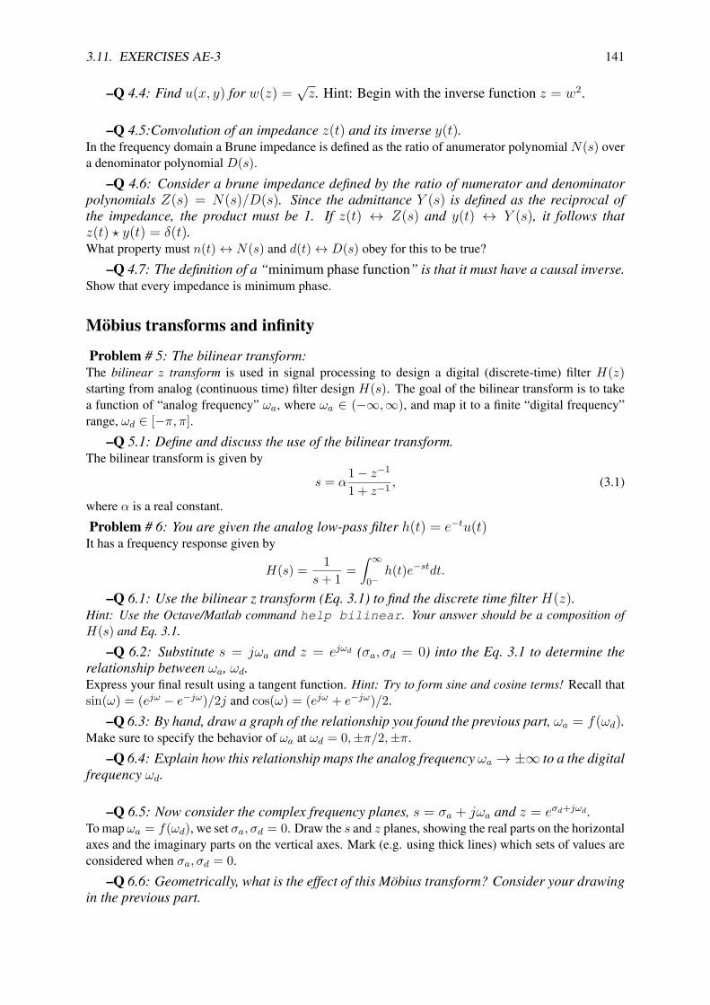
3.11. EXERCISES AE-3 141
–Q 4.4: Find u(x, y) for w(z) =√z. Hint: Begin with the inverse function z = w2.
–Q 4.5:Convolution of an impedance z(t) and its inverse y(t).In the frequency domain a Brune impedance is defined as the ratio of anumerator polynomial N(s) overa denominator polynomial D(s).
–Q 4.6: Consider a brune impedance defined by the ratio of numerator and denominatorpolynomials Z(s) = N(s)/D(s). Since the admittance Y (s) is defined as the reciprocal ofthe impedance, the product must be 1. If z(t) ↔ Z(s) and y(t) ↔ Y (s), it follows thatz(t) ? y(t) = δ(t).What property must n(t)↔ N(s) and d(t)↔ D(s) obey for this to be true?
–Q 4.7: The definition of a “minimum phase function” is that it must have a causal inverse.Show that every impedance is minimum phase.
Mobius transforms and infinity
Problem # 5: The bilinear transform:The bilinear z transform is used in signal processing to design a digital (discrete-time) filter H(z)starting from analog (continuous time) filter design H(s). The goal of the bilinear transform is to takea function of “analog frequency” ωa, where ωa ∈ (−∞,∞), and map it to a finite “digital frequency”range, ωd ∈ [−π, π].
–Q 5.1: Define and discuss the use of the bilinear transform.The bilinear transform is given by
s = α1− z−1
1 + z−1 , (3.1)
where α is a real constant.
Problem # 6: You are given the analog low-pass filter h(t) = e−tu(t)It has a frequency response given by
H(s) = 1s+ 1 =
∫ ∞0−
h(t)e−stdt.
–Q 6.1: Use the bilinear z transform (Eq. 3.1) to find the discrete time filter H(z).Hint: Use the Octave/Matlab command help bilinear. Your answer should be a composition ofH(s) and Eq. 3.1.
–Q 6.2: Substitute s = jωa and z = ejωd (σa, σd = 0) into the Eq. 3.1 to determine therelationship between ωa, ωd.Express your final result using a tangent function. Hint: Try to form sine and cosine terms! Recall thatsin(ω) = (ejω − e−jω)/2j and cos(ω) = (ejω + e−jω)/2.
–Q 6.3: By hand, draw a graph of the relationship you found the previous part, ωa = f(ωd).Make sure to specify the behavior of ωa at ωd = 0,±π/2,±π.
–Q 6.4: Explain how this relationship maps the analog frequency ωa → ±∞ to a the digitalfrequency ωd.
–Q 6.5: Now consider the complex frequency planes, s = σa + jωa and z = eσd+jωd .To map ωa = f(ωd), we set σa, σd = 0. Draw the s and z planes, showing the real parts on the horizontalaxes and the imaginary parts on the vertical axes. Mark (e.g. using thick lines) which sets of values areconsidered when σa, σd = 0.
–Q 6.6: Geometrically, what is the effect of this Mobius transform? Consider your drawingin the previous part.

142 CHAPTER 3. STREAM 2: ALGEBRAIC EQUATIONS
Probability
Many things in life follow rules we don’t understand, thus are unpredictable, yet have structure due tosome underlying poorly understood physics (e.g., quantum mechanics). Unlike mathematicians, engi-neers are taught to deal with uncertainty, in terms of random processes, using probability theory. Formany this starts out as a large set of boreing incomprehensible definitions, but once you begin to under-stand it, becomes interesting mathematics. It needs to be in your skin. If you don’t have an intuition forit, either keep working on it, or else find another job. Don’t memorize a bunch of formulae, because thatwon’t work over the long run.
Some view probability as combinatorics. This is wrong. It is much more than that. From myauditory vew of speech in noise, probability is about the signal processing of noise and signals (i.e., notcombinatorics). For insight read Hamming (2004).
Definitions:
1. An event is the term to describe an unpredictable outcome (Papoulis and Pillai, 2002).
Example: Measuring the temperature T (x, t) ∈ R with x ∈ R3 at time t [s] is an event.
Example: Measuring the temperature every hour gives 24 events per day [degrees/hr].
Example: The single toss of a coin, resulting in H,T, is an event.
–Q 6.7: What are the units of a coin toss?
–Q 6.8: What are the units of H,T?
2. A trial is N events.
3. An experiment M,N is defined as M trials of N events.
4. Number of events: One must always keep track of the number of events so that one can computethe mean (i.e., average) and the uncertainty of an observable outcome.
5. The mean of many trials is the average.
6. A random variable X is defined as the outcome from an experiment. A random variable rarelyhas stated units.
Example: Flipping a coin N = 8 times defines the number of trials.
–Q 6.9: Give the units of coin flips?
X ≡ H,H,H, T,H, T, T, T.
–Q 6.10: How do you give mean to something that doesn’t have units?
–Q 6.11: What is the mean and standard deviation of the coin toss?
7. The Expected value is the mean of N events.

3.11. EXERCISES AE-3 143
–Q 6.12: What is the difference between the mean, expected value and the average?
–Q 6.13: How to assign mean outcomes H,T using numbers.
8. Note: It is critically important to keep track of the number of events (N = 8 in the above example)because N is more important than the actual measured sequence.
9. Note: It is helpful to think of N as the independent variable and X as the dependent variable. Forexample, think ofX(N) rather thanN(X). Concentrate on the fixedN , not the random sequence.
Example: To form a trial by fliping a coin N = 10 times. We form an experiment by M repeatedtrials (M = 1000).
Problem # 7: Basic terminology of experiments
–Q 7.1: What is the mean of a trial, and what is the average over all trials?
–Q 7.2: What is the “expected value” of a random variable X?
–Q 7.3: What is the “standard deviation” about the “mean”?
–Q 7.4: What is the definition of “information” of a random variable?
–Q 7.5: What is the “entropy” of a random variable?
–Q 7.6: What is the “sampling noise” of a random variable?
–Q 7.7:How to you combine events? Hint: if the event is the flip of a biased coin, the evenis H = p, T = 1− p, so the event is p, 1− p.To solve the problem, you must find the probabilities of two independent events.
–Q 7.8:What does the term “independent” mean in this context? Give an example.
–Q 7.9: Define the term “odds”.

144 CHAPTER 3. STREAM 2: ALGEBRAIC EQUATIONS

Chapter 4
Stream 3a: Scalar (Ordinary) DifferentialEquations
Stream 3 is ∞, a concept which typically means unbounded (immeasurably large), but in the case ofcalculus, ∞ means infinitesimal (immeasurably small), since taking a limit requires small numbers.Taking a limit means you may never reach the target, a concept that the Greeks called Zeno’s paradox(Stillwell, 2010, p. 76).
When speaking of the class of ordinary (versus vector) differential equations, the term scalar ispreferable, since the term “ordinary” is vague, if not a meaningless label. There is a special subset offundamental theorems for scalar calculus, all of which are about integration, as summarized in Table 4.1(p. 149), starting with Leibniz’s theorem. These will be discussed below, and more extensively on pages147, 145) and 145.
Following the integral theorems on scalar calculus are those on vector calculus, without which therecan be no understanding of Maxwell’s equations. Of these, the fundamental theorem of complex calculus(aka, Helmholtz decomposition), Gauss’s law and Stokes’s theorem form three cornerstones of modernvector field analysis. These theorems allow one to connect the differential (point) and macroscopic(integral) relationships. For example, Maxwell’s equations may be written as either vector differentialequations, as shown by Heaviside (along with Gibbs and Hertz), or in integral form. It is helpful toplace these two forms side-by-side, to fully appreciate their significance. To understand the differential(microscopic) view, one must understand the integral (macroscopic) view. These are presented in Fig. 5.5(p. 221) and Fig. 5.6 (p. 222).
4.1 The beginning of modern mathematics
As outlined in Fig. 1.2 (p. 17), mathematics as we know it today, began in the 16th to 18th centuries,arguably starting with Galileo, Descartes, Fermat, Newton, the Bernoulli family, and most importantly,Euler. Galileo was formidable, due to his fame, fortune, and his “successful” stance against the power-ful Catholic establishment. His creativity in scientific circles was certainly well known due to his manyskills and accomplishments. Descartes and Fermat were at the forefront of merging algebra and geom-etry. While Fermat kept meticulous notebooks, he did not publish, and tended to be secretive. ThusDescartes’s contributions were more widely acknowledged, but not necessarily deeper.
Regarding the development of calculus, much was yet to be developed by Newton and Leibniz,using term-by-term integration of functions based on Taylor series representation. This was a powerfultechnique, but as stated earlier, incomplete because the Taylor series can only represent single-valuedfunctions, within the RoC. But more importantly, Newton (and others) failed to recognize (i.e., rejected)the powerful generalization to complex analytic functions. The first major breakthrough was Newton’spublication of Principia (1687), and the second was Riemann (1851), advised by Gauss.
Following Newton’s lead, the secretive and introverted behavior of the typical mathematician dra-matically changed with the Bernoulli family (Fig. 3.1, p. 70). The oldest brother Jacob taught his much
145

146 CHAPTER 4. STREAM 3A: SCALAR CALCULUS
younger brother Johann, who then taught his son Daniel. But Johann’s star pupil was Euler. Euler firstmastered all the tools and then published, with a prolificacy previously unknown.
Euler and the circular functions: The first major task was to understand the family of analytic cir-cular functions, ex, sin(x), cos(x), and log(x), a task begun by the Bernoulli family, but mastered byEuler. Euler sought relations between these many functions, some of which may not be thought of asbeing related, such as the log and sin functions. The connection that may “easily” be made is throughtheir complex Taylor series representation (Eq. 3.27, p. 85). By the manipulation of the analytic seriesrepresentations, the relationship between ex, and the sin(x) and cos(x), was precisely captured with therelation
ejω = cos(ω) + sin(ω), (4.1)
and its analytic inverse (Greenberg, 1988, p. 1135)
tan−1(z) = 12 ln
(1− z1+ z
). (4.2)
The phase is φ(ω) = ∠z, from which one may compute the group delay
τg(ω) = − 12π
∂φ(ω)∂ω
.
Exercise: Starting from Eq. 4.1, derive Eq. 4.2. Solution: Solution: Let z(ω) = tanω, then
z(ω) = sinωcosω = tan(ω) = −e
ω − e−ω
eω + e−ω= −e
2ω − 1e2ω + 1 . (4.3)
Solving this for e2ω gives
e2ω = 1 + z
1− z . (4.4)
Taking the square root results in the analytic relationship between eω and tanω
eω = ±√
1 + z
1− z .
Taking the log, and using the definition of ω(z) = tan−1(z), we obtain Eq. 4.2.These equations are the basis of transmission lines (TL) and the Smith chart. Here z(ω) is the TL’s
input impedance and Eq. 4.4 is the reflectance.
While many high school students memorize Euler’s relation, it seems unlikely they appreciate theutility of complex analytic functions (Eq. 3.39, p. 91).
History of complex analytic functions: Newton (c1650) famously ignored imaginary numbers, andcalled them imaginary in a disparaging (pejorative) way. Given Newton’s prominence, his view certainlymust have keenly attenuated interest in complex algebra, even though it had been previously describedby Bombelli in 1526, likely based on his serendipitous finding of Diophantus’s book Arithmetic in theVatican library.
Euler derived his relationships using real power series (i.e., real analytic functions). While Eulerwas fluent with =
√−1, he did not consider functions to be complex analytic. That concept was first
explored by Cauchy almost a century later. The missing link to the concept of complex analytic is thedefinition of the derivative with respect to the complex argument
F ′(s) = dF (s)ds
, (4.5)

4.2. FUNDAMENTAL THEOREMS OF SCALAR CALCULUS 147
s = atan(z)
x-2 -1 0 1 2
jy
2
1
0
-1
-2
s = (i/2)*log((1-i*z)./(1+i*z))
x-2 -1 0 1 2
jy
2
1
0
-1
-2
Figure 4.1: Colorized plots of ω(z) = tan−1(z) and ω(z) = i2 ln(1− iz)/(1 + iz), verifying they are the same complex
analytic function.
where s = σ + ω, without which the complex analytic Taylor coefficients may not be defined.Euler did not appreciate the role of complex analytic functions because these were first discovered
well after his death (1785) by Augustin-Louis Cauchy (1789–1857), and extended by Riemann in 1851(p. 122).
4.2 Fundamental theorems of scalar calculus
History of the fundamental theorem of scalar calculus: It some sense, the story of calculus beginswith the fundamental theorem of calculus (FTC), also known generically as Leibniz’s formula. Thesimplest integral is the length of a line L =
∫ L0 dx. If we label a point on a line as x = 0 and wish
to measure the distance to any other point x, we form the line integral between the two points. If theline is straight, this integral is simply the Euclidean length given by the difference between the two ends(Eq. 3.5.1, p. 105).
If F (χ) ∈ R describes a height above the line χ ∈ R, then f(x)
f(x)− f(0) =∫ x
x=0F (χ)dχ (4.6)
may be viewed as the anti-derivative of F (χ). Here χ is a dummy variable of integration. Thus the areaunder F (χ) only depends on the difference of the area evaluated at the end points. It makes intuitivesense to view f(x) as the anti-derivative of F (χ).
This property of the area as an integral over an interval, only depending on the end points, has impor-tant consequences in physics in terms of conservation of energy, allowing for important generalizations.For example, as long as χ ∈ R, one may let F (χ) ∈ C with no loss of generality, due to the linearpropriety (P1, p. 133) of the integral.
If f(x) is analytic (Eq. 3.26, p. 85), then
F (x) = d
dxf(x) (4.7)
is an exact real differential. It follows that F (x) is analytic. This is known as the fundamental theoremof (real) calculus (FTC). Thus Eq. 4.7 may be viewed as an exact real differential. This is easily shownby evaluating
d
dxf(x) = lim
δ→0
f(x+ δ)− f(x)δ
= F (x),
148 CHAPTER 4. STREAM 3A: SCALAR CALCULUS
starting from the anti-derivative Eq. 4.6. If f(x) is not analytic then the limit may not exist, so this is anecessary condition.
There are many important variations on this very basic theorem (i.e., p. 145). For example, the limitscould depend on time. Also when taking Fourier transforms, the integrand depends on both time t ∈ Rand frequency ω ∈ R via a complex exponential “kernel” function e±ωt ∈ C, which is analytic in botht and ω.
4.2.1 The fundamental theorems of complex calculus:
The fundamental theorem of complex calculus (FTCC) states (Greenberg, 1988, p. 1197) that for anycomplex analytic function F (s) ∈ C with s = σ + ω ∈ C,
f(s)− f(so) =∫ s
soF (ζ)dζ. (4.8)
Equations 4.6 and 4.8 differ because the path of the integral is complex. Thus the line integral is overs ∈ C rather than a real integral over χ ∈ R. The fundamental theorem of complex calculus (FTCC)states that the integral only depends on the end points, since
F (s) = d
dsf(s). (4.9)
Comparing exact differentials Eq. 4.5 (FTCC) and Eq. 4.7 (FTC), we see that f(s) ∈ C must be complexanalytic, and have a Taylor series in powers in s ∈ C. It follows that F (s) is also complex analytic.
Complex analytic functions: The definition of a complex analytic function F (s) of s ∈ C is that thefunction may be expanded in a Taylor series (Eq. 3.38, p. 91) about an expansion point so ∈ C. Thisdefinition follows the same logic as the FTC. Thus we need a definition for the coefficients cn ∈ C,which most naturally follow from Taylor’s formula
cn = 1n!
dn
dsnF (s)
∣∣∣∣s=so
. (4.10)
The requirement that F (s) have a Taylor series naturally follows by taking derivatives with respect to sat so. The problem is that both integration and differentiation of functions of complex Laplace frequencys = σ + ω have not yet been defined.
Thus the question is: What does it mean to take the derivative of a function F (s) ∈ C, s = σ+ω ∈C, with respect to s, where s defines a plane rather than a real line? We learned how to form thederivative on the real line. Can the same derivative concept be extended to the complex plane?
The answer is affirmative. The question may be resolved by applying the rules of the real derivativewhen defining the derivative in the complex plane. However, for the complex case, there is an issueregarding direction. Given any analytic function F (s), is the partial derivative with respect to σ differentfrom the partial derivative with respect to ω? For complex analytic functions, the FTCC states that theintegral is independent of the path in the s plane. Based on the chain rule, the derivative must also beindependent of direction at so. This directly follows from the FTCC. If the integral of a function of acomplex variable is to be independent of the path, the derivative of a function with respect to a complexvariable must be independent of the direction. This follows from Taylor’s formula, Eq. 4.10, for thecoefficients of the complex analytic formula.
The Cauchy-Riemann conditions: The FTC defines the area as an integral over a real differential(dx ∈ R), while the FTCC relates an integral over a complex function F (s) ∈ C, along a complexinterval (i.e., path) (ds ∈ C). For the FTC the area under the curve only depends on the end points of theanti-derivative f(x). But what is the meaning of an “area” along a complex path? The Cauchy-Riemannconditions provide the answer.

4.2. FUNDAMENTAL THEOREMS OF SCALAR CALCULUS 149
Table 4.1: Summary of the fundamental theorems of integral calculus, each of which deals with integration. There are atleast two main theorems related to scalar calculus, and three more for vector calculus.
Name Mapping p. DescriptionLeibniz (FTC) R1 → R0 147 Area under a real curveCauchy (FTCC) C1 → R0 147 Area under a complex curveCauchy’s theorem C1 → C0 167 Close integral over analytic region is zeroCauchy’s integral formula C1 → C0 167 Fundamental theorem of complex integral calculusresidue theorem C1 → C0 167 Residue integrationHelmholtz’s theorem
4.2.2 Cauchy-Riemann conditions
For the integral of Z(s) = R(σ, ω) + X(σ, ω) to be independent of the path, the derivative of Z(s)must be independent of the direction of the derivative. As we show next, this leads to a pair of equationsknown as the Cauchy-Riemann conditions. This is an important generalization of Eq. 1.1 (p. 15), whichgoes from real integration (x ∈ R) to complex integration (s ∈ C) based on lengths, thus on area.
To defined
dsZ(s) = d
ds[R(σ, ω) + X(σ, ω)] ,
take partial derivatives of Z(s) with respect to σ and ω, and equate them:
∂Z
∂σ= ∂R
∂σ+
∂X
∂σ≡ ∂Z
∂ω= ∂R
∂ω+
∂X
∂ω.
This says that a horizontal derivative, with respect to σ, is equivalent to a vertical derivative, with respectto ω. Taking the real and imaginary parts gives the two equations
CR-1:∂R(σ, ω)∂σ
= ∂X(σ, ω)∂ω
and CR-2:∂R(σ, ω)∂ω
= −∂X(σ, ω)
∂σ, (4.11)
known as the Cauchy-Riemann (CR) conditions. The cancels in CR-1, but introduces a 2 = −1 inCR-2. They may also be written in polar coordinates (s = reθ) as
∂R
∂r= 1r
∂X
∂θand
∂X
∂r= −1
r
∂R
∂θ.
If you are wondering what would happen if we took a derivative at 45 degrees, then we only need tomultiply the function by eπ/4. But doing so will not change the derivative. Thus we may take thederivative in any direction by multiplying by eθ, and the CR conditions will not change.
The CR conditions are necessary conditions that the integral of Z(s), and thus its derivative, beindependent of the path, expressed in terms of conditions on the real and imaginary parts of Z. This is avery strong condition on Z(s), which follows assuming that Z(s) may be written as a Taylor series in s:
Z(s) = Zo + Z1s+ 12Z2s
2 + · · · , (4.12)
where Zn ∈ C are complex constants given by the Taylor series formula (Eq. 4.10, p. 148). As withthe real Taylor series, there is the convergence condition, that |s| < 1, called the radius of convergence(RoC). This is an important generalization of the region of convergence (R0C) for real s = x.
Every function that may be expressed as a Taylor series in s − so about point so ∈ C is said tobe complex analytic at so. This series, which must be single valued, is said to converge within a ra-dius of convergence (RoC). This highly restrictive condition has significant physical consequences. For

150 CHAPTER 4. STREAM 3A: SCALAR CALCULUS
example, every impedance function Z(s) obeys the CR conditions over large regions of the s plane, in-cluding the entire right half-plane (RHP) (σ > 0). This condition is summarized by the Brune condition<Z(σ > 0) ≥ 0, or alternatively ∠Z(s) < ∠s (Eq. 4.15, p. 159).
When the CR condition is generalized to volume integrals, it is called Green’s theorem, the solutionof boundary value problems in engineering and physics (Kusse and Westwig, 2010). For example, p. 145and p. 187 depend heavily on these concepts.
We may merge these equations into a pair of second-order equations by taking a second round ofpartials. Specifically, eliminating the real part R(σ, ω) of Eq. 4.11 gives
∂2R(σ, ω)∂σ∂ω
= ∂2X(σ, ω)∂2ω
= −∂2X(σ, ω)∂2σ
, (4.13)
which may be compactly written as∇2X(σ, ω) = 0. Eliminating the imaginary part gives
∂2X(σ, ω)∂ω∂σ
= ∂2R(σ, ω)∂2σ
= −∂2R(σ, ω)∂2ω
, (4.14)
which may be written as∇2R(σ, ω) = 0.In summary, for a function Z(s) to be complex analytic, the derivative dZ/ds must be independent
of direction (path), which requires that the real and imaginary parts of the function obey Laplace’sequation, i.e.,
CR-3: ∇2R(σ, ω) = 0 and CR-4: ∇2X(σ, ω) = 0. (4.15)
The CR equations are easier to work with because they are first-order, but the physical intuition is bestunderstood by noting two facts (1) the derivative of a complex analytic function is independent of itsdirection, and (2) the real and imaginary parts of the function both obey Laplace’s equation. Suchrelationships are known as harmonic functions.1
As we shall see in the next few sections, complex analytic functions must be smooth since everyanalytic function may be differentiated an infinite number of times, within the RoC. The magnitudemust attain its maximum and minimum on the boundary. For example, when you stretch a rubber sheetover a jagged frame, the height of the rubber sheet obeys Laplace’s equation. Nowhere can the height ofthe sheet rise above or below its value at the boundary.
Harmonic functions define conservative fields, which means that energy (like a volume or area) isconserved. The work done in moving a mass from a to b in such a field is conserved. If you return themass from b back to a, the energy is retrieved, and zero net work has been done.
1When the function is the ratio of two polynomials, as in the cases of the Brune impedance, they are also related to Mobiustransformations, also know as bi-harmonic operators.

4.3. EXERCISES DE-1 151
4.3 Exercises DE-1
Topic of this homework:
Complex numbers and functions (ordering and algebra); Complex power series; Fundamental theoremof calculus (real and complex); Cauchy-Riemann conditions; Multivalued functions (branch cuts andRiemann sheets)
Complex Power Series
Problem # 1: In each case derive (e.g. using Taylor’s formula) the power series of w(s) abouts = 0 and state the ROC of your series. If the power series doesn’t exist, state why! Hint: Insome cases, you can derive the series by relating the function to another function for which youalready know the power series at s = 0.
–Q 1.1: 1/(1− s)
–Q 1.2: 1/(1− s2)
–Q 1.3: 1/(1− s)2
–Q 1.4: 1/(1 + s2). Hint: This series will be very ugly to derive if you try to take thederivatives dn
dsn[1/(1 + s2)]. Using the results of our previous homework, you should represent
this function as w(s) = −0.5i/(s− i) + 0.5i/(s+ i).
–Q 1.5: 1/s
–Q 1.6: 1/(1− |s|2)
Problem # 2: Consider the function w(s) = 1/s
–Q 2.1: Expand this function as a power series about s = 1. Hint: Let 1/s = 1/(1−1+s) =1/(1− (1− s)).
–Q 2.2: What is the ROC?
–Q 2.3: Expand w(s) = 1/s as a power series in s−1 = 1/s about s−1 = 1.
152 CHAPTER 4. STREAM 3A: SCALAR CALCULUS
–Q 2.4: What is the ROC?
–Q 2.5: What is the residue of the pole?
Problem # 3: Consider the function w(s) = 1/(2− s)
–Q 3.1: Expand w(s) as a power series in s−1 = 1/s. State the ROC as a condition on|s−1|. Hint: Multiply top and bottom by s−1.
–Q 3.2: Find the inverse function s(w). Where are the poles and zeros of s(w), and whereis it analytic?
–Q 3.3: If a = 0.1 what is the value of
x = 1 + a+ a2 + a3 · · ·?
Show your work.
–Q 3.4: If a = 10 what is the value of
x = 1 + a+ a2 + a3 · · ·?
Two fundamental theorems of calculus
Fundamental Theorem of Calculus (Leibniz):
According to the Fundamental Theorem of (Real) Calculus (FTC)
F (x) = F (a) +∫ x
af(ξ)dξ, (4.1)
where x, a, ξ, F ∈ R. This is an indefinite integral (since the upper limit is unspecified). It follows that
dF (x)dx
= d
dx
∫ x
af(x)dx = f(x).
This justifies also calling the indefinite integral the anti-derivative.For a closed interval [a, b], the FTC is∫ b
af(x)dx = F (b)− F (a), (4.2)
thus the integral is independent of the path from x = a to x = b.
Fundamental Theorem of Complex Calculus:
According to the Fundamental Theorem of Complex Calculus (FTCC)
f(z) = f(z0) +∫ z
z0F (ζ)dζ, (4.3)
where z0, z, ζ, F ∈ C. It follows that
df(z)dz
= d
dz
∫ z
z0F (ζ)dζ = F (z).

4.3. EXERCISES DE-1 153
For a closed interval [s, so], the FTCC is∫ s
sof(ζ)dζ = F (s)− F (so), (4.4)
thus the integral is independent of the path from x = a to x = b.
Problem # 4
–Q 4.1: (1 pts)Consider Equation 4.1. What is the condition on f(x) for which this formula is true?
–Q 4.2: (1 pts)Consider Equation 4.3. What is the condition on f(z) for which this formula is true?
–Q 4.3: (3 pts)Perform the following integrals (z = x+ iy ∈ C):
1. I =∫ 1+
0 zdz
2. I =∫ 1+j0 zdz, but this time make the path explicit: from 0 to 1, with y=0, and then to y=1, with
x=1.
3. Discuss whether your results agree with Equation 4.2?
–Q 4.4: (3 pts)Perform the following integrals on the closed path C, which we define to be the unit circle. You shouldsubstitute z = eiθ and dz = ieiθdθ, and integrate from −π, π to go once around the unit circle.
1.∫C zdz
2.∫C
1zdz
3. Discuss whether your results agree with Equation 4.4?
Cauchy-Riemann Equations
For the following problem: i =√−1, s = σ + iω, and F (s) = u(σ, ω) + iv(σ, ω).
Problem # 5: According to the Fundamental theorem of complex calculus the integration of acomplex analytic function is independent of the path. It follows that the derivative of F (s) isdefined as
df
ds= d
ds[u(σ, ω) + v(σ, ω)] . (4.5)
If the integral is independent of the path, then the derivative must also be independent of direction
df
ds= ∂f
∂σ= ∂f
∂ω. (4.6)
The Cauchy-Riemann (CR) conditions
∂u(σ, ω)∂σ
= ∂v(σ, ω)∂ω
and∂u(σ, ω)∂ω
= −∂v(σ, ω)∂σ
may be used to show where Equation 4.6 holds.
–Q 5.1: Assuming Equation 4.6 is true, use it to derive the CR equations.

154 CHAPTER 4. STREAM 3A: SCALAR CALCULUS
–Q 5.2: Merge the CR equations to show that u and v obey Laplace’s equation (∇2u(σ, ω) = 0and ∇2v(σ, ω) = 0). One may conclude that the real and imaginary parts of complex analyticfunctions must obey these conditions.
Problem # 6: Apply the CR equations to the following functions. State for which values ofs = σ + iω the CR conditions do or do not hold (e.g. where the function F (s) is or is notanalytic). Hint: Recall your answers to problem 1.2 of this assignment.
–Q 6.1: F (s) = es
–Q 6.2: F (s) = 1/s
Branch cuts and Riemann sheets
Problem # 7: Consider the functionw2(z) = z. This function can also be written asw(z) = √z±.Define z = reφ and w(z) = ρeθ =
√reφ/2.
–Q 7.1: How many Riemann sheets do you need in the domain (z) and the range (w) to fullyrepresent this function as single valued?
–Q 7.2: Indicate (e.g. using a sketch) how the sheet(s) in the domain map to the sheet(s) inthe range.
–Q 7.3: Use zviz.m to plot the positive and negative square roots +√z and −
√z. De-
scribe what you see.
–Q 7.4: Where does zviz.m place the branch cut for this function?
–Q 7.5: Must it necessarily be in this location?
Problem # 8: Consider the functionw(z) = log(z). As before define z = reφ andw(z) = ρeθ.
–Q 8.1: Describe with a sketch, and then discuss the branch cut for f(z).
–Q 8.2: What is the inverse of this function, z(f)? Does this function have a branch cut (ifso, where is it)?
–Q 8.3: Using zviz.m, show that
tan−1(z) = − 2 log − z+ z
. (4.7)
In Fig. 4.1 (p. 147) these two functions are shown to be identical.
–Q 8.4: Algebraically justify Eq. 4.2. Hint: Letw(z) = tan−1(z), z(w) = tanw = sinw/ cosw,then solve for ewj .

4.3. EXERCISES DE-1 155
A Cauer synthesis of any Brune impedance
Problem # 9: The continued fraction method can be generalized by the use of a residue ex-pansion of a Brune impedance Z(s) = N(s)/D(s), by a transmission line network synthesis.Here we shall further explore this method.
–Q 9.1: Starting from the Brune impedance Z(s) = 1s+1 , find the impedance network as a
ladder network.
–Q 9.2: Use a residue expansion to mimic the CFA floor function for polynomial expan-sions. Find the expansion of H(s) = s2/(s+ 1).
–Q 9.3Discuss how the series impedance Z(s, x) and shunt admittance Y (s, x) determine the wave velocityκ(s, x) and the characteristice impedance zo(s, x) when
1. Z(s) and Y (s) are both independent of x
2. Z(s, x) and Y (s) (Y (s) is independent of x, Z(s, x) depends on x)
3. Z(s) and Y (s, x) (Z(s) is independent of x, Y (s, x) depends on x)
4. Z(s, x) and Y (s, x) (both Y (s, x), Z(s, x) depend on x)
This shows that a Cauer synthesis may be implemented with the residue expansion replacing thefloor function in the CFA. This seems to solve Burne’s network synthesis problem.

156 CHAPTER 4. STREAM 3A: SCALAR CALCULUS
4.4 Complex analytic Brune admittance
It is rarely stated that the variable that we are integrating over, either x (space) or t (time), is real(x, t ∈ R), since that fact is implicit, due to the physical nature of the formulation of the integral. Butthis intuition must be refined once complex numbers are included with s ∈ C, where s = σ + ω.
That time and space are real variables is more than an assumption: it is a requirement that followsfrom the order property. Real numbers have order. For example, if t = 0 is now (the present), thent < 0 is the past and t > 0 is the future. Since time and space are real (t,x ∈ R), they obey this orderproperty. To have time travel, time and space would need to be complex (they are not), since if the spaceaxis were complex the order property would be invalid.
Interestingly, it was shown by d’Alembert (1747) that time and space are related by the pure delay,due to the wave speed co. To obtain a solution to the governing wave equation, which d’Alembert firstproposed for sound waves, x, t ∈ R may be functionally combined as
ζ± = t± x/co,
where co ∈ R [m/s] is the wave phase velocity. The d’Alembert solution to the wave equation, describingwaves on a string under tension is
u(x, t) = f(t− x/co) + g(t+ x/co), (4.8)
which describes the transverse velocity (or displacement) of two independent waves f(ζ−), g(ζ+) ∈ Ron the string, which represent forward and backward traveling waves.2 For example, starting with astring at rest, if one displaces the left end, at x = 0, by a step function u(t), then that step displacementwill propagate to the right as u(t−x/co), arriving at location xo [m], at time xo/co [s]. Before this time,the string will not move to the right of the wave-front, at xo [m], and after to [s] it will have a non-zerodisplacement. Since the wave equation obeys superposition (postulate P1, p. 133), it follows that the“plane-wave” eigen-function of the wave equation for x,k ∈ R3 are given by
ψ±(x, t) = δ(t∓ k · x)↔ est±k·x, (4.9)
where |k| = 2π/|λ| = ω/co is the wave number, |λ| is the wavelength, and s = σ + ω, the Laplacefrequency.
When propagation dispersion and losses are considered, we must replace the wave number k witha complex analytic vector wave number κ(s) = kr(s) + k(s), which is denoted as either the com-plex propagation function or the dispersion relation. The vector propagation function is a subtle andsignificant generalization of the scalar wave number k = 2π/λ.
Forms of energy loss, which include viscosity and radiation, require κ(s) ∈ C. Physical examplesinclude acoustic plane waves, electromagnetic wave propagation, antenna theory, and one of the mostdifficult cases, that of 3D electron wave propagating in crystals (e.g., silicon), where electrons andelectro-magnetic (EM) waves are in a state of quantum mechanical equilibrium.
Even if we cannot solve these more difficult problems, we can still appreciate their qualitative so-lutions. One of the principles that allows us to do that is the causal nature of κ(s). Namely the LT −1
of κ(s) must be causal, thus Eq. 4.9 must be causal. The group delay then describes the nature of thefrequency dependent causal delay. For example, if the group delay is large at some frequency, then thesolutions will have the largest causal delay at that frequency (Brillouin, 1953; Papoulis, 1962). Qualita-tively this gives a deep insight into the solutions, even when we cannot compute the exact solution.
Electrons and photons are simply different EM states, where κ(x, s) describes the crystal’s disper-sion relations as functions of both frequency and direction, famously known as Brillouin zones. Disper-sion is a property of the medium such that the wave velocity is a function of frequency and direction, asin silicon.3 Highly readable discussions on the history of this topic may be found in Brillouin (1953).
2d’Alembert’s solution is valid for functions that are not differentiable, such as δ(t− cox).3In case you missed it, I’m suggesting is that photons (propagating waves) and electrons (evanescent waves) are different
wave “states” (Jaynes, 1991). This difference depends on the medium, which determines the dispersion relation (Papasimakiset al., 2018).
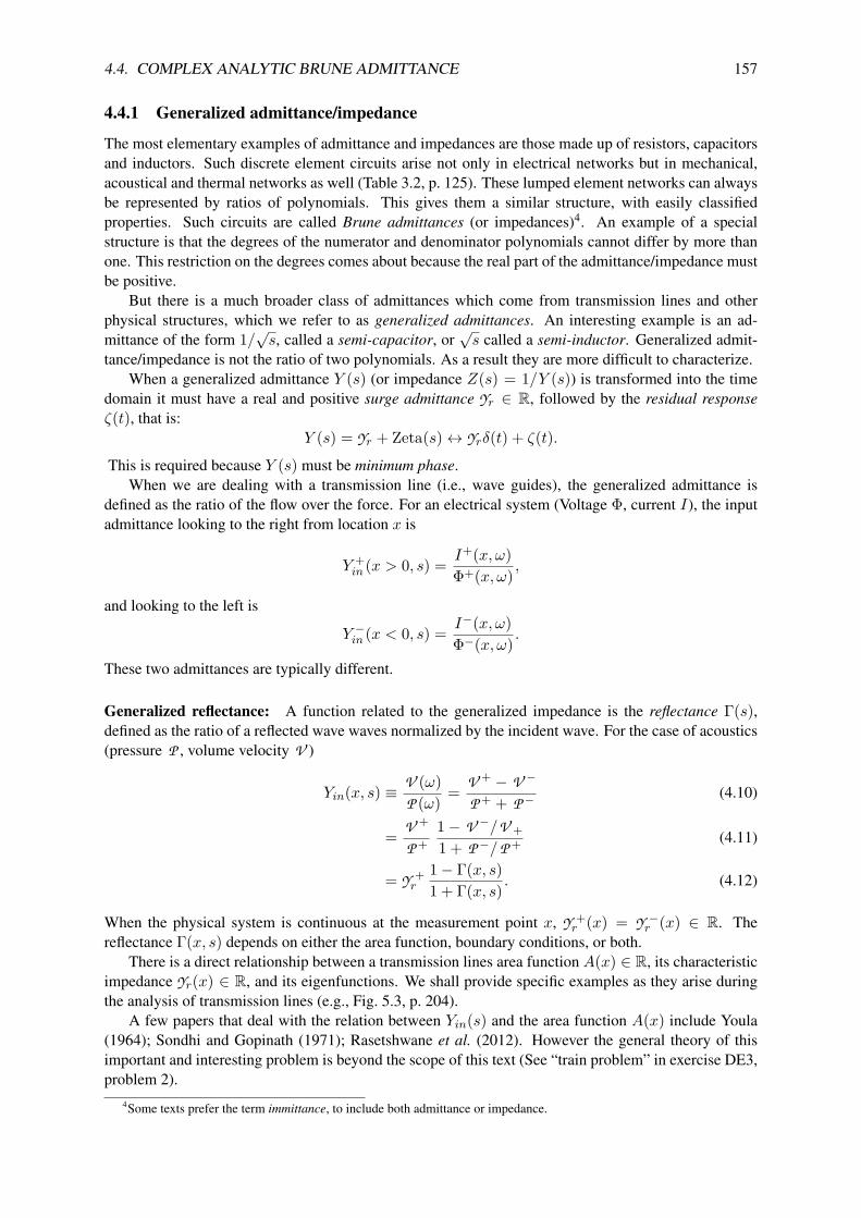
4.4. COMPLEX ANALYTIC BRUNE ADMITTANCE 157
4.4.1 Generalized admittance/impedance
The most elementary examples of admittance and impedances are those made up of resistors, capacitorsand inductors. Such discrete element circuits arise not only in electrical networks but in mechanical,acoustical and thermal networks as well (Table 3.2, p. 125). These lumped element networks can alwaysbe represented by ratios of polynomials. This gives them a similar structure, with easily classifiedproperties. Such circuits are called Brune admittances (or impedances)4. An example of a specialstructure is that the degrees of the numerator and denominator polynomials cannot differ by more thanone. This restriction on the degrees comes about because the real part of the admittance/impedance mustbe positive.
But there is a much broader class of admittances which come from transmission lines and otherphysical structures, which we refer to as generalized admittances. An interesting example is an ad-mittance of the form 1/
√s, called a semi-capacitor, or
√s called a semi-inductor. Generalized admit-
tance/impedance is not the ratio of two polynomials. As a result they are more difficult to characterize.When a generalized admittance Y (s) (or impedance Z(s) = 1/Y (s)) is transformed into the time
domain it must have a real and positive surge admittance Yr ∈ R, followed by the residual responseζ(t), that is:
Y (s) = Yr + Zeta(s)↔ Yrδ(t) + ζ(t).
This is required because Y (s) must be minimum phase.When we are dealing with a transmission line (i.e., wave guides), the generalized admittance is
defined as the ratio of the flow over the force. For an electrical system (Voltage Φ, current I), the inputadmittance looking to the right from location x is
Y +in (x > 0, s) = I+(x, ω)
Φ+(x, ω) ,
and looking to the left is
Y −in (x < 0, s) = I−(x, ω)Φ−(x, ω) .
These two admittances are typically different.
Generalized reflectance: A function related to the generalized impedance is the reflectance Γ(s),defined as the ratio of a reflected wave waves normalized by the incident wave. For the case of acoustics(pressure P , volume velocity V )
Yin(x, s) ≡ V (ω)P (ω) = V + − V −
P + + P −(4.10)
= V +
P +1− V −/V +1 + P −/P + (4.11)
= Y +r
1− Γ(x, s)1 + Γ(x, s) . (4.12)
When the physical system is continuous at the measurement point x, Y +r (x) = Y −r (x) ∈ R. The
reflectance Γ(x, s) depends on either the area function, boundary conditions, or both.There is a direct relationship between a transmission lines area function A(x) ∈ R, its characteristic
impedance Yr(x) ∈ R, and its eigenfunctions. We shall provide specific examples as they arise duringthe analysis of transmission lines (e.g., Fig. 5.3, p. 204).
A few papers that deal with the relation between Yin(s) and the area function A(x) include Youla(1964); Sondhi and Gopinath (1971); Rasetshwane et al. (2012). However the general theory of thisimportant and interesting problem is beyond the scope of this text (See “train problem” in exercise DE3,problem 2).
4Some texts prefer the term immittance, to include both admittance or impedance.

158 CHAPTER 4. STREAM 3A: SCALAR CALCULUS
Complex analytic Γ(s) and Yin(s) = Z−1in (s)
When defining the complex reflectance Γ(s) a key assumption has been made: even though Γ(s) isdefined by the ratio of two functions of real (radian) frequency ω, like the impedance, the reflectancemust be causal (postulate P1, p. 133). That γ(t) → Γ(s) and ζ(t) ↔ Zin(s) = 1/Yin(s) are causal isrequired by the physics.
4.4.2 Complex analytic impedance
Conservation of energy (or power) is a cornerstone of modern physics. It may first have been underconsideration by Galileo Galilei (1564-1642) and Marin Mersenne (1588-1648). Today the questionis not whether it is true, but why. Specifically, what is the physics behind conservation of energy?Surprisingly, the answer is straightforward, based on its definition and the properties of impedance.Recall that the power is the product of the force and flow, and impedance is their ratio.
The power is given by the product of two variables, sometimes called conjugate variables, the forceand the flow. In electrical terms, these are voltage (force) (v(t) ↔ V (ω)) and current (flow) (i(t) ↔I(ω)); thus, the electrical power at any instant of time is
P (t) = v(t)i(t). (4.13)
The total energy E(t) is the integral of the power, since P (t) = dE/dt. Thus if we start with all theelements at rest (no currents or voltages), then the energy as a function of time is always positive
E(t) =∫ t
0P (t)dt ≥ 0, (4.14)
and is simply the total energy applied to the network (Van Valkenburg, 1964a, p. 376). Since the voltageand current are related by either an impedance or an admittance, conservation of energy depends on theproperty of impedance. From Ohm’s law and P1 (every impedance is causal)
v(t) = z(t) ? i(t) =∫ t
τ=0z(τ)i(t− τ)dτ ↔ V (s) = Z(s)I(s).
Example: Let i(t) = δ(t). Then |w|2(τ) = i(t) ? i(t) = δ(τ). Thus
Ixx(t) =∫ t
τ=0z(τ)|w|2(τ)dτ =
∫ t
τ=0z(τ)δ(τ)dτ =
∫ t
0z(τ)dτ.
The Brune impedance always has the form z(t) = roδ(t) + ζ(t). The characteristic impedance (akasurge impedance) may be defined as (Lundberg et al., 2007)
ro =∫ ∞
0−z(t)dt.
This definition requires that the integral of (ζ(t)) is zero, a suspect conclusion that needs further inves-tigation.
Note that convolution by an admittance or impedance, linearizes the expression for the power.Perhaps easier to visualize is when working in the Laplace frequency domain, where the total energy,
equal to the integral of the real part of the power, is
1s<V I = 1
2s(V ∗I + V I∗) = 12s(Z∗I∗I + ZII∗) = 1
s<Z(s)|I|2 ≥ 0.
Mathematically this is called a positive definite operator, since the positive and real resistance is sand-wiched between the current, forcing the definiteness.
In conclusion, conservation of energy is totally dependent on the properties of the impedance. Thusone of the most important and obvious applications of complex functions of a complex variable is theimpedance function. This seems to be the ultimate example of the FTCC, applied to z(t).
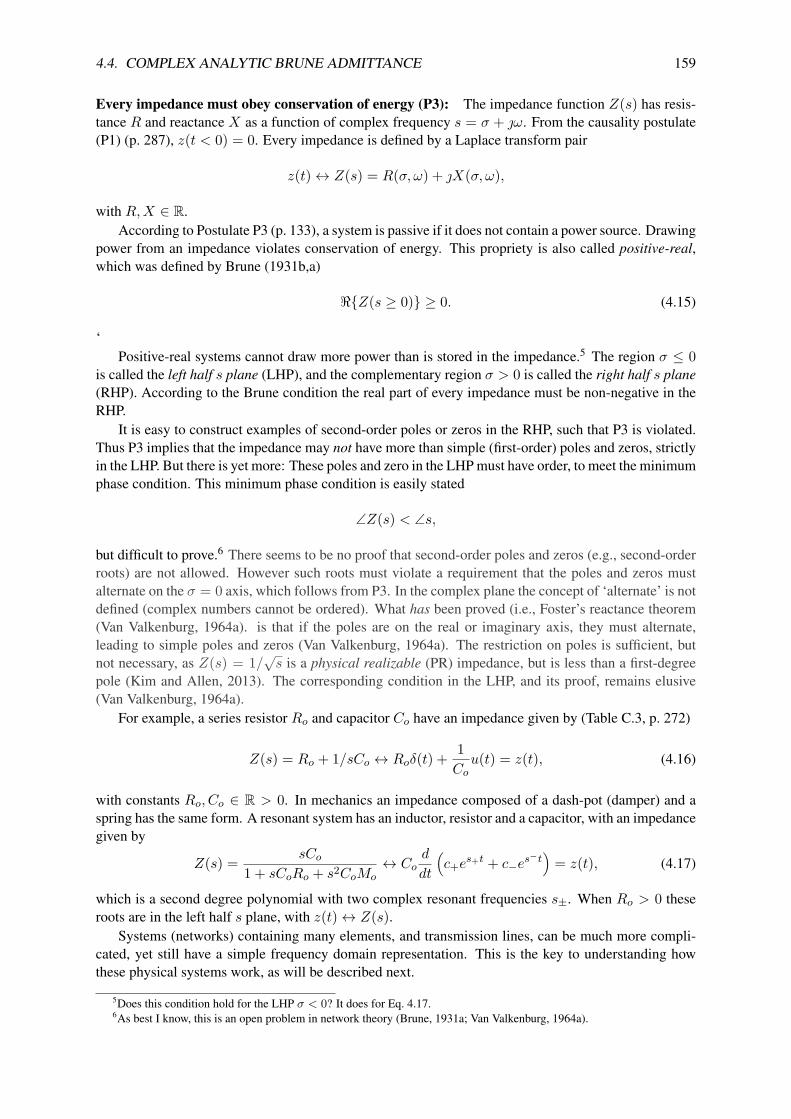
4.4. COMPLEX ANALYTIC BRUNE ADMITTANCE 159
Every impedance must obey conservation of energy (P3): The impedance function Z(s) has resis-tance R and reactance X as a function of complex frequency s = σ + ω. From the causality postulate(P1) (p. 287), z(t < 0) = 0. Every impedance is defined by a Laplace transform pair
z(t)↔ Z(s) = R(σ, ω) + X(σ, ω),
with R,X ∈ R.According to Postulate P3 (p. 133), a system is passive if it does not contain a power source. Drawing
power from an impedance violates conservation of energy. This propriety is also called positive-real,which was defined by Brune (1931b,a)
<Z(s ≥ 0) ≥ 0. (4.15)
‘Positive-real systems cannot draw more power than is stored in the impedance.5 The region σ ≤ 0
is called the left half s plane (LHP), and the complementary region σ > 0 is called the right half s plane(RHP). According to the Brune condition the real part of every impedance must be non-negative in theRHP.
It is easy to construct examples of second-order poles or zeros in the RHP, such that P3 is violated.Thus P3 implies that the impedance may not have more than simple (first-order) poles and zeros, strictlyin the LHP. But there is yet more: These poles and zero in the LHP must have order, to meet the minimumphase condition. This minimum phase condition is easily stated
∠Z(s) < ∠s,
but difficult to prove.6 There seems to be no proof that second-order poles and zeros (e.g., second-orderroots) are not allowed. However such roots must violate a requirement that the poles and zeros mustalternate on the σ = 0 axis, which follows from P3. In the complex plane the concept of ‘alternate’ is notdefined (complex numbers cannot be ordered). What has been proved (i.e., Foster’s reactance theorem(Van Valkenburg, 1964a). is that if the poles are on the real or imaginary axis, they must alternate,leading to simple poles and zeros (Van Valkenburg, 1964a). The restriction on poles is sufficient, butnot necessary, as Z(s) = 1/
√s is a physical realizable (PR) impedance, but is less than a first-degree
pole (Kim and Allen, 2013). The corresponding condition in the LHP, and its proof, remains elusive(Van Valkenburg, 1964a).
For example, a series resistor Ro and capacitor Co have an impedance given by (Table C.3, p. 272)
Z(s) = Ro + 1/sCo ↔ Roδ(t) + 1Cou(t) = z(t), (4.16)
with constants Ro, Co ∈ R > 0. In mechanics an impedance composed of a dash-pot (damper) and aspring has the same form. A resonant system has an inductor, resistor and a capacitor, with an impedancegiven by
Z(s) = sCo1 + sCoRo + s2CoMo
↔ Cod
dt
(c+e
s+t + c−es−t)
= z(t), (4.17)
which is a second degree polynomial with two complex resonant frequencies s±. When Ro > 0 theseroots are in the left half s plane, with z(t)↔ Z(s).
Systems (networks) containing many elements, and transmission lines, can be much more compli-cated, yet still have a simple frequency domain representation. This is the key to understanding howthese physical systems work, as will be described next.
5Does this condition hold for the LHP σ < 0? It does for Eq. 4.17.6As best I know, this is an open problem in network theory (Brune, 1931a; Van Valkenburg, 1964a).

160 CHAPTER 4. STREAM 3A: SCALAR CALCULUS
Poles and zeros of positive real functions must be first degree: The definition of positive real (PR)functions requires that the poles and the zeros of the impedance function be simple (only first degree).Second degree poles would have a reactive “secular” response of the form h(t) = t sin(ωkt + φ)u(t),and these terms would not average to zero, depending on the phase, as is required of an impedance. Asa result, only single degree poles are possible.7 Furthermore, when the impedance is the ratio of twopolynomials, where the lower degree polynomial is the derivative of the higher degree one, then thepoles and zeros must alternate. This is a well-known property of the Brune impedance that has neverbeen adequately explained except for very special cases, denoted as Foster’s theorem (Van Valkenburg,1964b, p. 104-107). I believe that no one has ever reported an impedance having second degree polesand zeros. That would be a rare impedance. Network analysis books never report 2nd degree poles andzeros in their impedance functions. Nor has there ever been any guidance as to where the poles andzeros might lie in the left-hand s plane. Understanding the exact relationships between pairs of polesand zeros, to assure that the real part of the impedance is real, would resolve this longstanding unsolvedproblem (Van Valkenburg, 1964b).
Complex analytic functions: To solve a differential equation, or integrate a function, Newton usedthe Taylor series to integrate one term at a time. However, he only used real functions of a real variable,due to the fundamental lack of appreciation of the complex analytic function. This same method is howone finds solutions to scalar differential equations today, but using an approach that makes the solutionmethod less obvious. Rather than working directly with the Taylor series, today we use the complexexponential, since the complex exponential is an eigen-function of the derivative
d
dtest = sest.
Since est may be expressed as a Taylor series, having coefficients cn = 1/n!, in some real sense themodern approach is a compact way of doing what Newton did. Thus every linear constant coefficientdifferential equation in time may be simply transformed into a polynomial in complex Laplace frequencys, by looking for solutions of the form A(s)est, transforming the differential equation into a polynomialA(s) in complex frequency. For example,
d
dtf(t) + af(t)↔ (s+ a)F (s).
The root of A(sr) = sr + a = 0 is the eigenvalue of the differential equation. A powerful tool forunderstanding the solutions of differential equations, both scalar and vector, is to work in the Laplacefrequency domain. The Taylor series has been replaced by est, transforming Newton’s real Taylor seriesinto the complex exponential eigen-function. In some sense, these are the same method, since
est =∞∑n=0
(st)n
n! . (4.18)
Taking the derivative with respect to time gives
d
dtest = sest = s
∞∑n=0
(st)n
n! , (4.19)
which is also complex analytic. Thus if the series for F (s) is valid (i.e., it converges), then its derivativeis also valid. This was a very powerful concept, exploited by Newton for real functions of a real variable,and later by Cauchy and Riemann for complex functions of a complex variable. The key question hereis: Where does the series fail to converge? This is the main message behind the FTCC (Eq. 4.8).
The FTCC (Eq. 4.5) is formally the same as the FTC (Eq. 4.7) (Leibniz formula), the key (andsignificant) difference being that the argument of the integrand s ∈ C. Thus this integration is a line
7Secular terms result from second degree poles since u(t) ? u(t) = tu(t)↔ 1/s2.

4.4. COMPLEX ANALYTIC BRUNE ADMITTANCE 161
integral in the complex plane. One would naturally assume that the value of the integral depends on thepath of integration. And it does, but in a subtle way, as quantified by Cauchy’s various theorems. Ifthe path says in the same RoC region, then the integral is independent of that path. If a path includes adifferent pole, then the integral depends on the path, as quantified by the Cauchy residue theorem. Thetest is to deform the path from the first to the second. If in that deformation the path crosses a pole,thenthe integral will depend on the path. All of this is dependent of the causal nature of the integral.
But, according to the FTCC, it does not. In fact they are clearly distinguishable from the FTC. Andthe reasoning is the same. If F (s) = df(s)/ds is complex analytic (i.e., has a power series f(s) =∑k cks
k, with f(s), ck, s ∈ C), then it may be integrated, and yet integral does not depend on the path.At first blush, this is sort of amazing. The key is that F (s) and f(s) must be complex analytic, whichmeans they are differentiable. This all follows from the Taylor series formula Eq. 4.10 (p. 148) for thecoefficients of the complex analytic series. For Eq. 4.8 to hold, the derivatives must be independent ofthe direction (independent of the path), as discussed on page 149. The concept of a complex analyticfunction therefore has eminent consequences, in the form of several key theorems on complex integrationdiscovered by Cauchy (c1820).
The use of the complex Taylor series generalizes the functions it describes, with unpredictable con-sequences, as nicely shown by the domain coloring diagrams presented on p. 135. Cauchy’s tools ofcomplex integration were first exploited in physics by Sommerfeld (1952) to explain the onset (e.g.,causal) transients in waves, as explained in detail in Brillouin (1960, Chap. 3).
Up to 1910, when Sommerfeld first published his results using complex analytic signals and saddlepoint integration in the complex plane, there was a poor understanding of the implications of the causalwave-front. It would be reasonable to say that his insights changed our understanding of wave propaga-tion, for both light and sound. Sadly this insight has never been fully appreciated, even to this day. Ifyou question this review, please read Brillouin (1960, Chap. 1).
Figure 4.2: Here we show the mapping for the square root func-tion z = ±
√x, the inverse of x = z2. This function has two
single-valued sheets of the x plane corresponding to the two signs ofthe square root. The best way to view this function is in polar co-ordinates, with x = |x|eφ and z =
√|x|eφ/2. Figure from:
https://en.wikipedia.org/wiki/Riemann surface
The full power of the complex an-alytic function was first appreciatedby Bernard Riemann (1826-1866) inhis University of Gottingen PhD the-sis of 1851, under the tutelage of CarlFriedrich Gauss (1777-1855), whichdrew heavily on the work of Cauchy.
The key definition of a complex an-alytic function is that it has a Taylor se-ries representation over a region of thecomplex frequency plane s = σ + jω,that converges in a region of conver-gence (RoC) about the expansion point,with a radius determined by the near-est pole of the function. A further sur-prising feature of all analytic functionsis that within the RoC, the inverse ofthat function also has a complex ana-lytic expansion. Thus given w(s), one may also determine s(w) to any desired accuracy, criticallydepending on the RoC. Given the right software (e.g., zviz.m), this relationship may be made precise.
4.4.3 Multi-valued functions
In the field of mathematics there seems to have been a tug-of-war regarding the basic definition ofthe concept of a function. The accepted definition today seems to be a single-valued (i.e., complex

162 CHAPTER 4. STREAM 3A: SCALAR CALCULUS
analytic) mapping from the domain to the codomain (or range). This makes the discussion of multi-valued functions somewhat awkward. In 1851 Riemann (working with Gauss) seems to have resolvedthis problem for the complex analytic set of multi-valued functions by introducing the concept of single-valued sheets, delineated by branch-cuts.
Two simple yet important examples of multi-valued functions are the circle z2 = x2 + y2 andw = log(z). For example, assuming z is the radius of the circle, solving for y(x) gives the double-valued function
y(x) = ±√z2 − x2.
The related function z = ±√x is shown in Fig. 4.2 as a three-dimensional display, in polar coordinates,
with y(r) as the vertical axis, as a function of the angle and radius of x ∈ C.If we accept the modern definition of a function as the mapping from one set to a second, then
y(x) is not a function, or even two functions. For example, what if x > z? Or worse, what if z = 2with |x| < 1? Riemann’s construction, using branch cuts for multivalued function, resolves all thesedifficulties (as best I know).
To proceed, we need definitions and classifications of the various types of complex singularities:
1. Poles of degree 1 are called simple poles. Their amplitude is called the residue (e.g. α/s hasresidue α). Simple poles are special (Eq. 4.24, p. 167), as they play a key role in mathematicalphysics, since their inverse Laplace transform defines a causal eigen-function.
2. When the numerator and denominator of a rational function (i.e., ratio of two polynomials) havea common root (i.e., factor), that root is said to be removable.
3. A singularity that is not (1) removable, (2) a pole or (3) a branch point is called essential.
4. A complex analytic function (except for isolated poles), is called meromorphic Boas (1987).Meromorphic functions can have any number of poles, even an infinite number. The poles neednot be simple.
5. When the first derivative of a function Z(s) has a simple pole at a, then a is said to be a branchpoint of Z(s). An important example is the logarithmic derivative
d ln(s− a)α/ds = α/(s− a), α ∈ I.
However, the converse does not necessarily hold.
6. I am not clear about the interesting case of an irrational pole (α ∈ I). In some cases (e.g., α ∈ F)this may be simplified via the logarithmic derivative operation, as mentioned above.
More complex topologies are being researched today, and progress is expected to accelerate due tomodern computing technology.8 It is helpful to identify the physical meaning of these more complexsurfaces, to guide us in their interpretation and possible applications.9
Branch cuts: Up to this point we have only considered poles of degree α ∈ N of the form 1/sα.The concept of a branch cut allows one to manipulate (and visualize) multi-valued functions, for whichα ∈ F. This is done by breaking each region into single-valued sheets, as shown in Fig. 4.3 (right). Thebranch cut is a curve ∈ C that separates the various single-valued sheets of a multi-valued function. Theconcepts of branch cuts, sheets and the extended plane were first devised by Riemann, working withGauss (1777-1855), as first described in his thesis of 1851. It was these three mathematical and geomet-rical constructions that provided the deep insight into complex analytic functions, greatly extending theimportant earlier work of Cauchy (1789-1857) on the calculus of complex analytic functions. For alter-native helpful discussion of Riemann sheets and branch cuts, see Boas (1987, Section 29, pp. 221-225)and (Kusse and Westwig, 2010).
8https://www.maths.ox.ac.uk/about-us/departmental-art/theory9https://www.quantamagazine.org/secret-link-uncovered-between-pure-math-and-physics-20171201
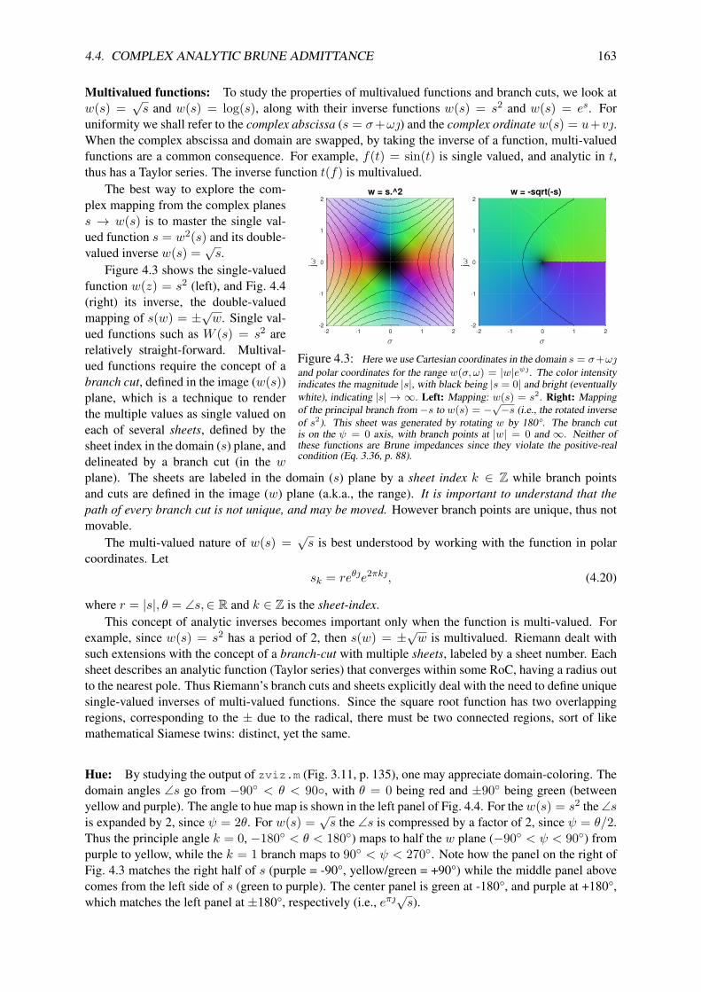
4.4. COMPLEX ANALYTIC BRUNE ADMITTANCE 163
Multivalued functions: To study the properties of multivalued functions and branch cuts, we look atw(s) =
√s and w(s) = log(s), along with their inverse functions w(s) = s2 and w(s) = es. For
uniformity we shall refer to the complex abscissa (s = σ+ω) and the complex ordinate w(s) = u+v.When the complex abscissa and domain are swapped, by taking the inverse of a function, multi-valuedfunctions are a common consequence. For example, f(t) = sin(t) is single valued, and analytic in t,thus has a Taylor series. The inverse function t(f) is multivalued.
w = s.^2
σ
-2 -1 0 1 2
jω
2
1
0
-1
-2
w = -sqrt(-s)
σ
-2 -1 0 1 2
jω
2
1
0
-1
-2
Figure 4.3: Here we use Cartesian coordinates in the domain s = σ+ωand polar coordinates for the range w(σ, ω) = |w|eψ. The color intensityindicates the magnitude |s|, with black being |s = 0| and bright (eventuallywhite), indicating |s| → ∞. Left: Mapping: w(s) = s2. Right: Mappingof the principal branch from −s to w(s) = −
√−s (i.e., the rotated inverse
of s2). This sheet was generated by rotating w by 180°. The branch cutis on the ψ = 0 axis, with branch points at |w| = 0 and ∞. Neither ofthese functions are Brune impedances since they violate the positive-realcondition (Eq. 3.36, p. 88).
The best way to explore the com-plex mapping from the complex planess → w(s) is to master the single val-ued function s = w2(s) and its double-valued inverse w(s) =
√s.
Figure 4.3 shows the single-valuedfunction w(z) = s2 (left), and Fig. 4.4(right) its inverse, the double-valuedmapping of s(w) = ±
√w. Single val-
ued functions such as W (s) = s2 arerelatively straight-forward. Multival-ued functions require the concept of abranch cut, defined in the image (w(s))plane, which is a technique to renderthe multiple values as single valued oneach of several sheets, defined by thesheet index in the domain (s) plane, anddelineated by a branch cut (in the wplane). The sheets are labeled in the domain (s) plane by a sheet index k ∈ Z while branch pointsand cuts are defined in the image (w) plane (a.k.a., the range). It is important to understand that thepath of every branch cut is not unique, and may be moved. However branch points are unique, thus notmovable.
The multi-valued nature of w(s) =√s is best understood by working with the function in polar
coordinates. Letsk = reθe2πk, (4.20)
where r = |s|, θ = ∠s,∈ R and k ∈ Z is the sheet-index.This concept of analytic inverses becomes important only when the function is multi-valued. For
example, since w(s) = s2 has a period of 2, then s(w) = ±√w is multivalued. Riemann dealt with
such extensions with the concept of a branch-cut with multiple sheets, labeled by a sheet number. Eachsheet describes an analytic function (Taylor series) that converges within some RoC, having a radius outto the nearest pole. Thus Riemann’s branch cuts and sheets explicitly deal with the need to define uniquesingle-valued inverses of multi-valued functions. Since the square root function has two overlappingregions, corresponding to the ± due to the radical, there must be two connected regions, sort of likemathematical Siamese twins: distinct, yet the same.
Hue: By studying the output of zviz.m (Fig. 3.11, p. 135), one may appreciate domain-coloring. Thedomain angles ∠s go from −90 < θ < 90, with θ = 0 being red and ±90 being green (betweenyellow and purple). The angle to hue map is shown in the left panel of Fig. 4.4. For thew(s) = s2 the ∠sis expanded by 2, since ψ = 2θ. For w(s) =
√s the ∠s is compressed by a factor of 2, since ψ = θ/2.
Thus the principle angle k = 0, −180 < θ < 180) maps to half the w plane (−90 < ψ < 90) frompurple to yellow, while the k = 1 branch maps to 90 < ψ < 270. Note how the panel on the right ofFig. 4.3 matches the right half of s (purple = -90°, yellow/green = +90°) while the middle panel abovecomes from the left side of s (green to purple). The center panel is green at -180°, and purple at +180°,which matches the left panel at ±180°, respectively (i.e., eπ
√s).
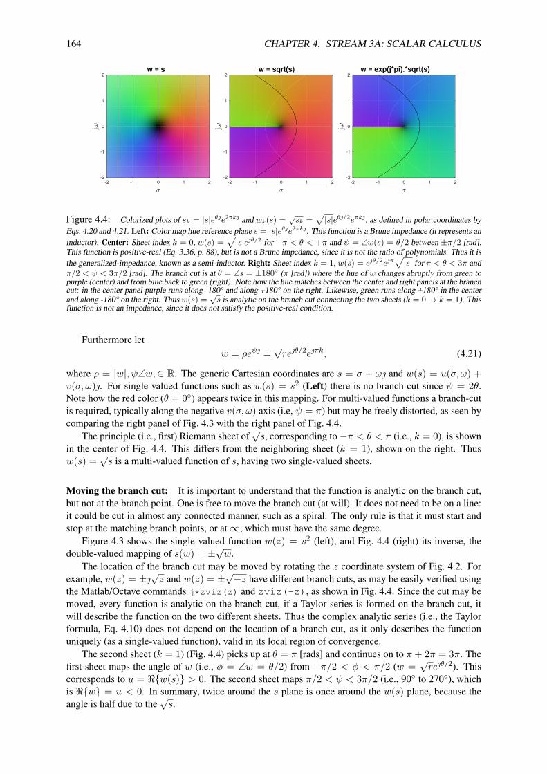
164 CHAPTER 4. STREAM 3A: SCALAR CALCULUS
w = s
σ
-2 -1 0 1 2
jω
2
1
0
-1
-2
w = sqrt(s)
σ
-2 -1 0 1 2
jω
2
1
0
-1
-2
w = exp(j*pi).*sqrt(s)
σ
-2 -1 0 1 2
jω
2
1
0
-1
-2
Figure 4.4: Colorized plots of sk = |s|eθe2πk and wk(s) = √sk =√|s|eθ/2eπk, as defined in polar coordinates by
Eqs. 4.20 and 4.21. Left: Color map hue reference plane s = |s|eθe2πk. This function is a Brune impedance (it represents aninductor). Center: Sheet index k = 0, w(s) =
√|s|eθ/2 for −π < θ < +π and ψ = ∠w(s) = θ/2 between ±π/2 [rad].
This function is positive-real (Eq. 3.36, p. 88), but is not a Brune impedance, since it is not the ratio of polynomials. Thus it isthe generalized-impedance, known as a semi-inductor. Right: Sheet index k = 1, w(s) = eθ/2eπ
√|s| for π < θ < 3π and
π/2 < ψ < 3π/2 [rad]. The branch cut is at θ = ∠s = ±180 (π [rad]) where the hue of w changes abruptly from green topurple (center) and from blue back to green (right). Note how the hue matches between the center and right panels at the branchcut: in the center panel purple runs along -180° and along +180° on the right. Likewise, green runs along +180° in the centerand along -180° on the right. Thus w(s) =
√s is analytic on the branch cut connecting the two sheets (k = 0→ k = 1). This
function is not an impedance, since it does not satisfy the positive-real condition.
Furthermore letw = ρeψ =
√reθ/2eπk, (4.21)
where ρ = |w|, ψ∠w,∈ R. The generic Cartesian coordinates are s = σ + ω and w(s) = u(σ, ω) +v(σ, ω). For single valued functions such as w(s) = s2 (Left) there is no branch cut since ψ = 2θ.Note how the red color (θ = 0) appears twice in this mapping. For multi-valued functions a branch-cutis required, typically along the negative v(σ, ω) axis (i.e, ψ = π) but may be freely distorted, as seen bycomparing the right panel of Fig. 4.3 with the right panel of Fig. 4.4.
The principle (i.e., first) Riemann sheet of√s, corresponding to −π < θ < π (i.e., k = 0), is shown
in the center of Fig. 4.4. This differs from the neighboring sheet (k = 1), shown on the right. Thusw(s) =
√s is a multi-valued function of s, having two single-valued sheets.
Moving the branch cut: It is important to understand that the function is analytic on the branch cut,but not at the branch point. One is free to move the branch cut (at will). It does not need to be on a line:it could be cut in almost any connected manner, such as a spiral. The only rule is that it must start andstop at the matching branch points, or at∞, which must have the same degree.
Figure 4.3 shows the single-valued function w(z) = s2 (left), and Fig. 4.4 (right) its inverse, thedouble-valued mapping of s(w) = ±
√w.
The location of the branch cut may be moved by rotating the z coordinate system of Fig. 4.2. Forexample, w(z) = ±
√z and w(z) = ±
√−z have different branch cuts, as may be easily verified using
the Matlab/Octave commands j*zviz(z) and zviz(-z), as shown in Fig. 4.4. Since the cut may bemoved, every function is analytic on the branch cut, if a Taylor series is formed on the branch cut, itwill describe the function on the two different sheets. Thus the complex analytic series (i.e., the Taylorformula, Eq. 4.10) does not depend on the location of a branch cut, as it only describes the functionuniquely (as a single-valued function), valid in its local region of convergence.
The second sheet (k = 1) (Fig. 4.4) picks up at θ = π [rads] and continues on to π + 2π = 3π. Thefirst sheet maps the angle of w (i.e., φ = ∠w = θ/2) from −π/2 < φ < π/2 (w =
√reθ/2). This
corresponds to u = <w(s) > 0. The second sheet maps π/2 < ψ < 3π/2 (i.e., 90 to 270), whichis <w = u < 0. In summary, twice around the s plane is once around the w(s) plane, because theangle is half due to the
√s.

4.4. COMPLEX ANALYTIC BRUNE ADMITTANCE 165
Branch cuts emanate and terminate at branch points, defined as singularities (poles), that can evenhave fractional degree, as for example 1/
√s, and terminate at one of the matching roots, which includes
the possibility of∞.10 For example, suppose that in the neighborhood of the pole, at so the function is
f(s) = w(s)(s− so)k
,
wherew, s, so ∈ C and k ∈ Q. When k = 1, so = σo+ωo is a first degree “simple pole”, having degree1 in the s plane, with residue w(so).11 Typically the order and degree are positive integers, but fractionaldegrees and orders are common in modern engineering applications (Kirchhoff, 1868; Lighthill, 1978).Here we shall allow both the degree and order to be fractional (∈ F). When k ∈ F ⊂ R (k = n/m isa real reduced fraction. Namely when GCD(n,m)=1, n ⊥ m). This defines the degree of a fractionalpole. In such cases there must be two sets of branch cuts of degree n and m. For example, if k = 1/2,the singularity (branch cut) is of degree 1/2, and there are two Riemann sheets, as shown in Fig. 4.3
w = sqrt(pi./s)
σ
-2 -1 0 1 2
jω
2
1
0
-1
-2
w = sqrt(s.^2+1)
σ
-2 -1 0 1 2
jω
2
1
0
-1
-2
Figure 4.5: Colorized plots of two LT pairs: Left:√π/s↔ u(t)/
√t. Right:
√s2 + 1↔ δ(t) + 1
tJ1(t)u(t).
Fractional-order Bessel function: An important example is the Bessel function
δ(t) + 1tJ1(t)u(t)↔
√s2 + 1,
as shown in Fig. 4.5, which is related to the solution to the wave equation in two-dimensional cylindricalcoordinates (Table C.4, p. 273). Bessel functions are the solutions (i.e., eigen-functions) of guidedacoustic waves in round pipes, or surface waves on the earth (seismic waves), or waves on the surface ofa pond (Table 5.2, p. 214).
There are a limited number of possibilities for the degree, k ∈ Z or ∈ F. If the degree is drawnfrom R 6∈ F, the pole cannot not have a residue. According to the definition of the residue, k ∈ F willnot give a residue. But there remains open the possibility of generalizing the concept of the Riemannintegral theorem, to include k ∈ F. One way to do this is to use the logarithmic derivative which rendersfractional poles to simple poles with fractional residues.
If the singularity has an irrational degree (k ∈ I), the branch cut has the same “irrational degree.”Accordingly there would be an infinite number of Riemann sheets, as in the case of the log function. Anexample is k = π, for which
F (s) = 1sπ
= e− log(sπ) = e−π log(s) = e−π log(ρ)e−πθ,
10This presumes that poles appear in pairs, one of which may be at∞.11We shall refer to the order of a derivative, or differential equation, and the degree of a polynomial, as commonly used in
engineering applications.

166 CHAPTER 4. STREAM 3A: SCALAR CALCULUS
where the domain is expressed in polar coordinates s = ρeθ. When k ∈ F it may be close (e.g.,k = π152/π153 = π152/(π152 + 2) = 881/883 ≈ 0.99883, or its reciprocal ≈ 1.0023). The branch cutcould be very subtle (it could even go unnoticed), but it would have a significant impact on the function,and on its inverse Laplace transform.
Example: Find poles, zeros and residues of F (s).
1.
F (s) = d
dsln s+ e
s+ π,
Solution:F (s) = d
ds[ln(s+ e)− ln(s+ π)] =
( 1s+ e
− 1s+ π
)The the poles are at s1 = −e and s2 = −π with respective residues of ±1.
2.
F (s) = d
dsln (s+ 3)e
(s+ )−π ,
Solution:F (s) = d
ds(e ln(s+ 3) + π ln(s+ )) = e
s+ 3 + π
s+ .
There is a very important take-home message here regarding the utility of thelogarithmic derivative, which “linearizes” the fractional pole.
3.F (s) = eπ ln s,
Solution: Taking the derivative
d
dsF (s) = d
dsln sπ = π
d
dsln s = π
s.
Thus we see that F ′(s) has a pole at s = 0 with residue π. It follows that F (s) =∫ s F ′(s)ds has
a second order pole. Thus the residue must be zero.
4.F (s) = π−s.
Solution: Taking the logarithmic derivative, d lnF (s)/ds = F ′(s)/F (s) = − ln π.
Thus F ′(s) = − ln πF (s) = − ln π π−s. )
Log function: Next we discuss the multi-valued nature of the log function. In this case there are aninfinite number of Riemann sheets, not well captured by Fig. 3.13 (p. 137), which displays only theprincipal sheet. However, if we look at the formula for the log function, the nature is easily discerned.The abscissa s may be defined as multi-valued since
sk = re2πkeθ.
Here we have extended the angle of s by 2πk, where k is the sheet index ∈ Z. Taking the log
log(s) = log(r) + (θ + 2πk).
When k = 0 we have the principal value sheet, which is zero when s = 1. For any other value of k,w(s) 6= 0, even when r = 1, since the angle is not zero, except for the k = 0 sheet.

4.5. THREE COMPLEX INTEGRATION THEOREMS I 167
4.5 Three Cauchy integral theorems
4.5.1 Cauchy’s theorems for integration in the complex plane
There are three basic definitions related to Cauchy’s integral formula. They are closely related, and cangreatly simplify integration in the complex plane. The choice of names seems unfortunate, if not totallyconfusing.
1. Cauchy’s (integral) theorem (CT-1): ∮CF (s)ds = 0, (4.22)
if and only if F (s) is complex analytic inside of a simple closed curve C (Boas, 1987, p. 45);(Stillwell, 2010, 319). The FTCC (Eq. 4.8) says that the integral only depends on the end pointsif F (s) is complex analytic. By closing the path (contour C ) the end points are the same, thus theintegral must be zero, as long as F (s) is complex analytic.
2. Cauchy’s integral formula (CT-2):
12πj
∮B
F (s)s− so
ds =F (so), so ∈ C < B (inside)0, so 6∈ C > B (outside).
(4.23)
Here F (s) is required to be analytic everywhere within (and on) the boundary B of integration(Greenberg, 1988, p. 1200); (Boas, 1987, p. 51); (Stillwell, 2010, p. 220). When the point so ∈ Cis within the boundary the value F (so) ∈ C is the residue of the pole so of F (s)/(s− so). Whenthe point so lies outside the boundary, the integral is zero.
3. The (Cauchy) residue theorem (CT-3): (Greenberg, 1988, p. 1241), (Boas, 1987, p. 73)
∮CF (s)ds = 2πj
K∑k=1
ck =K∑k=1
∮F (s)s− sk
ds, (4.24)
where the residues ck ∈ C corresponds to the kth pole of f(s) enclosed by the contour C . By theuse of Cauchy’s integral formula, the right-most form of the residue theorem is equivalent to theCIF.12
How to calculate the residue: The case of first degree poles has special significance, because theBrune impedance only allows simple poles and zeros, increasing its utility. The residues for simple polesare F (sk), which is complex analytic in the neighborhood of the pole, but not at the pole.
Consider the function f(s) = F (s)/(s− sk), where we have factored f(s) to isolate the first-orderpole at s = sk, with F (s) analytic at sk. Then the residue of the poles at ck = F (sk). This coefficientis computed by removing the singularity, by placing a zero at the pole frequency, and taking the limit ass→ sk, namely
ck = lims→sk
[(s− sk)F (s)] (4.25)
(Greenberg, 1988, p. 1242), (Boas, 1987, p. 72).When the pole is anN th degree, the procedure is much more complicated, and requires takingN−1
order derivatives of f(s), followed by the limit process (Greenberg, 1988, p. 1242). Higher degree polesare rarely encountered; thus, it is good to know that this formula exists, but perhaps it is not worth theeffort to learn (i.e., memorize) it.
12This theorem is the same as a 2D version of Stokes’s theorem (Boas, 1987).

168 CHAPTER 4. STREAM 3A: SCALAR CALCULUS
Summary and examples: These three theorems, all attributed to Cauchy, collectively are related tothe fundamental theorems of calculus. Because the names of the three theorems are so similar, they areeasily confused.
1. In general it makes no sense (nor is there any need) to integrate through a pole, thus the poles (orother singularities) must not lie on C .
2. Theorem CT-1 (Eq. 4.22) follows trivially from the fundamental theorem of complex calculus(Eq. 4.8, p. 148), since if the integral is independent of the path, and the path returns to the startingpoint, the closed integral must be zero. Thus Eq. 4.22 holds when F (s) is complex analytic withinC.
3. Since the real and imaginary parts of every complex analytic function obey Laplace’s equation(Eq. 4.15, p. 150), it follows that every closed integral over a Laplace field, i.e., one defined byLaplace’s equation, must be zero. In fact this is the property of a conservative system, corre-sponding to many physical systems. If a closed box has fixed potentials on the walls, with anydistribution whatsoever, and a point charge (i.e., an electron) is placed in the box, then a forceequal to F = qE is required to move that charge, and thus work is done. However, if the point isreturned to its starting location, the net work done is zero.
4. Work is done in charging a capacitor, and energy is stored. However, when the capacitor isdischarged, all of the energy is returned to the load.
5. Soap bubbles and rubber sheets on a wire frame obey Laplace’s equation.
6. These are all cases where the fields are Laplacian, thus closed line integrals must be zero. Lapla-cian fields are commonly observed because they are so basic.
7. We have presented the impedance as the primary example of a complex analytic function. Phys-ically, every impedance has an associated stored energy, and every system having stored energyhas an associated impedance. This impedance is usually defined in the frequency s domain, as aforce over a flow (i.e., voltage over current). The power P (t) is defined as the force times the flowand the energy E (t) as the time integral of the power
E (t) =∫ t
−∞P (t)dt, (4.26)
which is similar to Eq. 4.6 (p. 147) [see Section 3.7.3, Eq. 3.15 (p. 124)]. In summary, impedanceand power and energy are all fundamentally related.
4.6. EXERCISES DE-2 169
4.6 Exercises DE-2
Topic of this homework:
Integration of complex functions; Cauchy’s theorem, integral formula, residue theorem; power series;Riemann sheets and branch cuts; inverse Laplace transforms
Problem # 1: FTCC and integration in the complex planeRecall that, according to the Fundamental Theorem of Complex Calculus (FTCC),
f(z) = f(z0) +∫ z
z0F (ζ)dζ, (4.1)
where z0, z, ζ, F ∈ C. It follows that
F (z) = d
dzf(z). (4.2)
Thus Eq. 4.3 is also known as the anti-derivative of f(z).
–Q 1.1: For a closed interval a, b, the FTCC can be stated as∫ b
aF (z)dz = f(b)− f(a), (4.3)
meaning that the result of the integral is independent of the path from x = a to x = b. What condition(s)on the integrand f(z) is (are) sufficient to assure that Eq. 4.3 holds?
–Q 1.2: For the function f(z) = cz, where c ∈ C is an arbitrary complex constant, use theCauchy-Riemann (CR) equations to show that f(z) is analytic for all z ∈ C.
Problem # 2: In the following problems, solve the integral
I =∫
CF (z)dz
for a given path C . In some cases this might be the definite integral (Eq. 4.3).Let the function F (z) = cz , where c ∈ C is given for each problem below. Hint: Can you apply the
FTCC?
–Q 2.1: Find the anti-derivative of F (z).
–Q 2.2: c = 1/e = 1/2.7183 . . . where C is ζ = 0→ i→ z
–Q 2.3: c = 2 where C is ζ = 0→ (1 + i)→ z
–Q 2.4: c = i where the path C is an inward spiral described by z(t) = 0.99tei2πt fort = 0→ t0 →∞

170 CHAPTER 4. STREAM 3A: SCALAR CALCULUS
–Q 2.5: c = et−τ0 where τ0 > 0 is a real number, and C is z = (1 − i∞) → (1 + i∞).Hint: Do you recognize this integral? If you do not recognize the integral, please do not spenda lot of time trying to solve it via the ‘brute force’ method.
Problem # 3: Cauchy’s theorems for integration in the complex planeThere are three basic definitions related to Cauchy’s integral formula. They are all related, and cangreatly simplify integration in the complex plane. When a function depends on a complex variable weshall use uppercase notation, consistent with the engineering literature for the Laplace transform.
1. Cauchy’s (Integral) Theorem (Stillwell, p. 319; Boas, p. 45)∮CF (z)dz = 0,
if and only if F (z) is complex-analytic inside of C .
This is related to the Fundamental Theorem of Complex Calculus (FTCC)
f(z) = f(a) +∫ z
aF (z)dz,
where f(z) is the anti-derivative of F (z), namely F (z) = df/dz. The FTCC requires F (z)to be complex-analytic for all z ∈ C. By closing the path (contour C ), Cauchy’s theorem (andthe following theorems) allows us to integrate functions that may not be complex-analytic for allz ∈ C.
2. Cauchy’s Integral Formula (Boas, p. 51; Stillwell, p. 220)
12πj
∮C
F (z)z − z0
dz =F (z0), z0 ∈ C (inside)0, z0 6∈ C (outside)
Here F (z) is required to be analytic everywhere within (and on) the contour C . F (z0) is calledthe residue of the pole.
3. (Cauchy’s) Residue Theorem (Boas, p. 72)
∮CF (z)dz = 2πj
K∑k=1
Resk,
where Resk are the residues of all poles of F (z) enclosed by the contour C .
How to calculate the residues: The residues can be rigorously defined as
Resk = limz→zk
[(z − zk)f(z)].
This can be related to Cauchy’s integral formula: Consider the function F (z) = w(z)/(z − zk),where we have factored F (z) to isolate the first-order pole at z = zk. If the remaining factor w(z)is analytic at zk, then the residue of the pole at z = zk is w(zk).
–Q 3.1: Describe the relationships between the three theorems:
1. (1) and (2)
2. (1) and (3)

4.6. EXERCISES DE-2 171
3. (2) and (3)
–Q 3.2: Consider the function with poles at z = ±j
F (z) = 11 + z2 = 1
(z − j)(z + j)Find the residue expansion.
–Q 3.3: Apply Cauchy’s theorems to solve the following integrals.State which theorem(s) you used, and show your work.
1.∮
C F (z)dz where C is a circle centered at z = 0 with a radius of 12 .
2.∮
C F (z)dz where C is a circle centered at z = j with a radius of 1.
3.∮
C F (z)dz where C is a circle centered at z = 0 with a radius of 2.
Problem # 4: Integration in the complex planeIn the following questions, you’ll be asked to integrate F (s) = u(σ, ω) + iv(σ, ω) around the contour Cfor complex s = σ + iω, ∮
CF (s)ds.
Follow the directions carefully for each question. When asked to state where the function is and is notanalytic, you are not required to use the Cauchy-Riemann equations (but you should if you can’t answerthe question ‘by inspection’).
–Q 4.1: F (s) = sin(s)
–Q 4.2: Given function F (s) = 1s
1. State where the function is and is not analytic.
2. Explicitly evaluate the integral when C is the unit circle, defined as s = eiθ, 0 ≤ θ ≤ 2π.
3. Evaluate the same integral using Cauchy’s theorem and/or the residue theorem.
–Q 4.3: F (s) = 1s2
1. State where the function is and is not analytic.
2. Explicitly evaluate the integral when C is the unit circle, defined as s = eiθ, 0 ≤ θ ≤ 2π.
3. What does your result imply about the residue of the 2nd order pole at s = 0?
–Q 4.4: F (s) = est
1. State where the function is and is not analytic.
2. Explicitly evaluate the integral when C is the square (σ, ω) = (1, 1) → (−1, 1) → (−1,−1) →(1,−1)→ (1, 1).
3. Evaluate the same integral using Cauchy’s theorem and/or the residue theorem.

172 CHAPTER 4. STREAM 3A: SCALAR CALCULUS
–Q 4.5: F (s) = 1s+2
1. State where the function is and is not analytic.
2. Let C be the unit circle, defined as s = eiθ, 0 ≤ θ ≤ 2π. Evaluate the integral using Cauchy’stheorem and/or the residue theorem.
3. Let C be a circle of radius 3, defined as s = 3eiθ, 0 ≤ θ ≤ 2π. Evaluate the integral usingCauchy’s theorem and/or the residue theorem.
–Q 4.6: F (s) = 12πi
est
(s+4)
1. State where the function is and is not analytic.
2. Let C be a circle of radius 3, defined as s = 3eiθ, 0 ≤ θ ≤ 2π. Evaluate the integral usingCauchy’s theorem and/or the residue theorem.
3. Let C contain the entire left-half s-plane. Evaluate the integral using Cauchy’s theorem and/or theresidue theorem. Do you recognize this integral?
–Q 4.7: F (s) = ± 1√s
(e.g. F 2 = 1s)
1. State where the function is and is not analytic.
2. This function is multivalued. How many Riemann sheets do you need in the domain (s) and therange (f ) to fully represent this function? Indicate (e.g. using a sketch) how the sheet(s) in thedomain map to the sheet(s) in the range.
3. Explicitly evaluate the integral ∫C
1√zdz
when C is the unit circle, defined as s = eiθ, 0 ≤ θ ≤ 2π. Is this contour ‘closed’? State why orwhy not.
4. Explicitly evaluate the integral ∫C
1√zdz
when C is twice around the unit circle, defined as s = eiθ, 0 ≤ θ ≤ 4π. Is this contour ‘closed’?State why or why not. Hint: Note that√
ei(θ+2π) =√ei2πeiθ = eiπ
√eiθ = −1
√eiθ
5. What does your result imply about the residue of the (twice-around 12 order) pole at s = 0?
6. Show that the residue is zero. Hint: apply the definition of the residue.
Problem # 5: A two-port network application for the Laplace transform
Recall that the Laplace transform (LT ) f(t)↔ F (s)13 of a causal function f(t) is
F (s) =∫ ∞
0−f(t)e−stdt,
13Many loosely adhere to the convention that the frequency domain uses upper-case [e.g. F (s)] while the time domain useslower case [f(t)]

4.6. EXERCISES DE-2 173
where s = σ + jω is complex frequency14 in [radians] and t is time in [seconds]. Causal functionsand the Laplace transform are particularly useful for describing systems, which have no response until asignal enters the system (e.g. at t = 0).
The definition of the inverse Laplace transform (LT −1) requires integration in the complex plane:
f(t) = 12πj
∫ σ0+j∞
σ0−j∞F (s)estds = 1
2πj
∮CF (s)estds.
The Laplace contour C actually includes two pieces∮C
=∫ σ0+j∞
σ0−j∞+∫⊂∞
,
where the path represented by ‘⊂∞’ is a semicircle of infinite radius with σ → −∞. It is somewhattricky to do, but it may be proved that the integral over the contour ⊂∞ goes to zero. For a causal,‘stable’ (e.g. doesn’t blow up over time) signal, all of the poles of F (s) must be inside of the Laplacecontour, in the left-half s-plane.
Transfer functions Linear, time-invariant systems are described by an ordinary differential equations.For example, consider the first-order linear differential equation
a1d
dty(t) = b1
d
dtx(t) + b0x(t). (4.4)
This equation describes the relationship between the input (x(t)) and output (y(t)) of the system. If wedefine Laplace transforms y(t) ↔ Y (s) and x(t) ↔ X(s), then this equation may be written in thefrequency domain as
a1sY (s) = b1sX(s) + b0X(s).
The transfer function for this system is defined as
H(s) = Y (s)X(s) = b1s+ b0
a1s= b1a1
+ b0a1s
.
In this problem, we will look at the transfer function of a simple two-port network, shown in Figure 4.6.This network is an example of a RC low-pass filter, which acts as a leaky integrator.
+
−
+
−
R1 R2
I1
V1 V2
C I2
Figure 4.6: This three-element electrical circuit is a system that acts to low-pass filter the signal voltage V1(ω), to producesignal V2(ω).
Problem # 6: ABCD method
14While radians are useful units for calculations, when providing physical insight in discussions of problem solutions, it iseasier to work with Hertz, since frequency in [Hz] and time in [s] are mentally more more natural units than radians. The sameis true of degrees vs. radians. Boas (p. 10) recommends the use degrees over radians. He gives the example of 3π/5 [radians],which is more easily visualize as 108.
174 CHAPTER 4. STREAM 3A: SCALAR CALCULUS
–Q 6.1: Low-pass RC filter
1. Use the ABCD method to find the matrix representation of Fig. 4.6.
2. Assuming that I2 = 0, find the transfer function H(s) ≡ V2/V1. From the results of the ABCDmatrix you determined above, show that
H(s) = 11 +R1Cs
.
3. The transfer function H(s) has one pole. Where is the pole? Find the residue of this pole.
4. Find h(t), the inverse Laplace transform of H(s).
5. Assuming that V2 = 0 find Y12(s) ≡ I2/V1.
6. Find the input impedance to the right-hand side of the system, Z22(s) ≡ V2/I2 for two cases:
(a) I1 = 0(b) V1 = 0
7. Compute the determinant of the ABCD matrix. Hint: It is always 1.
8. Compute the derivative of H(s) = V2V1
∣∣∣I2=0
.
Problem # 7:With the help of a computerIn the following problems, we will look at some of the concepts from this homework using Matlab/Oc-tave. We are using the syms function which requires Matlab’s/Octave’s symbolic math toolbox. Or youmay use the EWS lab’s Matlab. Alternative symbolic-math tool, such as Wolfram Alpha.15
Example: To find the Taylor series expansion about s = 0 of
F (s) = − log(1− s),
first consider the derivative and its Taylor series (about s = 0)
F ′(s) = 11− s =
∞∑n=0
sn.
Then, integrate this series term by term
F (s) = − log(1− s) =∫ s
F ′(s)ds =∞∑n=0
sn
n.
Alternatively you may use Matlab/Octave commands:
syms staylor(-log(1-s),’order’,7)
–Q 7.1: Use Octave’s taylor(-log(1-s)) to 7th order, as in the example above.
1. Try the above Matlab/Octave commands. Give the first 7 terms of the Taylor series (confirm thatMatlab/Octave agrees with the formula derived above).
15https://www.wolframalpha.com/

4.6. EXERCISES DE-2 175
2. What is the inverse Laplace transform of this series? Consider the series term by term.
–Q 7.2: The function 1/√z has a branch point at z = 0, thus it is singular there.
1. Can you apply Cauchy’s integral theorem when integrating around the unit circle?
2. Below is a Matlab/Octave code that computes∫ 4π
0dz√z
using Matlab’s/Octave’s symbolic analysispackage:
syms zI=int(1/sqrt(z))J = int(1/sqrt(z),exp(-j*pi),exp(j*pi))eval(J)
Run this script. What answers do you get for I and J?
3. Modify this code to integrate f(z) = 1/z2 once around the unit circle. What answers do you getfor I and J?
–Q 7.3: Bessel functions can describe waves in a cylindrical geometryThe Bessel function has a Laplace transform with a branch cut
J0(t)u(t)↔ 1√1 + s2
.
Draw a hand sketch showing the nature of the branch cut. Hint: Use zviz.
Problem # 8: Matlab/Octave exercises:
–Q 8.1: Comment on the following Matlab/Octave exercises
1. Try the following Matlab/Octave commands, and then comment on your findings.
%Take the inverse LT of 1/sqrt(1+sˆ2)syms sI=ilaplace(1/(sqrt((1+sˆ2))));disp(I)
%Find the Taylor series of the LTT = taylor(1/sqrt(1+sˆ2),10); disp(T);
%Verify thissyms tJ=laplace(besselj(0,t));disp(J);
%plot the Bessel functiont=0:0.1:10*pi;b=besselj(0,t);plot(t/pi,b);grid on;
–Q 8.2: When did Friedrich Bessel live?
–Q 8.3: What did he use Bessel functions for?
–Q 8.4: Using zviz, for each of the following functions
1. Describe the plot generated by zviz S=Z.

176 CHAPTER 4. STREAM 3A: SCALAR CALCULUS
2. Are the functions defined below legal Brune impedances? (i.e., Do they function obey <Z(σ >0) ≥ 0)? Hint: Consider the phase (color). Plot zviz Z for a reminder of the colormap.
1. zviz 1./sqrt(1+S.ˆ2)
2. zviz 1./sqrt(1-S.ˆ2)
3. zviz 1./(1+sqrt(S)))
Problem # 9: Find the LT −1 of one factor of the Riemann zeta function ζp(s)where ζp(s)↔ zp(t) and describe your results in words.
Hint: Consider the geometric series representation
ζp(s) = 11− e−sTp =
∞∑k=0
e−skTp , (4.5)
for which you can look up the LT −1 transform of each term.
Problem # 10: Inverse transform of products:The time domain version of Eq. 4.5 (p. 176) may be written as the convolution of all the zk(t) factors
z(t) ≡ z2(t) ? z3(t) ? z5(t) ? z7(t) · · · ? zp(t) ? · · · , (4.6)
where ? represents time convolution.
++
Tp
i(t) = q(t)− (1/α)q(t− Tp)q(t) = αq(n− Tp) + v(t)
q(t− Tp)
q(t)v(t) i(t)
α −1/α
Figure 4.7: This feedback network is described by a time-domain difference equation with delay Tp, has an all-pole transferfunction ζp(s) ≡ Q(s)/I(s) given by Eq. 4.7, which physically corresponds to a stub of a transmission line, with the inputat one end and the output at the other. To describe the ζ(s) function we must take α = −1. A transfer function Y (s) =V (s)/I(s) that has the same poles as ζp(s), but with zeros as given by Eq. 4.8, is the input admittance Y (s) = I(s)/V (s) ofthe transmission line, defined at the ratio of the Laplace transform of the current i(t)↔ I(s) over the voltage v(t)↔ V (s).
Explain what this means in physical terms. Start with two terms (e.g., z1(t) ? z2).
Physical interpretation: Such functions may be generated in the time domain as shown in Fig. 4.7(p. 176), using a feedback delay of Tp seconds described by the two equations in the figure with a unityfeedback gain α = −1. Taking the Laplace transform of the system equation we see that the transferfunction between the state variable q(t) and the input x(t) is given by ζp(s), which is and all-polefunction, since
Q(s) = e−sTnQ(s) + V (s), or ζp(s) ≡Q(s)V (s) = 1
1− e−sTp . (4.7)
Closing the feed-forward path gives a second transfer function Y (s) = I(s)/V (s), namely
Y (s) ≡ I(s)V (s) = 1− e−sTp
1 + e−sTp. (4.8)

4.6. EXERCISES DE-2 177
If we take i(t) as the current and v(t) as the voltage at the input to the transmission line, then yp(t) ↔ζp(s) represents the input impedance at the input to the line. The poles and zeros of the impedanceinterleave along the jω axis. By a slight modification ζp(s) may alternatively be written as
Yp(s) = esTp/2 + e−sTp/2
esTp/2 − e−sTp/2= j tan(sTp/2). (4.9)
Every impedance Z(s) has a corresponding reflectance function given by a Mobius transformation,which may be read off of Eq. 4.8 as
Γ(s) ≡ 1 + Z(s)1− Z(s) = e−sTp (4.10)
since impedance is also related to the round-trip delay Tp on the line. The inverse Laplace transform ofΓ(s) is the round trip delay Tp on the line
γ(t) = δ(t− Tp)↔ e−sTp . (4.11)
Working in the time domain provides a key insight, as it allows us to parse out the best analyticcontinuation of the infinity of possible continuations, that are not obvious in the frequency domain.Transforming to the time domain is a form of analytic continuation of ζ(s), that depends on the assump-tion that z(t) is one-sided in time (causal).

178 CHAPTER 4. STREAM 3A: SCALAR CALCULUS
4.6.1 Cauchy Integral Formula & Residue Theorem
CT-2 (Eq. 4.23) is an important extension of CT-1 (Eq. 4.22) in that a pole has been explicitly injectedinto the integrand at s = so. If the pole location is outside of the curve C , the result of the integral iszero, in keeping with CT-1. When the pole is inside of C , the integrand is no longer complex analyticat the enclosed pole. When this pole is simple, the residue theorem applies. By a manipulation of thecontour in CT-2, the pole can be isolated with a circle around the pole, and then taking the limit, theradius may be taken to zero, in the limit, isolating the pole.
For the related CT-3 (Eq. 4.24) the same result holds, except it is assumed that there are K simplepoles in the function F (s). This requires the repeated application of CT-2, K times, so it represents aminor extension of CT-2. The function F (s) may be written as f(s)/PK(s), where f(s) is analytic inC and PK(s) is a polynomial of degree K, with all of its roots sk ∈ C .
Non-integral degree singularities: The key point is that this theorem applies when n ∈ I, includingfractionals n ∈ F; but for these cases the residue is always zero, since by definition, the residue is theamplitude of the 1/s term (Boas, 1987, p. 73).
Examples:
1. When n ∈ F (e.g., n = 2/3), the residue of sn is zero, by definition.
2. The function 1/√s has a zero residue (apply the definition of the residue Eq. 4.25).
3. When n 6= 1 ∈ I, the residue is, by definition, zero.
4. When n = 1, the residue is given by Eq. 4.25.
5. CT-1, 2, 3 are essential when computing the inverse Laplace transform.
4.7 Inverse Laplace transform (t < 0): Cauchy’s residue theorem
The inverse Laplace transform Eq. 3.24 transforms a function of complex frequency F (s) and returns acausal function of time f(t)
f(t)↔ F (s),
where f(t) = 0 for t < 0. Examples are provided in Table C.3 (p. 272). We next discuss the detailsof finding the inverse transform by use of CT-3, and how the causal requirement f(t < 0) = 0 comesabout.
The integrand of the inverse transform is F (s)est and the limits of integration are −σo∓ω. To findthe inverse we must close the curve, at infinity, and specify that the integral at ω → ∞. There are twoways to close these limits – to the right σ > 0 (RHP), and to the left σ < 0 (LHP) – but there needsto be some logical reason for this choice. That logic is determined by the sign of t. For the integral toconverge, the term est must go to zero as ω →∞. In terms of the real and imaginary parts of s = σ+ω,the exponential may be rewritten as eσteωt. Note that both t and ω go to ∞. So it is the interactionbetween these two limits that determines how we pick the closure, RHP vs. LHP.
Case for causality (t < 0): Let us first consider negative time, including t → −∞. If we were toclose C in the left half-plane (σ < 0), then the product σt is positive (σ < 0, t < 0, thus σt > 0). Inthis case as ω → ∞, the closure integral |s| → ∞ will diverge. Thus we may not close in the LHP fornegative time. If we close in the RHP σ > 0 then the product σt < 0 and est will go to zero as ω →∞.This then justifies closing the contour, allowing for the use of the Cauchy theorems.
If F (s) is analytic in the RHP, the FTCC applies, and the resulting f(t) must be zero, and the inverseLaplace transform must be causal. This argument holds for any F (s) that is analytic in the RHP (σ > 0).

4.7. INVERSE LAPLACE TRANSFORM 179
Case of unstable poles: An important but subtle point arises: If F (s) has a pole in the RHP, then theabove argument still applies if we pick σo to be to the right of the RHP pole. This means that the inversetransform may still be applied to unstable poles (those in the RHP). This explains the need for the σo inthe limits. If F (s) has no RHP poles, then σo = 0 is adequate, and this factor may be ignored.
Case for zero time (t = 0): When time is zero, the integral does not, in general, converge, leavingf(t) undefined. This is most clear in the case of the step function u(t) ↔ 1/s, where the integral maynot be closed, because the convergence factor est = 1 is lost for t = 0.
The fact that u(t) does not exist at t = 0 explains the Gibbs phenomenon in the inverse Fouriertransform. At times where a jump occurs, the derivative of the function does not exist, and thus the timeresponse function is not analytic. The Fourier expansion cannot converge at places where the functionis not analytic. A low-pass filter may be used to smooth the function, but at the cost of temporal reso-lution. Forcing the function to be analytic at the discontinuity, by smoothing the jumps, is an importantcomputational method.
4.7.1 Inverse Laplace transform (t > 0)
Case of t > 0: Next we investigate the convergence of the integral for positive time t > 0. In this casewe must close the integral in the LHP (σ < 0) for convergence, so that st < 0 (σ ≤ 0 and t > 0). Whenthere are poles on the ω = 0 axis, σo > 0 assures convergence by keeping the on-axis poles inside thecontour. At this point CT-3 is relevant. If we restrict ourselves to simple poles (as required for a Bruneimpedance), the residue theorem may be directly applied.
The most simple example is the step function, for which F (s) = 1/s and thus
u(t) =∮
LHP
est
s
ds
2π ↔1s,
which is a direct application of the CI-3, Eq. 4.24 (p. 167). The forward transform of u(t) is straightfor-ward, as discussed on p. 131. This is true of most if not all of the elementary forward Laplace transforms.In these cases, causality is built into the integral by its limits. An interesting problem is how to provethat u(t) is not defined at t = 0.
s = cos(pi*z)
x-2 -1 0 1 2
jy
2
1
0
-1
-2
s = besselj(0,pi*z)
x-2 -1 0 1 2
jy
2
1
0
-1
-2
Figure 4.8: Left: Colorized plot of w(z) = sin(z). Right: Colorized plot of w(z) = Jo(πz). Note the similarity of thetwo functions. The first Bessel zero is at 2.405, and thus appears at 0.7655 = 2.405/π, about 1.53 times larger than the rootof cos(πz) at 1/2. Other than this minor distortion of the first few roots, the two functions are basically identical. It followsthat their LT ’s must have similar characteristics, as documented in Table C.4 (p. 273).
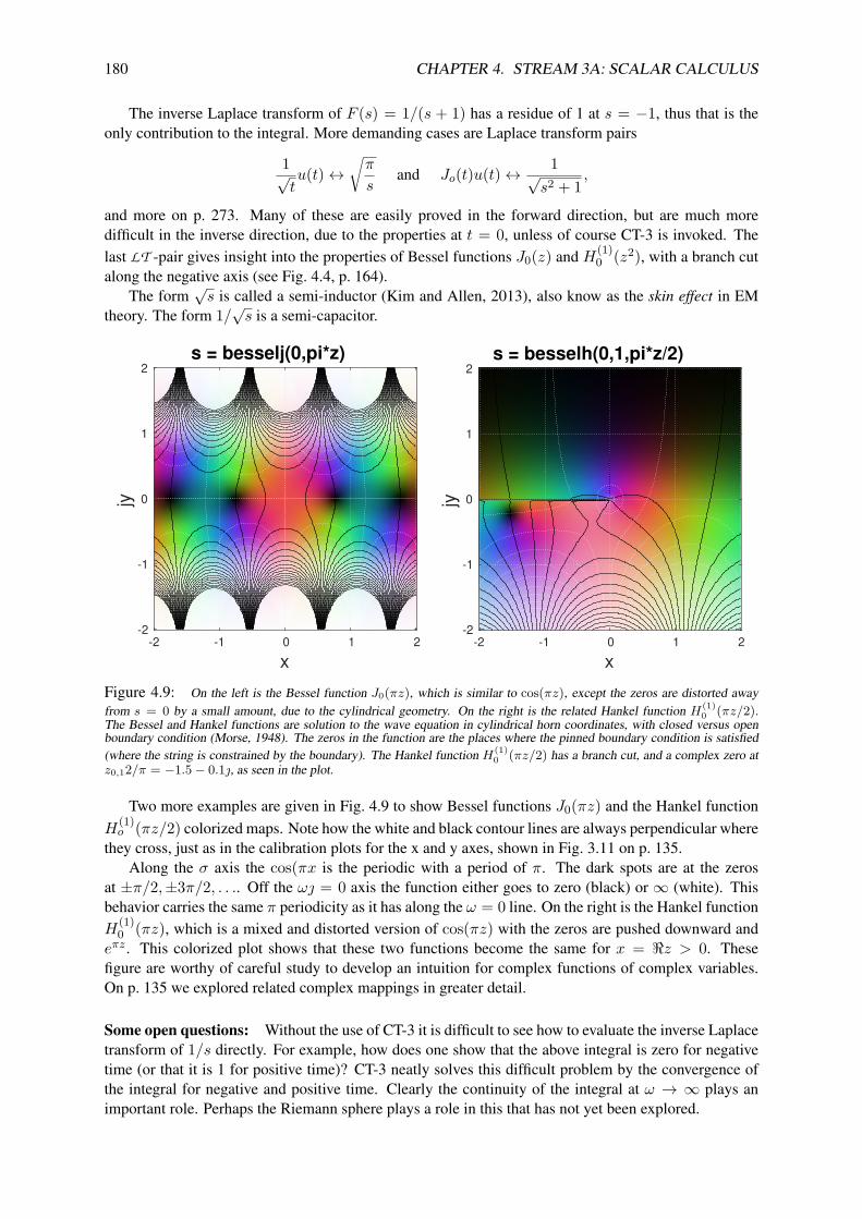
180 CHAPTER 4. STREAM 3A: SCALAR CALCULUS
The inverse Laplace transform of F (s) = 1/(s + 1) has a residue of 1 at s = −1, thus that is theonly contribution to the integral. More demanding cases are Laplace transform pairs
1√tu(t)↔
√π
sand Jo(t)u(t)↔ 1√
s2 + 1,
and more on p. 273. Many of these are easily proved in the forward direction, but are much moredifficult in the inverse direction, due to the properties at t = 0, unless of course CT-3 is invoked. Thelast LT -pair gives insight into the properties of Bessel functions J0(z) and H(1)
0 (z2), with a branch cutalong the negative axis (see Fig. 4.4, p. 164).
The form√s is called a semi-inductor (Kim and Allen, 2013), also know as the skin effect in EM
theory. The form 1/√s is a semi-capacitor.
s = besselj(0,pi*z)
x-2 -1 0 1 2
jy
2
1
0
-1
-2
s = besselh(0,1,pi*z/2)
x-2 -1 0 1 2
jy
2
1
0
-1
-2
Figure 4.9: On the left is the Bessel function J0(πz), which is similar to cos(πz), except the zeros are distorted awayfrom s = 0 by a small amount, due to the cylindrical geometry. On the right is the related Hankel function H(1)
0 (πz/2).The Bessel and Hankel functions are solution to the wave equation in cylindrical horn coordinates, with closed versus openboundary condition (Morse, 1948). The zeros in the function are the places where the pinned boundary condition is satisfied(where the string is constrained by the boundary). The Hankel function H(1)
0 (πz/2) has a branch cut, and a complex zero atz0,12/π = −1.5− 0.1, as seen in the plot.
Two more examples are given in Fig. 4.9 to show Bessel functions J0(πz) and the Hankel functionH
(1)o (πz/2) colorized maps. Note how the white and black contour lines are always perpendicular where
they cross, just as in the calibration plots for the x and y axes, shown in Fig. 3.11 on p. 135.Along the σ axis the cos(πx is the periodic with a period of π. The dark spots are at the zeros
at ±π/2,±3π/2, . . .. Off the ω = 0 axis the function either goes to zero (black) or∞ (white). Thisbehavior carries the same π periodicity as it has along the ω = 0 line. On the right is the Hankel functionH
(1)0 (πz), which is a mixed and distorted version of cos(πz) with the zeros are pushed downward and
eπz . This colorized plot shows that these two functions become the same for x = <z > 0. Thesefigure are worthy of careful study to develop an intuition for complex functions of complex variables.On p. 135 we explored related complex mappings in greater detail.
Some open questions: Without the use of CT-3 it is difficult to see how to evaluate the inverse Laplacetransform of 1/s directly. For example, how does one show that the above integral is zero for negativetime (or that it is 1 for positive time)? CT-3 neatly solves this difficult problem by the convergence ofthe integral for negative and positive time. Clearly the continuity of the integral at ω → ∞ plays animportant role. Perhaps the Riemann sphere plays a role in this that has not yet been explored.

4.7. INVERSE LAPLACE TRANSFORM 181
4.7.2 Properties of the LT (e.g., Linearity, convolution, time-shift, modulation, etc.)
As shown in the table of Laplace transforms, there are integral (i.e., integration, not integer) relation-ships, or properties, that are helpful to identify. The first of these is a definition, not a property:
f(t)↔ F (s).
When taking the LT, the time response is given in lower case (e.g., f(t)) and the frequency domaintransform is denoted in upper case (e.g., F (s)). It is required, but not always explicitly specified, thatf(t < 0) = 0, that is, the time function must be causal.
Linearity: The most basic property is the linearity (superposition) property of the LT , summarizedby P2.
Convolution property: The product of two LT s in frequency results in convolution in time
f(t) ? g(t) =∫ t
0f(τ)g(t− τ)dτ ↔ F (s)G(s),
where we use the ? operator as a shorthand for the convolution of two time functions.A key application of convolution is filtering, which takes many forms. The most basic filter is the
moving average, the moving sum of data samples, normalized by the number of samples. Such a filterhas very poor performance. It also introduces a delay of half the length of the average, which may ormay not constitute a problem, depending on the application. Another important example is a low-passfilter that removes high-frequency noise, or a notch filter that removes line-noise (i.e., 60 [Hz] in the US,and its 2nd and 3d harmonics, 120 and 180 [Hz]). Such noise is typically a result of poor grounding andground loops. It is better to solve the problem at its root than to remove it with a notch filter. Still, filtersare very important in engineering.
By taking the LT of the convolution we can derive this relationship:
∫ ∞0
[f(t) ? g(t)]e−stdt =∫ ∞t=0
[∫ t
0f(τ)g(t− τ)dτ
]e−stdt
=∫ t
0f(τ)
(∫ ∞t=0
g(t− τ)e−stdt)dτ
=∫ t
0f(τ)
(e−sτ
∫ ∞t′=0
g(t′)e−st′dt′)dτ
= G(s)∫ t
0f(τ)e−sτdτ
= G(s)F (s).
We first encountered this relationship on p. 99 in the context of multiplying polynomials, which wasthe same as convolving their coefficients. The parallel should be obvious. In the case of polynomials,the convolution was discrete in the coefficients, and here it is continuous in time. But the relationshipsare the same.
Time-shift property: When a function is time-shifted by time To, the LT is modified by esTo , leadingto the property
f(t− To)↔ e−sTo F (s).
This is easily shown by applying the definition of the LT to a delayed time function.

182 CHAPTER 4. STREAM 3A: SCALAR CALCULUS
Time derivative: The key to the eigen-function analysis provided by the LT is the transformation of atime derivative on a time function, that is,
d
dtf(t)↔ sF (s).
Here s is the eigenvalue corresponding to the time derivative of est. Given the definition of the derivativeof est with respect to time, this definition seems trivial. Yet that definition was not obvious to Euler. Itneeded to be extended to the space of complex analytic function est, which did not happen until at leastRiemann (1851).
Given a differential equation of order K, the LT results in a polynomial in s, of degree K. It followsthat this LT property is the corner-stone of why the LT is so important to scalar differential equations, asit was to the early analysis of Pell’s equation and the Fibonacci sequence, as presented in earlier chapters.This property was first uncovered by Euler. It is not clear if he fully appreciated its significance, but bythe time of his death, it certainly would have been clear to him. Who first coined the terms eigenvalueand eigen-function? The word eigen is a German word meaning of one.
Initial and final value theorems: There are much more subtle relations between f(t) and F (s) thatcharacterize f(0+) and f(t→∞). While these properties can be very important in certain applications,they are beyond the scope of the present treatment. These relate to so-called initial value theorems. Ifthe system under investigation has potential energy at t = 0, then the voltage (velocity) need not be zerofor negative time. An example is a charged capacitor or a moving mass. These are important situations,but better explored in a more in-depth treatment.
4.7.3 Solving differential equations: Method of Forbenius
Many differential equations may be solved by assuming a power series (i.e., Taylor series) solution ofthe form
y(x) = xr∞∑n=0
cnxn (4.12)
with r ∈ Z and coefficients cn ∈ C. The method of Forbenius is quite general (Greenberg, 1988, p. 193).
Example: When a solution of this form is substituted into the differential equation, a recursion relationin the coefficients results. For example, if the equation is
y′′(x) = λ2y(x)
the recursion is cn = cn−1/n. The resulting equation is
y(x) = eλx = x0∞∑n=0
1n!x
n,
namely cn = 1/n!, thus ncn = 1/(n− 1)! = cn−1.
Exercise: Find the recursion relation for y(x) = Jν(x) of order ν, that satisfies Bessel’s equation
x2y′′(x) + xy′(x) + (x2 − ν2)y(x) = 0.
Solution: If we assume a complex analytic solution of the form Eq. 4.12, we find the Bessel recursionrelation for coefficients ck to be (Greenberg, 1988, p. 231).
ck = − 1k(k + 2ν)ck−2.

4.8. EXERCISES DE-3 183
4.8 Exercises DE-3
Brune Impedance
Problem # 1: Residue formA Brune impedance is defined as the ratio of the force F (s) over the flow V (s), and may be expressedin residue form as
Z(s) = c0 +K∑k=1
cks− sk
= N(s)D(s) (4.1)
with
D(s) =K∏k=1
(s− sk) and ck = lims→sk
(s− sk)D(s) =K−1∏n′=1
(s− sn).
The prime on index n′ means that n = k is not included in the product.
–Q 1.1: Find the Laplace transform (LT ) of a 1) spring, 2) dashpot and 3) mass.Express these in terms of the force F (s) and the velocity V(s), along with the electrical equivalentimpedance:
1. Hooke’s Law f(t) = Kx(t).
2. Dash-pot resistance f(t) = Rv(t).
3. Newton’s Law for Mass f(t) = Mdv(t)/dt.
–Q 1.2: Take the Laplace transform (LT ) of Eq. 3.25 (p. 132), and find the total impedanceZ(s) of the mechanical circuit.
–Q 1.3: What are N(s) and D(s) (e.g. Eq. 4.1)?
–Q 1.4: Assume thatM = R = K = 1, find the residue form of the admittance Y (s) = 1/Z(s)(e.g. Eq. 4.1) in terms of the roots s±.You may check your answer with the Matlab’s residue command.
–Q 1.5: By applying the CRT, find the inverse Laplace transform (LT −1). Use the residueform of the expression that you derived in the previous exercise.
Problem # 2: Train-mission-line We wish to model the dynamics of a freight-train having Nsuch cars, and study the velocity transfer function under various load conditions.As shown in Fig. 4.10, the train model consists of masses connected by springs.

184 CHAPTER 4. STREAM 3A: SCALAR CALCULUS
M M
K K K
MM
f1 f2 f3 f4
φ1 φ2 φ3 φ412M
12M
C
Figure 4.10: Depiction of a train consisting of cars, treated as a mass M and linkages, treated as springs of stiffness K orcompliance C = 1/K. Below it is the electrical equivalent circuit, for comparison. The mass is modeled as an inductor andthe springs as capacitors to ground. The velocity is analogous to a current and the force fn(t) to the voltage φn(t). The lengthof each cell is ∆ [m]. The train may be accurately modeled as a transmission line (TL), since the equivalent electrical circuit isa lumped model of a TL. This method, called a Cauer synthesis, is based on the ABCD transmission line method of Secs. 3.7(p. 121).
Physical description:
Use the ABCD method (see discussion in Appendix B.3, p. 265) to find the matrix representation of thesystem of Fig. 4.10. Define the force on the nth train car fn(t)↔ Fn(ω), and velocity vn(t)↔ Vn(ω).
Break the model into cells consisting of three elements: a series inductor representing half the mass(M/2), a shunt capacitor representing the spring (C = 1/K), and another series inductor representinghalf the mass (L = M/2). Making the model a cascade of symmetric A = D identical cell matrix T (s).
–Q 2.1: Find the elements of the ABCD matrix T for the single cell that relate the inputnode 1 to output node 2(Force, Velocity): [
F1V1
]= T
[F2(ω)−V2(ω)
]. (4.2)
–Q 2.2: Express each element of T (s) in terms of the the complex “Nyquist” ratio s/sc < 1(s = 2πjf , sc = 2πjfc). The Nyquist sampling cutoff frequency fc is defined in terms theminimum number of cells (i.e., 2) of length ∆ per wavelength:The Nyquest sampling theorm says that there are at least two cars per wavelength (more than two timesamples at the highest frequency). From the figure, the distance between cars ∆ = coTo [m] where
co = 1√MC
. [m/s]
The cutoff frequency obeys fcλc = co where the Nyquist wavelength is λc = 2∆. Therefore the Nyquistsampling condition is
ω < 2πfc ≡2πcoλc
= 2πco2∆ = π
∆√MC
. [Hz] (4.3)
–Q 2.3: Use the property of the Nyquist sampling frequency (Eq. 4.3) to remove higherorder powers of frequency
1 +
0(s
sc
)2≈ 1 (4.4)
to determine a band-limited approximation of T (s).
Problem # 3Now consider the cascade of N such T (s) matrices, and perform an eigen analysis.
–Q 3.1: Find the eigenvalues and eigenvectors of T (s), as functions of s/sc. Note that theformulae for the eigenvalues, eigenvectors and eigenmatrix are given above the problem setup.

4.8. EXERCISES DE-3 185
Problem # 4Finally, find the velocity transfer function:
–Q 4.1: Assuming that N = 2 and that F2 = 0 (two half-mass problem), find the transferfunction H(s) ≡ V2/V1. From the results of the T matrix you determined above, find
H21(s) = V2V1
∣∣∣∣F2=0
Express H12 in terms of a residue expansion.
–Q 4.2: Find h21(t)↔ H21(s).
–Q 4.3: What is the input impedance Z2 = F2/V2 assuming F3 = −r0V3?
–Q 4.4: Simplify the expression for Z2 assuming:
1. N →∞
2. The characteristic impedance r0 =√M/C
3. F3 = −r0V3 (i.e., −V3 cancels),
4. Ignore higher order frequency terms (|s/sc| < 1).
–Q 4.5: State the ABCD matrix relationship between the first and N th node in terms of thecell matrix. Write out the transfer function for one cell: H21?
–Q 4.6: What is the velocity transfer function HN1 = VNV1
?

186 CHAPTER 4. STREAM 3A: SCALAR CALCULUS

Chapter 5
Vector Calculus (Stream 3b)
5.1 Properties of Fields and potentials
Before we can define the vector operations ∇(),∇· (),∇× (),∇2(), we must define the objects theyoperate on: scalar and vector fields. The word field has two very different meanings: a mathematicalone, which defines an algebraic structure, and a physical one, discussed next.
Ultimately we wish to integrate in ∈ R3,Rn and ∈ Cn. Integration is quantified by several funda-mental theorems of calculus, each about integration (p. 147-149).
Scalar fields: We use the term scalar field interchangeably with analytic in a connected region of thespatial vector x = [x, y, z]T ∈ R3. In mathematics, functions that are piece-wise differentiable arecalled smooth, which is distinct from analytic. Every analytic function may be written as a single valuedand infinitely differentiable power series. A smooth function has at least one or more derivatives, butneed not be analytic.
Example: The simplest example of a scalar field is the voltage between two very large (think ∞)conducting parallel planes, bias to Vo [V]. In this case the voltage varies linearly (the voltage is complexanalytic) between the two plates. For example
Φ(x, y, z) = Vo (1− x) [V ] (5.1)
is an example of a scalar field. At x = 0 the voltage is Vo and at x = 1 the voltage is zero. Between0 and 1 the voltage varies linearly. Thus Φ(x) defines a scalar field. The gradient of Φ(x) is a squarepulse
∇Φ(x) = −Vo (u(x)− u(x− 1)).
Example: The function f(t) = tu(t) is smooth and has one smooth derivative
d
dttu(t) = u(t) +
*0tδ(t), d2
dt2tu(t) = d
dtu(t) = δ(t),
but does not have a second derivative at t = 0. Thus tu(t) is not analytic at t = 0. However it has aLaplace transform f(t)↔ F (s)
tu(t) = u(t) ? u(t)↔ 1s2
with a second-order pole at s = 0 with amplitude 1. The amplitude of 1/s must be zero, since F (s)has no such term. Thus the LT is analytic everywhere except at its second-order pole. The derivativedf(t)/dt↔ sF (s) = 1/s has a simple pole, with residue 1.
187

188 CHAPTER 5. STREAM 3B: VECTOR CALCULUS
Example: Next consider (a, b, c, d ∈ C)
G(s) = a+ bF (ζ)c+ dF (ζ) = as2 + b
cs2 + d,
which has second order poles and zeros.
Example: The outbound eigen-function of the lossy scalar wave equation in spherical coordinates (i.e,the spherical Bessel function) is
%(r, t) = est−κ(s)r
r,
where %(r, t) ∈ C is the complex pressure, κ(s) = (s + βo√s)/co ∈ C is the complex wave number
(Eq. D.1, p. 279), co is the speed of sound and r =√x · x ∈ R. If we ignore viscous and thermal losses,
βo = 0 (Mason, 1928).The pressure, a potential, is the solution to the acoustic wave equation in spherical coordinates. The
1/r term compensates for the increasing area of the spherical wave as it propagates, to maintain constantenergy. The area of the wavefront is proportional to r2, thus the pressure must be proportional to 1/r,so that thus the integral of the energy (∝ %2 ∝ 1/r2) over the area ∝ r2, remains constant, as the waveprogresses outward. Note that the gradient of the potential (i.e., pressure) is proportional to the flow(mass flux) of the wave. The power flux is the product of the potential and the flux, and the ratio is theimpedance. In the case of acoustics, this ratio is called the acoustic impedance, measured in acousticohms (see Table 3.2, p. 125).
Note that ln %(r, s) = st − κ(s)r − ln r is analytic everywhere except at r = 0, but double-valueddue to βo
√s, forcing a branch cut, as required to fully describe it in the complex s plane.
To keep the discussion simple, initially we will limit the definition to an analytic surface S (x), asshown in Fig. 5.1, having height z(x, y) ∈ R, as a function of x, y ∈ R2 (a plane)
z(x, y, t) = φ(x, y, t),
where z(x, y, t) describes a surface that is analytic in x. Optionally, one may allow the field to be asingle-valued function of time t ∈ R, since that is the nature of the solutions of the equations we wishto solve.
For example picture the smooth single-valued potential a height z (e.g., constant temperature atheight z) shown in Fig. 5.1, having isoclines (lines on a surface with constant slope).
x
z
y
n ⊥ dS = 0
Tangent planeS (x) Surface (open)
A bifurcated volume defines surface S (x). At onepoint a tangent plane (shaded) touches the surface.At that point the gradient ∇S (x) is normalized tounit length, defining n, which is perpendicular (⊥)to the shaded tangent plane.
Figure 5.1: Definition of the unit vector n defined by the gradient∇S ⊥ to the tangent plane.
Vector fields: A vector field is composed of three scalar fields. For example, the electric field used inMaxwell’s equations E(x, t) = [Ex, Ey, Ez]T [V/m] has three components, each of which is a scalarfield. When the magnetic flux vectorB(x) is static (P5, p. 134), the potential φ(x) [V] uniquely definesE(x, t) via the gradient.
E(x, t) = −∇φ(x, t). [V/m] (5.2)
The electric force on a charge q is F = qE, thus E is proportional to the force, and when the mediumis conductive, the current density (a flow) is J = σoE [A/m2]. The ratio of the potential to the flow isan impedance, thus σo is a conductance.

5.1. PROPERTIES OF FIELDS AND POTENTIALS 189
Example: Suppose we are given the vector field in R3
A(x) = [φ(x), ψ(x), θ(x)]T , [Wb/m]
where each of the three functions is a scalar field. As an example, A(x) = [x, xy, xyz]T is a legalvector field, having components analytic in x.
Example: From Maxwell’s equations, the magnetic flux vector is given by
B(x, t) = ∇×A(x, t). [Wb/m2] (5.3)
We shall see that this is always true because the magnetic charge∇·B(x, t) must be 0, which is alwaystrue given in-vacuo conditions.
To verify that a field is a potential, check out the units [V, A, °C]. However, a proper mathematicaldefinition is that the potential must be an analytic function of x and t, so that one may operate on it with∇() and ∇×(). Note that the divergence of a scalar field is not a legal vector operation.
Feynman (1970c, p. 14-1 to 14.3) provides an extended tutorial on the vector potential, with manyexamples.
Scalar potentials: The above discussion describes the utility of potentials for defining vector fields(e.g., Eqs. 5.2 and 5.3). The key distinction between a potential and a scalar field is that potentials haveunits, and thus have a physical meaning. Scalar potentials (i.e., voltage φ(x, t) [V], temperature T (x, t)[°C] and pressure %(x, t) [Pascals]) are examples of physical scalar fields. All potentials are composedof scalar fields, but not all scalar fields are potentials.
Example: The y component of E, Ey(x, t) = y · E(x, t) [V/m], is not a potential. While ∇Ey ismathematically defined, as the gradient of one component of a vector field, it has no physical meaning(as best I know).
Vector potentials: Vector potentials, like scalar potentials, are vector fields with physically meaning-ful units. They are more complicated than scalar potentials because they are composed of three scalarfields. Vector fields are composed of laminar and rotational flow, which are mathematically described bythe fundamental theorem of vector calculus , i.e., Helmholtz’s decomposition theorem. One superficial,but helpful comparison, is the momentum of a mass, which may be decomposed into its forward (linear)and rotational momentum.
Since we find it useful to analyze problems using potentials (e.g., voltage), and then take the gradient(e.g., voltage difference) to find the flow (electric field E(x, t)), the same logic and utility applieswhen using the vector potential, to describe the magnetic flux (flow) B(x, t) (Feynman, 1970d). Whenoperating on a scalar potential we use a gradient, whereas for the vector potential, we operate with thecurl.
In Eq. 5.2 we assumed that the magnetic flux vectorB(x) was static, thusE(x, t) is the gradient ofthe time-dependent voltage φ(x, t). However, when the magnetic field is dynamic (not static), Eq. 5.2is not valid due to magnetic induction: A voltage induced into a loop of wire is proportional to the time-varying flux cutting across that loop of wire. This is known as the Ampere-Maxwell law. In the staticcase the induced voltage is zero.
Thus the electric field strength includes both the scalar potential φ(x, t) and magnetic flux vectorpotentialA(x, t) components, while the magnetic field strength only depends on the magnetic potential.
5.1.1 Gradient∇, divergence∇·, curl∇×, and Laplacian∇2
Three key vector differential operators are required for understanding linear partial differential equa-tions, such as the wave and diffusion equations. All of these begin with the∇ operator:
∇ = x ∂
∂x+ y ∂
∂y+ z ∂
∂z.
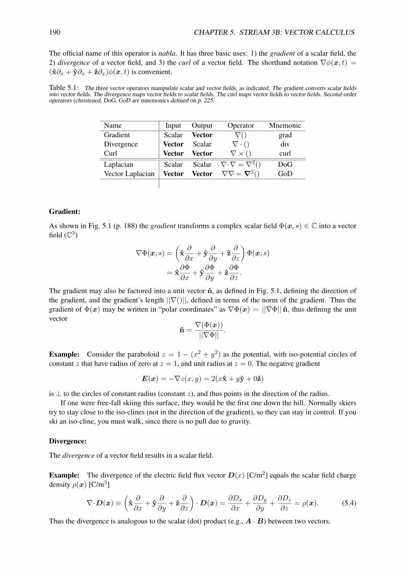
190 CHAPTER 5. STREAM 3B: VECTOR CALCULUS
The official name of this operator is nabla. It has three basic uses: 1) the gradient of a scalar field, the2) divergence of a vector field, and 3) the curl of a vector field. The shorthand notation ∇φ(x, t) =(x∂x + y∂x + z∂x)φ(x, t) is convenient.
Table 5.1: The three vector operators manipulate scalar and vector fields, as indicated. The gradient converts scalar fieldsinto vector fields. The divergence maps vector fields to scalar fields. The curl maps vector fields to vector fields. Second-orderoperators (christened, DoG, GoD are mnemonics defined on p. 225.
Name Input Output Operator MnemonicGradient Scalar Vector ∇() gradDivergence Vector Scalar ∇ · () divCurl Vector Vector ∇× () curlLaplacian Scalar Scalar ∇·∇ = ∇2() DoGVector Laplacian Vector Vector ∇∇·= ∇2() GoD
Gradient:
As shown in Fig. 5.1 (p. 188) the gradient transforms a complex scalar field Φ(x, s) ∈ C into a vectorfield (C3)
∇Φ(x, s) =(
x ∂
∂x+ y ∂
∂y+ z ∂
∂z
)Φ(x, s)
= x∂Φ∂x
+ y∂Φ∂y
+ z∂Φ∂z
.
The gradient may also be factored into a unit vector n, as defined in Fig. 5.1, defining the direction ofthe gradient, and the gradient’s length ||∇()||, defined in terms of the norm of the gradient. Thus thegradient of Φ(x) may be written in “polar coordinates” as ∇Φ(x) = ||∇Φ|| n, thus defining the unitvector
n = ∇(Φ(x))||∇Φ|| .
Example: Consider the paraboloid z = 1 − (x2 + y2) as the potential, with iso-potential circles ofconstant z that have radius of zero at z = 1, and unit radius at z = 0. The negative gradient
E(x) = −∇z(x, y) = 2(xx + yy + 0z)
is ⊥ to the circles of constant radius (constant z), and thus points in the direction of the radius.If one were free-fall skiing this surface, they would be the first one down the hill. Normally skiers
try to stay close to the iso-clines (not in the direction of the gradient), so they can stay in control. If youski an iso-cline, you must walk, since there is no pull due to gravity.
Divergence:
The divergence of a vector field results in a scalar field.
Example: The divergence of the electric field flux vector D(x) [C/m2] equals the scalar field chargedensity ρ(x) [C/m3]
∇·D(x) ≡(
x ∂
∂x+ y ∂
∂y+ z ∂
∂z
)·D(x) = ∂Dx
∂x+ ∂Dy
∂y+ ∂Dz
∂z= ρ(x). (5.4)
Thus the divergence is analogous to the scalar (dot) product (e.g.,A ·B) between two vectors.

5.1. PROPERTIES OF FIELDS AND POTENTIALS 191
Example: Recall that the voltage is the line integral of the electric field
V (a)− V (b) =∫ b
aE(x) · dx = −
∫ b
a∇V (x) · dx = −
∫ b
a
dV
dxdx, (5.5)
which is simply the fundamental theorem of calculus (p. 147). In a charge free region, this integral isindependent of the path from a to b, which is the propriety of a conservative system.
When working with guided waves (narrow tubes of flux) having rigid walls that block flow, such thatthe diameter is small compared with the wavelength (P10, p. 134), the divergence simplifies to
∇ ·D(x) = ∇rDr = 1A(r)
∂
∂rA(r)Dr(r), (5.6)
where r is the distance down the horn (range variable), A(r) is the area of the iso-response surface as afunction of range r, andDr(r) is the radial component of vectorD as a function of range r. In spherical,cylindrical and rectangular coordinates, Eq.5.6 provides the correct expression (Table 5.2, p. 214).
Properties of the divergence: The divergence is a direct measure of the flux density of the vectorfield. A vector field is said to be incompressible if the divergence of that field is zero. It is thereforecompressible when the divergence is non-zero (e.g.,∇·D(x, s) = ρ(x, s)).
Example: Compared to air, water is considered to be incompressible. The stiffness of a fluid (i.e.,the bulk modulus) is a measure of its compressibility. At very low frequencies air may be treated asincompressible (just like water), since as s→ 0,
−∇·u(x, s) = s
ηoPoP (x, s)→ 0.
The definition of compressible depends on the wavelength in the medium, so the terms must be usedwith some awareness of the frequencies being used in the analysis. As a rule of thumb, if the wavelengthλ = co/f is much larger than the size of the system, the medium may be modeled as an incompressiblefluid.
Curl:
The curl transforms a complex vector fieldH(x, s) ∈ C3 (C(x, s) ∈ C2) [A/m2].
Example: The curl of the magnetic intensity H(x, s) vector, in the frequency domain, is equal to thevector current density C(x, s):
∇×H(x, s) ≡
∣∣∣∣∣∣∣x y z∂x ∂y ∂zHx Hy Hz
∣∣∣∣∣∣∣ = C(x, s). [A/m2] (5.7)
The notation | · | indicates the determinant (Appendix A.2.1, p. 256), ∂x is shorthand for ∂/∂x andH = [Hx, Hy, Hz]T .
The curl and the divergence are both key when writing out Maxwell’s four equations. Withouta full understanding of these two differential operators (∇·,∇×), there is little hope of understandingMaxwell’s basic results, the most important equations of mathematical physics, and the starting pointfor Einstein’s relativity theories.
The curl is a measure of the rotation of a vector field. For the case of water, it would correspond tothe angular momentum, such as in a whirlpool, or with air, a tornado. A spinning top is another example,given a spinning solid body. While a gyroscope falls over if not spinning, once spinning, it can stablystand on its pointed tip. These systems are stable due to conservation of angular momentum.

192 CHAPTER 5. STREAM 3B: VECTOR CALCULUS
Example: When H = −yx + xy + 0z, ∇×H = 2z, and thus has a constant rotation; whenH = 0x + 0y + z2z, ∇×H = 0 has a curl of zero, and thus is irrotational. There are simplerules that precisely govern when a vector field is rotational versus irrotational, and compressible versusincompressible. These classes are dictated by Helmholtz’s theorem, the fundamental theorem of vectorcalculus (Eq. 5.26, p. 231).
Laplacian:
The Laplacian operator is defined as (Table 5.1) the divergence of the gradient (DoG)∇2 ≡ ∇·∇, or
∂2
∂x2 + ∂2
∂y2 + ∂2
∂x2 . (5.8)
Starting from a scalar field, the gradient produces a vector, which is then operated on by the divergenceto take the output of the gradient back to a scalar field. Thus the Laplacian transforms a scalar fieldback to a scalar field. We have seen the Laplacian before when we defined complex analytic functions(Eq. 4.15, p. 150). A second form of Laplacian (Table 5.1). is the vector Laplacian ∇2(), defined as thegradient of the divergence∇·∇() (GoD).
Example: Taking the divergence of the simple example Eq. 5.1 results in the Laplacian of the voltage
∇2Φ(x) = −Vo(δ(x)− δ(x− 1)) = 0
for 0 < x < 1. Thus this example obeys Laplace’s equation.
Example: One of the classic examples of the Laplacian is that of a voltage scalar field Φ(x) [V],which results in the electric field vector
E(x) = [Ex(x), Ey(x), Ez(x)]T = −∇Φ(x). [V/m]
When scaled by the permittivity one obtains the electric flux D = εoE [C/m2], the charge density perunit area. Here εo [F/m] is the vacuum permittivity, which is ≈ 8.85× 10⁻¹² [F/m].
Taking the divergence ofD results in the charge density ρ(x) [C/m3] at x
∇·D = ∇2Φ(x) = ρ(x).
Thus the Laplacian of the voltage, scaled by εo, results in the local charge density.
Example: Another classic example is an acoustic pressure field %(x, t) [Pa], which defines a vec-tor force density f(x, t) = −∇%(x, t) [N/m2] (Eq. 5.24, p. 202). When this force density [N/m2] isintegrated over an area, the net radial force [N] is
Fr = −∫
S∇%(x)dx. [N] (5.9)
An inflated balloon with a static internal pressure of 3 [atm], in an ambient pressure of 1 [atm] (sealevel), forms a sphere due to the elastic nature of the rubber, which acts as a stretched spring undertension. The net force on the surface of the balloon is its area times the pressure drop of 2 atm acrossthe surface. Thus the static pressure is
%(x) = 3u(ro − r) + 1, [Pa]
where u(r) is a step function of the radius r = ||x|| > 0, centered at the center of the balloon, havingradius ro.

5.1. PROPERTIES OF FIELDS AND POTENTIALS 193
Taking the gradient gives the negative1 of the radial force density (i.e., perpendicular to the surfaceof the balloon)
−fr(r) = ∇%(x) = ∂
∂r3u(ro − r) + 1 = −2δ(ro − r). [Pa]
This equation describes a static pressure that is 1 [atm] (105 [Pa]) outside the balloon and 3 [atm] inside.The net positive force density is the negative of the gradient of the static pressure.
Finally, taking the divergence of the force produces a double delta function at r = ro, namely∇2%(x) = −2δ(1)(ro − r), were 2 is the pressure drop across the balloon. If we took the thickness ofthe rubber (l [m]) into account, then∇2% = −2(δ(ro)− δ(ro − l)).
5.1.2 Laplacian operator in N dimensions
In general it may be shown that in N = 1, 2, 3 dimensions (Sommerfeld, 1949, p. 227)
∇2r P ≡ 1
rN−1∂
∂r
(rN−1∂ P
∂r
). (5.10)
For each value of N , the area A(r) = AorN−1. This will turn out to be useful when working with the
Laplacian in 1, 2, and 3 dimensions. This naturally follows from the Webster Horn Equation (Eq. 5.29,p. 204).
Example: When N = 3 (i.e., spherical geometry)
∇2r P ≡ 1
r2∂rr2∂r P (5.11)
= 1r
∂2
∂r2 r P (5.12)
resulting in the general d’Alembert solutions (Eq. 4.8 p. 156) for the spherical wave equation
P ±(r, s) = 1re∓κ(s)r
for the spherical geometry.
Exercise: Prove this last result by expanding Eq. 5.11, 5.12 using the chain rule. Solution: Expand-ing Eq. 5.11:
1r2∂rr
2∂r P = 1r2
(2r + r2∂r
)∂r P
= 2r
P r + P rr.
Expanding Eq. 5.12:
1r∂rrr P = 1
r∂r ( P + r P r)
=1r
( P r + P r + r P rr)
= 2r
P r + P rr.
1The force is pointing out, stretching the balloon.

194 CHAPTER 5. STREAM 3B: VECTOR CALCULUS
Summary: The radial component of the Laplacian in spherical coordinates (Eq. 5.11), simplifies to
∇2r%(x) = 1
r2∂
∂rr2 ∂
∂r%(x) = 1
r
∂2
∂r2 r%(x).
Since ∇2 = ∇·∇, it follows that the net force f(x) = [Fr, 0, 0]T , (Eq. 5.9) in spherical coordinates,has a radial component Fr and angular components of zero. Thus the force across a balloon may beapproximated by a delta function across the thin sheet of stretched rubber.
Example: The previous example may be extended in an interesting way to the case of a rigid hose, arigid tube, terminated on the right in an elastic medium (the above example of a balloon), for examplean automobile tire. On the far left let’s assume there is a pump injecting the fluid into the hose. Considertwo different fluids: air and water. Air may be treated as a compressible fluid, whereas water is incom-pressible. However, such a classification is a relative, being determined by the relative compliance ofthe balloon (i.e., tire) at the relatively rigid pump and hose.
This is a special case of a more general situation: When the fluid is treated as incompressible (rigid)the speed of sound becomes infinite, and the wave equation is not the best describing equation, andthe motion is best approximated using Laplace’s equation. This is the transition from short to longwavelengths, from wave propagation, with delay, to quasi-statics, having no apparent delay.
This example may be modeled as either an electrical or mechanical system. If we take the electricalanalog, the pump is a current source, injecting charge (Q) into the hose, which being rigid cannot expand(has a fixed volume). The hose may be modeled as a resistor, and the tire as a capacitor C, which fillswith charge as it is delivered via the resistor, from the pump. A capacitor obeys the same law as a springF = KV , or in electrical terms, Q = CV . Here V is the voltage, which acts as a force F , Q is thecharge, which acts like the mass of the fluid. The charge is conserved, just as the mass of the fluid isconserved, meaning they cannot be created or destroyed. The flow of the fluid is called the flux, whichis the general term for the mass or charge current. The two equations may be rewritten directly in termsof the force F, V and flow, as an electrical current I = dQ/dt of mass flux J = dM/dt, giving twoimpedance relations:
I = d
dtCV [A] (5.13)
for the electrical analog, and
J = d
dtCF [kgm/m2]. (5.14)
It is common to treat the stiffness of the balloon, which acts as a spring with compliance C (stiffnessK = 1/C), in which case the equations reduce to the same equation, in terms of an impedance Z,typically defined in the frequency domain as the ratio of the generalized force over the generalized flow
Z(s) = 1sC
[ohms].
In the case of the mechanical system Zm(s) ≡ F/J , and for the electrical system Ze(s) ≡ V/I . It isconventional to use the unit [ohms] when working with any impedance. It is convenient to use a uniformterminology for different physical situations and forms of impedance, greatly simplifying the notation.
While the two systems are very different in their physical realization, they are mathematically equiv-alent, forming a perfect analog. The formula for the impedance is typically expressed in the Laplacefrequency domain, which of course is the LT of the time variables. In the frequency domain Ohm’s lawbecomes Eq. 5.14 for the case of a spring and Eq. 5.13 for the capacitor.
The final solution of this system is solved in the frequency domain. The impedance seen by thesource is the sum of the resistance R added to the impedance of the load, giving
Z = R+ 1sC
.
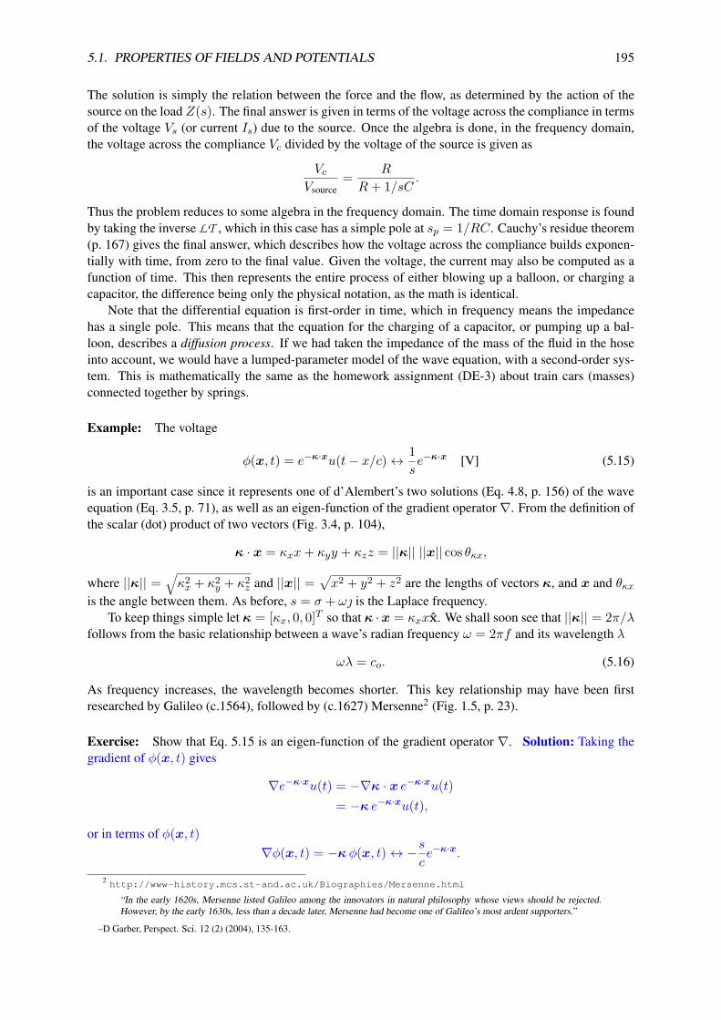
5.1. PROPERTIES OF FIELDS AND POTENTIALS 195
The solution is simply the relation between the force and the flow, as determined by the action of thesource on the load Z(s). The final answer is given in terms of the voltage across the compliance in termsof the voltage Vs (or current Is) due to the source. Once the algebra is done, in the frequency domain,the voltage across the compliance Vc divided by the voltage of the source is given as
VcVsource
= R
R+ 1/sC .
Thus the problem reduces to some algebra in the frequency domain. The time domain response is foundby taking the inverse LT , which in this case has a simple pole at sp = 1/RC. Cauchy’s residue theorem(p. 167) gives the final answer, which describes how the voltage across the compliance builds exponen-tially with time, from zero to the final value. Given the voltage, the current may also be computed as afunction of time. This then represents the entire process of either blowing up a balloon, or charging acapacitor, the difference being only the physical notation, as the math is identical.
Note that the differential equation is first-order in time, which in frequency means the impedancehas a single pole. This means that the equation for the charging of a capacitor, or pumping up a bal-loon, describes a diffusion process. If we had taken the impedance of the mass of the fluid in the hoseinto account, we would have a lumped-parameter model of the wave equation, with a second-order sys-tem. This is mathematically the same as the homework assignment (DE-3) about train cars (masses)connected together by springs.
Example: The voltage
φ(x, t) = e−κ·xu(t− x/c)↔ 1se−κ·x [V] (5.15)
is an important case since it represents one of d’Alembert’s two solutions (Eq. 4.8, p. 156) of the waveequation (Eq. 3.5, p. 71), as well as an eigen-function of the gradient operator∇. From the definition ofthe scalar (dot) product of two vectors (Fig. 3.4, p. 104),
κ · x = κxx+ κyy + κzz = ||κ|| ||x|| cos θκx,
where ||κ|| =√κ2x + κ2
y + κ2z and ||x|| =
√x2 + y2 + z2 are the lengths of vectors κ, and x and θκx
is the angle between them. As before, s = σ + ω is the Laplace frequency.To keep things simple let κ = [κx, 0, 0]T so that κ ·x = κxxx. We shall soon see that ||κ|| = 2π/λ
follows from the basic relationship between a wave’s radian frequency ω = 2πf and its wavelength λ
ωλ = co. (5.16)
As frequency increases, the wavelength becomes shorter. This key relationship may have been firstresearched by Galileo (c.1564), followed by (c.1627) Mersenne2 (Fig. 1.5, p. 23).
Exercise: Show that Eq. 5.15 is an eigen-function of the gradient operator ∇. Solution: Taking thegradient of φ(x, t) gives
∇e−κ·xu(t) = −∇κ · x e−κ·xu(t)= −κ e−κ·xu(t),
or in terms of φ(x, t)∇φ(x, t) = −κφ(x, t)↔ −s
ce−κ·x.
2 http://www-history.mcs.st-and.ac.uk/Biographies/Mersenne.html
“In the early 1620s, Mersenne listed Galileo among the innovators in natural philosophy whose views should be rejected.However, by the early 1630s, less than a decade later, Mersenne had become one of Galileo’s most ardent supporters.”
–D Garber, Perspect. Sci. 12 (2) (2004), 135-163.

196 CHAPTER 5. STREAM 3B: VECTOR CALCULUS
Thus φ(x, t) is an eigen-function of∇, having the vector eigenvalue κ. As before,∇φ is proportional tothe current since φ is a voltage, and the ratio, i.e., the eigenvalue, may be thought of as a mass, analogousto the impedance of a mass (or inductor). In general the units provide the physical interpretation of theeigenvalues and their spectra. A famous example is the Rydberg spectrum of the hydrogen atom.
Exercise: Compute n for φ(x, s) as given by Eq. 5.15. Solution: n = κ/||κ|| represents a unitvector in the κ direction.
Exercise: If the sign of κ is negative, what are the eigenvectors and eigenvalues of ∇φ(x, t)? Solu-tion:
∇e−κ·xu(t) = −κ · ∇(x)e−κ·xu(t)= −κ e−κ·xu(t).
Nothing changes other than the sign of κ. Physically this means the wave is traveling in the oppositedirection, corresponding to the forward and retrograde d’Alembert waves.
Prior to this section, we have only considered the Taylor series in one variable, such as for polyno-mials PN (x), x ∈ R (Eq.3.7 p. 72) and PN (s), s ∈ C (Eq.3.38 p. 91). The generalization from real tocomplex analytic functions led to the LT , and the hosts of integration theorems (FTCC, Cauchy I, II,III). What is in store when we generalize from one spatial variable (R) to three (R3)?
Exercise: Find the velocity v(t) of an electron in a field E. Solution: From Newton’s 2nd law,−qE = mev(t) [Nt], where me is the mass of the electron. Thus we must solve this first-order differen-tial equation to find v(t). This is easily done in the frequency domain v(t)↔ V (ω).
Role of Potentials: Note that the scalar fields (e.g., temperature, pressure, voltage) are all scalar po-tentials, summarized in Fig. 3.2 (p. 125). In each case the gradient of the potential results in a vectorfield, just as in the electric case above (Eq. 5.2).
It is important to understand the physical meaning of the gradient of a potential, which is typically ageneralized force (electric field, acoustic force density, temperature flux), which in turn generates a flow(current, velocity, heat flux). The ratio of the gradient over the flow determines the impedance.
1. Example 1: The voltage drop across a resistor causes a current to flow, as described by Ohm’slaw. Taking the difference in voltage between two points is a crude form of gradient when thefrequency f [Hz] is low, such that the wavelength is much larger than the distance between thetwo points. This is the essence of the quasi-static approximation P10 (134).
2. Example 2: The gradient of the pressure gives rise to a force density in the fluid medium (air,water, oil, etc.), which causes a flow (volume velocity vector) in the medium.
3. Example 3: The gradient of the temperature also causes a flow of heat, which is proportional tothe thermal resistance, given Ohm’s law for heat (Feynman, 1970c, p. 3-7).
4. Example 4: Nernst potential: When a solution contains charged ions, it is called an electro-chemical Nernst potentialN(x, t) (Scott, 2002). This electro-chemical field is similar to a voltageor temperature field, the gradient of which defines a virtual force on the charged ions.
Thus in the above examples there is a potential, the gradient of which is a force, which when appliedto the medium (an impedance) causes a flow (flux or current) proportional to that impedance, due to themedium. This is a very general set of concepts, worthy of some thought. In every case there is a forceand a flow. The product of the force and flow is a power, while the ratio may be modeled using 2 × 2ABCD impedance matrices (Eq. 3.7, p. 121).

5.1. PROPERTIES OF FIELDS AND POTENTIALS 197
Exercise: Show that the integral of Eq. 5.2 is an anti-derivative. Solution: The solution uses thedefinition of the anti-derivative, defined by the FTC (Eq. 4.7, p. 147):
φ(x, t)− φ(xo, t) =∫ x
xoE(x, t) · dx
= −∫ x
xo∇φ(x, t) · dx
= −∫ x
xo
(x ∂
∂x+ y ∂
∂y+ z ∂
∂z
)φ(x, t) · dx
= −∫ x
xo
(x∂φ∂x
+ y∂φ∂y
+ z∂φ∂z
)· (xdx+ ydy + zdz)
= −∫ x
xo
∂φ
∂xdx−
∫ y
yo
∂φ
∂ydy −
∫ z
zo
∂φ
∂zdz
= −∫ x
xodφ(x, t)
= −(φ(x, t)− φ(xo, t)
).
This may be verified by taking the gradient of both sides
∇φ(x, t)−>0
∇φ(xo, t) = −∇∫ x
xoE(x, t) · dx = E(x, t).
Applying the FTC (Eq. 4.7, p. 147), the anti-derivative must be φ(x, t) = Exxx + 0y + 0z. This verysame point is made by Feynman (1970c, p. 4-1, Eq. 4.28).
Given that the force on a charge is proportional to the gradient of the potential, from the aboveexercise showing that the integral of the gradient only depends on the end points, the work done inmoving a charge only depends on the limits of the integral, which is the definition of a conservativefield, but which only holds in the ideal case where E is determined by Eq. 5.2, i.e., the medium has nofriction (i.e., there are no other forces on the charge).
The conservative field: An important question is: “When is a field conservative?” A field is conser-vative when the work done by the motion is independent of the path of motion. Thus the conservativefield is related to the FTC, which states that the integral of the work only depends on the end points.
A more complete answer must await the introduction of the fundamental theorem of vector calculus,discussed in Eq. 5.26, p. 231. A few specific examples provide insight:
Example: The gradient of a scalar potential, such as the voltage (Eq. 5.2), defines the electric field,which drives a current (flow) across a resistor (impedance). When the impedance is infinite, the flow willbe zero, leading to zero power dissipation. When the impedance is lossless, the system is conservative.
Example: At audible frequencies the viscosity of air is quite small and thus, for simplicity, it may betaken as zero. However, when the wavelength is small (e.g., at 100 [kHz] λ = co/f = 345/105 =3.45 [mm]) the lossless assumption breaks down, resulting in a significant propagation loss. When theviscosity is taken into account, the field is lossy, thus the field is no longer conservative.
Example: If a temperature field is a time-varying constant (i.e., T (x, t) = To(t)), there is no “heatflux,” since∇To(t) = 0. When there is no heat flux (i.e., flux, or flow), there is no heat power, since thepower is the product of the force times the flow.

198 CHAPTER 5. STREAM 3B: VECTOR CALCULUS
Example: The force of gravity is given by the gradient of Newton’s gravitational potential (Eq. 3.1,p. 70)
F = −∇rφN(r) = − ∂
∂r
1r
= 1r2 .
Historically speaking φN (r) was the first conservative field, used to explain the elliptic orbits of theplanets around the sun. Galileo’s law says that bodies fall with constant acceleration, giving rise to aparabolic path and a time of fall proportional to t2. This behavior of falling objects directly follows fromthe Galilean potential
φG(r) = 1(r − ro)
= −ro1− r/ro
=r<ro−ro(1− r/ro + (r/ro)2 + · · · ) ≈
rroro − r,
which given the large radius ro of the earth, and the small distance of the object from the surface of theearth r − ro, is equal to the distance above the ground. Thus Galileo’s law says that the force a fallingbody sees is constant
FG = −∇rφG(r) = 1.
This can be decorated with constants to account for the actual size of the force of gravity.
Example: Galileo discovered that the height of a falling object is
r(t) = 12mGo(t− to)
2,
where m is the object’s mass and Go is the gravitational constant for the earth at its surface ro. Showthat r(t) directly follows from the potential φG = ro − r. This formula holds if you toss a ball into theair, or if you drop it from a high place. Solution: Given Galileo’s potential φG(r) = mGo(ro − r),show that the force is constant, thus that r(t) = mGo. Given Galileo’s formula for the height r(t), thevelocity is v(t) = r(t) = mGot, and the acceleration is r(t) = mGo.
Example: Find the time that it takes to fall from a distance r = L. Namely, solve r(t) = L for thetime the object takes to fall the distance L. Solution: Setting to = 0 gives t2 = 2L/mGo. Thus thetime to fall is T (L) =
√2L/mGo.
5.2 Potential solutions of Maxwell’s equations
The primary purpose for using potentials is for generating solutions to Maxwell’s equations. For ex-ample, extending Eq. 5.2 (p. 188), Maxwell’s equations may be expressed in terms of scalar and vectorpotentials. These relations are [Sommerfeld (1952, p. 146); Feynman (1970b, p. 18-10)]:
E(x, t) = −∇φ(x, t)− ∂A(x, t)∂t
, [V/m] (5.17)
and
H(x, t) = 1µo
[∇×A(x, t) + ∂D(x, t)
∂t
]. [A/m] (5.18)
Here we have extendedH(x, t) to include the electric potential term
D(x, t) = ε(x, t)E(x, t) = −ε(x, t)∇φ(x, t),
normally taken to be zero, because taking the Curl of H( t) would naturally remove any electricalpotential term, due to CoG=0.3
3“in-vacuo” εo = 8.85× 10⁻¹² [F/m2] is the capacitance, and sεo is the electric compliance-density of light. The relatedmagnetic mass-density is the permeability µo = 4π × 10−7 [H/m2] having an inductive impedance of sµo [Ω/m]. It ishelpful to think of εo as an capacitance per unit area and µo as a inductance per unit area (consistent with their units). Thespeed of light is c = 1/√εoµo = 3× 10⁸ [m/s].
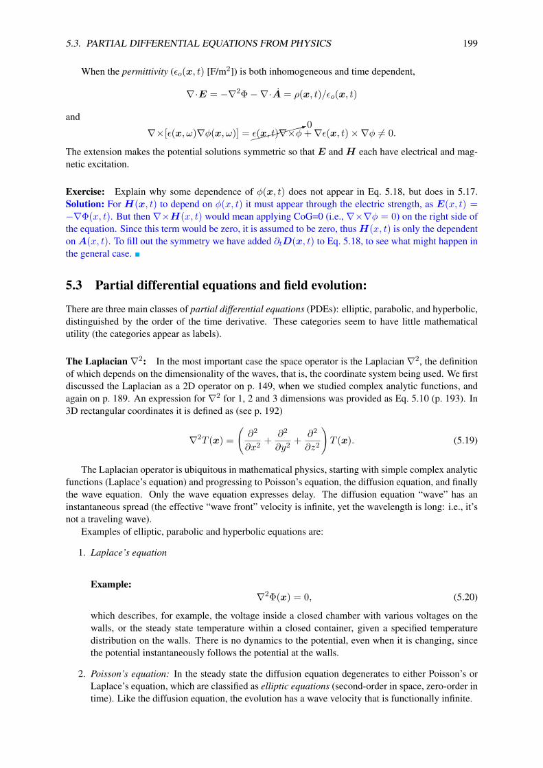
5.3. PARTIAL DIFFERENTIAL EQUATIONS FROM PHYSICS 199
When the permittivity (εo(x, t) [F/m2]) is both inhomogeneous and time dependent,
∇·E = −∇2Φ−∇·A = ρ(x, t)/εo(x, t)
and
∇×[ε(x, ω)∇φ(x, ω)] =:0
ε(x, t)∇×φ+∇ε(x, t)×∇φ 6= 0.
The extension makes the potential solutions symmetric so that E and H each have electrical and mag-netic excitation.
Exercise: Explain why some dependence of φ(x, t) does not appear in Eq. 5.18, but does in 5.17.Solution: For H(x, t) to depend on φ(x, t) it must appear through the electric strength, as E(x, t) =−∇Φ(x, t). But then ∇×H(x, t) would mean applying CoG=0 (i.e., ∇×∇φ = 0) on the right side ofthe equation. Since this term would be zero, it is assumed to be zero, thusH(x, t) is only the dependentonA(x, t). To fill out the symmetry we have added ∂tD(x, t) to Eq. 5.18, to see what might happen inthe general case.
5.3 Partial differential equations and field evolution:
There are three main classes of partial differential equations (PDEs): elliptic, parabolic, and hyperbolic,distinguished by the order of the time derivative. These categories seem to have little mathematicalutility (the categories appear as labels).
The Laplacian ∇2: In the most important case the space operator is the Laplacian ∇2, the definitionof which depends on the dimensionality of the waves, that is, the coordinate system being used. We firstdiscussed the Laplacian as a 2D operator on p. 149, when we studied complex analytic functions, andagain on p. 189. An expression for ∇2 for 1, 2 and 3 dimensions was provided as Eq. 5.10 (p. 193). In3D rectangular coordinates it is defined as (see p. 192)
∇2T (x) =(∂2
∂x2 + ∂2
∂y2 + ∂2
∂z2
)T (x). (5.19)
The Laplacian operator is ubiquitous in mathematical physics, starting with simple complex analyticfunctions (Laplace’s equation) and progressing to Poisson’s equation, the diffusion equation, and finallythe wave equation. Only the wave equation expresses delay. The diffusion equation “wave” has aninstantaneous spread (the effective “wave front” velocity is infinite, yet the wavelength is long: i.e., it’snot a traveling wave).
Examples of elliptic, parabolic and hyperbolic equations are:
1. Laplace’s equation
Example:∇2Φ(x) = 0, (5.20)
which describes, for example, the voltage inside a closed chamber with various voltages on thewalls, or the steady state temperature within a closed container, given a specified temperaturedistribution on the walls. There is no dynamics to the potential, even when it is changing, sincethe potential instantaneously follows the potential at the walls.
2. Poisson’s equation: In the steady state the diffusion equation degenerates to either Poisson’s orLaplace’s equation, which are classified as elliptic equations (second-order in space, zero-order intime). Like the diffusion equation, the evolution has a wave velocity that is functionally infinite.

200 CHAPTER 5. STREAM 3B: VECTOR CALCULUS
Example:∇2Φ(x, t) = ρ(x, t),
which holds for gravitational fields, or the voltage around a charge.
3. Fourier diffusion equation: Equation 5.22 describes the evolution of the scalar temperature T (x, t)(a scalar potential), gradients of solution concentrations (i.e., ink in water) and Brownian motion.Diffusion is first-order in time, which is categorized as parabolic (first-order in time, second-orderin space). When these equations are Laplace transformed, diffusion has a single real root, resultingin a real solution (e.g., T ∈ R). There is no wave-front for the case of the diffusion equation. Assoon as the source is turned on, the field is non-zero at every point in the bounded container.
Example:
∇2T (x, t),= Do∂T (x, t)∂t
↔ sDoT (x, s), (5.21)
which describes, for example, the temperature T (x, t) ↔ T (x, ω), as proposed by Fourier in1822, or the diffusion of two miscible liquids (Fick, 1855) and Brownian motion (Einstein, 1905).The diffusion equation is not a wave equation since the temperature wave front propagates in-stantaneously. The diffusion equation does a poor job of representing the velocity of moleculesbanging into each other, since such collisions have a mean free path, thus the velocity cannot beinfinite.
4. Two types of Wave equations:
(a) scalar wave equations: Eq. 3.3 (p. 71) describes the evolution of a scalar potential field, suchas pressure %(x, t) (sound), or the displacement of a string or membrane under tension. Thewave equation is second-order in time. When transformed into the frequency domain, thesolution has pairs of complex conjugate roots, leading to two real solutions (i.e, %(x, t ∈ R)).The wave equation is classified as hyperbolic (second-order in time and space).
(b) vector wave equations: Maxwell’s equations describe the propagation of the EM electricE(x, t) and magnetic H(x, t) field strength vectors, along with the electric D(x, t) =εoE(x, t) and magneticB(x, t) = µoH(x, t) flux vectors.
Solution evolution: The partial differential equation defines the “evolution” of the scalar field (pres-sure %(x, t)) and temperature T (x, t), or vector field (E,D,B,H), as functions of space x and time t.There are two basic categories of field evolution, diffusion and propagation.
1. Diffusion: The simplest and easiest PDE example, easily visualized, is a static4 (time invariant)scalar temperature field T (x) [°C]. Just like an impedance or admittance, a field has regions whereit is analytic, and for the same reasons, T (x, t) satisfies Laplace’s equation
∇2T (x, t) = 0.
Since there is no current when the field is static, such systems are lossless, and thus are conserva-tive.
When T (x, t) depends on time (is not static), it is described by the diffusion equation
∇2T (x, t) = κ∂
∂tT (x, t), (5.22)
a rule for how T (x, t) evolves with time from its initial state T (x, 0). Constant κ is called thethermal conductivity which depends on the properties of the fluid in the container, with sκ being
4Postulate (P3), p. 134.

5.3. PARTIAL DIFFERENTIAL EQUATIONS FROM PHYSICS 201
the admittance per unit area. The conductivity is a measure of how the heat gradients induce heatcurrents J = κ∇T , analogous to Ohm’s law for electricity.
Note that if T (x,∞) reaches steady state J = 0 as t → ∞, it evolves into a static state, thus∇2T = 0. This depends on what is happening at the boundaries. When the wall temperature of acontainer is a function of time, then so will the internal temperature continue to change, but witha delay that depends on the thermal conductivity κ.
Such a system is analogous to an electrical resistor-capacitor series circuit, connected to a battery.For example: the wall temperature (voltage across the battery) represents the potential driving thesystem. The thermal conductivity κ (the electrical resistor) is likewise analogous. The fluid (theelectrical capacitor) is being heated (charged) by the heat (charge) flux. In all cases Ohm’s lawdefines the ratio of the potential (voltage) and the flux (current). How this happens can only beunderstood once the solution to the equations has been established.
2. Propagation: Pressure and electromagnetic waves are described by a scalar potential (pressure)(Eq. 3.3, p. 71) and a vector potential (electromagnets) (Eq. 5.23, p. 229), resulting in scalar andvector wave equations.
All these partial differential equations, scalar and vector wave equations, and the diffusion equation,depend on the Laplacian∇2, which we first saw with the Cauchy-Riemann conditions (Eq. 4.15, p. 150).
The vector Taylor series: Next we expand the concept of the Taylor series of one variable, to x ∈ R3.Just as we generalized the derivative with respect to a real frequency variable ω ∈ R, to complexfrequency s = σ + ω ∈ C, here we generalize the derivative with respect to x ∈ R, to the vectorx ∈ R3.
Since the scalar field is analytic in x, it is a perfect place to start. Assuming we have carefullydefined the Taylor series 3.27 (p. 85) in one and two (Eq. 4.12, p. 149) variables, the Taylor series off(x) in x = 0 ∈ R3 may be defined as
f(x+ δx) = f(x) +∇f(x) · δx+ 12!∑k
∑l
∂2f(x)∂xk∂xl
δxkδxl + HOT. (5.23)
From this definition it is clear that the gradient is the generalization of the second term in the 1D Taylorseries expansion.
Summary: For every potential φ(x, t) there exists a force density f(x, t) = −∇φ(x, t), proportionalto the potentials, which drives a generalized flow u(x, t). If the normal component of the force andflow are averaged over a surface, the mean-force and volume-flow (i.e, volume-velocity for the acousticcase) are defined. In such cases the impedance is the net force through the surface force over the netflow, and Gauss’s law and quasi-statics (P10, p. 134) come into play (Feynman, 1970a). We call this thegeneralized impedance.
Assuming linearity (P2, p. 133), the product of the force and flow is the power, and the ratio(force/flow) is an impedance (Fig. 3.2, p. 125). This impedance statement is called either Ohm’s law,Kirchhoff’s laws, Laplace’s law, or Newton’s laws. In the simplest of cases, they are all linearized(proportional) complex relationships between a force and a flow. Very few impedance relationshipsare inherently linear over a large range of force or current, but for physically useful levels, they canbe treated as linear. Nonlinear interactions require a more sophisticated approach, typically involvingnumerical methods.
In electrical circuits it is common to define a zero potential ground point that all voltages use asthe referenced potential. The ground is a useful convention, as a simplifying rule, but it obscures thephysics, and obscures the fact that the voltage is not the force. Rather, the force is the voltage difference,

202 CHAPTER 5. STREAM 3B: VECTOR CALCULUS
referenced to the ground, which is defined as zero volts. This results in abstracting away (i.e., hiding)the difference in voltage. It seems misleading (more precisely it is wrong) to state Ohm’s law as thevoltage over the current, since Ohm’s law actually says that the voltage difference (i.e., voltage gradient)over the current defines an impedance (Kennelly, 1893).
When one measures the voltage between two points, it is a crude approximation to the gradient,based on the quasi-static approximation (P10). The pressure is also a potential, the gradient of which isa force density, which drives the volume-velocity (flow).
On p. 225 we introduce the fundamental theorem of vector calculus (aka Helmholtz’ decomposi-tion theorem), which generalizes Ohm’s law to include circulation (e.g., angular momentum, vorticityand the related magnetic effects). To understand these generalizations in flow one needs to understandcompressible and rotational fields, complex analytic functions, and a lot more history of mathematical-physics (Table 5.3, p. 223).
In summary, it is the difference in the potential (i.e., voltage, temperature, pressure) that is propor-tional to the flux. This can be viewed as a major simplification of the gradient relationship, justified bythe quasi-static assumption P10 (p. 134).
The roots of the impedance are related to the eigenmodes of the system equations.
5.4 Scalar wave equation (Acoustics)
In this section we discuss the general solution to the wave equation. The wave equation has two forms:scalar waves (acoustics) and vector waves (electromagnetics). These have an important mathematicaldistinction but a similar solution space, one scalar and the other vector. To understand the differenceswe start with the scalar wave equation.
The scalar wave equation: A good starting point for understanding PDEs is to explore the scalar waveequation (Eq. 3.3, p. 71). Thus, we shall limit our analysis to acoustics, the classic case of scalar waves.Acoustic wave propagation was first analyzed mathematically by Isaac Newton (electricity had yet to bediscovered) in his famous book Principia (1687), in which he first calculated the speed of sound basedon the conservation of mass and momentum.
Early history: The study of wave propagation begins at least as early as Huygens (ca. 1678), followedsoon after (ca. 1687) by Sir Isaac Newton’s calculation of the speed of sound (Pierce, 1981, p. 15). Theacoustic variables are the pressure
p(x, t)↔ P (x, ω)
and the particle velocity
u(x, t)↔ U(x, ω).
To obtain a wave, one must include two basic components: the stiffness of air, and its mass. Thesetwo equations shall be denoted (1) Newton’s 2nd law (F = ma) and (2) Hooke’s law (F = kx),respectively. In vector form these equations are (1) Euler’s equation (i.e., conservation of momentumdensity)
−∇p(x, t) = ρo∂
∂tu(x, t)↔ ρosU(x, s), (5.24)
which assumes the time-average density ρo to be independent of time and position x, and (2) the conti-nuity equation (i.e., conservation of mass density)
−∇·u(x, t) = 1ηoPo
∂
∂tp(x, t)↔ s
ηoPoP (x, s) (5.25)

5.5. THE WEBSTER HORN EQUATION (WHEN) 203
baffle
Baffle
balloon
Conical Horn
Dia
=2aDia
met
er=
2b
r = 0
r
y
r (range)
x = coT
Figure 5.2: Experimental setup showing a largepipe on the left terminating the wall containing a smallhole with a balloon, shown in green. At time t = 0 theballoon is pricked and a pressure pulse is released. Thebaffle on the left represents a semi-∞ long tube havinga large radius compared to the horn input diameter 2a,such that the acoustic admittance looking to the left(A/ρoco with A → ∞) is very large compared to thehorn’s throat admittance (Eq. 4.12, p. 157). At time Tthe outbound pressure pulse p(r, T ) = δ(t− x/co)/rhas reached a radius x = r − ro = coT where r = xis the location of the source at the throat of the hornand r is measured from the vertex. At the throat of thehorn V +/A+ = V −/A−.
(Pierce, 1981; Morse, 1948, p. 295). Here Po = 105 [Pa] is the barometric pressure, ηoPo is the dynamic(adiabatic) stiffness, with ηo = 1.4. Combining Eqs. 5.24 and 5.25 (removing u(x, t)) results in the 3-dimensional (3D) scalar pressure wave equation
∇2p(x, t) = 1c2o
∂2
∂t2p(x, t)↔ s2
c2o
P (x, s) (5.26)
with co =√ηoPo/ρo being the sound velocity. Because the merged equations describe the pressure,
which is a scalar field, this is an example of the scalar wave equation.
Exercise: Show that Eqs. 5.24 and 5.25 can be reduced to Eq. 5.26. Solution: Taking the divergenceof Eq. 5.24 gives
−∇·∇p(x, t) = ρo∂
∂t∇·u(x, t). (5.27)
Note that ∇·∇ = ∇2 (Table 5.1, 190). Next, substituting Eq. 5.25 into the above relation results in thescalar wave equation Eq. 5.26, since co =
√ηoPo/ρo.
5.5 The Webster horn equation
There is an important generalization of the problem of lossless plane-wave propagation in 1-dimensional(1D) uniform tubes, known as transmission line theory. As depicted in Fig. 5.2, by allowing the areaA(r) (e.g., for the conical horn A(r) = Ao(r/L)2 with L = 1 [m] and A0 ≤ 4π) of an acousti-cal waveguide (aka, horn) to vary along the range axis r (the direction of wave propagation) generalsolutions to the wave equation may be explored. Classic applications of horns include vocal tract acous-tics, loudspeaker design, cochlear mechanics, quantum mechanics (e.g., the hydrogen atom), and wavepropagation in periodic media (Brillouin, 1953).
One must be precise when defining the area A(x): The area is not the cross-sectional area of thehorn, rather it is the wave-front (iso-pressure) area, and related to Gauss’ Law, since the gradient of thepressure defines the force that drives the mass flow (aka, volume velocity).
For the scalar wave equation (Eq. 5.10, p. 193), the Webster Laplacian is
∇2r %(r, t) = 1
A(r)∂
∂r
[A(r) ∂
∂r
]%(r, t). (5.28)
The Webster Laplacian is based on the quasi-static approximation (P10: p. 134), which requires thatthe frequency lie below the critical value fc = co/2d, namely that a half wavelength be greater thanthe horn diameter d (i.e., d < λ/2).5 For the case of the adult human ear canal, d = 7.5 [mm],fc = (343/2 · 7.5)× 10−3 ≈ 22.87 [kHz].
5This condition may be written several ways, the most common being ka < 1, where k = 2π/λ and a is the horn radius.This may be expressed in terms of the diameter as 2π
λd2 < 1, or d < λ/π < λ/2. Thus d < λ/2 may be a more precise metric
by the factor π/2 ≈ 1.6. This is called the half-wavelength assumption, a synonym for the quasi-static approximation.

204 CHAPTER 5. STREAM 3B: VECTOR CALCULUS
Figure 5.3: Throat acoustical resistance rAand acoustical reactance xA , frequency char-acteristics of infinite eigen-functions of theparabolic, conical, exponential, hyperbolic andcylindrical horns, having a throat area of 1[cm2]. Note how the “critical” frequency (de-fined here as the frequency where the reactiveand real parts of the radiation impedance areequal) of the horn reduces dramatically withthe type of horn. For the uniform horn, the re-active component is zero, so there is no cutofffrequency. For the parabolic horn (1) the cutoffis around 3 kHz. For the conical horn (2) thecutoff is at 0.6 [kHz]. For the exponential horn(3) the critical frequency is around 0.18 [kHz],which is one 16th that of the parabolic horn.For each horn the cross-sectional area is de-fined as 100 [cm2] at a distance of L = 1 [m]from the throat (Olson, 1947, p. 101), (Morse,1948, p. 283).
The term on the right of Eq. 5.28, which is identical to Eq. 5.10 (p. 193), is also the Laplacian for thintubes (e.g., rectangular, spherical, and cylindrical coordinates). Thus the Webster horn “wave” equationis
1A(r)
∂
∂r
[A(r) ∂
∂r
]%(r, t) = 1
c2o
∂2
∂t2%(r, t)↔ s2
c2o
P (r, s), (5.29)
where %(r, t) ↔ P (r, s) is the acoustic pressure in Pascals [Pa] (Hanna and Slepian, 1924; Mawardi,1949; Eisner, 1967; Morse, 1948); Olson (1947, p. 101); Pierce (1981, p. 360). Extensive experimentalanalyses for various types of horns (conical, exponential, parabolic) along with a review of horn theorymay be found in Goldsmith and Minton (1924). Of special interest is Eisner (1967) due to his historysection and long list of relevant article.
The limits of the Webster horn equation: It is commonly stated that the Webster horn equation(WHEN) is fundamentally limited and thus is an approximation that only applies to frequencies muchlower than fc (Morse, 1948; Shaw, 1970; Pierce, 1981). However, in all these discussions it is assumedthat the area function A(r) is the horn’s cross-sectional area, not the area of the iso-pressure wave-front.
In the next section it is shown that this “limitation” may be avoided (subject to the f < fc quasi-static limit, P10, p. 134), making the Webster horn theory an “exact” solution for the lowest-order“plane-wave” eigen-functions of Eq. 5.29. The limiting nature of the quasi-static approximation is thatit “ignores” higher-order evanescent modes, which are naturally small since, being evanescent modesbelow their cutoff frequency, the wave number is real, thus they do not propagate (Hahn, 1941; Karal,1953). This is the same approximation that is required to define an impedance, since every eigenmodehas an impedance (Miles, 1948). This method is frequently called a modal-analysis or eigen analysis.These modes define a Hilbert “vector” space (aka, eigen-space).
As derived in Appendix G (p. 293), the acoustic variables (eigen-functions) are redefined on theiso-pressure wave-front boundary for the pressure and the corresponding volume velocity (Hanna andSlepian, 1924; Morse, 1948; Pierce, 1981). The resulting acoustic impedance is then the ratio of thepressure over the volume velocity. This approximation is valid up to the frequency where the first crossmode begins to propagate (f > fc), which may be estimated from the roots of the Bessel eigen-functions(Morse, 1948). Perhaps it should be noted that these ideas, which come from acoustics, apply equallywell to electromagnetics, or any other wave phenomena described by eigen-functions.
The best known examples of wave propagation are electrical and acoustic transmission lines. Such

5.5. THE WEBSTER HORN EQUATION (WHEN) 205
systems are loosely referred to as the telegraph or telephone equations, referring back to the early daysof their discovery (Heaviside, 1892; Campbell, 1903b; Brillouin, 1953; Feynman, 1970a). In acoustics,wave-guides are known as horns, such as the horn connected to the first phonographs from around theturn of the century (Webster, 1919). Thus the names reflect the historical development, to a time whenthe mathematics and the applications were running in close parallel.
5.5.1 Matrix formulation of WHEN
Newton’s laws of conservation of momentum (Eq. 5.24) and mass (Eq. 5.25) are modern versions ofNewton’s starting point for calculating the horn lowest-order plane-wave eigenmode wave speed.
The acoustic equations for the average pressure P (r, ω) and the volume velocity are derived inAppendix G, where the pressure and particle velocity equations (Eqs. G.4, G.6) are transformed into a2× 2 matrix of acoustical variables, average pressure P (r, ω) and volume velocity V (r, ω)
− d
dr
[P (r, ω)V (r, ω)
]=[
0 sρ0A(r)
sA(r)ηoPo
0
] [P (r, ω)V (r, ω)
]. (5.30)
DefineM(r) = ρo/A(r) and C(r) = A(r)/ηoPo (5.31)
as the per-unit-length mass and compliance of the horn (Ramo et al., 1965, p. 213). The product ofP (r, ω) and V (r, ω) define the acoustic power while their ratio defines the horns admittance admittanceY ±in (r, s), looking in the two directions (Pierce, 1981, p. 37-41).
To obtain the Webster horn pressure equation Eq. 5.29 from Eq. 5.30, take the partial derivative ofthe top equation
−∂2 P∂r2 = s
∂M(r)∂r
V + sM(r)∂V∂r
,
and then use the lower equation to remove ∂V /∂r
∂2 P∂r2 − s
∂M(r)∂r
V = s2M(r)C(r) P = s2
c2o
P .
Then use the upper equation a second time to remove V
∂2
∂r2 P + 1A(r)
∂A(r)∂r
∂
∂rP = s2
c2o
P (r, s). (5.32)
By use of the chain rule, equations of this form may be directly integrated, since
∇r P = 1A(r)
∂
∂r
[A(r) ∂
∂r
]P (r, s)
= ∂2
∂r2 P (r, s) + 1A(r)
∂A(r)∂r
P (r, s). (5.33)
This is equivalent to integration by parts, with integration factorA(r). Next we set κ(s) ≡ s2/c2o, which
later will be generalized to include visco-thermal losses (Eq. D.1, p. 279).Merging Eqs. 5.32 and 5.33 results in the Webster horn equation (WHEN) (Eq. 5.29, p. 204):
1A(r)
∂
∂rA(r) ∂
∂rP (r, s) = κ2(s) P (r, s)↔ 1
c2o
∂2
∂t2%(r, t). (5.34)
Equations having this form are known as Sturm-Liouville equations.This important class of ordinary differential equations follows from the use of separation of variables
of the Laplacian, in any (i.e., every) separable coordinate system (Morse and Feshbach, 1953, Ch. 5.1,p. 494-523). The frequency domain eigen-solutions are denoted P ±(r, s), which have a correspondingvolume velocities, denoted V ±(r, s).

206 CHAPTER 5. STREAM 3B: VECTOR CALCULUS
Summary: We transformed the 3D acoustic wave equation into acoustic variables (Eq. 5.26, p. 203) inAppendix G by the application of Gauss’s law, resulting in the 1D Webster horn equation (aka WHEN)(Eq. 5.29, p. 204), which is a non-singular Sturm-Liouville equation.6 Thus we demonstrated thatEqs. 5.26 and 5.30 reduce to to Eq. 5.34 in a horn.
6The Webster horn equation is closely related to the Schrodinger’s equation (Salmon, 1946).

5.6. EXERCISES VC-1 207
5.6 Exercises VC-1
Topic of this homework: Vector algebra and fields in R3; Gradient and scalar Laplacian operator;Definitions of Divergence and Curl; Gauss’s (divergence) & Stokes’ (Curl) LawSchwarz inequality; Quadratic forms; System postulates
Vector algebra in R3.
Definitions of the vector scalar (aka dot) A · B, cross A × B and triple product A · (B × C) maybe found in Appendix A (p. 249), where A,B,C in R3 ⊂ C3). A fourth “double-cross” (A) vectorproduct is:7
A× (B ×C) = αoB − βoC.
where αo = A ·C and βo = A ·B (Note: A× (B ×C) 6= (A×B)×C).
θ
L∗
A ·B = ||A|| ||B|| cos θ ∈ R
C = A ∧B z = ||A|| ||B|| sin θ z ∈ R
A∧B
A
B
Vector product: ⊥ AB plane
Scalar product: InAB plane
yx
z
Figure 5.4: Definitions of vectorsA,B,C (vectors in R3) used in the definition ofA ·B,A×B andA · (B×C). Thereare two algebraic vector products, the scalar (dot) product A ·B ∈ R and the vector (cross) product A×B ∈ R3. Note thatthe result of the dot product is a scalar, while the vector product yields a vector, which is⊥ to the plane containingA,B. Thisis figure 3.4 (p. 104), §3.5.
Problem # 1: Scalar product A ·B
–Q 1.1: If A = axx + ayy + azz and B = bxx + byy + bzz, write out the definition ofA ·B.
–Q 1.2: The dot product is often defined as ||A|| ||B|| cos(θ), where ||A|| =√A ·A and θ
is the angle betweenA,B. If ||A|| = 1, describe how the dot product relates to the vector B.
Problem # 2: Vector (cross) product A×B
–Q 2.1: If A = axx + ayy + azz and B = bxx + byy + bzz, write out the definition ofA×B.
7Greenberg p. 694, Eq. 8.
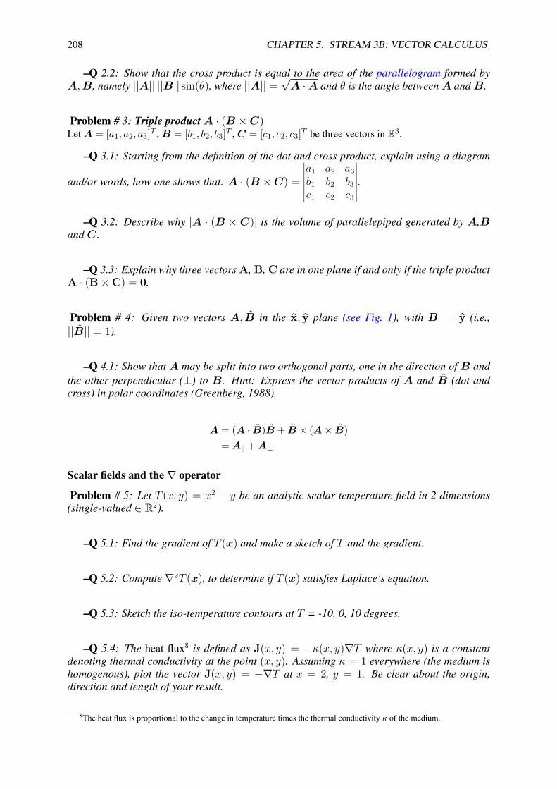
208 CHAPTER 5. STREAM 3B: VECTOR CALCULUS
–Q 2.2: Show that the cross product is equal to the area of the parallelogram formed byA,B, namely ||A|| ||B|| sin(θ), where ||A|| =
√A ·A and θ is the angle betweenA andB.
Problem # 3: Triple productA · (B ×C)LetA = [a1, a2, a3]T ,B = [b1, b2, b3]T , C = [c1, c2, c3]T be three vectors in R3.
–Q 3.1: Starting from the definition of the dot and cross product, explain using a diagram
and/or words, how one shows that: A · (B ×C) =
∣∣∣∣∣∣∣a1 a2 a3b1 b2 b3c1 c2 c3
∣∣∣∣∣∣∣.–Q 3.2: Describe why |A · (B × C)| is the volume of parallelepiped generated by A,B
and C.
–Q 3.3: Explain why three vectors A, B, C are in one plane if and only if the triple productA · (B×C) = 0.
Problem # 4: Given two vectors A, B in the x, y plane (see Fig. 1), with B = y (i.e.,||B|| = 1).
–Q 4.1: Show thatA may be split into two orthogonal parts, one in the direction ofB andthe other perpendicular (⊥) to B. Hint: Express the vector products of A and B (dot andcross) in polar coordinates (Greenberg, 1988).
A = (A · B)B + B × (A× B)= A‖ +A⊥.
Scalar fields and the∇ operator
Problem # 5: Let T (x, y) = x2 + y be an analytic scalar temperature field in 2 dimensions(single-valued ∈ R2).
–Q 5.1: Find the gradient of T (x) and make a sketch of T and the gradient.
–Q 5.2: Compute∇2T (x), to determine if T (x) satisfies Laplace’s equation.
–Q 5.3: Sketch the iso-temperature contours at T = -10, 0, 10 degrees.
–Q 5.4: The heat flux8 is defined as J(x, y) = −κ(x, y)∇T where κ(x, y) is a constantdenoting thermal conductivity at the point (x, y). Assuming κ = 1 everywhere (the medium ishomogenous), plot the vector J(x, y) = −∇T at x = 2, y = 1. Be clear about the origin,direction and length of your result.
8The heat flux is proportional to the change in temperature times the thermal conductivity κ of the medium.

5.6. EXERCISES VC-1 209
–Q 5.5: Find the vector ⊥ to ∇T (x, y), namely tangent to the iso-temperature contours.Hint: Sketch it for one (x, y) point (e.g., 2,1) and then generalize.
–Q 5.6: The thermal resistance RT is defined as the potential drop ∆T over the magnitudeof the heat flux |J|. At a single point the thermal resistance is
RT (x, y) = −∇T/|J|.
How is RT (x, y) related to the thermal conductivity κ(x, y)?
Problem # 6: Acoustic wave equation: Note: In the following problem, we will work in thefrequency domain.The basic equations of acoustics in 1 dimension are
− ∂
∂xP = ρosV and − ∂
∂xV = s
ηoPoP .
Here P (x, ω) is the pressure (in the frequency domain), V (x, ω) is the volume velocity (integral of thevelocity over the wave-front having area A), s = σ+ω, ρo = 1.2 is the specific density of air, ηo = 1.4and Po is the atmospheric pressure (i.e., 105 [Pa]) (see the handout Appendix F.2 for details). Note thatthe pressure field P is a scalar (pressure does not have direction), while the volume velocity field V is avector (velocity has direction).
We can generalize these equations to 3 dimensions using the∇ operator
−∇P = ρosV and −∇ ·V = s
ηoPoP .
–Q 6.1: Starting from these two basic equations, derive the scalar wave equation in termsof the pressure P ,
∇2P = s2
c20
P
where c0 is a constant representing the speed of sound.
–Q 6.2: What is c0 in terms of η0, ρ0, and P0?
–Q 6.3: Rewrite the pressure wave equation in the time domain, using the time derivativeproperty of the Laplace transform (e.g. dx/dt ↔ sX(s)). For your notation, define the time–domain signal using a lowercase letter, p(x, y, z, t)↔ P .
Vector fields and the∇ operator
Vector Algebra
Problem # 7: Let R(x, y, z) ≡ x(t)x + y(t)y + z(t)z:
–Q 7.1: If a, b, c are constants, what is R(x, y, z) ·R(a, b, c)?
–Q 7.2: If a, b, c are constants, what is ddt
(R(x, y, z) ·R(a, b, c))?

210 CHAPTER 5. STREAM 3B: VECTOR CALCULUS
Problem # 8: Find the divergence and curl of the following vector fields:
–Q 8.1: v = x + y + 2z
–Q 8.2: v(x, y, z) = xx + xyy + z2z
–Q 8.3: v(x, y, z) = xx + xyy + log(z)z
–Q 8.4: v(x, y, z) = ∇(1/x+ 1/y + 1/z)
Vector & scalar field identities
Problem # 9: Find the divergence and curl of the following vector fields:
–Q 9.1: v = ∇φ, where φ(x, y) = xey
–Q 9.2: v = ∇×A, where A = xx + yy + zz
–Q 9.3: v = ∇×A, where A = yx + x2y + zz
]
–Q 9.4: For any differentiable vector field V, write down two vector-calculus identities thatare equal to zero.
–Q 9.5: What is the most general form of a vector field may be expressed in, in terms ofscalar Φ and vector A potentials?
Problem # 10: Perform the following calculations. If you can state the answer without doingthe calculation, explain why.
–Q 10.1: Let v = sin(x)x + yy + zz. Find ∇ · (∇× v) Hint: Look at Lec 41 on page 83of the notes, Eq. 1.58, 59.
–Q 10.2: Let v = sin(x)x + yy + zz. Find ∇× (∇√
v · v)
–Q 10.3: Let v(x, y, z) = ∇(x+ y2 + sin(log(z)). Find ∇× v(x, y, z).

5.6. EXERCISES VC-1 211
Integral theorems
Problem # 11: Gauss’ and Stokes’ laws.
–Q 11.1: In a few words, identify the law, define what it means, and explain the followingformula: ∫
Sn · v dA =
∫V∇ · v dV.
–Q 11.2: What is the name of this formula?∫S
(∇×V) · dS =∮C
V · dR
Give one important application.
–Q 11.3: Describe a key application of the vector identity
∇× (∇×V) = ∇(∇ ·V)−∇2V.
Schwarz inequality
Problem # 12: Below is a picture of these three vectors for an arbitrary value of a and a specific a = a∗.
V + 0.5UE(α) =V−αU
|V · U |/||V ||
UE(α∗ )
=V−α∗U
V
α∗U αU
–Q 12.1: Find the value of a∗ ∈ R such that the length (norm) of E (i.e., ||E|| ≥ 0) isminimum? Hint minimize
||E||2 = E ·E = (V + aV) · (V + aU) ≥ 0 (5.1)
with respect to a.
–Q 12.2: Find the formula for ||E(a∗)||2 ≥ 0. Hint: Substitute a∗ into Eq. 5.1, and showthat this results in the Schwarz inequality
|U ·V| ≤ ||U||||V||.
Problem # 13: What is the geometrical meaning of the dot product of two vectors?
–Q 13.1: Give the formula for the dot product between two vectors. Explain the meaningbased on Fig. 12.
–Q 13.2: Write the formula for the “dot product” between two vectors: U · V in Rn inpolar form (e.g., assume the angle between the vectors is equal to θ).

212 CHAPTER 5. STREAM 3B: VECTOR CALCULUS
–Q 13.3: How is this related to the Pythagorean theorem?
–Q 13.4: Starting from ||U + V || derive the triangle inequality
||U + V|| ≤ ||U||+ ||V||.
–Q 13.5: The triangular inequality ||U+V|| ≤ ||U||+ ||V|| is true for 2 and 3 dimensions:Does it hold for 5 dimensional vectors?
Quadratic forms
A matrix that has positive eigenvalues is said to be positive-definite. The eigenvalues are real if thematrix is symmetric, so this is a necessary condition for the matrix to be positive-definite. This conditionis related to conservation of energy since the power is the voltage times the current. Given an impedancematrix
V = ZI,
the power P isP = I ·V = I · ZI,
which must be positive definite for the system to obey conservation of energy.
Problem # 14: For the following problems, consider the 2× 2 impedance matrix
Z =[2 11 4
].
–Q 14.1: Solve for the power P (i1, i2) by multiplying out the matrix equation below (which
is in quadratic form) (I ≡[i1 i2
]T)
P (i1, i2) = IT[2 11 4
]I.
–Q 14.2: Is the impedance matrix positive definite? Show your work by finding the eigen-values of the matrix Z.
–Q 14.3: Should an impedance matrix always be positive definite? Explain.
System Classification
Problem # 15: Answer the following system classification questions about physical systems,in terms of the system postulates.
–Q 15.1: Provide a brief definition of the following properties:L/NL : linear(L)/nonlinear(NL):
TI/TV : time-invariant(TI)/time varying(TV):
P/A : passive(P)/active(A):
C/NC : causal(C)/non-causal(NC):

5.6. EXERCISES VC-1 213
Re/Clx : real(Re)/complex(Clx):
–Q 15.2: Along the rows of the table, classify the following systems: In terms of a tablehaving 5 columns, labeled with the abbreviations: L/NL, TI/TV, P/A, C/NC, Re/Clx:
Category
# Case: Definition L/NL TI/TV P/A C/NC Re/Clx1 Resistor v(t) = r0 i(t)2 Inductor v(t) = Ldi
dt
3 Switch v(t) ≡
0 t ≤ 0V0 t > 0.
5 Transistor Iout = gm(Vin)7 “Resistor” v(t) = r0 i(t+ 3)8 modulator f(t) = ei2πtg(t)
–Q 15.3: Using the same classification scheme, characterize the following equations:
# Case: L/NL TI/TV P/A C/NC Re/Clx1 A(x)d
2y(t)dt2
+D(t)y(x, t) = 02 dy(t)
dt+√t y(t) = sin(t)
3 y2(t) + y(t) = sin(t)4 ∂2y
∂t2+ xy(t+ 1) + x2y = 0
5 dy(t)dt
+ (t− 1) y2(t) = iet
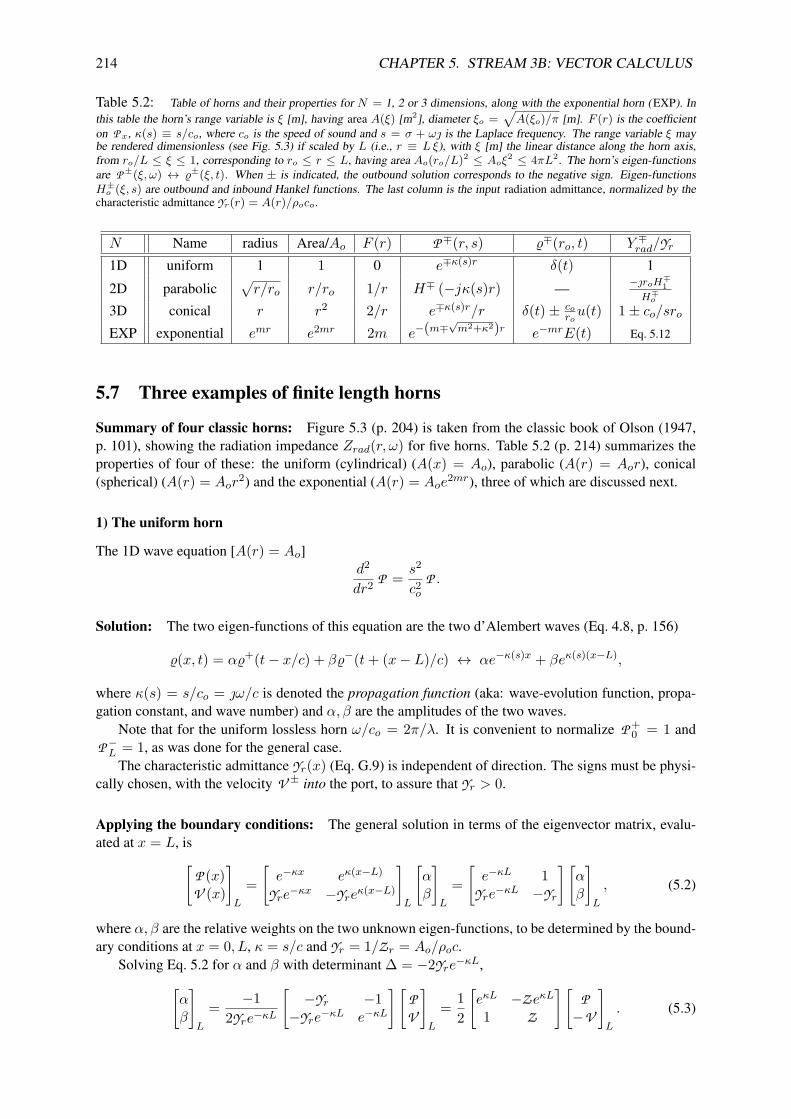
214 CHAPTER 5. STREAM 3B: VECTOR CALCULUS
Table 5.2: Table of horns and their properties for N = 1, 2 or 3 dimensions, along with the exponential horn (EXP). Inthis table the horn’s range variable is ξ [m], having area A(ξ) [m2], diameter ξo =
√A(ξo)/π [m]. F (r) is the coefficient
on P x, κ(s) ≡ s/co, where co is the speed of sound and s = σ + ω is the Laplace frequency. The range variable ξ maybe rendered dimensionless (see Fig. 5.3) if scaled by L (i.e., r ≡ Lξ), with ξ [m] the linear distance along the horn axis,from ro/L ≤ ξ ≤ 1, corresponding to ro ≤ r ≤ L, having area Ao(ro/L)2 ≤ Aoξ
2 ≤ 4πL2. The horn’s eigen-functionsare P±(ξ, ω) ↔ %±(ξ, t). When ± is indicated, the outbound solution corresponds to the negative sign. Eigen-functionsH±o (ξ, s) are outbound and inbound Hankel functions. The last column is the input radiation admittance, normalized by thecharacteristic admittance Yr(r) = A(r)/ρoco.
N Name radius Area/Ao F (r) P ∓(r, s) %∓(ro, t) Y ∓rad/Yr1D uniform 1 1 0 e∓κ(s)r δ(t) 1
2D parabolic√r/ro r/ro 1/r H∓ (−jκ(s)r) — −roH∓1
H∓o3D conical r r2 2/r e∓κ(s)r/r δ(t)± co
rou(t) 1± co/sro
EXP exponential emr e2mr 2m e−(m∓√m2+κ2)r e−mrE(t) Eq. 5.12
5.7 Three examples of finite length horns
Summary of four classic horns: Figure 5.3 (p. 204) is taken from the classic book of Olson (1947,p. 101), showing the radiation impedance Zrad(r, ω) for five horns. Table 5.2 (p. 214) summarizes theproperties of four of these: the uniform (cylindrical) (A(x) = Ao), parabolic (A(r) = Aor), conical(spherical) (A(r) = Aor
2) and the exponential (A(r) = Aoe2mr), three of which are discussed next.
1) The uniform horn
The 1D wave equation [A(r) = Ao]d2
dr2 P = s2
c2o
P .
Solution: The two eigen-functions of this equation are the two d’Alembert waves (Eq. 4.8, p. 156)
%(x, t) = α%+(t− x/c) + β%−(t+ (x− L)/c) ↔ αe−κ(s)x + βeκ(s)(x−L),
where κ(s) = s/co = ω/c is denoted the propagation function (aka: wave-evolution function, propa-gation constant, and wave number) and α, β are the amplitudes of the two waves.
Note that for the uniform lossless horn ω/co = 2π/λ. It is convenient to normalize P +0 = 1 and
P −L = 1, as was done for the general case.The characteristic admittance Yr(x) (Eq. G.9) is independent of direction. The signs must be physi-
cally chosen, with the velocity V ± into the port, to assure that Yr > 0.
Applying the boundary conditions: The general solution in terms of the eigenvector matrix, evalu-ated at x = L, is[
P (x)V (x)
]L
=[e−κx eκ(x−L)
Yre−κx −Yreκ(x−L)
]L
[αβ
]L
=[e−κL 1
Yre−κL −Yr
] [αβ
]L
, (5.2)
where α, β are the relative weights on the two unknown eigen-functions, to be determined by the bound-ary conditions at x = 0, L, κ = s/c and Yr = 1/Zr = Ao/ρoc.
Solving Eq. 5.2 for α and β with determinant ∆ = −2Yre−κL,[αβ
]L
= −12Yre−κL
[−Yr −1
−Yre−κL e−κL
] [PV
]L
= 12
[eκL −Z eκL
1 Z
] [P−V
]L
. (5.3)

5.7. 3 EXAMPLES OF HORNS 215
In the final step we swapped all the signs, including on V , and moved Zr = 1/Yr inside the matrix.We may uniquely determine these two weights given the pressure and velocity at the boundary
x = L, which is typically determined by the load impedance ( P L/V L).The weights may now be substituted back into Eq. 5.2 to determine the pressure and velocity ampli-
tudes at any point 0 ≤ x ≤ L.[PV
]x
= 12
[e−κx eκ(x−L)
Yre−κx −Yreκ(x−L)
]x
[eκL −Z eκL
1 Z
] [P−V
]L
. (5.4)
Setting x = 0 and multiplying these out gives the final transmission matrix[PV
]0
= 12
[eκL + e−κL Zr(eκL − e−κL)
Yr(eκL − e−κL) eκL + e−κL
]x
[P−V
]L
. (5.5)
Note the diagonal terms are cosh κL and off-diagonal terms are sinh κL.Applying the last boundary condition, we evaluate Eq. 5.3 to obtain the ABCD matrix at the input
(x = 0) (Pipes, 1958) [PV
]0
=[
cosh κL Zr sinh κLYr sinh κL cosh κL
] [P−V
]L
. (5.6)
Note that the determinant is 1, thus the system is reciprocal.
Exercise: Evaluate this expression in terms of the load impedance.Solution: Since Zload = −P L/V L,
PV 0
= Zload cosh κL− Zr sinh κLZloadYr sinh κL− cosh κL (5.7)
Impedance matrix: Expressing Eq. 5.6 as an impedance matrix gives (algebra required)[P o
P L
]= Zr
sinh(κL)
[cosh(κL) 1
1 cosh(κL)
] [V o
V L
].
Exercise: Write out the short-circuit (V L = 0) input impedance Zin(s) for the uniform horn. Solu-tion:
Zin(s) = PoVo
= Zrcosh κLsinh κL = Zr tanh κL|VL=0 .
Input admittance Yin: Given the input admittance of the horn, it is possible to determine if it is uni-form, without further analysis. Namely, if the horn is uniform and infinite in length, the input admittanceat x = 0 is
Yin(x = 0, s) ≡ V (0, ω)P (0, ω) = Yr,
since α = 1 and β = 0. That is, for an infinite uniform horn, there are no reflections.When the uniform horn is terminated with a fixed impedance Zr at x = L, one may substitute
pressure and velocity measurements into Eq. 5.3 to find α and β, and given these, one may calculate thepressure reflectance at x = L (Eq. 3.16, p. 102)
ΓL(s) = β
α= P (L, ω)− ZrV (L, ω)
P (L, ω) + ZrV (L, ω) = ZL − Zr
ZL + Zr
given sufficiently accurate measurements of the throat pressure P (0, ω), velocity V (0, ω), and the char-acteristic impedance of the input Zr = ρoc/A(0).

216 CHAPTER 5. STREAM 3B: VECTOR CALCULUS
2) Conical horn
Using the conical horn area A(r) ∝ r2 in Eq. 5.29, p. 204 [or Eq. 5.30 (p. 205)] results in the sphericalwave equation
P rr(r, ω) + 2r
P r(r, ω) = κ2 P (r, ω). (5.8)
Radiation admittance for the conical horn: The conical horn’s acoustic input admittance Yin(r, s)at any location r is found by dividing Eq. G.4 (p. 293) by P (r, s)
Y ±in (r, s) = V ±
P ±= −A(r)
sρo
d
drln P ±(r, s) (5.9)
= Yr(r)[1± co
sr
]↔ A(r)
ρoco
(δ(t− r/co)±
coru(t− r/co)
). (5.10)
Note how the pressure pulse is delayed by r/co due to e−κ(s)r, as it travels down the horn. As the areaof the horn increases, the pressure decreases as 1/r = 1/
√A(r). This results in the uniform back-flow
c0u(t)/r due to conservation of mass and the characteristic admittance Yr(r) variation with r.
3) Exponential horn: If we define the area as A(r) = e2mr, the eigen-functions of the horn are
P ±(r, ω) = e−mre∓j√ω2−ω2
c r/c, (5.11)
which may be shown by the substitution of P±c (r, ω) into Eq. 5.29 (p. 204), with A(r) = e2mr.This case is of special interest because the radiation impedance is purely reactive below the horn’s
cutoff frequency (ω < ωc = mco), as may be seen from curves 3 and 4 of Fig. 5.3 (p. 204). As a result,no energy can radiate from an open horn for ω < ωc because
κ(s) = −m±
co
√ω2 − ω2
c
is purely real (this is the case of non-propagating evanescent waves).Using Eq. 4.12 (p. 157) the input admittance is
Y ±in (x, s) = −A(x)sρo
(m±
√m2 + κ2
)x. (5.12)
Kleiner (2013) gives an equivalent expression for Yin(x, ω) having area S(x) = emx
Yin(x, ω) = S(x)ωρ
[m
2 +
√4ω2 − (mc)2
2c
],
and impedance
Zin(r, ω) = ρc
ST
ωcω
+
√1−
(ωcω
)2 ,
where ωc(r) is the cutoff frequency.One may use expansions of A(r) in a Fourier-like exponential series along with superposition, to
find the general solution for an arbitrary analytic A(r).

5.7. 3 EXAMPLES OF HORNS 217
5.7.1 Solution methods
Two distinct mathematical techniques are used to describe physical systems: partial differential equa-tions (PDEs) and lumped parameter models (i.e., quasi-statics) (Ramo et al., 1965). We shall describeboth these methods for the case of the scalar wave equation.
1. Separable coordinate systems: Classically PDEs are solved by separation of variables. Morse(1948, p. 296-7) shows this method is limited to a few coordinate systems, such as rectangular,cylindrical and spherical coordinates. Even a slight deviation from separable specific coordinatesystems represents a major barrier toward further analysis and understanding, blocking insightinto more general cases. Separable coordinate systems have a high degree of symmetry. Note thatthe solution of the wave equation is not tied to a specific coordinate system.
2. Sturm-Liouville methods and eigenvectors: When the coordinate system is separable the re-sulting PDEs are always a Sturm-Liouville equations, an important special class of differentialequations. Sturm-Liouville equations are solved by finding their eigen-functions. Webster horntheory (Webster, 1919; Morse, 1948; Pierce, 1981) is a generalized Sturm-Liouville equation,which adds physics, in the form of the horn’s area-function.
The Webster equation side-steps the seriously limiting problem of separation of variables, bymaking it possible to use the alternative quasi-static solution, by ignoring high-frequency higherorder evanescent modes. This is essentially a 1-dimensional lowpass approximation of the waveequation.
Mathematics provides rigor, while physics provides understanding. While both are important, itis the physical applications that make a theory useful.
3. Lumped-element method: As previously described on p. 121, a system may be represented interms of lumped elements, such as electrical inductors, capacitors and resistors, or their mechanicalcounterparts, masses, springs and dash-pots. Such systems are represented by 2× 2 transmission-matrices in the s (i.e., Laplace) domain (train problem, Exercises DE3, p. 184).
When the system of lumped element networks contains only resistors and capacitors, or resistorsand inductors, the system does not support waves, and is related to the diffusion equation in itssolution. Depending on the elements in the system of equations, there can be an overlap betweena diffusion process and scalar waves, represented as transmission lines, both modeled as lumpednetworks of 2×2 matrices (Eq. 3.7, p. 121) (Campbell, 1922; Brillouin, 1953; Ramo et al., 1965).Quasi-static methods provide band-limited solutions below a critical frequency fc (where a halfwavelength approaches the element spacing) for a much wider class of geometries, by avoidinghigher-order, high-frequency cross-modes. Examples are given in Fig. 3.9 (p. 126) and DE3,Problem 2 (p. 184),
When the wavelength is longer than the physical distance between the elements, the approxi-mation is mathematically equivalent to a transmission line. As the frequency increases, and thewavelength becomes equal to (f = fc = co/2d), the quasi-static (lumped element) model breaksdown. This is under the control of the modeling process, as elements must be added to representhigher frequencies (shorter wavelengths). If the nature of the solution at high frequencies (f > fc)is desired, one must add more sections, thereby increasing fc. For many (perhaps most) problems,lumped elements are easy to use, and accurate Brillouin (1953); Ramo et al. (1965) as long as youdon’t violate the upper frequency limit.
5.7.2 Eigen-function solutions %±(r, t) of the Webster horn equation
Because the wave equation (Eq. 5.26) is 2nd order in time, there are two causal independent eigen-function solutions of the homogeneous (i.e., un-driven) Webster horn equation: an outbound (right-traveling) %+(r, t) and an inbound (left-traveling) %−(r, t) wave. These causal eigen-solutions may be

218 CHAPTER 5. STREAM 3B: VECTOR CALCULUS
Laplace transformed into the frequency-domain
%±(r, t)↔ P ±(r, s) =∫ ∞
0−%±(r, t)e−stdt.
They may be normalized so that P ±(ro, s) = 1, where ro is the source excitation reference point.Every eigen-functions depends on an area function A(r) (Eq. 5.29, p. 204). In theory then, given
one it should be possible to find the other. This is known as the inverse problem, which is generallybelieved to be an unsolved problem. For example, given the eigenvalues λk, how does one determinethe corresponding area function A(r)?
Because the characteristic impedance Yr(r) of the wave in the horn changes with location, theremust be local reflections due to these area variations. Thus there are fundamental relationships betweenthe area change dA(r)/dr, the horn’s eigen-functions P ±(r, s), eigenmodes and input impedance.
Complex vs. real frequency: We shall continue to maintain the distinction that functions of ω areFourier transforms and causal functions of Laplace frequency s correspond to Laplace transforms, whichare necessarily complex analytic in s in the right half-plane (RHP) region of convergence (RoC). Thisdistinction is critical since we typically describe impedance Z(s), and admittance Y (s), as complexanalytic functions in s, in terms of their poles and zeros. The eigen-functions P ±(r, s) of Eq. 5.29 arealso causal complex analytic functions of s.
Plane-wave eigen-function solutions: Huygens (1690), three years after Newton’s publication ofPrincipia, was the first to gain insight into wave propagation, today known as “Huygens’s principle.”While his concept showed a deep insight, we now know it was seriously flawed, as it ignored the back-ward traveling wave (Miller, 1991). In 1747 d’Alembert published the first correct solution for theplane-wave scalar wave equation
%(x, t) = f(t− x/co) + g(t+ x/co), (5.13)
where f(·) and g(·) are general functions of their argument. Why this is the solution may be easilyshown by use of the chain rule, by taking partials with respect to x and t.
In terms of the physics, d’Alembert’s general solution describes two arbitrary wave-forms f(·), g(·)traveling at a speed co, one forward and one reversed. Thus his solution is quite easily visualized.
Exercise: By the use of the chain rule, prove that d’Alembert’s formula satisfies the 1D wave equation.Solution: Taking a derivative with respect to t and r gives
• ∂t%(r, t) = −cof ′(r − cot) + cog′(r + cot)
• ∂r%(r, t) = f ′(r − cot) + g′(r + cot),
and a second derivative gives
• ∂tt%(r, t) = c2of′′(r − cot) + c2
og′′(r + cot)
• ∂rr%(r, t) = f ′′(r − cot) + g′′(r + cot).
From these last two equations we have the 1D wave equation
∂rr%(r, t) = 1c2o
∂tt%(r, t),
having solutions Eq. 5.13.
5.8. INTEGRAL DEFINITIONS OF∇(), ∇·() AND ∇×() 219
Example: Assuming f(·), g(·) are δ(·), find the Laplace transform of the solution corresponding tothe uniform horn A(x) = 1.
Solution: Using Table C.3 (p. 272) of Laplace transforms on Eq. 5.13 gives
%(x, t) = δ(t− x/co) + δ(t+ x/co)↔ e−sx/co + esx/co . (5.14)
Note that the delay To = ±x/co depends on the range x.
3D d’Alembert spherical eigen-functions: The d’Alembert solution generalizes to spherical wavesby changing the area function of Eq. 5.29 to A(r) = Aor
2 (See Eq. 5.10, p. 193 and Table 5.2, p. 214).The wave equation then becomes
∇2r%(r, t) = 1
r
∂2
∂r2 r%(r, t) = 1c2o
∂2
∂t2%(r, t).
Multiplying by r results in the general spherical (3D) d’Alembert wave equation solution
%(r, t) = f(t− r/co)r
+ g(t+ r/co)r
for arbitrary wave-forms f(·) and g(·). These are the eigen-functions for the spherical scalar waveequation.
5.8 Integral forms of∇(), ∇·() and∇×()The vector wave equation describes the evolution of a vector field, such as Maxwell’s electric field vectorE(x, t). When these fields are restricted to a one-dimensional domain they are known as guided wavesconstrained by wave guides.
These equations use thee differential vector operators, the gradient, divergence and the curl. Thereare two forms of definitions for each of these three operators: differential and integral. The integralform provides a more intuitive view of the operator, which in the limit converges to the differentialform. Following a discussion of the gradient, divergence and curl integral operators, these two forms arediscussed.
In addition there are three fundamental vector theorems: Gauss’s law (divergence theorem), Stokes’slaw (curl theorem) and Helmholtz’s decomposition theorem. Without the use of these very fundamentalvector calculus theorems, Maxwell’s equations cannot be understood.
5.8.1 Gradient: E = −∇φ(x)
As shown in Fig. 5.1 (p. 188) the gradient maps R1 7→∇
R3. The gradient is defined as the unit-normal n,
weighted by the potential φ(x), averaged over a closed surface S
∇φ(x) ≡ limS ,V→0
∫S φ(x) n dS
V
[V/m] (5.15)
having area S and volume V , centered at x (Greenberg, 1988, p. 773).9 Here n is a dimensionless unitvector, perpendicular to the surface S
n = ∇φ‖∇φ‖
.
The dimensions of Eq. 5.15 are in the units of the potential times the area, divided by the volume, asneeded for a gradient (e.g., [V/m]). The units are potential-dependent. If φ were temperature, the unitswould be [deg/m].
9Further discussions are on pages Greenberg (1988, pp. 778, 791, 809).

220 CHAPTER 5. STREAM 3B: VECTOR CALCULUS
Exercise: Justify the units of Eq. 5.15. Solution: The units depend on φ per unit length. If φ isvoltage, then the gradient has units of [V/m]. Under the limit d|S |/||S || must have units of m−1.
The natural way to define the surface and volume is to place the surface on the iso-potential surfaces,forming either a cube or pill-box shaped volume. As the volume ||S || goes to zero, so must the area |S |.One must avoid irregular volumes where the area is finite as the volume goes to zero (Greenberg, 1988,footnote p. 762).
A well-known example is the potential
φ(x, y, z) = Q
εo√x2 + y2 + z2 = Q
εoR[V]
around a point charge Q [SI Units of Coulombs]. The constant εo is the permittivity [F/m2]. A secondwell-known example is the acoustic pressure potential around an oscillating sphere, which has the sameform (Table 5.2, p. 214).
How does this work? To better understand what Eq. 5.15 means, consider a three-dimensional Taylorseries expansion of the potential in x about the limit point xo
φ(x) ≈ φ(xo) +∇φ(x) · (x− xo) + HOT.
We could define the gradient using this relationship as
∇φ(xo) = limx→xo
φ(x)− φ(xo)x− xo
.
For this definition to apply, xmust approach xo along n. To compute the higher order terms (HOT) oneneeds the Hessian matrix.10
The natural way to define a surface |S | is to take find the iso-potential contours. The gradient is inthe direction of maximum change in the potential, thus perpendicular to the iso-potential contours. Thesecret to the integral definition is in taking the limit. As the volume ||S || shrinks to zero, the HOT termsare small, and the integral reduces to the first-order term in the Taylor expansion since the constant termintegrates to zero. Such a construction was used in the proof of the Webster horn equation (G, p. 293;Fig. G.1, p. 294).
The problem with Eq. 5.15 is that it is recursive since n is based on the gradient and is the kernel ofthe integral. Thus the integral definition of the gradient is based on the gradient itself. Equation 5.15 isactually a statement of the mean value theorem for the gradient.
5.8.2 Divergence: ∇·D = ρ [C/m3]
As briefly summarized by Eq. 5.4 on p. 190, the definition of the divergence at x = [x, y, z]T is
∇·D(x, t) ≡ [∂x, ∂y, ∂z] ·D(x, t) =[∂Dx
∂x+ ∂Dy
∂y+ ∂Dz
∂z
](x, t) = ρ(x, t),
which maps R3 7→∇·
R1.
5.8.3 Divergence and Gauss’s law
Like the gradient, the divergence of a vector field may be defined as the surface integral of a compressiblevector field, as a limit as the volume, enclosed by the surface, goes to zero. As for the case of the gradient,for this definition to make sense, the surface S must be closed, defining volume V . The difference is
10Hi,j = ∂2(x)φ/∂xi∂xj , which will exist if the potential is analytic in x at xo.

5.8. INTEGRAL DEFINITIONS OF∇(), ∇·() AND ∇×() 221
S Surface (closed)
Tangent plane
ρenc Charge
n ⊥ dS
Volume V
∇·D ≡ limV ,S→0
∫∫S n ·D dS
V
[C/m3]
Q enc =∫∫
Sn ·D dS
=∫∫∫
Vρenc dV [C]
Figure 5.5: The first equation is the integral definition of the divergence of D as an integral over the closed surface S ofthe normal component ofD, in the limit as the surface and volume shrink to 0. The second equation states the enclosed chargeQ enc in terms of the surface integral of the normal component of D. The third equation gives the charge enclosed in terms ofa volume integral over the enclosed charge density ρenc.
that the surface integral is over the normal component of the vector field being operated on (Greenberg,1988, p. 762-763)
∇·D = limV ,S→0
∫S D · n dS
V
= ρenc(x, y, z). [C/m3] (5.16)
As with the case of the gradient we have defined the surface as S , its area as S and the volume within asV . It is a necessary condition that as the area S goes to zero, so does the volume V .
As before, n is a unit vector normal to the surface S , which depends on the gradient. The limit, asthe volume and surface simultaneously go to zero, defines the total flux across the surface. Thus thesurface integral is a measure of the total flux ⊥ to the surface. It is helpful to compare this formula withthat for the gradient Eq. 5.15.
Gauss’s law: The above definitions resulted in Gauss’s Law, a major breakthrough in vector calculus.As summarized by Feynman (1970c, p. 13-2):
The current leaving the closed surface S equals the rate of the charge leaving that volumeV , defined by that surface.
For the electrical case this is equivalent to the observation that the total flux across the surface isequal to the net charge enclosed by the surface. Since the volume integral over charge density ρ(x, y, z)is total charge enclosed Qenc,
Qenc =∫∫∫
V∇·D dV =
∫∫SD ·n dS . [C] (5.17)
When the surface integral over the normal component of D(x) is zero, the total charge is zero. If thereis only positive (or negative) charge inside the surface, ∇·D = ρ(x) = 0 charge density must also bezero.
Taking the derivative with respect to time gives the total current, normal to the surface:
Ienc =∫∫
SD ·n dS = Qenc =
∫∫∫Vρenc dV . [A] (5.18)
Of course to define a volume, the surface must be closed, a necessary condition for Gauss’s law. Thisreduces to a common-sense summary that can be grasped intuitively.

222 CHAPTER 5. STREAM 3B: VECTOR CALCULUS
n ⊥ dS
Tangent planeS Surface (open)
B Boundarydl
∇×H ≡ limB ,S→0
∫∫S n×H dS
S
[A/m2]
Ienc =∫∫
S(∇×H) ·n dS =
∮BH ·dl [A]
Figure 5.6: The integral definition of the curl is related to that of the divergence (Eq. 5.16) as an integration over the tangentto the surface, except: (1) the curl is defined as the cross product n ×H [A/m2], of nwith the current density H, and (2) thesurface is open, leaving a boundary B along the open edge. As with the divergence, which leads to Gauss’s law, this definitionleads to a second fundamental theorem of vector calculus: Stokes’s law (aka the curl theorem).
5.8.4 Integral definition of the curl: ∇×H = C
As briefly summarized on page 191, the differential definition of the curl maps R3 7→∇×
R3. The curl of
the magnetic field strengthH(x) is the current density C = σE + D
∇×H ≡
∣∣∣∣∣∣∣x y z∂x ∂y ∂zHx Hy Hz
∣∣∣∣∣∣∣ = C [A/m2].
Curl and Stokes’s law: As in the cases of the gradient and divergence, the curl also may be written inintegral form, allowing for the physical interpretation of its meaning:
The surface integral definition of∇×H = C [A/m2], where the current densityC is ⊥ tothe rotation plane ofH .
Stokes’s law states that the open surface integral over the normal component of the curl of themagnetic field strength (n · ∇×H [A/m2]) is equal to the line integral
∮B H · dl along the boundary B .
As summarized in Fig. 5.6, Stokes’s law is
Ienc =∫∫
S(∇×H) ·n dS [A]
=∫∫
SC ·n dS
=∮
BH ·dl, [A]
(5.19)
namely
The line integral of H along the open surface’s boundary B is equal to the total currentenclosed Ienc .
In many texts the normalization (denominator under the integral) is a volume V (e.g., Greenberg(1988, p. 778,823-4)). However because the surface is open, this volume does not exist (when defining avolume the a surface must be closed). The definition must hold even in the limit when the curved surfaceS degenerates to a plane, with the boundary B enclosing S . In this limit there is no volume.
To resolve this problem, we have taken the normalization to be the surface S . Note that in the limitB → 0, the limiting definition is independent of any curvature, since the integral is over the normalcomponent ofH (i.e., n ⊥H(x, t)). The net flux is independent of the curvature of S as B → 0.

5.8. INTEGRAL DEFINITIONS OF∇(), ∇·() AND ∇×() 223
Summing it up: Since integration is a linear process (sums of smaller elements), one may tile (tessel-late) the surface, breaking it up into smaller surfaces and their boundaries, the sum of which is equal tothe integral over the original boundary. This is an important concept which leads to the proof of Stokes’slaw.
Table 5.1 (p. 190) provides a description of the three basic integration theorems, along with theirmapping domains. The integral formulations of Gauss’s and Stokes’s laws use n ·D and H × n in theintegrands. The key distinction between the two laws naturally follows from the properties of the scalar(A ·B) and vector (A×B) products, as discussed in Fig. 3.4, p. 104. To fully appreciate the differencesbetween Gauss’s and Stokes’s laws, these two types of vector products must be mastered.
Paraphrasing Feynman (1970c, 3-12),
1. Φ2 = Φ1 +∫ 2
1 ∇Φ · dS
2.∮D · n dS =
∮∇·D dV
3.∮
B E · dl =∮
S (∇×E) · n dS
5.8.5 Helmholtz’s decomposition
We must now rethink everything defined above, in terms of the two types of vector fields, that decom-pose every analytic vector field (Table 5.3). The irrotational field is defined as one that is “curl free.”An incompressible field is one that is “divergence free.” According to Helmholtz’s decomposition, ev-ery analytic vector field may be decomposed into independent rotational and compressible components(Helmholtz, 1978). Another name for Helmholtz decomposition is the fundamental theorem of vectorcalculus (FTVC); Gauss’s and Stokes’s theorems,11 along with Helmholtz’s decomposition form thethree key fundamental theorems of vector calculus. Portraits of Helmholtz and Kirchhoff are providedin Fig. 5.8.
Table 5.3: The four possible classifications of scalar and vector potential fields: rotational/irrotational and compressible/in-compressible. Rotational fields are generated by the vector potential (e.g., A(x, t)), while compressible fields are generatedby the scalar potentials (e.g., voltage φ(x, t), velocity ψ, pressure %(x, t) or temperature T (x, t)).
Field: Compressible Incompressiblev(x, t) ∇·v 6= 0 ∇·v = 0Rotational v = ∇φ+∇×ω v = ∇×w∇×v 6= 0 Vector wave Eq. (EM) Lubrication theory
∇2v = 1c2 v Boundary layers
Irrotational Acoustics StaticsConservative v = ∇ψ ∇2φ = 0∇×v = 0 ∇2%(x, t) = 1
c2 %(x, t) Laplace’s Eq. (c→∞)
A magnetic solenoidal field is a uniform flux field Bz(x) that is generated by a solenoidal coil,and to an excellent approximation, is uniform inside the coil, making it similar to that of a permanentmagnet. As a result, the divergence of a solenoidal field is, to a good approximation, zero, making itincompressible (∇·= 0) and rotational (∇×6= 0).
I recommend you know this term, since it is widely used, but suggest the preferred terms are incom-pressible and rotational. Strictly speaking, the term “solenoidal field” only applies to a magnetic fieldproduced by a solenoid, making the term specific to that case.
11The theorems are integral relations. The laws physical relationships which follow from the theorems.
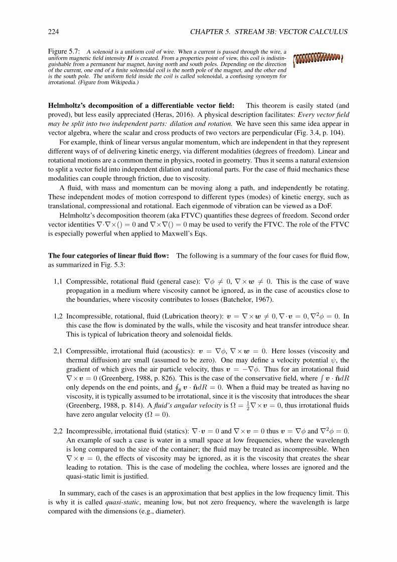
224 CHAPTER 5. STREAM 3B: VECTOR CALCULUS
Figure 5.7: A solenoid is a uniform coil of wire. When a current is passed through the wire, auniform magnetic field intensity H is created. From a properties point of view, this coil is indistin-guishable from a permanent bar magnet, having north and south poles. Depending on the directionof the current, one end of a finite solenoidal coil is the north pole of the magnet, and the other endis the south pole. The uniform field inside the coil is called solenoidal, a confusing synonym forirrotational. (Figure from Wikipedia.)
Helmholtz’s decomposition of a differentiable vector field: This theorem is easily stated (andproved), but less easily appreciated (Heras, 2016). A physical description facilitates: Every vector fieldmay be split into two independent parts: dilation and rotation. We have seen this same idea appear invector algebra, where the scalar and cross products of two vectors are perpendicular (Fig. 3.4, p. 104).
For example, think of linear versus angular momentum, which are independent in that they representdifferent ways of of delivering kinetic energy, via different modalities (degrees of freedom). Linear androtational motions are a common theme in physics, rooted in geometry. Thus it seems a natural extensionto split a vector field into independent dilation and rotational parts. For the case of fluid mechanics thesemodalities can couple through friction, due to viscosity.
A fluid, with mass and momentum can be moving along a path, and independently be rotating.These independent modes of motion correspond to different types (modes) of kinetic energy, such astranslational, compressional and rotational. Each eigenmode of vibration can be viewed as a DoF.
Helmholtz’s decomposition theorem (aka FTVC) quantifies these degrees of freedom. Second ordervector identities∇·∇×() = 0 and∇×∇() = 0 may be used to verify the FTVC. The role of the FTVCis especially powerful when applied to Maxwell’s Eqs.
The four categories of linear fluid flow: The following is a summary of the four cases for fluid flow,as summarized in Fig. 5.3:
1,1 Compressible, rotational fluid (general case): ∇φ 6= 0, ∇×w 6= 0. This is the case of wavepropagation in a medium where viscosity cannot be ignored, as in the case of acoustics close tothe boundaries, where viscosity contributes to losses (Batchelor, 1967).
1,2 Incompressible, rotational, fluid (Lubrication theory): v = ∇×w 6= 0,∇·v = 0,∇2φ = 0. Inthis case the flow is dominated by the walls, while the viscosity and heat transfer introduce shear.This is typical of lubrication theory and solenoidal fields.
2,1 Compressible, irrotational fluid (acoustics): v = ∇φ, ∇×w = 0. Here losses (viscosity andthermal diffusion) are small (assumed to be zero). One may define a velocity potential ψ, thegradient of which gives the air particle velocity, thus v = −∇φ. Thus for an irrotational fluid∇×v = 0 (Greenberg, 1988, p. 826). This is the case of the conservative field, where
∫v · ndR
only depends on the end points, and∮
B v · ndR = 0. When a fluid may be treated as having noviscosity, it is typically assumed to be irrotational, since it is the viscosity that introduces the shear(Greenberg, 1988, p. 814). A fluid’s angular velocity is Ω = 1
2∇×v = 0, thus irrotational fluidshave zero angular velocity (Ω = 0).
2,2 Incompressible, irrotational fluid (statics): ∇·v = 0 and ∇×v = 0 thus v = ∇φ and ∇2φ = 0.An example of such a case is water in a small space at low frequencies, where the wavelengthis long compared to the size of the container; the fluid may be treated as incompressible. When∇×v = 0, the effects of viscosity may be ignored, as it is the viscosity that creates the shearleading to rotation. This is the case of modeling the cochlea, where losses are ignored and thequasi-static limit is justified.
In summary, each of the cases is an approximation that best applies in the low frequency limit. Thisis why it is called quasi-static, meaning low, but not zero frequency, where the wavelength is largecompared with the dimensions (e.g., diameter).

5.8. INTEGRAL DEFINITIONS OF∇(), ∇·() AND ∇×() 225
Table 5.4: The variables of Maxwell’s equations have names (e.g., EF, MI) and units (in square brackets [SI Units]). Theunits are necessary to obtain a full understanding of each of the four variable and their corresponding equation. For example,Eq. EF has units [V/m]. By integratingE from x = a, b, one obtains the voltage difference between the two points. The speedof light in-vacuo is c = 3 × 108 = 1/√µoεo [m/s], and the characteristic resistance of light ro = 377 =
√µo/εo [Ω] (i.e.,
ohms).
Symbol Name Units Maxwell’s Eq.E EF: Electric field strength [V/m] ∇×E = −∂tBD = εoE ED: Electric displacement (flux density) [C/m2] ∇ ·D = ρH MF: Magnetic field strength [A/m] ∇×H = J + ∂tDB = µoH MI: Magnetic induction (flux density) [Wb/m2] ∇ ·B = 0
5.8.6 Second-order operators: Terminology
Besides the above first-order vector derivatives, second-order combinations exist, the most importantbeing the scalar Laplacian∇·∇() = ∇2() (Table 5.1, p. 190; Section 5.1.2, p. 193).
There are six second-order combinations of∇, enough that it is helpful to have a memory aid:
1. DoG: Divergence of the gradient (the scalar Laplacian) ∇·∇ = ∇2
2. GoD: the vector Laplacian ∇2
3. gOd: Gradient of the Divergence (aka little-god) (∇∇· = ∇2)
4. DoC: Divergence of the curl (∇·∇×= 0)
5. CoG: Curl of the gradient (∇×∇ = 0)
6. CoC: Curl of the curl (∇×∇×)
DoC(·) and CoG(·) are special because they are always zero:
∇×∇φ = 0; ∇ · ∇×A = 0,
making them useful in proving the fundamental theorem of vector calculus, aka, Helmholtz’ decompo-sition theorem (Eq. 5.26, p. 231).
A third special vector identity CoC is
∇×∇×A = ∇2A−∇2A, (5.20)
which operates on vector fields and is useful for defining the important vector Laplacian GoD as thedifference between little-god (gOd) and CoC (i.e., GoD = gOd - CoC)
∇2() = ∇2()−∇×∇×().
The role of gOd (∇2) is commonly ignored because it is zero for the magnetic wave equation, due tothere being no magnetic charge (∇·B(x, t) = 0 thus ∇2B(x, t) ≡ 0). However for the electric vectorwave equation it plays a role
∇2φ(x, t) = −∇E(x, t) = − 1εo∇2D(x, t) = − 1
εo∇ρ(x, t).
or since ∇·D = ρ,∇2D(x, t) = ∇∇·D = −∇ρ(x, t).
When the charge density is inhomogeneous, such as the case of a plasma (e.g., the sun) this term willplay an important role as a source term to the electric wave equation. This case needs to be furtherexplored via some physical examples.

226 CHAPTER 5. STREAM 3B: VECTOR CALCULUS
Exercise: Show that GoD and gOd differ. Solution: Use CoC on A(x, t) to explore this relation-ship.
Discussion: It is helpful to split these six identities into two groups: the utility operators DoG, gOd,GoD, and the identity operators CoC (Eq. 5.20), DoC=0 and CoG=0. It is helpful to view these twogroups as playing fundamentally different roles.
When using second-order differential operators one must be careful with the order of operations,which can be subtle. Most of this is common sense. For example, don’t operate on a scalar field with∇×, and don’t operate on a vector field with ∇.12 GoD acts on on each vector component ∇2A =∇2Axx +∇2Ayy +∇2Azz, which is very different from the action of gOd.
Figure 5.8: Left: von Helmholtz portrait taken from Helmholtz (1978). Right: Gustav Kirchhoff. Together they werethe first to account for viscous (Helmholtz, 1858, 1978, 1863b) and thermal (Kirchhoff, 1868, 1974) losses in the acousticpropagation of airborne sound, as first experimentally verified by Mason (1928) (p. 232).
5.9 The unification of electricity and magnetism
Once you have mastered the three basic vector operations – the gradient, divergence and curl – you areready to appreciate Maxwell’s equations. Like the vector operations, these equations may be written inintegral or differential form. An important difference is that with Maxwell’s equations, we are dealingwith well defined physical quantities. The scalar and vector fields take on meaning, and units. Thusto understand these important equations, one must master both the names and units of the four fieldsE,H,B,D, as described in Table 5.4.
Field strengths E,H: As summarized by Eqs. 5.21 there are two field strengths, the electric E withunits of [V/m] and the magneticH having units of [A/m]. The ratio |E|/|H| =
√µo/εo = 377 [ohms]
for in-vacuo plane-waves (µo, εo).To understand the meaning of E, if two conducting plates are placed 1 [m] apart, with 1 [V] across
them, the electric field isE = 1 [V/m]. If a charge (i.e., an electron) is placed in an electric field, it feelsa force f = qE, where q is the magnitude of the charge [C].
To understand the meaning of H , consider the solenoid made of wire, as shown in Fig. 5.7, whichcarries a current of 1 [A]. The magnetic field H inside such a solenoid is uniform and is pointed alongthe long axis, with a direction that depends on the polarity of the applied voltage (i.e., direction of thecurrent in the wire).
12This operation defines a dyadic tensor, the generalization of a vector.

5.9. THE UNIFICATION E&M 227
Flux: Flux is a flow, such as the mass flux of water flowing in a pipe [kg/s], driven by a force (pressuredrop) across the ends of the pipe, or the heat flux in a thermal conductor, having a temperature dropacross it (i.e., a window or a wall). The flux is the same as the flow, be it charge, mass or heat (Table3.2, p. 125). In Maxwell’s equations there are also two fluxes: the electric fluxD, and the magnetic fluxB. The flux density units forD are [A/m2] (flux in [A]) and the magnetic fluxB is measured in webers[Wb] [A/m2]) or [tesla] (henry-amps/area) [H-A/m2].
5.9.1 Maxwell’s equations
Maxwell’s equations (ME) consist of two curl equations Eqs. 5.21 operating on the field strengths EFE and MF H , and two divergence equations, operating of the field fluxes ED D and MI B. In matrixformat ME are
∇×[E(x, t)H(x, t)
]= ∂t
[−B(x, t)D(x, t)
]
=[
0 −µoεo 0
]∂t
[E(x, t)H(x, t)
]
↔[
0 −sµoσo + sεo 0
] [E(x, ω)H(x, ω)
].
(5.21)
When the medium is conducting, ∂tD must be replaced by C = σoE + ∂tD ↔ (σo + sεo)E(x, ω)where σo + sεo is an admittance density [f/m2].
There are also two auxiliary equations:
∇·[DB
]= −∂t
[ρ(x)
0
]. (5.22)
The top equation states conservation of charge while the lower states there is no magnetic charge. Whenexpressed in integral format, Stokes’s law follows from the curl equations and Gauss’s law from thedivergence equations.
Example: When a static current is flowing in a wire in the z direction, the magnetic flux is determinedby Stokes’s theorem (Fig. 5.6, p. 5.6). Thus, just outside of the wire we have
Ienc =∫∫
S(∇×H) ·n d|S | =
∮BH ·dl. [A]
For this simple geometry, the current in a wire is related toH(x, t) by
Ienc =∮
BH ·dl = Hφ2πr. Verify with Feynman
Here Hφ is perpendicular to both the radius r and the direction of the current z. Thus
Hφ = Ienc2πr ,
thusH andB = µoH drop off as the reciprocal of the radius r.
Exercise: Explain how Stokes’s theorem may be applied to∇×E = −B, and explain what it means.Hint: This is the identical argument given above for the current in a wire, but for the electric case.
Solution: Integrating the left side of equation EF over an open surface results in a voltage (emf)induced in the loop closing the boundary B of the surface
φinduced =∫∫
S(∇×E) ·n d|S | =
∮BE ·dl [V].
228 CHAPTER 5. STREAM 3B: VECTOR CALCULUS
The emf (electromagnetic force) is the same as the Thevenin source voltage induced by the rate ofchange of the flux. Integrating the Eq. 5.9.1 over the same open surface S results in the source of theinduced voltage φinduced, which is proportional to the rate of change of the flux [webers]
φinduced = − ∂
∂t
∫∫SB ·n dA = Lψ [Wb/s] or [V],
where L is the inductance of the wire. The area integral on the left is in [Wb/m2] resulting in the totalflux crossing normal to the surface ψ [Wb]. Thus the rate of change of the total flux [Wb/s] is a voltage[V].
If we apply Gauss’s theorem to the divergence equations, we find the total flux crossing the closedsurface.
Exercise: Apply Gauss’s theorem to equation ED and explain what it means in physical terms.Solution: The area of the normal component of D is equal to the volume integral over the charge
density: thus, Gauss’s theorem says that the total charge within the volume Qenc, found by integratingthe charge density ρ(x) over the volume V , is equal to the normal component of the fluxD crossing thesurface S
Qenc =∫∫∫
V∇·D dV =
∫∫SD ·n dA.
In the case where equal amounts of positive and negative charge exist within the volume, the integralwill be zero.
Summary: Maxwell’s four equations relate the field strengths to the flux densities. There are twotypes of variables: field strengths (E,H) and flux densities (D,B). There are two classes: electric(E,D) and magnetic H,B. One might naturally view this as a 2 × 2 matrix, with rows being electricand magnetic strengths, and columns being electric and magnetic and flux densities, defining a total offour variables (see boxed table).
Strength Flux densityElectric E [V/m] D [C/m2]Magnetic H [A/m] B [Wb/m2]
Applying Stokes’s “curl” theorem to the forces induces a Thevenin voltage (emf) or Norton currentsource. Applying Gauss’ “divergence” theorem to the flows gives the total charge enclosed. The mag-netic charge is zero (∇·B = 0) because magnetic mono-poles do not exist. However, magnetic dipolesdo exist, as in the example of the electron which contains a magnetic dipole.
5.9.2 Derivation of the vector wave equation
Next we provide the derivation of the vector wave equation starting from Maxwell’s equations (Eq. 5.21),which is reminiscent of the derivation of the Webster horn equation (Eq. 5.4, p. 202). Working in thefrequency domain, and taking the curl of both sides, gives
∇×∇×[
EH
]=[
0 −sµosεo 0
]∇×
[EH
]
=[
0 −sµosεo 0
] [0 −sµosεo 0
] [EH
]
= −s2
c2o
[EH
]

5.9. THE UNIFICATION E&M 229
Using the CoC identity∇×∇×() = ∇2()−∇2() (Eq. 5.20, p. 225) gives
∇2[
EH
]− ∇2
[EH
]= s2
c2o
[EH
].
or finally Maxwell’s vector wave equation
∇2[
EH
]− s2
c2o
[EH
]= ∇
[ 1εo∇·D
1µo:
0∇·B
]
= 1εo
[∇ρ(x, s)
0
],
(5.23)
with the electric excitation term ∇ρ(x, s). Note that if µ and ε depended on x, the terms on the rightwould not be zero. In deep outer space with its black holes and plasmas everywhere (e.g., inside the sun)this seems possible, even likely.
Recall the d’Alembert solutions of the scalar wave equation (Eq. 4.8, p. 156)
E(x, t) = f(x− ct) + g(x+ ct),
where f, g are arbitrary vector fields. This result applies to the vector case since it represents threeidentical, yet independent, scalar wave equations, in the three dimensions.
Poynting’s vector: The EM power flux density P [W/m2] is perpendicular to E andB, denoted as
P = 1µoE ×B = E ×H. [W/m2]
The corresponding EM momentum flux density M is
M = εoE ×B = D ×B. [C/m2 ·Wb/m2]
Since the speed of light is co = 1/√µoεo,divided by the momentum flux density is (Sommerfeld, 1952)
P = c2oM , [W/m2]
which is clearly related to the Einstein energy–mass equivalence formula E = mc2o.
Examples: The power emitted by the sun is about 1360 [W/m2], with a radiation pressure of 4×10⁻⁶
[N/m2] [i.e., 4 µPa] (Fitzpatrick, 2008). By way of comparison, the threshold audible acoustic pressureat the human eardrum at 1 [kHz] is 20 [µPa]. Also
The lasers used in Inertial Confinement Fusion (e.g., the NOVA experiment in LawrenceLivermore National Laboratory) typically have energy fluxes of 1018 [W/m2]. This trans-lates to a radiation pressure of about 104 atmospheres!
–Fitzpatrick (2008, p. 291) One [atm] is 105 [Pa].
Electrical impedance seen by an electron: Up to now we have only considered the Brune impedancewhich is a special case with no branch points or branch cuts. We can define impedance for the caseof diffusion, as in the case of the diffusion of heat. There is also the diffusion of electrical and mag-netic fields at the surface of a conductor, where the resistance of the conductor dominates the dielectricproperties, which is called the electrical skin effect, where the conduction currents are dominated by theconductivity of the metal rather than the displacement currents. In such cases the impedance is propor-tional to
√s, implying that it has a branch cut. Still in this case the real part of the impedance must
be positive in the right s half-plane, the required condition of all impedances, such that postulate P3 issatisfied (p. 133). The same effect is observed in acoustics (Appendix D).

230 CHAPTER 5. STREAM 3B: VECTOR CALCULUS
Example: When we deal with Maxwell’s equations the force is defined by the Lorentz force
f = qE + qv ×B = qE +C ×B,
which is the force on a charge (e.g., electron) due to the electricE and magneticB fields. The magneticfield plays a role when the charge has a velocity v. When a charge is moving with velocity v, it may beviewed as a current C = qv (See discussion on p. 3.9.1, p. 134).
The complex admittance density is
Y (s) = σo + sεo [f/m2],
(Feynman, 1970c, p. 13-1). Here σo is the electrical conductivity and εo is the electrical permittivity.Since ωεo σo this reduces to the resistance of the wire, per unit length.13
5.9.3 Potential solutions to Maxwell’s equations
The generalized solution to Maxwell’s equations (Eqs. 5.17 and 5.18), pp. 198-198) have been expressedin terms of EM potentials φ(x) andA(x) and Helmholtz’s theorem. These are “solutions” to Maxwell’sequations, expressed in terms of the potentials φ(x, s) and A(x, s), as determined at the boundaries(Sommerfeld, 1952, p. 146). These relations are invariant to certain functions added to each potential,as shown below. They are equivalent to Maxwell’s equations following the application of∇· and ∇× .
Helmholtz theorem and the potential representation of Maxwell’s equations: Next we show thatthe potential equations (Eqs. 5.17, 5.18, p. 198) are consistent with Maxwell’s equations (Eq. 5.21p. 227).
ME for E(x, t): Taking the curl of Eq. 5.17, applying CoG=0 and using Eq. 5.18
∇×E = −:0
∇×∇Φ−∇× ∂A∂t
= −∂B∂t
(5.24)
recovers Maxwell’s equation for E(x) (Eq. 5.21, p. 227).Taking the Div of 5.18 and apply DoC=0 gives Eq. 5.22 (p. 227) forB(x)
∇·B(x) =:0
∇·∇×A(x) = 0.
ME forH(x, t): To recover Maxwell’s equation forH(x) (Eq. 5.21,∇×H = C) from the potentialequation Eq. 5.18, we take the Curl and useB = εoH (Table 5.4, p. 225):
∇×B(x) = µo∇×H(x)= ∇×∇×A(x)= ∇2A(x, t)−∇2A(x, t)
= ∇∇·A(x, t)− 1c2o
∂2
∂2t
A(x, t)
= − 1c2
(A+∇Φ
)+ µoJ
13For copper ω ωc = σo/εo ≈ 6 × 10⁷/9 × 10−12 ≈ 6.66 × 10¹⁸ [rad/s], or fc = 1018 [Hz]. This corresponds to awavelength of λo ≈ co/fc = 0.30 [nm]. For comparison, the Bohr radius (hydrogen) is ≈0.053 [nm] (5.66 times smaller))and the Lorentz radius (of the electron) is estimated to be 2.8× 10⁻¹⁵ [m] (2.8 [femto meters]).

5.9. THE UNIFICATION E&M 231
This last equation may be split into two independent equations by the use of Helmholtz theorem
∇2A− 1c2o
A = −µoJ and ∇·A+ 1c2o
Φ = 0.
Taking the Div of 5.18 and apply DoC=0 gives Eq. 5.22 (∇·D = −ρ). Alternatively
∇2Φ− 1c2o
Φ = − ρεo
which is the scalar potential wave equation, driven by the charge (Sommerfeld, 1952, p. 146).
In summary: In conclusion, Eq. 5.17, along with DoC=0 and CoG=0, gives Maxwell’s Eq. 5.21 andEq. 5.22 for E. Likewise, Eq. 5.18, along with DoC=0 and CoG=0, gives Maxwell’s Eq. 5.21 andEq. 5.22 for H . This equation derives the magnetic component of the field, expressed in terms of itsvector potential, in the same way as Eq. 5.21 describes E(x, t) in terms of the potentials.
We may view the potential equations (Eqs 5.17,5.18) as equivalent to Maxwell’s equations, thus theyare the solutions to ME.
Exercise: Starting from the values of the speed of light co = 3 × 10⁸ [m/s] and the characteristicresistance of light waves ro = 377 [ohms], use the formula for c0 = 1/√µoεo and ro =
√εo/µo to
find values for εo and µo. Solution: Squaring c2o = 1/µoεo and r2
o = µo/εo we may solve for the twounknowns: c2
or2o = 1
µoεoµoεo
= 1/ε2o, thus εo = 1/coro = 10−8
2.998·377 ≈ 8.85 × 10⁻¹² [Fd/m]. Likewiseµo = ro/co = (377/2.998)× 10−8 ≈ 125.75× 10⁻⁸. The value of µo is defined in the international SIstandard as 4π10−7 ≈ 12.56610−7 [H/m].
It is easier to memorize c0 and r0, from which εo and µo may be quickly derived.
Exercise: Take the divergence of Maxwell’s equation for the magnetic intensity
∇×H(x, t) = J(x, t) + ∂
∂tD(x, t)
and explain what results (J = σE). Solution: The divergence of the curl is zero (DoC=0),
:0
∇·∇×H(x, t) = ∇·J(x, t) + ∂
∂tρ(x, t) = 0, (5.25)
which is conservation of charge (i.e., Gauss’s theorem).
Helmholtz’s decomposition theorem: Helmholtz’s decomposition is expressed as the linear sum ofa scalar potential φ(x, y, z) (think voltage) and a vector potential (think magnetic vector potential).Specifically
E(x, s) = −∇φ(x, s) +∇×A(x, s) (5.26)
where φ is the scalar and A is the vector potential, as a function of the Laplace frequency s. Of coursethis decomposition is general (not limited to the electro-magnetic case). It applies to linear fluid vectorfields, which include most liquids and air. When the rotational and dilation become coupled, this relationmust break down.14
To show how this relationship splits the vector fields E into its two parts, we need DoC and CoG,the two key vector identities that are always zero for analytic fields: the curl of the gradient (CoG)
∇×∇φ(x) = 0, (5.27)
14The nonlinear Navier–Stokes equations may be an example.

232 CHAPTER 5. STREAM 3B: VECTOR CALCULUS
and the divergence of the curl15 (DoC)
∇·(∇×A) = 0. (5.28)
The above identities are easily verified by working out a few specific examples, based on the definitionsof the three operators, gradient, divergence and curl, or in terms of the operator’s integral definitions,defined on p. 219. The identities have a physical meaning, as stated above: every vector field may besplit into its translational and rotational parts. If E is the electric field [V/m], φ is the voltage and A isthe induced rotational part, induced by a current.
By applying these two identities to Helmholtz’s decomposition, we can better appreciate the the-orem’s significance. It is a form of proof actually, once you have satisfied yourself that the vectoridentities are true. In fact one can work backward using a physical argument, that rotational momentum(rotational energy) is independent of the translational momentum. Once these forces are made clear, thevector operations all take on a very well defined meaning, and the mathematical constructions, centeredaround Helmholtz’s theorem, begin to provide some common-sense meaning. One could conclude thatthe physics is simply related to the geometry via the scalar and vector product.
Specifically, if we take the divergence of Eq. 5.26, and use the DoG, then
∇·E = ∇·−∇φ+:0∇×A = −∇·∇φ = −∇2φ,
since the DoG zeros the vector potentialA(x, y, z). If instead we use the CoG, then
∇×E = ∇×*0
−∇φ+∇×A = ∇×∇×A = ∇(∇·A)−∇2A,
since the CoG zeros the scalar field φ(x, y, z). The last expression requires GoD.
5.10 The Quasi-static approximation
A fundamental question that is begging for an answer, that I have not yet seen asked, is
What is the mathematical description of quantum mechanics?
First this question must have an answer, as quantum mechanics (QM) is a highly mathematicalsubject. Second we have seen that QM is related to the Webster Horn equation, thus may be definedthrough its Sturm-Liouville equation parameters, specifically the area functionA(x). Third QM systemsare nearly lossless. If there were zero loss, we would not be able to observe them. Yet we can see the tell-tail radiation signature, such as the Rydberg series, for the case of the Hydrogen atom. For all practicalpurposes, they can be considered by be lossless. It is likely that in their ideal unperturbed state, there iszero loss.
To characterize a lossless system, such as the Hydrogen atom, as a Sturm-Liouville system, we needan area function that is exponential. In this case the propagation function κ(s) has no real part, andthe electromagnetic energy is trapped inside the area function (i.e., exponential horn). In this case κ(s)has a cutoff frequency, below which the waves are trapped. The wave velocity in such cases is highlydispersive, giving rise to an accumulation point of the eigen frequencies.
There are a number of assumptions and approximations that result in special cases, many of whichare classic. These manipulations are typically done at the differential equation level, by making as-sumptions that change the basic equations that are to be solved. These approximations are distinct fromassumptions made while solving a specific problem. 16
A few important examples include
15Helmholtz was the first person to apply mathematics in modeling the eye and the ear (Helmholtz, 1863a).16It is essential to watch this magical video by Carl Sagan about Einstein’s views on the speed of light. https://www.
youtube.com/watch?v=_pEiA0-r5A8

5.10. (WEEK 15) QUASI-STATICS AND THE WAVE EQUATION 233
1. In-vacuo waves (free-space scalar wave equation)
2. Expressing the vector wave equation in terms of scalar and vector potentials
3. Quasi-statics
(a) scalar wave equation
(b) Kirchhoff’s low-frequency lumped approximation (LRC networks)
(c) Transmission line equations (telephone and telegraph equations)
One of the very first insights into wave propagation was due to Huygens (c1640) (Fig. 1.5, p. 23).
Quasi-statics and its implications: Quasi-statics (Postulate P10, p. 134) is an approximation usedto reduce a partial differential equation to a scalar (one-dimensional) equation (Sommerfeld, 1952); thatis, Quasi-statics is a way of reducing a three-dimensional problem to a one-dimensional problem. Sothat it is not miss-applied, it is important to understand the nature of this approximation, which goesto the heart of transmission line theory. The quasi-static approximation states that the wavelength λis greater than the dimensions of the object ∆ (e.g., λ ∆). The best known examples, Kirchhoff’scurrent and voltage laws, KCL and KVL, almost follow from Maxwell’s equations given the quasi-staticapproximation (Ramo et al., 1965). These laws, based on Ohm’s law, state that the sum of the currentsat a node must be zero (KCL) and the sum of the voltages around a loop must be zero (KCL).
These well-known laws are the analog of Newton’s laws of mechanics. The sum of the forces at apoint is the analog of the sum of the loop voltages. Voltage φ is the force potential, since the electricfield E = −∇φ. The sum of the currents is the analog of the vector sum of velocities (mass) at a point,which is zero.
The acoustic wave equation describes how the scalar field pressure p(x, t) and the vector forcedensity potential (f(x, t) = −∇p(x, t) [N/m2]) propagate in three dimensions. The net force is theintegral of the pressure gradient over an area. If the wave propagation is restricted to a pipe (e.g., organpipe), or to a string (e.g., an guitar or lute), the transverse directions may be ignored, due to the quasi-static approximation. What needs to be modeled by the equations is the wave propagation along the pipe(string). Thus we may approximate the restricted three-dimensional wave by a one-dimensional wave.
However, if we wish to be more precise about this reduction in geometry (R2 → R), we need toconsider the quasi-static approximation, as it makes assumptions about what is happening in the otherdirections, and quantifies the effect (λ ∆). Taking the case of wave propagation in a tube, say theear canal, there is the main wave direction, down the tube. But there is also wave propagation in thetransverse direction, perpendicular to the direction of propagation. As shown in Table F.1 (p. 292), thekey statement of the quasi-static approximation is that the wavelength in the transverse direction is muchlarger that the radius of the pipe. This is equivalent to saying that the radial wave reaches the walls andis reflected back, in a time that is small compared to the distance propagated down the pipe. Clearly thespeed of sound down the pipe and in the transverse direction is the same if the medium is homogeneous(i.e., air or water). Thus the sound reaches the walls and is returned (reflected) to the center line in atime that the axial wave traveled about 1 diameter along the pipe. So if the distance traveled is severaldiameters, the radial parts of the wave have time to come to equilibrium. So the question one must askis: What are the properties of this equilibrium? The most satisfying answer is provided by looking at theinternal forces on the air, due to the gradients in the pressure.
The pressure %(x, t) is a potential, thus its gradient is a force density f(x, t) = −∇%(x, t). Thisequation tells us how the pressure wave evolves as it propagates down the horn. Any curvature in thepressure wave-front induces stresses, which lead to changes (strains) in the local wave velocity, in thedirections of the force density. The main force is driving the wave-front forward (down the horn), butthere are radial (transverse) forces as well, which tend to rapidly go to zero.
For example, if the tube has a change in area (or curvature), the local forces will create radial flow,which is immediately reflected by the walls, due to the small distance to the walls, causing the forces to

234 CHAPTER 5. STREAM 3B: VECTOR CALCULUS
average out. After traveling a few diameters, these forces will come to equilibrium and the wave willtrend towards a plane wave (or satisfy Laplace’s equation if the distortions of the tube are sever). Theinternal stress caused by this change in area will quickly equilibrate.
There is a very important caveat, however: only at low frequencies, such that ka < 1, can the planewave mode dominate. At higher frequencies (ka ≥ 1) where the wavelength is small compared to thediameter, the distance traveled between reflections is much greater than a few diameters. Fortunately thefrequencies where this happens are so high that they play no role in frequencies that we care about inthe ear canal. This effect results from cross-modes, which are radial and angular standing waves.
Of course such modes exist in the ear canal above 20 [kHz]. However, they are much more obviouson the eardrum where the sound wave speed is much slower than that in air (Parent and Allen, 2010;Allen, 2014). Because of the slower speed, the ear drum has low-frequency cross-modes, and these maybe seen in the ear canal pressure, and are easily observable in ear canal impedance measurements. Yetthey seem to have a negligible effect on our ability to hear sound with high fidelity. The point here isthat the cross modes are present, but we call upon the quasi-static approximation as a justification forignoring them, to get closer to the first-order physics.
5.10.1 Quasi-statics and Quantum Mechanics
It is important to understand the meaning of Planck’s constant h, which appears in the relations of bothphotons (light “particles”) and electrons (mass particles). If we could obtain a handle on what exactlyPlanck’s constant means, we might have a better understanding of quantum mechanics, and physicsin general. By cataloging the dispersion relations (the relation between the wavelength λ(ν) and thefrequency ν) between electrons and photons, this may be attainable.
Basic relations from quantum mechanics for photons and electrons include:
1. Photons (mass=0, velocity = c)
(a) c = λν: The speed of light c is the product of its wavelengths λ times its frequency ν. Thisrelationship is only for mono-chromatic (single frequency) light.
(b) The speed of light is
co = 1√µoεo
= 3× 10⁸ [m/s].
(c) The characteristic resistance of light
ro =√µo/εo = |E|/|H| = 377 [ohms]
is defined as the magnitude of the ratio of the electric E and magnetic H field, of a planewave in-vacuo.
(d) E = hν: the photon energy is given by Planck’s constant
h ≈ 6.623× 10⁻³⁴ [joule · s]
times the frequency (i.e., bandwidth) of the photon.
2. Electrons (mass = me, velocity V = 0):
(a) Ee = mec2 ≈ 0.91 · 10−30 · 0.32 · 1012 = 8.14 × 10⁻²⁰ [J] is the electron rest energy
(velocity V = 0) of every electron, of mass me = 9.1× 10⁻³¹ [kgm], where co is the speedof light.
(b) p = h/λ: The momentum p of an electron is given by Planck’s constant h divided by thewavelength of an electron λ. It follows that the bandwidth of the photon is given by
νe = Eeh

5.10. (WEEK 15) QUASI-STATICS AND THE WAVE EQUATION 235
and the wavelength of an electron is
λe = h
pe.
One might reason that QM obeys the quasi-static (long wavelength) approximation. If we comparethe velocity of the electron V to the speed of light c, then we see that
co = E/p V = E/p = mV 2/mV.
Models of the electron: It is helpful to consider the physics of the electron, a negatively chargedparticle that is frequently treated as a single point in space. If the size were truly zero, there could beno magnetic moment (spin). The accepted size of the electron is known as the Lorentz radius, R =2.8× 10⁻¹⁵ [m]. One could summarize the Lorentz radius as follows: Here lie many unsolved problemsin physics. More specifically, at dimensions of the Lorentz radius, what exactly is the structure of theelectron?
Ignoring these difficulties, if one integrates the charge density of the electron over the Lorentz radiusand places the total charge at a single point, then one may make a grossly oversimplified model of theelectron. For example, the electric displacement (D = εoE) (flux density) around a point charge is
D = −εo∇φ(R) = −Q∇ 1R
= −Qδ(R). [C/m2]
This is a formula taught in many classic texts, but one should remember how crude a model of an electronit is. But it does describe the electric flux in an easily remembered form. However, computationally,it is less nice, due to the delta function. The main limitation of this model is that the electron has amagnetic dipole moment (aka, spin), which a simple point charge model does not capture. When placedin a magnetic field, due to the magnetic dipole, the electron will align itself with the field.
One may apply a similar analysis to the gravitational potential. At the surface of the earth we are sofar from the center of the earth that the potential appears to be linear, because the height is a tiny fractionof the radius of the earth.
5.10.2 Conjecture on photon energy:
Photons are seen as quantized because they are commonly generated by atoms, which freely radiatephotons (light-particles) having the difference in two energy (quantum, or eigen-states) levels. Therelation E = hν does not inherently depend on ν being a fixed frequency. Planck’s constant h is the EMenergy density over frequency, and E(νo) is the integral over frequency
E(νo) = h
∫ νo
−νodν = 2hνo.
When the photon is generated by an atom, νo is quantized by the energy level difference that correspondsto the frequency (energy level difference) of the photon jump.17
Summary: Mathematics began as a simple way of keeping track of how many things there were.But eventually physics and mathematics cleverly and mysteriously evolved, to become tools to help usnavigate our environment, both locally and globally, to: (1) solve daily problems such as food, waterand waste management, (2) understand the solar system and the stars, (3) defend ourselves using toolsof war, such as the hydrogen bomb. All powerful ideas have both bright and dark sides.
Based on the historical record of the abacus, one can infer that people precisely understood theconcepts of counting, addition, subtraction, multiplication (recursive addition) and division (recursive
17There is no better example of this than the properties of very large Rydberg atoms, as beautifully articulated by MITprofessor of physics Daniel Kleppler https://www.youtube.com/watch?v=e0IWPEhmMho.

236 CHAPTER 5. STREAM 3B: VECTOR CALCULUS
subtraction with a fractional remainder). There is evidence that the abacus, a simple counting toolformalizing the addition of very large numbers, was introduced by the Romans to the Chinese, who usedit for trade.
However, this working knowledge of arithmetic did not to show up in written number systems. TheRoman numerals were not useful for doing calculations done on the abacus. Only the final answer couldbe expressed in terms of the Roman number system.
According to the known written record, the number zero had no written symbol until the time ofBrahmagupta (628 CE). One should not assume the concept of zero was not understood simply becausethere was no symbol for it in the Roman numeral system. Negative numbers and zero would havebeen obvious when using the abacus. Numbers between the integers would naturally be represented asfractional numbers (F), since any irrational number (Q) may be approximated with arbitrary accuracyusing fractional (F) numbers.
Mathematics is the science of formalizing a repetitive method into a set of rules (an algorithm), andthen generalizing it as much as possible. Generalizing the multiplication and division algorithms todifferent types of numbers becomes increasingly more interesting as we move from integers to rationalnumbers, irrational numbers, real and complex numbers and, ultimately, vectors and matrices. How doyou multiply two vectors, or multiply and divide one matrix by another? Is it subtraction as in the caseof two numbers? Multiplying and dividing polynomials (by long division) generalizes these operationseven further. Linear algebra is a further important generalization, fallout from the fundamental theoremof algebra, and essential for solving the generalizations of the number systems.
Many of the concepts about numbers naturally evolved from music, where the length of a string(along with its tension) determined the pitch (Stillwell, 2010, pp. 11, 16, 153, 261). Cutting the string’slength by half increased the frequency by a factor of 2. One fourth of the length increases the frequencyby a factor of 4. One octave is a factor of 2 and two octaves a factor of 4 while a half octave is
√2. The
musical scale was soon factored into rational parts. This scale almost worked, but did not generalize(sometimes known as the Pythagorean comma (Apel, 2003). resulting in today’s well tempered scale,which is based on 12 equal geometric steps along one octave, or 1/12 octave ( 12√2 ≈ 1.05946 ≈18/17 = 1 + 1/17).
But the concept of a factor was clear. Every number may be written as either a sum or a product (i.e.,a repetitive sum). This led the early mathematicians to the concept of a prime number, which is basedon a unique factoring of every integer. At this same time (c5000 BCE), the solution of a second-degreepolynomial was understood, which led to a generalization of factoring, since the polynomial, a sum ofterms, may be written in factored form. If you think about this a bit, it is an amazing idea that needed tobe discovered. This concept led to an important string of theorems on factoring polynomials, and howto numerically describe physical quantities. Newton was one of the first to master these tools with hisproof that the orbits of the planets are ellipses, not circles. This led him to expanding functions in termsof their derivatives and power series. Could these sums be factored? The solution to this problem led tocalculus.
So mathematics, a product of the human mind, is a highly successful attempt to explain the physicalworld. All aspects of our lives were, and are impacted by these tools. Mathematical knowledge is power.It allows one to think about complex problems in increasingly sophisticated ways. Does mathematicshave a dark side? Perhaps no more than language itself. An equation is a mathematical sentence,expressing deep knowledge. Witness E = mc2 and ∇2ψ = ψ.

5.11. EXERCISES VC-2 237
5.11 Exercises VC-2
Topic of this homework:
Maxwell’s equations (ME) and variables (E,D; B,H); Compressible and rotational properties of vectorfields; fundamental theorem of vector calculus (Helmholtz’ Theorem); Riemann zeta function; Waveequation.
Notation: The following notation is used in this assignment:
1. s = σ + jω is the Laplace frequency, as used in the Laplace transform.
2. A Laplace transform pair are indicated by the symbol↔: e.g., f(t)↔ F (s).
3. πk is the kth prime (i.e., πk ∈ P, e.g., πk = [2, 3, 5, 7, 11, 13 · · · ] for k = 1..6).
Partial differential equations (PDEs): Wave equation
Problem # 1: Solve the wave equation in one dimension by defining ξ = t− x/c.
–Q 1.1: Show that d’Alembert’s solution, %(x, t) = f(t − x/c) + g(t + x/c), is a solutionto the acoustic pressure wave equation, in 1-dimension:
∂2%(x, t)∂x2 = 1
c2∂2%(x, t)∂t2
,
where f(ξ) and g(ξ) are arbitrary functions.
Problem # 2: Solution to the wave equation in spherical coordinates (i.e, 3-dimensions):
–Q 2.1: Write out the wave equation in spherical coordinates %(r, θ, φ, t). Only considerthe radial term r (i.e., dependence on angles θ, φ is assumed to be zero). Hint: The formof the Laplacian as a function of the number of dimensions is given in the last appendix onTransmission lines and Acoustic Horns. Alternatively, look it up on the internet or in a calculusbook.
–Q 2.2: Show that the following is true:
∇2r%(r) ≡ 1
r2∂
∂rr2 ∂
∂r%(r) = 1
r
∂2
∂r2 r%(r). (5.1)
Hint: Expand both sides of the equation.

238 CHAPTER 5. STREAM 3B: VECTOR CALCULUS
–Q 2.3: Use the results from Eq. 5.1 to show that the solution to the spherical wave equationis
∇2r %(r, t) = 1
c2∂2
∂t2%(r, t) (5.2)
%(r, t) = f(t− r/c)r
+ g(t+ r/c)r
. (5.3)
–Q 2.4: With f(ξ) = sin(ξ) and g(ξ) = eξu(ξ) [u(ξ) is the step function(Eq. 5.3) write down the solutions to the spherical wave equation. ]
–Q 2.5: Sketch this last case for several times (e.g., 0, 1 2 seconds), and describe thebehavior of the pressure %(r, t) as a function of time t and radius r.
–Q 2.6: What happens when the inbound wave reaches the center at r = 0?
Helmholtz formula
Every differentiable vector field may be written as the sum of a scalar potential φ and vector potentialw.This relationship is best known as The Fundamental theorem of vector calculus (Helmholtz’ formula).
v = −∇φ+∇×w, (5.4)
where φ is the scalar potential and w is the vector potential. This formula seems a natural extension ofthe algebraicA·B ⊥ A×B, sinceA·B ∝ ‖A‖‖B‖ cos(θ) andA×B ∝ ‖A‖‖B‖ sin(θ) as developedin the notes (Fig. A.1). Thus these orthogonal components have magnitude 1 when we take the norm,due to Euler’s identity (cos2(θ) + sin2(θ) = 1).
As described in Table 5.1 (p. 190), Helmholtz’ formula separates a vector field (i.e., v(x)) intocompressible and rotational parts: ]
1. The rotational (e.g. angular) part is defined by the vector potential w, requiring∇×∇×w 6= 0.A field is irrotational (conservative) when ∇× v = 0, meaning that the field v can be generatedusing only 18 a scalar potential, v = ∇φ (note this is how a conservative field is usually defined,by saying there exists some φ such that v = ∇φ).
2. The compressible (e.g. radial) part of a field is defined by the scalar potential φ, requiring∇·∇φ =∇2φ 6= 0. A field is incompressible (solenoidal) when ∇ · v = 0, meaning that the field v can begenerated using only a vector potential, v = ∇×w.
The definitions and generating potential functions of irrotational (conservative) and incompressible(solenoidal) fields naturally follow from two key vector identities:
1. ∇ · (∇×w) = 0
2. ∇× (∇φ) = 018A note about the relationship between the generating function and the test: You might imagine special cases where
∇×w 6= 0 but∇×∇×w = 0 (or∇φ 6= 0 but∇2φ = 0). In these cases, the vector (or scalar) potential can be recast as ascalar (or vector) potential.Example: Consider a field v = ∇φ0 + b where b = xx + yy + zz. Note that b can actually be generated by either ascalar potential (φ1 = 1
2 [x2 + y2 + z2], such that ∇φ1 = b) or a vector potential (w0 = 12 [z2x + x2y + y2z], such that
∇×w0 = b). We find that∇× v = 0, therefore v must be irrotational. Therefore, we say this irrotational field is generatedby∇φ = ∇(φ0 + φ1).

5.11. EXERCISES VC-2 239
Problem # 3: Define the following:
–Q 3.1: A conservative vector field
–Q 3.2: A irrotational vector field
–Q 3.3: An incompressible vector field
–Q 3.4: A solenoidal vector field
–Q 3.5: When is a conservative field irrotational?
–Q 3.6: When is a incompressible field irrotational?
Problem # 4: For each of the following, (i) compute ∇ · v, (ii) compute ∇ × v, (iii) classifythe vector field (e.g., conservative, irrotational, incompressible, etc.):
–Q 4.1: v(x, y, z) = −∇(3yx3 + y log(xy))
–Q 4.2: v(x, y, z) = xyx− zy + f(z)z
–Q 4.3: v(x, y, z) = ∇× (xx− zy)
Maxwell’s Equations
The variables have the following names and defining equations (Table 5.4, p. 225):
Symbol Equation Name UnitsE ∇×E = −B Electric Field strength [Volts/m]
D = εoE ∇ ·D = ρ Electric Displacement (flux density) [Col/m2]H ∇×H = J + D Magnetic Field strength [Amps/m]
B = µoH ∇ ·B = 0 Magnetic Induction (flux density) [Webers/m2]
Note that J = σE is the current density (which has units of [Amps/m2]). Furthermore the speed oflight in vacuo is co = 3× 108 = 1/√µ0ε0 [m/s], and the characteristic resistance of light r0 = 377 =√µ0/ε0 [Ω (i.e., ohms)].
Speed of light
Problem # 5: The speed of light invacuo is co = 1/√µoεo ≈ 3×10⁸ m/s. The characteristicresistance in in-vacuo is ro =
√µ0/εo ≈ 377 Ω.

240 CHAPTER 5. STREAM 3B: VECTOR CALCULUS
–Q 5.1: Find a formula for the in-vacuo permittivity εo and permeability in terms of co andro. Based on your formula, what are the numeric values values of εo and µo?
–Q 5.2: In a few words, identify the law, define what it means, and explain the followingformula: ∫
Sn · v dA =
∫V∇ · v dV
Application of ME
Problem # 6: The electric Maxwell equation is ∇ × E = −B, where E is the electric fieldstrength and B is the time rate of change of the magnetic induction field, or simply the magneticflux density. Consider this equation integrated over a two-dimensional surface S, where n is aunit vector normal to the surface (you may also find it useful to define the closed path C aroundthe surface): ∫∫
S[∇×E] · ndS = − ∂
∂t
∫∫S
B · ndS
–Q 6.1: Apply Stokes’ theorem to the left-hand side of the equation.
–Q 6.2: Consider the right-hand side of the equation. How is it related to the magnetic fluxΨ through the surface S?
–Q 6.3: Assume the right-hand side of the equation is zero. Can you relate your answer topart (a) to one of Kirchhoff’s laws?
Problem # 7: The magnetic Maxwell equation is ∇ ×H = C ≡ J + D, where H is themagnetic field strength, J = σE is the conductive (resistive) current density and the displace-ment current D is the time rate of change of the electric flux densityD. Here we defined a newvariable C as the total current density.
–Q 7.1: First consider the equation over a two dimensional surface S,∫∫S
[∇×H] · ndS =∫∫
S[J + D] · ndS =
∫∫S
C · ndS
Apply Stokes’ theorem to the left-hand side of this equation. In a sentence or two, explain the meaningof the resulting equation. Hint: What is the right-hand side of the equation?
Problem # 8: Now consider this equation in three dimensions. Take the divergence of bothsides, and integrate over a volume V (closed surface S).∫∫∫
V∇ · [∇×H]dV =
∫∫∫V∇ ·CdV
–Q 8.1: What happens to the left-hand side of this equation? Hint: Can you apply a vectoridentity?
Apply the divergence theorem (sometimes known as Gauss’s theorem) to the right-hand side of theequation, and interpret your result. Hint: Can you relate your result to one of Kirchhoff’s laws?

5.11. EXERCISES VC-2 241
Second-order differentials
Problem # 9: In this section we ask questions about second order vecot rdifferentials.
–Q 9.1: If v(x, y, z) = ∇φ(x, y, z), then what is∇ · v(x, y, z)?
–Q 9.2: Evaluate∇2φ and ∇×∇φ for φ(x, y) = xey.
–Q 9.3: Evaluate∇ · (∇× v) and ∇× (∇× v) for v = xx + yy + zz.
–Q 9.4: When V(x, y, z) = ∇(1/x+ 1/y + 1/z) what is∇×V(x, y, z)?
–Q 9.5: When was Maxwell born (and die)? How long did he live (within ±10 years)?
Capacitor analysis
Problem # 10: Find the solution to the Laplace equation between two infinite 19 parallel plates,separated by a distance of d. Assume that the left plate, at x = 0, is at a voltage of V (0) = 0,and the right plate, at x = d, is at a voltage of Vd ≡ V (d).
–Q 10.1: Write down Laplace’s equation in one dimension for V (x).
–Q 10.2: Write down the general solution to your differential equation for V (x).
–Q 10.3: Apply the boundary conditions V (0) = 0 and V (d) = Vd to solve for the constantsin your equation from the previous part.
–Q 10.4: Find the charge density per unit area (σ = Q/A, whereQ is charge andA is area)on the surface of each plate. Hint: E = −∇V , and Gauss’s Law states that
∫∫S D·ndS = Qenclosed.
–Q 10.5: Determine the per-unit-area capacitance C of the system.
Webster Horn Equation
Problem # 11: Horns provide an important generalization of the solution of the 1D wave equa-tion, in regions where the properties (i.e., area of the tube) vary along the axis of wave prop-agation. Classic applications of horns are vocal tract acoustics, loudspeaker design, cochlearmechanics, any case having wave propagation.
–Q 11.1: Write out the formula for the Webster horn equation, and explain the variables.
19We study plates that are infinite because this means the electric field lines will be perpendicular to the plates, runningdirectly from one plate to the other. However, we will solve for per-unit-area characteristics of the capacitor.

242 CHAPTER 5. STREAM 3B: VECTOR CALCULUS
5.12 Reading List
The above concepts come straight from mathematical physics, as developed in the 17th–19th centuries.Much of this was first developed in acoustics by Helmholtz, Stokes and Rayleigh, following in Green’sfootsteps, as described by Lord Rayleigh (1896). When it comes to fully appreciating Green’s theoremand reciprocity, I have found Rayleigh (1896) to be a key reference. If you wish to repeat my read-ing experience, start with Brillouin (1953, 1960), followed by Sommerfeld (1952) and Pipes (1958).
Second-tier reading contains many items: Morse (1948); Sommerfeld (1949); Morse and Feshbach(1953); Ramo et al. (1965); Feynman (1970a); Boas (1987). A third tier might include Helmholtz(1863a); Fry (1928); Lamb (1932); Bode (1945); Montgomery et al. (1948); Beranek (1954); Fagen(1975); Lighthill (1978); Hunt (1952); Olson (1947). Other physics writings include the impressiveseries of mathematical physics books by stalwart authors, J.C. Slater and Landau and Lifshitz.20
You must enter at a level that allows you to understand. Successful reading of these books criticallydepends on what you already know, after rudimentary (high school) level math has been mastered. Readin the order that helps you best understand the material.
20https://www.amazon.com/Mechanics-Third-Course-Theoretical-Physics/dp/0750628960

Postscript
It is widely acknowledged that interdisciplinary science is the backbone of modern scientific inquiryas embodied in the STEM (Science, Technology, Engineering, and Mathematics) programs. Cross-disciplinary research is about connecting different areas of knowledge. However, while STEM is beingtaught, interdisciplinary science is not, due to its inherent complexity and breadth. There are few peopleto teach it. As diagrammed in Fig. 1 (p. 9), Mathematics, Engineering and Physics (MEP) define thecore of these studies.
STEM vs. MEP
Mathematics is about rigor. Mathematicians specifically attend to the definitions of increasingly generalconcepts. Thus mathematics advances slowly, as these complex definitions must be collectively agreedupon. Since it embraces rigor, mathematics shuns controversy. Engineering addresses the advancementof technology. Engineers, much like mathematicians, are uncomfortable with uncertainty, but are trainedto deal with it. Physics explores the fringes of uncertainty, since physicists love controversy. RichardHamming expressed this thought succinctly:
Great scientists tolerate ambiguity very well. They believe the theory enough to go ahead;they doubt it enough to notice the errors and faults so they can step forward and create thenew replacement theory. (Hamming, 1986)
To create an interdisciplinary STEM program, the MEP core is critical. In my view, this core shouldbe based on mathematics, from the historical perspective, starting with Euclid or before (i.e., Chinesemathematics), up to modern information theory and logic. As a bare minimum, the fundamental theo-rems of mathematics (arithmetic, algebra (real, complex and matrix), calculus (real, complex and matrix)etc.) should be taught to every MEP student. The core of this curriculum is outlined in Fig. 1.1 (p. 24).Again quoting Hamming:
Well, that book I’m trying to write [on Mathematics, Calculus, Probability and Statistics]says clearly . . . we can no longer tell you what mathematics you need, we must teach youhow to find it for yourself. . . . We must give up the results, and teach the methods. You areonly shown finished theorems and proofs. That is just plain wrong for teaching.
If first year students are taught a common MEP methodology and vocabulary, presented in terms ofthe history of mathematics, they will be equipped to
1. Exercise interdisciplinary science (STEM), and
2. Communicate with other MEP trained (STEM) students and professors.
The goal should be a comprehensive understanding of the fundamental concepts of mathematics, definedin terms of the needs of the student. The goal should not be drilling on surface integrals, at least notin the first year. As suggested by Hamming, these details must be self-taught, at the time they areneeded. Furthermore, start with the students who place out of early math courses: they love math andare highly motivated to learn as much as possible. I contend that if first or second year students are givena comprehensive early conceptual understanding, they will end up at the top of their field.
243

244 CHAPTER 5. STREAM 3B: VECTOR CALCULUS
There is a second insightful view into this problem, that relates to STEM teaching to young women.21
Barbra Oakley points out that test results suggest that women are more equipped than men to deal withbasics such as reading and writing.
A large body of research has revealed that boys and girls have, on average, similar abilitiesin math. But girls have a consistent advantage in reading and writing and are often relativelybetter at these than they are at math, even though their math skills are as good as the boys’.
The argument goes that rather than compete with the boys the girls move into their easier alternative,away from STEM. As a result, we are losing a large talented population of young women (girls) in theSTEM area. This is not in the best interest of the sciences, or the girls.
As identified by Hamming, a key problem is the traditional university approach, a five to eightsemester sequence of: Calc I, II, III, Linear Algebra IV, DiffEq V, Real analysis VI, Complex analysisVII and given near-infinite stamina, Number theory VIII, over a time frame of three or more years (sixsemesters). This was the way I learned math. The process simply took too long, and the concepts spreadtoo thin. After following this regime, I felt I had not fully mastered the material, so I started over. Iconsider myself to be largely self-taught.
We need a more effective teaching method. I am not suggesting we replace the standard six semestermath curriculum of Calc I, II, III, etc. Rather, I am suggesting a broad unified introduction to all thesetopics, based on an historical approach. The present approach is driving the talent away from scienceand mathematics by focusing too much on the details (as clearly articulated by Hamming). One needsmore than a high school education to succeed in college engineering courses. The key missing elementin our present education system is teaching critical thought. Drilling facts does not do that.
By learning mathematics in the context of history, the student will fully and easily appreciate theunderlying concepts. The history provides a uniform terminology for understanding the fundamentals ofMEP. The present teaching method, using abstract proofs, with no (or few) figures or physical principlesand units, by design, removes the intuition and motivation that were available to the creators of thesefundamentals. The present six-semester regime serves many students poorly, leaving them with littleinsight (i.e., intuition) and an aversion to mathematics.
Postscript Dec 5, 2017 How to cram five semesters of math into one semester, and leave the studentswith something they can remember? Here are some examples:
Maxwell’s equations (MEs) are a fundamental challenging topic, presented in §5.9, p. 226. Here ishow it works:
1. The development starts with §4.2-4.7.2 (pp. 147-181), which develop complex integration (p. 149)and the Laplace transform (pp. 178-179).
2. Kennelly’s 1893 complex impedance, a key extension of Ohm’s law, is the ratio of the force overthe flow, the key elements being 1) capacitance (e.g., compliance) per unit area (εo [Fd/m2]), and2) inductance (e.g., mass) per unit area (µo [H/m2]).
3. §5.1 (p. 187) develops analytic field theory, while §5.1.1 (p. 189) introduces Grad∇(·), Div∇·(·),and Curl∇×(·), starting from the scalarA ·B and vector productA×B of two vectors.
4. On p. 225, second-order operators are introduced and given physical meanings (based on thephysics of fluids), but most important they are given memorable names (DoC, CoG, Dog, God,and CoC: p. 189). Thanks to this somewhat quaint and gamy innovation, the students can bothunderstand and easily remember the relationships between these confusing second-order vectorcalculus operations.
5. Examples and Exercises with solutions are interspersed throughout the body of the text.
21https://www.nytimes.com/2018/08/07/opinion/stem-girls-math-practice.html

5.12. READING LIST 245
6. The foregoing carefully sets the stage for ME (p. 226), introduced using proper names and units ofthe electrical and magnetic field intensity (strengths, and forces seen by charge)E,H , and electricand magnetic flux (flow) D, B, as summarized on page 225. The meanings of ME equations arenext explored in integral form (p. 219). After §5.1.1-5.9, the students are fully conversant withMEs. The confirmation of this is in the final exam grade distributions.
Postscript Dec 15, 2017 As this book comes to completion, I’m reading and appreciating the Feyn-man lectures. We all know (I hope you know) that Feynman had a special lecture style that was bothentertaining and informative. His communication skill was a result of his depth of understanding, and hewas not afraid to question the present understanding of physics. He was always on a quest. He died in1988 at the age of 70. Let us all be on his quest. Any belief that we have figured out the ways of the uni-verse is absurd. We have a lot to learn. Major errors in our understanding must be corrected. We cannotunderstand the world around us until we understand its creation. That is, we cannot understand wherewe are going until we understand where we came from. Allen was educated by dealing, like Helmholtz,with how the auditory system works. The cochlea is causal, nonlinear, and active. This was a wonderfultraining gound. AT&T Bell labs was a rare 1970+ environment, that allowed, even encouraged, suchthinking to evolve. Thank you AT&T.
– Jont Allen

246 CHAPTER 5. STREAM 3B: VECTOR CALCULUS

Appendices
247


Appendix A
Notation
A.1 Number systems
The notation used in this book is defined in this appendix so that it may be quickly accessed.1 Where thedefinition is sketchy, page numbers are provided where these concepts are fully explained, along withmany other important and useful definitions. For example a discussion of N may be found on page 26.Math symbols such as N may be found at the top of the index, since they are difficult to alphabetize.
A.1.1 Units
Strangely, or not, classical mathematics, as taught today in schools, does not seem to acknowledge theconcept of physical units. Units seem to have been abstracted away. This makes mathematics distinctfrom physics, where almost everything has units. Presumably this makes mathematics more general(i.e., abstract). But for the engineering mind, this is not ideal, or worse, as it necessarily means thatimportant physical meaning, by design, has been surgically removed. We shall use SI units wheneverpossible, which means this book is not not a typical book on mathematics. Spatial coordinates are quotedin meters [m], and time in seconds [s]. Angles in degrees have no units, whereas radians have units ofinverse-seconds [s−1]. A complete list of SI units may be found at https://physics.nist.gov/cuu/pdf/sp811.pdf and Graham et al. (1994) for a discussion of basic math notation.
A.1.2 Symbols and functions
We use ln as the log function base e, log as base 2, and πk to indicate the kth prime (e.g., π1 = 2, π2 = 3).When working with Fourier F T and Laplace LT transforms, lower case symbols are in the time
domain while upper case indicates the frequency domain, as f(t) ↔ F (ω). An important exception isMaxwell’s equations because they are so widely used as upper-case bold letters (e.g.,E(x, ω)). It wouldseem logical to change this to e(x, t)↔ E(x, ω), to conform.
A.1.3 Common mathematical symbols:
There are many pre-defined symbols in mathematics, too many to summarize here. We shall only use asmall subset, defined here.
• A set is a collection of objects that have a common property, defined by braces. For example, ifset P = a, b, c such that a2 + b2 = c2, then members of P obey the Pythagorean theorem. Thuswe could say that 1, 1,
√2 ∈ P .
• Number sets: N,P,Z,Q,F, I,R,C are briefly discussed below, and in greater detail in §2.1(pp. 26–28).
1https://en.wikipedia.org/wiki/List_of_mathematical_symbols_by_subject#Definition_symbols
249

250 APPENDIX A. NOTATION
• One can define sets of sets and subsets of sets, and this is prone (in my experience) to error. Forexample, what is the difference between the number 0 and the null set ∅ = 0? Is 0 ∈ ∅? Aska mathematician. This seems a lackluster construction in the world of engineering.
• A vector is a column n-tuple. For example [3, 5]T =[35
].
• The symbol ⊥ is used in different ways to indicate two things are perpendicular, orthogonal, orin disjoint sets. In set theory A ⊥ B is equivalent to A ∩ B = ∅. If two vectors E,H areperpendicular E ⊥ H , then their inner product E ·H = 0 is zero. One must infer the meaningof ⊥ from its context.
Table A.1: List of all upper and lower case Greek letters used in the text.
Greek letters
Frequently Greek letters, as provided in Fig. A.1, are associated in engineering and physics with aspecific physical meaning. For example, ω [rad] is the radian frequency 2πf , ρ [kgm/m3] is commonlythe density. φ, ψ are commonly used to indicate angles of a triangle, and ζ(s) is the Riemann zetafunction. Many of these are so well established it makes no sense to define new terms, so we will adoptthese common terms (and define them).
Likely you do not know all of these Greek letters, commonly used in mathematics. Some of themare pronounced in strange ways. The symbol ξ is pronounced “see,” ζ is “zeta,” β is “beta,” and χ is“kie” (rhymes with pie and sky). I will assume you know how to pronounce the others, which are morephonetic in English. One advantage of learning LATEX is that all of these math symbols are built in,and thus more easily learned, once you have adopted this powerful open-source math-oriented word-processing system (e.g., used to write this book).
Double-Bold notation
Table A.2 indicates the symbol followed by a page number indication where it is discussed, and theGenus (class) of the number type. For example, N > 0 indicates the infinite set of counting numbers 1,2, 3, · · · , not including zero. Starting from any counting number, you get the next one by adding 1.Counting numbers are sometimes called the natural or cardinal numbers.
We say that a number is in the set with the notation 3 ∈ N ⊂ R, which is read as “3 is in the setof counting numbers, which in turn is in the set of real numbers,” or in vernacular language “3 is a realcounting number.”
Prime numbers (P ⊂ N) are taken from the counting numbers, but do not include 1.

A.1. NUMBER SYSTEMS 251
Table A.2: Double-bold notation for the types of numbers. (#) is a page number. Symbol with an exponent denote thedimensionality. Thus R2 represents the real plane. An exponent of 0 denotes point, e.g., ∈ C0.
Symbol (p. #) Genus Examples Counter ExamplesN (26) Counting 1,2,17,3, 1020 -5, 0, π, -10, 5jP (26) Prime 2,17,3, 1020 0, 1, 4, 32, 12, −5Z (27) Integer -1, 0, 17, 5j, -1020 1/2,π,
√5
Q (27) Rational 2/1, 3/2, 1.5, 1.14√
2, 3−1/3, πF (27) Fractional 1/2, 7/22 1/
√2
I (27) Irrational√
2, 3−1/3, π, e VectorsR (27) Reals
√2, 3−1/3, π 2πj
C (28) Complex 1,√
2j, 3−j/3, πj VectorsG Gaussian integers 3− 2 ∈ Z ∪ C complex integers
The signed integers Z include 0 and negative integers. Rational numbers Q are historically definedto include Z, a somewhat inconvenient definition, since the more interesting class are the fractionals F,a subset of rationals F ∈ Q that exclude the integers (i.e., F ⊥ Z). This is a useful definition because therationals Q = Z ∪ F are formed from the union of integers and fractionals.
The rationals may be defined, using set notation (a very sloppy notation with an incomprehensiblesyntax), as
Q = p/q : q 6= 0 & p, q ∈ Z,
which may be read as “the set ‘· · · ’ of all p/q such that ‘:’ q 6= 0, ‘and’ p, q ⊂ Z. The translation ofthe symbols is in single (‘· · · ’) quotes.
Irrational numbers I are very special: They are formed by taking a limit of fractionals, as the nu-merator and denominator→ ∞, and approach a limit point. It follows that irrational numbers must beapproximated by fractionals.
The reals (R) include complex numbers (C) having a zero imaginary part (i.e., R ⊂ C).The size of a set is denoted by taking the absolute value (e.g., |N|). Normally in mathematics this
symbol indicates the cardinality, so we are defining it differently from the standard notation.
Classification of numbers: From the above definitions there exists a natural hierarchical structure ofnumbers:
P ∈ N, Z : N, 0,−N, F ⊥ Z, Q : Z ∪ F, R : Q ∪ I ⊂ C
1. The primes are a subset of the counting numbers: P ⊂ N.
2. The signed integers Z are composed of ±N and 0, thus N ⊂ Z.
3. The fractionals F do not include of the signed integers Z.
4. The rationals Q = Z ∪ F are the union of the signed integers and fractionals.
5. Irrational numbers I have the special properties I ⊥ Q.
6. The reals R : Q, I are the union of rationals and irrationals I.
7. Reals R may be defined as a subset of those complex numbers C having zero imaginary part.
Rounding schemes
In Matlab/Octave there are five different rounding schemes (i.e., mappings): round(x), fix(x),floor(x), ceil(x), roundb(x), with input x ∈ R and output k ∈ N. For example 3 =bπe , 3 = b2.78e rounds to the nearest integer, whereas floor(π) (i.e., 3 = bπc) rounds down while

252 APPENDIX A. NOTATION
ceil(π) rounds up (i.e., 4 = dπe). Rounding schemes are use for quantizing a number and generatinga remainder. For example: y=rem(x) is equivalent to y = x−bx)c. Note round() ≡ bπe introducesnegative remainders, when ever a number rounds up.
The continued fraction algorithm (CFA), §2.5.1 (p. 53) is a recursive rounding scheme, operating onthe reciprocal of the remainder. For example:
exp(1) = 3 + 1/(−4 + 1/(2 + 1/(5 + 1/(−2 + 1/(−7)))))− o(1.75× 10⁻⁶
),
= [3;−4, 2, 5,−2,−7]− o(1.75× 10⁻⁶).
The expressions in brackets is a notation for the CFA integer coefficients. The Octave/Matlab functionhaving x ∈ R, is either rat(x) with output ∈ N, or rats(x), with output ∈ F.
Periodic functions
Fourier series tells us that periodic functions are discrete in frequency, with frequencies given by nTx,where Ts is the sample period (Ts = 1/2Fmax and Fmin = Fmax/NFT).
This concept is captured by the Fourier series, which is a frequency expansion of a periodic function.This concept is quite general. Periodic in frequency implies discrete in time. Periodic and discretein time requires periodic and discrete in frequency (the case of the DFT). The modulo function x =mod(x, y) is periodic with period y (x, y, z ∈ R).
A periodic function may be conveniently indicated using double-parentheses notation. This is some-times known as modular arithmetic. For example,
f((t))T = f(t) = f(t± kT )
is periodic on t, T ∈ R with a period of T and k ∈ Z. This notation is useful when dealing with Fourierseries of periodic functions such as sin(θ) where sin(θ) = sin((θ))2π = mod (sin(θ), 2π).
When a discrete valued (e.g., time t ∈ N) sequence is periodic with period N ∈ Z, we use squarebrackets
f [[n]]N = f [n] = f [n± kN ],with k ∈ Z. This notation will be used with discrete-time signals that are periodic, such as the case ofthe DFT.
Differential equations vs. polynomials
A polynomial has degree N defined by the largest power. A quadratic equation is degree 2, and a cubichas degree 3. We shall indicate a polynomial by the notation
PN (z) = zN + aN−1zN−1 · · · a0.
It is a good practice to normalize the polynomial so that aN = 1. This will not change the roots, definedby Eq. 3.7 (p. 72). The coefficient on zN−1 is always the sum of the roots zn (aN−1 =
∑Nn zn), and a0
is always their product (a0 =∏Nn zn).
Differential equations have order (polynomials have degree). If a second-order differential equationis Laplace transformed (Lec. 3.9, p. 131), one is left with a degree 2 polynomial.
Example:
d2
dt2y(t) + b
d
dty(t) + cy(t) = α
(d
dtx(t) + βx(t)
)↔ (A.1)
(s2 + bs+ c)Y (s) = α(s+ β)X(s). (A.2)Y (s)X(s) = α
s+ β
s2 + bs+ c≡ H(s)↔ h(t). (A.3)

A.2. MATRIX ALGEBRA OF SYSTEMS 253
Using the same argument as for polynomials, the lead coefficient must always be 1. The coefficientα ∈ R is called the gain. The complex variable s is the Laplace frequency.
The ratio of the output Y (s) over the input X(s) is called the system transfer function H(s). WhenH(s) is the ratio of two polynomials in s, the transfer function is said to be bilinear, since it is linear inboth the input and output. The roots of the numerator are called the zeros and those of the denominator,the poles. The inverse Laplace transform of the transfer function is called the system impulse response,which describes the system’s output signal y(t) for any given input signal x(t), via convolution (i.e.,y(t) = h(t) ? x(t)).
A.2 Matrix algebra: Systems
A.2.1 Vectors
Vectors as columns of ordered sets of scalars ∈ C. When we write them out in text, we typically use rownotation, with the transpose symbol:
[a, b, c]T =
abc
.This is strictly to save space on the page. The notation for conjugate transpose is †, for example
abc
†
=[a∗ b∗ c∗
].
The above example is said to be a 3-dimensional vector because it has three components.
Row vs. column vectors: With rare exceptions, vectors are columns, denoted column-major.2 Toavoid confusion, it is a good rule to make your mental default column-major, in keeping with mostsignal processing (vectorized) software.3 Column vectors are the unstated default of Matlab/Octave,only revealed when matrix operations are performed. The need for the column (or row) major is revealedas a consequence of efficiency when accessing long sequences of numbers from computer memory. Forexample, when forming the sum of many numbers using the Matlab/Octave command sum(A), whereA is a matrix, by default Matlab/Octave operates on the columns, returning a row vector of column sums.Specifically,
sum
[1 23 4
]= [4, 6].
If the data were stored in “row-major” order, the answer would have been the column vector
[37
].
Scalar products: A scalar product (aka dot product) is defined to “weight” vector elements beforesumming them, resulting in a scalar. The transpose of a vector (a row-vector) is typically used as a scalefactor (i.e., weights) on the elements of a vector. For example, 1
2−1
·1
23
=
12−1
T 1
23
=[1 2 −1
] 123
= 1 + 2 · 2− 3 = 2.
2https://en.wikipedia.org/wiki/Row-_and_column-major_order3In contrast, reading words in English is ‘row-major.’

254 APPENDIX A. NOTATION
A more interesting example is124
· 1ss2
=
124
T 1
ss2
=[1 2 4
] 1ss2
= 1 + 2s+ 4s2.
Polar scalar vector product: The vector-scalar product in polar coordinates is (Fig. 3.4, p. 104)
B ·C = ‖B‖ ‖C‖ cos θ ∈ R,
where cos θ ∈ R is called the direction-cosine betweenB and C.
Polar wedge vector product: The vector wedge product in polar coordinates is (Fig. 3.4, p. 104)
B ∧C = ‖B‖ ‖C‖ sin θ ∈ R.
where sin θ ∈ R is therefore the direction-sine betweenB and C.
Complex polar vector product: From these two polar definitions and eθ = cos θ + sin θ,
B ·C + B ∧C = ||B||||C||eθ
hence
|B ·C|2 + |B ∧C|2 = |‖B‖2 ‖C‖2 cos2 θ|+ |‖B‖2 ‖C‖2 sin2 θ| = ||B||2||C||2.
This relation holds true in any vector space, of any number of dimensions, containing vectors B and C(Jaynes, 1991).
Norm of a vector: The norm of a vector is the scalar product of the vector with itself
‖A‖ =√A ·A ≥ 0,
forming the Euclidean length of the vector.
Euclidean distance between two points in R3: The scalar product of the difference between twovectors (A−B) · (A−B) is the Euclidean distance between the points they define
‖A−B‖ =√
(a1 − b1)2 + (a2 − b2)2 + (a3 − b3)2.
Triangle inequality
‖A+B‖ =√
(a1 + b1)2 + (a2 + b2)2 + (a3 + b3)2 ≤ ‖A‖+ ‖B‖.
In terms of a right triangle this says the the sum of the lengths of the two sides is greater to the length ofthe hypotenuse, and equal when the triangle degenerates into a line.
Vector product: The vector product (aka cross product)A×B = ‖A‖ ‖B‖ sin θ is defined betweenthe two vectorsA andB. In Cartesian coordinates
A×B = det
∣∣∣∣∣∣∣x y za1 a2 a3b1 b2 b3
∣∣∣∣∣∣∣ .

A.2. MATRIX ALGEBRA OF SYSTEMS 255
The triple product: This is defined between three vectors as
A · (B ×C) = det
∣∣∣∣∣∣∣a1 a2 a3b1 b2 b3c1 c2 c3
∣∣∣∣∣∣∣ ,also defined in Fig. 5.4. This may be indicated without the use of parentheses, since there can be noother meaningful interpretation. However for clarity, parentheses should be used. The triple productis the volume of the parallelepiped (3D-crystal shape) outlined by the three vectors, shown in Fig. 5.4,p. 207.
Dialects of vector notation: Physical fields are, by definition, functions of space x [m], and in themost general case, time t[s]. When Laplace transformed, the fields become functions of space andcomplex frequency (e.g., E(x, t) ↔ E(x, s)). As before, there are several equivalent vector notations.
For example, E(x, t) =[Ex, Ey, Ez
]T= Ex(x, t)x + Ey(x, t)y + Ez(x, t)z is “in-line,” to save
space. The same equation may written in “displayed” notation as:
E(x, t) =
Ex(x, t)Ey(x, t)Ez(x, t)
=
ExEyEz
(x, t) =[Ex, Ey, Ez
]T≡ Exx + Eyy + Ezz.
Note the three notations for vectors, bold font, element-wise columns, element-wise transposed rowsand dyadic format. These are all shorthand notations for expressing the vector. Such usage is similar toa dialect in a language.
Complex elements: When the elements are complex (∈ C), the transpose is defined as the complexconjugate of the elements. In such complex cases the transpose conjugate may be denoted with a † ratherthan T −2
31
†
=[2 −3 1
]∈ C.
For this case when the elements are complex, the dot product is a real number
a · b = a†b =[a∗1 a∗2 a∗3
] b1b2b3
= a∗1b1 + a∗2b2 + a∗3b3 ∈ R.
Norm of a vector: The dot product of a vector with itself is called the norm of a
‖a‖ =√a†a ≥ 0.
which is always non-negative.Such a construction is useful when a and b are related by an impedance matrix
V (s) = Z(s)I(s)
and we wish to compute the power. For example, the impedance of a mass is ms and a capacitoris 1/sC. When given a system of equations (a mechanical or electrical circuit) one may define animpedance matrix.

256 APPENDIX A. NOTATION
Complex power: In this special case, the complex power P (s) ∈ R(s) is defined, in the complexfrequency domain (s), as
P (s) = I†(s)V (s) = I†(s)Z(s)I(s)↔ p(t) [W].
The real part of the complex power must be positive. The imaginary part corresponds to available storedenergy.
The case of three-dimensions is special, allowing definitions that are not easily defined in more thanthree dimensions. A vector in R3 labels the point having the coordinates of that vector.
A.2.2 Matrices
When working with matrices, the role of the weights and vectors can change, depending on the context.A useful way to view a matrix is as a set of column vectors, weighted by the elements of the column-vector of weights multiplied from the right. For example
a11 a12 a13 · · · a1Ma21 a22 a32 · · · a3M
. . .aN1 aN2 aN3 · · · aNM
w1w2· · ·wM
= w1
a11a21a21· · ·aN1
+ w2
a12a22a32· · ·aN2
. . . wMa1Ma2Ma3M· · ·aNM
,
where the weights are[w1, w2, . . . , wM
]T. Alternatively, the matrix is a set of row vectors of weights,
each of which is applied to the column vector on the right ([w1, w2, · · · ,WM ]T ).The determinant of a matrix is denoted either as detA or simply |A| (as in the absolute value). The
inverse of a square matrix isA−1 or invA. If |A| = 0, the inverse does not exist. AA−1 = A−1A.Matlab/Octave’s notional convention for a row-vector is [a, b, c] and a column-vector is [a; b; c]. A
prime on a vector takes the complex conjugate transpose. To suppress the conjugation, place a periodbefore the prime. The : argument converts the array into a column vector, without conjugation. A tacitnotation in Matlab is that vectors are columns and the index to a vector is a row vector. Matlab definesthe notation 1:4 as the “row-vector” [1, 2, 3, 4], which is unfortunate as it leads users to assume that thedefault vector is a row. This can lead to serious confusion later, as Matlab’s default vector is a column. Ihave not found the above convention explicitly stated, and it took me years to figure this out for myself.
When writing a complex number we shall adopt 1 to indicate√−1. Matlab/Octave allows either 1ı
and 1.Units are SI; angles in degrees [deg] unless otherwise noted. The units for π are always in radians
[rad]. Ex: sin(π), e90 = eπ/2.
A.2.3 2× 2 matrices
Definitions:
1. Scalar: A number, e.g. a, b, c, α, β, · · · ∈ Z,Q, I,R,C
2. Vector: A quantity having direction as well as magnitude, often denoted by a bold-face letter withan arrow, x. In matrix notation, this is typically represented as a single row [x1, x2, x3, . . .] orsingle column [x1, x2, x3 . . .]T (where T indicates the transpose). In this class we will typicallyuse column vectors. The vector may also be written out using unit vector notation to indicatedirection. For example: x3×1 = x1x + x2y + x3z = [x1, x2, x3]T , where x, y, z are unit vectorsin the x, y, z Cartesian directions (here the vector’s subscript 3× 1 indicates its dimensions). Thetype of notation used may depend on the engineering problem you are solving.

A.2. MATRIX ALGEBRA OF SYSTEMS 257
3. Matrix: A =[a1,a2,a3, · · · ,aM
]N×M
= an,mN×M can be a non-square matrix if the numberof elements in each of the vectors (N ) is not equal to the number of vectors (M ). When M = N ,the matrix is square. It may be inverted if its determinant |A| =
∏λk 6= 0 (where λk are the
eigenvalues).
We shall only work with 2× 2 and 3× 3 square matrices throughout this course.
4. Linear system of equations: Ax = b where x and b are vectors and matrix A is a square.
(a) Inverse: The solution of this system of equations may be found by finding the inverse x =A−1b.
(b) Equivalence: If two systems of equations A0x = b0 and A1x = b1 have the same solution(i.e., x = A−1
0 b0 = A−11 b1), they are said to be equivalent.
(c) Augmented matrix: The first type of augmented matrix is defined by combining the matrixwith the right-hand side. For example, given the linear system of equations of the formAx = y [
a bc d
] [x1x2
]=[y1y2
],
the augmented matrix is
[A|y] =[a b y1c d y2
].
A second type of augmented matrix may be used for finding the inverse of a matrix (ratherthan solving a specific instance of linear equations Ax = b). In this case the augmentedmatrix is
[A|I] =[a b 1 0c d 0 1
].
Performing Gaussian elimination on this matrix, until the left side becomes the identitymatrix, yields A−1. This is because multiplying both sides by A−1 gives A−1A|A−1I =I|A−1.
5. Permutation matrix (P ): A matrix that is equivalent to the identity matrix, but with scrambledrows (or columns). Such a matrix has the properties det(P ) = ±1 and P 2 = I . For the 2 × 2case, there is only one permutation matrix:
P =[0 11 0
]P 2 =
[0 11 0
] [0 11 0
]=[1 00 1
].
A permutation matrix P swaps rows or columns of the matrix it operates on. For example, in the2× 2 case, pre-multiplication swaps the rows
PA =[0 11 0
] [a bα β
]=[α βa b
],
whereas post-multiplication swaps the columns
AP =[a bα β
] [0 11 0
]=[b aβ α
].
For the 3x3 case there are 3 ·2 = 6 such matrices, including the original 3x3 identity matrix (swapa row with the other 2, then swap the remaining two rows).

258 APPENDIX A. NOTATION
6. Gaussian elimination (GE) operations Gk: There are three types of elementary row operations,which may be performed without fundamentally altering a system of equations (e.g. the resultingsystem of equations is equivalent). These operations are (1) swap rows (e.g. using a permutationmatrix), (2) scale rows, or (3) perform addition/subtraction of two scaled rows. All such operationscan be performed using matrices.
For lack of a better term, we’ll describe these as ‘Gaussian elimination’ or ‘GE’ matrices.4 Wewill categorize any matrix that performs only elementary row operations (but any number of them)as a ‘GE’ matrix. Therefore, a cascade of GE matrices is also a GE matrix.
Consider the GE matrix
G =[1 01 −1
].
(a) This pre-multiplication scales and subtracts row (1) from (2) and returns it to row (2).
GA =[1 01 −1
] [a bα β
]=[
a ba− α b− β
].
The shorthand for this Gaussian elimination operation is (1)← (1) and (2)← (1)− (2).(b) Post-multiplication adds and scales columns.
AG =[a bα β
] [1 0−1 1
]=[a− b bα− β β
].
Here the second column is subtracted from the first, and placed in the first. The secondcolumn is untouched. This operation is not a Gaussian elimination. Therefore, to putGaussian elimination operations in matrix form, we form a cascade of pre-multiply matri-ces.Here det(G) = 1, G2 = I , which won’t always be true if we scale by a number greater
than 1. For instance, if G =[
1 0m 1
](scale and add), then we have det(G) = 1, Gn =[
1 0n ·m 1
].
Exercise: Find the solution to the following 3x3 matrix equation Ax = b by Gaussian elimination.Show your intermediate steps. You can check your work at each step using Matlab.1 1 −1
3 1 11 −1 4
x1x2x3
=
198
.1. Show (i.e., verify) that the first GE matrix G1, which zeros out all entries in the first column, is
given by
G1 =
1 0 0−3 1 0−1 0 1
.Identify the elementary row operations that this matrix performs. Solution: Operate with GEmatrix on A
G1[A|b] =
1 0 0−3 1 0−1 0 1
1 1 −1 1
3 1 1 91 −1 4 8
=
1 1 −1 10 −2 4 60 −2 5 7
.4The term ‘elementary matrix’ may also be used to refer to a matrix that performs an elementary row operation. Typically,
each elementary matrix differs from the identity matrix by one single row operation. A cascade of elementary matrices couldbe used to perform Gaussian elimination.

A.2. MATRIX ALGEBRA OF SYSTEMS 259
The second row of G1 scales the first row by -3 and adds it to the second row
(2)⇐ −3(1) + (2).
The third row of G1 scales the first row by -1 and adds it to the third row [(3)⇐ −(1) + (3)].
2. Find a second GE matrix, G2, to put G1A in upper triangular form. Identify the elementary rowoperations that this matrix performs. Solution:
G2 =
1 0 00 1 00 −1 1
,or [(2)⇐ −(2) + (3)]. Thus we have
G2G1[A|b] =
1 0 00 1 00 −1 1
1 0 0−3 1 0−1 0 1
1 1 −1 1
3 1 1 91 −1 4 8
=
1 1 −1 10 −2 4 60 0 1 1
.
3. Find a third GE matrix, G3, which scales each row so that its leading term is 1. Identify theelementary row operations that this matrix performs. Solution:
G3 =
1 0 00 −1/2 00 0 1
,which scales the second row by -1/2. Thus we have
G3G2G1[A|b] =
1 0 00 −1/2 00 0 1
1 1 −1 1
0 −2 4 60 0 1 1
=
1 1 −1 10 1 −2 −30 0 1 1
.
4. Finally, find the last GE matrix, G4, that subtracts a scaled version of row 3 from row 2, andscaled versions of rows 2 and 3 from row 1, such that you are left with the identity matrix(G4G3G2G1A = I). Solution:
G4 =
1 −1 −10 1 20 0 1
.Thus we have
G4G3G2G1[A|b] =
1 −1 −10 1 20 0 1
1 1 −1 1
0 1 −2 −30 0 1 1
=
1 0 0 30 1 0 −10 0 1 1
.
5. Solve for [x1, x2, x3]T using the augmented matrix format G4G3G2G1[A|b] (where [A|b] is theaugmented matrix). Note that if you’ve performed the preceding steps correctly, x = G4G3G2G1b.Solution: From the preceding problems, we see that [x1, x2, x3]T = [3,−1, 1]T .

260 APPENDIX A. NOTATION
Inverse of the 2× 2 matrix
We shall now apply Gaussian elimination to find the solution [x1, x2] for the 2x2 matrix equationAx = y(Eq. 3.22, left). We assume to know [a, b, c, d] and [y1, y2]. We wish to show that the intersection(solution) is given by the equation on the right.
Here we wish to prove that the left equation (i) has an inverse given by the right equation (ii):[a bc d
] [x1x2
]=[y1y2
](i);
[x1x2
]= 1
∆
[d −b−c a
] [y1y2
](ii).
How to take inverse:1) Swap the diagonal, 2) change the signs of the off-diagonal, and 3) divide by ∆.
Derivation of the inverse of a 2× 2 matrix
1. Step 1: To derive (ii) starting from (i), normalize the first column to 1.[1 b
a
1 dc
] [x1x2
]=[
1a 00 1
c
] [y1y2
].
2. Step 2: Subtract row (1) from row (2): (2)← (2)-(1)[1 b
a
0 dc −
ba
] [x1x2
]=[
1a 0− 1a
1c
] [y1y2
].
3. Step 3: Multiply row (2) by ca and express result in terms of the determinate ∆ = ad− bc.[1 b
a0 ∆
] [x1x2
]=[
1a 0−c a
] [y1y2
].
4. Step 4: Solve row (2) for x2: x2 = − c∆y1 + a
∆y2.
5. Step 5: Solve row (1) for x1:
x1 = 1ay1 −
b
ax2 =
[1a
+ b
a
c
∆
]y1 −
b
a
a
∆y2.
.
Rewriting in matrix format, in terms of ∆ = ad− bc, gives:[x1x2
]=[
1a + bc
a∆ − b∆
− c∆
a∆
] [y1y2
]= 1
∆
[∆+bca −b−c a
] [y1y2
]= 1
∆
[d −b−c a
] [y1y2
],
since d = (∆ + bc)/a.
Summary: This is a lot of messy algebra, so this is why it is essential you memorize the final result:1) Swap diagonal, 2) change off-diagonal signs, 3) normalize by ∆.

Appendix B
Eigenanalysis
Eigenanalysis is ubiquitous in engineering applications. It is useful in solving differential and differ-ence equations, data-science applications, numerical approximation and computing, and linear algebraapplications. Typically one must take a course in linear algebra to become knowledgeable in the innerworkings of this method. In this appendix we intend to provide sufficient basics to allow one to read thetext.
B.1 The eigenvalue matrix (Λ):
Given 2× 2 matrixA, the related matrix eigen-equation is
AE = EΛ. (B.1)
Pre-multiplying by E−1 diagonalizesA, resulting in the eigenvalue matrix
Λ = E−1AE (B.2)
=[λ1 00 λ2
]. (B.3)
Post-multiplying by E−1 recoversA
A = EΛE−1 =[a11 a12a21 a22
]. (B.4)
Matrix product formula:
This last relation is the entire point of the eigenvector analysis, since it shows that any power of A maybe computed from powers of the eigenvalues. Specifically,
An = EΛnE−1. (B.5)
For example,A2 = AA = EΛ (E−1E) ΛE−1 = EΛ2E−1.Equations B.1, B.3 and B.4 are the key to eigenvector analysis, and you need to memorize them.
You will use them repeatedly throughout this course.
Showing thatA− λ±I2 is singular:
If we restrict Eq. B.1 to a single eigenvector (one of e±), along with the corresponding eigenvalue λ±,we obtain a matrix equations
Ae± = e±λ± = λ±e±.
261

262 APPENDIX B. EIGENANALYSIS
Note the swap in the order of E± and λ±. Since λ± is a scalar, this is legal (and critically important),since this allows us to factor out e±
(A− λ±I2)e± = 0. (B.6)
The matrix A − λ±I2 must be singular because when it operates on e±, having nonzero norm, it mustbe zero.
It follows that its determinant (i.e., |(A − λ±I2)| = 0) must be zero. This equation uniquelydetermines the eigenvalues λ±.
B.1.1 Calculating the eigenvalues λ±:
The eigenvalues λ± ofAmay be determined from |(A−λ±I2)| = 0. As an example we letA be Pell’sequation (Eq. 2.6, p. 58). In this case the eigenvalues may be found from∣∣∣∣∣1− λ± N
1 1− λ±
∣∣∣∣∣ = (1− λ±)2 −N2 = 0.
For our case of N = 2, λ± = (1±√
2).1
B.1.2 Calculating the eigenvectors e±:
Once the eigenvalues have been determined, they are substituted into Eq. B.6, which determines theeigenvectors E =
[e+, e−
], by solving
(A− λ±)e± =[1− λ± 2
1 1− λ±
]e± = 0, (B.7)
where 1− λ± = 1− (1±√
2) = ∓√
2.Recall that Eq. B.6 is singular because we are using an eigenvalue, and each eigenvector is pointing
in a unique direction (this is why it is singular). You might expect that this equation has no solution.In some sense you would be correct. When we solve for e±, the two equations defined by Eq. B.6 areco-linear (the two equations describe parallel lines). This follows from the fact that there is only oneeigenvector for each eigenvalue.
Expecting trouble, yet proceeding to solve for e+ = [e+1 , e
+2 ]T ,[
−√
2 21 −
√2
] [e+
1e+
2
]= 0.
This gives two identical equations−√
2e+1 + 2e+
2 = 0 and e+1 −√
2e+2 = 0. This is the price of an over-
specified equation (the singular matrix is degenerate). The most we can determine is e+ = c [−√
2, 1]T ,where c is a constant. We can determine eigenvector direction, but not its magnitude.
Following exactly the same procedure for λ−, the equation for e− is[√2 2
1√
2
] [e−1e−2
]= 0.
In this case the relation becomes e−1 +√
2e−2 = 0, thus E− = c [√
2, 1]T where c is a constant. Notethis matrix is singular.
1It is a convention to order the eigenvalues from largest to smallest.

B.2. PELL EQUATION SOLUTION EXAMPLE 263
Normalization of the eigenvectors:
The constant c may be determined by normalizing the eigenvectors to have unit length. Since we cannotdetermine the length, we set it to 1. In some sense the degeneracy is resolved by this normalization.Thus c = 1/
√3, since (
±√
2)2
+ 12 = 3 = 1/c2.
B.2 Pell equation solution example
§2.5.3 (p. 57) showed that the solution [xn, yn]T to Pell’s equation is given by powers of Eq. 2.4. ForN = 2, we may find an explicit formula for [xn, yn]T , by computing powers of
A = 1[1 21 1
]. (B.8)
The solution to Pell’s equation (Eq. 2.4) is based on the recursive solution, Eq. 2.6 (p. 58). Thus weneed powers of A, that is An, which gives an explicit expression for [xn, yn]T . By the diagonalizationof A, its powers are simply the powers of its eigenvalues.
From Matlab/Octave with N = 2 the eigenvalues of Eq. B.8 are λ± ≈ [2.4142,−0.4142] (i.e.,λ± = 1(1±
√2)). The solution for N = 3 is provided in Appendix B.2.1 (p. 264).
Once the matrix has been diagonalized, one may compute powers of that matrix as powers of theeigenvalues. This results in the general solution given by[
xnyn
]= 1nAn
[10
]= 1nEΛnE−1
[10
].
The eigenvalue matrix D is diagonal with the eigenvalues sorted, largest first. The Matlab/Octavecommand [E,D]=eig(A) is helpful to find D and E given any A. As we saw above,
Λ = 1[1 +√
2 00 1−
√2
]≈[2.414 0
0 −0.414
].
B.2.1 Pell equation eigenvalue-eigenvector analysis
Here we show how to compute the eigenvalues and eigenvectors for the 2x2 Pell matrix for N = 2
A =[1 21 1
].
The Matlab/Octave command [E,D]=eig(A) returns the eigenvector matrix E
E = [e+, e−] = 1√3
[√2 −
√2
1 1
]=[0.8165 −0.81650.5774 0.5774.
]
and the eigenvalue matrix Λ (Matlab/Octave’s D)
Λ ≡[λ+ 00 λ−
]=[1 +√
2 00 1−
√2
]=[2.4142 0
0 −0.4142
].
The factor√
3 onE normalizes each eigenvector to 1 (i.e., Matlab/Octave’s command norm([√
2, 1])gives
√3).
In the following discussion we show how to determine E and D (i.e., Λ), givenA.
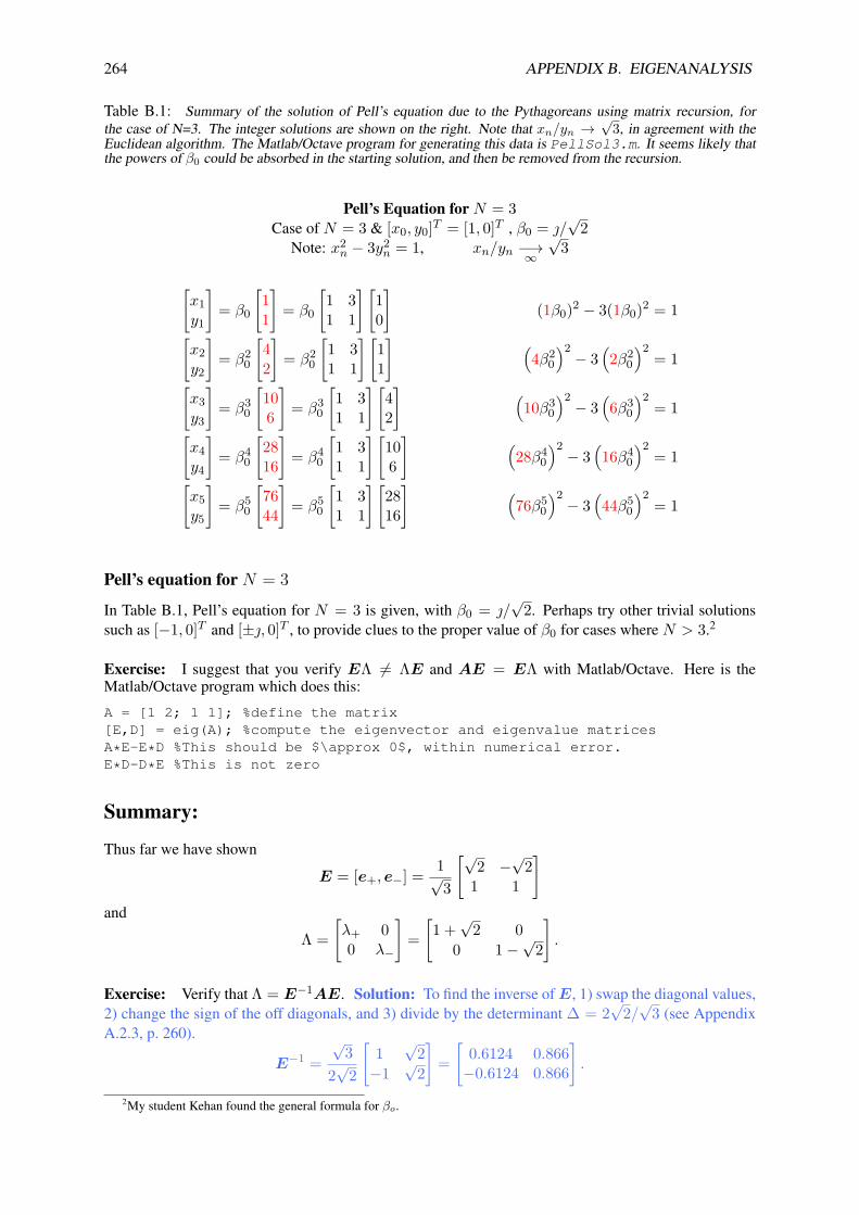
264 APPENDIX B. EIGENANALYSIS
Table B.1: Summary of the solution of Pell’s equation due to the Pythagoreans using matrix recursion, forthe case of N=3. The integer solutions are shown on the right. Note that xn/yn →
√3, in agreement with the
Euclidean algorithm. The Matlab/Octave program for generating this data is PellSol3.m. It seems likely thatthe powers of β0 could be absorbed in the starting solution, and then be removed from the recursion.
Pell’s Equation for N = 3Case of N = 3 & [x0, y0]T = [1, 0]T , β0 = /
√2
Note: x2n − 3y2
n = 1, xn/yn −→∞√
3
[x1y1
]= β0
[11
]= β0
[1 31 1
] [10
](1β0)2 − 3(1β0)2 = 1[
x2y2
]= β2
0
[42
]= β2
0
[1 31 1
] [11
] (4β2
0
)2− 3
(2β2
0
)2= 1[
x3y3
]= β3
0
[106
]= β3
0
[1 31 1
] [42
] (10β3
0
)2− 3
(6β3
0
)2= 1[
x4y4
]= β4
0
[2816
]= β4
0
[1 31 1
] [106
] (28β4
0
)2− 3
(16β4
0
)2= 1[
x5y5
]= β5
0
[7644
]= β5
0
[1 31 1
] [2816
] (76β5
0
)2− 3
(44β5
0
)2= 1
Pell’s equation for N = 3
In Table B.1, Pell’s equation for N = 3 is given, with β0 = /√
2. Perhaps try other trivial solutionssuch as [−1, 0]T and [±, 0]T , to provide clues to the proper value of β0 for cases where N > 3.2
Exercise: I suggest that you verify EΛ 6= ΛE and AE = EΛ with Matlab/Octave. Here is theMatlab/Octave program which does this:
A = [1 2; 1 1]; %define the matrix[E,D] = eig(A); %compute the eigenvector and eigenvalue matricesA*E-E*D %This should be $\approx 0$, within numerical error.E*D-D*E %This is not zero
Summary:
Thus far we have shown
E = [e+, e−] = 1√3
[√2 −
√2
1 1
]and
Λ =[λ+ 00 λ−
]=[1 +√
2 00 1−
√2
].
Exercise: Verify that Λ = E−1AE. Solution: To find the inverse ofE, 1) swap the diagonal values,2) change the sign of the off diagonals, and 3) divide by the determinant ∆ = 2
√2/√
3 (see AppendixA.2.3, p. 260).
E−1 =√
32√
2
[1√
2−1
√2
]=[
0.6124 0.866−0.6124 0.866
].
2My student Kehan found the general formula for βo.

B.3. SYMBOLIC ANALYSIS OF TE = EΛ 265
By definition for any matrix E−1E = EE−1 = I2. Taking the product gives
E−1E = √
32√
2
[1√
2−1
√2
]· 1√
3
[√2 −
√2
1 1
]=[1 00 1
]= I2.
We wish to show that Λ = E−1AE[1 +√
2 00 1−
√2
]. = √
32√
2
[1√
2−1
√2
]·[1 21 1
]· 1√
3
[√2 −
√2
1 1
],
which is best verified with Matlab.
Exercise: Verify thatA = EΛE−1. Solution: We wish to show that[1 21 1
]= 1√
3
[√2 −
√2
1 1
]·[1 +√
2 00 1−
√2
].√
32√
2
[1√
2−1
√2
].
All the above equations have been verified with Octave.
Eigenmatrix diagonalization is helpful in generating solutions for finding the solutions of Pell’s andFibonacci’s equations using transmission matrices.
Example: If the matrix corresponds to a transmission line, the eigenvalues have units of seconds [s][V +
V −
]n
=[e−sTo 0
0 esTo
] [V +
V −
]n+1
. (B.9)
In the time domain the forward traveling wave v+n+1(t − (n + 1)To) = v+
n (t − nTo) is delayed by To.Two applications of the matrix delays the signal by 2To (See discussion in §5.7.1, p. 217).
B.3 Symbolic analysis of TE = EΛ
B.3.1 The 2× 2 Transmission matrix:
Here we assume
T =[
A BC D
]with ∆T = 1.
The eigenvectors e± of T are
e± =(
12C
[(A −D )∓
√(A −D )2 + 4BC
]1
)(B.10)
and eigenvalues are
λ± = 12
((A + D )−
√(A −D )2 + 4BC
(A + D ) +√
(A −D )2 + 4BC
). (B.11)
The term under the radical (i.e., the discriminant) may be rewritten in terms of the determinant of T(i.e., ∆T = AD −BC ), since
(A −D )2 − (A + D )2 = −4AD .
The for the ABCD matrix the expression under the radical becomes
(A −D )2 + 4BC = A 2 + D 2 − 4AD + 4BC
= A 2 + D 2 − 4∆T .

266 APPENDIX B. EIGENANALYSIS
Rewriting the eigenvectors and eigenvalues in terms of ∆T we find
e± =(
12C
[(A −D )∓
√(A + D )2 − 4∆T
]1
)(B.12)
and
λ± = 12
((A + D )−
√(A + D )2 − 4∆T
(A + D ) +√
(A + D )2 − 4∆T
). (B.13)
B.3.2 Special cases having symmetry
For the case of the ABCD matrix the eigenvalues depend on reciprocity, since ∆T = 1 if T (s) isreciprocal, and ∆T = −1 if it is anti-reciprocal. Thus it is helpful to display the eigenfunctions andvalues in terms of ∆T so this distinction is explicit.
Reversible systems:
When A = D
E =[−√
BC +
√BC
1 1
]Λ =
[A −√
BC 00 A +
√BC
](B.14)
the transmission matrix is said to be reversible, and the properties greatly simplify.
Reciprocal systems
When the matrix is symmetric (B = C ), the corresponding system is said to be reciprocal. Most physicalsystems are reciprocal. The determinant of the transmission matrix of a reciprocal network ∆T =AD − BC = 1. For example, electrical networks composed of inductors, capacitors and resistors arealways reciprocal. It follows that the complex impedance matrix is symmetric (Van Valkenburg, 1964a).
Magnetic systems such as dynamic loudspeakers are anti-reciprocal, and correspondingly ∆T = −1.The impedance matrix of a loudspeaker is skew symmetric (Kim and Allen, 2013). All impedance matri-ces are either symmetric or anti-symmetric, depending on whether they are reciprocal (LRC networks)or anti-reciprocal (magnetic networks). These systems have complex eigenvalues with negative realparts, corresponding to lossy systems. In some sense, all of this follows from conservation of energy,but the precise general case is waiting for enlightenment. The impedance matrix is never Hermitian. Itis easily proved that Hermitian matrices have real eigenvalues, which correspond to lossless networks.Any physical system of equations that has any type of loss cannot be Hermitian.
In summary, given a reciprocal system, the T matrix has ∆T = 1, and the corresponding impedancematrix is symmetric (not Hermitian).
B.3.3 Impedance matrix
As previously discussed in §3.7 (p. 121), the T matrix corresponding to an impedance matrix is[V1V2
]= Z(s)
[I1I2
]= 1
C
[A ∆T
1 D
] [I1I2
].
Reciprocal systems have skew-symmetric impedance matrices, namely z12 = z21 (i.e., ∆T = 1). Whenthe system is both reversible A = D and reciprocal, the impedance matrix simplifies to
Z(s) = 1C
[A 11 A
].
For such systems there are only two degrees of freedom, A and C . As discussed previously in §3.7(p. 121), each of these has a physical meaning: 1/A is the Thevenin source voltage given a voltage driveand B/A is the Thevenin impedance (§3.9, p. 122).

B.3. SYMBOLIC ANALYSIS OF TE = EΛ 267
Impedance is not Hermitian: By definition, when a system is Hermitian its matrix is conjugate sym-metric
Z(s) = Z†(s),
a stronger condition than reciprocal, but not the symmetry of the Brune impedance matrix.

268 APPENDIX B. EIGENANALYSIS

Appendix C
Laplace Transforms
The definition of the LT may be found in §3.9.
C.1 Properties of the Laplace Transform
1. Time t ∈ R [s] and Laplace frequency [rad] are defined as s = σ + ω ∈ C.
2. Given a Laplace transform (LT ) pair f(t)↔ F (s), in the engineering literature, the time domainis always lower case [f(t)] and causal (i.e., f(t < 0) = 0) and the frequency domain is upper-case [e.g. F (s)]. Maxwell’s venerable equations are the unfortunate exception to this otherwiseuniversal rule.
3. The target time function f(t < 0) = 0 (i.e., it must be causal). The time limits are 0− < t < ∞.Thus the integral must start from slightly below t = 0 to integrate over a delta function at t = 0.For example if f(t) = δ(t), the integral must include both sides of the impulse. If you wish toinclude non-causal functions such as δ(t + 1), it is necessary to extend the lower time limit. Insuch cases simply set the lower limit of the integral to −∞, and let the integrand (f(t)) determinethe limits.
4. When taking the forward transform (t → s), the sign of the exponential is negative. This isnecessary to assure that the integral converges when the integrand f(t) → ∞ as t → ∞. Forexample, if f(t) = etu(t) (i.e., without the negative σ exponent), the integral does not converge.
5. The limits on the integrals of the reverse LTs are [σo−∞, σo+∞] ∈ C. These limits are furtherdiscussed in §4.7.2 (p. 181).
6. When taking the inverse Laplace transform, the normalization factor of 1/2π is required to cancelthe 2π in the differential ds of the integral.
7. The frequencies for the LT must be complex, and in general F (s) is complex analytic for σ > σo.It follows that the real and imaginary parts of F (s) are related by the CR conditions. Given<F (s) it is possible to find =F (s) (Boas, 1987). More on this in §4.2.2 (p. 149).
8. To take the inverse Laplace transform, we must learn how to integrate in the complex s plane.This will be explained in §4.5-4.7.2 (p. 167-181).
9. The Laplace step function is defined as
u(t) =∫ t
−∞δ(t)dt =
1 if t > 0NaN t = 00 if t < 0
.
Alternatively one could define δ(t) = du(t)/dt.
269

270 APPENDIX C. LAPLACE TRANSFORMS
10. It is easily shown that u(t)↔ 1/s by direct integration
F (s) =∫ ∞
0u(t) e−stdt = −e
−st
s
∣∣∣∣∣∞
o
= 1s.
With the LT step (u(t)) there is no Gibbs ringing effect.
11. The Laplace transform of a Brune impedance takes the form of a ratio of two polynomials. In suchcase the roots of the numerator polynomial are called the zeros while the roots of the denominatorpolynomial are called the poles. For example the LT of u(t) ↔ 1/s has a pole at s = 0, whichrepresents integration, since
u(t) ? f(t) =∫ r
−∞f(τ)dτ ↔ F (s)
s.
12. The LT is quite different from the FT in terms of its analytic properties. For example, the stepfunction u(t)↔ 1/s is complex analytic everywhere, except at s = 0. The FT of 1↔ 2πδ(ω) isnot analytic anywhere.
13. Dilated step function (a ∈ R)
u(at)↔∫ ∞−∞
u(at)e−stdt = 1a
∫ ∞−∞
u(τ)e−(s/a)τdτ = a
|a|1s
= ±1s,
where we have made the change of variables τ = at. The only effect that a has on u(at) is the signof t, since u(t) = u(2t). However u(−t) 6= u(t), since u(t) · u(−t) = 0, and u(t) + u(−t) = 1,except at t = 0, where it is not defined.
Once complex integration in the complex plane has been defined (§4.2.2, p. 149), we can justifythe definition of the inverse LT (Eq. 3.23).1
1https://en.wikipedia.org/wiki/Laplace_transform#Table_of_selected_Laplace_transforms

C.2. TABLES OF LAPLACE TRANSFORMS 271
C.2 Tables of Laplace transforms
Table C.1: Functional relationships between Laplace transforms.
LT functional properties
f(t) ? g(t) =∫ t
t=0f(t− τ)g(τ)dτ ↔ F (s)G(s) convolution
u(t) ? f(t) =∫ t
0−f(t)dt↔ F (s)
sconvolution
f(at)u(at)↔ 1aF (sa
) a ∈ R 6= 0 scaling
f(t)e−atu(t)↔ F (s+ a) damped
f(t− T )e−a(t−T )u(t− T )↔ e−sTF (s+ a) damped and delayed
f(−t)u(−t)↔ F (−s) reverse time
f(−t)e−atu(−t)↔ F (a− s) time-reversed & dampedd
dtf(t) = δ′(t) ? f(t)↔ sF (s) deriv
sin(t)u(t)t
↔ tan−1(1/s) half-sync
C.3 Symbolic transforms
Octave/Matlab allows one to find LT symbolic forms. Below are some examples that are known to workwith Octave version 4.2 and Matlab R2015a.
Table C.2: Symbolic relationships between Laplace transforms. K3 is a constant.
syms command result
syms t s p laplace(t(p−1)
)Γ(p)s−p
syms s ilaplace(gamma(s)) ee−t
syms s t a ilaplace(exp(-a*s)/s,s,t) Heaviside(t− a)syms Gamma s t taylor(Gamma,s,t) 1
s − γ + s(γ2
2 + π2
12
)+
s2(+1
6 polygamma (2, 1)− γπ2
12 −γ3
6
)+
s3K3 + · · ·

272 APPENDIX C. LAPLACE TRANSFORMS
Table C.3: Laplace transforms of f(t), δ(t), u(t), rect(t),To, p, e,∈ R and F (s), G(s),s, a ∈ C. Given a Laplacetransform (LT ) pair f(t) ↔ F (s), the frequency domain will always be upper-case [e.g. F (s)] and the time domain lowercase [f(t)] and causal (i.e., f(t < 0) = 0). An extended table of transforms is given in Table C.4 on page 273.
f(t)↔ F (s) t ∈ R; s, F (s) ∈ C Name
δ(t)↔ 1 Dirac
δ(|a|t)↔ 1|a|
a 6= 0 time-scaled Dirac
δ(t− To)↔ e−sTo delayed Dirac
δ(t− To) ? f(t)↔ F (s)e−sTo –∞∑n=0
δ(t− nTo) = 11− δ(t− To)
↔ 11− e−sTo =
∞∑n=0
e−snTo one-sided impulse train
u(t)↔ 1s
step
u(−t)↔ −1s
anti-causal step
u(at)↔ a
sa 6= 0 ∈ R dilated or reversed step
e−atu(t)↔ 1s+ a
a > 0 ∈ R damped step
cos(at)u(t)↔ 12
( 1s− a
+ 1s+ a
)a ∈ R cos
sin(at)u(t)↔ 12
( 1s− a
− 1s+ a
)a ∈ C “damped” sin
u(t− To)↔1se−sTo T0 > 0 ∈ R time delay
rect(t) = 1To
[u(t)− u(t− To)]↔1To
(1− e−sTo
)rect-pulse
u(t) ? u(t) = tu(t)↔ 1/s2 ramp
u(t) ? u(t) ? u(t) = 12 t
2u(t)↔ 1/s3 double ramp
1√tu(t)↔
√π
s
tpu(t)↔ Γ(p+ 1)sp+1 <p > −1, q ∈ C
Jn(ωot)u(t)↔
(√s2 + ω2
o − s)n
ωno√s2 + ω2
o

C.3. SYMBOLIC TRANSFORMS 273
Table C.4: The following table provides an extended table of Laplace Transforms. J0, K1 are Bessel functions of the firstand second kind.
f(t)↔ F (s) Name
δ(at)↔ 1a
a 6= 0; Time-scaled Dirac
δ(t+ To)↔ esTo negative delay
u(at)↔ a
sa 6= 0; dilate
u(−t)↔ −1s
anti-causal step
eatu(−t)↔ 1−s+ a
anticausal damped step
d1/2
dt1/2f(t)u(t)↔
√sF (s) “half” derivative
d1/2
dt1/2u(t)↔
√s “half” derivative
d
dt
1√πtu(t)↔ s√
s=√s semi-inductor
1√πtu(t)↔ 1√
s“half” integration
erfc(α√t)↔ 1
se−2α
√s (Morse-Feshbach-II, p. 1582) α > 0; erfc
Jo(at)u(t)↔ 1√s2 + a2
Bessel
J1(t)u(t)/t↔√s2 + 1− s
J1(t)u(t)/t+ 2u(t)↔√s2 + 1 + s = esinh−1(s)
δ(t) + J1(t)u(t)/t↔√s2 + 1
Io(t)u(t)↔ 1/√s2 − 1
u(t)/√t+ 1↔ es
√π
serfc(√s)
√tu(t) ∗
√1 + tu(t)↔ es/2K1(s/2)/2s

274 APPENDIX C. LAPLACE TRANSFORMS
C.3.1 LT −1 of the Riemann zeta function
Let z ≡ esT where T is the “sample period” at which data is taken (every T seconds). For example ifT = 22.7 = 1/44100 seconds then the data is sampled at 44100 k [Hz]. This is how a CD player workswith high quality music. Thus the unit-time delay operator z−1 as
δ(t− T )↔ e−sT
However when dealing with the Euler and Riemann zeta function, the only sampling rate that phys-ically makes sense, is T = 1 [s] (i.e. n ∈ I). In this case, the samples of interest are mod(n,πk).
The zeta function The zeta function depends explicitly on the primes, which makes it very important.In 1737 Euler proposed the real-valued function ζ(x) ∈ R and x ∈ R, to prove that the number ofprimes is infinite (Goldstein, 1973). Euler’s definition of ζ(x) ∈ R is given by the power series
ζ(x) =∞∑n=1
1nx
forx > 1 ∈ R. (C.1)
This series converges for x > 0, since R = n−x < 1, n > 1 ∈ N.2
In 1860 Riemann extended the zeta function into the complex plane, resulting in ζ(s), defined by thecomplex analytic power series, identical to the Euler formula, except x ∈ R has been replaced by s ∈ C
ζ(s) ≡ 11s + 1
2s + 13s + 1
4s + · · · =∞∑n=1
1ns
=∞∑n=1
n−s for<s = σ > 1. (C.2)
This formula converges for <s > 1 (Goldstein, 1973). To determine the formula in other regions ofthe s plane one must extend the series via analytic continuation. As it turns out, Euler’s formulationprovided detailed information about the structure of primes, going far beyond his original goal.
Euler product formula
As was first published by Euler in 1737, one may recursively factor out the leading prime term, resultingin Euler’s product formula. Euler’s procedure is an algebraic implementation of the sieve of Eratosthenes(§2.4, p. 40 and §5.1, page 187).
Multiplying ζ(s) by the factor 1/2s, and subtracting from ζ(s), removes all the even terms ∝1/(2n)s (e.g., 1/2s + 1/4s + 1/6s + 1/8s + · · · )(
1− 12s)ζ(s) = 1 + 1
2s + 13s + 1
4s + 15s · · · −
( 12s + 1
4s + 16s + 1
8s + 110s + · · ·
), (C.3)
which results in (1− 2−s
)ζ(s) = 1 + 1
3s + 15s + 1
7s + 19s + 1
11s + 113s + · · · . (C.4)
Repeating this with a lead factor 1/3s applied to Eq. C.4 gives3
13s(1− 2−s
)ζ(s) = 1
3s + 19s + 1
15s + 121s + 1
27s + 133s + · · · . (C.5)
Subtracting Eq. C.5 from Eq. C.4 cancels the RHS terms of Eq. C.4, giving(1− 3−s
) (1− 2−s
)ζ(s) = 1 + 1
5s + 17s + 1
11s + 113s + 1
17s + 119s · · · .
2Sanity check: For example let n = 2 and x > 0. Then R = 2−ε < 1, where ε ≡ lim x→ 0+. Taking the log giveslog2 R = −ε log2 2 = −ε < 0. Since logR < 0, R < 1.
3This is known as Euler’s sieve, as distinguish from the Eratosthenes sieve.
C.3. SYMBOLIC TRANSFORMS 275
Further repeating this process, with prime scale factors, (i.e., 1/5s, 1/7s, · · · , 1/πsk, · · · ), removes all theterms on the RHS but 1, which results in Euler’s analytic product formula (s = x ∈ R) and Riemann’scomplex analytic product formula (s ∈ C)
ζ(s) = 11− 2−s ·
11− 3−s ·
11− 5−s ·
11− 7−s · · ·
11− π−sn
· · ·
=∏k
11− πk−s
=∏πk∈P
ζk(s), (C.6)
where πk represents the kth prime and
ζk(s) = 11− π−sk
(C.7)
defines each prime factor. Each recursive step in this construction assures that the lead term, alongwith all of its multiplicative factors, are subtracted out, just as with the cancellations with the sieve ofEratosthenes. It is instructive to compare each iteration with that of the sieve (Fig. 2.2, p. 41).
The kth term of the complex analytic Riemann product formula may be re-expressed as
|π−sk | = |e−sTk | < 1,
where Tk = ln πk. This relation defines the RoC of ζk as σk < ln πk. It would seem that since 1/πk < 1for all k ∈ N, the taylor series of ζk(x) is entire except at its poles. Note that the RoC of a Taylor seriesin powers of π−sk increases with k.
Exercise: Work out the RoC for k = 2. Solution: Todo
Exercise: Show how to construct Zeta2(t) ↔ ζ2(s) by working in the time domain. The basic rulesof building a sieve is to sum the integers
S1 =∞∑n=1
n2n−1 = 1 · 20 + 2 · 21 + 3 · 22 · · · ,
while the sieve for the kth prime πk is
Sk =∞∑n=1
nπn−1k = 1 · π0
k + πk · 21 + πk · 22 · · · .
This sum may be written in terms of the convolution with the step function uk since
uk ? uk = nuk = 0 · u0 + 1 · u1 + · · · kuk + · · · .
Here uk = 1 =∑n−∞ δk for k ≥ 0 and zero for k < 0, and δ0 = 1, and 0 for k 6= 0.
Poles of ζk(s)
Riemann proposed that Euler’s zeta function ζ(s) ∈ C have a complex argument (first actually exploredby Chebyshev in 1850, (Bombieri, 2000)), extending ζ(s) into the complex plane, (s ∈ C), making it acomplex analytic function.
Given that ζ(s) is a complex analytic function, one might naturally wonder if ζ(s) has an inverseLaplace transform. There seems to be very little written on this topic (Hill, 2007). We shall explore thisquestion further here.

276 APPENDIX C. LAPLACE TRANSFORMS
w = 1./(1-exp(-s*pi))
σ
-2 -1 0 1 2jω
2
1
0
-1
-2
Figure C.1: Plot of w(s) = 11−e−sπ . Here w(s) has poles where esn ln 2 = 1, namely where ωn ln 2 = n2π, as seen in
the colorized–map (s = σ + ω is the Laplace frequency [rad]).
One may now identify the poles of ζk(s) (p ∈ N), which are required to determining the RoC. Forexample, the kth factor of Eq. C.6, expressed as an exponential, is
ζk(s) ≡1
1− π−sk= 1
1− e−sTk =∞∑k=0
e−skTk , (C.8)
where Tk ≡ ln πk. Thus ζp(s) has poles at −snTp = 2πn (when e−sTp = 1), thus
ωn = 2πnTk
,
with −∞ < n ∈ Z < ∞. These poles are the eigenmodes of the zeta function. A domain-colorizedplot of this function is provided in Fig. C.1. It is clear that the RoC of ζk is > 0. It would be helpful todetermine why ζ(s) as such a more restrictive RoC than each of its factors.
+
Zetap (t)δ(t)
Delay
α = 1Zetap (t− Tp)
Zetap (t) = αZeta
p (n− Tp) + δ(t)
Tp
Figure C.2: This feedback network is described by a time-domain difference equation with delay Tp = lnπk, has anall-pole transfer function, given by Eq. C.11. Physically this delay corresponds to a delay of Tp [s].
Inverse Laplace transform
The inverse Laplace transform of Eq. C.8 is an infinite series of delays of delay Tp (Table C.3, p. 272)4
Zetap (t) = δ(t))Tp ≡∞∑k=0
δ(t− kTp)↔1
1− e−sTp . (C.9)
4Here we use a shorthand double-parentheses notation f(t))T ≡∑∞
k=0 f(t− kT ) to define the one-sided infinite sum.

C.3. SYMBOLIC TRANSFORMS 277
Inverse transform of Product of factors
The time domain version of Eq. C.6 may be written as the convolution of all the Zetak (t) factors
Zeta(t) ≡ Zeta2 ? Zeta3 (t) ? Zeta5 (t) ? Zeta7 (t) · · · ? Zetap (t) · · · , (C.10)
where ? represents time convolution (Table C.1, p. 271).
Physical interpretation
Such functions may be generated in the time domain as shown in Fig. C.2, using a feedback delay of Tp[s] as described by the equation in the figure, with a unity feedback gain α = 1.
Zeta(t) = Zeta(t− Tp) + δ(t).
Taking the Laplace transform of the system equation we see that the transfer function between the statevariable q(t) and the input x(t) is given by Zetap (t). Taking the LT , we see that ζ(s) is an all-polefunction
ζp(s) = e−sTpζp(s) + 1(t), or ζp(s) = 11− e−sTp . (C.11)
Discussion: In terms of the physics, these transmission line equations are telling us that ζ(s) may bedecomposed into an infinite cascade of transmission lines (Eq. C.10), each having a unique delay givenby Tk = ln πk, πk ∈ P, the log of the primes. The input admittance of this cascade may be interpretedas an analytic continuation of ζ(s) which defines the eigenmodes of that cascaded impedance function.
Working in the time domain provides a key insight, as it allows us to determine the analytic contin-uation of the infinity of possible continuations, which are not obvious in the frequency domain. Trans-forming to the time domain is a form of analytic continuation of ζ(s), that depends on the assumptionthat Zeta(t) is one-sided in time (causal).
Additional relations: Some important relations provided by both Euler and Riemann (1859) areneeded when studying ζ(s).
With the goal of generalizing his result, Euler extended the definition with the functional equation
ζ(s) = 2sπs−1 sin(πs
2
)Γ(1− s) ζ(1− s). (C.12)
This seems closely related to Riemann’s time reversal symmetry properties (Bombieri, 2000)
π−s/2Γ(s
2
)ζ(s) = π−(1−s)/2Γ
(1− s2
)ζ(1− s).
This equation is of the form F(s2)ζ(s) = F
(1−s
2
)ζ(1− s) where F (s) = Γ(s)/πs.
As shown in Table C.1 the LT −1 of f(−t) ↔ F (−s) is simply a time-reversal. This leads to acausal and anti-causal function that are symmetric about <s = 1/2 (Riemann, 1859). It seems likelythis is an important insight into the Euler’s functional equation.
Riemann (1859, page 2) provides an alternate integral definition of ζ(s), based on the complexcontour integration5
2 sin(πs)Γ(s− 1)ζ(s) =
∮ ∞x=−∞
(−x)s−1
ex − 1 dx.−x→y=
∮ ∞y=−∞
(y)s−1
e−y − 1dx.
Given the ζk(s) it seems important to look at the inverse LT of ζk(1 − s), to gain insight into theanalytically extended ζ(s)
5Verify Riemann’s use of x, which is taken to be real rather than complex. This could be more natural (i.e., modern Laplacetransformation notation) if −x→ y→ z.

278 APPENDIX C. LAPLACE TRANSFORMS
Integral definition of the complex Gamma function Γ(s): The definition of the complex analyticGamma function (p. 271)
Γ(s+ 1) = sΓ(s) ≡∫ ∞
0ξseξdξ,
which is a generalization of the real integer factorial function n!.
ξ(t) =∫ ∞−∞
Γ(s+ 1)esξ ds2π
What is the RoC of ζ(s)? It is commonly stated that Euler’s and thus Riemann’s product formula isonly valid for <s > 1, however this does not seem to be actually proved (I could be missing this proof).Here I will argue that the product formula is entire except at the poles. Namely that the formula is valideverywhere other that at the poles.
The argument goes as follows: Starting from the product formula (Eq. C.6 (p. 275)), form the log-derivative and study the poles and residues:
D(s) ≡ d
dsln Πk
11− e−sTk
= −∞∑k=1
11− e−sTk
d
ds1− e−sTk
= −∑k
Tke−sTk
1− e−sTk ↔∞∑k=1
∞∑n=1
δ(t− nTk).
Here Tk = ln πk, as previously defined, and ↔ denotes the inverse Laplace transform, transformingD(s)↔ d(t), into the time domain. Note that d(t) is a causal function, composed of an infinite numberof delta functions (i.e., time delays), as outline by Fig. C.2 (p. 276).
Zeros of ζ(s) We are still left with the most important question of all “Where are the zeros of ζ(s)?”Equation C.11 has no zeros, it is an all-pole system. The cascade of many such systems is also all-pole.As I see it, the issue is what is the actual formula for ζ(s)?

Appendix D
Visco-thermal losses
D.1 Adiabatic approximation at low frequencies:
At very low frequencies the adiabatic approximation must break down. Above this frequency, viscousand thermal damping in air can become significant. In acoustics these two effects are typically ignored,by assuming that wave propagation is irrotational, thus is described by the scalar wave equation. How-ever this is an approximation.
As first explained by Kirchhoff (1868) and Helmholtz (1858), these two loss mechanisms are related;but to understand why is somewhat complicated, due to both the history and the mathematics. The fulltheory was first worked out by Kirchhoff (1868, 1974). Both forms of damping are due to two differentbut coupled diffusion effects, first from viscous effects, due to shear at the container walls, and secondfrom thermal effects, due to small deviations from adiabatic expansion (Kirchhoff, 1868, 1974). I believeultimately Einstein was eventually involved as a result of his studies on Brownian motion (Einstein,1905).1 2
Newton’s early development understandably ignored viscous and thermal losses, which can be sig-nificant in a thin region called the boundary layer, at acoustic frequencies when the radius of the con-tainer (i.e., the horn) becomes less than the viscous boundary layer (e.g., much less than 1 mm) asfirst described in Helmholtz (1858, 1863b, 1978). Helmholtz’s analysis (Helmholtz, 1863b) was soonextended to include thermal losses by Kirchhoff (1868, 1974, English translation), as succinctly sum-marized by Lord Rayleigh (1896), and then experimentally verified by Warren P. Mason (Mason, 1927,1928).
The mathematical nature of damping is that the propagation function κ(s) (i.e, complex wave num-ber) is extended to
κ(s) = s+ β0√s
c0, (D.1)
where the forwarded P− and backward P+ pressure waves propagate as
P±(s, x) = e−κ(s)x, e−κ(s)x (D.2)
with κ(s) the complex conjugate of κ(s), and <κ(s) > 0. The term β0√s effects both the real and
imaginary parts of κ(s). The real part is a frequency dependent loss and the imaginary part introduces afrequency dependent speed of sound (Mason, 1928).
D.1.1 Lossy wave-guide propagation
In the case of lossy wave propagation, the losses are due to viscous and thermal damping. The formu-lation of viscous loss in air transmission was first worked out by Helmholtz (1863a), and then extended
1See Ch. 3 of https://www.ks.uiuc.edu/Services/Class/PHYS498/.2https://en.wikipedia.org/wiki/Einstein_relation_(kinetic_theory)
279

280 APPENDIX D. VISCO-THERMAL LOSS
Figure D.1: This figure, taken from Mason (1928), compares the Helmholtz-Kirchhoff theory for |κ(f)| to Mason’s 1928experimental results measurement of the loss. The ratio of two powers (P1 and P2) are plotted (see Mason’s discussionimmediately below Fig. 4), and as indicated in the label: “10 log10 P1/P2 for 1 [cm] of tube length.” This is a plot of thetransmission power ratio in [dB/cm].
by Kirchhoff (1868), to include thermal damping (Rayleigh, 1896, Vol. II, p. 319). These losses areexplained by a modified complex propagation function κ(s) (Eq. D.1). Following his review of thesetheories, Crandall (1926, Appendix A) noted that the “Helmholtz-Kirchhoff” theory had never been ex-perimentally verified. Acting on this suggestion, Mason (1928) set out to experimentally verify theirtheory.
Mason’s specification of the propagation function
Mason’s results are reproduced here in Fig. D.1 as the solid lines for tubes of fixed radius between3.7–8.5 [mm], having a power reflectance given by
|ΓL(f)|2 =∣∣∣e−κ(f)L
∣∣∣2 [dB/cm]. (D.3)
The complex propagation function cited by Rayleigh (1896) is (Mason, 1928, Eq. 2)
κ(ω) = Pη′o√ω
2coS√
2ρo+ iω
co
1 + Pη′o
2S√
2ωρo
(D.4)
and the characteristic impedance is
zo(ω) =√P0γρo
[1 + Pγ′
2S√
2ωρo− Pγ′
2S√
2ωρo
], (D.5)
where S is the tube area and P is its perimeter. Mason specified physical constants for air to be ηo = 1.4(ratio of specific heats), ρo = 1.2 [kgm/m3] (density), co =
√P0ηo/ρo = 341.56 [m/s] (lossless
air velocity of sound at 23.5 [C]), P0 = 105 [Pa] (atmospheric pressure), µo = 18.6× 10⁻⁶ [Pa-s](viscosity). Based on these values, η′o is defined as the composite thermodynamic constant (Mason,1928)
η′0 = √µo[1 +
√5/2
(η1/2o − η−1/2
o
)]=√
18.6× 10⁻³[1 +
√5/2
(√1.4− 1/
√1.4)]
= 6.618× 10⁻³.

D.1. ADIABATIC APPROXIMATION AT LOW FREQUENCIES: 281
D.1.2 Impact of viscous and thermal losses
Assuming air at 23.5 [C], c0 =√η0P0/ρ0 ≈ 344 [m/s] is the speed of sound, η0 = cp/cv = 1.4 is
the ratio of specific heats, µ0 = 18.5 × 10⁻⁶ [Pa-s] is the viscosity, ρ0 ≈ 1.2 [kgm/m2] is the density,P0 = 105 [Pa] (1 atm).
Equation D.4 and the measured data are compared in Fig. D.1, reproduced from Mason’s Fig. 4,which shows that the wave speed drops from 344 [m/s] at 2.6 [kHz] to 339 [m/s] at 0.4 [kHz], a 1.5%reduction in the wave speed. At 1 [kHz] the loss is 1 [dB/m] for a 7.5 [mm] tube. Note that the loss andthe speed of sound vary inversely with the radius. As the radius approaches the boundary layer thickness,i.e., the radial distance such that the loss is e−1, the effect of the damping dominates the propagation.
With some significant algebra, Eq. D.4 may be greatly simplified to Eq. D.1.3 Numerically
βo = P
2Sη′o√ρo
= P
2S 6.0415× 10⁻³
For the case of a cylindrical waveguide the radius is R = 2S/P . Thus
βo = 1R
η′o√ρo
= 1R
6.0415× 10⁻³.
Here β0 = Pη′/2S√ρ0 is a thermodynamic constant, P is the perimeter of the tube and S the area(Mason, 1928).
For a cylindrical tube having radiusR = 2S/P , β0 = η′0/R√ρ. To get a feeling for the magnitude of
β0 consider a 7.5 [mm] tube (i.e., the average diameter of the adult ear canal). Then η′ = 6.6180×10⁻³
and β0 = 1.6110. Using these conditions the wave-number cutoff frequency is 1.6112/2π = 0.4131[Hz]. At 1 kHz the ratio of the loss over the propagation is β0/
√|s| = 1.6011/
√2π103 ≈ 2%. At 100
[Hz] this is a 6.4% effect.4
Cut-off frequency s0: The frequency where the loss-less part equals the lossy part is defined asκ(s0) = 0, namely
s0 + β0√s0 = 0.
Solving for s0 gives the real, and negative, pole frequency of the system
√s0 = −β0 = −6.0415× 10⁻³/R.
To get a feeling for the magnitude of β0 let R = 0.75/2 [cm] (i.e., the average radius of the adultear canal). Then
−√s0 = β0 = 6.0145×10⁻³/ 3.75×10⁻³ ≈ 1.6.
We conclude that the losses are insignificant in the audio range since for the case of the human ear canalf0 = β2
0/2π ≈ 0.407 [Hz].5
Note how the propagation function has a Helmholtz-Kirchhoff correction for both the real and imag-inary parts. This means that both the speed of sound and the damping are dependent on frequency,proportional to β0
√s/co. Note also that the smaller the radius, the greater the damping.
Summary: The Helmholtz-Kirchhoff theory of viscous and thermal losses results in a frequencydependent speed of sound, having a frequency dependence proportional to 1/
√ω (Mason, 1928, Eq. 4).
This corresponds to a 2% change in the sound velocity over the decade from 0.2-2 [kHz] (Mason, 1928,Fig. 5), in agreement with experiment.
3The real and imaginary parts of this expression, with s = iω, give Eq. D.1, 279.4/home/jba/Mimosa/2C-FindLengths.16/doc.2-c_calib.14/m/MasonKappa.m5/home/jba/Mimosa/2C-FindLengths.16/doc.2-c_calib.14/m/MasonKappa.m

282 APPENDIX D. VISCO-THERMAL LOSS

Appendix E
Number theory applications
E.1 Division with rounding method:
We would like to show that the GCD for m,n, k ∈ N (Eq. 2.4, p. 43) may be written in matrix as[mn
]k+1
=[0 11 −
⌊mn
⌋] [mn
]k
. (E.1)
This implements gcd(m,n) for m > n.This starts with k = 0,m0 = a, n0 = b. With this method there is no need to test if nn < mn, as
it is built into the procedure. The method uses the floor function bxc, which finds the integer part of x(bxc rounds toward −∞). Following each step we will see that the value nk+1 < mk+1. The methodterminates when nk+1 = 0 with gcd(a, b) = mk+1.
Below is 1-line vectorized code that is much more efficient than the direct matrix method of §E(p. 283):
function n=gcd2(a,b)
M=[abs(a);abs(b)]; %Save (a,b) in array M(2,1)
% done when M(1) = 0while M(1) ˜= 0disp(sprintf(’M(1)=%g, M(2)=%g ’,M(1),M(2)));M=[M(2)-M(1)*floor(M(2)/M(1)); M(1)]; %automatically sortedend %done
n=M(2); %GCD is M(2)
With a minor extension in the test for “end,” this code can be made to work with irrational inputs (e.g.,(nπ,mπ)).
This method calculates the number of times n < m must subtract from m using the floor function.This operation is the same as the mod function.1 Specifically
nk+1 = mk −⌊m
n
⌋nk (E.2)
so that the output is the definition of the remainder of modular arithmetic. This would have been obviousto anyone using an abacus, which explains why it was discovered so early.
Note that the next value ofm (M(1)) is always less than n (M(2)), and must remain greater or equalto zero. This one-line vector operation is then repeated until the remainder (M(1)) is 0. The gcd is then
1https://en.wikipedia.org/wiki/Modulo_operation
283

284 APPENDIX E. NUMBER THEORY APPLICATIONS
n (M(2)). When using irrational numbers, this still works except the error is never exactly zero, dueto IEEE 754 rounding. Thus the criterion must be that the error is within some small factor times thesmallest number (which in Matlab is the number eps = 2.220446049250313 ×10⁻¹⁶, as defined in theIEEE 754 standard.)
Thus without factoring the two numbers, Eq. E.2 recursively finds the gcd. Perhaps this is best seenwith some examples.
The GCD is an important and venerable method, useful in engineering and mathematics, but, as bestI know, is not typically taught in the traditional engineering curriculum.
GCD applied to polynomials: An interesting generalization is work with polynomials rather thannumbers, and apply the Euclidean algorithm.
The GCD may be generalized in several significant ways. For example what is the GCD of twopolynomials? To answer this question one must factor the two polynomials to identify common roots.
E.2 Derivation of the CFA matrix:
The CFA may be define starting from the basic definitions of the floor and remainder formulae. Startingfrom a decimal number x we split it into the decimal and remainder parts2 Starting with n = 0 andxo = x ∈ I, the integer part is
m0 = bxc ∈ N
and the remainder isr0 = x−m0.
Corresponding the the CFA, the next target x1 is for n = 1 is
x1 = r−10
and the integer part is m1 = bx1c. As in the case of n = 0, the integer part is
m1 = bx1c
and the remainder isr1 = x1 −m1.
The recursion for n = 2 is similar.To better appreciate what is happening it is helpful to write these recursion in a matrix format.
Rewriting the case of n = 1 and using the remainder formula for the ratio of two numbers p ≥ q ∈ Nwith q 6= 0. [
pq
]=[u1 11 0
] [r0r1
].
From the remainder formula, u1 = bp/qc.Continuing with n = 2 [
r0r1
]=[u2 11 0
] [r1r2
].
where u1 = br0/r1c.Continuing with n = 3 [
r1r2
]=[u3 11 0
] [r2r3
],
2The method presented here was developed by Yiming Zhang as a student project in 2019.

E.3. TAKING THE INVERSE TO GET THE GCD. 285
where u2 = br1/r2c.For arbitrary n we find [
rn−2rn−1
]=[un 11 0
] [rn−1rn
](E.3)
where un = brn−1/rnc.This terminates when rn = 0 in the above nth step when[
rn−2rn−1
]=[un 11 0
] [rn−1rn = 0
].
Example: Let p, q = 355, 113, which are coprime and set n = 1. Then Eq. E.3 becomes[355113
]=[3 11 0
] [ror1
]
since u1 = b355113c = 3. Solving for the RHS gives [ro; r1] = [113; 16] (355 = 113 · 3 + 16). To find
[r0; r1], take the inverse: [ror1
]=[0 11 −3
] [355113
].
For n = 2, with the right hand side from the previous step,[11316
]=[u2 11 0
] [r1r2
]
since u2 = b11316 c = 7. Solving for the RHS gives [r1; r2] = [16; 1] (113 = 16 · 7 + 1). It seems we are
done, but lets go one more step.For n = 3 we now have [
161
]=[u3 11 0
] [r1r2
]since u3 = b16
1 c = 16. Solving for the RHS gives [r1; r2] = [1; 0]. This confirms we are done sincer2 = 0.
Derivation of Eq. E.3: Equation Eq. E.3 is derived as follows. Starting from the target x ∈ R, define
p = bxc and q = 1x− p
∈ R.
These two relations for truncation and remainder allow us to write the general matrix recursion relationfor the CFA, Eq. E.3. Given p, q, continue with the above cfa method.
One slight problem with the above is that the output is on the right and the input on the left. Thuswe need to take the inverse of these relationships to turn this into a composition.
E.3 Taking the inverse to get the gcd.
Variables p, q are the remainders rn−1 and rn respectively. Using this notation with n− 1 gives Eq. E.3.Inverting this gives the formula for the GCD[
rn−1rn
]=[0 11 −
⌊rn−2rn−1
⌋] [rn−2rn−1
].
This terminates when rn = 0, and the gcd(p,q) is rn−1. Not surprisingly these equations mirrorEq 2.5 (p. 44), but with different indexing scheme and interpretation of the variables.
This then explains why Gauss called the CFA the Euclidean algorithm. He was not confused. Butsince they have an inverse relation, they are not strictly the same.

286 APPENDIX E. NUMBER THEORY APPLICATIONS
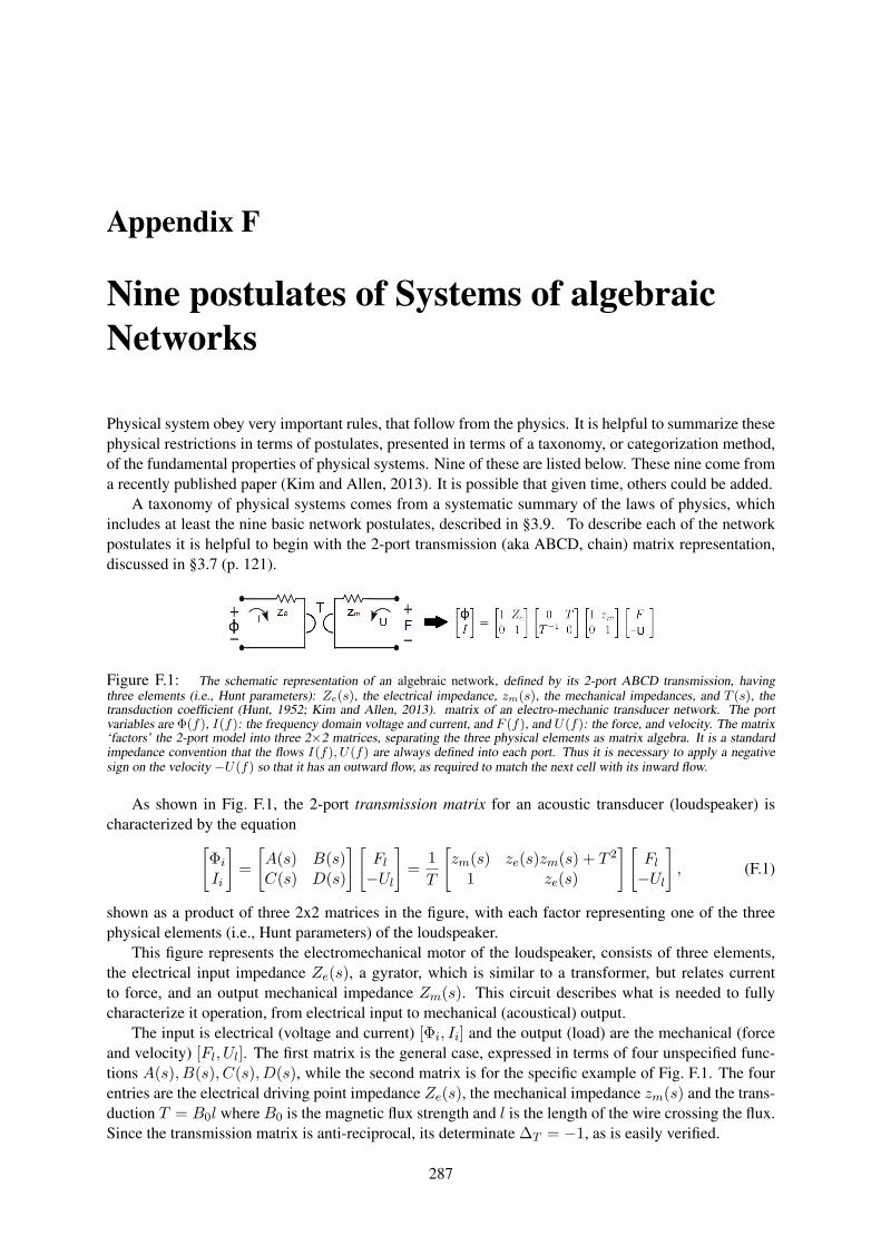
Appendix F
Nine postulates of Systems of algebraicNetworks
Physical system obey very important rules, that follow from the physics. It is helpful to summarize thesephysical restrictions in terms of postulates, presented in terms of a taxonomy, or categorization method,of the fundamental properties of physical systems. Nine of these are listed below. These nine come froma recently published paper (Kim and Allen, 2013). It is possible that given time, others could be added.
A taxonomy of physical systems comes from a systematic summary of the laws of physics, whichincludes at least the nine basic network postulates, described in §3.9. To describe each of the networkpostulates it is helpful to begin with the 2-port transmission (aka ABCD, chain) matrix representation,discussed in §3.7 (p. 121).
Figure F.1: The schematic representation of an algebraic network, defined by its 2-port ABCD transmission, havingthree elements (i.e., Hunt parameters): Ze(s), the electrical impedance, zm(s), the mechanical impedances, and T (s), thetransduction coefficient (Hunt, 1952; Kim and Allen, 2013). matrix of an electro-mechanic transducer network. The portvariables are Φ(f), I(f): the frequency domain voltage and current, and F (f), and U(f): the force, and velocity. The matrix‘factors’ the 2-port model into three 2×2 matrices, separating the three physical elements as matrix algebra. It is a standardimpedance convention that the flows I(f), U(f) are always defined into each port. Thus it is necessary to apply a negativesign on the velocity −U(f) so that it has an outward flow, as required to match the next cell with its inward flow.
As shown in Fig. F.1, the 2-port transmission matrix for an acoustic transducer (loudspeaker) ischaracterized by the equation[
Φi
Ii
]=[A(s) B(s)C(s) D(s)
] [Fl−Ul
]= 1T
[zm(s) ze(s)zm(s) + T 2
1 ze(s)
] [Fl−Ul
], (F.1)
shown as a product of three 2x2 matrices in the figure, with each factor representing one of the threephysical elements (i.e., Hunt parameters) of the loudspeaker.
This figure represents the electromechanical motor of the loudspeaker, consists of three elements,the electrical input impedance Ze(s), a gyrator, which is similar to a transformer, but relates currentto force, and an output mechanical impedance Zm(s). This circuit describes what is needed to fullycharacterize it operation, from electrical input to mechanical (acoustical) output.
The input is electrical (voltage and current) [Φi, Ii] and the output (load) are the mechanical (forceand velocity) [Fl, Ul]. The first matrix is the general case, expressed in terms of four unspecified func-tions A(s), B(s), C(s), D(s), while the second matrix is for the specific example of Fig. F.1. The fourentries are the electrical driving point impedance Ze(s), the mechanical impedance zm(s) and the trans-duction T = B0l where B0 is the magnetic flux strength and l is the length of the wire crossing the flux.Since the transmission matrix is anti-reciprocal, its determinate ∆T = −1, as is easily verified.
287

288 APPENDIX F. 9 SYSTEM POSTULATES
Other common transduction examples of cross-modality transduction include current–thermal (ther-moelectric effect) and force–voltage (piezoelectric effect). These systems are all reciprocal, thus thetransduction has the same sign.
Impedance matrix
These nine postulates describe the properties of a system having an input and an output. For the case ofan electromagnetic transducer (Loudspeaker) the system is described by the 2-port, as show in Fig. F.1.The electrical input impedance of a loudspeaker is Ze(s), defined by
Ze(s) = V (ω)I(ω)
∣∣∣∣U=0
.
Note that this driving-point impedance must be causal, thus it has a Laplace transform and therefore is afunction of the complex frequency s = σ+ jω, whereas the Fourier transforms of the voltage V (ω) andcurrent I(ω) are functions of the real radian frequency ω, since the time-domain voltage v(t) ↔ V (ω)and the current i(t)↔ I(ω) are signals that may start and stop at any time (they are not typically causal).
The corresponding 2-port impedance matrix for Fig. F.1 is[Φi
Fl
]=[z11(s) z12(s)z21(s) z22(s)
] [IiUl
]=[Ze(s) −T (s)T (s) zm(s)
] [IiUl
]. (F.2)
Such a description allows one to define Thevenin parameters, a very useful concept used widely incircuit analysis and other network models from other modalities.
The impedance matrix is an alternative description of the system, but with generalized forces [Φi, Fl]on the left and generalized flows [Ii, Ul] on the right. A rearrangement of the equations allows one togo from the ABCD to impedance set of parameters (Van Valkenburg, 1964b). The electromagnetictransducer is anti-reciprocal (P6), z12 = −z21 = T = B0l.
Taxonomy of algebraic networks
The postulates must go beyond postulates P1-P6 defined by Carlin and Giordano (§3.9, p. 131), whenthere are interaction of waves and a structured medium, along with other properties not covered byclassic network theory. Assuming QS, the wavelength must be large relative to the medium’s latticeconstants. Thus the QS property must be extended to three dimensions, and possibly to the cases ofan-isotropic and random media.
Causality: P1 As stated above, due to causality the negative properties (e.g., negative refractive index)must be limited in bandwidth, as a result of the Cauchy-Riemann conditions. However even causalityneeds to be extended to include the delay, as quantified by the d’Alembert solution to the wave equation,which means that the delay is proportional to the distance. Thus we generalize P1 to include the spacedependent delay. When we wish to discuss this property we denote it Einstein causality, which says thatthe delay must be proportional to the distance x, with impulse response δ(t− x/c).
Linearity: P2 The wave properties of may be non-linear. This is not restrictive as most physicalsystems are naturally nonlinear. For example, a capacitor is inherently nonlinear: as the charge buildsup on the plates of the capacitor, a stress is applied to the intermediate dielectric due to the electrostaticforce F = qE. In a similar manner, an inductor is nonlinear. Two wires carrying a current are attractedor repelled, due to the force created by the flux. The net force is the product of the two fluxes due toeach current.
In summary, most physical systems are naturally nonlinear, it’s simply a matter of degree. Animportant counter example is a amplifier with negative feedback, with very large open-loop gain. Thereare, therefore, many types of non-linear, instantaneous and those with memory (e.g., hysteresis). Given
289
the nature of P1, even an instantaneous non-linearity may be ruled out. The linear model is so criticalfor our analysis, providing fundamental understanding, that we frequently take P1 and P2 for granted.
Passive/Active: P3 This postulate is about conservation of energy and Otto Brune’s positive Real(PR aka physically realizable) condition, that every passive impedance must obey. Following up on theearlier work of his primary PhD thesis advisor Wilhelm Cauer (1900-1945) and Ernst Guillemin, alongwith Norbert Weiner and Vannevar Bush at MIT, Otto Brune mathematically characterized the propertiesof every PR 1-port driving point impedance (Brune, 1931b).
When the input resistance of the impedance is real, the system is said to be passive, which means thesystem obeys conservation of energy. The real part of Z(s) is positive if and only if the correspondingreflectance is less than 1 in magnitude. The definition of the reflectance of Z(s) is defined as a bilineartransformation of the impedance, normalized by its surge resistance r0 (Campbell, 1903a)
Γ(s) = Z(s)− r0Z(s) + r0
= Z − 1Z + 1
where Z = Z/ro. The surge resistance is defined in terms of the inverse Laplace transform of Z(s) ↔z(t), which must have the form
z(t) = r0δ(t) + ρ(t),
where ρ(t) = 0 for t < 0. It naturally follows that γ(t) ↔ Γ(s) is zero for negative and zero time,namely γ(0) = 0, t ≤ 0. at
Given any linear PR impedanceZ(s) = R(σ, ω)+jX(σ, ω), having real partR(σ, ω) and imaginarypart X(σ, ω), the impedance is defined as being PR (Brune, 1931b) if and only if
<Z(s) = R(σ ≥ 0, ω) ≥ 0. (F.3)
That is, the real part of any PR impedance is non-negative everywhere in the right half-plane (σ ≥ 0).This is a very strong condition on the complex analytic function Z(s) of a complex variable s. Thiscondition is equivalent to any of the following statements (Van Valkenburg, 1964a):
1. There are no poles or zeros in the right half-plane (Z(s) may have poles and zeros on the σ = 0axis).
2. If Z(s) is PR then its reciprocal Y (s) = 1/Z(s) is PR (the poles and zeros swap).
3. If the impedance may be written as the ratio of two polynomials (a limited case, related to thequasi-statics approximation, P9) having degrees N and L, then |N − L| ≤ 1.
4. The angle of the impedance θ ≡ ∠Z lies between [−π ≤ θ ≤ π].
5. The impedance and its reciprocal are complex analytic in the right half-plane, thus they each obeythe Cauchy Riemann conditions there.
Energy and Power: The PR (positive real or Physically realizable) condition assures that every im-pedance is positive-definite (PD), thus guaranteeing conservation of energy is obeyed (Schwinger andSaxon, 1968, p.17). This means that the total energy absorbed by any PR impedance must remainpositive for all time, namely
E (t) =∫ t
−∞v(t)i(t) dt =
∫ t
−∞i(t)?z(t) i(t) dt > 0,
where i(t) is any current, v(t) = z(t) ? i(t) is the corresponding voltage and z(t) is the real causalimpulse response of the impedance, e.g., z(t) ↔ Z(s) are a Laplace Transform pair. In summary, ifZ(s) is PR, E (t) is PD.

290 APPENDIX F. 9 SYSTEM POSTULATES
As discussed in detail by Van Valkenburg, any rational PR impedance can be represented as a partialfraction expansion, which can be expanded into first-order poles as
Z(s) = KΠLi=1(s− ni)
ΠNk=1(s− dk)
=∑n
ρns− sn
ej(θn−θd), (F.4)
where ρn is a complex scale factor (residue). Every pole in a PR function has only simple poles andzeros, requiring that |L−N | ≤ 1 (Van Valkenburg, 1964b).
Whereas the PD property clearly follows P3 (conservation of energy), the physics is not so clear.Specifically what is the physical meaning of the specific constraints on Z(s)? In many ways, the imped-ance concept is highly artificial, as expressed by P1-P7.
When the impedance is not rational, special care must be taken. An example of this is the semi-inductor M
√s and semi-capacitor K/
√s due, for example, to the skin effect in EM theory and viscous
and thermal losses in acoustics, both of which are frequency dependent boundary-layer diffusion losses(Vanderkooy, 1989). They remain positive-real but have a branch cut, thus are double valued in fre-quency.
Real time response: P4 The impulse response of every physical system is real, vs. complex. Thisrequires that the Laplace Transform have conjugate-symmetric symmetry H(s) = H∗(s∗), where the ∗indicates conjugation (e.g., R(σ, ω) +X(σ, ω) = R(σ, ω)−X(σ,−ω)).
Time invariant: P5 The meaning of time-invariant requires that the impulse response of a system doesnot change over time. This requires that the system coefficients of the differential equation describingthe system are constant (independent of time).
Rayleigh Reciprocity: P6 Reciprocity is defined in terms of the unloaded output voltage that resultsfrom an input current. Specifically (same as Eq. 3.12, p. 122) )[
z11(s) z12(s)z21(s) z22(s)
]= 1C(s)
[A(s) ∆T
1 D(s)
], (F.5)
where ∆T = A(s)D(s) − B(s)C(s) = ±1 for the reciprocal and anti-reciprocal systems respectively.This is best understood in term of Eq. F.2. The off-diagonal coefficients z12(s) and z21(s) are defined as
z12(s) = Φi
Ul
∣∣∣∣Ii=0
z21(s) = FlIi
∣∣∣∣Ul=0
.
When these off-diagonal elements are equal [z12(s) = z21(s)] the system is said to obey Rayleighreciprocity. If they are opposite in sign [z12(s) = −z21(s)], the system is said to be anti-reciprocal.If a network has neither of the reciprocal or anti-reciprocal characteristics, then we denote it as non-reciprocal (McMillan, 1946). The most comprehensive discussion of reciprocity, even to this day, is thatof Rayleigh (1896, Vol. I). The reciprocal case may be modeled as an ideal transformer (Van Valkenburg,1964a) while for the anti-reciprocal case the generalized force and flow are swapped across the 2-port.An electromagnetic transducer (e.g., a moving coil loudspeaker or electrical motor) is anti-reciprocal(Kim and Allen, 2013; Beranek and Mellow, 2012), requiring a gyrator rather than a transformer, asshown in Fig. F.1.
Reversibility: P7 A second 2-port property is the reversible/non-reversible postulate. A reversiblesystem is invariant to the input and output impedances being swapped. This property is defined by theinput and output impedances being equal.
Referring to Eq. F.5, when the system is reversible z11(s) = z22(s) or in terms of the transmissionmatrix variables A(s)
C(s) = D(s)C(s) or simply A(s) = D(s) assuming C(s) 6= 0.

291
An example of a non-reversible system is a transformer where the turns ratio is not one. Also anideal operational amplifier (when the power is turned on) is non-reversible due to the large impedancedifference between the input and output. Furthermore it is active (it has a power gain, due to the currentgain at constant voltage) (Van Valkenburg, 1964b).
Generalizations of this lead to group theory, and Noether’s theorem. These generalizations applyto systems with many modes whereas quasi-statics holds when operate below a cutoff frequency (TableF.1), meaning that like the case of the transmission line, there are no propagating transverse modes.While this assumption is never exact, it leads to highly accurate results because the non-propagatingevanescent transverse modes are attenuated over a short distance, and thus, in practice, may be ignored(Montgomery et al., 1948; Schwinger and Saxon, 1968, Chap. 9-11).
We extend the Carlin and Giordano postulate set to include (P7) Reversibility, which was refined byVan Valkenburg (1964a). To satisfy the reversibility condition, the diagonal components in a system’simpedance matrix must be equal. In other words, the input force and the flow are proportional to theoutput force and flow, respectively (i.e., Ze = zm).
Spatial invariant: P8 The characteristic impedance and wave number κ(s, x) may be strongly fre-quency and/or spatially dependent, or even be negative over some limited frequency ranges. Due tocausality, the concept of a negative group velocity must be restricted to a limited bandwidth (Brillouin,1960). As is made clear by Einstein’s theory of relativity, all materials must be strictly causal (P1), aview that must therefore apply to acoustics, but at a very different time scale. We first discuss generalizedpostulates, expanding on those of Carlin and Giordano.
The QS constraint: P9 When a system is described by the wave equation, delay is introduced betweentwo points in space, which depends on the wave speed. When the wavelength is large compared tothe delay, one may successfully apply the quasi-static approximation. This method has wide-spreadapplication, and is frequency used without mention of the assumption. This can lead to confusion,since the limitations of the approximation may not be appreciated. An example is the use of QS inQuantum Mechanics. The QS approximation has wide spread use when the signals may be accuratelyapproximated by a band-limited signal. Examples include KCL, KVL, wave guides, transmission lines,and most importantly, impedance. The QS property is not mentioned in the six postulates of Carlin andGiordano (1964), thus they need to be extended in some fundamental ways.
When the dimensions of a cellular structure in the material are much less than the wavelength, canthe QS approximation be valid. This effect can be viewed as a mode filter that suppresses unwanted (orconversely enhances the desired) modes (Ramo et al., 1965). QSs may be applied to a 3 dimensionalspecification, as in a semiconductor lattice. But such applications fall outside the scope of this text(Schwinger and Saxon, 1968).
Although I have never seen the point discussed in the literature, the QS approximation is appliedwhen defining Green’s theorem. For example, Gauss’s Law is not true when the volume of the containerviolates QS, since changes in the distribution of the charge have not reached the boundary, when doingthe integral. Thus such integral relationships assume that the system is in quasi steady-state (i.e., thatQS holds).
Formally, QS is defined as ka < 1 where k = 2π/λ = ω/c and a is the cellular dimension or thesize of the object. Other ways of expressing this include λ/4 > a, λ/2π > a, λ > 4a or λ > 2πa. It isnot clear if it is better to normalize λ by 4 (quarter-wavelength constraint) or 2π ≈ 6.28 > 4, which ismore conservative by a factor of π/2 ≈ 1.6. Also k and a can be vectors, e.g., Eq. 3.5 (p. 71).
Schelkunoff may have been the first to formalize this concept (Schelkunoff, 1943) (but not the firstto use it, as exemplified by the Helmholtz resonator). George Ashley Campbell was the first to usethe concept in the important application of a wave-filter, some 30 years before Schelkunoff (Campbell,1903a). These two men were 40 years apart, and both worked for the telephone company (after 1929,called AT&T Bell Labs) (Fagen, 1975).

292 APPENDIX F. 9 SYSTEM POSTULATES
Table F.1: There are several ways of indicating the quasi-static (QS) approximation. For network theory there is onlyone lattice constant a, which must be much less than the wavelength (wavelength constraint). These three constraints are notequivalent when the object may be a larger structured medium, spanning many wavelengths, but with a cell structure size muchless than the wavelength. For example, each cell could be a Helmholtz resonator, or an electromagnetic transducer (i.e., anearphone).
Measure Domainka < 1 Wavenumber constraintλ > 2πa Wavelength constraintfc < c/2πa Bandwidth constraint
There are alternative definitions of the QS approximation, depending on the geometrical cell struc-ture. The alternatives are outlined in Table F.1.
The quasi-static approximation: Since the velocity perpendicular to the walls of the horn must bezero, any radial wave propagation is exponentially attenuated (κ(s) is real and negative, i.e., the prop-agation function κ(s) (§4.4, p. 156) will not describe radial wave propagation), with a space constantof about 1 diameter. The assumption that these radial waves can be ignored (i.e., more than 1 diam-eter from their source) is called the quasi-static approximation. As the frequency is increased, oncef ≥ fc = 2co/λ, the radial wave can satisfy the zero normal velocity wall boundary condition, andtherefore will not be attenuated. Thus above this critical frequency, radial waves (aka, higher ordermodes) are supported (κ becomes imaginary). Thus for Eq. 5.29 to describe guided wave propagation,f < fc. But even under this condition, the solution will not be precise within a diameter (or so) of anydiscontinuities (i.e., rapid variations) in the area.
Each horn, as determined by the area function A(r), has a distinct wave equation, and thus a distinctsolution. Note that the area function determines the upper cutoff frequency via the quasi-static approx-imation since fc = c0/λc, λc/2 > d, A(r) = π(d/2)2. Thus to satisfy the quasi-static approximation,the frequency f must be less than the cutoff frequency
f < fc(r) = co4
√π
A(r) . (F.6)
We shall discuss two alternative matrix formulations of these equations: the ABCD transmissionmatrix, used for computation, and the impedance matrix, used when working with experimental mea-surements (Pierce, 1981, Chapter 7). For each formulation reciprocity and reversibility show up asdifferent matrix symmetries, as addressed in §3.9 (p. 131) (Pierce, 1981, p. 195-203).
Summary
A transducer converts between modalities. We propose the general definition of the nine system pos-tulates, that include all transduction modalities, such as electrical, mechanical, and acoustical. It isnecessary to generalize the concept of the QS approximation (P9) to allow for guided waves.
Given the combination of the important QS approximation, along with these space-time, linearity,and reciprocity properties, a rigorous definition and characterization a system can thus be established. Itis based on a taxonomy of such materials, formulated in terms of material and physical properties andin terms of extended network postulates.

Appendix G
Webster horn equation Derivation
In this section we transform the acoustic equations Eq. 5.24 and 5.25 (p. 202) into their equivalentintegral form Eq. 5.29 (p. 204). This derivation is similar (but not identical) to that of Hanna and Slepian(1924) and Pierce (1981, p. 360).
Conservation of momentum: The first step is an integration of the normal component of Eq. 5.24(p. 202) over the iso-pressure surface S , defined by∇p = 0
−∫
S∇p(x, t) · dA = ρo
∂
∂t
∫S
u(x, t) · dA.
The average pressure %(x, t) is defined by dividing by the total area
%(x, t) ≡ 1A(x)
∫Sp(x, t) n · dA. (G.1)
From the definition of the gradient operator
∇p = ∂p
∂xn, (G.2)
where n is a unit vector perpendicular to the iso-pressure surface S . Thus the left side of Eq. 5.24reduces to ∂%(x, t)/∂x.
The integral on the right side defines the volume velocity
ν(x, t) ≡∫S
u(x, t) · dA. (G.3)
Thus the integral form of Eq. 5.24 (p. 202) becomes
− ∂
∂x%(x, t) = ρo
A(x)∂
∂tν(x, t)↔ Z (x, s)V , (G.4)
whereZ (s, x) = sρo/A(x) = sM(x), (G.5)
and where M(x) = ρo/A(x) [kgm/m5] is the per-unit-length mass density of air.
Conservation of mass: Integrating Eq. 5.25 (p. 202) over the volume V gives
−∫V∇ · u dV = 1
ηoPo
∂
∂t
∫Vp(x, t)dV.
The volume V is defined by two iso-pressure surfaces between x and x+ δx (green region of Fig. G.1).On the right-hand side we use the definition of the average pressure (i.e., Eq. G.1), integrated over thevolume dV .
293
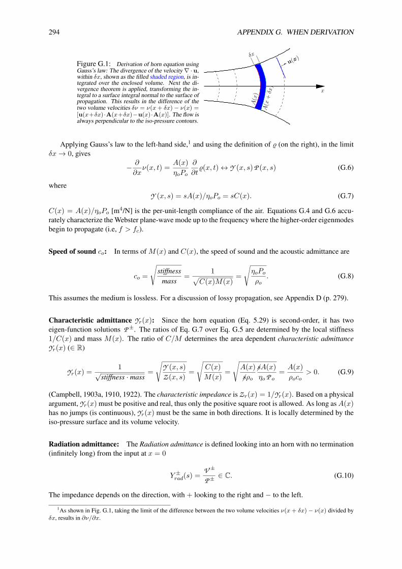
294 APPENDIX G. WHEN DERIVATION
Figure G.1: Derivation of horn equation usingGauss’s law: The divergence of the velocity∇ ·u,within δx, shown as the filled shaded region, is in-tegrated over the enclosed volume. Next the di-vergence theorem is applied, transforming the in-tegral to a surface integral normal to the surface ofpropagation. This results in the difference of thetwo volume velocities δν = ν(x+ δx)− ν(x) =[u(x+δx) ·A(x+δx)−u(x) ·A(x)]. The flow isalways perpendicular to the iso-pressure contours.
δx
x
A(x
)A
(x+δx
)
u(x)
Applying Gauss’s law to the left-hand side,1 and using the definition of % (on the right), in the limitδx→ 0, gives
− ∂
∂xν(x, t) = A(x)
ηoPo
∂
∂t%(x, t)↔ Y (x, s) P (x, s) (G.6)
whereY (x, s) = sA(x)/ηoPo = sC(x). (G.7)
C(x) = A(x)/ηoPo [m4/N] is the per-unit-length compliance of the air. Equations G.4 and G.6 accu-rately characterize the Webster plane-wave mode up to the frequency where the higher-order eigenmodesbegin to propagate (i.e, f > fc).
Speed of sound co: In terms of M(x) and C(x), the speed of sound and the acoustic admittance are
co =
√stiffness
mass= 1√
C(x)M(x)=√ηoPoρo
. (G.8)
This assumes the medium is lossless. For a discussion of lossy propagation, see Appendix D (p. 279).
Characteristic admittance Yr(x): Since the horn equation (Eq. 5.29) is second-order, it has twoeigen-function solutions P ±. The ratios of Eq. G.7 over Eq. G.5 are determined by the local stiffness1/C(x) and mass M(x). The ratio of C/M determines the area dependent characteristic admittanceYr(x) (∈ R)
Yr(x) = 1√stiffness · mass
=√
Y (x, s)Z (x, s) =
√C(x)M(x) =
√A(x)sρo
sA(x)ηo P o
= A(x)ρoco
> 0. (G.9)
(Campbell, 1903a, 1910, 1922). The characteristic impedance is Zr(x) = 1/Yr(x). Based on a physicalargument, Yr(x) must be positive and real, thus only the positive square root is allowed. As long asA(x)has no jumps (is continuous), Yr(x) must be the same in both directions. It is locally determined by theiso-pressure surface and its volume velocity.
Radiation admittance: The Radiation admittance is defined looking into an horn with no termination(infinitely long) from the input at x = 0
Y ±rad(s) = V ±
P ±∈ C. (G.10)
The impedance depends on the direction, with + looking to the right and − to the left.
1As shown in Fig. G.1, taking the limit of the difference between the two volume velocities ν(x+ δx)− ν(x) divided byδx, results in ∂ν/∂x.

295
The input admittance Y ±in (x, s) is computed using the upper equation of Eq. 5.30 (p. 205) forV (x, s), and then divide by the pressure eigen function P ±. This results in the logarithmic deriva-tive of P ±(x, s)
Y ±in (x, s) ≡ V ±
P ±= −1sM(x)
∂
∂rln P ±(x, s).
For example, for the conical horn, (last column of Table 5.2)
Y ±in = Yr(1± co/sro). (G.11)
Note that Y +in (x, s) + Y −in (x, s) = 2Yr = 2A0r
2/ρoco ∈ R, which shows that the frequency dependentpart of the two admittances, begin equal and opposite in sign, exactly cancel.
As the wavefront travels down the variable area horn, there is a mismatch in the characteristic ad-mittance due to the change in area. This mismatch creates a reflected wave, which in the case of theconical horn is = −co/sro. Due to conservation of volume, there is a corresponding identical forwardcomponent that travels forward, equal to +co/sro. The sum of these two responses, due to the changein area, must be zero, to conserve volume velocity.
The resulting equation for the velocity eigen-functions is therefore
V ±(x, s) = Y ±in (x.s) P ±(x, s).
Propagation function κ(s) The eigen-functions of the lossless wave equation propagate as
P ±(x, s) = e∓κ(s)x√A(x)
where κ(s) =√
Z (x, s)Y (x, s) = ±s√MC. The velocity eigen-functions V ±(x, s) may be computed
from Eq. G.4.From the above definitions
κ(s) =√
sρo
A(x)sA(x)
ηoPo= s
co.
Thus κ(s) and s are the eigenvalues of the differential operations ∂/∂x and ∂/∂t operating on thepressure P (x, s). See appendix D for the inclusion of visco-thermal losses.

296 APPENDIX G. WHEN DERIVATION

Appendix H
MATHEMATICSENGINEERING
PHYSICS
Figure H.1: Venn diagram showning relations between Engineering, Mathematics and Physics (p. 9).
Figure H.2: Fibonacci spiral (p. 60).
ℜ x
0 1 2 3 4 5
ℑ x
-2
-1
0
1
2
ℜ x
0 1 2 3 4 5
ℑ x
-2
-1
0
1
2
Figure H.3: Newtons method, applied to two polynomials: real roots (left); complex roots (right) (p. 75).
297

298 APPENDIX H. COLOR PLATES
w = s
σ
-2 -1 0 1 2
jω
2
1
0
-1
-2
w = s-sqrt(j)
σ
-2 -1 0 1 2
jω
2
1
0
-1
-2
Figure H.4: Colorized plots: Left: trivial case w(s) = s; Right: w(s) = s− (p. 135).
w = sin(0.5*pi*(s-j))
σ
-2 -1 0 1 2
jω
2
1
0
-1
-2
Figure H.5: w(s) = sin(0.5π(s− i)) (p. 136).
w = exp(s)
σ
-2 -1 0 1 2
jω
2
1
0
-1
-2
s = log(z)
x-2 -1 0 1 2
jy
2
1
0
-1
-2
Figure H.6: Colorized plots of w(z) = ez (left) and w(z) = ln(z) (right) (p. 137).

299
s = atan(z)
x-2 -1 0 1 2
jy
2
1
0
-1
-2
s = (i/2)*log((1-i*z)./(1+i*z))
x-2 -1 0 1 2
jy
2
1
0
-1
-2
Figure H.7: Plots of w(z) = atan(z) (left) and w(z) = ı2 ln 1−ız
1+ız (right) (p. 147).
w = s.^2
σ
-2 -1 0 1 2
jω
2
1
0
-1
-2
w = -sqrt(-s)
σ
-2 -1 0 1 2
jω
2
1
0
-1
-2
Figure H.8: Colorized plots of w(s) = s2 (left) and w(s) = −√s (right) (p. 163).
Figure H.9: Plot of 3D version of w(s) = ±√s showing both ±sheets and cut on x = 0 (p. 161).

300 APPENDIX H. COLOR PLATES
w = s
σ
-2 -1 0 1 2
jω
2
1
0
-1
-2
w = sqrt(s)
σ
-2 -1 0 1 2
jω
2
1
0
-1
-2
w = exp(j*pi).*sqrt(s)
σ
-2 -1 0 1 2
jω
2
1
0
-1
-2
Figure H.10: Plots of w(s) = s, w(s) =√s and w(s) = eπ
√s (p. 164).
w = sqrt(pi./s)
σ
-2 -1 0 1 2
jω
2
1
0
-1
-2
w = sqrt(s.^2+1)
σ
-2 -1 0 1 2
jω
2
1
0
-1
-2
Figure H.11: Plot of w(s) =√π/s (left) and w(s) =
√s2 + 1 (right) (p. 165).

301
s = cos(pi*z)
x-2 -1 0 1 2
jy 2
1
0
-1
-2
s = besselj(0,pi*z)
x-2 -1 0 1 2
jy
2
1
0
-1
-2
Figure H.12: Plot of w(s) = cos(πz) (right) and w(z) = J0(πz) (left) (p. 179).
s = besselj(0,pi*z)
x-2 -1 0 1 2
jy
2
1
0
-1
-2
s = besselh(0,1,pi*z/2)
x-2 -1 0 1 2
jy
2
1
0
-1
-2
Figure H.13: Plot of Bessel function J0(πz) and Hankel function H(1)0 (πz/2) (p. 180).
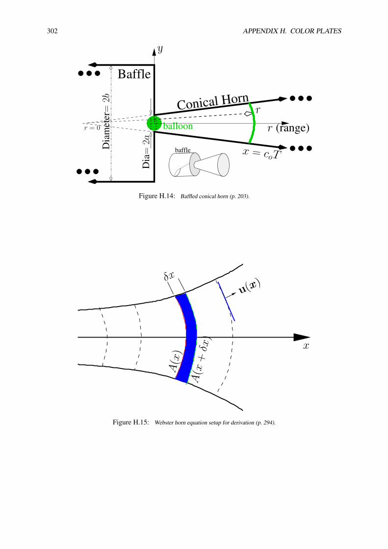
302 APPENDIX H. COLOR PLATES
baffle
Baffle
balloon
Conical Horn
Dia
=2aDia
met
er=
2b
r = 0
r
y
r (range)
x = coT
Figure H.14: Baffled conical horn (p. 203).
δx
x
A(x
)A
(x+δx
)
u(x)
Figure H.15: Webster horn equation setup for derivation (p. 294).

Bibliography
Allen, J. B. (2014), “The relation between tympanic membrane higher order modes and standing waves.”in Proceedings of the 12th International Mechanics of Hearing Workshop, Greece, edited by D. Coreyand K. Karavitaki (AIP, American Institute of Physics, Melville, NY), pp. 1–8.
Apel, W. (2003), The Harvard dictionary of music (Harvard University Press).
Apte, S. (2009), “The genius germs hypothesis: Were epidemics of leprosy and tuberculosis responsiblein part for the great divergence,” Hypothesis 7(1), e3,http://www.hypothesisjournal.com/wp-content/uploads/2011/09/vol7no1-hj003.pdf,
https://en.wikipedia.org/wiki/Joseph_Needham.
Arnold, Douglas and Rogness, Jonathan (2019), “Mobius Transformations Revealed,” Youtube.com,Video explaining the Riemann sphere:https://www.youtube.com/watch?v=0z1fIsUNhO4.
Batchelor, G. (1967), An introduction to fluid dynamics (Cambridge University Press, Cambridge,United Kingdom).
Beranek, L. L. (1954), Acoustics (McGraw–Hill Book Company, Inc., 451 pages, New York).
Beranek, L. L. and Mellow, T. J. (2012), Acoustics: Sound Fields and Transducers (Academic Press -Elsevier Inc., Waltham, MA).
Boas, R. (1987), An invitation to Complex Analysis (Random House, Birkhauser Mathematics Series).
Bode, H. (1945), Network Analysis and Feedback Amplifier Design (Van Nostrand, New York).
Bombieri, E. (2000), “Problems of the millennium: The Riemann hypothesis,” RiemannZeta-ClayDesc.pdf , 1–11Date unknown.
Boyer, C. and Merzbach, U. (2011), A History of Mathematics (Wiley),https://books.google.com/books?id=BokVHiuIk9UC .
Brillouin, L. (1953), Wave propagation in periodic structures (Dover, London), updated 1946 editionwith corrections and added appendix.
Brillouin, L. (1960), Wave propagation and group velocity (Academic Press), pure and Applied Physics,v. 8, 154 pages.
Britannica, E. (2004), Encyclopædia Britannica Online (Britannica Online),https://en.wikipedia.org/wiki/Pierre-Simon_Laplace.
Brune, O. (1931a), “Synthesis of a finite two-terminal network whose driving point impedance is aprescribed function of frequency,” J. Math and Phys. 10, 191–236.
Brune, O. (1931b), “Synthesis of a finite two-terminal network whose driving point impedance is aprescribed function of frequency,” Ph.D. thesis, MIT,https://dspace.mit.edu/handle/1721.1/10661.
303

304 BIBLIOGRAPHY
Burton, D. M. (1985), “The history of mathematics: An introduction,” Group 3(3), 35.
Calinger, R. S. (2015), Leonhard Euler: Mathematical Genius in the Enlightenment (Princeton Univer-sity Press, Princeton, NJ, USA).
Campbell, G. (1903a), “On Loaded Lines in Telephonic Transmission,” Phil. Mag. 5, 313–331, seeCampbell22a (footnote 2): In that discussion, ... it is tacitly assumed that the line is either an actualline with resistance, or of the limit such with R=0.
Campbell, G. (1922), “Physical Theory of the Electric Wave Filter,” Bell System Tech. Jol. 1(2), 1–32.
Campbell, G. A. (1903b), “On loaded lines in telephonic transmission,” Philosophical Magazine Series6 5(27), 313–330.
Campbell, G. A. (1910), “Telephonic Intelligibility,” Phil. Mag. 19(6), 152–9.
Carlin, H. J. and Giordano, A. B. (1964), Network Theory, An Introduction to Reciprocal and Nonrecip-rocal Circuits (Prentice-Hall, Englewood Cliffs NJ).
Condon, E. and Morse, P. (1929), Quantum Mechanics (McGraw-Hill, New York).
Crandall, I. B. (1926), Theory of Vibrating Systems and Sound (D. Van Nostrand Company, Inc., 272pages, New York), book contains extensive Bibliographic information about applied acoustics andspeech and hearing. Extensive historical citations, including Kennelly. Crandall was the first to analyzespeech sounds in a quantitative way.
D’Angelo, J. P. (2017), Linear and complex analysis for applications (CRC Press, Taylor & FrancisGroup).
Einstein, A. (1905), “Uber die von der molekularkinetischen Theorie der Warme geforderte Bewegungvon in ruhenden Flussigkeiten suspendierten Teilchen,” Annalen der physik 322(8), 549–560.
Eisner, E. (1967), “Complete solutions of the Webster horn equation,” The Journal of the AcousticalSociety of America 41(4B), 1126–1146.
Fagen, M. (Ed.) (1975), A history of engineering and science in the Bell System — The early years(1875-1925) (AT&T Bell Laboratories).
Feynman, R. (1968), The character of physical law (MIT press).
Feynman, R. (1970a), Feynman Lectures On Physics (Addison-Wesley Pub. Co.).
Feynman, R. (1970b), Feynman Lectures On Physics: Vol. I (Addison-Wesley Pub. Co.).
Feynman, R. (1970c), Feynman Lectures On Physics: Vol. II (Addison-Wesley Pub. Co.).
Feynman, R. (1970d), Feynman Lectures On Physics: Vol. III (Addison-Wesley Pub. Co.).
Feynman: Speed of Light (2019), “Youtube citation,” YoutubeHow speed of light was first measured: https://en.wikipedia.org/wiki/Speed_of_light
Feynman “On speed of light:” https://www.youtube.com/watch?v=b9F8Wn4vf5Y
Feynman “How to measure the speed of light:” https://www.youtube.com/watch?v=rZ0wx3uD2wo
Feynman: ’Greek’ versus ’Babylonian’ math; Mathematical deduction (8:41):
https://www.youtube.com/watch?v=YaUlqXRPMmY
Feynman: ’Take another point of view (2/4):’ https://www.youtube.com/watch?v=xnzB_IHGyjg .
Fitzpatrick, R. (2008), Maxwell’s Equations and the Principles of Electromagnetism (Jones & BartlettPublishers).

BIBLIOGRAPHY 305
Flanders, H. (1973), “Differentiation under the integral sign,” American Mathematical Monthly 80(6),615–627.
Fletcher, N. and Rossing, T. (2008), The Physics of Musical Instruments (Springer New York),https://books.google.com/books?id=9CRSRYQlRLkC.
Fry, T. (1928), Probability and its engineering uses (D. Van Nostrand Co. INC., Princeton NJ).
Galileo (1638), Two new sciences (1914, Macmillan & Co, New York,Toronto,http://files.libertyfund.org/files/753/0416\_Bk.pdf ).
Gallagher, T. F. (2005), Rydberg atoms, vol. 3 (Cambridge University Press).
Goldsmith, A. N. and Minton, J. (1924), “The Performance and Theory of Loud Speaker Horns,” RadioEngineers, Proceedings of the Institute of 12(4), 423–478.
Goldstein, L. (1973), “A History of the Prime Number Theorem,” The American Mathematical Monthly80(6), 599–615.
Graham, R. L., Knuth, D. E., and Patashnik, O. (1994), Concrete Mathematics: A Foundation for Com-puter Science (Addison-Wesley Longman Publishing Co., Inc., Boston, MA, USA), 2nd ed.
Greenberg, M. D. (1988), Advanced Engineering Mathematics (Prentice Hall, Upper Saddle River, NJ,07458),http://jontalle.web.engr.illinois.edu/uploads/493/Greenberg.pdf.
Grosswiler, P. (2004), “Dispelling the Alphabet Effect,” Canadian Journal of Communication 29(2).
Hahn, W. (1941), “A new method for the calculation of cavity resonators,” JAP 12, 62–68.
Hamming, R. (1986), “You and your research,” Unpublished talk at Bell Communication ResearchColloquim Seminar, sponsor: Jim F. Kaiser, (1), 1–25,https://en.wikiquote.org/wiki/Richard\_Hamming
http://www.csee.usf.edu/˜zheng/hamming-research.pdf .
Hamming, R. W. (2004), Methods of mathematics applied to calculus, probability, and statistics (CourierCorporation).
Hanna, C. R. and Slepian, J. (1924), “The Function and Design of Horns for Loud Speakers,” AmericanInstitute of Electrical Engineers, Transactions of the XLIII, 393–411.
Heaviside, O. (1892), “On resistance and conductance operators, and their derivatives inductance and permittance, especially in connection with electric and magnetic energy,” Electrical Papers 2, 355–374.
Helmholtz, H. (1858), “Ueber Integrale der hydrodynamichen Gleichungen welche den Wirelbewegun-gen entsprechen (On integrals of the Hydrodynamic Equations that correspond to Vortex Motions),”Journal fur die reine und angewandte Mathematik 55, 25–55.
Helmholtz, H. (1863a), On the sensations of tone (Dover (1954), 300 pages, New York).
Helmholtz, H. (1863b), “Ueber den Einfluss der Reibung in der Luft auf die Schallbewegung (Onthe influence of friction in the air on the sound movement),” Verhandlungen des naturhistoisch-medicinischen Vereins zu Heildelberg III(17), 16–20, sitzung vom 27.
Helmholtz, H. (1978), “On Integrals of the Hydrodynamic Equations that Correspond to Vortex Mo-tions,” International Journal of Fusion Energy 1(3-4), 41–68, English translation of Helmholtz’s 1858paper, translated by Uwe Parpart (1978). The image of Helmholtz is on page 41.http://www.wlym.com/archive/fusion/fusionarchive_ijfe.html.

306 BIBLIOGRAPHY
Heras, R. (2016), “The Helmholtz theorem and retarded fields,” European Journal of Physics 37(6),065204,http://stacks.iop.org/0143-0807/37/i=6/a=065204.
Hestenes, D. (2003), “Spacetime physics with geometric algebra,” American Journal of Physics 71(7),691–714.
Hill, J. M. (2007), “Laplace transforms and the Riemann zeta function,” Integral Transforms and SpecialFunctions 18(3), 193–205, [email protected].
Horn, R. and Johnson, C. (1988), Matrix Analysis (Cambridge Univ. Press, Cambridge, England).
Hunt, F. V. (1952), Electroacoustics, The analysis of transduction, and its historical background (TheAcoustical Society of America, 260 pages, Woodbury, NY 11797).
Jaynes, E. (1991), “Scattering of light by free electrons as a test of quantum theory,” in The Electron(Springer), pp. 1–20.
Johnson, D. H. (2003), “Origins of the equivalent circuit concept: the voltage-source equivalent,” Pro-ceedings of the IEEE 91(4), 636–640,http://www.ece.rice.edu/˜dhj/paper1.pdf.
Karal, F. C. (1953), “The analogous acoustical impedance for discontinuities and constrictions of circularcross section,” J. Acoust. Soc. Am. 25(2), 327–334.
Kelley, C. T. (2003), Solving nonlinear equations with Newton’s method, vol. 1 (Siam).
Kennelly, A. E. (1893), “Impedance,” Transactions of the American Institute of Electrical Engineers 10,172–232.
Kim, N. and Allen, J. B. (2013), “Two-port network Analysis and Modeling of a Balanced ArmatureReceiver,” Hearing Research 301, 156–167.
Kim, N., Yoon, Y.-J., and Allen, J. B. (2016), “Generalized metamaterials: Definitions and taxonomy,”J. Acoust. Soc. Am. 139, 3412–3418.
Kirchhoff, G. (1868), “On the influence of heat conduction in a gas on sound propagation,” Ann. Phys.Chem. 134, 177–193.
Kirchhoff, G. (1974), “On the influence of heat conduction in a gas on sound propagation (English),”in Physical Acoustics, Benchmark Papers in Acoustics Volume 4, edited by B. Lindsay (Dowden,Hutchinson & Ross, Inc., Stroudsburg, Pennsylvania), pp. 7–19.
Kleiner, M. (2013), Electroacoustics (CRC Press, Taylor & Francis Group, Boca Raton, FL, USA),https://www.crcpress.com/authors/i546-mendel-kleiner.
Kuhn, T. (1978), Black-Body Theory and the Quantum Discontinuity, 1894-1912; (371 pages) (OxfordUniversity Press (1978) & University of Chicago Press (1987), Oxford, Oxfordshire; Chicago, IL).
Kusse, B. R. and Westwig, E. A. (2010), Mathematical physics: applied mathematics for scientists andengineers (John Wiley & Sons).
Lamb, H. (1932), Hydrodynamics (Dover Publications, New York).
Lighthill, S. M. J. (1978), Waves in fluids (Cambridge University Press, England).

BIBLIOGRAPHY 307
Lin, J. (1995), “The Needham Puzzle: Why the Industrial Revolution did not originate in China,”in Economic Behavior, Game Theory, and Technology in Emerging Markets, edited by B. Chris-tiansen (PNAS and IGI Global, 701 E Chocolate Ave., Hershey, PA), vol. 43(2), chap. EconomicDevelopment and Cultural Change, pp. 269–292, DOI:10.1073/pnas.0900943106 PMID:19131517,DOI:10.1086/452150.
Lundberg, K. H., Miller, H. R., and Trumper, R. L. (2007), “Initial conditions, generalized functions,and the Laplace transform: Troubles at the origin,” IEEE Control Systems Magazine 27(1), 22–35.
Mason, W. (1927), “A Study of the Regular Combination of Acoustic Elements with Applications toRecurrent Acoustic Filters, Tapered Acoustic Filters, and Horns,,” Bell System Tech. Jol. 6(2), 258–294.
Mason, W. (1928), “The propagation characteristics of sound tubes and acoustic filters,” Phy. Rev. 31,283–295.
Mawardi, O. K. (1949), “Generalized Solutions of Webster’s Horn Theory,” J. Acoust. Soc. Am. 21(4),323–30.
Mazur, J. (2014), Enlightening Symbols: A Short History of Mathematical Notation and Its HiddenPowers (Princeton University Press, Princeton, NJ).
McMillan, E. M. (1946), “Violation of the reciprocity theorem in linear passive electromechanical sys-tems,” Journal of the Acoustical Society of America 18, 344–347.
Menzies, G. (2004), 1421: The Year China Discovered America (HarperCollins, NYC).
Menzies, G. (2008), 1434: The year a Magnificent Chinese fleet sailed to Italy and ignited the renais-sance (HarperCollins, NYC).
Miles, J. W. (1948), “The coupling of a cylindrical tube to a half-infinite space,” J. Acoust. Soc. Am.20(5), 652–664.
Miller, D. A. (1991), “Huygens’s wave propagation principle corrected,” Optics Letters 16(18), 1370–2.
Montgomery, C., Dicke, R., and Purcell, E. (1948), Principles of Microwave Circuits (McGraw-Hill,Inc., New York).
Morse, P. and Feshbach, H. (1953), Methods of theoretical physics. Vol. I. II (McGraw-Hill, Inc., NewYork).
Morse, P. M. (1948), Vibration and sound (McGraw Hill, 468 pages, NYC, NY).
Newton, I. (1687), Philosophiae Naturalis Principia Mathematica (Reg. Soc. Press).
Nyquist, H. (1924), “Certain Factors affecting telegraph speed,” Bell System Tech. Jol. 3, 324.
Olson, H. F. (1947), Elements of Acoustical Engineering (2n Edition) (D. Van Nostrand Company, 539pages).
O’Neill, M. E. (2009), “The genuine sieve of Eratosthenes,” Journal of Functional Programming 19(1),95–106.
Palmerino, C. (1999), “Infinite degrees of speed: Marin Mersenne and the debate over Galileo’s Law offree fall,” Early Science and Medicine 4(4), 269–328, ’www.jstor/stable/4130144’.
Papasimakis, N., Raybould, T., Fedotov, V. A., Tsai, D. P., Youngs, I., and Zheludev, N. I. (2018),“Pulse generation scheme for flying electromagnetic doughnuts,” Phys. Rev. B 97, 201409, URLhttps://link.aps.org/doi/10.1103/PhysRevB.97.201409.

308 BIBLIOGRAPHY
Papoulis, A. (1962), The Fourier integral and its applications (McGraw–Hill Book Co., New York).
Papoulis, A. and Pillai, S. U. (2002), Probability, random variables, and stochastic processes (TataMcGraw-Hill Education).
Parent, P. and Allen, J. B. (2010), “Wave model of the human tympanic membrane,” Hearing Research263, 152–167.
Pierce, A. D. (1981), Acoustics: An Introduction to its Physical Principles and Applications (McGraw-Hill, 678 pages, New York).
Pipes, L. A. (1958), Applied Mathematics for Engineers and Physicists (McGraw Hill, NYC, NY).
Ramo, S., Whinnery, J. R., and Van Duzer, T. (1965), Fields and waves in communication electronics(John Wiley & Sons, Inc., New York).
Rasetshwane, D. M., Neely, S. T., Allen, J. B., and Shera, C. A. (2012), “Reflectance of acoustic hornsand solution of the inverse problem,” The Journal of the Acoustical Society of America 131(3), 1863–1873.
Rayleigh, J. W. (1896), Theory of Sound, Vol. I 480 pages, Vol. II 504 pages (Dover, New York).
Riemann, B. (1851), “Grundlagen fur eine allgemeine Theorie der Funktionen einer veranderlichencomplexen Grosse [An alternative basis for a general theory of the functions of complex variables],”Ph.D. thesis, University of Gottingen.
Riemann, B. (1859), “On the Number of Primes Less Than a Given Magnitude,” Monatsberichte derBerliner Akademie , 1–10,Translated by David R. Wilkins-1998.
Salmon, V. (1946), “Generalized plane wave horn theory,” J. Acoust. Soc. Am. 17(3), 199–211.
Schelkunoff, S. (1943), Electromagnetic waves (Van Nostrand Co., Inc., Toronto, New York and Lon-don), 6th edition.
Schwinger, J. S. and Saxon, D. S. (1968), Discontinuities in waveguides : notes on lectures by JulianSchwinger (Gordon and Breach, New York, United States).
Scott, A. (2002), Neuroscience: A mathematical primer (Springer Science & Business Media).
Shaw, E. (1970), “Acoustic Horns with Spatially varying density or elasticity,” J. Acoust. Soc. Am.50(3), 830–840.
Sommerfeld, A. (1949), Partial differential equations in Physics, Lectures on Theoretical Physics, Vol. I(Academic Press INC., New York).
Sommerfeld, A. (1952), Electrodynamics, Lectures on Theoretical Physics, Vol. III (Academic PressINC., New York).
Sondhi, M. and Gopinath, B. (1971), “Determination of vocal-tract shape from impulse responses at thelips,” J. Acoust. Soc. Am. 49(6:2), 1867–73.
Stewart, J. (2012), Essential Calculus: Early Transcendentals (Cengage Learning, Boston, MA),https://books.google.com/books?id=AcQJAAAAQBAJ .
Stillwell, J. (2002), Mathematics and its history; Undergraduate texts in Mathematics; 2d edition(Springer, New York).
Stillwell, J. (2010), Mathematics and its history; Undergraduate texts in Mathematics; 3d edition(Springer, New York).

BIBLIOGRAPHY 309
Strang, G., Strang, G., Strang, G., and Strang, G. (1993), Introduction to linear algebra, vol. 3(Wellesley-Cambridge Press Wellesley, MA).
Tisza, L. (1966), Generalized thermodynamics, vol. 1 (MIT press Cambridge).
Van Valkenburg, M. (1960), Introduction to Modern Network Synthesis (John Wiley and Sons, Inc.,New York).
Van Valkenburg, M. (1964a), Network Analysis second edition (Prentice-Hall, Englewood Cliffs, N.J.).
Van Valkenburg, M. E. (1964b), Modern Network Synthesis (John Wiley & Sons, Inc., New York, NY).
Vanderkooy, J. (1989), “A model of loudspeaker driver impedance incorporating eddy currents in thepole structure,” JAES 37(3), 119–128.
Webster, A. G. (1919), “Acoustical impedance, and the theory of horns and of the phonograph,” Proc.Nat. Acad. Sci. 5, 275–282.
White, M. (1999), Isaac Newton: the last sorcerer (Basic Books (AZ)).
Wikipedia: Speed of Light (2019), “Wikipedia citation,” Wikipedia How speed of light was first mea-sured:https://en.wikipedia.org/wiki/Speed_of_light .
Youla, D. (1964), “Analysis and Synthesis of arbitrarily terminated lossless nonuniform lines,” IEEETransactions on Circuit Theory 11(3), 363–372.
/usr/local/UIUC/ECE298JA.15/anInvitation.15/Admin/Springer.19/Analysis.19/EditHistory-May5.19.tex Version 1.00.0 Saturday 3rd
August, 2019 @ 11:49

Index
∇×(): see curl, 190∇·(): see divergence, 190F: see fractional numbers, 27∇(): see gradient, 190, 201∇(φ(x)), 219∇2(): see Laplacian, 39, 190N: see counting numbers, 26, 249P: see primes, 26Q: see rational numbers, 27T (s): see transmission matrix, 125∇2(): see vector Laplacian, 190Yr: see characteristic admittance, 214Yin input admittance, 157Z: see integers, 27Zr: see characteristic impedance, 214κ(s) propagation vector, 72A‖,A⊥, 208δ(t): Dirac impulse, 273δk Dirac impulse, 275E,D,H,B: Definitions, 225E,D,H,B: Units, 228κ(s) propagation function, 72⊥: see perp p. 250, 26tan(s), inverse, 146tan−1(s), 146τg(ω): group delay, 146∧(): see wedge, 190ζ(s), Riemann, 40ζ(x), Euler, 40ka < 1, 234u(t) Heaviside step, 273u(t) step function, 269uk Heaviside function, 275ceil(x), 252compan, 81conv(A,B), 81, 101deconv(A,B), 81fix(x), 252floor(x), 44, 252mod(x,y), 55poly(R), 81polyder(), 81polyval(), 80, 101
rem(x,y), 55residue(N,D), 81, 101roots(), 80, 99, 101round(x), 252roundb(x), 2521–port, 1352–port, 1352-ports, 119
abacus, 25, 235ABCD: see transmission matrix, 125active/passive, 289adiabatic expansion, 279adiabatic expansion, speed of sound, 71, 203adiabatic expansion, use in acoustics, 71admittance, 156admittance, characteristic, 157admittance, generalized, 157admittance, input, 157admittance: see impedance, 126AE-1, 93AE-2, 113AE-3, 140algebraic network, see Transmission matrix, 131analytic continuation, 85analytic functions, 32, 89, 146analytic geometry, 103, 107analytic, complex, 71, 91, 132analytic, evolution operator, 72anti-reciprocal, 135anti-reciprocal, see reciprocity, 134anti-reciprocity, 123, 134Assignments: AE-1, 93Assignments: AE-2, 113Assignments: AE-3, 140Assignments: DE-1, 151Assignments: DE-2, 169Assignments: DE-3, 183Assignments: NS-1, 34Assignments: NS-2, 47Assignments: NS-3, 61Assignments: VC-1, 207Assignments: VC-2, 237atmospheres [atm] definition, 71
310

INDEX 311
Bardeen, John, 92Beranek, Leo, 242Bernoulli, Daniel, 69Bernoulli, Jakob, 21Bernoulli, Johann, 21Bessel function, 165, 179, 180, 182Bessel function, roots, 204Bethe, 92Bhaskara II, early calculus, 10Bhaskara II, 58bi-harmonic, 150bilinear transformation, 101, 102, 139, 253, 289Boas, 242Bode, 242Bombelli, 15, 18, 23, 29, 146Brahmagupta, 15, 25, 57, 58, 61, 69, 85, 236branch cut, 137, 161, 162, 164, 229branch cuts, 91branch index, 137branch point, 162–165, 229branch points, 162Brillouin zones, 156Brillouin, Leon, 69, 72, 92, 205, 217, 242Brune condition, 88, 150, 159Brune impedance, 88, 102, 150, 158, 167, 179
Campbell, 294Campbell, George Ashley, 205, 217Cantor, 27Cardano, 73Cauchy, 39, 69, 91, 138, 161Cauchy integral theorem, 39Cauchy’s integral formula, 149, 178Cauchy’s integral theorem, 149, 167, 178Cauchy’s residue theorem, 83, 132, 149, 167, 178,
179, 195Cauchy, Augustin-Louis, 23Cauchy-Riemann conditions, 149Cauer synthesis, 56causality, 127, 287, 288CFA, 53CFA matrix, 284CFA: see continued fractions, 53characteristic admittance, 214characteristic, admittance, 157Chebyshev, 38Chinese four stone problem: see puzzles, 33chord–tangent methods, 137, 138CoC, 225, 226codomain, 91CoG, 225, 226colorized plots: see plots, colorized , 136
companion matrix, 79, 81completing the square, 74complex analytic, 90, 146, 160, 161complex analytic admittance, 156complex analytic derivative, 146complex analytic function, 71, 72, 90, 91, 131,
133, 136, 138, 146–150, 156, 158–162,164, 165, 167, 168, 178, 179, 181, 182,196, 199, 202
complex analytic function: history, 147, 148complex analytic: definition, 90complex analytic: see causal, 133complex frequency, 39, 149, 156, 178, 195complex frequency plane, 159complex frequency, see Laplace frequency, 178complex numbers, 27complex numbers, Newton’s view, 146complex numbers: history, 29complex numbers: polar representation, 28complex propagation function, see propagation func-
tion, 72, 156composition, 39, 58, 101, 103, 107, 121, 125, 138,
139composition: line and sphere, 138compressible, 223conjugate of a complex number, 29conjugate variables, 123, 124, 168conservation of energy, 19, 70, 88, 102, 124, 147,
158, 159conservative field, 150, 197, 224continued fractions, 43, 50, 53, 55, 59convex hull, 77, 86convolution, 99, 100, 129, 181coprimes, 26, 27, 42, 44, 45counting numbers, 26CRT: Cauchy’s residue theorem, 149cryptography, 32cubic, 73curl, 190curl ∇×(), 39, 201, 225
d’Alembert, 19, 21, 22, 69, 71, 99, 156, 193, 214,218, 229
d’Alembert’s solution to the wave equation, 71day: seconds in, 19DE-1, 151DE-2, 169DE-3, 183deconv(), 101deconvolution, 81, 101degree vs. order, 165degree, fractional, 253

312 INDEX
degree, polynomials, 72, 99, 165, 252degrees of freedom, 224delay, see group delay, 146derivative, fractional, 165derivative, half, 273derivative, order, 165Descartes, 18, 22, 99determinant, 108, 112, 191, 254, 256DFT, 127diffusion equation, 199–201, 217Diophantus, 13, 15, 57Dirac impulse, 275dispersion relation, 156dispersion relation, see propagation function, 156dispersive wave propagation, 72divergence, 190divergence∇·(), 39, 201, 225division with rounding, 44DoC, 225, 226DoG, 190, 225, 226domain, 91domain-coloring: see plots, colorized, 136driving-point impedance, 288DTFT, 127dynamic stiffness of air, 71
eardrum standing waves, 234eigen-function of d/dt, 182eigen-space, see vector space, 204eigenanalysis, 17eigenanalysis: 2× 2 matrix, 83eigenanalysis: 2x2 matrix, 265eigenanalysis: Pell’s equation, 59eigenmodes, 37eigenmodes: physical explanation, 196eigenvalues, 59, 60, 80–83eigenvalues, Fibonacci sequence, 83eigenvalues, Pell’s equation, 83, 262Einstein, 279Einstein, Albert, 69, 72elimination, 103elliptic differential equation, 199emf, 227energy, 19, 70, 124, 168, 289, 290energy conservation, 19entire functions, 88entropy, 42epicycle, 70equations, linear, 85equi-partition theorem, 71Eratosthenes, 41, 274error function, 273
essential singularity, 162Euclid, 27Euclid’s formula, 13, 15, 56Euclid’s formula: definition, 56Euclidean algorithm, 42, 43Euclidean length, 105Euler, 21, 22, 69, 78, 138Euler product formula, 78Euler product formula: see Riemann ζ function, 78Euler’s equation, 202Euler’s functional zeta equation, 277evanescent modes, 217evolution, 200evolution operator κ(s), 72Ewald, 92extended complex plane, 138
factoring, 73Fermat, 18, 22, 58, 99Feshbach, 242Feynman, 242FFT, 127Fibonacci recursion formula, 25Fibonacci sequence, 59, 65, 80, 109, 121Fibonocci sequence eigen analysis, 65Fletcher, Harvey, 69flux–flow relation, 125, 188Fourier Series, 127Fourier transform, 127Fourier transform properties, 129Fourier transform table, 128fractional numbers, 27fractional, degree, 165fractional-order, 165frequency domain, 71, 127, 159, 160frequency, complex, 178frequency, complex: Laplace frequency, 72Fry, 242FTC: fundamental theorem of calculus, 149FTCC: fundamental theorems of complex calculus,
148FTVC: fundamental theorem of vector calculus, 197function, circular, 91function, inverse, 91function, periodic, 91functions, causal, 133functions, periodic, 133functions: Γ(s), 278functions: see complex analytic, 90Fundamental theorems of mathematics, 70fundamental theorems: algebra, 39, 99, 101fundamental theorems: arithmetic, 27, 30, 38, 39

INDEX 313
fundamental theorems: calculus, 39, 147fundamental theorems: complex calculus, 39, 69,
138, 148fundamental theorems: complex calculus (Cauchy),
152fundamental theorems: prime number, 38fundamental theorems: real calculus (Leibniz), 152fundamental theorems: scalar vs. vector, 145fundamental theorems: table of, 149fundamental theorems: vector calculus, 22, 39, 189,
197, 223, 226
Galileo, 7, 18, 19, 69, 92, 195, 198Gamma function, 277, 278Gauss, 39, 69, 161Gauss’s law, 227Gauss, CFA vs. GCD, 53Gauss, GCD vs. CFA, 285Gauss-Lucas theorem, 77, 86Gauss-Lucas theorem: inverse, 86Gaussian elimination, 111GCD, 43GCD vs. CFA, Gauss, 53GCD: see greatest common divisor, 32generalized admittance, 157generalized flow, 123generalized force, 123generalized impedance, 123, 125, 157, 201generalized vector product, 104geometric series, 87Gibbs ringing, 106, 129, 270GoD, 190, 225, 226, 232gOd, 225, 226gOd: ∇2 (aka Little-god), 226gradient, 190gradient∇(), 39, 201, 225gravity, 19, 69, 70, 72, 107, 190, 198gravity waves, 72greatest common divisor, 32, 42–45, 53, 283Green, 242Greens Theorem, 150group delay, 146, 156gyrator, 122, 123, 134, 135, 287
Halley, 10Hamming, 243Hankel function, 214Heaviside, 69Heaviside step function, 269Heisenberg, 92Heisenberg, Werner, 58, 83Helmholtz, 69, 223, 242, 279
Helmholtz portrait, 226Helmholtz’s decomposition theorem, 22, 189, 197Helmholtz’s decomposition, see fundamental theo-
rem of vector calculus, 223Hilbert, 69Hilbert space, see vector space, 204Homework, see Assignments, 34horn equation, 193, 203, 205, 214, 220horn, conical, 216horn, exponential, 216horn, uniform, 214Hunt, 242Huygens, 203Huygens principle, 218hyperbolic differential equation, 199
IEEE-754, 27, 31, 72, 81immittance, 157impedance, 88, 102, 124–126, 131, 135, 150, 156,
158, 159, 168, 178, 179impedance composition, 126impedance matrix, 122impedance network, 123impedance networks, 119impedance, Brune, 102impedance, generalized, 125, 201impedance, gyrator, 123impedance, Kirchhoff’s laws, 124impedance, Ohm’s law, 124impedance,Thevenin, 121implicit function theorem, 90impulse function, 273impulse response, 253incompressible, 224inner product: see scalar product, 105integers, 27integers, utility of, 30integral definition of∇×H(x), 222integral definition of∇·D(x), 221integral definition of∇φ(x), 219integral formula, Cauchy, 178integral theorem, Cauchy, 178integration by parts, 205integration, half, 273intensity, 156internet security, 32, 33intersection, 103intersection of curves, 104, 108, 111intersection of sets, 104intersection point, 108irrational poles, 162irrotational, 191, 192, 223, 224

314 INDEX
Kelvin, Lord: William Thompson, 69Kepler, 70Kirchhoff, 39, 69, 279Kirchhoff’s laws, 124, 201Kirchhoff’s portrait, 226Klein, Felix, 8Kleppler, Daniel, 235
Lagrange, 58Lamb, 242Laplace and the speed of sound, 20Laplace frequency, 72, 125, 127, 159, 160, 178,
269Laplace frequency plane, 159Laplace transform, 131, 270Laplace transform, impedance, 159Laplace transforms: Properties I, 269, 271Laplace transforms: Table II, 272Laplace transforms: Table III, 273Laplacian, 190Laplacian∇2, 168, 192, 199, 201, 203, 225Laplacian N dimensions, 193Laplacian, scalar∇2, 39Laplacian, vector ∇2, 39, 226laws of gravity, 70Leibniz, 10length, Euclidean, 105Leonardo da Vinci, 18light, speed of, 225, 232Lighthill, 242linear equations, 99linearity, 287, 288logarithmic derivative, 75, 77, 162, 165logarithmic derivative: definition, 75Lord Kelvin, 24Lord Rayleigh, 69Lorentz force, 134, 230, 235
Mobius transformation, see bilinear, 102Mason, Warren P., 279matrix algebra, 103matrix composition, 126matrix inverse, 28, 108, 112matrix inverse, derivation, 259Maxwell, 39, 69Maxwell’s equation: matrix form, 227Maxwell’s equations, 24, 39, 145, 226–228, 233Maxwell’s equations, potential solutions, 230Maxwell’s equations: d’Alembert solution, 229Maxwell’s equations: names, 225Maxwell’s equations: units, 228Maxwell’s matrix wave equation, 229
ME: see Maxwell’s equations, 227meromorphic, 162meromorphic function, 162Mersenne, 18, 156, 195Mersenne and the speed of sound, 70Mersenne primes, 20minimum phase property, 157, 159modal damping, 83modal-analysis, 83, 204modulo, 252monic polynomial, 39, 72, 80, 81Morse, Phillip, 242music, 13, 14, 18, 37, 70, 236
Napoleon, 69Natural numbers: see counting numbers, 26Needham, Joseph, 14network postulates, 159, 287network postulates, summary, 135network, algebraic, see Transmission matrix, 131networks, algebraic, 288Newton, 10, 18, 22, 58, 69–71, 74–77, 92, 124,
138, 198, 203, 236Newton and the speed of sound, 71Newton’s laws, 201Newton’s laws of motion, 70Newton’s method, 74–77, 81Newton’s root finding method fails, 76Newton, root finding method, 75non-reciprocal, see reciprocity, 134nonlinear algebra, 133norm, see scalar product, 105Norton parameters, 228NOVA, fusion experiment, 229NS-1, 34NS-2, 47NS-3, 62Nyquist, H., 69, 134
Oakley, Barbra, 243octave, 13, 38Ohm’s law, 124–126, 135, 201Olson, 242order vs. degree, 165order, derivatives, 165, 252order, fractional, 165
parabolic differential equation, 199partial fraction expansion, 89, 165, 167Pascal, 69Pascals [Pa] definition, 71passive, 287, 289

INDEX 315
passwords, 33Pauli, 92Pell’s equation, 57, 58Pell’s equation, Heisenberg’s view, 25, 58Pipes, 242Plimpton-322, 57plots, colorized: eπ
√s , 164
plots, colorized: atan(z) , 147plots, colorized: 1
1−e−sπ , 276plots, colorized: ±
√s , 164
plots, colorized: log(), 137plots, colorized: log 1−z
1+z , 147
plots, colorized:√s2 + 1 , 165
plots, colorized: J0(), H(1)0 (), 180
plots, colorized: Jo(πz) vs. cos(πz), 179plots, colorized: s2,
√s, 163
plots, colorized: w(z) = log z, 137plots, colorized: w(z) = ez , 137plots, colorized: reference condition, 135PNT: see prime number theorem, 26Poincare, 69point at infinity, 138, 139Poisson, 199poles, 253, 270poles, degree, 165poles, fractional, 165, 253poles, simple, 167poly(), 101polynomial, 72polynomial, long division, 101polynomials, 17positive-definite, 289positive-real, 88, 133, 159, 160, 163, 289positive-real (PR) functions, 160postulates, 133–135, 287postulates, Feynman’s view, 131postulates, of systems, 71, 131, 133potential, 189, 196power, 123, 124, 156, 158, 168, 289Poynting vector, 229prime number theorem, 26, 38, 42prime sieve, 40, 41primes, 26, 32, 38, 236primes, Eratosthenes, 40primes, Mersenne, 20Principia, 10, 20, 71, 145probability: average, 142probability: event, 142probability: expected value, 142probability: experiment, 142probability: observable, 142
probability: random variable, 142probability: sampling noise, 143probability: the mean of many trials, 142probability: the number of events, 142probability: trial, 142probability: uncertainty, 142propagation function, 126, 156propagation function, conical horn, 216propagation function, exponential horn, 216propagation function, uniform horn, 214propagation function, with losses, 279, 281propagation vector, 71, 195public-key security, 33public-key, see cryptography, 32puzzles, 33, 117Pythagoras, 13Pythagorean comma, 236Pythagorean triplets, 15, 25, 56Pythagoreans, 13, 18, 27, 30, 32, 57, 58, 85Pythagoreans, fate, 18
quadratic, 99quadratic equation, solution, 73, 74quantum mechanics, 37, 83, 234, 235quartic, 73quasi-statics, 134, 232–234, 279, 287, 291quintic, 73
Ramo, 242rational function, 101, 102, 162rational numbers, 27Rayleigh, 242, 279Rayleigh reciprocity, see reciprocity, 134Rayleigh, Lord: John William Strutt, 69reciprocal, see reciprocity, 134reciprocity, 122, 123, 134, 287, 290reflectance, 102, 157, 158region of convergence: see RoC, 88, 132relatively prime, 26removable singularity, 162residue, 81, 89, 162, 165, 178residue theorem, Cauchy, 178residue, definition, 167residue-expanded, 56, 80reversibility, 287, 290reversible system, eigenanalysis, 266reversible systems, 134RHP, 150Riemann, 69, 161, 182Riemann ζ(s): definition, 98Riemann sheet, 161Riemann sheets, 91

316 INDEX
Riemann sphere, 138Riemann zeta function: mod(n,πk) , 274right half-plane, see RHP, 150RoC, 32, 86, 88, 130, 145, 150, 161RoC: definition, 86, 132RoD: definition, 86, 132roots, 73roots, Bessel function, 204Rydberg atom, 82, 196, 203, 235Rømer, Ole, 20, 57
Sagan, Carl, 232Salmon, Vince, 37sampling theorem, 134scalar field, 189scalar product, 100, 104–106, 130, 232scalar product, see norm, 105scalar product, triple, 107scalar triple product, 104Schrodinger’s equation, 37Schrodinger, Erwin, 37, 83Schwarz inequality, 106, 109, 110seconds in a day, 19semi-inductor, 164semitone, 13, 236separation of variables, 217set theory, 27set theory symbols defined, 249Shannon entropy, 42sheet-index, 163sieve, 40, 274signal processing, digital, 60signals, 127simple pole, 77singular circular: see RoC definition, 132Singular value decomposition, 84singularity, 162Smith chart, 146solenoidal, see incompressible, 223solenoidal, see irrotational, 224Sommerfeld, 92, 161, 233, 242Sommerfeld, Arnold, 69spatial invariant, 287, 291spectrum: see eigenvalues, 196speed of light, 57, 71, 225speed of light, Einstein’s view, 232speed of light, first measurements, 20speed of light: Feynman’s view, 20speed of sound, 71speed of sound: adiabatic expansion, 71speed of sound: higher order modes, 233speed of sound: Mersenne measures of, 70
speed of sound: Newton first calculates it, 71spiral of Fibonacci, 60, 297, 313spiral of Theodorus, 32, 33step function, 273, 275step function, Heaviside, 269Stokes, 39, 242Stokes theorem, 227Stokes’s law, 227stream 1, 24, 25, 38stream 2, 24, 38, 39, 69stream 3, 38, 39, 61stream 3a, 24, 145stream 3b, 24, 187Strum-Liouville, 206Sturm-Liouville, 205, 217surge admittance/impedance, 157surge impedance: characteristic impedance, 158SVD, 84symmetry, 127, 135systems, 127
Taylor series, 85, 87, 89, 90, 160, 161Taylor series formula, 148telegraph equation, 205telephone equation, 205teslas, 227Thevenin parameters, 121–123, 227, 228, 266, 288thermal conductivity, 201thermodynamics, speed of sound, 279thermodynamics: creation of, 71time domain, 127Time Line: 16 BCE-17 CE, 15Time Line: 16–19 CE, 23Time Line: 17–20 CE, 70Time Line: 17-19 CE, 17time-invariant, 287, 290Train problem: See DE3, Problem 2, 183transmission line, 102, 126, 146transmission line, generalization, 203transmission lines, 204transmission matrix, 121, 122, 125, 126, 134, 214,
287, 288, 292trap-door function, 32triangle inequality, 106triple product, scalar, 104triple product, vector, 107
Units: E,D,H,B, 228
VC-1, 207VC-2, 237vector cross product, 106

INDEX 317
vector cross product: see vector product, 107vector identity mnemonics: DoG, GoD, DoC, CoG,
CoC, 225vector identity: CoC, 232vector identity: CoG, 231vector identity: DoC, 232vector identity: DoG, 190vector identity: GoD, 190vector identity: gOd, 226vector identity: Laplacian, 232vector inner product: see scalar product, 107vector Laplacian, 190vector product, 104, 106, 232vector product, generalized, 104vector product, triple, 107vector space, 103, 105, 232vector space, Fourier transform, 110vector triple product, 107vector wedge product, 104, 106, 107, 110, 190vector, three, 107vector, unit, 107vectors, 103visco-thermal loss, 71, 188, 279, 281
wave equation, 71, 203wave number: see propagation function, 71wavelength, 156Webers, 227Webster horn equation, see horn equation, 203, 293Webster Laplacian, 203wedge product: see vector wedge product, 106
year: an improved definition, 19year: days in, 19
z-transform, 59, 127Zeno’s paradox, 145zeros, 253, 270zeta function poles, 275zeta function RoC, 98, 275zeta function, Euler, 40zeta function, poles, 98zeta function, product formula, 98, 274zeta function, Riemann, 40, 98zeta function: definition, 274Zhang, Yiming, 284zviz.m, see plots, colorized, 136