110IndianEconomicGrowth1950-2008

8/6/2019 110IndianEconomicGrowth1950-2008

http://slidepdf.com/reader/full/110indianeconomicgrowth1950-2008 1/43

0

Indian Economic Growth 1950-2008: Facts & Beliefs, Puzzles & Policies

Oct 16, 2008Revised March 14, 2009

By Surjit S. Bhalla*

* Chairman, Oxus Research & Investments.

I would like to thank Montek Ahluwalia, Suman Bery, and Arvind Virmani for helpfuldiscussions and Shankar Acharya for discussions and comments on an earlier draft.

Visit us at www.oxusinvestments.com for an archive of published articles.

Oxus Research & Investments Phones: (91) (11) 41751020-22S-160 Panchshila Park e-mail: [email protected] Delhi, 110017India

mailto:[email protected]

http://www.oxusinvestments.com/



1

Introduction

It is fair to state that Montek has been involved in Indian macro policy making since its inception.

He joined the Finance Ministry in 1978 at a time when macro economic policy making was

virtually non-existent in India. Policy before his arrival consisted of planning, and deep micro-

management of the economy. Co-incident with his arrival, (correlation or causation ?), the

emphasis on the macro began to emerge in India.

Macro policy essentially means the attainment of the twin goals of sustainable growth and low

inflation. How India has fared in this regard over the last sixty odd years, and why, is a major

focus of this paper. Particular emphasis is given to the developments over the last twenty-eight

years, a period during which the GDP growth rate has averaged 6.2 percent per annum, a full

2.6 percentage points above the average growth during the previous 30 years. Growth during

the first period was much slower than the global average, while parts of the second period

growth (2003/4 to 2007/8) have the hallmarks of a “miracle”.

The facts about GDP growth are clear, but controversy and puzzles persist. A simple decade

analysis suggests that (i) there was an acceleration in India’s growth rate in the 1980s; (ii) that

the average growth rate, post the major economic reforms of 1991, stayed the same as the pre-

reform decade of 1980s; and (iii) there has been a sharp acceleration in GDP growth to 8.5

percent plus since 2003/4. Thus, there are three questions and puzzles, and hence the

controversies. First, what caused India’s growth to accelerate in the 80s; second, what

prevented India’s growth from accelerating in the nineties as would have been forecast by the

magnitude of the 1991 economic reforms; and third, what caused the growth rate to sharply

accelerate in 2003/4 without the benefit of any new reforms, major or minor. While there are

several analyses of the first question, very few attempts have been made to answer the second

and even fewer attempts to answer the third. This paper attempts to answer all three of the

above questions.

Some of the findings. The above 5.5 percent growth rate of the 1980s did not represent a

significant departure from the growth rate that should have been expected. One reason this

conclusion might have been missed by most analysts is that there was a global slowdown in the

1970s, a period when Indian growth collapsed to an average of only 2.9 percent per annum.

Hence, the acceleration or break with trend seemed to be large, when in reality there was only a



2

gradual, and minor, acceleration to above trend growth. Second, the 1991 reforms1 did lead to a

sharp acceleration to 7.5 percent GDP growth but this growth rate was not sustained due to, in

hindsight, a mis-management of monetary policy. Real long-term interest rates rose to double-

digit levels in the mid-1990s and growth collapsed. This fact helps explain two puzzles – the

non-acceleration in the 1990s and the “miracle” high growth since 2003/4 or 20032. The revival

in “high” growth around 2003 was preceded by a decline in real interest rates of around 600

basis points (reversal of the mid-1990s increase) in a matter of four years (1999 to 2002).

However, many commentators, and analysts, believe that the recent high growth has been a

consequence of overheating, and not because of a structural shift in the economy; the latter

point is argued by Bhalla et. al. (2006). Some others believe that the recent acceleration was

part of a global phenomena of a “rising tide lifting all boats”; all emerging economies grew

faster, and India was part of this upliftment. Equivalently, after the global financial crisis of 2008,

all emerging economies will grow slower and revert back to the pre-2003 levels. This view is

examined in Section 5.

The plan of the paper is as follows. Section 2 is devoted to an understanding of the stages, and

determinants, of economic growth. One insight that this review provides is the estimate that due

to factor reallocation alone – movement of labor from low productivity agriculture to somewhat

higher productivity non agriculture – GDP growth was expected to be around 5 percent in the

1980s. This section also examines the role that rainfall has played in affecting agricultural

growth, and therefore total GDP growth. Section 3 attempts to model the growth process. Apart

from factor inputs, the important role of policy is examined; policies pertaining to fiscal deficits,

monetary policy (money supply growth and interest rates) and exchange rate policy. Section 4

examines the various puzzles about Indian growth; how there was a small acceleration of GDP

growth in the 1980s, without any policy innovations or “shocks”; how there was no acceleration

in the 1990s, despite several positive policy reforms (shocks); and how there was a marked

acceleration in GDP growth starting 2003/4. Section 5 discusses the oft-asked question: what is

India’s potential GDP growth. Section 6 concludes.

1Montek , as Finance Secretary, led a distinguished team of economists that helped the then Finance Minister, Dr.

Manmohan Singh, draft and execute the Big Bang (for India) reforms of 1991.2

The Indian fiscal year runs from April to March and fiscal years will either be referenced as 2003/4 or 2003.



3

Section 2: Stages of Economic Growth

India was a predominantly rural economy at the time of independence in 1947, with agriculture

accounting for approximately 75 percent of the work force and 55 percent of GDP. The

development literature, whether of the unlimited supplies of labor a la Lewis or the structural

change school of Chenery, recognizes that in the early stages of development, the extra growth

that an economy receives is due to the reallocation of labor from the low productivity agricultural

sector to the higher productivity non-agricultural (industrial) sector. Only later do factor

accumulation and technological change matter as contributors to higher growth. This factor

reallocation has been estimated by Robinson(1971) to average around 16 to 18 percent of the

early growth in developing countries.

This reallocation is part of a long term process. In the short-term, GDP growth for a heavily

agricultural economy is dependent on weather. The first step in analyzing growth, and its

acceleration, is to model the contribution of weather to agricultural GDP, and in turn, to overall

GDP. Appendix I details the data on rainfall used for this exercise. These data are available

from 1870 onwards and the raw rainfall data has been transformed into an index that represents

the number of standard deviations that rainfall (weighted by crop area) was away from the

mean. A zero value for the index means that both the pattern and the magnitude of rainfall was

average, or normal.

Agricultural growth

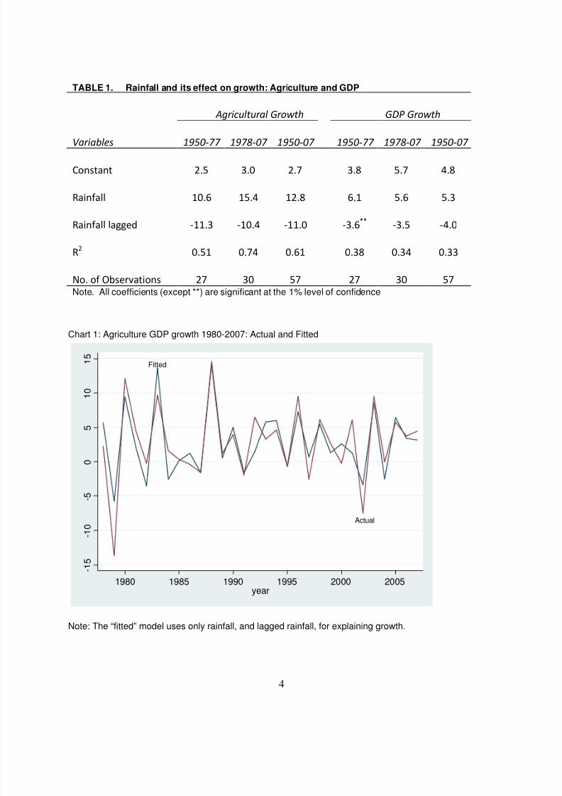
Table 1 documents the results for a model explaining agricultural and GDP growth. Surprisingly,

rainfall (lagged plus current) alone explains as much as 60 percent of the variation in the growth

of agricultural output. Decomposition of the data into two different time-periods, pre and post

1978, yields the same result. The last three years India has had exceptional agricultural output

growth averaging 4.7 % per year. The rainfall based prediction: 4.3 percent. For 2008/9, the

rainfall model predicts agricultural growth at a much lower 2 percent. The model for GDP growth

also works well; 40 percent of the variation in GDP growth is explained by rainfall alone. Chart 1

plots the fitted and actual value of agricultural growth for the period 1978-2007.

Industrial growth The reallocation model pre-supposes a movement of labor from agriculture to industry.

However, one of the striking stories about economic growth, and economic reforms in India, is



4

TABLE 1. Rainfall and its effect on growth: Agriculture and GDP

Agricultural Growth GDP Growth

Variables 1950-77 1978-07 1950-07 1950-77 1978-07 1950-07

Constant 2.5 3.0 2.7 3.8 5.7 4.8

Rainfall 10.6 15.4 12.8 6.1 5.6 5.3

Rainfall lagged -11.3 -10.4 -11.0 -3.6**

-3.5 -4.0

R2

0.51 0.74 0.61 0.38 0.34 0.33

No. of Observations 27 30 57 27 30 57Note. All coefficients (except **) are significant at the 1% level of confidence

Chart 1: Agriculture GDP growth 1980-2007: Actual and Fitted

Note: The “fitted” model uses only rainfall, and lagged rainfall, for explaining growth.

Fitted

Actual

- 1 5

- 1 0

- 5

0

5

1 0

1 5

1980 1985 1990 1995 2000 2005year



5

the lack-lustre performance of Indian industry . And this in large part explains the low rate of

GDP growth in India in the first five decades after independence. Even today, profits and money

making activity are viewed with contempt by many policy makers and most politicians.

Industrialists are constantly under suspicion. For most of the post economic reform period,

Indian industry has paid a considerably higher cost of capital than most of its competitors3. In

addition, the one advantage India ostensibly had, cheap labor, was reduced to zero (if not

negative) by both an overvalued exchange rate and restrictions on employers for hiring and

firing. All of these policies have contributed to India’s pitifully lower share of industry, compared

to an economy at its level of development and size. The figures are too stark to be missed: in

2006, industry’s share of GDP in India was only 26 percent; in China it was 22 percentage

points higher at 48 percent i.e. almost twice the size!

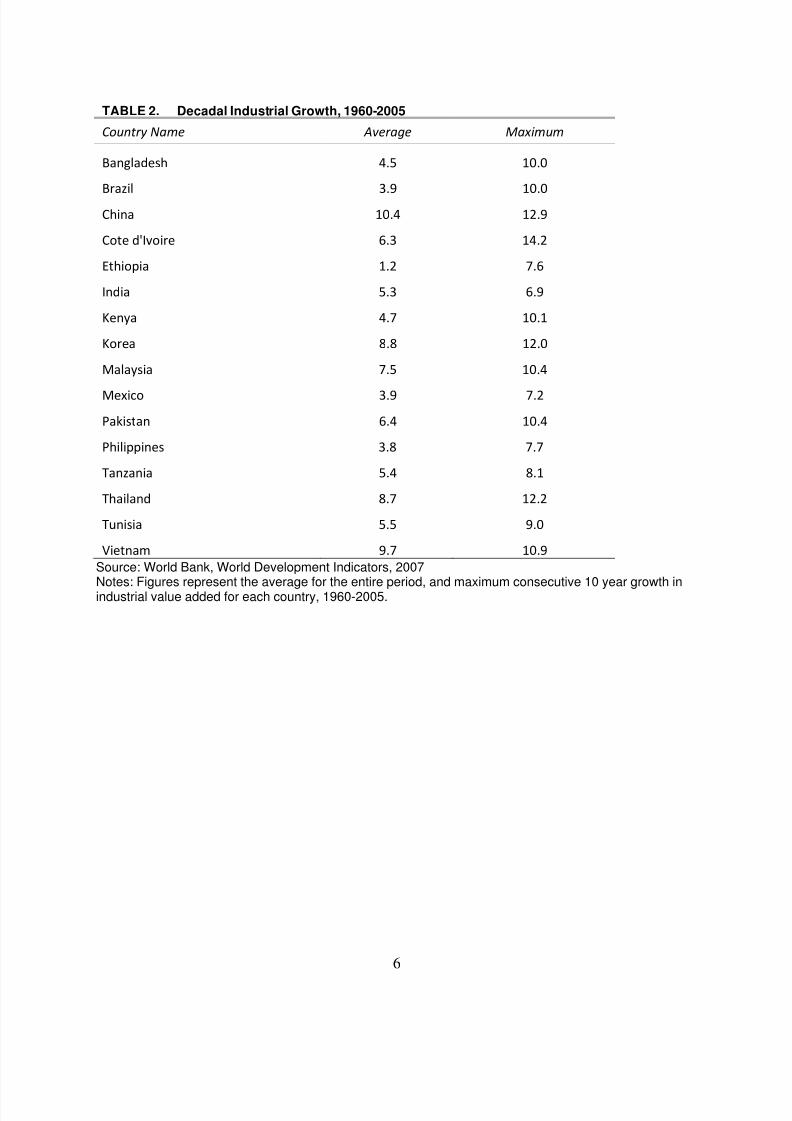
This low share is the result of low growth of industrial output. Table 2 reports the highest 10 year

moving average growth in industrial value added in selected countries. Data are till 2005 and

are revealing. The maximum 10 year average in China was 12.9 percent; the maximum ever

achieved in India, at 6.9 percent, is a figure almost half that of China. Out of 81 developing

countries4, India’s rank is 48. And several countries have exceeded India’s maximum of 6.9

percent decadal growth - Brazil, Ethiopia, Pakistan to name a few. Several countries have a

maximum industrial growth rate near double that achieved by India. India’s position has

improved in the last few years, but it is still revealing that India has never registered a decadal

industrial growth rate of above 7 percent.

Two policies affect industrial production greatly, and more than policies most often cited by

policy makers and/or experts. It is not labour reforms, nor reservations in the small scale sector,

nor the lack of effective bankruptcy laws, nor the lack of privatization, nor the public sector

character of industry that has made Indian industry a bad performer. All these good policies

matter, but not as much as a competitive exchange rate and competitive real interest rates. This

is examined next.

3In the last two years (2007 and 2008), Indian monetary policy has reverted back to very high real interest rates with

predictable consequences. See Section 4.4

Oil dependent countries and countries with population less than 1 million in 2006 are excluded; see Appendix I for

a list of the excluded countries.



6

TABLE 2. Decadal Industrial Growth, 1960-2005

Country Name Average Maximum

Bangladesh 4.5 10.0

Brazil 3.9 10.0

China 10.4 12.9

Cote d'Ivoire 6.3 14.2

Ethiopia 1.2 7.6

India 5.3 6.9

Kenya 4.7 10.1

Korea 8.8 12.0

Malaysia 7.5 10.4

Mexico 3.9 7.2

Pakistan 6.4 10.4

Philippines 3.8 7.7

Tanzania 5.4 8.1

Thailand 8.7 12.2

Tunisia 5.5 9.0

Vietnam 9.7 10.9

Source: World Bank, World Development Indicators, 2007Notes: Figures represent the average for the entire period, and maximum consecutive 10 year growth inindustrial value added for each country, 1960-2005.



7

Section 3 – Models of Growth

The study of growth determinants has been a growth industry for decades. Though there are

several factors that contribute to economic growth, the principal determinants are few. In identity

terms, economic growth is the sum of factor accumulation and productivity growth. Research

has centered on the decomposition of factor accumulation (the rate of return to different factors)

and the decomposition of productivity growth (technological change, efficiency of factor use).

Data on capital stock5 and employment growth can be used to estimate output per worker as a

function of capital per worker. This yields an elasticity of capital as 0.63. This is almost identical

to the elasticity found by Bhalla(2007a) for a large sample of developing countries for the time-

period 1950-2007, as well as close to the estimate (0.59) found for China by Hu and Khan.

Capital and labor force growth have stayed relatively constant for fifty years, and only lately has

capital growth spurted to record levels, and levels consistent with those observed in East Asian

economies at the time of their record growth, and at a level today somewhat higher than China.

This result means that factor accumulation is not an explanation for the 1980s growth

acceleration. Some of the popular assumed determinants of growth and inflation are examined

next.

Monetary Policy – Money Supply growth

The emphasis on money supply growth, both as a tool and as an indicator of monetary

tightening, has declined in most parts of the world. The data accompanying the bi-annual IMF

flagship product on growth and inflation, World Economic Outlook , has no information on money

supply (MS) growth. Curiously, in India, money supply (or non-food credit) growth still reigns

supreme in the minds of policymakers. All policy documents of the RBI, and policy

pronouncements, contain copious references to the level of MS growth, how it is missing its

target level (it has been solidly constant at 17 percent growth for the last 40 years), and how

deviations of MS growth from this target level are believed to be linked to inflation.

For example, in its Policy Review of July 2008, when the RBI unexpectedly raised the overnight

lending rates by 50 basis points, the RBI stated “It is necessary to moderate monetaryexpansion and plan for a rate of money supply growth in the range of around 17.0 per cent in

2008-09 in consonance with the outlook on growth and inflation so as to ensure macroeconomic

and financial stability in the period ahead”. In its press statement on the stance of monetary

policy three months later, on Oct. 24 2008 – this at a time when world economies and world

5See Appendix I for a discussion of data sources and construction.



8

financial markets had crashed and entered the sharpest downfall in real activity, ever - the RBI

stated “Non-food credit has posted a growth of 29 per cent on a year-on-year basis as of

October 10, 2008 which is well beyond the projected level of 20 per cent for 2008-09 ”.

(emphasis added). A large part of this excess was due to commodity price inflation that had

already been experienced, but in the (erroneous) year to year methodology adopted by the RBI,

this simple fact was missed. In contrast to this strong belief, no research document of the RBI

shows any significant statistical relationship of money supply growth to either economic growth,

or to inflation. Indeed, the research strongly supports the no link hypothesis.

However, Rangarajan (1998), former governor of the RBI, does argue for a strong link between

money supply growth and inflation. “The short-run elasticities of price with regard to money

supply works out to 0.271, while the long-run elasticity is close to unity (1.04).” (p.64) This is

likely the basis for the RBI’s consistent belief in the role of money supply in affecting inflation.

However, the Rangarajan equation was estimated with variables defined in terms of the log

values, and thus suffered from severe problems of co-integration. His equation (fn1, p.64) was:

Ln P = 2.963 -0.481*lnY + .271*lnM3 + 0.739*lnP(-1) + .147*DUM74 + .069*DUM80

R2 = .995, time-period of regression 1972-3 to 1990-1

What Rangarajan estimated is the familiar quantity theory of money model, with velocity

assumed to be constant. It follows from the equation MV =PY where M is the quantity of money,

P the price level, and Y is real output. Moving P to the left hand side yields the monetarist

equation.

If the equation holds in levels, it should hold in log changes, and in the latter, co-integration

problems are considerably lessened, if not removed. The equation to be estimated, therefore, is

P’ = aM’ + bY’ + additional variables

where the prime (‘) indicates log percentage change.

Re-estimating the Rangarajan equation with the latest available data (1999 base) for the time-

period 1972-1990, one obtains



9

Ln P = 0.81 -0.20*lnY + .35*lnM3 + 0.41*lnP(-1) + .10*DUM74 + .01*DUM80

R2 = .9973, time-period of regression 1972-3 to 1990-1; t-statistic on M3 coefficient = 12.04

The new data suggests that the short-run elasticity of price with money is even higher, at .35

rather than 0.27. Re-estimating the quantity theory of money model in log changes, one

obtains:

P’ = 5.7 - 0.67*Y’ + .33*M3’ + 4.52*DUM74 + 3.39*DUM80

R2 = .48, time-period of regression 1972-3 to 1990-1; t-statistic on M3 coefficient = 0.65

The explanatory power of the model is substantially reduced, and the significance of the money

supply coefficient, from being the most significant explanatory, drops to complete insignificance

(significant at the 52 percent level of confidence).

Results for the money supply model, for different time-periods, are reported in Table 3. A

surprising, and major, result is that beginning in the 1980s, no matter what the specification (i.e.

what variables are included or excluded from the analysis), money supply growth has zero

effect on output growth. The same result holds for the twenty-two year period prior to 1973 . As

with output, so with inflation – money supply growth does not statistically matter. 6

Yet, with the addition of a mere 7 years of data for the 1970s (1973 to 1979), the regressions

for the entire 57 year period, 1950-2007, do show that money supply growth has a statistically

significant effect on growth, and inflation. It is perhaps this regression result which has led

Indian policy makers to constantly emphasize money supply growth. It is well known that in the

1970s there was stagflation around the world due to the large commodity price rise exaggerated

by the quadrupling in the price of oil in Oct. 1973 and the doubling in the price of oil in 1979. Themonetary accommodation of this price change leads to a strong correlation between inflation,

money supply growth and GDP growth in the 1970s. The fact that this correlation ceases to

appear for any period after or before lends strong support to the hypothesis that money supply

6See Bhalla(1981a) for one of the early estimations of the monetarist and Keynesian models for developing

countries, and Bhalla(1981b) for a detailed analysis of different models of inflation for India.



10

growth, in the broad observed ranges (2 to 21 percent) holds little information about inflation or

GDP growth in India.

While it may appear as if the volatility in money supply growth is large, it is actually the smallest

in India among all countries of the world, and smallest by a large margin. Among 165 countries

for the period 1980-2007, volatility (standard deviation of money supply growth) in India was 1.7

percent; the second lowest volatility was observed for USA at double this level, 3.4 percent, and

another large economy, China, had a rank of 34 at a volatility almost four times higher, 6.5

percent. The median volatility among all nations was 11.4 percent per annum, or about 7 times

higher than India.

The lack of statistical relevance of money supply growth has not prevented the government of

India, via the RBI, from initiating major monetary tightening moves on the basis of short-term

spikes in the inflation rate; these moves have not had any effect on inflation but have affected

long-term growth prospects, via the effect on interest rates (see below). The mid-1990s

monetary tightening (starting in early 1995) is an important case in point, as has been the recent

2007 and 2008 tightening of monetary policy. In both instances, the policy was in response to a

surge in WPI inflation; in both instances, domestic demand, “overheating”, was considered the

real culprit. In both instances, the rise in inflation was imported. Thus, in both instances, policy

for constraining domestic inflation was in response to factors determining international inflation.

Some of the parallels. WPI inflation had moved to double digits in March 1994 from an average

of 7.7 percent in the preceding 12 months. In response, the RBI increased the CRR (cash

reserve ratio) by 1 percentage point to 15 percent, and call money rates doubled to 12 percent

plus by Jan. 1995.



11

TABLE 3. Money Supply and Fiscal Deficits: (non)-Effects on Growth and Inflation

Coefficient 1950-72 1980-07 1950-07

Dependent variable: GDP Growth

M3 Growth (lagged) -0.03 -0.08 0.20**

Inflation -0.06 -0.20 -0.24**

R2

0.45 0.53 0.46

Dependent variable: Inflation (GDP deflator)

M3 Growth (lagged) -0.20 0.32 0.48**

GDP Growth 0.48 -0.64* -0.60**

R2

0.26 0.31

1980-03 1980-03 1980-07

Dependent variable: GDP growth

Fiscal Deficit lagged (% of GDP) -0.23 -0.38* -.24

Real Interest Rate (lagged) -0.25*** -.38***

Currency Undervaluation (lagged) -.01* -.024***

R2

0.71 0.79 0.76

Notes:1: *Stars indicate the level of statistical significance; 1, 2, and 3 stars indicate significance at the 10%,

5%, and 1% level of significance, respectively.2. Other variables in the equation are rainfall, rainfall lagged and in growth equations, a dummy variable

for 1991, when applicable.



12

Table 4a documents the close relationship between domestic and world inflation7. In Table 3, it

was documented that the monetarist inflation model had an explanatory power (R 2) of only 25

percent. An alternate inflation model is to postulate that domestic inflation is a function of world

inflation and this inflation increases, or falls, with the movements in median world inflation. The

median inflation often represents different countries in different years. Between 1992 and 1996,

median world inflation fell by 4.5 percentage points; Indian inflation, GDP deflator, fell by

2.4 percentage points. Approximately the same decline is obtained for other inflation measures

like CPI. It also turns out that 1994 was a year of global inflation as well8. The world median

inflation rate in 1994 was 13.3 percent, and registered an acceleration of 3.5 percentage points

over 19939. The wholesale price inflation in India also peaked in 1994, but consumer price

inflation did not – and nor did the GDP deflator. The GDP deflator was not then available on a

quarterly basis, but data on CPI was, albeit with a 2 month lag 10. (Table 4b)

The close relationship between domestic and world inflation suggests that domestic

policymakers do not have the instruments to more than moderately affect the domestic inflation

rate – a phenomenon all to true in the present (2008) world inflation period. The response

coefficient of Indian inflation to median world inflation is around 0.7; if the undervaluation of the

US dollar is added to the equation, the coefficient for world inflation drops to 0.55, and the sign

on US undervaluation is negative i.e. as the US dollar gets undervalued (it becomes too cheap),

world inflation goes up. Indian undervaluation has an opposite, positive, effect on domestic

inflation, and its presence reduces the world inflation coefficient to 0.35. That is, the more the

Indian currency is undervalued (undervaluation has a negative sign), there is less domestic

inflation, ceteris paribus . This result is contrary to the assertion made by several Indian

economists and commentators (see Shah et. al. (2008 )) that exchange rate appreciation is

needed to lower inflation.

7

This is computed as the inflation recorded by the GDP deflator and is different for each year.8The dollar hit its cyclical low in March 1995, and this might have contributed to the connectedness of international

inflation in the mid 1990s. The present 2008 global inflation also follows a near identical pattern, and as discussed

below, Indian policymakers seemingly still design macro policy pertaining to inflation with the belief that India is a

closed economy. This may have something to do with the fact that most of the macro policy makers in India are

from the era of a closed economy.9

Note that this was not caused by the Mexican devaluation, which happened on Dec. 20, 1994.10

Since monetary policy works with long and variable lags, a month or two delay should not be a matter of much

concern. Thus, it is curious that monetary policy in India has been based on weekly year on year movements in the

wholesale price index.



13

The extraordinary events of 2008 confirm this strong relationship between world and domestic

inflation. In tandem, Indian inflation (WPI, CPI, GDP deflator) went up with world inflation; in

tandem, Indian inflation has come down. By end-Dec. 2008, world inflation was down close to

zero. In India, the three month average WPI inflation (seasonally adjusted and annualized) was

-4.9 percent; CPI inflation, 4.8 percent, and GDP deflator, -7.2 percent.

Very few variables can explain the pattern of inflation in India; money supply growth, a favorite

of Indian central bankers and policy makers, cannot explain much at all. But median inflation in

the world, along with currency undervaluation in the US and India, can explain close to 90

percent of Indian inflation for the last twenty years!

Fiscal Policy

The second major belief of Indian policymakers (besides money supply growth) has been that

fiscal deficits, again in the broad ranges observed in India, matter, and matter for both

growth and inflation. This belief is consistent with belief worldwide (a consistency not observed

with money supply growth). Hence, a favorite policy recommendation, for both developed and

developing economies, has been: “reduce the fiscal deficit”. This can be observed in any of the

hundreds of documents produced by the IMF, the Ministry of Finance, or the RBI. Unlike money

supply growth, there is plausible economic reasoning behind this recommendation. The benefits

of deficit reduction are supposed to be manifold: greater efficiency in production, less losses in

government undertakings, and less “crowding out” of private investment. Indeed, institutions like

the European Union, and the Maastricht treaty, have partly been based on the notion that

government deficits matter a lot. An important reason why fiscal deficits can matter is the strong

theoretical relationship between fiscal deficits and real interest rates, at least in a closed

economy. High fiscal deficits mean a higher than “normal” real interest rate for private investors

– the crowding out thesis.



14

TABLE 4a: Domestic and World Inflation

Dependent Variables: Inflation (GDP deflator)

1950-80 1980-07

Variables 1 2 1 2 3

World Inflation 0.32* 0.38** 0.68*** 0.35*** 0.28***

Undervaluation USA 0.12 -0.07*** -0.07***

Undervaluation India -0.05 0.013*** 0.014***

R2

0.14 0.27 0.69 0.77 0.87

*Stars indicate the level of statistical significance; 1, 2, and 3 stars indicate significance at the 10%,5%, and 1% level of significance, respectively.

Note. Model 3, 1980-07 has a dummy variable for crisis year 1991.

Chart 2: World (median) and Indian inflation (GDP deflator)

Notes: The median country is likely to be different for each year.

World

India

0 . 0

5 . 0

1 0 . 0

1 5 . 0

1980 1985 1990 1995 2000 2005year



15

TABLE 4B. Inflation Indicators, fiscal years

1950-2008 (in %)

GDP deflator CPI WPI

Decades

1950-59 1.9

1960-69 6.0 6.4 6.3

1970-79 8.1 7.5 8.6

1980-89 8.6 9.2 8.0

1990-99 8.7 9.5 8.1

2000-07 4.3 4.7 5.1

Years

1991 13.8 13.9 13.8

1992 9.1 11.8 10.0

1993 9.6 6.4 8.3

1994 9.3 10.2 12.6

1995 9.4 10.2 8.0

1996 6.8 9.0 4.6

1997 6.4 7.2 4.4

1998 8.2 13.2 6.0

1999 4.6 4.7 3.3

2000 3.4 3.2 7.1

2001 3.0 5.2 3.7

2002 4.0 4.0 3.4

2003 4.2 2.9 5.5

2004 5.3 4.6 6.5

2005 4.8 5.3 4.4

2006 5.6 6.7 5.4

2007 4.5 5.5 4.7

2008* 1.5 6.0 1.0

*Estimate for fiscal year 2008/9



16

Despite some strong underpinnings, cross-country regressions have yet to find more than a

mixed result of the effect of fiscal deficits on economic growth. No matter what the specification,

the empirical effect of fiscal deficits, if and when statistically significant , is found to be less than

0.1 i.e. for each 1 percentage point reduction in the fiscal deficit, growth is found to be 0.1

percentage point higher. Period. This means that as a country moves from a fiscal deficit of 4 %

of GDP to zero, it will only add about 0.4 % to annual GDP growth. A revolution in economic

policy and only 0.4 % of extra GDP growth? This ‘extra growth’ may seem “reasonable” for

developed countries whose potential GDP growth is around 3 percent. Even then it is a small

effect for an economic, and policy, revolution. But the total fiscal revolution effect is

insignificantly small for developing countries, whose average GDP growth in the last few years

has been above 5 percent per annum. It is very likely that open capital markets have muted any

effect that fiscal deficits might ordinarily have had on interest rates.

But these are cross-country results based on certain assumptions which may not apply to a

time-series analysis of Indian deficits. There are several statistical problems in estimating the

effect of fiscal deficits on GDP growth in India. First, there is a very close correspondence

between the doubling of fiscal deficits from 5 to 10 percent of GDP (prior and post 1980) and the

acceleration in growth rate (again, post 1980). Second, is the low volatility in the level of these

deficits; for most of the period post 1980, consolidated fiscal deficits of India have hovered

around 8 % of GDP. So it is virtually impossible to obtain any significant relationship between

fiscal deficits and GDP growth. Indeed the relationship observed is often of the wrong sign, that

is negative. Given that fiscal deficits have a negative sign, a negative coefficient means that

more the (negative) level of the fiscal deficit, higher is GDP growth. This, is, of course, the

Keynesian expectation, and the expectation today when the world is faced with a global

slowdown and a Keynesian stimulus is considered necessary for battling the slowdown.

However, this relationship is not statistically sound, or significant (Table 3).

An additional reason for the lack of significance of the fiscal deficit is the “structure” of these

deficits. The link between fiscal deficits and interest rates in India is the opposite to that whichprevails in most parts of the world. McKinnon had emphasized the importance of “financial

repression” - the term was meant to emphasize the distorting effects of extremely low, and

highly negative, real rates of interest. In India, financial “repression” or extreme distortion has

meant too high administered and therefore too high interest rates the government pays to

borrow. The too high interest payments on these borrowings means larger than “necessary”



17

expenditures and therefore too high fiscal deficits. This is discussed in detail in Bhalla(2000) –

“Financial Sector Policies in India – Apne Pair pe Apni Kulhadi” which means “axing one’s own

feet”.

The Indian policy on fiscal deficits (until 1999) was as follows. The Ministry of Finance (MoF) set

a very high assured interest rate on savings for depositors in “small savings” funds11.

Administered interest rates were kept high in the 1990s, despite rapidly falling inflation, because

of the government’s preoccupation, and belief, and one fully endorsed by the RBI’s tight

monetary policy, that GDP growth of 7 % meant overheating and higher future inflation.

Perceived future inflation had to be reduced, and this could only be done via more monetary

tightening. So administered interest rates, in the form of interest rates on “small savings”

administered by different state governments, were kept at a nominal level of 12.5 percent or

higher.

The method of financing the fiscal deficit – the states and centre freed from the worry of raising

funds for deficit financing because depositors were paid an inordinately high rate of interest -

most likely made the case that fiscal deficits were the result of administered and high interest

rates, rather than fiscal deficits being the cause of high interest rates. Even with inflation at the

trend level of 8 percent (this prior to the period after 1995 when inflation averaged 5 percent)

meant a real rate on deposits of 4.5 percent; adding the normal spread of 3.5 percent meant

real lending rates averaging 8 percent, among the highest in the world and considerably higher

than rates prevailing in the developed world or in East Asia.

These high borrowing rates caused government interest payments to rise, which, ceteris

paribus , caused the fiscal deficit to rise. In the mid to late nineties, interest payments accounted

for more than 50 percent of the fiscal deficit, reaching a peak of 98 percent in 2007 (see Chart

3). In the 1980s, interest payments were only 2 percent of GDP versus near 5 percent of GDP in

the late 1990s. The share of interest payments in the consolidated fiscal deficit of India has

been higher than 60 percent in every year since the mid-1990s and in the last few years has

11 When I came back to India in 1996, I was struck by the abnormally high rates of interest in India andalso surprised that nobody was talking about it. It was Montek who set me on the right path by advisingme to look at the structure of “small savings”. I wrote about a dozen articles on the subject; in Feb. 1999,the Ministry of Finance started cutting these rates and two years later, in 2001, the RBI(2001) ratified themove by recommending that interest rates on small savings deposits be set close to the rates ongovernment borrowings. This suggests that Montek knew about the problem, and the solution, longbefore others “discovered” both.



18

been approaching 100 percent. Thus, high interest rates have caused high deficits and this has

resulted in lower GDP growth; see below.

Investment and the role of interest rates

Perhaps reflecting its central planning past, and perhaps reflecting the philosophical orientation

of the policy makers, monetary policy in India has been of the quantitative kind – quantity

targets of money supply, non-food credit growth. The overnight lending rate of the central bank

(the repo rate) was introduced in 2000. Despite a near decade of practice, the policy and market

discussions of monetary policy have been oriented towards the quantity of money, and not its

price. Reflecting this (misguided) policy emphasis, most writing on Indian growth has also

ignored this important dimension. Panagariya makes no mention of interest rate policy in his

study of Indian growth. Ditto for most other contributors in the debate e.g. Rodrik-Subramaniam,

De Long and Kohli. Virmani does discuss the role of interest rates but empirically finds a zero

effect, most likely because he (erroneously) uses the WPI deflator as a measure of inflation. 12

Acharya(2006) does mention the role of interest rates in affecting investment, but it is one of

several variables mentioned. “The link between real interest rates and private investment is

likely to be embedded in a more complex causal story of investment behavior which includes

financial intermediation, `animal spirits’ or confidence and uncertainty” (p.89) Perhaps it is this

view that has prevented the RBI from realizing that monetary policy has been restrictive towards

investment in crisis year 2008. Inflation has fallen by 10 percentage points (GDP price deflator

or WPI falling from above 10 percent to zero or below in the space of just six months) and the

repo rate by just 4 percentage points.

Contrary to this (malign!) neglect, empirically, the level of real interest rates has been or is a

significant determinant of investment, and therefore GDP growth. Table 5a shows regressions

of (lagged) real interest rate on the investment rate, and on GDP growth (Table 5b).

Regressions are estimated for the time-periods 1950-2007, 1980 to 2007 and 1993 to 2007.

The results are striking, and informative, especially for the post-1992 period. Real interest rates

have a significant effect with each 1 percentage point rise leading to a decline in the rate of

growth of investment by 2 to 3 percentage points.

12For reasons unknown, both the major economic departments in the government of India, the Ministry of Finance

and the RBI, have used, and continue to use, the wholesale price index (WPI) inflation measure as a “correct”

indicator of inflation. It is well known, both in the case of India and elsewhere, that the WPI is a misleading

indicator and should not be used for policy direction. For example, in the mid-1990s when the RBI tightened policy

on the basis of rising WPI inflation, both the deflator and CPI showed inflation in 1994 to be equal to or below the

1991-1993 average; WPI inflation was 2 percentage points higher (Table 4b).



19

Chart 3 : The Importance of Interest Payments

For GDP growth, the impact is around 0.3 to 0.6 i.e. each one point rise in the real interest rateleads to a decline in GDP growth of 0.3 to 0.6 percentage points. The regressions also include

the effects of currency undervaluation, a variable whose construction, and importance, is

examined below.

To be sure, there are other factors affecting investment rates in India - global financial crises

and in particular the East Asian crisis. However, empirically, no effect is observed; insertion of a

dummy variable for the years 1997 to 1999 results in an insignificant coefficient (t statistic of -

.19) for a regression run for the post-reform period 1993 to 2007. If the regression is run for theperiod 1980-2007, the t-stat for the East Asian crisis improves to -1.65 with a magnitude of -1.94

and significant only at the 11 percent level.

% Share of Interest Payments in Fiscal Deficit

% Share of Interest Payments in GDP

2 0 . 0

4 0 . 0

6 0 . 0

8 0 . 0

1 0 0 . 0

2 . 0

3 . 0

4 . 0

5 . 0

6 . 0

7 . 0

1980 1985 1990 1995 2000 2005year



20

TABLE 5a: Determinants of Investment (% of GDP)

Coefficient of

Constant

Lagged

Undervaluation

Lagged Real

Rate R

2

1950-07

Model 1 28.3 -0.09*** 0.80

1980-07

Model 1 27.9 -0.065*** 0.58

Model 2 30.5 -0.088*** -0.66** 0.69

1993-07

Model 1 27.3 -0.13*** 0.42

Model 2 32.9 -0.11*** -1.33*** 0.80

TABLE 5b: Determinants of GDP growth

Coefficient of

ConstantLagged

UndervaluationLagged Real

RateR

2

1980-07

Model 1 6.7 -0.013** 0.59

Model 2 8.0 -0.023*** -0.33*** 0.75

1993-07

Model 1 6.6 -0.055*** 0.43

Model 2 9.27 -0.04*** -0.62*** 0.89*Stars indicate the level of statistical significance; 1, 2, and 3 stars indicate significance at the 10%,5%, and 1% level of significance, respectively.



21

Chart 4 plots GDP growth rate in India since 1993 with the real interest rate lagged one period

and plotted in an inverted manner. 13 There is an extremely close correspondence between the

two, including a matching of the turning points (the correlation coefficient is -0.83). For example,

real interest rates increased by 400 basis points from 3.4 percent in 1993 to 7.2 percent in 1996,

and peaked in 2000 at 7.3 percent. The growth rate declined from 7.8 percent in 1994 to 4.1

percent in 1997, and bottomed at 4 percent in 2000. The acceleration in GDP growth (8.4

percent vs. 3.8 percent the previous year) started in 2003/4, ostensibly because of good

weather; agricultural growth topped 10 percent that year. In the background, is the clue of real

interest rates. In the years 1999 to 2003, the government had proceeded to cut administered

interest rates on deposits from 12.5 percent to 8 percent. With inflation staying broadly constant

at 4 percent, this meant a 400 to 500 basis point decline in real interest rates; and this has been

the major, and only identifiable, contributor to the growth acceleration of recent years.

Chart 4: The (lagged) effect of interest rates on GDP growth

13Lending rates are proxied by the average yield on government securities; the SBI prime lending rate gives

qualitatively the same results. In both cases, the real rate is obtained by subtracting inflation as measured by the

GDP deflator. In regression equations, the one year lagged value of the real rate is used as a determinant.

Lagged Real Interest Rates

GDP Growth 0 . 0

2 . 0

4 . 0

6 . 0

8 . 0

4 . 0

5 . 0

6 . 0

7 . 0

8 . 0

9 . 0

1993 1995 1997 1999 2001 2003 2005 2007year



22

Exchange rate policy

Balassa was one of the original, and leading, proponents of export-led growth for developing

countries. In short-hand, export-led growth is “currency undervaluation” and the empirical proof

of this is the success story of Japan, East Asia, China etc. In several papers 14 I have argued

about the importance of the exchange rate in determining economic growth – more specifically,

about how under-valuation of currencies (the East Asia tested growth model) helps a country to

achieve a faster growth rate. If under-valuation of currency causes growth, then the question

arises: how does one measure under-valuation? There are several methods and these are

discussed in detail in Bhalla(2007a, 2008b). The most popular method is to either take a basket

of currencies, or the US dollar, and derive inflation adjusted exchange rates with respect to a

“base” year (hereafter the IMF definition of real exchange rates). This is also the method

followed by the RBI for the Indian rupee, with 1993/94 as the base year.

A major drawback of the IMF/RBI method is that the base or “equilibrium” year needs to be

defined ex-ante. An alternate method is to use the procedure first suggested, and employed, by

Balassa(1964). This method regresses the real exchange rate on per capita income, and

deviations represent the degree of over and under valuation. Non-linear estimation techniques

were used in Bhalla(2007a), Second Among Equals …(hereafter SAE) to estimate a non-linear

version of the Balassa formulation; an elongated S-shaped relationship between real exchange

rates and per capita income was estimated.15

The channel of influence of currency undervaluation on GDP growth is via investments. An

undervalued currency directly leads to greater profitability of investments (both domestic and

FDI), a higher investment rate, and therefore higher growth. Indirectly, higher FDI can lead to

greater efficiency of investments and therefore higher growth. Striking confirmation of this

simple model of investments is obtained from the regressions reported in Table 5. No matter

what the time-period (before or after 1980), or specification (with or without (lagged) real interest

rates), the impact of undervaluation is large – each 10 percent increase in undervaluation leads

to almost a 1 percent increase in the investment rate. In a reduced form growth model, thesame significant relationship holds; each 10 percent increase in undervaluation leads to a 0.2

percentage point increase in GDP growth.

14See (e.g. Bhalla(1997, 2003, 2007a) for a detailed discussion of the different theoretical and empirical approaches

to measuring the mis-alignment of currencies.15

The results according to the SAE measure of undervaluation have considerably greater statistical significance than

the alternate IMF measure or the “traditional” alternatives proposed by Johnson-Ostry-Subramaniam(2007).



24

Chart 5b: Partial regression plot of currency undervaluation and GDP growth, 1993-2007

Chart 5c: Partial regression plot of real interest rates and GDP growth, 1993-2007

Notes: See Model 2, Table 5b for details of the regression equation; both currency undervaluation and real interest

rates are entered with a 1 period lag.

2007

2006

2000

2001

2003

2005

1999

1998

2004

1997

19942002

1996

1995

1993

- 2

- 1

0

1

2

e ( y g d p k | X

)

-40 -20 0 20 40e( uvl | X )

coef = -.04039563, (robust) se = .01321022, t = -3.06

1995

2005

2004

2007

1994

1993

1999

2006

1996

2003

20021998

1997

2001

2000 - 3

- 2

- 1

0

1

2

e ( y g d p k | X

)

-4 -2 0 2 4e( rrgsecl | X )

coef = -.62016498, (robust) se = .08579753, t = -7.23



25

Section 4: Growth Puzzles Explained

Puzzle 1: Why did growth accelerate in the early 1980s?

The first puzzle of Indian growth is the near identical levels of economic growth before, and

after, the reforms of 1991/92.16 The 1991 reforms were major: in a short period of time, the

reforms achieved the following: devaluation of the rupee by 20 percent, reduction in the peak

tariff rate 300 percent to 110 percent, elimination of the Monopolies and Restrictive Trade

Practices act, a structural adjustment loan from the International Monetary Fund. Starting in

1994, the Indian economy felt the full impact of these reforms as growth accelerated to above 7

percent for three consecutive years. Agricultural growth fluctuations had caused GDP growth to

often grow above 7 % (e.g. in 1964, 1967, 1975 etc.); however, this was the first time such

growth had occurred without a snap back from a preceding drought year. But soon the economy

stuttered and registered an average growth rate of only 5.1 percent for the period 1997-2002.

Hence, the equivalence of average decadal growth rates, 1980-99 and 1990-99 – and the

research on growth equivalence.

Such research only started post 2000. Until then, most economic research on India 17 had

highlighted the important causative role of 1991 reforms in accelerating India’s growth. The

common assumption among researchers was that since India had a major economic crisis in

1990-91, and since growth had clearly jumped in the following years, it was unlikely that growth

in the eighties was anywhere near the post-reform growth. The first paper to highlight the

constancy of India’s growth rate for the 1980s and 1990s was Bhalla et. al., Start of India’s

Decade, Feb 200018.

“The Indian economy has been growing at a steady rate of 5.5% to 6.5% for the last twentyyears – a fact ignored by most analysts. Excluding the crisis year of 1991-92, the lowest GDPgrowth rate observed in Indian economy has been 3.0% witnessed in 1982-83. In spite of continuous economic reforms, there has been no acceleration in the growth rate . This presentsa key question for both analysts and policy makers. (Bhalla et al 2000, p.2, emphasis added).

Table 6 reproduces the table from that paper, with updates for the period post 2000. As theIndia’s Decade paper noted, no matter what the indicator - GDP growth, money supply growth,

16See Virmani(2005) for a comprehensive listing, with dates, of the various reforms initiated in India since 1970.

17See Bhalla(1997), Virmani(1997), and Ahluwalia and other papers in the Bajpai-Sachs volume (1999).

18It is possible that other articles highlighted this fact before; the important point is about the nature of research and

how “collective” its mind-set is i.e. until Bhalla(2000) (or another paper), no researcher had pointed to the lack of

acceleration of growth post the 1991 reforms.



26

fiscal deficits, industrial production - non-overlapping three year averages suggested that the

Indian economy was an unchanging constant (until at least a full 12 years after the reforms).

TABLE 6. Hindu Constants and the Constancy of growth rate 1980-2002

Growth in

GDPIndustrial

ProductionM3

Share of Fiscal

Deficit/GDP

Real Interest

Rates*

Decades

1950-59 3.3

1960-69 4.4 8.8

1970-79 2.9 4.0 17.4 -3.8

3 Year Averages

1980-82 5.6 4.6 16.1 -5.5 -3.3

1983-85 5.6 8.0 17.5 -6.9 1.5

1986-88 6.4 8.4 17.4 -7.8 3.9

1989-92 4.3 5.6 17.6 -6.9 2.7

1993-95 5.9 5.1 17.4 -6.0 2.0

1996-98 6.1 8.6 16.2 -5.2 5.0

Data after the "India Decade" article

1999-01 5.9 5.2 17.8 -5.8 5.7

2001-03 5.8 5.2 15.4 -5.5 5.8

2004-07 9.1 9.1 17.9 -3.7 2.1

1992-95 6.2 7.1 17.0 -5.7 2.3

1997-03 5.3 4.8 17.3 -5.9 6.1

2003-07 8.9 8.7 17.0 -3.8 2.6

Notes. * Defined as the difference between the weighted government securities rate and inflation asmeasured by the GDP deflator.

Since this early 2000 article, a healthy debate has developed on the issue of value-added (or

not) of economic reforms. One view - as argued by De-Long, Rodrik-Subramaniam, and Kohli

- holds that there was indeed some, albeit vague, policy shift in the early 1980s when Mrs.

Indira Gandhi was returned to power. Some of her earlier policies were: nationalization of the



27

banking sector in 1969; raising the marginal income tax rate to 98 percent in 1971 as part of her

“garibi hatao ” or “poverty removal” campaign; via a constitutional amendment, inserting the term

“socialist” in the constitution in 1976; imposing a national emergency in 1974, and forcing a

pliant parliament and judiciary to authorize her dictatorial interventions. All of this, but when she

came back to power in 1980, argue the pre-reform growth advocates, she had a change of

heart, became pro-business, winked at the industrialists, and caused the Indian growth rate to

accelerate to 5.5 percent from the prevailing “Hindu rate of growth” of 3.5 percent per annum.

DeLong was the first to state that the 1991 economic reforms were not all that growth

accelerating; that the reforms post 1984 were responsible. (His explanation fails to explain the

1980-1984 acceleration).

“Yet the timing of the growth acceleration suggests an earlier start for the current Indian boomunder the government of Rajiv Gandhi… There’s lack of hard evidence to support the view thatin the absence of the second wave of reforms in the 1990s, it is unlikely that the rapid growth ofthe second half of the 1980s could be sustained.”

Rodrik-Subramaniam are the most forceful in concluding that the big-scale and big-item Indian

trade reforms of the early 1990s had little role to play in inducing a growth acceleration; rather,

the transition to a higher growth path had been achieved more than a decade earlier; not 1984

as argued by De-Long but 1980, the year Mrs. Gandhi came back to power.

“India’s growth transition began in the early 1980s rather than after the crisis of 1991. Theperformance of the 1980s appears to have been triggered by a perception on the part of theprivate sector that the government’s attitude toward it had changed, a perception that wassubsequently (in the mid-to-late 1980s), mildly validated by piecemeal reforms of the industriallicensing system. The attitudinal shift signaled by the Congress governments in the 1980selicited a large productivity response”.

Kohli (2006) echoed the Rodrik-Subramaniam conclusion about changed attitudes and Mrs.Gandhi’s “wink-wink” industrial policy as being the major instrument for change and

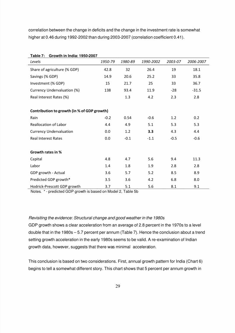
acceleration. But as Table 7 makes clear, contrary to Kohli’s forceful assertions, the rate of

capital formation stayed the same in 1980s as before.



28

“Indira Gandhi herself shifted India’s political economy around 1980 in the direction of a stateand business alliance for economic growth. This change was not heralded loudly and has oftenbeen missed by scholars …. The[se] changes emerged in fits and starts…the changes werenevertheless profound; they involved a shift from left-leaning state intervention that flirted withsocialism, to right-leaning state intervention…. big capital, understood these changes prettyclearly, expressing their satisfaction by investing more and helping India’s economy grow

rapidly.” Kohli(2006, p.1255)

Virmani and Panagariya represent the opposite view i.e. that while there was growth

acceleration in the 1980s, the 1991 reforms were the real thing. Both maintain that some

reforms made the 1980s acceleration possible but that large scale reforms were needed in the

1990s; both assert that the 1980s growth was unsustainable, as “proven” by the economic crisis

of 1990-91.

Panagariya: “The difference between the reforms in the 1980s and those in the 1990s is that theformer were limited in scope and without a clear road map whereas the latter were systematicand systemic.” (, p. ?)

Virmani: “The increase in investment in machinery and the greater availability and use of higherquality equipment imports were important factors in the acceleration in growth during this phase[1980-1991]” (2006, p.72)

None of the above debate participants really address the issue of the growth slowdown in the

mid-1990s i.e. why did economic growth acceleration post reforms die out after a mere three

years? The recent papers by Bosworth-Collins-Virmani(2006), and Bosworth-Collins(2006) in

their comparative study of India-China growth, also fail to answer this question. Acharya(2006)

explicitly addresses this question and concludes: “The year 1997 was a watershed, which rang

in the end of the economic party. In particular, three marker events occurred within a six month

period to check the momentum of growth” (p.61, emphasis added). These three events were:

political instability in March (end of Deve Gowda government), the East Asian financial crisis in

July and the implementation of the Fifth Pay Commission report in September. The link for

Acharya is higher fiscal deficit leading to lower investment – political uncertainty, financial crisis

etc. lead to higher fiscal deficits, crowding out, therefore lower investment and therefore lower

growth. Empirically, the effects are negligible. It is the case that a decline in the fiscal deficit is

correlated with an increase in the investment rate. But this association was there in the growth

slowdown decade 1992 to 2002 and the growth acceleration years 2003 to 2007. Indeed, the



29

correlation between the change in deficits and the change in the investment rate is somewhat

higher at 0.46 during 1992-2002 than during 2003-2007 (correlation coefficient 0.41).

Table 7: Growth in India: 1950-2007

Levels 1950-79 1980-89 1990-2002 2003-07 2006-2007

Share of agriculture (% GDP) 42.8 32 26.4 19 18.1

Savings (% GDP) 14.9 20.6 25.2 33 35.8

Investment (% GDP) 15 21.7 25 33 36.7

Currency Undervaluation (%) 138 93.4 11.9 -28 -31.5

Real Interest Rates (%) 1.3 4.2 2.3 2.8

Contribution to growth (in % of GDP growth)

Rain -0.2 0.54 -0.6 1.2 0.2

Reallocation of Labor 4.4 4.9 5.1 5.3 5.3

Currency Undervaluation 0.0 1.2 3.3 4.3 4.4

Real Interest Rates 0.0 -0.1 -1.1 -0.5 -0.6

Growth rates in %

Capital 4.8 4.7 5.6 9.4 11.3

Labor 1.4 1.8 1.9 2.8 2.8

GDP growth - Actual 3.6 5.7 5.2 8.5 8.9

Predicted GDP growth* 3.5 3.6 4.2 6.8 8.0

Hodrick-Prescott GDP growth 3.7 5.1 5.6 8.1 9.1

Notes. * - predicted GDP growth is based on Model 2, Table 5b

Revisiting the evidence: Structural change and good weather in the 1980s

GDP growth shows a clear acceleration from an average of 2.8 percent in the 1970s to a level

double that in the 1980s – 5.7 percent per annum (Table 7). Hence the conclusion about a trendsetting growth acceleration in the early 1980s seems to be valid. A re-examination of Indian

growth data, however, suggests that there was minimal acceleration.

This conclusion is based on two considerations. First, annual growth pattern for India (Chart 6)

begins to tell a somewhat different story. This chart shows that 5 percent per annum growth in



30

India prior to the 1980s wasn’t that unusual; several times the two-year growth average (two

years because of the periodic bad-rain good rain agricultural cycle) had exceeded 5 percent in

the period prior to the 1980s. Second, the conclusion about a large acceleration or breakout in

GDP growth seems to be based on a comparison of 1980s vs. 1970s. But for most countries,

Note: Bars are shown for the years between 1950 and 1979 when GDP growth was above 5 percent.

1970s is a bad “benchmark” and most countries would anyway show a marked acceleration in

the 1980s. The 1970s were a turbulent period for the world economy, with food, commodity and

oil prices sky-rocketing and bringing in their wake stagflation. The 1980s were a lot better in

terms of lower oil prices and lower world inflation. India was not immune to these events. GDP

growth in the 1950s and 1960s averaged 4 percent; the 1970s average was only 2.8 percent.

So the real acceleration in the 1980s is about 1.7 percentage points (5.7 minus 4 percent).

4

6

8

10

12

0

2

Percent per year

1950 1960 1970 1980Year

Chart 6 GDP growth above 5% - Not that unusual



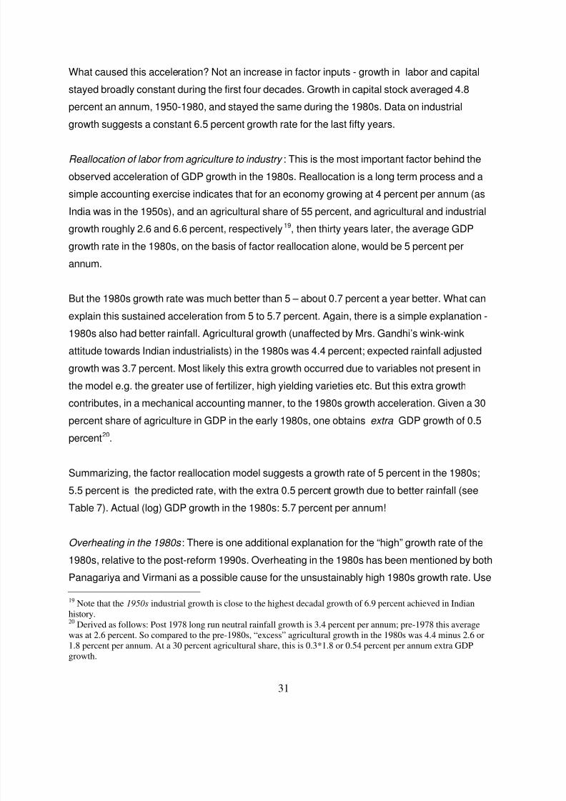
31

What caused this acceleration? Not an increase in factor inputs - growth in labor and capital

stayed broadly constant during the first four decades. Growth in capital stock averaged 4.8

percent an annum, 1950-1980, and stayed the same during the 1980s. Data on industrial

growth suggests a constant 6.5 percent growth rate for the last fifty years.

Reallocation of labor from agriculture to industry : This is the most important factor behind the

observed acceleration of GDP growth in the 1980s. Reallocation is a long term process and a

simple accounting exercise indicates that for an economy growing at 4 percent per annum (as

India was in the 1950s), and an agricultural share of 55 percent, and agricultural and industrial

growth roughly 2.6 and 6.6 percent, respectively19, then thirty years later, the average GDP

growth rate in the 1980s, on the basis of factor reallocation alone, would be 5 percent per

annum.

But the 1980s growth rate was much better than 5 – about 0.7 percent a year better. What can

explain this sustained acceleration from 5 to 5.7 percent. Again, there is a simple explanation -

1980s also had better rainfall. Agricultural growth (unaffected by Mrs. Gandhi’s wink-wink

attitude towards Indian industrialists) in the 1980s was 4.4 percent; expected rainfall adjusted

growth was 3.7 percent. Most likely this extra growth occurred due to variables not present in

the model e.g. the greater use of fertilizer, high yielding varieties etc. But this extra growth

contributes, in a mechanical accounting manner, to the 1980s growth acceleration. Given a 30

percent share of agriculture in GDP in the early 1980s, one obtains extra GDP growth of 0.5

percent20.

Summarizing, the factor reallocation model suggests a growth rate of 5 percent in the 1980s;

5.5 percent is the predicted rate, with the extra 0.5 percent growth due to better rainfall (see

Table 7). Actual (log) GDP growth in the 1980s: 5.7 percent per annum!

Overheating in the 1980s : There is one additional explanation for the “high” growth rate of the

1980s, relative to the post-reform 1990s. Overheating in the 1980s has been mentioned by bothPanagariya and Virmani as a possible cause for the unsustainably high 1980s growth rate. Use

19Note that the 1950s industrial growth is close to the highest decadal growth of 6.9 percent achieved in Indian

history.20

Derived as follows: Post 1978 long run neutral rainfall growth is 3.4 percent per annum; pre-1978 this average

was at 2.6 percent. So compared to the pre-1980s, “excess” agricultural growth in the 1980s was 4.4 minus 2.6 or

1.8 percent per annum. At a 30 percent agricultural share, this is 0.3*1.8 or 0.54 percent per annum extra GDP

growth.



32

of econometric techniques (Hodrick-Prescott filter, Table 7) does suggest that growth was

above trend in the 1980s (trend estimated at 5.1 percent, and close to the reallocation model)

and at trend in the 1990s (5.6 percent). A raw look at the growth data disguises this important

difference.

Puzzle 2: Why did growth not accelerate in the 1990s?

Responding to economic reforms, GDP growth did accelerate and averaged above 7.4 percent

in each of the three years 1994 to 1996. But this acceleration to potential had some unintended

consequences. The irony is that the government itself (or elements within it) did not believe that

the reforms it had instituted would increase the potential GDP growth rate to above 7 percent.21

In the mindset of the Indian politicians, and most policy makers, it was inconceivable that the

Indian economy could grow at East Asian growth rates; the doubling of the rate of growth above

Hindu rates of 3.5 percent was considered impossible; the 7 plus percent growth rate was

considered as an overheating phase deserving a strong policy response. Possibly it was the

crisis of 1991 that prevented policymakers from realizing that an expansion from 5.7 to 7.4

percent growth was the mildest of accelerations. When this acceleration coincided with global,

and domestic inflation, the RBI panicked and tightened monetary policy to an unprecedented

degree. Further, the RBI did not cut interest rates in response to the decline in worldwide, and

domestic, inflation in the mid to late 1990s. By keeping deposit rates at high double digit levels,

and inflation collapsing, the RBI ensured that real rates reached double digit levels. This caused

the growth to collapse, as documented in the previous section.

Puzzle 3: Why did growth accelerate so sharply 2003 onwards?

The new Congress government came to power in May 2004, after an agriculture induced robust

growth of 8.4 percent in 2003/4. During the preceding five years (excluding 2003/4), GDP

growth averaged only 5.3 percent per annum, about 0.3 percent per year less than the long-

term 1980s and 1990s average of 5.6 percent. With no growth friendly policy inputs during2004-2007, the economy continued to average 9 percent growth, a record by any yardstick.

21Why the Indian government would engineer far reaching reforms in order to panic when growth accelerated by

barely 1 to 1.5 percent per annum deserves deeper analysis.



33

In an eerie replay of the 1990s, there is a new controversy, this time about the dog that did bark.

No economic reforms and growth acceleration; what happened?22. Many, including several

economists, senior government officials, the Economist and the IMF have claimed that the

acceleration is proof of over-heating and growth much in excess of potential GDP growth of 7

percent. Others, e.g. Bhalla et. al.(2006), claim that there was a structural break in Indian

growth rate starting 2003, and that the potential GDP growth of India, without any additional

economic reforms, is close to 9 percent, a finding supported by statistical exercises like the

Hodrick-Prescott filter (see below).

Structural break in growth in 2003/4 – Decline in real interest rates the cause

In 1999, inflation had reached a low of 3.5 percent and the government took the first major step

towards interest rate reforms. Within a space of four years, government bond yields were at 5

percent, down from double digit plus levels of the late 1990s. In “normal” economies, such a

large decline in long-term real interest rates would ordinarily be headline news for several years.

Analysts would relate industrial growth, GDP growth, stock prices, to this mega event. After all,

in western economies, a mere 25 basis point change in interest rates is a momentous occasion.

So it is in several developing economies, including China.

This interest rate change is most likely a major cause for the marked increase in investment that

is observed for the 2003+ period. Savings rates had hovered around 25 percent the previous

decade (1993 to 2002) and investment rates had averaged the same. Since 2002, in just five

years, savings and investment rates have increased by 11 and 12 percentage points

respectively.

Industry has most likely been the biggest beneficiary of this lower interest rate regime. Growth in

industry rose at its fastest pace in 2004-2007. While industry grew at 8% for 2004-07,

manufacturing growth was strong at around 9.1%. The increase in GDP growth since 2002 is

the sharpest, and longest, in Indian history: a large 4 to 5 percentage point acceleration (neardoubling) to beyond 9 percent per annum. However, in an eerie replay of the mid 1990s,

skepticism remains. Most analysts, and economists, and especially the monetary authorities,

doubt the sustainability of this acceleration and feel that the economy is or has been in a

22At the time this paper was written (Oct. 2008), there is an unprecedented worldwide crisis, and the impact of this

crisis and world, and Indian growth rates, is highly uncertain. What is reported here are long-term trends.



34

substantial overheating phase. 23 The base case belief is that any growth rate above 6 to 7

percent per annum is not sustainable.

This skepticism suggests that India maybe sui generis . No policy maker, and very very few

analysts, have pointed to the decline in real interest rates as an important cause, let alone the

cause, for India’s growth acceleration. Lower real interest rates add to GDP growth, and a 500

basis point decline in real rates is enough to add somewhere between 1.5 to 3 percent extra

GDP growth (see Table 5b – coefficient of lagged real rates is in the range -0.3 to -0.6

depending on the time-period and specification). And higher GDP growth leads to higher

savings rates, and expectations of higher growth lead to an increase in investment rates. This is

what explains the jump in investment rates, savings rates, and GDP growth rates in the last five

years. And this change is structural, not cyclical.

Potential GDP growth in India at 8.5 percent plus

Various “models” of growth indicate that the potential GDP growth in India i.e. the rate at which

overheating is zero, is close to 8.5 percent plus. The assumptions and framework behind each

assessment, and forecast, is detailed below.

Method 1: Bosworth-Collins : In a study ending with 2004 data i.e. with only two years of 8.5

percent growth, Bosworth-Collins(p.19) state that “current rates of capital accumulation are

consistent with a GDP growth rate near 7 percent, but higher rates would require reductions in

the public sector deficit or increases in capital flows from abroad”. It is useful to infer what the

Bosworth-Collins “model” would state for Indian growth in 2008. Since 2004, capital growth has

increased to above 11 percent from an average of 7.5 percent in 2003-2004; and investment

and saving rates have increased by about 10 percentage points. Given a capital to growth

elasticity of 0.63, this increase in investment should result in an extra 2 to 2.5 percent growth.

Thus the new data would indicate that the Bosworth-Collins forecast of trend GDP growth in

2008 would be around 9 plus percent.

Method 2: Factor accumulation: An investment to GDP ratio of 36 to 38 percent implies that the

growth of capital stock is upwards of 10 percent per annum. Very rarely have investment rates

23How growth can be more than 2 % above expectations for 5 consecutive years, and still be transitory, is an issue

not addressed by the pessimists. See Bhalla et. al.(2006) for a detailed discussion about the likelihood that there was

a structural break in Indian growth around 2003/4.



35

jumped by 10 percentage points over three years (as has just happened in India) and then

reverted back in a hurry. This “episode” of increasing investment rates, and then stabilization

around 40 percent plus levels, is likely to occur over the next several years. Employment growth

has averaged more than 3 percent per annum recently. Assuming a lower rate of 2.5 percent,

and a capital share at 63 percent, expected GDP growth, with zero productivity growth, is 7.2

percent per annum. Total factor productivity growth over the last five years has averaged close

to 2 percent per annum (between 1.7 and 2.1 percent, various estimates). This method yields a

potential GDP growth estimate above 9 percent.

Method 3: Industrial growth estimates: Services presently account for close to 55 percent of

Indian GDP, industry 25 percent, and agriculture 20 percent. As documented earlier, there is no

time period when industry has averaged more than 7 percent growth (on a decadal basis). For

the last 4 years, industrial growth in India has averaged 8.7 percent. For the four year period

1999-2002, industrial growth was only 5 percent. It is reasonable to assume that industrial

growth in India will average 9 percent.24 If this happens, then the historical relationship between

services and industrial growth (arbitraged through the labor market) suggests that services will

grow by 10 percent. Average agricultural growth of 3 percent suggests that the potential GDP

growth in India is 8.4 percent per annum.

Method 4: Econometric techniques - the Hodrick-Prescott (HP) filter: There are several

sophisticated econometric techniques for estimating potential GDP growth. Chart 7 plots the HP

estimate and a simple 5 year average. The HP filter suggests a new plateau of growth around 9

percent.

24All forecasts are contingent upon a “neutral” world economy; short-term cycles, linking India to events and

economies abroad, are to be expected.



36

Note: Potential growth is according to the Hodrick-Prescott filter.

Method 5: Potential growth compared to China: In Bhalla(2007a) the growth rates for India andChina were forecast according to several methods. At present, India is ahead of China in terms

of both the growth rate of capital, and employment. In addition, an extra 0.3 percent per year

growth is likely for India (catch up effect) because China’s income is two and a half times that of

India. Further, India’s currency appreciation is likely to be about 3 to 5 percentage points less a

year than China’s – and therefore, the decline in currency undervaluation less. For 2008, China

enjoys a 2 percentage point lead in expected GDP growth. Combining all the three factors

(initial conditions, exchange rate change and investment levels) India’s growth rate should

exceed China’s by as early as 2010. This is a radically different forecast than that articulated byother experts e.g. the market-oriented BRIC’s report by Goldman Sachs (2003).

Additional support for this forecast is obtained by comparing the levels of total factor productivity

growth in the two economies, 1950 to 2007. (Table 8). Not surprisingly, TFPG growth in the two

countries has been very similar. For the entire 57 year period, China’s TFP growth has been 0.4

Long term Average = 6.4

Potential Growth

Average 5 year growth

2

4

6

8

10

1980 1990 2000 2010Year

Chart 7: Potential GDP Growth in India >= 8.5 percent



37

percent per year higher than India, and in the last five years, it has been 1.5 percent per annum

higher. Such divergences do not last for a long time, especially given the close match over the

long term. The expected convergence in TFPG rates is another reason to support the

hypothesis that Indian GDP growth will soon exceed China’s.

Financial crisis 2008 : The world is in the midst of a severe financial crisis and growth estimates

for 2008 have been lowered for all countries. The above analysis about potential GDP growth

suggests that while the level of GDP growth will be affected, India’s relative standing as one of

the fastest growing economies in the world will, or should not, be affected. In addition, there is

the forecast that India’s GDP growth will exceed that of China. In a globalized world, countries

are affected by global events to a much larger degree than anticipated or imagined. But this

does not mean that domestic policy is unlikely to have any effect. As has been documented

throughout this paper, evidence suggests that Indian policy makers have misused instruments

for misunderstood economic crises. If this path is continued, then the Indian economy will suffer

more than fundamentals suggest; if forward-looking policy initiatives replace the rear-view

policies that have been followed, then India could achieve its potential on a sustained basis.

Table 8 Total Factor Productivity Growth, India-China, 1950-2007

China India

1950-1980 1.96 1.23

1980-2002 2.4 3.04

1950-2002 2.2 1.98

2003-2007 5.34 3.84

1950-2007 2.56 2.14Note: Total factor productivity growth calculated on the basis of a pooled

Time-series cross country model; coefficient of capital = 0.52. See Bhalla(2009b)For details, see Bhalla(2009b).



38

Section 6: Conclusions

This paper has attempted to put the Indian growth, and inflation, story of the last 60 years in

perspective. The known determinants of growth and inflation were examined in detail. There are

two “new” explanations for the much discussed, and much-hyped, growth acceleration in the

1980s. Reallocation from agriculture to industry resulted in the potential growth rate being as

high as 5 percent; good weather added a few tenths to overall GDP growth rate. The sharp rise

in real interest rates, induced by very tight monetary policy at a time of falling inflation rates in

the mid to late 1990s resulted in industrial (and GDP) growth being killed before it reached its

potential. The reversal of this interest rate hike, and reduction to realistic and competitive levels

during 1999-2002, is a major reason for the miraculous growth acceleration observed starting

2003. Aiding and abetting this process of an economy moving towards a new and higher

potential GDP growth of around 9 percent were two factors; the maintenance of an increasingly

competitive exchange rate since 1993/9425, and the development and expansion of the middle

class.26

The Indian interest rate story helps complete the circle and explain Indian growth puzzles.

Summarizing, unwarranted tight monetary policy, and much higher than warranted real interest

rates, brought the Indian economy crashing down from a potential GDP growth rate of 7.5

percent to less than 5 percent in the late 1990s. Reversal of this policy brought the economy

back to 7.5 percent; further decline in the level of undervaluation (from 13 percent overvaluation

in 1996 to 30 percent undervaluation in 2006) has added another 1 percentage point to GDP

growth; hence, a potential GDP growth in India of at least 8.5 percent per annum.

The second growth puzzle examined was the seemingly zero acceleration in economic growth

despite the largeness of the economic reforms introduced in 1991. In reality, a marked

acceleration in economic growth did follow the reforms, but the improvement fizzled to zero. The

proximate causes of the “miraculous” growth post 2002 was also investigated. The roots of this

acceleration are found not in the reforms of 1991 (some people have argued that but it is just

too far away to be credible)27

but in the monetary mishap of the mid 1990s. Simply put, the largeincrease in real interest rates post the tightening of monetary policy in 1995-1996 contributed to

25See Bhalla(2008b) for a detailed evaluation of the role of currency undervaluation in affecting growth in

developing countries.26

See Bhalla(2008c) for a detailed evaluation of the role of the middle class in affecting growth, and reforms, in

countries over the last 400 years.27

Montek makes a strong case for the gradualism of the reforms process but I suspect that even he thinks that 13

years for reforms to take effect is a stretch for gradualism!



39

growth in the 1990s to be no more than growth in the 1980s; a complete reversal of this

monetary policy led to the growth acceleration 2003/4 onwards.

References

Acharya, Shankar, (2002), “India’s Medium-Term Growth Prospects”, Economic and Political

Weekly , pp. 2897-2906, July 13, 2002.

Ahluwalia, S. Montek, (2002), “Economic reforms in India since 1991: Has gradualismWorked?”, Journal of Economic Perspectives 16(3), 67-88.

Balassa, B. (1964) “The Purchasing Power Parity Doctrine: A Reappraisal.” Journal of Political Economy 72: 584–96.

__________ (1978) “Exports and Economic Growth: Further Evidence.” Journal of Development Economics 5 (2): 181–89.

Bhalla, Surjit S. (1981a) "India's Closed Economy and World Inflation", Chapter 5 in W.R. Clineand Associates, World Inflation and the Developing Countries, Brookings Institution,Washington, DC, 1981.

_________(1981b) "The Transmission of Inflation into Developing Countries", Chapter 3 in W.R.Cline and Associates, World Inflation and the Developing Countries, Brookings Institution,Washington, DC, 1981,pp. 52-101.

_________(1997a), “Economic Freedom and Growth Miracles: India is Next”, paper preparedfor a panel discussion on South Asia: The Next Miracle?, World Bank-IMF Annual Meeting,Hong Kong 1997, September 18, 1997.

_________1997b), “Freedom and Economic Growth: A Virtuous Cycle?”, in Democracy’sVictory and Crisis: Nobel Symposium 1994 ed. Axel Hadenius, Cambridge University Press,1997.

_____________(1999a), “Chinese Mercantilism: Currency Wars and How the East was Lost”,ICRIER Discussion Paper, March 1999.

____________ (1999b), “Time for Monetary Blackmail”, Economic Times , October 26.

____________(2000) “Financial Sector Policies in India – Apne Pair pe Apni Kulhadi ”, Chapter2 in Surjit S.Bhalla (ed.) New Economic Policies for New India, Proceedings of an ICSSRConference, Hari Haran Press, New Delhi, February

____________(2001) “In the Interest of India”, Business Standard , January 20.



40

____________(2002) “Trade, Growth and Poverty: Re-examining the Linkages.” Paperpresented at World Bank-ADB, “Fourth Asia Development Forum,” Seoul, Korea(November).

__________ (2006) Mid-Year Review of the Economy 2006-2007: India at a Structural Break ,

India International Center, New Delhi, Oct. (with Rohit Chawdhary and Tirthatanmoy Das)

__________ (2007a) Second Among Equals: The Middle Class Kingdoms of India and China.Washington: Peterson Institute of International Economics (May).

__________ (2007b) “There Are No Growth Miracles.” Paper presented at the InternationalMonetary Fund, Washington (August).

__________ (2008a) “Economic Development and the Role of Currency Undervaluation”, The Cato Journal , vol. 28, #2, Spring/Summer, p.313-340

_________ (2009a) UnderAppreciated Growth: Why “Competitive” Exchange Rates Matter

Washington: Peterson Institute of International Economics, forthcoming.

_________ (2009b) The Middle Class Kingdoms of China and India Washington: PetersonInstitute of International Economics, forthcoming.

Bhalla, Surjit, S., Chawdhry, Rohit, and, Mookerjee, Arindom, (2000), “Start of India’s Decade”,Developing Trends , Oxus Research & Investments, Vol. 4, No. 1&2, February 24, 2000.

Bosworth, Barry P. and Susan M. Collins (2006), “Accounting for Growth: Comparing China andIndia”, Brookings Institution.

Bosworth, Barry P., Susan M. Collins and Arvind Virmani (2006), “Sources of Growth in theIndian Economy”, Indian Policy Forum

Chandhok, H.L., and, The Policy Group, (1990), India Database, The Economy, Annual TimeSeries Data, Volume I & II.

DeLong, J. Bradford, (2001), “India Since Independence: An Analytic Growth Narrative,” in DaniRodrik, ed., Modern Economic Growth: Analytical Country Studies, July 2001.

Economic and Political Weekly Research Foundation, (2002), National Accounts Statistics ofIndia, 1950-51 to 2000-01, Fourth Edition, July 2002.

Foster, D. Andrew, and, Rosenzweig, R. Mark, (2003), “Agricultural Productivity Growth, RuralEconomic Diversity, and Economic Reforms: India, 1970-2000”, paper prepared for the D. GaleJohnson Memorial Conference, October 25, 2003.

Hu and Khan



41

Johnson, S.; Ostry, J. D.; and Subramanian, A. (2007) “The Prospects for Sustained Growth inAfrica: Benchmarking the Constraints.” IMF Working Papers 07/52. Washington:International Monetary Fund (March).

Joshi, Vijay and I.M.D. Little, (1994), India: Macroeconomics and Political Economy: 1961-91,Washington, DC: World Bank.

Mooley, D.A., Parthasarathy, B., Kumar, Rupa, K., Sontakke, N.A., Munot, A.A., and,Kothawale, D.R. (2003), “IITM Indian regional/subdivisional Monthly Rainfall data set (IITM-IMR)”, India Meteorological Department, www.tropmet.res.in/pub/data/rain/iitm-imr-readme.txt.

Nehru, V. and A. Dhareshwar (1993), “A New Database on Physical Capital Stock: Sources,Methodology and Results”, Revista de Analisis Economiico , Vol 8, pp 3-59

Panagariya, Arvind, (2004), “India in the 1980s and 1990s: A Triumph of Reforms”, IMF WorkingPaper WP/04/43, March 2004.

Reserve Bank of India (RBI), (2001), Report of the Expert Committee to Review the System of

Administered Interest Rates and Other Related Issues 2001 , Y V Reddy Chairman

Reserve Bank of India (RBI), (2003), Handbook of Statistics on the Indian Economy 2002-03,CD-ROM

Robinson, Sherman, 1971, “Sources of Growth in Less-Developed Countries: A Cross-SectionStudy”, Quarterly Journal of Economics 85 :391-408.

Rodrik, Dani, and, Subramanian, Arvind, (2004a), “From “Hindu Growth” to Productivity Surge:The Mystery of the Indian Growth Transition”, Draft, March 2004.

Rodrik, Dani, and, Subramanian, Arvind, (2004b), “Why India Can Grow at 7 Per Cent a Year or

More: Projections and Reflections”, Economic and Political Weekly , Vol. XXXIX No. 16, pp.1591-1596, April 17, 2004.

Samuelson, P. A. (1964) "Theoretical Notes on Trade Problems." Review of Economics and Statistics 46: 145–54.

Ajay Shah – exchange rate pass through article

Virmani, Arvind, (2004a), “India’s Economic Growth: From Socialist Rate of Growth to Bhartiya

Rate of Growth”, ICRIER Working Paper No. 122, February 2004.

Virmani, Arvind, (2004b), “Sources of India’s Economic Growth: Trends in Total Factor

Productivity”, Working Paper No. 131, ICRIER, May 2004.



Appendix I

Rainfall

Rainfall data has been obtained from www.tropmet.res.in. Monthly data on rainfall for a network

of rain gauge stations has been collected since the middle of the 19

th

century. As the websitestates:

The monthly (January – December) area weighted rainfall series for each of the 29meteorological subdivisions have been prepared by assigning the district are as the weight foreach rain-gauge station in that subdivision. Similarly assigning the subdivision area as theweight to each of the subdivisions in the region, area weighted monthly rainfall series areprepared for Homogeneous regions of India as well as for all India”.

The rainfall index was constructed as follows: For each month, and for each rainfall station, thestandard deviation was computed. The weighted average of these standard deviations for the

four months, June through September, is the index. Different aggregations were attempted, but

none proved as “explanatory” as this average of four month series.

Capital Stock

Nehru-Dhareshwar(1993) construct a capital stock series, on a uniform basis, for over ninety

countries for the period 1950-90. Refer to SAE, 28

Data on labor force

Access to National Sample Survey (NSS) Employment and Unemployment survey yields

estimates of employment according to three different definitions: usual status (usually one

month) , weekly status and daily status. The international norm is weekly status, and is the one

chosen here. The 1983 and 1993/4 surveys are used to derive employment growth for the

decade, and the 1993 and 1999, and 2004/5 surveys for employment growth post 1993. For

years prior to 1983, the labor force growth as obtained from World Bank, World Development

Indicators is used and grafted on to the estimate of employment in 1983.

28None of the results presented here are qualitatively affected by the choice of the capital stock series. Further, it

h ld b d d h i d h hi i l i l k d l i i i i l i / l i f

http://www.tropmet.res.in/



110IndianEconomicGrowth1950-2008

Documents

Transcript of 110IndianEconomicGrowth1950-2008