11. Oligopoly - Bergische Universität Wuppertal · In perfect competition, monopoly, and...
46
| 04.07.2017 | Prof. Dr. Kerstin Schneider| Chair of Public Economics and Business Taxation | Microeconomics| Chapter 11 Slide 1 | 11. Oligopoly Literature: Pindyck and Rubinfeld, Chapter 12 Varian, Chapter 27
Transcript of 11. Oligopoly - Bergische Universität Wuppertal · In perfect competition, monopoly, and...

| 04.07.2017 | Prof. Dr. Kerstin Schneider| Chair of Public Economics and Business Taxation | Microeconomics| Chapter 11 Slide 1 |
11. Oligopoly
Literature: Pindyck and Rubinfeld, Chapter 12
Varian, Chapter 27

| 04.07.2017 | Prof. Dr. Kerstin Schneider| Chair of Public Economics and Business Taxation | Microeconomics| Chapter 11 Slide 2 |
Chapter Outline
• Oligopoly
• Quantity Competition
• Price Competition
• Competition versus Collusion: The Prisoner‘s Dilemma

| 04.07.2017 | Prof. Dr. Kerstin Schneider| Chair of Public Economics and Business Taxation | Microeconomics| Chapter 11 Slide 3 |
Oligopoly
• Properties
– Small number of firms.
– The products may or may not be differentiated.
– Barriers to market entry.
• Example
– Automobiles
– Steel
– Aluminum
– Petrochemicals
– Electrical Equipment
– Computers
| 04.07.2017 | Prof. Dr. Kerstin Schneider| Chair of Public Economics and Business Taxation | Microeconomics| Chapter 11 Slide 4 |
Oligopoly
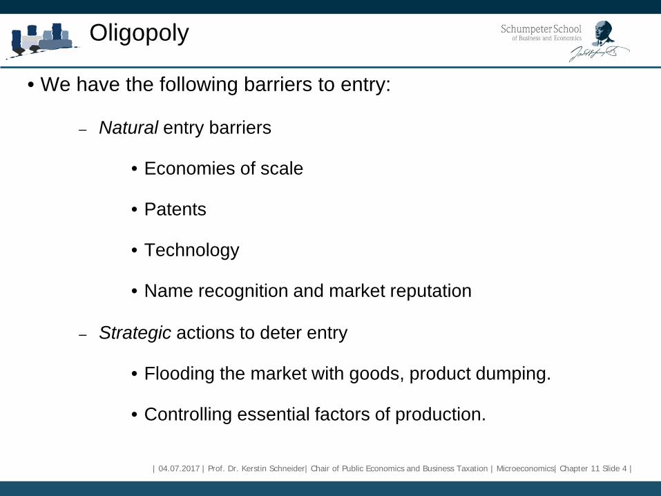
• We have the following barriers to entry:
– Natural entry barriers
• Economies of scale
• Patents
• Technology
• Name recognition and market reputation
– Strategic actions to deter entry
• Flooding the market with goods, product dumping.
• Controlling essential factors of production.

| 04.07.2017 | Prof. Dr. Kerstin Schneider| Chair of Public Economics and Business Taxation | Microeconomics| Chapter 11 Slide 5 |
Oligopoly
• Equilibrium for an oligopolistic market
– In perfect competition, monopoly, and monopolistic competition,
the producers do not have to take into account the response of
their rival‘s choice of output and price.
– However, in the case of an oligopoly, producers must take into
account their rival‘s response when choosing output and prices.

| 04.07.2017 | Prof. Dr. Kerstin Schneider| Chair of Public Economics and Business Taxation | Microeconomics| Chapter 11 Slide 6 |
Oligopoly
• Equilibrium for an oligopolistic market
– Definition of a market equilibrium
• When a market is in equilibrium, firms are doing the best
they can and have no reason to change their prices or
output levels.
• All firms set prices or output based partly on strategic
considerations regarding the behavior of their respective
competitors.
Nash Equilibrium: Set of strategies or actions in which each
firm does the best it can given its competitors‘ actions.

| 04.07.2017 | Prof. Dr. Kerstin Schneider| Chair of Public Economics and Business Taxation | Microeconomics| Chapter 11 Slide 7 |
Oligopoly
• The Cournot Model
– Duopoly
• Market in which two firms compete with each other.
• Homogeneous good.
• Each firm treats the output of its competitors as fixed.
• All firms decide simultaneously how much to produce

| 04.07.2017 | Prof. Dr. Kerstin Schneider| Chair of Public Economics and Business Taxation | Microeconomics| Chapter 11 Slide 8 |
Firm 1‘s Output Decision
MC1
50
MR1(75)
D1(75)
12.5
If Firm 1 thinks that Firm 2 will produce 75 units, its demand curve, D1(75), is shifted to the left by this amount.
Q1
P1
D1(0)
MR1(0)
If Firm 1 thinks Firm 2 will produce nothing, its demand curve, labeled D1(0), is the market curve.
D1(50)
MR1(50)
25
If Firm 1 thinks that Firm 2 will produce 50 units, its demand curve, D1(50), is shifted to the left by this amount.

| 04.07.2017 | Prof. Dr. Kerstin Schneider| Chair of Public Economics and Business Taxation | Microeconomics| Chapter 11 Slide 9 |
Oligopoly
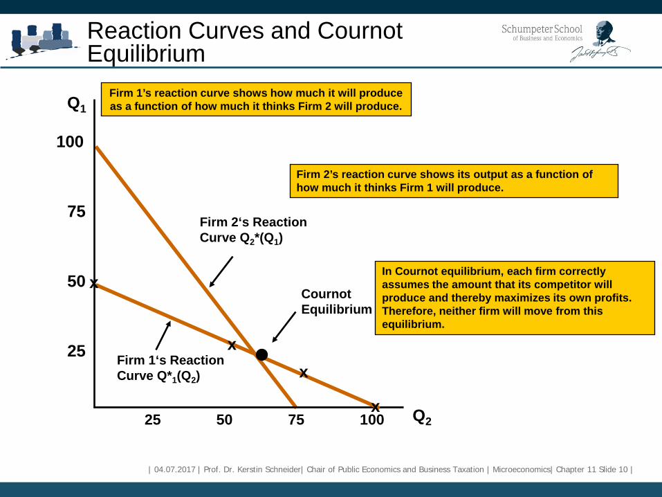
• Reaction curve:
– Relationship between a firm’s profit-maximizing output and the
output level it thinks its competitor will produce. Firm 1’s profit-
maximizing output is thus a decreasing schedule of how much
it thinks Firm 2 will produce.
| 04.07.2017 | Prof. Dr. Kerstin Schneider| Chair of Public Economics and Business Taxation | Microeconomics| Chapter 11 Slide 10 |
Reaction Curves and Cournot Equilibrium
Firm 2‘s Reaction Curve Q2*(Q1)
Firm 2’s reaction curve shows its output as a function of how much it thinks Firm 1 will produce.
Q2
Q1
25 50 75 100
25
50
75
100
Firm 1‘s Reaction Curve Q*1(Q2)
x
x x
x
Firm 1’s reaction curve shows how much it will produce as a function of how much it thinks Firm 2 will produce.
In Cournot equilibrium, each firm correctly assumes the amount that its competitor will produce and thereby maximizes its own profits. Therefore, neither firm will move from this equilibrium.
Cournot Equilibrium

| 04.07.2017 | Prof. Dr. Kerstin Schneider| Chair of Public Economics and Business Taxation | Microeconomics| Chapter 11 Slide 11 |
Duopoly Example
• An example of Cournot equilibrium
– Duopoly: two firms facing the following market demand
curve P = 30 – Q, where Q is total production of both
firms (i.e. Q = Q1 + Q2 )
– Suppose also that MC1 = MC2 = 0
The Linear Demand Curve

| 04.07.2017 | Prof. Dr. Kerstin Schneider| Chair of Public Economics and Business Taxation | Microeconomics| Chapter 11 Slide 12 |
Duopoly Example
• An example of Cournot equilibrium
– Firm 1‘s reaction curve
1 1 1Total revenue : R (30 )PQ Q Q= = −
122
11
1211
30
)(30
QQQQQQQQ
−−=
+−=
The Linear Demand Curve

| 04.07.2017 | Prof. Dr. Kerstin Schneider| Chair of Public Economics and Business Taxation | Microeconomics| Chapter 11 Slide 13 |
Duopoly Example
• An example of Cournot equilibrium
1 1 1 1 2
1 1
1 2
2 1
30 20
Firm 1's reaction curve15 1 2
Firm 2's reaction curve 15 1 2
MR R Q Q QMR MC
Q Q
Q Q
= ∂ ∂ = − −= =
= −
= −
The Linear Demand Curve

| 04.07.2017 | Prof. Dr. Kerstin Schneider| Chair of Public Economics and Business Taxation | Microeconomics| Chapter 11 Slide 14 |
Duopoly Example
• An example of Cournot equilibrium
― Firm 1‘s reaction curve:
1 1 21
1 2
Cournot equilibrium15 1 2(15 1 2 ) 10
2030 10
Q Q Q QQ Q QP Q
= − − ⇔ = =
= + == − =
The Linear Demand Curve

| 04.07.2017 | Prof. Dr. Kerstin Schneider| Chair of Public Economics and Business Taxation | Microeconomics| Chapter 11 Slide 15 |
Duopoly Example
Q1
Q2
Firm 2‘s Reaction Curve 30
15
Firm 1‘s Reactions Curve
15
30
10
10
Cournot Equilibrium
The demand curve is P = 30 – Q, and both firms have zero marginal cost.

| 04.07.2017 | Prof. Dr. Kerstin Schneider| Chair of Public Economics and Business Taxation | Microeconomics| Chapter 11 Slide 16 |
Duopoly Example
Profit maximization with collusion
𝑅𝑅 = 𝑃𝑃𝑃𝑃 = 30 − 𝑃𝑃 𝑃𝑃 = 30𝑃𝑃 − 𝑃𝑃2
𝑀𝑀𝑅𝑅 =𝜕𝜕𝑅𝑅𝜕𝜕𝑃𝑃 = 30 − 2𝑃𝑃
𝑀𝑀𝑅𝑅 = 0 = 𝑀𝑀𝑀𝑀, 𝑖𝑖𝑖𝑖 𝑃𝑃 = 15 𝑎𝑎𝑎𝑎𝑎𝑎 𝑀𝑀𝑅𝑅 = 𝑀𝑀𝑀𝑀

| 04.07.2017 | Prof. Dr. Kerstin Schneider| Chair of Public Economics and Business Taxation | Microeconomics| Chapter 11 Slide 17 |
Duopoly Example
Collusion curve
• Q1 + Q2 = 15.
― Gives all the output combinations of Q1 and Q2 for
which the total profit is maximized.
• Q1 = Q2 = 7.5.
― Smaller production quantity and higher profits in
comparison to Cournot equilibrium.
Profit maximization with collusion

| 04.07.2017 | Prof. Dr. Kerstin Schneider| Chair of Public Economics and Business Taxation | Microeconomics| Chapter 11 Slide 18 |
Duopoly Example
Firm 1‘s Reaction Curve
Firm 2‘s Reaction Curve
Q1
Q2
30
30
10
10
Cournot Equilibrium 15
15
Competitive Equilibrium (P = MC, Profit = 0)
Collusion Curve
7.5
7.5
Collusive Equilibrium
For the firm, the best solution is collusion; the next best solution is Cournot equilibrium, after that is competitive equilibrium, i.e., P = MC, Profit = 0.

| 04.07.2017 | Prof. Dr. Kerstin Schneider| Chair of Public Economics and Business Taxation | Microeconomics| Chapter 11 Slide 19 |
First Mover Advantage- The Stackelberg Model
• Assume that we have two duopolists:
– A firm can set its output before other firms do.
– MC = 0.
– The market demand is P = 30 – Q, where Q = total amount
produced.
– Suppose Firm 1 sets its output first; then Firm 2, after observing
Firm 1’s output, makes its output decision.

| 04.07.2017 | Prof. Dr. Kerstin Schneider| Chair of Public Economics and Business Taxation | Microeconomics| Chapter 11 Slide 20 |
First Mover Advantage- The Stackelberg Model
• Firm 1
– In setting output, Firm 1 must consider how Firm 2 will react.
• Firm 2
– Takes Firm 1’s output as fixed and, accordingly, determines its
production quantity using the Cournot reaction curve: Q2 = 15 -
1/2Q1.

| 04.07.2017 | Prof. Dr. Kerstin Schneider| Chair of Public Economics and Business Taxation | Microeconomics| Chapter 11 Slide 21 |
First Mover Advantage- The Stackelberg Model
• Firm 1 chooses Q1 so that its marginal revenue equals its marginal cost of zero:
𝑀𝑀𝑅𝑅 = 𝑀𝑀𝑀𝑀,𝑀𝑀𝑀𝑀 = 0, 𝑐𝑐𝑐𝑐𝑎𝑎𝑐𝑐𝑐𝑐𝑐𝑐𝑐𝑐𝑐𝑐𝑎𝑎𝑐𝑐𝑐𝑐𝑐𝑐 𝑀𝑀𝑅𝑅 = 0
• Recall Firm 1’s revenue is:
𝑅𝑅1 = 𝑃𝑃𝑃𝑃1 = 30𝑃𝑃1 − 𝑃𝑃12 − 𝑃𝑃2𝑃𝑃1

| 04.07.2017 | Prof. Dr. Kerstin Schneider| Chair of Public Economics and Business Taxation | Microeconomics| Chapter 11 Slide 22 |
First Mover Advantage- The Stackelberg Model
• By inserting the reaction curve of Firm 2 for Q2 we get
1 1 1 1
1 2
15
0 15 und 7.5
MR R Q Q
MR Q Q
=∂ ∂ = −
= ⇒ = =
21 1 1 1 1
21 1
30 (15 1 2 )
15 1 2
R Q Q Q Q
Q Q
= − − −
= −

| 04.07.2017 | Prof. Dr. Kerstin Schneider| Chair of Public Economics and Business Taxation | Microeconomics| Chapter 11 Slide 23 |
First Mover Advantage- The Stackelberg Model
We conclude that
• Firm 1 produces twice as much as Firm 2.
• Firm 1 makes twice as much profit as Firm 2.
– Going first gives Firm 1 an advantage

| 04.07.2017 | Prof. Dr. Kerstin Schneider| Chair of Public Economics and Business Taxation | Microeconomics| Chapter 11 Slide 24 |
Price Competition
• In an oligopolistic market, the competition may consist of
choosing a price instead of a quantity.
• Bertrand model: Oligopoly model in which firms produce a
homogeneous good, each firm treats the price of its competitors
as fixed, and all firms decide simultaneously what price to
charge.

| 04.07.2017 | Prof. Dr. Kerstin Schneider| Chair of Public Economics and Business Taxation | Microeconomics| Chapter 11 Slide 25 |
Price Competition
• Let’s return to the duopoly example:
– Homogeneous Good
– Market demand is P = 30 – Q, with Q = Q1 + Q2.
– This time, however, assume that MC = €3 for both firms and
therefore MC1 = MC2 = €3.
Bertrand Model

| 04.07.2017 | Prof. Dr. Kerstin Schneider| Chair of Public Economics and Business Taxation | Microeconomics| Chapter 11 Slide 26 |
Price Competition
• in Cournot equilibrium:
− Now suppose that these two duopolists compete by
simultaneously choosing a price instead of a quantity.
Bertrand Model
1 2
€12 9
for both firms €81
PQ Qπ
== =
=

| 04.07.2017 | Prof. Dr. Kerstin Schneider| Chair of Public Economics and Business Taxation | Microeconomics| Chapter 11 Slide 27 |
Price Competition
• What price will each firm use, and how much profit will
each earn? (Hint: assume homogeneous products,
meaning that consumers will purchase only from the
lowest-price seller.)
• The Nash Equilibrium
― P = MC; P1 = P2 = €3
― Q = 27; Q1 = Q2 = 13.5
― Since P=MC, both firms earn zero profit.
Bertrand Model

| 04.07.2017 | Prof. Dr. Kerstin Schneider| Chair of Public Economics and Business Taxation | Microeconomics| Chapter 11 Slide 28 |
Price Competition
• Why shouldn‘t a firm set prices higher in order to
increase profits?
• How does the result in the Bertrand model differ from
that of the Cournot model?
• The Bertrand model shows the meaning of strategic
variables (price versus quantity produced).
Bertrand Model

| 04.07.2017 | Prof. Dr. Kerstin Schneider| Chair of Public Economics and Business Taxation | Microeconomics| Chapter 11 Slide 29 |
Price Competition
• Criticism
– When a firm produces homogeneous goods, it is more
common that it competes by the quantity produced rather
than the selling price.
– And, even if firms set prices equal to each other, what share
of total sales will go to each one?
• Eventually, the quantity produced by the two firms will
not be the same.
Bertrand Model

| 04.07.2017 | Prof. Dr. Kerstin Schneider| Chair of Public Economics and Business Taxation | Microeconomics| Chapter 11 Slide 30 |
Price Competition with differentiated Products
• Suppose we have the following:
– Two duopolists
– FC = €20
– VC = 0
Differentiated Products

| 04.07.2017 | Prof. Dr. Kerstin Schneider| Chair of Public Economics and Business Taxation | Microeconomics| Chapter 11 Slide 31 |
Price Competition
• Assume they face the same demand curve:
– Firm 1’s demand curve is Q1 = 12 - 2P1 + P2
– Firm 2’s demand curve is Q2 = 12 - 2P2 + P1
• P1 and P2 are the prices that Firms 1 and 2
charge, respectively.
• Q1 and Q2 are the resulting quantities that they
sell.
Differentiated Products

| 04.07.2017 | Prof. Dr. Kerstin Schneider| Chair of Public Economics and Business Taxation | Microeconomics| Chapter 11 Slide 32 |
Price Competition
• Choosing price and quantity – Assume both firms set prices at the same time:
1 1 1
1 1 1 22
1 1 1 1 2
Firm 1's profit : €20 (12 2 ) 20
12 -2 20
PQP P P
P P PP
ππ
π
= −= − + −
= + −
Differentiated Products

| 04.07.2017 | Prof. Dr. Kerstin Schneider| Chair of Public Economics and Business Taxation | Microeconomics| Chapter 11 Slide 33 |
Price Competition
• Choosing price and quantity Firm 1 assumes P2 to be fixed:
’ :
’ :
’ :
π
π
∂ ∂ = − + =
= +
= +
= =
-Firm 1 s profit maximizing price P P P
-Firm 1 s reaction curve P P
-Firm 2 s reaction curve P P
-P
1 1 1 2
1 2
2 1
12 4 0
3 1 4
3 1 4
4 12
Differentiated Products

| 04.07.2017 | Prof. Dr. Kerstin Schneider| Chair of Public Economics and Business Taxation | Microeconomics| Chapter 11 Slide 34 |
Choosing Prices in Collusive Equilibrium
• Set the price in a way such that both firms maximize their profits.
• If firms cooperatively set price they choose P = €6; 16π =

| 04.07.2017 | Prof. Dr. Kerstin Schneider| Chair of Public Economics and Business Taxation | Microeconomics| Chapter 11 Slide 35 |
Nash Equilibrium in Prices
Firm 1‘s Reaction Curve
P1
P2
Firm 2‘s Reaction Curve
€4
€4
Nash Equilibrium
€6
€6
Collusive Equilibrium

| 04.07.2017 | Prof. Dr. Kerstin Schneider| Chair of Public Economics and Business Taxation | Microeconomics| Chapter 11 Slide 36 |
Competition versus Collusion: The Prisoner‘s Dilemma
• Nash-equilibrium is a non-cooperative equilibrium.
• Cooperation would have led to higher profits.
• Why don‘t firms cooperate without explicity colluding? In
particular, if you and your competitor can both figure out the
profit-maximizing price you would agree to charge if you were to
collude, why not just set that price and hope your competitor will
do the same?

| 04.07.2017 | Prof. Dr. Kerstin Schneider| Chair of Public Economics and Business Taxation | Microeconomics| Chapter 11 Slide 37 |
Competition versus Collusion: The Prisoner‘s Dilemma
• Let‘s go back to our example:
1 2
2 1
€20 and €0
Firm 1's demand curve: 12 2
Firm 2's demand curve: 12 2
Nash Equilibrium: €4, €12
Collusion: €6, €16
FC VC
Q P P
Q P P
P
P
π
π
− = =
− = − +
− = − +
− = =
− = =

| 04.07.2017 | Prof. Dr. Kerstin Schneider| Chair of Public Economics and Business Taxation | Microeconomics| Chapter 11 Slide 38 |
Competition versus Collusion: The Prisoner‘s Dilemma
Possible pricing options and respective results:
• If they collude, both ask €6 and 𝜋𝜋 = €16.
• In Nash equilibrium:
[ ]
[ ]
-if €6 and €41 2-then 202 2 2
4 12 (2)(4) 6 20 €202- 201 1 1
6 12 (2)(6) 4 20 €41
P P
P Q
P Q
π
π
π
π
= =
= −
= ⋅ − + − =
= −
= ⋅ − + − =

| 04.07.2017 | Prof. Dr. Kerstin Schneider| Chair of Public Economics and Business Taxation | Microeconomics| Chapter 11 Slide 39 |
Payoff Matrix for a Pricing Game
Firm 2
Firm 1
Charge €4 Charge €6
Charge €4
Charge €6
€12, €12 €20, €4
€16, €16 €4, €20

| 04.07.2017 | Prof. Dr. Kerstin Schneider| Chair of Public Economics and Business Taxation | Microeconomics| Chapter 11 Slide 40 |
Competition versus Collusion: The Prisoner‘s Dilemma
• Both firms play in a non-cooperative game (a game in
which negotiation and enforcement of binding contracts is
not possible).
– Each firm optimizes profits given its decision and the
decision of its competitor (payoff matrix).
• Question
– Why do both firms set a price equal to €4, when they
could gain more profit with a price equal to €6?

| 04.07.2017 | Prof. Dr. Kerstin Schneider| Chair of Public Economics and Business Taxation | Microeconomics| Chapter 11 Slide 41 |
Competition versus Collusion: The Prisoner‘s Dilemma
• A classical example in game theory, called the prisoner’s
dilemma, illustrates the problem faced by oligopolistic firms.
| 04.07.2017 | Prof. Dr. Kerstin Schneider| Chair of Public Economics and Business Taxation | Microeconomics| Chapter 11 Slide 42 |
Competition versus Collusion: The Prisoner‘s Dilemma
• Scenario
– Two prisoners have been accused of collaborating in a crime.
– They are in separate jail cells and cannot communicate with
each other.
– Each has been asked to confess.

| 04.07.2017 | Prof. Dr. Kerstin Schneider| Chair of Public Economics and Business Taxation | Microeconomics| Chapter 11 Slide 43 |
Payoff Matrix for Prisoner‘s Dilemma
-5, -5 -1, -10
-2, -2 -10, -1
Prisoner A
Confess Don‘t confess
Confess
Don‘t confess
Prisoner B

| 04.07.2017 | Prof. Dr. Kerstin Schneider| Chair of Public Economics and Business Taxation | Microeconomics| Chapter 11 Slide 44 |
Payoff Matrix for Prisoner‘s Dilemma
Conclusion: Oligopolistic markets
• Collusion yields higher profits.
• Explicit, secret, and implicit agreements are all possible.
• If there is a price agreement, then there is a motivation to
deviate from this agreement.

| 04.07.2017 | Prof. Dr. Kerstin Schneider| Chair of Public Economics and Business Taxation | Microeconomics| Chapter 11 Slide 45 |
Concluding Remarks
• In an oligopolistic market, few firms account for most or all of the
production.
• In the Cournot model of oligopoly, firms make their output
decisions at the same time, each taking the other’s output as
fixed.
• In the Stackelberg model, one firm sets its output first.

| 04.07.2017 | Prof. Dr. Kerstin Schneider| Chair of Public Economics and Business Taxation | Microeconomics| Chapter 11 Slide 46 |
Concluding Remarks
• The Nash equilibrium concept can also be applied to markets in
which firms produce substitute goods and compete by setting
price.
• Firms can earn higher profits through price collusion (pricing
agreements made in private), however this is prohibited by
Antitrust laws.
• The prisoner‘s dilemma creates price rigidity in oligopolistic
markets.