11. Cramer Rao Bounds

11. Cramer Rao BoundsECE 830, Spring 2017

1 / 36

The Cramer-Rao Lower BoundThe Cramer-Rao Lower Bound (CRLB) sets a lower bound on thevariance of any unbiased estimator. This can be extremely usefulin several ways:

1. If we find an estimator that achieves the CRLB, then we knowthat we have found a “minimum variance unbiased estimator”(MVUE)!

2. The CRLB can provide a benchmark against which we cancompare the performance of any unbiased estimator. (Weknow we’re doing very well if our estimator is “close” to theCRLB)

3. The CRLB enables us to rule-out impossible estimators. Thatis, we know that it is physically impossible to find an unbiasedestimator that beats the CRLB. This is useful in feasibilitystudies.

4. The theory behind the CRLB can tell us if an estimator existswhich achieves the bound.

2 / 36

Estimator Accuracy

Consider the likelihood function p(x|θ) where θ is a scalarunknown (parameter).

We can plot the likelihood as a function of the unknown. Themore “peaky” or “spiky” the likelihood function, the easier it is todetermine the unknown parameter.

3 / 36

Example:

Suppose we observex = A+ w

where w ∼ N (0, σ2) and A is an unknown parameter. The “smaller” thenoise w is, the easier it will be to estimate A from the observation x.

A = 3 and σ = 1/3 A = 3 and σ = 1Given the left density function we can easily rule out estimates of Agreater than 4 or less than 2, since it is very unlikely that such A couldgive rise to our observation. On the other hand, when σ = 1 the noisepower is larger and it is very difficult to estimate A accurately.

4 / 36

The key thing to notice is that the estimation accuracy of Adepends on σ, which in effect determines the peakiness of thelikelihood. The more peaky, the better localized the data is aboutthe true parameter.

The peakiness is effectively measured by the negative of the secondderivative of the log-likelihood at its peak.

5 / 36

Example:

x = A+ w

log p(x|A) = − log (√

2πσ2)− 1

2σ2(x−A)2

∂ log p(x|A)

∂A=

1

σ2(x−A)

−∂2 log p

∂A2=

1

σ2

Curvature increases as σ2 decreases (curvature = peakiness)

6 / 36

The CRLB in a Nutshell

We wish to estimate a parameter

θ∗ = [θ∗1, θ∗2, · · · , θ∗p]>.

What can we saw about the (co)variance of any unbiased

estimator θ, where E[θi

]= θ∗i , i = 1, · · · , p?

The CRLB tells us that

Var(θi) ≥[I−1(θ∗)

]ii

where I(θ∗) is the Fisher Information Matrix:

[I(θ∗)]ij = E[∂ log p(x|θ)

∂θj

∂ log p(x|θ)∂θk

∣∣∣θ=θ∗

], i, j = 1, . . . , p

7 / 36

Fisher Information Matrix

Definition: Fisher Information Matrix

For θ∗ ∈ Rp, the Fisher Information Matrix is

I(θ∗) := E

[(∂

∂θlog p(x|θ)

)(∂

∂θlog p(x|θ)

)> ∣∣∣θ=θ∗

]

so that

[I(θ∗)]j,k = E[∂ log p(x|θ)

∂θj

∂ log p(x|θ)∂θk

∣∣∣θ=θ∗

]Note that if θ∗ ∈ R (i.e. p = 1), then

I(θ∗) := E

[(∂ log p(x|θ)

∂θ

)2 ∣∣∣θ=θ∗

]

8 / 36

Note about vector calculus

Recall that if φ : Rp −→ R, then

∂φ

∂θ:=

[∂φ

∂θ1· · · ∂φ

∂θp

]>,

∂φ

∂θ>:=

[∂φ

∂θ1· · · ∂φ

∂θp

]≡(∂φ

∂θ

)>,

∂2φ

∂θ∂θ>:=

∂2φ∂θ21

∂2φ∂θ1∂θ2

· · · ∂2φ∂θ1∂θp

∂2φ∂θ2∂θ1

∂2φ∂θ22

· · · ∂2φ∂θ2∂θp

......

. . ....

∂2φ∂θp∂θ1

∂2φ∂θp∂θp

· · · ∂2φ∂θ2p

9 / 36

Theorem: Cramer-Rao Lower Bound

Assume that the pdf p(x|θ) satisfies the “regularity” condition

E[∂ log p(x|θ)

∂θ

]= 0 ∀ θ.

Then the covariance matrix of any unbiased estimator θ satisfies

Cθ � I−1(θ∗).

Moreover, an unbiased estimator θ(x) may be found that attains thebound ∀θ∗ if and only if

∂ log p(x|θ)∂θ

∣∣∣θ=θ∗

= I(θ∗)(θ(x)− θ∗).

10 / 36

Positive semi-definite matrices

Recall that A � B means that A−B � 0, or A−B is a positivesemi-definite (PSD) matrix, so that x>(A−B)x ≥ 0 for any x.Let’s say A−B is a PSD matrix, and write its eigendecompositionas

A = V >ΛV = V >(ΛA − ΛB)V

where V is an orthogonal matrix and Λ,ΛA and ΛB are diagonal.Then

0 ≤ x>(A−B)x =x>V >(ΛA − ΛB)V x = y>(ΛA − ΛB)y

where y := V x is x transformed or rotated into the coordinatesystem corresponding to V . Since the above must hold for all x,we have that A−B is PSD if y>(ΛA − ΛB)y ≥ 0 for all y, whichoccurs if (ΛA)ii ≥ (ΛB)ii for all i.

11 / 36

In the context of the CRLB, this suggests that we can compute theeigendecomposition of C

θ− I−1(θ∗) = V >(ΛC −ΛI)V , rotate any

θ into the coordinate system corresponding to V to get ψ = V θ.First note that C

ψis diagonal (i.e. we have diagonalized the

covariance matrix), and then

Cθ�I−1(θ∗)

Cψ

= CV θ

= V CθV > �V I−1(θ∗)V = I−1(ψ∗)

Var(ψi) ≥[I−1(ψ∗)]ii ∀i

12 / 36

Example: DC Level in White Gaussian Noise

xn = A+ wn, wniid∼ N (0, σ2). Assume σ2 is known, and we wish

to find the CRLB for θ = A. First check the regularity condition:

E[∂ log p(x|θ)

∂θ

]

= E

∂ log(1/(2πσ2)N/2 exp{

(1/2σ2)∑N

n=1(xn −A)2}

)

∂A

= E

[∂(1/2σ2)

∑Nn=1(xn −A)2

∂A

]

= E

[1

σ2

N∑n=1

(xn −A)

]

=1

σ2

N∑n=1

(Exn −A) = 0∀A

13 / 36

Example: (cont.)

Now we can compute the Fisher Information:

I(θ) = −E[∂2 log p(x|θ)

∂θ2

]

= −E

∂[

1σ2

∑Nn=1(xn −A)

]∂A

= E

N

σ2=N

σ2

so the CRLB isCRLB = σ2/N.

∴ Any unbiased estimator A has Var(A) ≥ σ2/N . But we knowthat A = (1/N)

∑Nn=1 xn has Var(A) = σ2/N =⇒ A = x is the

MVUE estimator.

14 / 36

Proof of CRLB Theorem (Scalar case, p = 1)Now let’s derive the CRLB for a scalar parameter θ where the pdfis p(x|θ). Consider any unbiased estimator of θ:

θ(x) : E[θ(x)

]=

∫θ(x)p(x|θ)dx = θ.

Now differentiate both sides∫θ(x)

∂p(x|θ)∂θ

dx =∂θ

∂θ

or ∫θ(x)


p(x|θ)dx = 1.

Now exploiting the regularity condition, since∫θ∂ log p(x|θ)

∂θp(x|θ)dx = θE

[∂ log p(x|θ)

∂θ

]= 0

we have ∫(θ(x)− θ)∂ log p(x|θ)

∂θp(x|θ)dx = 1.

15 / 36

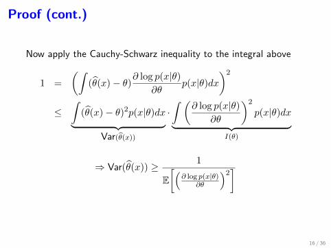
Proof (cont.)

Now apply the Cauchy-Schwarz inequality to the integral above

1 =

(∫(θ(x)− θ)∂ log p(x|θ)

∂θp(x|θ)dx

)2

≤∫

(θ(x)− θ)2p(x|θ)dx︸︷︷︸Var(θ(x))

·∫ (


)2

p(x|θ)dx︸︷︷︸I(θ)

⇒ Var(θ(x)) ≥ 1

E[(


)2]

16 / 36

Fisher information matrixUnder the regularity condition that

E[∂ log p(x|θ)

∂θ

]= 0 ∀ θ,

the Fisher Information Matrix is

I(θ∗) := E

[(∂

∂θlog p(x|θ)

)(∂

∂θlog p(x|θ)

)> ∣∣∣θ=θ∗

]

≡ −E[

∂2

∂θ∂θ>log p(x|θ)

∣∣∣θ=θ∗

]∈ Rp×p.

so that

[I(θ∗)]j,k ≡ −E[∂2 log p(x|θ)∂θj∂θk

∣∣∣θ=θ∗

]Note that if θ∗ ∈ R (i.e. p = 1), then

I(θ∗) := E

[(∂ log p(x|θ)

∂θ

)2 ∣∣∣θ=θ∗

]= −E

[∂2 log p(x|θ)

∂θ2

∣∣∣θ=θ∗

].

19 / 36

The CRLB is not always attained.

Example: Phase Estimation (Kay p 33)

xn = A cos(2πf0n+ φ) + wn, n = 1, · · · , N

The amplitude and frequency are assumed known, and we want toestimate the phase φ. We assume

wn ∼ N (0, σ2)iid.

p(x|φ) =1

(2πσ2)N/2exp

{− 1

2σ2

N∑n=1

(xn −A cos(2πf0n+ φ))2

}

20 / 36

Example: (cont.)

∂ log p(x|φ)

∂φ=− A

σ2

N∑n=1

(xn sin(2πf0n+ φ)

−A2

sin(4πf0n+ 2φ)

)∂2 log p(x|φ)

∂φ2=− A

σ2

N∑n=1

(xn cos(2πf0n+ φ)

−A2

cos(4πf0n+ 2φ)

)−E[∂2 log p(x|φ)

∂φ2

]=A

σ2

N∑n=1

(A cos2(2πf0n+ φ)− A

2cos(4πf0n+ 2φ)

)

=A2

σ2

N∑n=1

(1/2 + 1/2 cos(4πf0n+ 2φ)

− cos(4πf0n+ 2φ))

21 / 36

Example: (cont.)

Since 1N

∑cos(4πf0n) ≈ 0 for f0 not near 0 or 1/2,

I(φ) ≈ NA2

2σ2

Var(φ) ≥ 2σ2

NA2

In this case, it can be shown that there does not exist a g such that

∂ log p(x|φ)

∂φ= I(φ)(g(x)− φ)

Therefore an unbiased phase estimator that attains the CRLB doesnot exist. However, a MVUE estimator may still exist – only itsvariance will be larger than the CRLB. Sufficient statistics can helpus determine whether a MVUE still exists.

22 / 36

CRLB For Signals in White Gaussian Noise

(Kay p 35)

xn = sn(θ) + wn, n = 1, · · · , N

p(x|θ) =1

(2πσ2)N/2exp

{− 1

2σ2

N∑n=1

(xn − sn(θ))2

}∂ log p(x|θ)

∂θ=

1

σ2

N∑n=1

(xn − sn(θ))∂sn(θ)

∂θ

∂2log p(x|θ)∂θ2

=1

σ2

N∑n=1

[(xn − sn(θ))

∂2sn(θ)

∂θ2−(∂sn(θ)

∂θ

)2]

E[∂2log p(x|θ)

∂θ2

]= − 1

σ2

N∑n=1

(∂sn(θ)

∂θ

)2

23 / 36

CRLB For Signals in WGN, cont.

Var(θ) ≥ σ2∑Nn=1

(∂sn(θ)∂θ

)2Signals that change rapidly as θ changes result in more accurateestimators.

24 / 36

Definition: Efficient estimator

An estimator which is unbiased and attains the CRLB is said to beefficient.

Example:

Sample-mean estimator is efficient.

Example: Efficient estimators are MVUE, but MVUE may notbe efficient.

Suppose three unbiased estimators exist for a parameter θ.

Efficient and MVUE MVUE but not efficient

25 / 36

CRLBs for Subspace Models

We saw before that we could compute a minimum varianceunbiased estimator (MVUE) for θ in the subspace model

x = Hθ + w

by using sufficient statistics and the Rao-Blackwell Theorem.

Does this estimator achieve the Cramer-Rao Lower Bound?

26 / 36

Linear models

General Form of Linear Model (LM)

x = Hθ + w

x = observation vectorH = known matrix (“observation” or “system” matrix)θ = unknown parameter vectorw = vector of white Gaussian noise w ∼ N (0, σ2I)Probability Model for LM

x = Hθ + w

x ∼ p(x|θ) = N (Hθ, σ2I)

27 / 36

The CRLB and MVUE EstimatorRecall

θ = g(x)

achieves the CRLB if and only if


= I(θ)(g(x)− θ)

In the case of the linear model,


= − 1

2σ2∂

∂θ

[x>x− 2x>Hθ + θ>H>Hθ

]Now using identities

∂b>θ

∂θ= b and

∂θ>Aθ

∂θ= 2Aθ for A symmetric

we have∂ log p(x|θ)

∂θ=

1

σ2[H>x−H>Hθ].

28 / 36

Now

I(θ) =E

[(∂

∂θlog p(x|θ)

)(∂

∂θlog p(x|θ)

)>]=

1

σ4E[H>(x−Hθ)(x−Hθ>)H

]=

1

σ4H>E

[(x−Hθ)(x−Hθ>)

]H

=H>H

σ2

Assuming H>H is invertible, we can write


=H>H

σ2︸︷︷︸I(θ)

(H>H)−1H>x︸︷︷︸θ(x)

−θ

θ = (H>H)−1H>x is MVUE Estimator for x = Hθ + w

29 / 36

Theorem: MVUE Estimator for the LM

If the observed data can be modeled as

x = Hθ + w

where w ∼ N (0, σ2I) and H>H is invertible, then the MVUEestimator is

θ = (H>H)−1H>x = H#x,

the covariance of θ is

Cθ

= σ2(H>H)−1

and θ attains the CRLB. Note:

θ ∼ N (θ, σ2(H>H)−1)

30 / 36

Linear Model Examples

Example: Curve fitting.

x(tn) = θ1 + θ2tn + · · ·+ θptp−1n + w(tn), n = 1, · · · , N

w(tn)iid∼ N (0, σ2)

x = [x(t), · · · , x(tn)]>

θ = [θ1, θ2, · · · , θp]>

H =

1 t1 · · · tp−11

1 t2...

......

1 tN tp−1N

← Vandermode Matrix

The MVUE estimator for θ is

θ = (H>H)−1H>x

31 / 36

Example: System Identification.

There is an FIR filter h, and we want to know its impulse response.To estimate this, we send a probe signal u through the filter andobserve

x[n] =

m−1∑k=0

h[k]u[n− k] + w[n], n = 0, · · · , N − 1.

Goal: given x and u estimate h. In matrix form

x =

u[0] 0 · · · 0u[1] u[0] · · · 0

......

...u[N − 1] u[N − 2] · · · u[N −m]

︸︷︷︸

H

h[0]

...

h[m− 1]

︸︷︷︸

θ

+w

θ = (H>H)−1H>x← MVUE estimator

Cov(θ) = σ2(H>H)−1 = Cθ

32 / 36

Example: (cont.)

An important question in system id is how to chose the input u[n]to “probe” the system most efficiently. First note that

Var(θi) = e>i Cθei

where ei = [0, · · · , 0, 1, 0, · · · , 0]>. Also, since C−1θ

is symmetricand positive definite, we can factor it using Cholesky factorization:

C−1θ

= D>D,

where D is invertible. Note that

(e>i D>(D>)−1ei)

2 = 1

33 / 36

Example: (cont.)

The Schwarz inequality shows

1 = (e>i D>(D>)−1ei)

2

= 〈Dei, (D>)−1ei〉

≤ (e>i D>Dei)(e

>i

((D>)−1

)>(D>)−1ei) (1)

= (e>i D>Dei)(e

>i (D>D)−1ei)

= (e>i C−1θei)(e

>i Cθei)

⇒ Var(θi) ≥1

(e>i C−1θei)

=σ2

[H>H]ii

The minimum variance is achieved when equality is attained abovein (1).

34 / 36

Example: (cont.)

This happens only if ξ1 = Dei is proportional to ξ2 = (D>)−1ei.That is ξ1 = cξ2for some constant c. Equivalently

D>Dei = ciei for i = 1, 2, · · · ,m

D>D = C−1θ

=H>H

σ2

D>Dei =H>H

σ2ei = ciei

Combining these equations in matrix form

H>H = σ2

c1 0 0

0. . . 0

0 0 cm

.∴ In order to minimize the variance of the MVUE estimator, u[n]should be chosen to make H>H diagonal.

35 / 36

When the CRLB Doesn’t Help

The Cramer-Rao lower bound gives a necessary and sufficientconditionfor the existence of an efficient estimator. However,MVUEs are not necessarily efficient. What can we do in suchcases?

The Rao-Blackwell theorem, when applied in conjunction with acomplete sufficient statistic, gives another way to find MVUEs thatapplies even when the CRLB is not defined.

36 / 36

11. Cramer Rao Bounds

Documents

Transcript of 11. Cramer Rao Bounds