Computational Game Theory Spring Semester, 2011/2012

Lecture 1: March 7Lecturer: Amos Fiat Scribe: Eran Nir and Yael Amsterdamer

1.1 Computational Game Theory

1.1.1 Agenda

The course will cover the following material:

• Introduction to Game Theory

• Examples

• Matrix form Games

• Utility

• Solution concepts

• Dominant Strategies

• Nash Equilibria

• Complexity

• Mechanism Design: reverse game theory

1.1.2 CGT in Computer Science

The study of Game Theory in the context of Computer Science exists only inthe last 15 years. The purpose is to understand problems from the perspectiveof computability and algorithm design. Computing involves many differentselfish entities, and therefore involves game theory. An example to this is theinternet:

• Many players (end-users, ISVs, Infrastructure Providers).

1

2 Lecture 1: March 7

• Players wish to maximize their own benefit and act accordingly.

• The trick is to design a system where its beneficial for the player tofollow the rules.

The interest in game theory is divided into theory studying and industry use:

Theory:

• Algorithm design

• Complexity

• Quality of game states (Equilibrium states in particular)

• Study of dynamics

Industry:

• Sponsored search

• Other auctions

1.1.3 Game Theory

Some explication in a nutshell:

• Rational Player: Prioritizes possible actions according to utility or cost,and strives to maximize utility or to minimize cost.

• Competitive Environment: More than one player at the same time.

Game Theory analyzes how rational players behave in competitive environ-ments.

1.2. THE PRISONER’S DILEMMA 3

1.2 The Prisoner’s Dilemma

The prisoner’s dilemma is the most known example of a game in which twoindividuals might not cooperate, even if it appears that it is in their bestinterest to do so.

The dilemma is as follows: two men are arrested upon committing acrime, but the police don’t have enough evidence for conviction. The twoare held in separate rooms for interrogation, and offered the same deal bythe police: If one of them confesses and testifies against his partner, thebetrayer receives 2 years in jail, while the one who kept silent receives a 6years sentence. if both keep silent, both are sentenced to 3 years in jail (forother charges). if both cooperate with the police, both receive 5 years. Thetable representation of the game is as follows, where for each pair (x, y), x isthe utility of the row player, and y is the utility of the column player:

Keep silent DefectKeep silent (3,3) (6,2)

Defect (2,6) (5,5)

Since the game is played only once (the situation in the police station isassumed not to return on itself), each player is only concerned with gettingless jail time. Regardless of what the other prisoner chooses to do - keep silentor betray - one will benefit more by betraying. The symmetry of the gamemeans both prisoners will betray, therefore receiving the highest possibletotal jail time of all options (10 total years), while cooperating and keepingsilent would’ve ended with the lowest possible jail time (6).

In such case, where no matter what the other players in the game do, oneprefers a specific action, we call this action a ”dominant strategy”. In thisgame, betraying is the dominant strategy.

1.3 ISP Routing

Another variation of the Prisoner’s Dilemma is the ISP (Internet ServiceProviders) Routing Game. ISPs often share their physical networks for free,and so in some cases an ISP can either choose to route traffic in its ownnetwork or via a partner network. the routing choice made by the originatingISP also affects the load at the destination ISP.

4 Lecture 1: March 7

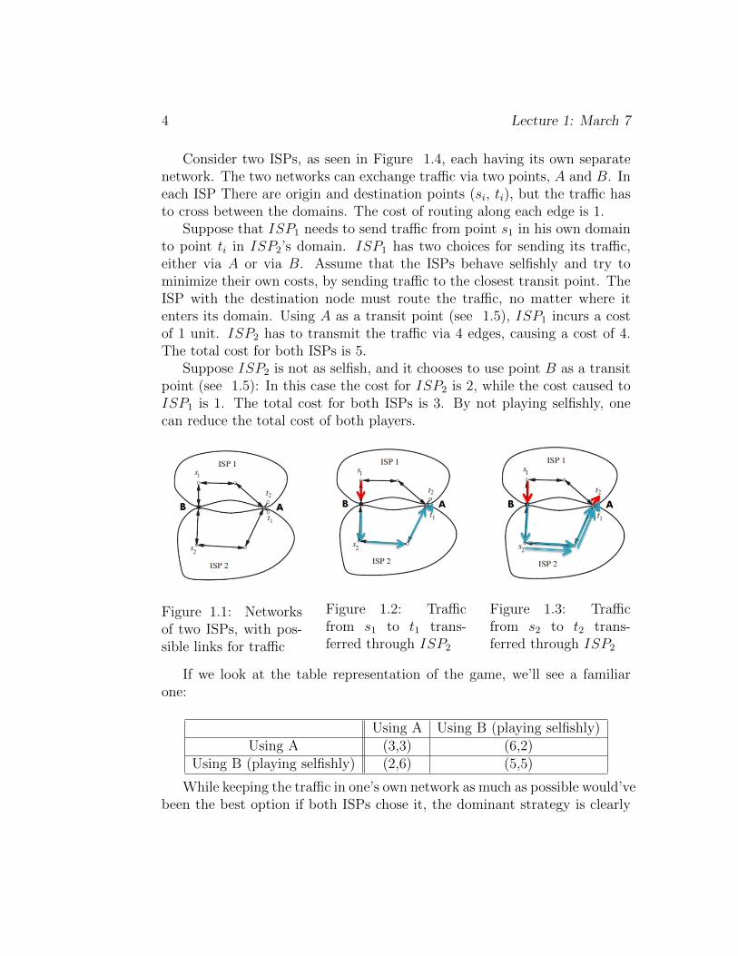
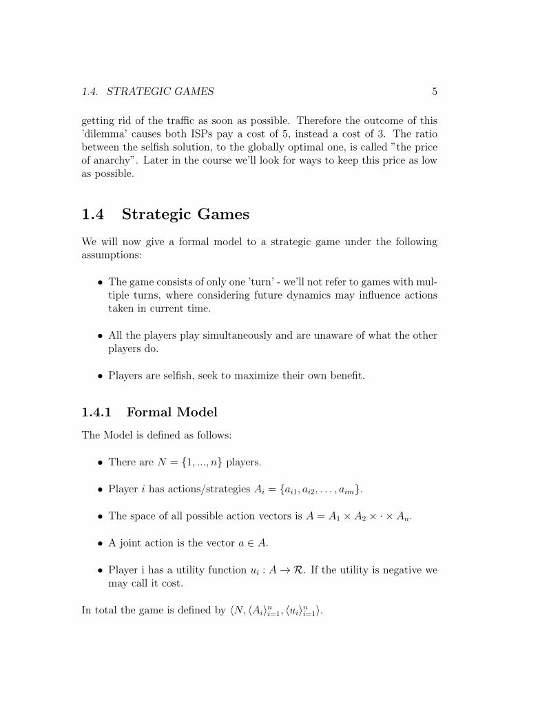
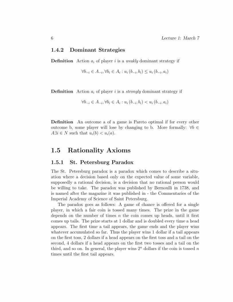
Consider two ISPs, as seen in Figure 1.4, each having its own separatenetwork. The two networks can exchange traffic via two points, A and B. Ineach ISP There are origin and destination points (si, ti), but the traffic hasto cross between the domains. The cost of routing along each edge is 1.

Suppose that ISP1 needs to send traffic from point s1 in his own domainto point ti in ISP2’s domain. ISP1 has two choices for sending its traffic,either via A or via B. Assume that the ISPs behave selfishly and try tominimize their own costs, by sending traffic to the closest transit point. TheISP with the destination node must route the traffic, no matter where itenters its domain. Using A as a transit point (see 1.5), ISP1 incurs a costof 1 unit. ISP2 has to transmit the traffic via 4 edges, causing a cost of 4.The total cost for both ISPs is 5.

Suppose ISP2 is not as selfish, and it chooses to use point B as a transitpoint (see 1.5): In this case the cost for ISP2 is 2, while the cost caused toISP1 is 1. The total cost for both ISPs is 3. By not playing selfishly, onecan reduce the total cost of both players.

Figure 1.1: Networksof two ISPs, with pos-sible links for traffic

Figure 1.2: Trafficfrom s1 to t1 trans-ferred through ISP2

Figure 1.3: Trafficfrom s2 to t2 trans-ferred through ISP2

If we look at the table representation of the game, we’ll see a familiarone:

Using A Using B (playing selfishly)Using A (3,3) (6,2)

Using B (playing selfishly) (2,6) (5,5)

While keeping the traffic in one’s own network as much as possible would’vebeen the best option if both ISPs chose it, the dominant strategy is clearly

1.4. STRATEGIC GAMES 5

getting rid of the traffic as soon as possible. Therefore the outcome of this’dilemma’ causes both ISPs pay a cost of 5, instead a cost of 3. The ratiobetween the selfish solution, to the globally optimal one, is called ”the priceof anarchy”. Later in the course we’ll look for ways to keep this price as lowas possible.

1.4 Strategic Games

We will now give a formal model to a strategic game under the followingassumptions:

• The game consists of only one ’turn’ - we’ll not refer to games with mul-tiple turns, where considering future dynamics may influence actionstaken in current time.

• All the players play simultaneously and are unaware of what the otherplayers do.

• Players are selfish, seek to maximize their own benefit.

1.4.1 Formal Model

The Model is defined as follows:

• There are N = {1, ..., n} players.

• Player i has actions/strategies Ai = {ai1, ai2, . . . , aim}.

• The space of all possible action vectors is A = A1 × A2 × · × An.

• A joint action is the vector a ∈ A.

• Player i has a utility function ui : A→ R. If the utility is negative wemay call it cost.

In total the game is defined by 〈N, 〈Ai〉ni=1, 〈ui〉ni=1〉.

6 Lecture 1: March 7

1.4.2 Dominant Strategies

Definition Action ai of player i is a weakly dominant strategy if

∀b−i ∈ A−i,∀bi ∈ Ai : ui (b−i, bi) ≤ ui (b−i, ai)

Definition Action ai of player i is a strongly dominant strategy if

∀b−i ∈ A−i,∀bi ∈ Ai : ui (b−i, bi) < ui (b−i, ai)

Definition An outcome a of a game is Pareto optimal if for every otheroutcome b, some player will lose by changing to b. More formally: ∀b ∈A∃i ∈ N such that ui(b) < ui(a).

1.5 Rationality Axioms

1.5.1 St. Petersburg Paradox

The St. Petersburg paradox is a paradox which comes to describe a situ-ation where a decision based only on the expected value of some variable,supposedly a rational decision, is a decision that no rational person wouldbe willing to take. The paradox was published by Bernoulli in 1738, andis named after the magazine it was published in - the Commentaries of theImperial Academy of Science of Saint Petersburg.

The paradox goes as follows: A game of chance is offered for a singleplayer, in which a fair coin is tossed many times. The prize in the gamedepends on the number of times n the coin comes up heads, until it firstcomes up tails. The prize starts at 1 dollar and is doubled every time a headappears. The first time a tail appears, the game ends and the player winswhatever accumulated so far. Thus the player wins 1 dollar if a tail appearson the first toss, 2 dollars if a head appears on the first toss and a tail on thesecond, 4 dollars if a head appears on the first two tosses and a tail on thethird, and so on. In general, the player wins 2n dollars if the coin is tossed ntimes until the first tail appears.

Rationality Axioms 7

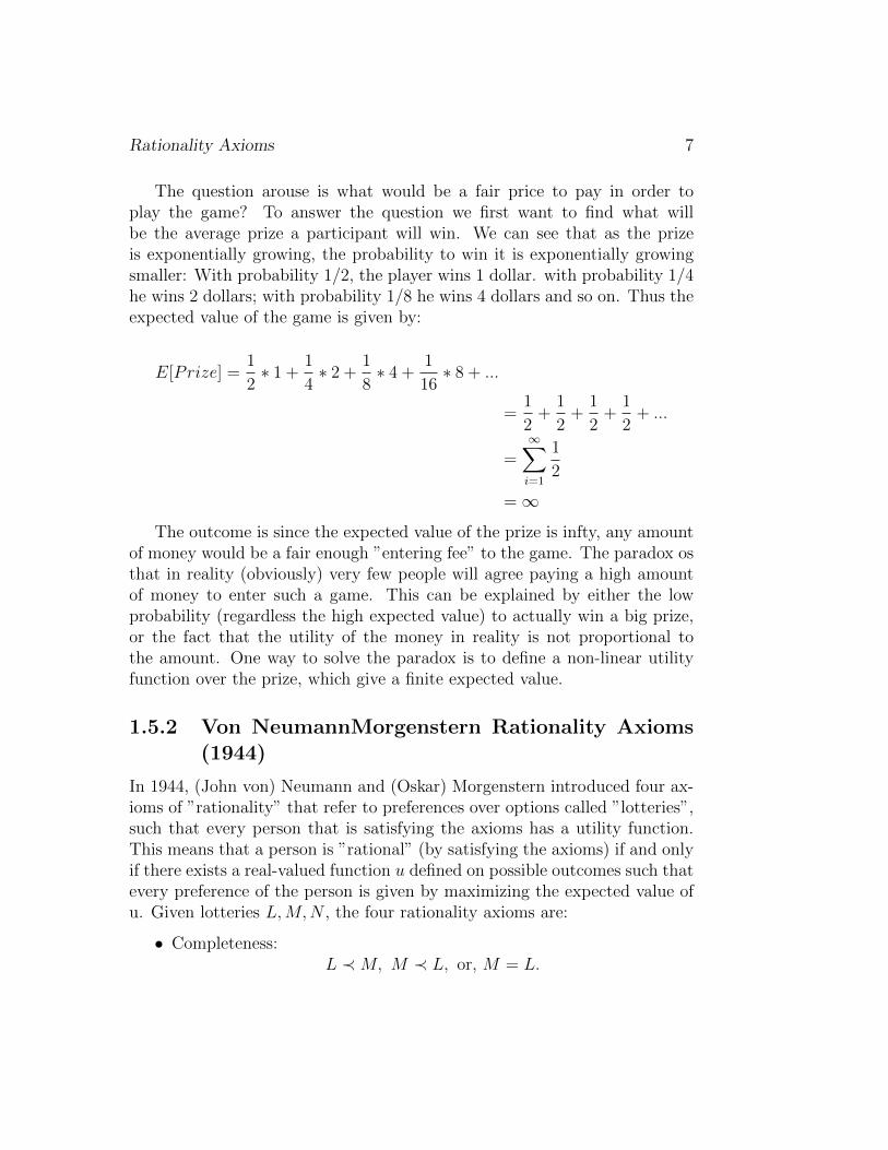
The question arouse is what would be a fair price to pay in order toplay the game? To answer the question we first want to find what willbe the average prize a participant will win. We can see that as the prizeis exponentially growing, the probability to win it is exponentially growingsmaller: With probability 1/2, the player wins 1 dollar. with probability 1/4he wins 2 dollars; with probability 1/8 he wins 4 dollars and so on. Thus theexpected value of the game is given by:

E[Prize] =1

2∗ 1 +

1

4∗ 2 +

1

8∗ 4 +

1

16∗ 8 + ...

=1

2+

1

2+

1

2+

1

2+ ...

=∞∑i=1

1

2

=∞

The outcome is since the expected value of the prize is infty, any amountof money would be a fair enough ”entering fee” to the game. The paradox osthat in reality (obviously) very few people will agree paying a high amountof money to enter such a game. This can be explained by either the lowprobability (regardless the high expected value) to actually win a big prize,or the fact that the utility of the money in reality is not proportional tothe amount. One way to solve the paradox is to define a non-linear utilityfunction over the prize, which give a finite expected value.

1.5.2 Von NeumannMorgenstern Rationality Axioms(1944)

In 1944, (John von) Neumann and (Oskar) Morgenstern introduced four ax-ioms of ”rationality” that refer to preferences over options called ”lotteries”,such that every person that is satisfying the axioms has a utility function.This means that a person is ”rational” (by satisfying the axioms) if and onlyif there exists a real-valued function u defined on possible outcomes such thatevery preference of the person is given by maximizing the expected value ofu. Given lotteries L,M,N , the four rationality axioms are:

• Completeness:L ≺M, M ≺ L, or, M = L.

8 Lecture 1: March 7

• Transitivity:

if L �M � N, then L � N.

• Continuity:

if L �M � N then there exists p ∈ [0, 1] s.t. pL+ (1− p)N = M .

• Independence:

if L ≺M, then for any N and p ∈ (0, 1] : pL+(1−p)N ≺ pM+(1−p)N.

As written above, Von Neumann and Morgenstern proved that given thoseaxioms, we have a real-valued utility function over lotteries, and holds: giventwo lotteries, u(αL1 + (1− α)L2) = αu(L1) + (1− α)u(L2).

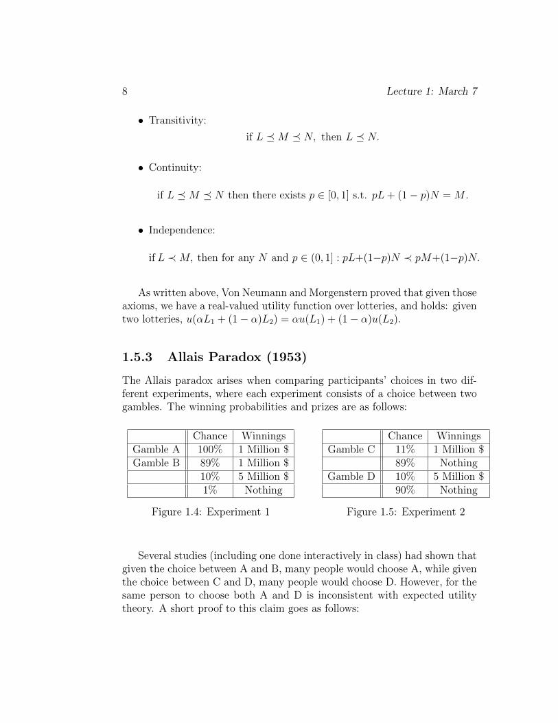
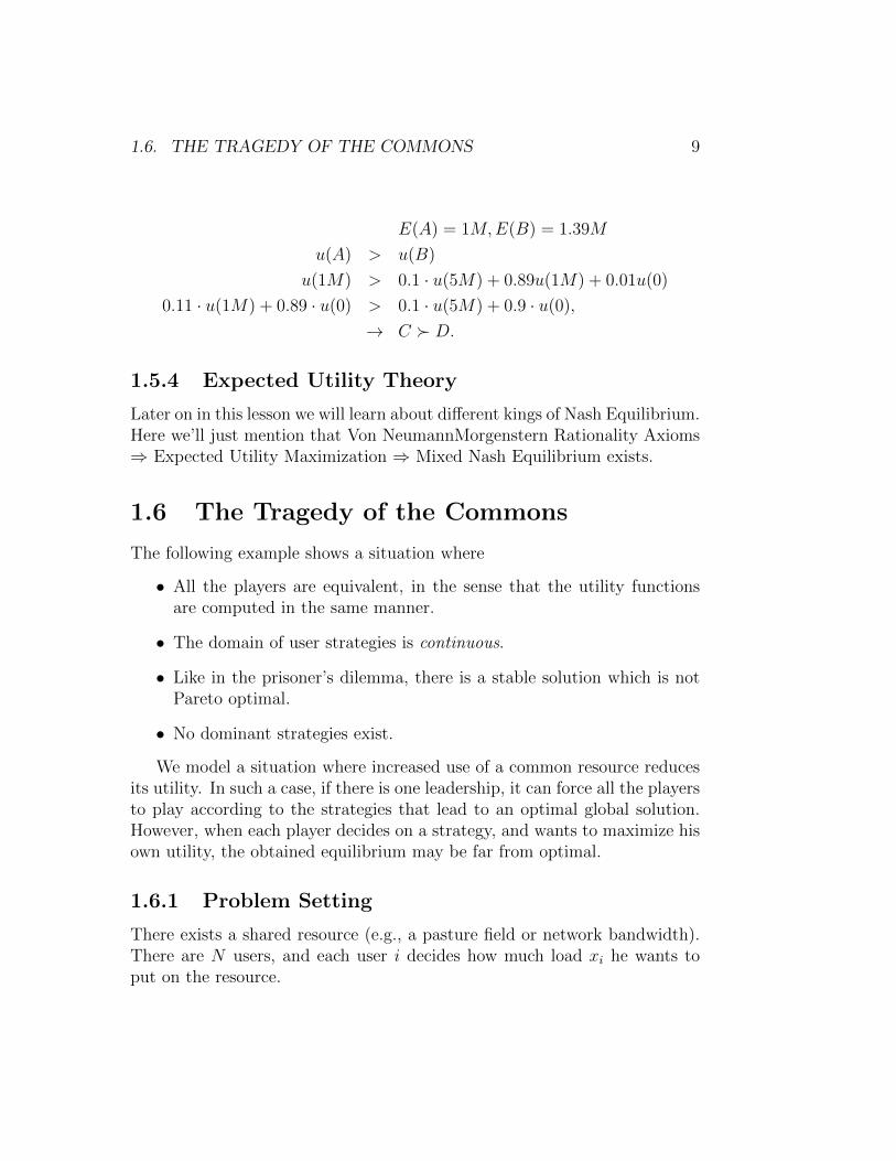
1.5.3 Allais Paradox (1953)

The Allais paradox arises when comparing participants’ choices in two dif-ferent experiments, where each experiment consists of a choice between twogambles. The winning probabilities and prizes are as follows:

Chance WinningsGamble A 100% 1 Million $Gamble B 89% 1 Million $

10% 5 Million $1% Nothing

Figure 1.4: Experiment 1

Chance WinningsGamble C 11% 1 Million $

89% NothingGamble D 10% 5 Million $

90% Nothing

Figure 1.5: Experiment 2

Several studies (including one done interactively in class) had shown thatgiven the choice between A and B, many people would choose A, while giventhe choice between C and D, many people would choose D. However, for thesame person to choose both A and D is inconsistent with expected utilitytheory. A short proof to this claim goes as follows:

1.6. THE TRAGEDY OF THE COMMONS 9

E(A) = 1M,E(B) = 1.39M

u(A) > u(B)

u(1M) > 0.1 · u(5M) + 0.89u(1M) + 0.01u(0)

0.11 · u(1M) + 0.89 · u(0) > 0.1 · u(5M) + 0.9 · u(0),

→ C � D.

1.5.4 Expected Utility Theory

Later on in this lesson we will learn about different kings of Nash Equilibrium.Here we’ll just mention that Von NeumannMorgenstern Rationality Axioms⇒ Expected Utility Maximization ⇒ Mixed Nash Equilibrium exists.

1.6 The Tragedy of the Commons

The following example shows a situation where

• All the players are equivalent, in the sense that the utility functionsare computed in the same manner.

• The domain of user strategies is continuous.

• Like in the prisoner’s dilemma, there is a stable solution which is notPareto optimal.

• No dominant strategies exist.

We model a situation where increased use of a common resource reducesits utility. In such a case, if there is one leadership, it can force all the playersto play according to the strategies that lead to an optimal global solution.However, when each player decides on a strategy, and wants to maximize hisown utility, the obtained equilibrium may be far from optimal.

1.6.1 Problem Setting

There exists a shared resource (e.g., a pasture field or network bandwidth).There are N users, and each user i decides how much load xi he wants toput on the resource.

10 Lecture 1: March 7

In a case when the sum of user loads∑N

i=1 xi is ≤ 1, the resource isoverloaded and for every user i the utility ui = 0. In any other case, the

utility of a user i is computed by the formula ui = xi

(1−

∑Nj=1 xj

). I.e.,

increasing the user load xi will not always increase the utility ui (because ofthe second factor, that decreases as the overall load increases). The optimalchoice of xi thus depends on the choices of the other uses.

1.6.2 The Rational Solution

If the choices of the other users are fixed (as unknown parameters) we cancompute the maximum point of the utility function for a single user, as fol-lows:ui = xi

(1−

∑Nj=1 xj

)= xi

(1− xi −

∑j 6=i xj

)– developing the utility for-

mula.

dui

dxi= −2xi +

(1−

∑j 6=i xj

)= 0 – deriving according to xi and

setting the derivative to 0.

⇔ 2xi = 1−∑

j 6=i xj

⇔ xi = 1− xi −∑

j 6=i xj = 1−∑N

j=1 xj – moving one xi to the right-hand size.

⇒∑N

j=1 xj = N −N∑N

j=1 xj – since all the players areequivalent.

⇔ (N + 1)∑N

j=1 xj = N

⇔∑N

j=1 xj = NN+1

– we got an expression for thesum of loads.

⇒ xi = 1−∑N

j=1 xj = 1− NN+1

= N+1−NN+1

= 1N+1

– using the expression in theformula for xi.

⇒ ui = xi

(1−

∑Nj=1 xj

)= 1

N+1· 1N+1

= 1(N+1)2

– the resulting utility.

Assuming that the players are rational, each of them must choose xi =

1.7. NASH EQUILIBRIUM 11

1N+1

and consequently get utility ui = 1(N+1)2

. Is this state Pareto optimal?

If every user i chose xi = 12N

instead, the utility of each user would be

ui = xi

(1−

N∑j=1

xj

)=

1

2N

(1−N · 1

2N

)=

1

2N

(1− 1

2

)=

1

2N· 1

2=

1

4N

. This utility is asymptotically larger than 1(N+1)2

. Every player would in-

crease his utility by moving from the rational solution ∀i xi = 1(N+1)2

to the

new solution, ∀i xi = 12N

. Thus, the rational solution is not Pareto optimal.Still, given the new solution, as our previous computation shows, every userwill have the motivation to change his choice, and increase his utility at theexpense of the others.

1.7 Nash Equilibrium

he obtained solution in the “tragedy of the commons” was not globally opti-mal due to the assumption that players are not collaborating with each other.Each player tries to maximize his own utility given the choices of the others.When no player can increase his utility alone (by changing his choice), we geta Nash equilibrium (named after John Nash, who first defined this situationin game theory). The formal definition:

Definition If xi, x−i are certain strategies of user i and the other usersrespectively, {xi, x−i} is called a Nash equilibrium if

∀1 ≤ i ≤ N,∀yi ∈ Ai : ui (xi, x−i) ≥ ui (yi, x−i)

According to this definition, we actually proved in the tragedy of thecommons that ∀1 ≤ i ≤ N : xi = 1

N+1is a Nash Equilibrium.

Definition Given the strategies of other players x−i, the best response of aplayer i is the set of all strategies that together with x−i maximize the utilityfor player i. It is denoted by

BRi(x−i) = arg maxxi

ui (xi, x−i)

12 Lecture 1: March 7

In a Nash equilibrium, every player’s strategy must be a best response,according to the definition above. We get an equivalent definition for Nashequilibrium.

Definition (An equivalent definition) For users 1, . . . , N , a set of choicesx1 . . . xN is a Nash equilibrium if

∀1 ≤ i ≤ N : xi ∈ BRi(x−i)

1.7.1 Battle of the Sexes

We next describe some examples for games where Nash equilibria exist. Inthe first example, “the battle of the sexes”, the situation is as follows: acouple tries to decide whether to go to the opera or to a sports game. Onepartner favors the sports game, and the other favors the opera, but in anycase they prefer to stay together. The following table expresses their utility,where the row player is the one who favors the sports game. Recall that ifa cell table contains a pari (x, y), x is the utility of the row player for thecombination of strategies, and y is the utility of the column player.

Sports OperaSports (4,3) (2,2)Opera (1,1) (3,4)

In this situation we have two Nash equilibria. For the strategy combi-nation {Sports, Sports} ∈ A, each of the players will lose by changing theirstrategy: if the row player switches to the Opera strategy, the gain of thisplayer will be reduced from 4 to 1; and if the column player switches to theopera, the utility of this player will be reduced to from 3 to 2. The strategycombination {Opera,Opera} ∈ A is also a Nash equilibrium from similarreasons.

Unlike the tragedy of the commons, here there is no clear strategy thata rational player should choose. We do not know how to achieve one ofthe possible Nash equilibria; we only know that if we initialize the players’strategies according to one of the equilibria, and the players are selfish and

1.8. MIXED STRATEGIES 13

not collaborating with each other, then none of them will have an incentiveto switch to a different strategy.

1.7.2 Routing Game

The second example for a Nash equilibrium is similar, only that here theplayers have an incentive to choose different strategies rather than the samestrategy. Consider two common routes that connect the users to the internet.Route A consists of only 1 link, on which the cost of a single packet is 1, andthe cost of 2 packets together is 3 per packet. Route B consists of 2 links,where the price of a single packet per link is 1, and the price of 2 packets is 2per packet per link. This is summarized in the following table (the row andcolumn players are symmetric).

A BA (3,3) (1,2)B (2,1) (4,4)

Here, (1,2) and (2,1) are Nash equilibrium states, since if either the rowplayer or the column player change their strategy alone, they will only in-crease their cost.

1.8 Mixed Strategies

1.8.1 Matching Pennies

Consider a situation, where two players have to choose heads or tails each.The row player wins a point if they make the same choice, and loses one ifthey choose differently. The column player, however, wins a point if theychoose differently, and loses a point if they choose the same. We get thefollowing utility table:

Heads TailsHeads (1,-1) (-1,1)Tails (-1,1) (1,-1)

14 Lecture 1: March 7

In each of the four states, one player wins and one loses. The loser alwayshas an incentive to change his strategy, and become a winner. Thus, in thisgame, no Nash equilibrium exists.

What can the players do in such a situation? Assume that the players areallowed not to choose a single strategy, but a distribution over the strategies.The row player will choose heads with probability p (and tails with probabil-ity 1− p, and similarly the column player will choose heads with probabilityq. We can now compute the expected utility of, e.g., the row player, for eachchoice he makes: if he chooses heads, he will win one point with probabil-ity q (the column player also chooses heads; we assume that the players areindependent). With probability 1 − q, the column player will choose tailsand the row player will lose one point. Thus the expected utility of the rowplayer for choosing heads is uheads = 1 · q+ (−1) · (1− q) = 2q− 1. Choosingtails is symmetric, thus the expected utility for the row player for choosingtails is utails = (−1) · q + 1 · (1− q) = 1− 2q.

The row player will choose a mixed strategy only if one or more strategieshave the maximum utility. In this case, this means that uheads = utails ⇔2q − 1 = 1− 2q ⇔ q = 1

2.

1.8.2 Strategy Distributions

If Ai is the domain of possible strategies for the player i, then ∆ (Ai) is thedomain of all possible probabilistic distributions over Ai. It can be viewedas the simplex of strategies, where each strategy has a probability between 0and 1, and the sum of probabilities is 1.

Definition For the player i, a mixed strategy is a choice of pi ∈ ∆ (Ai).

A single possible strategy (as opposed to a mixed strategy) is also calleda pure strategy.

Definition For players 1, . . . , N , a joint mixed strategy is a vector of mixedstrategies ~P = {p1, . . . , pN}. The outcome of the game is a joint mixedstrategy.

Definition A mixed Nash equilibrium is a joint mixed strategy where forevery player i, given the (mixed) strategies of the other players p−i, i cannotincrease his expected utility by changing his strategy. More formally,

∀i ∈ 1 . . . N,∀qi ∈ ∆ (Ai) : Exi∼pi,x−i∼p−i[ui (x1, . . . , xN)] ≥ Exi∼qi,x−i∼p−i

[ui (x1, . . . , xN)]

Mixed Strategies 15

(p−i is used to denote the joint distribution of all the players but i).

We will define two useful notations.

Definition The support of a mixed strategy pi is the set of all strategieswith non-zero probability in pi, denoted by

support(pi) = {ai | pi(ai) > 0}

Definition (In the mixed case) Given the mixed strategies of other playersp−i, the best response of a player i is the set of all pure strategies that togetherwith p−i give the maximal expected utility for player i. The best responseset is denoted by

BRi(p−i) = arg maxai

Ex−i∼p−i[ui (ai, x−i)]

For each mixed strategy, there exists a pure strategy with a greater orequal expected utility. To see that, recall that an expectation is alwayssmaller than the maximal case. Take a mixed strategy pi ∈ ∆ (Ai), and thejoint mixed strategy of the other players p−i. We can choose a pure strategyai ∈ support(pi), such that the expected utility of ai, p−i is maximal. I.e., thisis the “maximal case”, and the expected utility of pi, p−i is the “expectation”.Thus, the expected utility of ai, p−i has to be greater.

In a Nash equilibrium, we choose a positive probability only for strategiesai that maximize the utility with respect to the mixed strategies of the others.This actually means that

∀i : support(pi) ⊆ BRi(p−i)(an important property of mixed Nash equilibrium).

For such a mixed strategy there exist only pure strategies with equal expectedutility, and not strictly higher. We can use this property to formulate anequivalent definition of mixed Nash equilibrium.

Definition (Equivalent definition) A mixed Nash equilibrium is a joint mixedstrategy where for every player i, given the (mixed) strategies of the otherplayers p−i, i cannot increase his expected utility by changing his strategy toa (different) pure strategy. Formally,

∀i ∈ 1 . . . N,∀ai ∈ Ai : Exi∼pi,x−i∼p−i[ui (x1, . . . , xN)] ≥ Ex−i∼p−i

[ui (ai, x−i)]

16 Lecture 1: March 7

1.8.3 Rock Paper Scissors

The following utility table describes the results of the rock-paper-scissorsgame.

Rock Paper ScissorsRock (0,0) (-1,1) (1,-1)Paper (1,-1) (0,0) (-1,1)

Scissors (-1,1) (1,-1) (0,0)

Similarly to the matching Pennies game, here there exists no pure Nashequilibrium. However, there exists a mixed one: 1

3probability for each strat-

egy for each of the players. If we fix this strategy for the column player,than the expected utility for each choice of the row player is 0. This meansthat any of the choices is a best response and can be in the support of themixed strategy of the row player. To achieve an equilibrium (i.e., to allowall strategies to be best responses also for the column player), we should giveequal probability to each of the row player choices.

1.8.4 Nash Theorem

Theorem 1.1 (Nash, 1951) Any game with a finite set of players and afinite set of strategies has a mixed Nash equilibrium.

We will show an algorithm for finding the mixed Nash equilibrium, in agame with two players. The following is the matrix of utilities: (r11, c11) · · · (r1n, c1n)

.... . .

...(rm1, cm1) · · · (rmn, cmn)

We will also define two sets of variables, p(1), . . . , p(m) for the proba-

bilities assigned to each of the strategies of the row player, and similarlyq(1), . . . , q(n), for the column player. We showed that in a mixed Nashequilibrium, support(p) ⊆ BRrow(q). This means that the expected utility ofevery strategy of the row player should be the same, and this works in a sym-metrical way for the column player. Assume that the support of the mixedstrategies of the players are fixed. If I = {i1, . . . , ik} are the indices of the

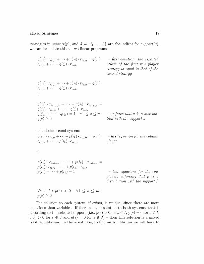
Mixed Strategies 17

strategies in support(p), and J = {j1, . . . , jl} are the indices for support(q),we can formulate this as two linear programs:

q(j1) · ri1,j1 + · · ·+ q(jl) · ri1,jl = q(j1) ·ri2,j1 + · · ·+ q(jl) · ri2,jl

– first equation: the expectedutility of the first row playerstrategy is equal to that of thesecond strategy

q(j1) · ri2,j1 + · · ·+ q(jl) · ri2,jl = q(j1) ·ri3,j1 + · · ·+ q(jl) · ri3,jl...

q(j1) · rik−1,j1 + · · · + q(jl) · rik−1,jl =q(j1) · rik,j1 + · · ·+ q(jl) · rik,jlq(j1) + · · · + q(jl) = 1 ∀1 ≤ s ≤ n :q(s) ≥ 0

– enforce that q is a distribu-tion with the support J

... and the second system:

p(i1) · ci1,j1 + · · ·+ p(ik) · cik,j1 = p(i1) ·ci1,j2 + · · ·+ p(ik) · cik,j2

– first equation for the columnplayer

...

p(i1) · ci1,jl−1+ · · · + p(ik) · cik,jl−1

=p(i1) · ci1,jl + · · ·+ p(ik) · cik,jlp(i1) + · · ·+ p(ik) = 1 – last equations for the row

player, enforcing that p is adistribution with the support I

∀s ∈ I : p(s) > 0 ∀1 ≤ s ≤ m :p(s) ≥ 0

The solution to each system, if exists, is unique, since there are moreequations than variables. If there exists a solution to both systems, that isaccording to the selected support (i.e., p(s) > 0 for s ∈ I, p(s) = 0 for s 6∈ I,q(s) > 0 for s ∈ J and q(s) = 0 for s 6∈ J) – then this solution is a mixedNash equilibrium. In the worst case, to find an equilibrium we will have to

18 Lecture 1: March 7

try this for every possible support for p and q, a total of (2m − 1) (2n − 1)combinations (the −1 is there since the supports cannot be empty).

1.9 Location / Lemonade Stand Game

In this example, computing the Nash equilibria is not simple. There aremany veriations to this general problem, where N ice cream/lemonade ven-dors are choosing a location in a defined space. The utility of each vendoris determined by the distance between him, the neighbor vendors and thedefined space boundaries.

First variation The vendors are spread on the segment [0, 1]. The utilityof each vendor is half of the distance between him and his neighbors, i.e., ifthe location of the vendor i is xi, the utility of the vendor i is ui = xi+1−xi−1

2.

When N = 2, there is a pure Nash equilibrium with the two vendors as closeas possible to the middle point 1

2. When N = 3, no pure Nash equilibrium

exists.

Second variation If the vendors are spread on a circle instead of a seg-ment, there always exists a Nash equilibrium, with the vendors spread ateven distances from each other.

Links for other variations of the game and related competitions:

• http://martin.zinkevich.org/lemonade/

• http://tech.groups.yahoo.com/group/lemonadegame/