109. Grain price analysis in Ghana - AgEcon Searchageconsearch.umn.edu/bitstream/96165/2/109. Grain...
22
Grain price adjustment asymmetry: the case of cowpea in Ghana By Langyintuo, Augustine S. Contributed Paper presented at the Joint 3 rd African Association of Agricultural Economists (AAAE) and 48 th Agricultural Economists Association of South Africa (AEASA) Conference, Cape Town, South Africa, September 19-23, 2010.
-
Upload
nguyencong -
Category
Documents
-
view
217 -
download
0
Transcript of 109. Grain price analysis in Ghana - AgEcon Searchageconsearch.umn.edu/bitstream/96165/2/109. Grain...

Grain price adjustment asymmetry: the case of cowpea in Ghana
By
Langyintuo, Augustine S.
Contributed Paper presented at the Joint 3rd African Association of Agricultural
Economists (AAAE) and 48th Agricultural Economists Association of South Africa
(AEASA) Conference, Cape Town, South Africa, September 19-23, 2010.

0
Grain price adjustment asymmetry: the case of cowpea in Ghana
Augustine S. Langyintuo* Alliance for a Green Revolution in Africa (AGRA), Eden Square, Block 1, 5th Floor P O Box 66773, 00800 Westlands, Nairobi, KENYA
* Corresponding author: Dr. Augustine S. Langyintuo Tel: + 254 20 3675 309 Fax: + 254 20 3675 269 E-mail: [email protected]

1
Grain price adjustment asymmetry: the case of cowpea in Ghana
Abstract
Patterns in price adjustment in response to information are important to market
practitioners. This study looks at cowpea real wholesale price adjustment patterns in
Bolgatanga, Wa, Makola and Techiman markets in Ghana. Using Techiman as the central
market, a threshold autoregressive test for asymmetric price adjustment rejected the null
hypothesis of symmetric adjustment for only the Bolgatanga-Techiman price series. An
autoregressive conditional heteroskedastic regression indicates that wholesalers in
Bolgatanga market respond differentially to price signals from Techiman than those in the
other two markets. This suggests that policies targeting cowpea traders must recognize the
differential responses by wholesalers to information.
Keywords: Africa, Ghana, wholesalers, market information, autoregressive conditional
heteroskedasticity, threshold autoregressive
JEL Classification: D82, D43

2
Grain price adjustment asymmetry: the case of cowpea in Ghana
Introduction
Market regulators and those involved in marketing are interested in knowing the
response of local market prices to movement of prices in a central market. For instance, is
price volatility the same (symmetric) with upward versus downward movements or is it
greater or smaller (asymmetric)? If markets are perfectly competitive, prices adjust
symmetrically. On the other hand, asymmetric price adjustment can result with
oligopolistic behavior of middlemen, or inventory changes (Maccini, 1978; Blinder, 1982),
or level of market concentration and interventionist attitude of governments (Scherer &
Ross, 1990; Roberts, Stockton & Struckmeyer, 1994). Irrespective of the adjustment
process, theory suggests that at a given level, market price adjustment patterns would be
similar at various markets because of structural similarities. For example, wholesalers
throughout a region may react to price changes in the same way and retailers may react in a
different way.
Previous price adjustment studies on maize in Ghana (Alderman & Shively, 1996;
Alderman, 1993; Shively, 1996; Bidane & Shively, 1998; Abdulai, 2000) indicated that
wholesalers had similar price adjustment patterns throughout the country. Possibly, this is
because Ghana is self-sufficient in maize production and hence pricing decisions are
internal. In contrast, Ghana is not self-sufficient in cowpea production and has to import
mainly from Burkina Faso and Niger, through the informal sector, to satisfy domestic
demand (Langyintuo, et al., 2003). Initial point of entry is Bolgatanga in the Upper East
region (Map 1) where wholesalers take delivery of the grains. This means that cowpea
pricing policies in Burkina Faso and Niger probably have the greatest influence in that

3
region than in any other region. One would expect differences in price adjustments among
wholesalers or retailers in the Upper East region and those in the rest of the country
because of differences in their market information management processes.
This study looks at price adjustment patterns in the cowpea market in Ghana. It is
hypothesized that at the wholesale level price adjustment patterns are similar throughout
the country. Threshold autoregressive tests are used to examine this hypothesis. The extent
to which traders respond to information is examined using autoregressive conditional
heteroskedastic regression analysis. It is hoped that the results will contribute to the
growing literature on grain price adjustment patterns in developing economies.
Commodity markets integration and price adjustment processes
Two commodity markets are said to be spatially integrated if, when trade takes
place between them, price in the importing market equals price in the exporting market
plus the transportation and other transfer costs of moving the product between the two
markets (Tomek & Robinson, 1990). The most widely used approach to assessing the
short- and long-run integration of commodity markets is cointegration and error correction
model (Alexander & Wyeth, 1994; Alderman, 1993; Dercon, 1995; Abdulai, 2000; Kuiper
et al., 2003). The approach measures whether two markets are integrated in the long term
by assessing whether their prices wander within a fixed band. The usual two-step
residual-based test, due to Engle and Granger (1987), assumes perfect competition and
hence symmetric price adjustment. The Engle and Granger relationship that defines the
relationship between the price in a given local market ltP and the price in the central
market ctP at time t is given by:

4
tc
tl
t PaP 10 … (1)
where t is a random error term with constant variance that can be contemporaneously
correlated. If t , the marketing margin, is stationary in the test for market integration, then
long-run market integration can be said to prevail between the series, that is cointegrated
(Dwyer & Wallace, 1992). Short-run market integration tests, on the other hand, aim to
establish whether prices in different markets respond immediately to this long-run
relationship (Alexander & Wyth, 1994). The errors from the above equation are
differenced and regressed on the lag values as in equation (2) below to obtain .
ttt 1 … (2)
where t is white noise. Rejection of the null hypothesis of no cointegration indicates that
the residuals are stationary with mean zero (Engle and Granger, 1987).
To account for possible asymmetric adjustments as a result of imperfect
competition, the model developed by Enders and Granger (1998), which builds on
equations (1) and (2), can be employed. Enders and Granger (1998) observed that the
standard procedure to estimate in (2) serves as an attractor whereby its pull is strictly
proportional to the absolute value of t . The change in t is a product of and 1t ,
irrespective of whether 1t assumes a positive or negative sign implicitly assuming
symmetric adjustments. To account for asymmetric adjustments, Enders and Granger
(1998) therefore let the deviations from the long-run equilibrium in equation (2) behave as
a Threshold Autoregressive (TAR) process as:
5
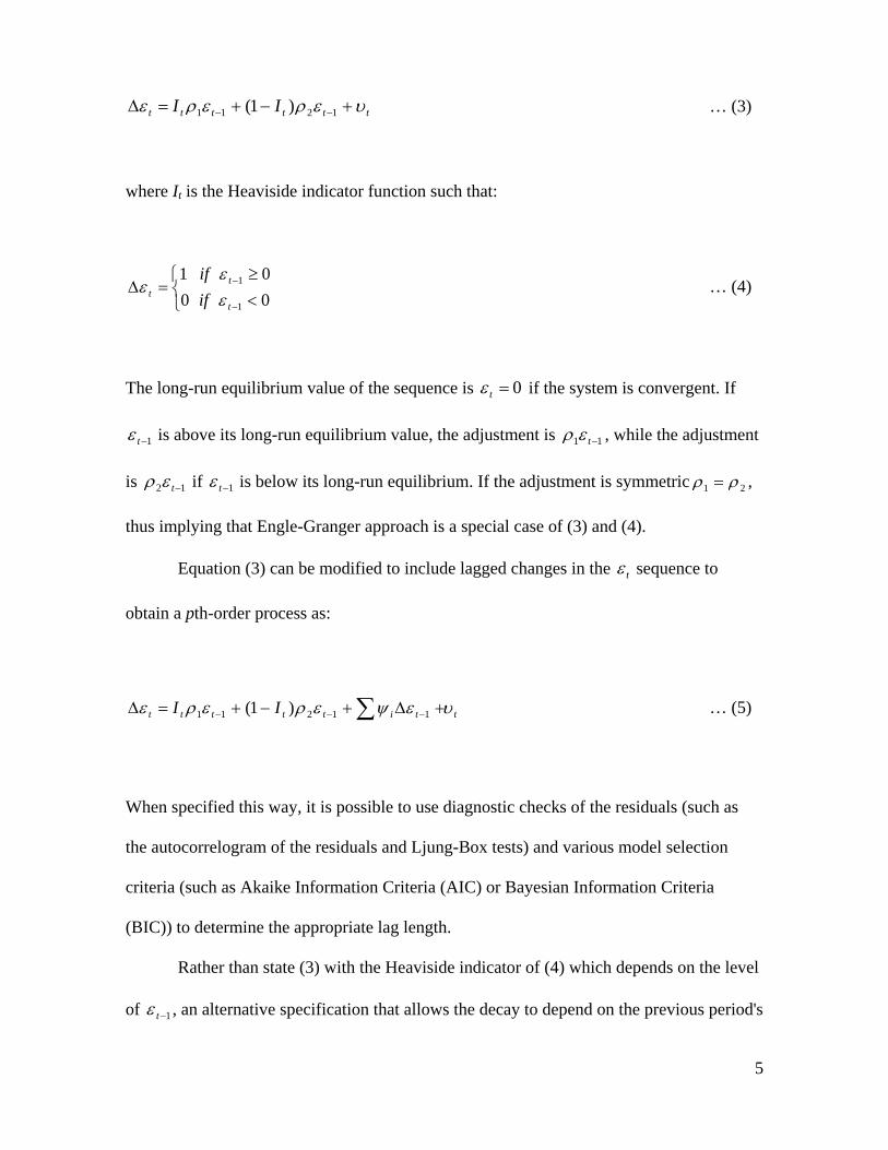
tttttt II 1211 )1( … (3)
where It is the Heaviside indicator function such that:
00
01
1
1
t
tt if
if
… (4)
The long-run equilibrium value of the sequence is 0t if the system is convergent. If
1t is above its long-run equilibrium value, the adjustment is 11 t , while the adjustment
is 12 t if 1t is below its long-run equilibrium. If the adjustment is symmetric 21 ,
thus implying that Engle-Granger approach is a special case of (3) and (4).
Equation (3) can be modified to include lagged changes in the t sequence to
obtain a pth-order process as:
ttittttt II 11211 )1( … (5)
When specified this way, it is possible to use diagnostic checks of the residuals (such as
the autocorrelogram of the residuals and Ljung-Box tests) and various model selection
criteria (such as Akaike Information Criteria (AIC) or Bayesian Information Criteria
(BIC)) to determine the appropriate lag length.
Rather than state (3) with the Heaviside indicator of (4) which depends on the level
of 1t , an alternative specification that allows the decay to depend on the previous period's

6
change in 1t is possible. One may thus consider the Heaviside indicator according to the
following rule:
00
01
1
1
t
tt if
ifI
… (6)
The choice of (3) and (6) is particularly useful when adjustment is asymmetric to the
degree that the series exhibits more "momentum" in one direction than the other (Enders
and Granger, 1998). Such models termed momentum-threshold autoregression (M-TAR)
models, exhibit little decay for positive values of 1 t but substantial decay for negative
values of 1 t if 21 . This implies that increases tend to persist but decreases tend
to revert quickly toward the attractor. The F-statistics for the null hypothesis using the
TAR and the M-TAR specifications are known, respectively, as and * . Their
distributions are determined by the number of lags in the augmented equation (5), the
number of variables and the type of deterministic elements included in the cointegrating
relationship. Appropriate critical values are tabulated in Enders and Granger (1998).
Sources of the data
Data for the analysis were monthly cowpea wholesale prices between July 1998
and June 2009 from Techiman, Makola (in Accra), Bolgatanga and Wa markets in the
Brong Ahafo, Greater Accra , Upper East and Upper West regions of Ghana, respectively
obtained from the Policy Planning, Monitoring and Evaluation Division (PPMED) of the
Ghana Ministry of Food and Agriculture (PPMED, 2009), deflated by the consumer price
index (CPI). In Ghana, the Techiman market may be regarded as the national grain market

7
where grains are aggregated and distributed to all parts of the country. Consequently, in
this study as in previous grain price integration studies in Ghana (Alderman & Shively,
1996; Alderman, 1993; Shively, 1996; Bidane & Shively, 1998; Abdulai, 2000), the
Techiman market was used as the central markt.
Cowpeas are produced mainly in the Northern, Upper East and Upper West regions
of Ghana sufficient to meet only 42% of the national demand (PPMED, 2009; Langyintuo,
et al., 2003). Grains are sold to merchants in the Techiman market soon after harvest where
part is distributed and part stored for resale later in the year to all consuming regions
(including the producing ones who later become consuming regions). Additional grains are
imported from Niger and Burkina Faso (Langyintuo, et al., 2003) using Bolgatanga as the
main import-point market where grains are sometimes re-packaged and then shipped to
Techiman for distribution. This means that traders in Bolgatanga also depend directly on
Niger and Burkina Faso for their cowpea supply after the domestic supplies are exhausted.
Small quantities of grains from Burkina Faso also enter the Ghanaian markets via the Wa
market.
Figure 1 shows that the real prices trend exhibit a gradual decline over time. The
Makola market consistently experienced the highest pieces but no consistency in the
market showing the lowest prices. It is unclear why prices in Bolgatanga were abnormally
low between October 2006 to December 2007.
Order of integration of cowpea wholesale price series in Ghana
A test for unit roots on the data series (Sargan & Bhargava, 1983; Dickey & Fuller,
1979, 1981) failed to reject the null hypothesis of unit root and test on the residuals
confirmed that the series are integrated to the order one, I(1) (Table 1). Table 2 shows that

8
the Engle-Granger test rejected the null hypothesis of no cointegration at the 1% level for
Bolgatanga and Wa, and 5% level for Makola. The implications of the the values of 0 for
Makola, Bolgatanga and Wa are that the absolute price margins linking the Techiman
central market and the local markets of Bolgatanga, Wa and Makola are respectively
¢0.47/kg, ¢0.30/kg and ¢0.56/kg.
Empirical results of cowpea price adjustment
Following the rejection of the null hypothesis of no cointegration the data were
tested for asymmetric adjustment using specifications (3), (4), and (6). Estimates of the
TAR results by equations (3) and (4) are presented in the top portion of Table 3. Various
lagged forms were estimated but the AIC and BIC both chose one lagged form. Comparing
the estimated of 23.10, 14.43 and 14.51 for Techiman-Wa, Techiman-Makola, and
Tehiman-Bolgatanga respectively, with the critical values of 4.64 and 6.57 at the 5% and
1% levels, respectively, (Enders and Granger 1998), the null hypothesis of 021
can be rejected, confirming that prices are cointegrated.
The estimated 1 and 2 which give the rate of adjustment in prices towards
equilibrium given positive and negative deviations, respectively, are -0.27 and -0.43 for the
Techiman-Wa series. This suggests that approximately 27% of a positive deviation from
the long-run relationship between the two price series is eliminated within a month while
for a negative deviation, it is about 43%. Corresponding percentage deviations for the
Techiman- Makola series are 33% and 59%, respectively. Tests for asymmetric adjustment
(last column of Table 3) failed to reject the null hypothesis of 21 in both pairs
implying that neither price movement is stickier than the other. The estimates of 1 and

9
2 for the Techiman-Bolgatanga series are -0.15 and -0.41 implying that for a positive
deviation from the long-run relationship between the two price series, 15% is eliminated
within a month but for a negative deviation, the adjustment is 45%. The test for
asymmetric adjustment rejected the null hypothesis of symmetric adjustment ( 21 ) in
favor of asymmetric adjustments processes of the Bolgatanga market prices series to
changes in Techiman market prices series. Positive deviations are stickier than negative
ones. This means that wholesale traders are more reluctant to reduce prices if they
experience a positive price shock than to increase prices for a negative price shock.
The possible reason for these results is the degree of freedom with which merchants
can manipulate their stocks. Since wholesale traders in Wa and Makola rely mostly on
Techiman for their cowpea supplies, any price change in Techiman market are transmitted
instantaneously to Wa and Makola. In contrast, price changes in Techiman are not
transmitted instantaneously to Bolgatanga market because the latter is an import-point
market for cowpea from Niger and Burkina Faso meant for the Ghanaian markets.
Consequently any price changes in Techiman take time to filter to Niger and Burkina Faso
and back. When price increases in Techiman, traders in Bolgatanga are happy to exploit
the relatively lower prices in Niger and Burkina Faso until they adjust to the new price
levels. For a price decrease in Techiman, traders in Bolgatanga have shorter periods of
adjustment because by the time Niger and Burkina Faso start to experience the decrease,
Techiman prices would have re-adjusted and so will those in Bolgatanga.
For the Techiman-Bolgatanga market price series, M-TAR were estimated because
they followed asymmetric price adjustments. The values for the M-TAR model
presented in the second portion of Table 3 reject the null hypothesis that 021 ,

10
similar to the TAR results. The test for symmetric adjustment, that is, 21 , however,
could not be rejected suggesting that the observed asymmetry does not exhibit more
momentum in one direction than the other.
Price variability at the market level
An autoregressive conditional heteroskedastic regression (ARCH) model was
specified and estimated as in equation (1) to test the hypothesis that the local price
volatility is invariant to price changes. The estimated residuals from (1) were squared and
regressed on their lagged values and the lagged values of the local and central market
prices. A Lagrange multiplier test for ARCH(l) errors failed to reject the null hypothesis
of homoskedasticity at the 5% level in the variance for all the markets.
The estimated results presented in Table 4 indicate that with the Wa and Makola
series, an increase in local market prices reduce local price variability while an increase in
Techiman market price increases price variability in the local markets. The results suggest
that when there is an increase in the local market price relative to Techiman (the source),
traders tend to reduce inventories locally to exploit the higher price in the local markets
and re-stock from Techiman where price is relatively lower. This thus reduces price
volatility locally. On the other hand, when price in Techiman increases relative to the local
price, traders are reluctant to sell grains procured from Techiman at a higher price on the
local market where the price is lower. They, therefore increase their inventories thus
triggering higher local prices and hence higher price volatility.
In contrast, Table 4 indicates that variability in Bolgatanga market price increases
when previous local market price increases but decreases when previous market price in
the Techiman market increases. This suggests that when local price increases relative to

11
central market price, traders increase stocks in anticipation for higher prices in subsequent
markets. When they take delivery of the grains from Niger and Burkina Faso, they are
reluctant to supply to the Techiman market but rather increase their inventories in
Bolgatanga. This results in the higher volatility locally. On the other hand, when the
Techiman market price increases, traders reduce inventories to exploit the higher price
thereby reducing local price volatility. These results thus confirm the differential response
to market signals among wholesalers.
Summary and conclusions
A threshold autoregressive (TAR) model was used to test the hypothesis that at the
wholesale level in Ghana, cowpea price adjustment patterns are similar throughout the
country. The model employs monthly cowpea wholesale prices deflated by the CPI
between July 1998 and June 2009 from Techiman, Makola (in Accra), Bolgatanga and Wa
markets, respectively. With Techiman as central market, the series were observed to be
cointegrated.
The TAR test for asymmetric adjustment failed to reject the null hypothesis of
symmetric adjustment for the Techiman-Wa and Techiman-Makola series but rejected the
null hypothesis of equal adjustment for theTechiman-Bolgatanga series in favor of
asymmetric adjustment. In the latter case, only 15% of any increase is eliminated within a
month compared with 41% for a decrease, implying that price increases are stickier than
decreases. The differential price adjustment between Bolgatanga on one hand and Wa and
Makola on the other was confirmed by the autoregressive conditional heteroskedastic
regression model results. Whereas variability in Bolgatanga market prices increase when

12
previous local market prices increase but decrease when previous market price in the
Techiman (central) market increase, the opposite is true for the other markets.
The above results failed to support the initial hypothesis that wholesalers respond
to information similarly. The fact that wholesalers at the import-point market, directly
involved in the importation and distribution of cowpea, respond differently to information
compared with all others contradict the symmetric behavior of maize wholesalers observed
by Abdulai (2000). The relatively greater impacts of foreign grain pricing policies on
cowpea compared with maize wholesalers might be a factor for these results. This
asymmetric information from foreign policies is possibly greatest in the import-point
markets than all other parts of the country, hence the differential response of traders to
market information. This means that any market policy targeting wholesalers in similar
informal grain markets must recognize the differential response of wholesalers to
information to ensure the desired impacts.

13
References
Abdulai, A., 2000. Spatial price transmission and asymmetry in Ghanaian maize market.
Journal of Development Economics. 63 (3) 327-349.
Alderman, H., 1993. Intercommodity price transmittal: analysis of markets in Ghana.
Oxford Bulletin of Economics and Statistics 55 (1), 43-64.
Alderman, H., Shively, G., 1996. Economic reform and food prices: evidence from
markets in Ghana. World Development 24 (3), 521-534.
Alexander, C., Wyeth, J., 1994. Cointegration and market integration: an application to the
Indonesian rice market. Journal of Development Studies 30 (2), 303-328.
Badiane, O., Shively, G.E., 1998. Spatial integration, transport costs, and the response of
local prices to policy changes in Ghana. Journal of Development Economics 56 (2),
411-431.
Blinder, A.S., 1982. Inventories and sticky prices: more on microfoundations of
macroeconomics. American Economic Review 72 (3), 365-400.
Dercon, S., 1995. On market integration and liberalization: method and application to
Ethiopia. Journal of Development Studies 32 (1), 112-143.
Dwyer, G.P., Wallace, M.S., 1992. Cointegration and market efficiency. Journal of
International Money and Finance 11 (4), 318-327.
Enders, W., Granger, C.W.J., 1998. Unit-root tests and asymmetric adjustment with an
example using the term structure of interest rates. Journal of Business and
Economic Statistics 16 (3), 304-311.
Enders, W., Siklos, P.L., 1998. The term structure: testing for an equilibrium with
asymmetric adjustment, Mimeo. Iowa State University Working Paper.

14
Engle, R.F., Granger, C.W.J., 1987. Cointegration and error correction: representation,
estimation and testing. Econometrica 55 (2), 251-280.
Kuipera, W. E, Lutz, C. van Tilburg, A., 2003. Vertical price leadership on local maize
markets in Benin. Journal of Development Economics, (71) , 417-433.
Langyintuo, A. S., Lowenberg-DeBoer, J., Faye, M., Lambert, D., Ibro, G., Moussa, B.,
Kergna, A., Kushwaha, S., Musa, S., Ntoukam, G., 2003. Cowpea Supply and
Demand in West and Central Africa. Field Crops Research. 82 (2-3), 215-231.
Maccini, L.J., 1978. The impact of demand and price expectations on the behavior of
prices. American Economic Review 68 (1), 134-145.
PPMED (Policy Planning, Monitoring and Evaluation Division). 2009. Estimates of
production of selected crops in Ghana. Ministry of Agriculture, Accra, Ghana.
Roberts, J.M., Stockton, D.J., Struckmeyer, C.S., 1994. Evidence on the flexibility of
prices. Review of Economics and Statistics 76 (1), 142-150.
Scherer, F.M., Ross, D., 1990. Industrial Market Structure and Economic Performance. 3rd
Edn. Houghton Mifflin, Boston.
Shively, G.E., 1996. Food price variability and economic reform: an ARCH Approach for
Ghana. American Journal of Agricultural Economics 78 (1), 126-136.
Tomek, W. G., Robinson, K., L., 1990. Agricultural Product prices, Third Edition. Cornell
Inuversity Press, Ithaca.

15
Table 1: Test of order of integration on individual series with constant and trend
Market
T-Test
0*
-Test
0* 0*
Bolgatanga -3.0935 3.3471 4.7848
Wa -2.3096 2.4320 3.0391
Makola -2.6513 2.6807 3.5293
Techiman -3.1251 3.5632 5.2065
Critical values (10%) -3.130 4.030 5.340
Note: The general form of the equation run was:
n
j tjtjtt PPtP11
* . Where 1* . Reject the null
hypothesis of unit root if the t-test statistic is smaller than the critical value.

16
Table 2: Engle –Granger cointegration results ( tC
tL
t PP 10 ; TechimanP c ) (n =
132)
Market 0 1
Adjusted
R-square AIC1
BIC2
Engle-
Granger test3
(1 = 0)
Bolgatanga
0.466
(0.27)
0.853
(9.23)
85.23 0.39 445.39 456.92 -5.009
Wa
0.304
(2.90)
0.645
(11.37)
129.27 0.49
316.64
328.17 -3.985
Makola
0.560
(4.22)
0.926
(15.05)
226.43 0.63
338.12
349.65 -3.750
Note: In parenthesis are the t-ratios
1 AIC (Akaike Information Criterion) is calculated as: n*log(SSR) + 2*k [where n =
number of observations; SSR = sum of squared residuals; k = number of
regressors].
2 BIC (Baysian Information Criterion) BIC is calculated as: n*log(SSR) + k*log(n)
[where n = number of observations; SSR = sum of squared residuals; k = number of
regressors].
3 Critical values of the Engle-Granger test for no cointegration are -3.5 and -3.95 for
the 5% and 1% levels, respectively.

17
Table 3: Results of the symmetric and asymmetric adjustment in cowpea prices
Market 1
2 AIC BIC a
21
Threshold Autoregressive (TAR) model
Wa
-0.267
(-2.709)
-0.428
(-4.639)
238.29
244.04
14.430
1.419
(0.236)
Makola
-0.330
(-2.742)
-0.593
(-6.219)
288.00
293.75
23.098
2.940
(0.088)
Bolgatanga
-0.146
(-2.094)
-0.411
(-4.963)
307.54
313.30
14.510
6.030
(0.015)
Momentum Threshold Autoregressive (M-TAR) model
Bolgatanga
-0.145
(-1.309)
-0.382
(-3.405)
321.26
327.05
6.654
2.261
(0.132)
Notes: Figures in parenthesis in columns 2 and 3 are the t-statistics for the null hypotheses:
01 and 02 , but in column 6 they are significant levels for the
corresponding F statistics of the null hypothesis that the adjustment coefficients are
equal.
aSample values for the test statistics of the TAR and M-TAR are, respectively
and * . [Critical values of are 4.99, 5.98 and 8.21 for the 10, 5 and 1%,
respectively. Those for * are respectively 5.43, 6.45 and 8.75; (Enders and
Siklos, 1998)].

18
Table 4: The ARCH model results
0 2
1t ltP 1 c
tP 1 F-
statistic
Techiman - Wa 0.0215
(0.526)
0.3766
(4.469)
-0.0044
(-2.835)
0.0360
(4.227)
10.272
Techiman - Makola
0.0748
(1.063)
0.2508
(2.333)
-0.0004
(-3.006)
0.0028
(2.041)
2.878
Techiman - Bolgatanga 0.0162
(0.214)
0.6840
(12.720)
0.1706
(3.889)
-0.1694
(-3.038)
93.415
Note: In parenthesis are the t-statistics

19
Figure 1: Real cowpea price series in selected markets in Ghana

20
Map1: Map of Ghana showing locations of study markets
Locations of study markets


![Shadowrun: Street Grimoire, 2nd Printing · HEALTH SPELLS 109 Ambidexterity 109 Alleviate Addiction 109 Alleviate [Allergy] 109 Awaken 109 ... Advanced Alchemy/ Ritual/Spellcasting](https://static.fdocuments.in/doc/165x107/5f0367d57e708231d4090d07/shadowrun-street-grimoire-2nd-printing-health-spells-109-ambidexterity-109-alleviate.jpg)