1.05 Theory and Observations – Forward Modeling/Synthetic Body … · 1.05 Theory and...

1.05 Theory and Observations – Forward Modeling/SyntheticBody Wave SeismogramsV. F. Cormier, University of Connecticut, Storrs, CT, USA

ª 2007 Elsevier B.V. All rights reserved.

1.05.1 Introduction 157

1.05.2 Plane-Wave Modeling 159

1.05.2.1 Elastic Velocities and Polarizations 159

1.05.2.2 Superposition of Plane Waves 161

1.05.3 Structural Effects 161

1.05.3.1 Common Structural Effects on Waveforms 161

1.05.3.2 Deep-Earth Structural Problems 164

1.05.4 Modeling Algorithms and Codes 165

1.05.4.1 Reflectivity 166

1.05.4.2 Generalized Ray 168

1.05.4.3 WKBJ-Maslov 168

1.05.4.4 Full-Wave Theory and Integration in Complex p Plane 170

1.05.4.5 DRT and Gaussian Beams 171

1.05.4.6 Modal Methods 172

1.05.4.7 Numerical Methods 173

1.05.5 Parametrization of the Earth Model 176

1.05.5.1 Homogeneous Layers Separated by Curved or Tilted Boundaries 176

1.05.5.2 Vertically Inhomogeneous Layers 177

1.05.5.3 General 3-D Models 177

1.05.6 Instrument and Source 178

1.05.6.1 Instrument Responses and Deconvolution 179

1.05.6.2 Far-Field Source Time Function 179

1.05.7 Extensions 181

1.05.7.1 Adapting 1-D Codes to 2-D and 3-D 181

1.05.7.2 Hybrid Methods 181

1.05.7.3 Frequency-Dependent Ray Theory 181

1.05.7.4 Attenuation 182

1.05.7.5 Anisotropy 183

1.05.7.6 Scattering 184

1.05.8 Conclusions 185

References 185

1.05.1 Introduction

Body waves are solutions of the elastic equation of

motion that propagate outward from a seismic sourcein expanding, quasi-spherical wave fronts, much like

the rings seen when a rock is thrown in a pond. The

normals to the wave fronts, called rays, are useful in the

illustrating body waves’ interactions with gradients and

discontinuities in elastic velocities and as well as their

sense of polarization of particle motion. Except for thespecial cases of grazing incidence to discontinuities,

body-wave solutions to the equations of motion are

nearly nondispersive. All frequencies propagate at

nearly the same phase and group velocities. Hencethe body wave excited by an impulsive, delta-like,

seismic source-time function will retain its delta-like

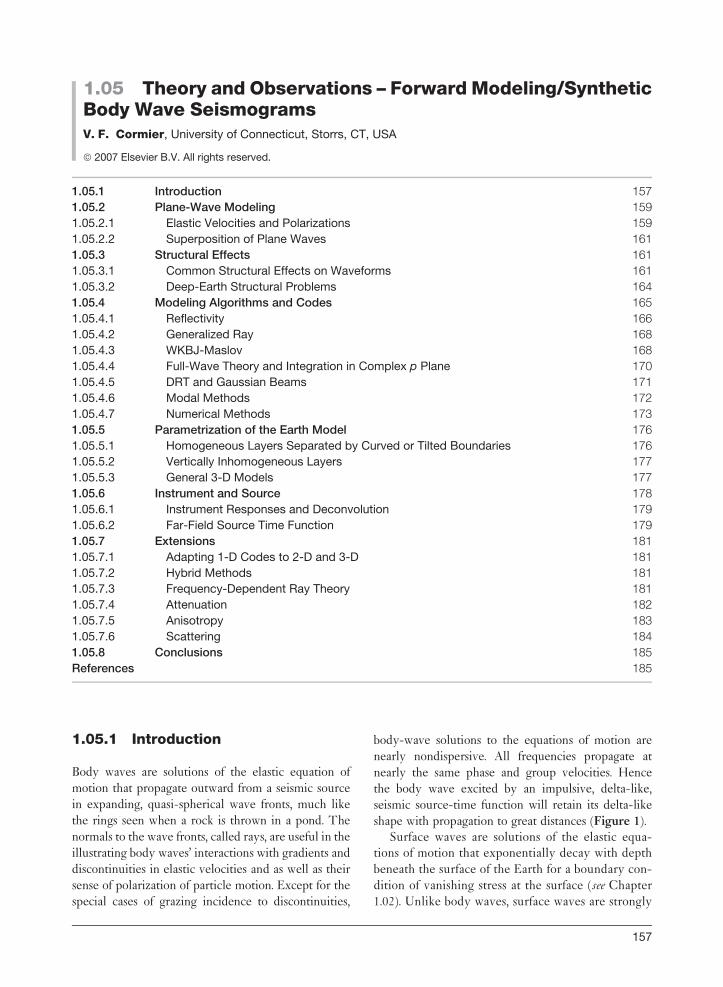
shape with propagation to great distances (Figure 1).Surface waves are solutions of the elastic equa-

tions of motion that exponentially decay with depth

beneath the surface of the Earth for a boundary con-

dition of vanishing stress at the surface (see Chapter1.02). Unlike body waves, surface waves are strongly

157

dispersed in the Earth, having phase and group velo-cities that depend on frequency. Observations ofsurface waves in the 0.001–0.1 Hz band of frequenciescan constrain structure of the crust and upper mantleof the Earth, but only body waves provide informa-tion on the elastic velocities of the deeper interior ofthe Earth, all the way to its center. Summing modesof free oscillation of the Earth can represent bothbody and surface waves. The most efficient represen-tation of the highest frequency content body waves,however, is given by propagating wave front or ray-type solutions of the elastic equations.

In a homogeneous Earth, the wave fronts of bodywaves are spherical, with radii equal to the distancefrom the source to an observation point on the wavefront. Since the density of kinetic energy at a pointin time is simply the surface area of the wave front,the particle velocity of a body wave is inverselyproportional to the distance to the source. Thisinverse scaling of amplitude with increasing distanceis termed the geometric spreading factor, R. Evenin an inhomogeneous Earth, the inverse-distancescaling of body-wave amplitude can be used tomake a rough estimate of the behavior of amplitudeversus distance.

Rays follow paths of least or extremal time, repre-senting a stationary phase approximation to a

solution of a wave equation, Fourier-transformed in

space and time. The least-time principle is expressed

by Snell’s law. In spherical geometry and radially

varying velocity, Snell’s law is equivalent to the con-

stancy of a ray parameter or horizontal slowness p.

The ray parameter is defined by p ¼ r sin(i )/v(r),

where i is the acute angle between the intersection

of a ray path and a surface of radius r, and v is the

body-wave velocity. Snell’s law is obeyed by ray

paths in regions of continuously varying velocity as

well as by the ray paths of reflected and transmitted/

converted waves excited at discontinuities. Since

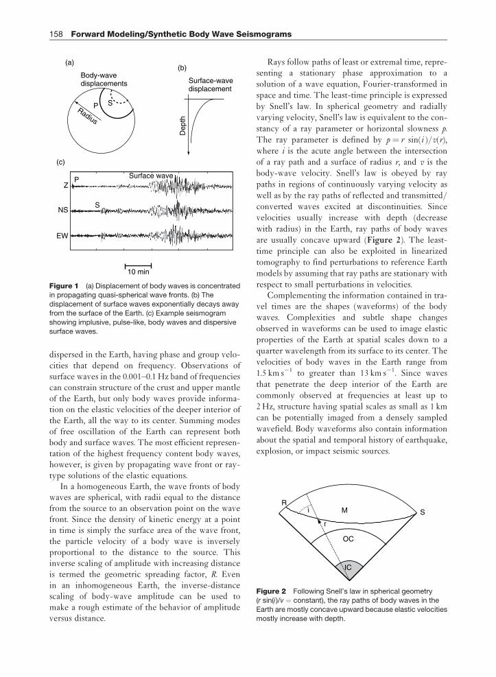
velocities usually increase with depth (decrease

with radius) in the Earth, ray paths of body waves

are usually concave upward (Figure 2). The least-

time principle can also be exploited in linearized

tomography to find perturbations to reference Earth

models by assuming that ray paths are stationary with

respect to small perturbations in velocities.Complementing the information contained in tra-

vel times are the shapes (waveforms) of the body

waves. Complexities and subtle shape changes

observed in waveforms can be used to image elastic

properties of the Earth at spatial scales down to a

quarter wavelength from its surface to its center. The

velocities of body waves in the Earth range from

1.5 km s�1 to greater than 13 km s�1. Since waves

that penetrate the deep interior of the Earth are

commonly observed at frequencies at least up to

2 Hz, structure having spatial scales as small as 1 km

can be potentially imaged from a densely sampled

wavefield. Body waveforms also contain information

about the spatial and temporal history of earthquake,

explosion, or impact seismic sources.

Surface-wavedisplacement

Dep

th

Body-wavedisplacements

Radius

Surface waveP

(c)

(a)(b)

Z

NS

EW

S

10 min

P S

Figure 1 (a) Displacement of body waves is concentratedin propagating quasi-spherical wave fronts. (b) The

displacement of surface waves exponentially decays away

from the surface of the Earth. (c) Example seismogram

showing implusive, pulse-like, body waves and dispersivesurface waves.

RM S

OC

i

r

IC

Figure 2 Following Snell’s law in spherical geometry(r sin(i )/v ¼ constant), the ray paths of body waves in the

Earth are mostly concave upward because elastic velocities

mostly increase with depth.

158 Forward Modeling/Synthetic Body Wave Seismograms

This chapter reviews algorithms for modeling theeffects of structure and source on teleseismic wave-forms (see Chapter 1.22). It will point to references forthe theoretical background of each algorithm andcurrently existing software. It will also make sugges-tions for the model parametrization appropriate toeach algorithm, and the treatment of source-timefunctions, instrument responses, attenuation, andscattering. Mathematical development of each algo-rithm can be found in textbooks in advanced andcomputational seismology (Dahlen and Tromp,1998; Aki and Richards, 1980, 2002; Kennett, 1983,2001; Cerveny, 2001; Chapman, 2004). A thoroughunderstanding of the derivation of each algorithmrequires a background that includes solution of par-tial differential equations by separation of variables,special functions, integral transforms, complex vari-ables and contour integration, and linear algebra.Practical use of each algorithm, however, oftenrequires no more than a background in simple calcu-lus and an intuitive understanding how a wavefieldcan be represented by superposing either wave frontsor modes at different frequencies.

1.05.2 Plane-Wave Modeling

1.05.2.1 Elastic Velocities andPolarizations

Two types of body waves were identified in earlyobservational seismology, P, or primary, for the firstarriving impulsive wave and S, or secondary, for asecond slower impulsive wave (Bullen and Bolt,1985). These are the elastic-wave types that propa-gate in an isotropic solid. In most regions of the Earth,elasticity can be well approximated by isotropy, inwhich only two elastic constants are required todescribe a stress–strain relation that is independentof the choice of the coordinate system. In the case ofanisotropy, additional elastic constants are requiredto describe the stress–strain relation. In a generalanisotropic solid, there are three possible body-wave types, P, and two quasi-S waves, each havinga different velocity.

The velocities of propagation and polarizations ofmotion of P and S waves can be derived from elasticequation of motion for an infinitesimal volume in acontinuum:

�q2ui

qt 2¼ þ�ij ; j ¼ – fi ½1�

where � is density, ui is the ith component of theparticle displacement vector U, �ij is the stress ten-sor, and fi is the ith component of body force thatexcites elastic motion. The elastic contact force in theith direction is represented by the jth spatial deriva-tive of the stress tensor, �ij ; j . The stress tensorelements are related to spatial derivatives of displa-cement components (strains) by Hooke’s law, whichfor general anisotropy takes the form

�ij ¼ cijkl uk; l ½2�

and for isotropy the form

�ij ¼ �qui

qxi

þ � qui

qxj

þ quj

qxi

� �½3�

where cijkl , �, and � are elastic constants. The sum-mation convention is assumed in [1]–[3], that is,quantities are summed over repeated indices.

Elastic-wave equations for P and S waves can bederived by respectively taking the divergence andcurl of the equation of motion [11], demonstratingthat volumetric strain, r?U , propagates with a

P-wave velocity,

VP ¼ffiffiffiffiffiffiffiffiffiffiffiffiffiffi�þ 2�

�

s¼

ffiffiffiffiffiffiffiffiffiffiffiffiffiffiffiffiffiffiffiK þ 4=3�

�

s½4a�

and rotational strain, r� U , propagates with theS-wave velocity,

VS ¼ffiffiffi�

�

r½4b�

Note that the P-wave velocity can be represented interms of either the Lame parameter � and shearmodulus � or the bulk modulus K and shear modulus�.

Alternatively, the phase velocities and polariza-tions of body waves can be derived by assumingpropagation of a plane wave having frequency !and a normal k of the form

Uðx; tÞ ¼ Aeði!t – k�xÞ ½5�

and substituting this form into [1]. This substitutionleads to an eigenvalue/eigenvector problem, inwhich the eigenvalues represent the magnitudes ofthe wavenumber vector k, and hence phase velocitiesfrom v ¼ !/jkj. The associated eigenvectors repre-sent the possible orientations of particle motion (e.g.,Keith and Crampin, 1977). For propagation in threedimensions (3-D), there are three possible eigenva-lues/eigenvectors, two of which are equal ordegenerate in an isotropic medium. The eigenvalue

Forward Modeling/Synthetic Body Wave Seismograms 159

with the fastest phase velocity is the P wave. It has aneigenvector or polarization that is in the direction ofthe P ray, normal to the wave front. In an isotropicmedium, the two degenerate eigenvalues and theireigenvectors are associated with the S wave. Theireigenvectors of polarization are perpendicular to theS ray, tangent to the wave front.

To facilitate the solution and understanding of theinteractions of the P- and S-wave types with discon-

tinuities in elastic moduli and/or density, it is

convenient to define a ray (sagittal) plane containing

the source, receiver, and center of the Earth. In an

isotropic medium, the S polarization, which depends

on the details of source excitation and receiver azi-

muth, is decomposed into an SV component, lying in

the sagittal plane, and an SH component, perpendi-

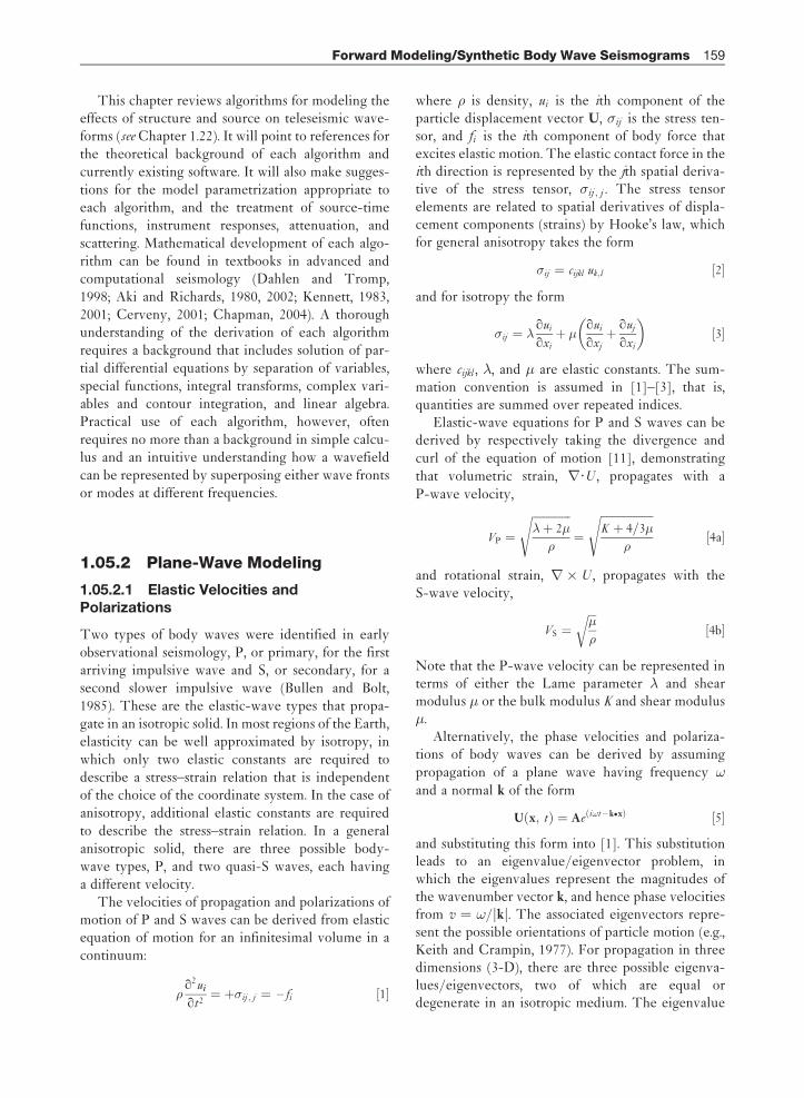
cular to the sagittal plane (Figure 3). At a

discontinuity in elastic velocity, SV waves can excite

converted–transmitted and reflected P waves and

vice versa, but SH waves can only excite transmitted

and reflected SH waves. The effects of body-

wave-type conversions on polarizations have con-

tributed to fundamental discoveries in deep Earth

structure. The most famous example of these discov-

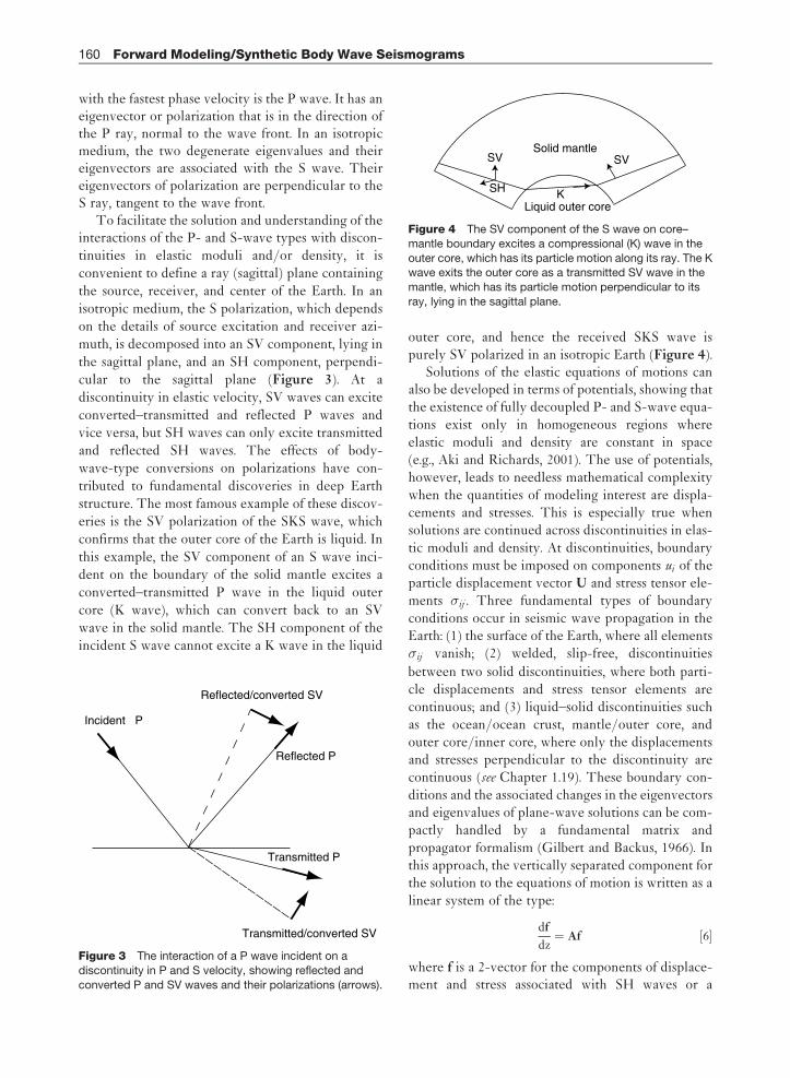
eries is the SV polarization of the SKS wave, which

confirms that the outer core of the Earth is liquid. In

this example, the SV component of an S wave inci-

dent on the boundary of the solid mantle excites a

converted–transmitted P wave in the liquid outer

core (K wave), which can convert back to an SV

wave in the solid mantle. The SH component of the

incident S wave cannot excite a K wave in the liquid

outer core, and hence the received SKS wave ispurely SV polarized in an isotropic Earth (Figure 4).

Solutions of the elastic equations of motions canalso be developed in terms of potentials, showing thatthe existence of fully decoupled P- and S-wave equa-tions exist only in homogeneous regions whereelastic moduli and density are constant in space(e.g., Aki and Richards, 2001). The use of potentials,however, leads to needless mathematical complexitywhen the quantities of modeling interest are displa-cements and stresses. This is especially true whensolutions are continued across discontinuities in elas-tic moduli and density. At discontinuities, boundaryconditions must be imposed on components ui of theparticle displacement vector U and stress tensor ele-ments �ij . Three fundamental types of boundaryconditions occur in seismic wave propagation in theEarth: (1) the surface of the Earth, where all elements�ij vanish; (2) welded, slip-free, discontinuities

between two solid discontinuities, where both parti-cle displacements and stress tensor elements arecontinuous; and (3) liquid–solid discontinuities suchas the ocean/ocean crust, mantle/outer core, andouter core/inner core, where only the displacementsand stresses perpendicular to the discontinuity arecontinuous (see Chapter 1.19). These boundary con-ditions and the associated changes in the eigenvectorsand eigenvalues of plane-wave solutions can be com-pactly handled by a fundamental matrix andpropagator formalism (Gilbert and Backus, 1966). Inthis approach, the vertically separated component forthe solution to the equations of motion is written as alinear system of the type:

df

dz¼ Af ½6�

where f is a 2-vector for the components of displace-ment and stress associated with SH waves or a

Solid mantleSVSV

SH KLiquid outer core

Figure 4 The SV component of the S wave on core–

mantle boundary excites a compressional (K) wave in the

outer core, which has its particle motion along its ray. The Kwave exits the outer core as a transmitted SV wave in the

mantle, which has its particle motion perpendicular to its

ray, lying in the sagittal plane.

Incident P

Reflected/converted SV

Reflected P

Transmitted P

Transmitted/converted SV

Figure 3 The interaction of a P wave incident on a

discontinuity in P and S velocity, showing reflected and

converted P and SV waves and their polarizations (arrows).


4-vector for the components of stress and displace-ment associated with P and SV waves; A is either a2� 2 matrix for SH waves or a 4� 4 matrix for P andSV waves; and derivative d/dz is with respect todepth or radius. The possibility of both up- anddown-going waves allows the most general solutionof the linear system in eqn [6] to be written as asolution for a fundamental matrix F, where the rowsof F are the components of displacement and stressand the columns correspond to up- and down-goingP and S waves. For P and SV waves, F is a 4� 4matrix; for SH waves, F is a 2� 2 matrix. An exampleof the fundamental matrix for SH waves in a homo-geneous layer is

F ¼ei!kzðz – zoÞ e – i!kzðz – zoÞ

ikz�ei!kzðz – zoÞ – ikz�e – i!kzðz – zoÞ

!½7�

where zo is the reference depth, and the sign of thecomplex phasors represents propagation with oragainst the z-axis to describe down- or up-goingwaves.

The solution of [6] can be continued across dis-continuities, with all boundary conditions satisfied,by use of a propagator matrix P, where P also satisfies[6]. The fundamental matrix in layer 0 at depth z1,,Fo(z1), is related to the fundamental matrix in layer N

at zN, FN (zN), through a propagator matrix P(z1, zN)such that

Foðz1Þ ¼ Pðz1; zN ÞFN ðzN Þ ½8a�

where

Pðz1; zN Þ ¼ ðF1ðz1ÞF – 11 ðz2ÞÞðF2ðz2ÞF – 1

2 ðz3ÞÞ????� ðFN – 1ðzN – 1ÞF – 1

N–1ðzN ÞÞ ½8b�

In an isotropic Earth model, once the relativesource excitation of S waves has been resolved intoseparate SH and SV components of polarization, thetreatment of boundary conditions on P and SV wavescan be separated from that needed for SH waves bythe use of the either the 4� 4 fundamental matricesfor P and SV waves or the 2� 2 fundamentalmatrices for SH waves.

1.05.2.2 Superposition of Plane Waves

Superposition of plane waves of the form in [5] alongwith techniques of satisfying boundary conditions atdiscontinuities using fundamental and propagatormatrix solutions of [8a] and [8b] allow calculationof all possible body-wave solutions of the elasticequations of motion as well as the dispersive-wave

interactions with the free surface (surface waves) anddeeper discontinuities (diffractions and head waves).This process of superposition in space and frequencyis equivalent to solution of the equations of motion bythe integral transform methods of Fourier, Laplace,Bessel, or spherical harmonics. Fourier and Laplacetransforms can always be applied in a Cartesiancoordinate system, but analytic solutions of the equa-tion of motion in terms of Bessel/Hankel andspherical harmonics is limited to Earth modelswhose layers and discontinuities are either spheri-cally symmetric or plane-layered, having cylindricalsymmetry about the source point. Some well-testedextensions and perturbation methods, however, allowtheir application to models in which the symmetry isbroken by lateral heterogeneity, aspherical or non-planar boundaries, and anisotropy.

Transform-based methods, ray-based methods,and their extensions are reviewed in Section 1.05.4.Before beginning this review, however, it is impor-tant to have an intuitive feel for the effects of theEarth structure on the propagation of body waves,how structure can induce complexity in body wave-forms, and what outstanding problems can beinvestigated by the synthesis of waveforms.

1.05.3 Structural Effects

1.05.3.1 Common Structural Effectson Waveforms

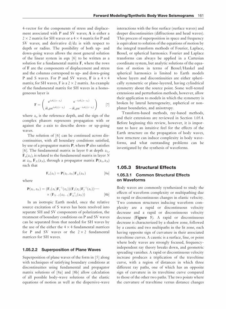
Body waves are commonly synthesized to study theeffects of waveform complexity or multipathing dueto rapid or discontinuous changes in elastic velocity.Two common structures inducing waveform com-plexity are a rapid or discontinuous velocitydecrease and a rapid or discontinuous velocitydecrease (Figure 5). A rapid or discontinuousdecrease is characterized by a shadow zone, followedby a caustic and two multipaths in the lit zone, eachhaving opposite sign of curvature in their associatedtraveltime curves. A caustic is a surface, line, or pointwhere body waves are strongly focused, frequency-independent ray theory breaks down, and geometricspreading vanishes. A rapid or discontinuous velocityincrease produces a triplication of the traveltimecurve, with a region of distances in which threedifferent ray paths, one of which has an oppositesign of curvature in its traveltime curve comparedto those of the other two paths. The two points wherethe curvature of traveltime versus distance changes


denote the distance at which the caustics intersect the

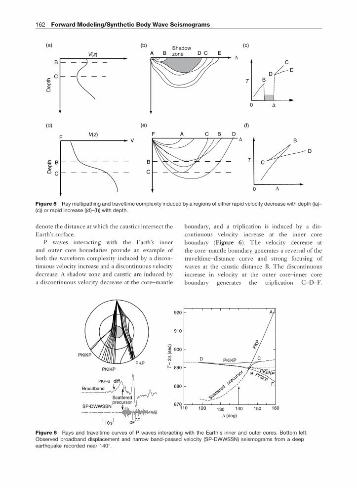
Earth’s surface.P waves interacting with the Earth’s inner

and outer core boundaries provide an example of

both the waveform complexity induced by a discon-

tinuous velocity increase and a discontinuous velocity

decrease. A shadow zone and caustic are induced by

a discontinuous velocity decrease at the core–mantle

boundary, and a triplication is induced by a dis-

continuous velocity increase at the inner core

boundary (Figure 6). The velocity decrease at

the core–mantle boundary generates a reversal of the

traveltime–distance curve and strong focusing of

waves at the caustic distance B. The discontinuous

increase in velocity at the outer core–inner core

boundary generates the triplication C–D–F.

PKP-B diff

Scatteredprecursor

DFCD

10 s

SP-DWWSSN

Broadband

PKiKP

PKIIKP

PKiKP

PKIKP

PKIKPPKP

PK

P

920

910

900

890

880

870110 120 130 140 150 160

Δ (deg)

T –

2Δ

(sec

)

Scatte

red precu

rsor

D C

F

B

A

Figure 6 Rays and traveltime curves of P waves interacting with the Earth’s inner and outer cores. Bottom left:

Observed broadband displacement and narrow band-passed velocity (SP-DWWSSN) seismograms from a deep

earthquake recorded near 140�.

V(z)

V(z)

B

C

B

C

B

C

FF

A C

C

CT

TD

E

B

D

B

Dep

thD

epth

VD

EDBAShadowzone

Δ

Δ

Δ

Δ

(e) (f)

(c)(b)(a)

(d)

C

B

0

0

Figure 5 Ray multipathing and traveltime complexity induced by a regions of either rapid velocity decrease with depth ((a)–(c)) or rapid increase ((d)–(f)) with depth.


Frequency-dependent diffraction occurs along the

extension of BC to shorter distance. A lower-amplitude

partial reflection along the dashed segment extends

from D to shorter distances. In addition to the effects

induced by radially symmetric structure, lateral het-

erogeneity near the core–mantle boundary can scatter

body waves in all directions. The curved dashed line

extended to shorter distances from point B in Figure 6

represents the minimum arrival time of high-fre-

quency energy scattered from either heterogeneity

near or topography on the core–mantle boundary.Changes in the curvature of traveltime curves for

waves also induce changes in the shapes of the waves

associated with each multipath. These waveform dis-

tortions can be understood from geometric spreading

effects. In an inhomogeneous medium, geometric

spreading R is proportional to the square root of the

product of the principal radii of curvature of the

wave front,

R _ffiffiffiffiffiffiffiffiffir 1r 2p ½9�

In a homogeneous medium, where wave fronts arespherical, r1¼ r2, and geometric spreading reduces

simply to the distance to the source. A wave front is

described by a 3-D surface �(x) over which travel-

time is constant. Hence, the principal radii of

curvature of the wave front are determined by the

second spatial derivatives of the traveltime surface � .

From [9], a change in the sign of either of the two

principal wave front curvatures ðr1 or r2Þ produces a

change in the sign of the argument of the square root

in [9] and hence a �/2 phase change in the waveform

associated with that wave front. A consequence of this

relation is that any two waveforms having traveltime

branches with a difference in the sign of the second

derivative with respect to great circle distance, will

differ by �/2 in phase. This �/2 phase change is

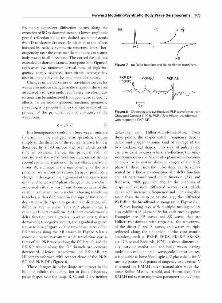
called a Hilbert transform. A Hilbert transform of a

delta function has a gradual positive onset, sharp

downswing to negative values, and a gradual negative

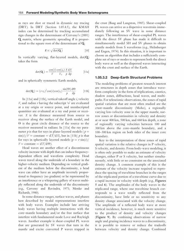
return to zero (Figure 7). The traveltime curve of the

PKP waves along the AB branch in Figure 6 has a

concave upward curvature, while travel time curva-

tures of the PKP waves along the BC branch and the

PKIKP waves along the DF branch are concave

downward. Hence, waveforms of PKP-AB are

Hilbert transformed with respect those of the PKP-

BC and PKP-DF (Figure 8).These changes in pulse shape are correct in the

limit of infinite frequency, but at finite frequency

pulse shapes near the cusps B, C, and D are neither

delta-like nor Hilbert-transformed-like. Near

these points, the shapes exhibit frequency depen-

dence and appear as some kind of average of the

two fundamental shapes. This type of pulse shape

can also exist in cases where a reflection/transmis-

sion/conversion coefficient of a plane wave becomes

complex, as in certain distance ranges of the SKS

phase. In these cases, the pulse shape can be repre-

sented by a linear combination of a delta function

and Hilbert-transformed delta function (Aki and

Richards, 1980, pp. 157–158). In the shadows of

cusps and caustics, diffracted waves exist, which

decay with increasing frequency and increasing dis-

tance from the cusp or caustic (e.g., the diffracted

PKP-B in the broadband seismogram in Figure 6).Waves having rays with multiple turning points

also exhibit �/2 phase shifts for each turning point.

Examples are PP waves and SS waves that are

Hilbert-transformed with respect to the waveforms

of the direct P and S waves, and waves multiply

reflected along the underside of the core mantle

boundary, such as PKKP, SKKS, PKnKP, SKnKS,

etc. (Choy and Richards, 1975). In three-dimension-

ally varying media and for body waves having

multiple turning points in waveguide-like structures,

it is possible to have N multiple �/2 phase shifts for N

turning points or N points of tangency to a caustic. N

is termed the KMAH index (named after wave the-

orists Keller, Maslov, Arnold, and Hormander). The

KMAH index is an important parameter to inventory

t

(a) (b)

t = 0

t = 0

πt–1

Figure 7 (a) Delta function and (b) its Hilbert transform.

6 s

PKP-DF(PKIKP)

PKP-BC PKP-AB

Figure 8 Observed and synthesized PKP waveforms from

Choy and Cormier (1993). PKP-AB is Hilbert-transformedwith respect to PKP-DF.


as rays are shot or traced in dynamic ray tracing(DRT). In DRT (Section 1.05.4.5), the KMAHindex can be determined by tracking accumulatedsign changes in the determinant of Cerveny’s (2001)Q matrix, where geometric spreading R is propor-tional to the square root of the determinant of Q:

R _

ffiffiffiffiffiffiffiffiffiffiffiffiffiffiffidetðQ Þ

p½10�

In vertically varying, flat-layered models, det(Q)takes the form

detðQ Þ ¼ cosðiÞV

cosðioÞVo

X

p

dX

dp½11a�

and in spherically symmetric Earth models,

detðQ Þ ¼ ðr roÞ2cosðiÞcosðioÞsinð�Þ

p

d�

dp½11b�

In [11a] and [11b], vertical takeoff angle i, velocityV, and radius r having the subscript ‘o’ are evaluatedat a ray origin or source point, and unsubscriptedquantities are evaluated at a ray end point or recei-ver. X is the distance measured from source toreceiver along the surface of the Earth model, and� is the great circle distance of the source to thereceiver measured in radians. In [11a] the ray para-meter p is that for rays in plane-layered models ( p ¼sin(i)/V ¼ constant ¼ dT/dX), but in [11b] p is thatfor rays in spherically layered models (p ¼ r sin(i)/V¼ constant ¼ dT/d�).

Head waves are another effect of a discontinuousvelocity increase with depth that can induce frequency-dependent effects and waveform complexity. Headwaves travel along the underside of a boundary in thehigher-velocity medium. Depending on vertical gradi-ent of the medium below the discontinuity, a headwave can either have an amplitude inversely propor-tional to frequency (no gradient) or be represented byan interference or a whispering gallery of waves multi-ply reflected along the underside of the discontinuity(e.g., Cerveny and Ravindra, 1971; Menke andRichards, 1980).

In some distance ranges, surface waves, and phasesbest described by modal representations interferewith body waves. Examples include late arrivingbody waves having multiple interactions with thecore–mantle boundary and/or the free surface thatinterfere with fundamental mode Love and Rayleighwaves. Another example is shear-coupled PL wavesthat are generated by SV waves that turn in themantle and excite converted P waves trapped in

the crust (Baag and Langston, 1985). Shear-coupledPL waves can arrive as a dispersive wavetrain imme-diately following an SV wave in some distanceranges. The interference of shear-coupled PL waveswith the direct SV phase has made it difficult tosimultaneously model SH and SV phases to obtainmantle models from S waveforms (e.g., Helmbergerand Engen, 1974). In this situation, it is important tochoose an algorithm that includes a sufficiently com-plete set of rays or modes to represent both the directbody wave as well as the dispersed waves interactingwith the crust and surface of the Earth.

1.05.3.2 Deep-Earth Structural Problems

The modeling problems of greatest research interestare structures in depth zones that introduce wave-form complexity in the form of triplications, caustics,shadow zones, diffractions, head waves, and multi-paths. For teleseismic observations, the zones of rapidspatial variation that are most often studied are thecrust–mantle discontinuity (Moho), a regionallyvarying low-velocity zone in the upper mantle, nar-row zones or discontinuities in velocity and densityat or near 400 km, 500 km, and 660 km depth, a zoneof regionally varying velocities between 100 and300 km above the core–mantle boundary, and a100–300 km region on both sides of the inner coreboundary.

Key to the interpretation of these zones of rapidspatial variation is the relative changes in P velocity,S velocity, and density. From body-wave modeling, itis often only possible to make an estimate of velocitychanges, either P or S velocity, but neither simulta-neously, with little or no constraint on the associateddensity change. A common example of this is theestimate of the velocity increase required to repro-duce the spacing of traveltime branches in the rangesof the triplicated portion of a traveltime curve due toa rapid increase in velocity with depth (e.g., Figures5 and 6). The amplitudes of the body waves in thetriplicated range, where one traveltime branch cor-responds to a wave totally reflected from thediscontinuity, have little or no sensitivity to anydensity change associated with the velocity change.The amplitude of a reflected body wave at morevertical incidence, however, is much more sensitiveto the product of density and velocity changes(Figure 9). By combining observations of narrowangle and grazing incidence waves to a discontinuity,it is possible to remove or reduce the tradeoffsbetween velocity and density change. Combined


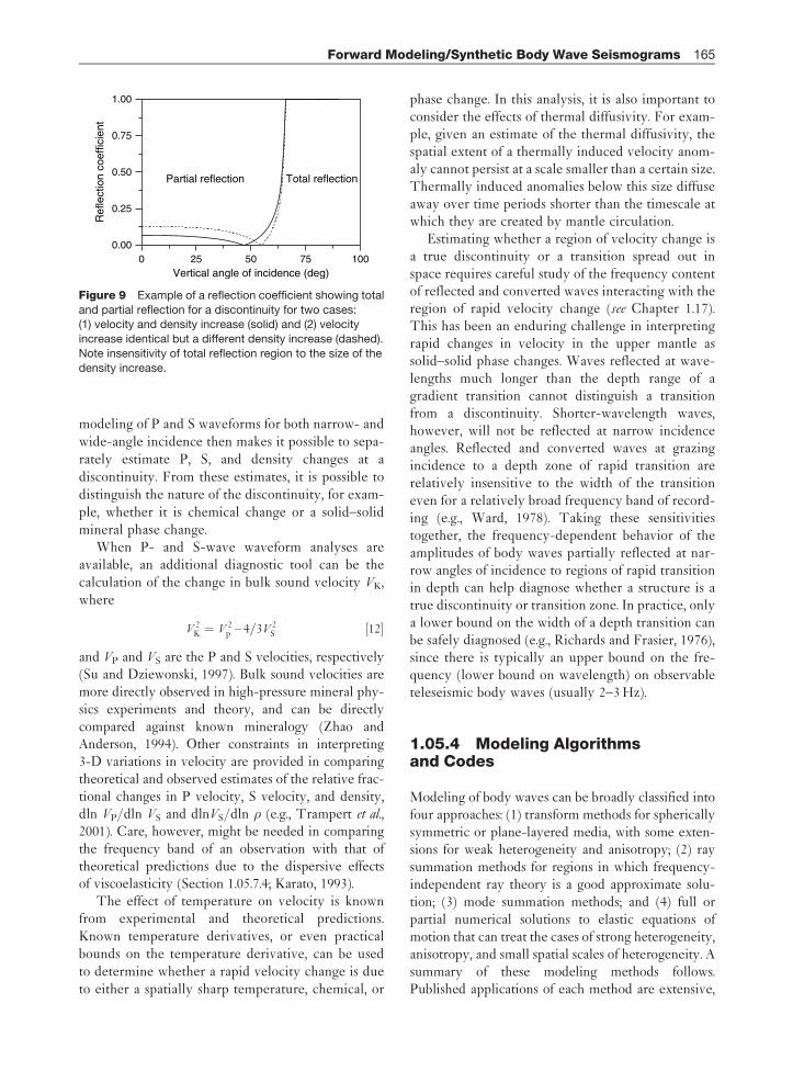
modeling of P and S waveforms for both narrow- andwide-angle incidence then makes it possible to sepa-rately estimate P, S, and density changes at adiscontinuity. From these estimates, it is possible todistinguish the nature of the discontinuity, for exam-ple, whether it is chemical change or a solid–solidmineral phase change.

When P- and S-wave waveform analyses areavailable, an additional diagnostic tool can be thecalculation of the change in bulk sound velocity VK,where

V 2K ¼ V 2

p – 4=3V 2S ½12�

and VP and VS are the P and S velocities, respectively(Su and Dziewonski, 1997). Bulk sound velocities aremore directly observed in high-pressure mineral phy-sics experiments and theory, and can be directlycompared against known mineralogy (Zhao andAnderson, 1994). Other constraints in interpreting3-D variations in velocity are provided in comparingtheoretical and observed estimates of the relative frac-tional changes in P velocity, S velocity, and density,dln VP/dln VS and dlnVS/dln � (e.g., Trampert et al.,2001). Care, however, might be needed in comparingthe frequency band of an observation with that oftheoretical predictions due to the dispersive effectsof viscoelasticity (Section 1.05.7.4; Karato, 1993).

The effect of temperature on velocity is knownfrom experimental and theoretical predictions.Known temperature derivatives, or even practicalbounds on the temperature derivative, can be usedto determine whether a rapid velocity change is dueto either a spatially sharp temperature, chemical, or

phase change. In this analysis, it is also important toconsider the effects of thermal diffusivity. For exam-ple, given an estimate of the thermal diffusivity, thespatial extent of a thermally induced velocity anom-aly cannot persist at a scale smaller than a certain size.Thermally induced anomalies below this size diffuseaway over time periods shorter than the timescale atwhich they are created by mantle circulation.

Estimating whether a region of velocity change isa true discontinuity or a transition spread out inspace requires careful study of the frequency contentof reflected and converted waves interacting with theregion of rapid velocity change (see Chapter 1.17).This has been an enduring challenge in interpretingrapid changes in velocity in the upper mantle assolid–solid phase changes. Waves reflected at wave-lengths much longer than the depth range of agradient transition cannot distinguish a transitionfrom a discontinuity. Shorter-wavelength waves,however, will not be reflected at narrow incidenceangles. Reflected and converted waves at grazingincidence to a depth zone of rapid transition arerelatively insensitive to the width of the transitioneven for a relatively broad frequency band of record-ing (e.g., Ward, 1978). Taking these sensitivitiestogether, the frequency-dependent behavior of theamplitudes of body waves partially reflected at nar-row angles of incidence to regions of rapid transitionin depth can help diagnose whether a structure is atrue discontinuity or transition zone. In practice, onlya lower bound on the width of a depth transition canbe safely diagnosed (e.g., Richards and Frasier, 1976),since there is typically an upper bound on the fre-quency (lower bound on wavelength) on observableteleseismic body waves (usually 2–3 Hz).

1.05.4 Modeling Algorithmsand Codes

Modeling of body waves can be broadly classified intofour approaches: (1) transform methods for sphericallysymmetric or plane-layered media, with some exten-sions for weak heterogeneity and anisotropy; (2) raysummation methods for regions in which frequency-independent ray theory is a good approximate solu-tion; (3) mode summation methods; and (4) full orpartial numerical solutions to elastic equations ofmotion that can treat the cases of strong heterogeneity,anisotropy, and small spatial scales of heterogeneity. Asummary of these modeling methods follows.Published applications of each method are extensive,

0 25 50 75 1000.00

0.25

0.50

0.75

1.00

Vertical angle of incidence (deg)

Ref

lect

ion

coef

ficie

nt

Partial reflection Total reflection

Figure 9 Example of a reflection coefficient showing total

and partial reflection for a discontinuity for two cases:(1) velocity and density increase (solid) and (2) velocity

increase identical but a different density increase (dashed).

Note insensitivity of total reflection region to the size of the

density increase.


and an attempt is made to primarily cite material inwhich the theory of each method is most completelydeveloped. In many cases, this will be a textbookrather than a journal paper. Good starting points toobtain software for many approaches are the ORFEUSsoftware library, codes deposited with the World DataCenter as part of the Seismological Algorithms text, codesand tutorials by R. Hermann, example synthetics andcodes distributed by the COSY Project, codes distrib-uted on a CD supplied with the International Handbook

for Earthquake and Engineering Seismology (Lee et al.,2001), and computational seismology software avail-able from the Computational Infrastructure inGeodynamics (CIG) web page.

1.05.4.1 Reflectivity

Reflectivity (Fuchs and Muller, 1971; Muller, 1985;Kind, 1985; Kennett, 1983, 2001) is perhaps the mostgeneral and popular transform method of modelingseismograms in radially symmetric or plane-layeredEarth models. Planar homogeneous layers parame-trize the Earth model, after an Earth-flatteningapproximation (EFA) is applied. Plane-wave solu-tions of the wave equation are found in thefrequency domain, with boundary conditionshandled by propagator matrix techniques. Thisapproach is used to derive a transformed solution atgreat circle distance �o for displacement, u(!, p,�o), in ray parameter and frequency space, where p

is related to the horizontal component of the wave-number vector by kz ¼ !p

re, with re the mean spherical

radius of the Earth. The solution U(t, �o) is thenfound by inverting Fourier transforms represented by

Uð!; �oÞ ¼1

2�

Z 1–1

d!e – i!t

Z�

dp uð!; p; �oÞ ½13�

Transform inversion is commonly accomplished byintegrating u(!, p, �o) along a contour D confined to afinite segment of the real p or kx axis for the series ofdiscrete 2N frequencies required to invert the complexfrequency spectrum by a fast Fourier transform (FFT).

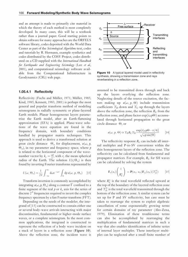
Depending on the needs of the modeler, the inte-grand of [13] can be constructed to contain either oneor several body-wave arrivals interacting with majordiscontinuities, fundamental or higher-mode surfacewaves, or a complete seismogram. In the most com-mon applications, the integrand is constructed torepresent the reflection of a body wave incident ona stack of layers in a reflection zone (Figure 10).Above the reflection zone, the incident wave is

assumed to be transmitted down through and backup the layers overlying the reflection zone.Neglecting details of the source excitation, the fac-tors making up uð!; p; �Þ include transmissioncoefficients TD down and TU up through the layersabove the reflection zone, the reflection RU from thereflection zone, and phase factor expði!p�Þ accumu-lated through horizontal propagation to the greatcircle distance �, or

uð!; p; �Þ _ TDRUTDexp½ið!p� – �=4Þ�ffiffiffiffiffiffiffiffiffiffiffiffiffiffiffiffiffiffiffi

!p sinð�Þp ½14�

The reflectivity response RU can include all inter-nal multiples and P-to-SV conversions within the

thin homogeneous layers of the reflection zone. Thereflectivity can be calculated from fundamental andpropagator matrices. For example, RU for SH wavescan be calculated by solving the system

Foðz1Þ1

R oU

!¼ Pðz1; zN ÞFN ðzN ÞðT N

D Þ ½15�

where R oU is the total wavefield reflected upward at

the top of the boundary of the layered reflection zoneand T N

D is the total wavefield transmitted through thebottom of the reflection zone. A similar system can beset up for P and SV reflectivity, but care must betaken to rearrange the system to exploit algebraiccancellation of some exponentially growing termsfor certain domains of ray parameter (Abo-Zena,1979). Elimination of these troublesome termscan also be accomplished by rearranging themultiplication of fundamental matrices in such away that also enables identification of infinite seriesof internal layer multiples. These interlayer multi-ples can be neglected after a small finite number of

Source

zo

zs

zm

zn

h

Free surfaceReceiver

Transmittinginterfaces

Reflectingandtransmittinginterfaces

Δ

}}

Figure 10 A typical layered model used in reflectivitysynthesis, showing a transmission zone and rays

reverberating in a reflection zone.


reverberations (Kennett, 1983, 2001). Truncation ofthese internal multiples helps eliminate later-arrivingenergy that folds back into the finite time windowrequired given by finite-length Fourier transforms.An alternative approach to eliminate the acausalarrival of the late-arriving interlayer multiples is toadd a small imaginary part to each frequency –i/� inthe evaluation of the reflectivity response beforeinverting the Fourier transform (Kennett, 1979;Chapman, 2004, p. 361). Using the damping theoremof Fourier transforms, at each time point the invertedsignal is then multiplied by the exponential exp(t/� ).

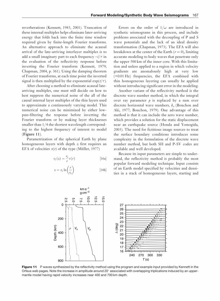
After choosing a method to eliminate acausal late-arriving multiples, one must still decide on how tobest suppress the numerical noise of the all of thecausal internal layer multiples of the thin layers usedto approximate a continuously varying model. Thisnumerical noise can be minimized by either low-pass-filtering the response before inverting theFourier transform or by making layer thicknessessmaller than 1/4 the shortest wavelength correspond-ing to the highest frequency of interest to model(Figure 11).

Parametrization of the spherical Earth by planehomogeneous layers with depth z first requires anEFA of velocities v(r) of the type (Muller, 1977)

vf ðzÞ ¼re

rvðrÞ ½16a�

z ¼ re lnr

re

� �½16b�

Errors on the order of 1/! are introduced insynthetic seismograms in this process, and includeproblems associated with the decoupling of P and Swave potentials and the lack of an ideal densitytransformation (Chapman, 1973). The EFA will alsobreakdown at the center of the Earth (r ¼ 0), limitingaccurate modeling to body waves that penetrate onlythe upper 500 km of the inner core. With this limita-tion and unless applied to a region in which velocitygradients are anomalously high at very low(<0.01 Hz) frequencies, the EFA combined withthin homogeneous layering can usually be appliedwithout introducing significant error in the modeling.

Another variant of the reflectivity method is thediscrete wave number method, in which the integralover ray parameter p is replaced by a sum overdiscrete horizontal wave numbers, kx (Bouchon andAki, 1977; Bouchon, 1979). One advantage of thismethod is that it can include the zero wave number,which provides a solution for the static displacementnear an earthquake source (Honda and Yomogida,2003). The need for fictitious image sources to treatthe surface boundary conditions introduces somecomplexity in the formulation of the discrete wavenumber method, but both SH and P-SV codes areavailable and well developed.

Because its input parameters are simple to under-stand, the reflectivity method is probably the mostpopular forward modeling technique. Input consistsof an Earth model specified by velocities and densi-ties in a stack of homogeneous layers, starting and

161718192021222324252627

240 270 300 330

2.5

5.0

7.5

10.0

12.5

15.0

200

0

400

600

800

Dep

th (

km)

ρ Vs Vp

km s–1

g cm–3

T (s)

Δ (d

eg)

Figure 11 P waves synthesized by the reflectivity method using the program and example input provided by Kennett in theOrfeus web pages. Note the increase in amplitude around 20� associated with overlapping triplications induced by an upper-

mantle model having rapid velocity increases near 400 and 700 km depth.


ending points of integration along a real ray para-meter axis, a time window and sampling rate, and asimple source description. Some 2-D extensions arenow available, allowing separate models to be speci-fied in the source and receiver regions (see Section1.05.7.1). Aside from simplicity of the input para-meters, an advantage of reflectivity is that it easilyallows the investigation of vertical transition zones inproperties modeled by arbitrarily thin layers. Thisadvantage, in common with all methods that allowfor the insertion of thin layers, can lead to the neglectof physical constraints on radial derivatives of elasticmoduli and density. Compared to ray-based methodsthat assume asymptotic approximations to verticalwave functions discussed in following sections,reflectivity can be numerically expensive for pro-blems requiring thousands of thin layers.

1.05.4.2 Generalized Ray

The method commonly dubbed the generalized raytechnique (GRT) originated from a technique ofhandling the integral transform inversions from rayparameter and frequency to time and space by theCagniard–de Hoop method. It was recognized thatmost important teleseismic arrivals can be calculatedby a first-motion approximation, allowing the timedomain solution for ray interactions in each layer,both reflected and head waves, to be solved analyti-cally (Helmberger 1974; Helmberger and Harkrider,1978). Ray solutions within each layer are summed,usually just the first multiples. The volume of pub-lished applications using the GRT method isprobably the largest of any other method, but itsavailable computer codes are less widely circulatedthan those employing reflectivity methods. An

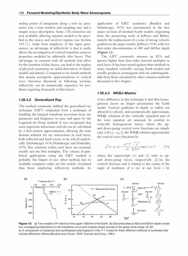
application of GRT synthetics (Burdick andHelmberger, 1978) was instrumental in the firstmajor revision of standard Earth models originatingfrom the pioneering work of Jeffreys and Bullen,namely the replacement of a zone of strong velocitygradient in the upper mantle (Jeffreys, 1936) with twofirst-order discontinuities at 400 and 660 km depth(Figure 12).

The GRT commonly assumes an EFA andignores higher than first-order internal multiples ineach layer. It has been tested against other methods inmany standard, vertically varying, Earth models andusually produces seismograms that are indistinguish-able from those calculated by other common methodsdiscussed in this chapter.

1.05.4.3 WKBJ-Maslov

A key difference in this technique is that thin homo-geneous layers no longer parametrize the Earthmodel. Vertical gradients in depth or radius areallowed in velocity, and asymptotically approximate,WKBJ, solutions of the vertically separated part ofthe wave equation are assumed. In contrast tovertically homogeneous layers, where the up-and down-going vertical wave functions are simplyexp½ �ikzðz – zref Þ�, the WKBJ solution approximates

the vertical wave functions by

gð1Þð2Þðr ; p; !Þ ¼ e�i�=4

!r

ffiffiffiffiffiffiffiffiffiV

�ðrÞ

sexpð� i! �Þ ½17a�

where the superscripts (1) and (2) refer to up-and down-going waves, respectively. �ðrÞis thevertical slowness and is related to the cosine of theangle of incidence of a ray at any level r by

200

400

600

800

Dep

th (

km)

P velocity (km s–1)

6.0

(a) (b) (c)

8.0 10.0 12.0

PEM-CT-7

0

70

60

50

12 16 20 24 28

D1

B1D2

B2

T-7 Reduced travel times

400 km

Δ = 23.5° Data LPZ

GRTSource

Δ = 27.1°

670 km

Reflectivity

Full wave

20 s

Source

T–1

0.8

∗ Δ

Figure 12 (a) Two models of P velocity in the upper 1000 km of the Earth. (b) Discontinuities at 400 and 650 km depth createtwo overlapping triplications in the traveltime curve and multiple phase arrivals in the great circle range 10–30�.(c) A comparison of observed and synthesized seismograms in the T-7 model for three different methods of synthesis that

include diffraction effects (Burdick and Orcutt, 1978; Cormier and Choy, 1981).


�ðrÞ ¼ cosðiÞ=V ¼ffiffiffiffiffiffiffiffiffiffiffiffiffiffiffiffiffiffiffiffiffiffiffiffiffiffi1=V 2 – p2=r 2

p. � is the delay

time obtained by integrating the vertical slownessfrom the radius turning point radius rp ,wherecos(i ) ¼ 0, to r :

� ¼Z r

rp

ffiffiffiffiffiffiffiffiffiffiffiffiffiffiffiffiffiffiffiffiffiffiffiffiffiffi1=V 2 – p2=r 2

p½17b�

The accuracy of these high-frequency approxima-tions increases as the ratio �/s decreases, where � isthe wavelength and s is the scale length of the med-ium. The scale length s is defined by

s ¼ minVS

rVSj j ;VP

rVp

�� ; �

r�j j ; rb

!½18�

where rb is the radius of curvature of a first-orderdiscontinuity in density or elastic velocity (Beydounand Ben-Menahem, 1985). Separability of P and Swave potentials is assumed in each inhomogeneouslayer, and frequency-dependent reflections andP-to-S conversions by regions of strong gradientsare ignored. Hence, transition zones, which may beof interest to mantle solid–solid phase changes,should be handled by thin layers of weaker gradientwhere the asymptotic approximations remain valid.For problems consisting of a body wave reflected byor bottoming above a discontinuity, the integrandu(!, p, �o) in [5] is replaced by

uð!; pÞ ¼ !1=2�ðpÞei!ðpÞ ½19a�

where

ð pÞ ¼Z r

rp

ffiffiffiffiffiffiffiffiffiffiffiffiffiffiffiffiffiffiffiffiffiffiffiffi1=v2 – p2=r 2

pþZ ro

rp

ffiffiffiffiffiffiffiffiffiffiffiffiffiffiffiffiffiffiffiffiffiffiffiffi1=v2 – p2=r 2

pþ p�o

½19b�

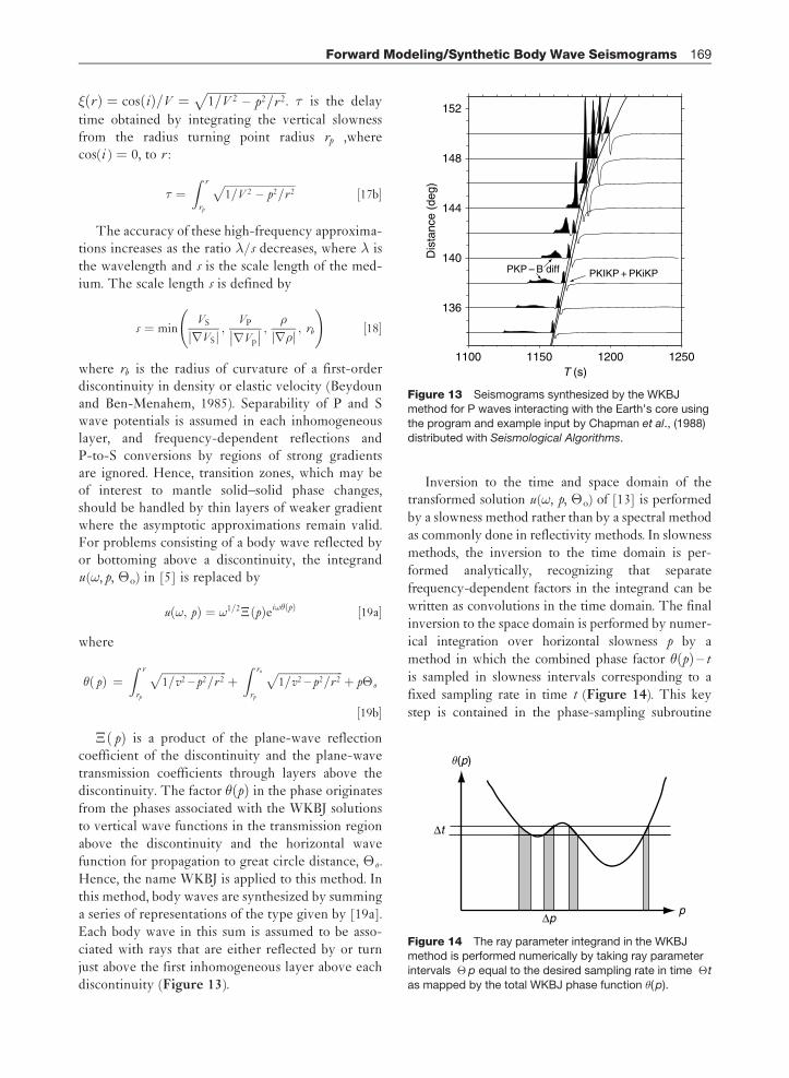
�ð pÞ is a product of the plane-wave reflectioncoefficient of the discontinuity and the plane-wavetransmission coefficients through layers above thediscontinuity. The factor ðpÞ in the phase originatesfrom the phases associated with the WKBJ solutionsto vertical wave functions in the transmission regionabove the discontinuity and the horizontal wavefunction for propagation to great circle distance, �o .Hence, the name WKBJ is applied to this method. Inthis method, body waves are synthesized by summinga series of representations of the type given by [19a].Each body wave in this sum is assumed to be asso-ciated with rays that are either reflected by or turnjust above the first inhomogeneous layer above eachdiscontinuity (Figure 13).

Inversion to the time and space domain of thetransformed solution u(!, p, �o) of [13] is performed

by a slowness method rather than by a spectral method

as commonly done in reflectivity methods. In slowness

methods, the inversion to the time domain is per-

formed analytically, recognizing that separate

frequency-dependent factors in the integrand can be

written as convolutions in the time domain. The final

inversion to the space domain is performed by numer-

ical integration over horizontal slowness p by a

method in which the combined phase factor ðpÞ – t

is sampled in slowness intervals corresponding to a

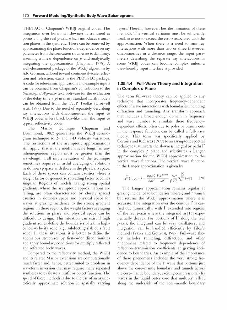
fixed sampling rate in time t (Figure 14). This key

step is contained in the phase-sampling subroutine

136

140

144

148

152

Dis

tanc

e (d

eg)

1100 1150 1200T (s)

1250

PKP – B diff PKIKP + PKiKP

Figure 13 Seismograms synthesized by the WKBJmethod for P waves interacting with the Earth’s core using

the program and example input by Chapman et al., (1988)

distributed with Seismological Algorithms.

θ(p)

Δt

Δpp

Figure 14 The ray parameter integrand in the WKBJmethod is performed numerically by taking ray parameter

intervals � p equal to the desired sampling rate in time �t

as mapped by the total WKBJ phase function ( p).


THETAC of Chapman’s WKBJ original codes. Theintegration over horizontal slowness is truncated atpoints along the real p-axis, which introduces trunca-tion phases in the synthetic. These can be removed byapproximating the phase function’s dependence on rayparameter from the truncation slownesses to�infinity,assuming a linear dependence on p, and analyticallyintegrating the approximation (Chapman, 1978). Awell-documented package of the WKBJ algorithm byA.R. Gorman, tailored toward continental-scale reflec-tion and refraction, exists in the PLOTSEC package.A code for teleseismic applications and example inputscan be obtained from Chapman’s contribution to theSeismological Algorithm text. Software for the evaluationof the delay time �(p) in many standard Earth modelscan be obtained from the TauP Toolkit (Crotwellet al., 1999). Due to the need of separately describingray interactions with discontinuities, the input toWKBJ codes is less black box-like than the input totypical reflectivity codes.

The Maslov technique (Chapman andDrummond, 1982) generalizes the WKBJ seismo-gram technique to 2- and 3-D velocity variations.The restrictions of the asymptotic approximationsstill apply, that is, the medium scale length in anyinhomogeneous region must be greater than thewavelength. Full implementation of the techniquesometimes requires an artful averaging of solutionsin slowness p space with those in the physical x space.Each of these spaces can contain caustics where aweight factor or geometric spreading factor becomessingular. Regions of models having strong spatialgradients, where the asymptotic approximations arefailing, are often characterized by closely spacedcaustics in slowness space and physical space forwaves at grazing incidence to the strong gradientregions. In these regions, the weight factors averagingthe solutions in phase and physical space can bedifficult to design. This situation can exist if highgradient zones define the boundaries of a thin high-or low-velocity zone (e.g., subducting slab or a faultzone). In these situations, it is better to define theanomalous structures by first-order discontinuitiesand apply boundary conditions for multiply reflectedand refracted body waves.

Compared to the reflectivity method, the WKBJand its related Maslov extensions are computationallymuch faster and, hence, better suited to problems inwaveform inversion that may require many repeatedsyntheses to evaluate a misfit or object function. Thespeed of these methods is due to the use of an asymp-totically approximate solution in spatially varying

layers. Therein, however, lies the limitation of thesemethods. The vertical variation must be sufficientlyweak so as not to exceed the errors associated with theapproximation. When there is a need to sum rayinteractions with more than two or three first-orderdiscontinuities in a distance range, the input para-meters describing the separate ray interactions insome WKBJ codes can become complex unless auser-friendly input interface is provided.

1.05.4.4 Full-Wave Theory and Integrationin Complex p Plane

The term full-wave theory can be applied to anytechnique that incorporates frequency-dependenteffects of wave interactions with boundaries, includingdiffraction and tunneling. Any transform approachthat includes a broad enough domain in frequencyand wave number to simulate these frequency-dependent effects, often due to poles or branch cutsin the response function, can be called a full-wavetheory. This term was specifically applied byCormier and Richards (1977) to an asymptotic spectraltechnique that inverts the slowness integral by paths D

in the complex p plane and substitutes a Langerapproximation for the WKBJ approximation to thevertical wave functions. The vertical wave functionin the Langer approximation is given by

gð1Þð2Þ ðr ; p; !Þ ¼ ��sVs

2�V

Vse�i�=6

!�

ffiffiffiffiffiffi!�

V �

rH

ð1Þð2Þ

1=3 ð!�Þ ½20�

The Langer approximation remains regular atgrazing incidence to boundaries where � and � vanishbut returns the WKBJ approximation where it isaccurate. The integration over the contour D is car-ried out numerically, with D extended into regionsoff the real p-axis where the integrand in [13] expo-nentially decays. For portions of D along the realp-axis, the integrand can be very oscillatory, andintegration can be handled efficiently by Filon’smethod (Frazer and Gettrust, 1985). Full-wave the-ory includes tunneling, diffraction, and otherphenomena related to frequency dependence ofreflection–transmission coefficients at grazing inci-dence to boundaries. An example of the importanceof these phenomena includes the very strong fre-quency dependence of the P wave that bottoms justabove the core–mantle boundary and tunnels acrossthe core–mantle boundary, exciting compressional (K)waves in the liquid outer core that multiply reflectalong the underside of the core–mantle boundary


(PKnKP waves; e.g., Richards (1973). Applying atten-tion to the validity of asymptotic approximations tothe Legendre function representing the phase effectsof propagating in the horizontal or � direction, full-wave theory has been extended to synthesize bodywaves that are strongly focused at the antipode bydiffraction around spherical boundaries from all azi-muths (Rial and Cormier, 1980).

The theory is most completely developed inchapter 9 of Aki and Richards (1981) and inSeismological Algorithms (Cormier and Richards,1988), where example codes and inputs are distribu-ted. As an asymptotic theory, full-wave theory sharesthe limitations of WKBJ codes, in that care must betaken not to assume too strong a velocity and densitygradient in each inhomogeneous layer. Added to thecomplexity in the description of ray interactionsshared with WKBJ code input, the construction offull-wave theory integrands and complex integrationpaths can be challenging, particularly for interferencehead wave and antipodal problems. Often it is best tostart with example input files specifying ray descrip-tions and integration paths for these problems, whichare distributed with Seismological Algorithms.

1.05.4.5 DRT and Gaussian Beams

DRT is simply a ray theory solution to the elasticequations of motion, consisting of a pulse arriving atthe least or stationary phase time, scaled by the ampli-tude factors due to plane-wave reflection andtransmission and geometric spreading. In an inhomo-geneous region, DRT solutions in the frequencydomain start from a trial solution in the form of factorsmultiplying inverse powers of radian frequency !:

uð!Þ ¼X

n

An

!nexpði!TÞ ½21�

The errors in the approximation given by n ¼ 0remain small for wavelengths much smaller than thescale length of the medium given by [18]. In practice,no more than the n¼ 0 term is ever calculated,because higher-order terms are expensive to calculateand can never properly include the frequency-dependent effects of waves reflected and convertedby regions of high spatial gradients in velocity anddensity. The review by Lambare and Virieux (thisvolume) provides further details on the derivation,accuracy, and frequency-dependent correctionsto asymptotic ray theory and also reviews the rela-tions between DRT, WKBJ/Maslov, and Gaussianbeam summation.

Superposition of Gaussian beams is an extensionof DRT and is closely related to the WKJB/Maslovtechniques. It amounts to a superposition of approxi-

mated wave fronts, weighted by a Gaussian-shapedwindow in space centered about each ray. The shapeof the wave front is estimated from the first and

second spatial derivatives of the wave front at theend point of each ray. This is referred to as a paraxial(close to the axis of the ray) approximation of the

wave front. To calculate the first- and second-orderspatial derivatives of the wave front, a system of

linear equations must be integrated. These equations,also required by DRT, consist of the kinematic equa-tions that describe the evolution of ray trajectory, its

vector slowness p, and traveltime, an equation todescribe the rotation of ray-centered coordinates in

which S-wave polarization remains fixed, and a sys-tem of equations for matrices P and Q needed todescribe the evolution of wave front curvature and

geometric spreading. The vector slowness p is simplythe spatial gradient of traveltime, and the geometric

spreading is related to the wave front curvature orsecond spatial derivatives of traveltime. When areceiver is not near a caustic, the quantities deter-

mined from integrating the DRT system can be usedto determine the frequency-dependent ray theory

solution, consisting of geometric spreading, travel-time, and products of reflection/transmissioncoefficients. The paraxially estimated phase from

the P and Q matrices of the DRT system can beused to either avoid two-point ray tracing by spa-tially extrapolating the traveltime near a ray or to

iteratively solve the two-point ray-tracing problem.The traveltime at a point x in the vicinity of a ray end

point at xo can be estimated by:

TðxÞ ¼ TðxoÞ þ p?�x þ 1

2�xt Ht MH�x ½22�

where

M ¼ PQ – 1 and

�x ¼ x – xo

The 2� 2 matrices P and Q are determined byintegrating the systems

dP

ds¼ VQ

dQ

ds¼ vP

½23�

along the ray paths. In [22], H is the transformationbetween ray-centered coordinates to Cartesian


coordinates. The columns of H are the vector basis ofthe ray-centered coordinate system at the ray endpoint. V is a matrix of second spatial derivatives ofvelocity in the ray-centered coordinate system. Thematrix Q can also be used to calculate geometricspreading [10]. The system in [23] can be generalizedusing a propagator, fundamental matrix formulism,similar to that used for propagating the solution tovertically separated equations of motion, except thatin this system the solutions are quantities related towave front curvature and ray density rather thancomponents of displacement and stress.

Gaussian beams are defined by adding a smallimaginary part to the matrix M in the paraxiallyextrapolated phase in [22], which gives an exponen-tial decay of a beam in space away from the centralray. The amplitude of each beam is proportional toreal part of exp(i!T), where T is made complex in[22] by the inclusion of a complex M. Beam summa-tion remains regular in the vicinity of ray caustics,where geometric spreading vanishes and ray theorysolutions become singular. It supplies estimates offrequency-dependent diffraction in the shadow ofcaustics and grazing incidence to boundaries.

To properly model classical head waves, somecare must be used in the design of beam weightingand beam widths. Weight factors of beams are deter-mined such that a superposition of beams returns aray theory solution for the complex spectrum, that is,U(!, x) ¼ exp(i!T)/sqrt(det(Q)), under a stationaryphase approximation to an integral over ray parameteror take-off angles. Like the WKBJ/Maslov solution,Gaussian beams give a nonsingular approximation tothe solution of the wavefield near a caustic.Restrictions on the validity of the method tend to besimilar to that of the WKBJ/Maslov method. Thescale length of the medium needs to be much largerthan the wavelength and also larger than the beamwidths (Ben-Menahem and Beydoun, 1985).

Compared to the Maslov technique, superpositionof Gaussian beams has less mathematical supportunless formulated in terms of complex rays as insome electromagnetic wave applications (Felsen,1984). For grazing incidence to regions of strongvelocity gradient, the paraxial approximation quicklyfails and caustics become closely spaced, making itdifficult to design optimal beam widths such that theparaxial approximation has small error in regions offthe central ray where some beams may still havelarge amplitude.

The notational framework of the P and Qmatrices and the propagator matrix of the dynamic

ray-tracing system developed by Cerveny and his co-workers are powerful tools that can simplify thecoding and understanding of any problem requiringthe use of ray theory. The DRT notation can beexploited to calculate the integrand for Kirchhoffintegrals and the banana-shaped kernels needed forfrequency-dependent tomography.

Computer codes for superposition of Gaussianbeams and DRT can be obtained from Cerveny’sgroup at Charles University as well as the WorldData Center. The best-developed codes are tailoredto continental scale reflection–refraction problems.One version (ANRAY) is one of the rare codes thatcombines general anisotropy with 3-D variations.A teleseismic-oriented version of DRT and beamsummation was written by Davis and Henson(1993), with a user-friendly graphical interface.

1.05.4.6 Modal Methods

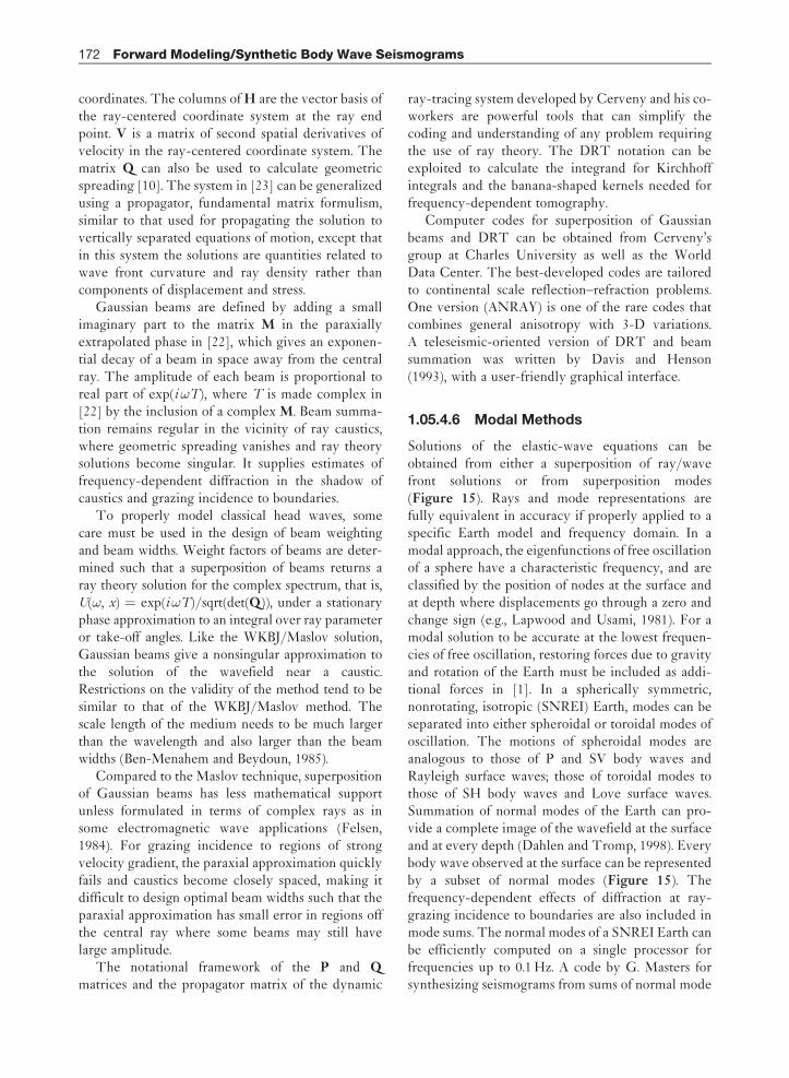
Solutions of the elastic-wave equations can beobtained from either a superposition of ray/wavefront solutions or from superposition modes(Figure 15). Rays and mode representations arefully equivalent in accuracy if properly applied to aspecific Earth model and frequency domain. In amodal approach, the eigenfunctions of free oscillationof a sphere have a characteristic frequency, and areclassified by the position of nodes at the surface andat depth where displacements go through a zero andchange sign (e.g., Lapwood and Usami, 1981). For amodal solution to be accurate at the lowest frequen-cies of free oscillation, restoring forces due to gravityand rotation of the Earth must be included as addi-tional forces in [1]. In a spherically symmetric,nonrotating, isotropic (SNREI) Earth, modes can beseparated into either spheroidal or toroidal modes ofoscillation. The motions of spheroidal modes areanalogous to those of P and SV body waves andRayleigh surface waves; those of toroidal modes tothose of SH body waves and Love surface waves.Summation of normal modes of the Earth can pro-vide a complete image of the wavefield at the surfaceand at every depth (Dahlen and Tromp, 1998). Everybody wave observed at the surface can be representedby a subset of normal modes (Figure 15). Thefrequency-dependent effects of diffraction at ray-grazing incidence to boundaries are also included inmode sums. The normal modes of a SNREI Earth canbe efficiently computed on a single processor forfrequencies up to 0.1 Hz. A code by G. Masters forsynthesizing seismograms from sums of normal mode


is included on the CD supplied with the International

Handbook for Earthquake and Engineering Seismology

(Lee, et al., 2001).An advantage of mode summation is that input

parameters are especially simple, basically just an

Earth model parametrization, a frequency band, and

desired number of modes. Mode summation is routi-nely used in the inversion of complete seismograms

to retrieve moment-tensor representations of earth-

quake sources (Dziewonski et al., 1981). A

disadvantage is that it is limited to lower frequencies

for practical computation on a single workstation.

Effects of gravity, Earth rotation, anisotropy, and

lateral heterogeneity remove degeneracy from

SNREI modes and couple spheroidal with toroidal

modes. Extensive literature exists on incorporation ofthe mode coupling induced by lateral heterogeneity

by applying perturbation techniques to SNREI

modes (e.g., Dahlen, 1987; Li and Tanimoto, 1993).Another modal-type approach is that of locked

modes (Figure 16). Here the modes are not whole-

Earth modes of free oscillation, but rather the surface-

wave modal energy that exponentially decays with

increasing depth from the surface. Modes are num-

bered by sign changes in displacement with depth,the zeroth mode corresponding to either the funda-

mental mode Love or Rayleigh surface wave. The

integrand u(!, p) in [13] must first be constructed to

include all interactions with the surface. The locked-

mode approach then evaluates the ray parameter or

wave number integral of [13] in the frequency

domain by deforming the integration contour in the

complex plane and applying the residue theorem tothe integrand. A high-velocity capping layer is placed

at depth, which locks plate-like modes into layers

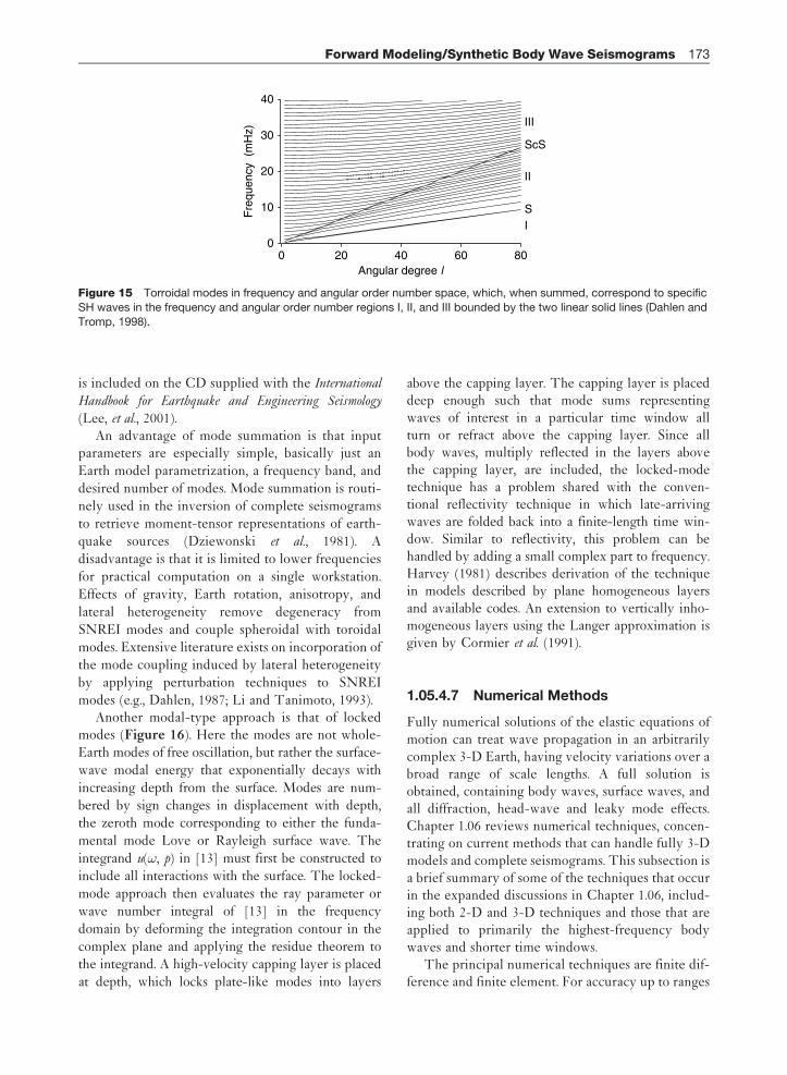
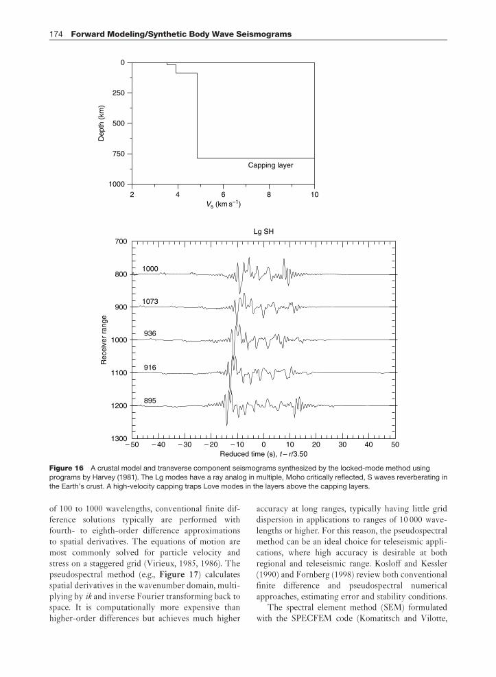
above the capping layer. The capping layer is placeddeep enough such that mode sums representingwaves of interest in a particular time window allturn or refract above the capping layer. Since allbody waves, multiply reflected in the layers abovethe capping layer, are included, the locked-modetechnique has a problem shared with the conven-tional reflectivity technique in which late-arrivingwaves are folded back into a finite-length time win-dow. Similar to reflectivity, this problem can behandled by adding a small complex part to frequency.Harvey (1981) describes derivation of the techniquein models described by plane homogeneous layersand available codes. An extension to vertically inho-mogeneous layers using the Langer approximation isgiven by Cormier et al. (1991).

1.05.4.7 Numerical Methods

Fully numerical solutions of the elastic equations ofmotion can treat wave propagation in an arbitrarilycomplex 3-D Earth, having velocity variations over abroad range of scale lengths. A full solution isobtained, containing body waves, surface waves, andall diffraction, head-wave and leaky mode effects.Chapter 1.06 reviews numerical techniques, concen-trating on current methods that can handle fully 3-Dmodels and complete seismograms. This subsection isa brief summary of some of the techniques that occurin the expanded discussions in Chapter 1.06, includ-ing both 2-D and 3-D techniques and those that areapplied to primarily the highest-frequency bodywaves and shorter time windows.

The principal numerical techniques are finite dif-ference and finite element. For accuracy up to ranges

ScS

II

III

0

10

20

30

40

0 20 40 60 80F

requ

ency

(m

Hz)

Angular degree l

SI

Figure 15 Torroidal modes in frequency and angular order number space, which, when summed, correspond to specific

SH waves in the frequency and angular order number regions I, II, and III bounded by the two linear solid lines (Dahlen and

Tromp, 1998).


of 100 to 1000 wavelengths, conventional finite dif-ference solutions typically are performed withfourth- to eighth-order difference approximationsto spatial derivatives. The equations of motion aremost commonly solved for particle velocity andstress on a staggered grid (Virieux, 1985, 1986). Thepseudospectral method (e.g., Figure 17) calculatesspatial derivatives in the wavenumber domain, multi-plying by ik and inverse Fourier transforming back tospace. It is computationally more expensive thanhigher-order differences but achieves much higher

accuracy at long ranges, typically having little griddispersion in applications to ranges of 10 000 wave-lengths or higher. For this reason, the pseudospectralmethod can be an ideal choice for teleseismic appli-cations, where high accuracy is desirable at bothregional and teleseismic range. Kosloff and Kessler(1990) and Fornberg (1998) review both conventionalfinite difference and pseudospectral numericalapproaches, estimating error and stability conditions.

The spectral element method (SEM) formulatedwith the SPECFEM code (Komatitsch and Vilotte,

700

800

900

1000

1000

1073

936

916

895

1100

1200

1300

Reduced time (s), t – r /3.50100

Lg SH

20 30 40 50– 50 – 40 – 30 – 20 – 10

Rec

eive

r ra

nge

10002 4 6

Vs (km s–1)8 10

750

500

250

0

Dep

th (

km)

Capping layer

Figure 16 A crustal model and transverse component seismograms synthesized by the locked-mode method using

programs by Harvey (1981). The Lg modes have a ray analog in multiple, Moho critically reflected, S waves reverberating in

the Earth’s crust. A high-velocity capping traps Love modes in the layers above the capping layers.


1998; Komatitsch and Tromp, 1999, 2002) is currentlyone of the few numeric methods designed to handlea fully 3-D Earth model. SPECFEM has a well-developed interface to grid the elements needed forarbitrarily complex 3-D models. Versions ofSPECFEM are available for both local/regional-scaleproblems for ranges on the order of 0–100 km, and forglobal- or teleseismic-scale problems. Another popularregional scale code is the elastic finite difference pro-gram by Larsen and Schultz (1995), which has beenapplied to the effects of 3-D basins and extended faultslip (e.g., Hartzell et al., 1999).

The direct solution method (DSM) is a numericaltechnique that numerically solves the equations ofmotion for a series of frequencies required for inver-sion to the time domain by an FFT (Cummins et al.,1994a, 1994b). The particular numerical techniqueconsists in expanding displacements in the frequencydomain by a series of basis functions consisting of a

product of splines in the vertical direction and sphe-rical harmonics in the angular direction. In somerespects, the use of basis functions is similar to pseu-dospectral methods that represent the spatialspectrum of model variations by Fourier or sphericalharmonic series. In DSM, the coefficients for thebasis functions are found by the method of weightedresiduals (Geller and Ohminato, 1994). The SH andP-SV seismograms be computed by DSM are com-plete, in that they contain all possible body andsurface waves. Hence, DSM is a viable alternativeto summing modes of free oscillation. Weak 3-Dperturbations to a radially symmetric backgroundmodel are possible in DSM at a computational costnot much higher than that required for the back-ground model (Takeuchi et al., 2000).

Computational time is a practical limitation tonumerical modeling. Since most numerical techni-ques require Earth models specified on a spatial gridor elements, it is straightforward to parallelize thecomputation by decomposing the spatial grid or ele-ments over multiple processors. Practicalcomputations can be defined by time required tocompute a problem. Depending on the algorithmand frequency band, common computer resourcesin most labs allow a complete teleseismic wavefieldto be synthesized in 1 or 2 days using 10–100 pro-cessors in parallel. Typical body waves having a highsignal-to-noise ratio in the teleseismic range(10–180�) exist up to 2 Hz. Practical 2-D modelingcan be currently performed at teleseismic range up to1 Hz with finite difference and pseudospectral meth-ods; 3-D problems with the SPECFEM finiteelement method can be done up to 0.1 Hz in thistime period with a similar number of processors. Atranges less than 100 km, 3-D problems can be practi-cally performed at frequencies up to 1 or 2 Hz (orderof 200 wavelengths). This range and frequency bandjust starts to cover the frequencies of interest tostrong ground motion. Frequencies up to 10 Hz at2000 km range (>5000 wavelengths) in complex 3-Dstructure are of interest to the problem of discrimi-nating earthquake sources from underground nucleartests. This is a research problem that is still inacces-sible with small to moderate size clusters (less than100 nodes) and numerical methods.

A large body of literature exists in the applicationof finite difference and pseudospectral solutions forlocal-scale problems up to 100 km for explorationapplications and strong ground motion applications(e.g., Harzell et al., 1999; Olsen, 2000) Significantlysmaller amounts of published work exists for

0 250 500 750 1000 1250 1500Time (s)

25

35

45

55

65

75

Dis

tanc

e (d

eg)

0

(a)

(b)

1925

3850

Distance (deg)

Fla

ttene

d de

pth

(km

)

S

ScS

sSsScS

SS

S

SS

ScS

sScS

SSS

0 20 40 60 80

Figure 17 Wave fronts (a) and complete transverse

(SH) component seismograms (b) synthesized by thepseudospectral method from Cormier (2000). Note the

increase in amplitudes occurring at roughly 20� intervals

in S, SS, and SSS due to rapid increases in velocity at

upper-mantle solid–solid phase transitions.


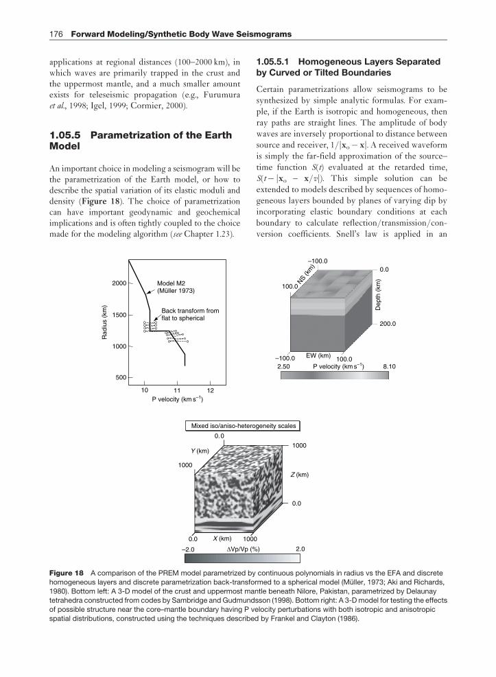
applications at regional distances (100–2000 km), inwhich waves are primarily trapped in the crust andthe uppermost mantle, and a much smaller amountexists for teleseismic propagation (e.g., Furumuraet al., 1998; Igel, 1999; Cormier, 2000).

1.05.5 Parametrization of the EarthModel

An important choice in modeling a seismogram will bethe parametrization of the Earth model, or how todescribe the spatial variation of its elastic moduli anddensity (Figure 18). The choice of parametrizationcan have important geodynamic and geochemicalimplications and is often tightly coupled to the choicemade for the modeling algorithm (see Chapter 1.23).

1.05.5.1 Homogeneous Layers Separatedby Curved or Tilted Boundaries

Certain parametrizations allow seismograms to be

synthesized by simple analytic formulas. For exam-

ple, if the Earth is isotropic and homogeneous, then

ray paths are straight lines. The amplitude of body

waves are inversely proportional to distance between

source and receiver, 1/jxo� xj. A received waveform

is simply the far-field approximation of the source–

time function S(t) evaluated at the retarded time,

S(t� jxo – x/vj). This simple solution can be

extended to models described by sequences of homo-

geneous layers bounded by planes of varying dip by

incorporating elastic boundary conditions at each

boundary to calculate reflection/transmission/con-

version coefficients. Snell’s law is applied in an

10 11 12

–100.00.0

100.0

100.0

200.0

Dep

th (

km)NS (k

m)

EW (km)

2.50–100.0

8.10P velocity (km s–1)

2000

1500

1000

500

P velocity (km s–1)

Rad

ius

(km

)

Model M2(Müller 1973)

Back transform fromflat to spherical

Mixed iso/aniso-heterogeneity scales

1000X (km)

0.0

1000

Z (km)

0.0

1000

Y (km)

–2.0 2.0ΔVp/Vp (%)

0.0

Figure 18 A comparison of the PREM model parametrized by continuous polynomials in radius vs the EFA and discrete

homogeneous layers and discrete parametrization back-transformed to a spherical model (Muller, 1973; Aki and Richards,

1980). Bottom left: A 3-D model of the crust and uppermost mantle beneath Nilore, Pakistan, parametrized by Delaunaytetrahedra constructed from codes by Sambridge and Gudmundsson (1998). Bottom right: A 3-D model for testing the effects

of possible structure near the core–mantle boundary having P velocity perturbations with both isotropic and anisotropic

spatial distributions, constructed using the techniques described by Frankel and Clayton (1986).


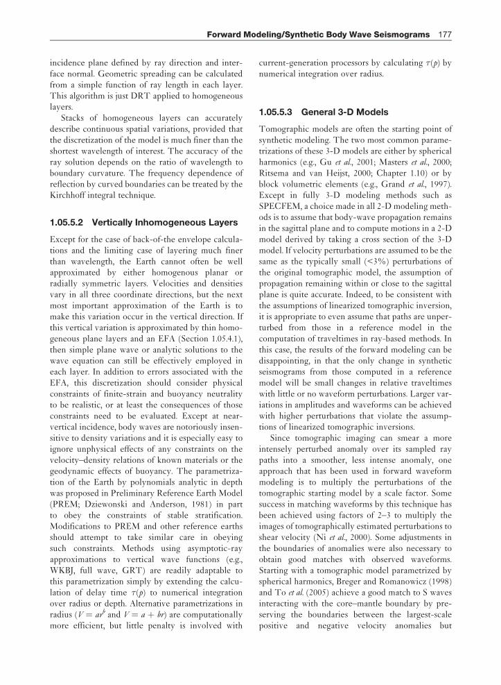
incidence plane defined by ray direction and inter-face normal. Geometric spreading can be calculatedfrom a simple function of ray length in each layer.This algorithm is just DRT applied to homogeneouslayers.

Stacks of homogeneous layers can accuratelydescribe continuous spatial variations, provided thatthe discretization of the model is much finer than theshortest wavelength of interest. The accuracy of theray solution depends on the ratio of wavelength toboundary curvature. The frequency dependence ofreflection by curved boundaries can be treated by theKirchhoff integral technique.

1.05.5.2 Vertically Inhomogeneous Layers

Except for the case of back-of-the envelope calcula-tions and the limiting case of layering much finerthan wavelength, the Earth cannot often be wellapproximated by either homogenous planar orradially symmetric layers. Velocities and densitiesvary in all three coordinate directions, but the nextmost important approximation of the Earth is tomake this variation occur in the vertical direction. Ifthis vertical variation is approximated by thin homo-geneous plane layers and an EFA (Section 1.05.4.1),then simple plane wave or analytic solutions to thewave equation can still be effectively employed ineach layer. In addition to errors associated with theEFA, this discretization should consider physicalconstraints of finite-strain and buoyancy neutralityto be realistic, or at least the consequences of thoseconstraints need to be evaluated. Except at near-vertical incidence, body waves are notoriously insen-sitive to density variations and it is especially easy toignore unphysical effects of any constraints on thevelocity–density relations of known materials or thegeodynamic effects of buoyancy. The parametriza-tion of the Earth by polynomials analytic in depthwas proposed in Preliminary Reference Earth Model(PREM; Dziewonski and Anderson, 1981) in partto obey the constraints of stable stratification.Modifications to PREM and other reference earthsshould attempt to take similar care in obeyingsuch constraints. Methods using asymptotic-rayapproximations to vertical wave functions (e.g.,WKBJ, full wave, GRT) are readily adaptable tothis parametrization simply by extending the calcu-lation of delay time �(p) to numerical integrationover radius or depth. Alternative parametrizations inradius (V ¼ arb and V ¼ a þ br) are computationallymore efficient, but little penalty is involved with

current-generation processors by calculating �(p) bynumerical integration over radius.

1.05.5.3 General 3-D Models

Tomographic models are often the starting point ofsynthetic modeling. The two most common parame-trizations of these 3-D models are either by sphericalharmonics (e.g., Gu et al., 2001; Masters et al., 2000;Ritsema and van Heijst, 2000; Chapter 1.10) or byblock volumetric elements (e.g., Grand et al., 1997).Except in fully 3-D modeling methods such asSPECFEM, a choice made in all 2-D modeling meth-ods is to assume that body-wave propagation remainsin the sagittal plane and to compute motions in a 2-Dmodel derived by taking a cross section of the 3-Dmodel. If velocity perturbations are assumed to be thesame as the typically small (<3%) perturbations ofthe original tomographic model, the assumption ofpropagation remaining within or close to the sagittalplane is quite accurate. Indeed, to be consistent withthe assumptions of linearized tomographic inversion,it is appropriate to even assume that paths are unper-turbed from those in a reference model in thecomputation of traveltimes in ray-based methods. Inthis case, the results of the forward modeling can bedisappointing, in that the only change in syntheticseismograms from those computed in a referencemodel will be small changes in relative traveltimeswith little or no waveform perturbations. Larger var-iations in amplitudes and waveforms can be achievedwith higher perturbations that violate the assump-tions of linearized tomographic inversions.

Since tomographic imaging can smear a moreintensely perturbed anomaly over its sampled raypaths into a smoother, less intense anomaly, oneapproach that has been used in forward waveformmodeling is to multiply the perturbations of thetomographic starting model by a scale factor. Somesuccess in matching waveforms by this technique hasbeen achieved using factors of 2–3 to multiply theimages of tomographically estimated perturbations toshear velocity (Ni et al., 2000). Some adjustments inthe boundaries of anomalies were also necessary toobtain good matches with observed waveforms.Starting with a tomographic model parametrized byspherical harmonics, Breger and Romanowicz (1998)and To et al. (2005) achieve a good match to S wavesinteracting with the core–mantle boundary by pre-serving the boundaries between the largest-scalepositive and negative velocity anomalies but


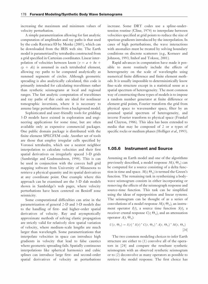
increasing the maximum and minimum values ofvelocity perturbation.

A simple parametrization allowing for fast analyticcomputation of amplitudes and ray paths is that usedby the code Raytrace3D by Menke (2005), which canbe downloaded from the IRIS web site. The Earthmodel is parametrized by tetrahedra constructed froma grid specified in Cartesian coordinates. Linear inter-polation of velocities between knots (v ¼ a þ bx þcy þ dz) is assumed in each tetrahedral element,allowing ray paths to be computed analytically assummed segments of circles. Although geometricspreading is also analytically calculated, this code isprimarily intended for calculating traveltimes ratherthan synthetic seismograms at local and regionalranges. The fast analytic computation of traveltimesand ray paths of this code are ideal for nonlineartomographic inversions, where it is necessary toassume large perturbations from a background model.

Sophisticated and user-friendly tools for gridding3-D models have existed in exploration and engi-neering applications for some time, but are oftenavailable only as expensive commercial packages.One public domain package is distributed with thefinite element SPECFEM code. Another set of toolsare those that employ irregular cells specified byVoronoi tetrahedra, which use a nearest neighborinterpolation to calculate velocities and their firstspatial derivatives on irregularly spaced 3-D grids(Sambridge and Gudmundsson, 1998). This is canbe used in conjunction with the convex hull gridmapping software from University of Minnesota toretrieve a physical quantity and its spatial derivativesat any coordinate point. One example where thisapproach can be examined are the 3-D slab modelsshown in Sambridge’s web pages, where velocityperturbations have been centered on Benioff zoneseismicity.

Some computational difficulties can arise in theparametrization of general 2-D and 3-D models dueto the handling of first- and higher-order spatialderivatives of velocity. Ray and asymptoticallyapproximate methods of solving elastic propagationare strictly valid for relatively slow spatial variationof velocity, where medium-scale lengths are muchlarger than wavelength. Some parametrizations thatinterpolate velocities in space can introduce highgradients in velocity that lead to false causticswhere geometric spreading fails. Spatially continuousinterpolations like spherical harmonics and cubicsplines can introduce large first- and second-orderspatial derivatives of velocity as perturbations

increase. Some DRT codes use a spline-under-tension routine (Cline, 1974) to interpolate betweenvelocities specified at grid points to reduce the size ofspurious gradients introduced by the interpolation. Incases of high perturbations, the wave interactionswith anomalies must be treated by solving boundaryconditions on discrete scatterers (e.g., Korneev andJohnson, 1993; Imhof and Toksoz, 2001).

Rapid advances in computation have made it pos-sible to more routinely include the effects ofheterogeneity on the scale of wavelengths usingnumerical finite difference and finite element meth-ods. It is usually impossible to deterministically knowfine-scale structure except in a statistical sense as aspatial spectrum of heterogeneity. The most commonway of constructing these types of models is to imposea random number generator at finite difference orelement grid points, Fourier transform the grid fromphysical space to wavenumber space, filter by anassumed spatial spectrum of heterogeneity, andinverse Fourier transform to physical space (Frankeland Clayton, 1986). This idea has been extended tomedia that may be composed of 2 or n types ofspecific rocks or medium phases (Holliger et al., 1993).

1.05.6 Instrument and Source

Assuming an Earth model and one of the algorithmspreviously described, a model response M(t, �o) canbe computed for a source consisting of a delta func-tion in time and space. M(t, �o) is termed the Green’sfunction. The remaining task in synthesizing a body-wave seismogram consists in either incorporating orremoving the effects of the seismograph response andsource-time function. This task can be simplifiedusing the ideas of superposition and linear systems.The seismogram can be thought of as a series ofconvolutions of a model response M(t, �o), an instru-ment operator I(t), a source time function S(t), areceiver crustal response C(t, �o), and an attenuationoperator A(t, �o):

Uðt ; �oÞ ¼ I ðtÞ � SðtÞ � Cðt ; �oÞ � Aðt ; �oÞ �Mðt ; �oÞ½24�

The two common modeling choices to infer Earthstructure are either to (1) convolve all of the opera-tors in [24] and compare the resultant syntheticseismogram with an observed synthetic seismogramor to (2) deconvolve as many operators as possible toretrieve the model response. The first choice has


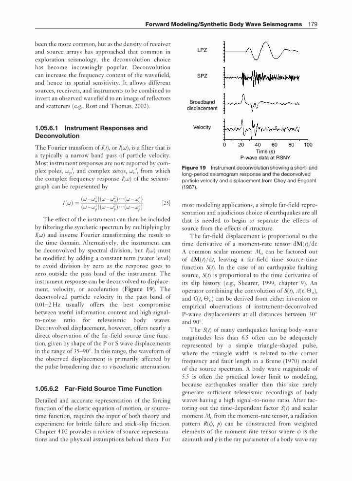
been the more common, but as the density of receiverand source arrays has approached that common inexploration seismology, the deconvolution choicehas become increasingly popular. Deconvolutioncan increase the frequency content of the wavefield,and hence its spatial sensitivity. It allows differentsources, receivers, and instruments to be combined toinvert an observed wavefield to an image of reflectorsand scatterers (e.g., Rost and Thomas, 2002).

1.05.6.1 Instrument Responses andDeconvolution

The Fourier transform of I(t), or I(!), is a filter that isa typically a narrow band pass of particle velocity.Most instrument responses are now reported by com-plex poles, !p

i, and complex zeros, !oi, from which

the complex frequency response I(!) of the seismo-graph can be represented by

I ð!Þ ¼ ð! –!1oÞð! –!2

oÞ???ð! –!noÞ

ð! –!1pÞð! –!2

pÞ???ð! –!npÞ

½25�

The effect of the instrument can then be includedby filtering the synthetic spectrum by multiplying byI(!) and inverse Fourier transforming the result tothe time domain. Alternatively, the instrument canbe deconvolved by spectral division, but I(!) mustbe modified by adding a constant term (water level)to avoid division by zero as the response goes tozero outside the pass band of the instrument. Theinstrument response can be deconvolved to displace-ment, velocity, or acceleration (Figure 19). Thedeconvolved particle velocity in the pass band of0.01–2 Hz usually offers the best compromisebetween useful information content and high signal-to-noise ratio for teleseismic body waves.Deconvolved displacement, however, offers nearly adirect observation of the far-field source time func-tion, given by shape of the P or S wave displacementsin the range of 35–90�. In this range, the waveform ofthe observed displacement is primarily affected bythe pulse broadening due to viscoelastic attenuation.

1.05.6.2 Far-Field Source Time Function

Detailed and accurate representation of the forcingfunction of the elastic equation of motion, or source-time function, requires the input of both theory andexperiment for brittle failure and stick-slip friction.Chapter 4.02 provides a review of source representa-tions and the physical assumptions behind them. For

most modeling applications, a simple far-field repre-sentation and a judicious choice of earthquakes are allthat is needed to begin to separate the effects ofsource from the effects of structure.

The far-field displacement is proportional to thetime derivative of a moment-rate tensor dM(t)/dt.A common scalar moment Mo can be factored outof dM(t)/dt, leaving a far-field time source-timefunction S(t). In the case of an earthquake faultingsource, S(t) is proportional to the time derivative ofits slip history (e.g., Shearer, 1999, chapter 9). Anoperator combining the convolution of S(t), A(t, �o),and C(t, �o) can be derived from either inversion orempirical observations of instrument-deconvolvedP-wave displacements at all distances between 30�

and 90� .The S(t) of many earthquakes having body-wave

magnitudes less than 6.5 often can be adequatelyrepresented by a simple triangle-shaped pulse,where the triangle width is related to the cornerfrequency and fault length in a Brune (1970) modelof the source spectrum. A body wave magnitude of5.5 is often the practical lower limit to modeling,because earthquakes smaller than this size rarelygenerate sufficient teleseismic recordings of bodywaves having a high signal-to-noise ratio. After fac-toring out the time-dependent factor S(t) and scalarmoment Mo from the moment-rate tensor, a radiationpattern R(, p) can be constructed from weightedelements of the moment-rate tensor where is theazimuth and p is the ray parameter of a body wave ray

0

LPZ

SPZ

Broadbanddisplacement

Velocity

Time (s)P-wave data at RSNY

20 40 60 80 100

Figure 19 Instrument deconvolution showing a short- andlong-period seismogram response and the deconvolved

particle velocity and displacement from Choy and Engdahl

(1987).


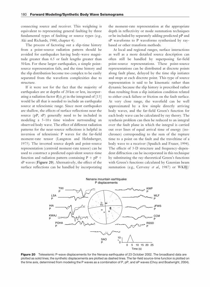
connecting source and receiver. This weighting isequivalent to representing general faulting by three

fundamental types of faulting or source types (e.g.,

Aki and Richards, 1980, chapter 4).The process of factoring out a slip-time history

from a point-source radiation pattern should be

avoided for earthquakes having body-wave magni-tude greater than 6.5 or fault lengths greater than

50 km. For these larger earthquakes, a simple point-

source representation fails, and the time history andthe slip distribution become too complex to be easily

separated from the waveform complexities due tostructure.

If it were not for the fact that the majority ofearthquakes are at depths of 20 km or less, incorpor-ating a radiation factor R(, p) in the integrand of [13]

would be all that is needed to include an earthquake

source at teleseismic range. Since most earthquakesare shallow, the effects of surface reflections near the

source (pP, sP) generally need to be included inmodeling a 5–10 s time window surrounding an

observed body wave. The effect of different radiationpatterns for the near-source reflections is helpful in

inversion of teleseismic P waves for the far-fieldmoment-rate tensor (Langston and Helmberger,

1975). The inverted source depth and point-source

representation (centroid moment-rate tensor) can beused to construct a predicted equivalent source-time

function and radiation pattern containing P þ pP þsP waves (Figure 20). Alternatively, the effect of the

surface reflections can be handled by incorporating

the moment-rate representation at the appropriatedepth in reflectivity or mode summation techniquesor be included by separately adding predicted pP and

sP waveforms to P waveforms synthesized by ray-based or other transform methods.

At local and regional ranges, surface interactionsas well as a more detailed source description canoften still be handled by superposing far-fieldpoint-source representations. These point-source

representations can be distributed at discrete pointsalong fault plane, delayed by the time slip initiatesand stops at each discrete point. This type of source

representation is said to be kinematic rather thandynamic because the slip history is prescribed ratherthan resulting from a slip initiation condition relatedto either crack failure or friction on the fault surface.

At very close range, the wavefield can be wellapproximated by a few simple directly arrivingbody waves, and the far-field Green’s function for

each body wave can be calculated by ray theory. Thesynthesis problem can then be reduced to an integralover the fault plane in which the integral is carriedout over lines of equal arrival time of energy (iso-

chrones) corresponding to the sum of the rupturetime to a point on the fault and the traveltime of abody wave to a receiver (Spudich and Frazer, 1994).

The effects of 3-D structure and frequency-depen-dent diffraction can be incorporated in this techniqueby substituting the ray-theoretical Green’s functionswith Green’s functions calculated by Gaussian beam

summation (e.g., Cerveny et al., 1987) or WKBJ/

Nenana mountain earhtquakeP displacements

TIXIP

LSAP

HIAP

KWAJP

SAOP

POHAP

RSSDP

CCMP

JFWSP

WLFP

KWPP

10

00 5 10

Time (s)

μ

15 20 25

Figure 20 Teleseismic P-wave displacements for the Nenana earthquake of 23 October 2002. The broadband data are

plotted as solid lines; the synthetic displacements are plotted as dashed lines. The far-field source-time function is plotted on

the time axis, determined from modeling the P waves as a combination of P, pP, and sP waves (Choy and Boatwright, 2004).


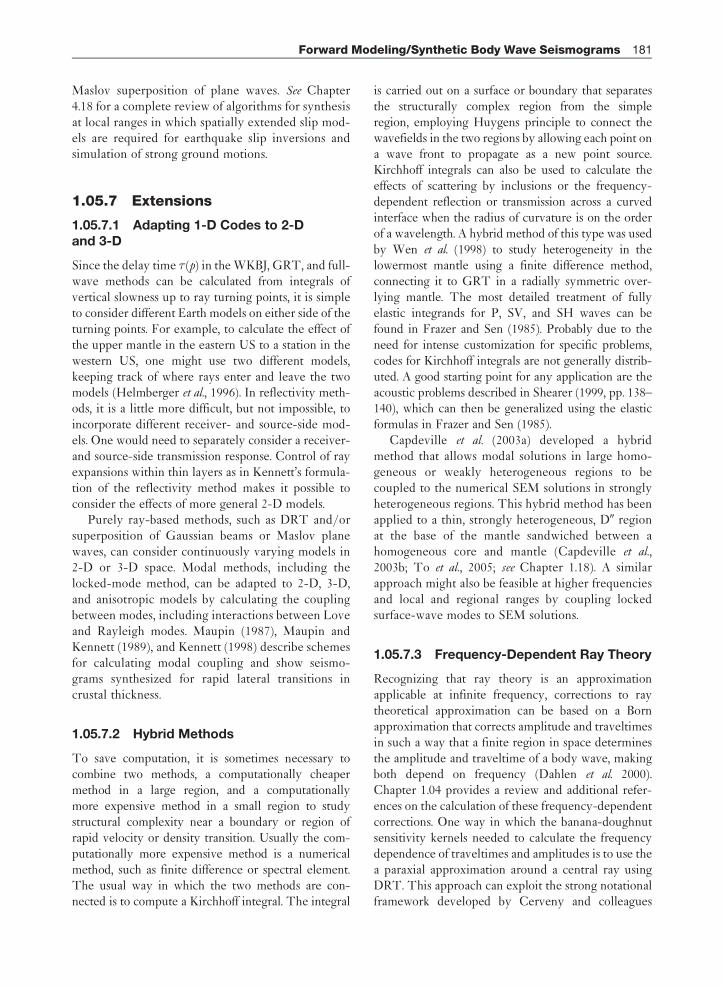
Maslov superposition of plane waves. See Chapter4.18 for a complete review of algorithms for synthesisat local ranges in which spatially extended slip mod-els are required for earthquake slip inversions andsimulation of strong ground motions.

1.05.7 Extensions

1.05.7.1 Adapting 1-D Codes to 2-Dand 3-D

Since the delay time � (p) in the WKBJ, GRT, and full-wave methods can be calculated from integrals ofvertical slowness up to ray turning points, it is simpleto consider different Earth models on either side of theturning points. For example, to calculate the effect ofthe upper mantle in the eastern US to a station in thewestern US, one might use two different models,keeping track of where rays enter and leave the twomodels (Helmberger et al., 1996). In reflectivity meth-ods, it is a little more difficult, but not impossible, toincorporate different receiver- and source-side mod-els. One would need to separately consider a receiver-and source-side transmission response. Control of rayexpansions within thin layers as in Kennett’s formula-tion of the reflectivity method makes it possible toconsider the effects of more general 2-D models.

Purely ray-based methods, such as DRT and/orsuperposition of Gaussian beams or Maslov planewaves, can consider continuously varying models in2-D or 3-D space. Modal methods, including thelocked-mode method, can be adapted to 2-D, 3-D,and anisotropic models by calculating the couplingbetween modes, including interactions between Loveand Rayleigh modes. Maupin (1987), Maupin andKennett (1989), and Kennett (1998) describe schemesfor calculating modal coupling and show seismo-grams synthesized for rapid lateral transitions incrustal thickness.

1.05.7.2 Hybrid Methods

To save computation, it is sometimes necessary tocombine two methods, a computationally cheapermethod in a large region, and a computationallymore expensive method in a small region to studystructural complexity near a boundary or region ofrapid velocity or density transition. Usually the com-putationally more expensive method is a numericalmethod, such as finite difference or spectral element.The usual way in which the two methods are con-nected is to compute a Kirchhoff integral. The integral

is carried out on a surface or boundary that separatesthe structurally complex region from the simpleregion, employing Huygens principle to connect thewavefields in the two regions by allowing each point ona wave front to propagate as a new point source.Kirchhoff integrals can also be used to calculate theeffects of scattering by inclusions or the frequency-dependent reflection or transmission across a curvedinterface when the radius of curvature is on the orderof a wavelength. A hybrid method of this type was usedby Wen et al. (1998) to study heterogeneity in thelowermost mantle using a finite difference method,connecting it to GRT in a radially symmetric over-lying mantle. The most detailed treatment of fullyelastic integrands for P, SV, and SH waves can befound in Frazer and Sen (1985). Probably due to theneed for intense customization for specific problems,codes for Kirchhoff integrals are not generally distrib-uted. A good starting point for any application are theacoustic problems described in Shearer (1999, pp. 138–140), which can then be generalized using the elasticformulas in Frazer and Sen (1985).

Capdeville et al. (2003a) developed a hybridmethod that allows modal solutions in large homo-geneous or weakly heterogeneous regions to becoupled to the numerical SEM solutions in stronglyheterogeneous regions. This hybrid method has beenapplied to a thin, strongly heterogeneous, D0 regionat the base of the mantle sandwiched between ahomogeneous core and mantle (Capdeville et al.,2003b; To et al., 2005; see Chapter 1.18). A similarapproach might also be feasible at higher frequenciesand local and regional ranges by coupling lockedsurface-wave modes to SEM solutions.

1.05.7.3 Frequency-Dependent Ray Theory

Recognizing that ray theory is an approximationapplicable at infinite frequency, corrections to raytheoretical approximation can be based on a Bornapproximation that corrects amplitude and traveltimesin such a way that a finite region in space determinesthe amplitude and traveltime of a body wave, makingboth depend on frequency (Dahlen et al. 2000).Chapter 1.04 provides a review and additional refer-ences on the calculation of these frequency-dependentcorrections. One way in which the banana-doughnutsensitivity kernels needed to calculate the frequencydependence of traveltimes and amplitudes is to use thea paraxial approximation around a central ray usingDRT. This approach can exploit the strong notationalframework developed by Cerveny and colleagues


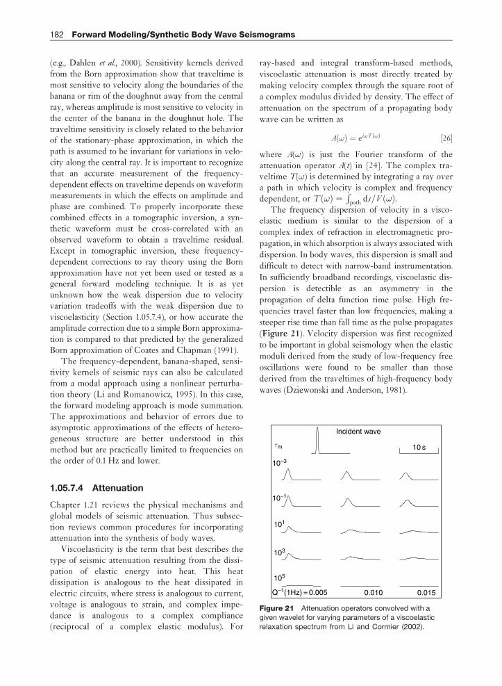
(e.g., Dahlen et al., 2000). Sensitivity kernels derivedfrom the Born approximation show that traveltime ismost sensitive to velocity along the boundaries of thebanana or rim of the doughnut away from the centralray, whereas amplitude is most sensitive to velocity inthe center of the banana in the doughnut hole. Thetraveltime sensitivity is closely related to the behaviorof the stationary-phase approximation, in which thepath is assumed to be invariant for variations in velo-city along the central ray. It is important to recognizethat an accurate measurement of the frequency-dependent effects on traveltime depends on waveformmeasurements in which the effects on amplitude andphase are combined. To properly incorporate thesecombined effects in a tomographic inversion, a syn-thetic waveform must be cross-correlated with anobserved waveform to obtain a traveltime residual.Except in tomographic inversion, these frequency-dependent corrections to ray theory using the Bornapproximation have not yet been used or tested as ageneral forward modeling technique. It is as yetunknown how the weak dispersion due to velocityvariation tradeoffs with the weak dispersion due toviscoelasticity (Section 1.05.7.4), or how accurate theamplitude correction due to a simple Born approxima-tion is compared to that predicted by the generalizedBorn approximation of Coates and Chapman (1991).

The frequency-dependent, banana-shaped, sensi-tivity kernels of seismic rays can also be calculatedfrom a modal approach using a nonlinear perturba-tion theory (Li and Romanowicz, 1995). In this case,the forward modeling approach is mode summation.The approximations and behavior of errors due toasymptotic approximations of the effects of hetero-geneous structure are better understood in thismethod but are practically limited to frequencies onthe order of 0.1 Hz and lower.

1.05.7.4 Attenuation

Chapter 1.21 reviews the physical mechanisms andglobal models of seismic attenuation. Thus subsec-tion reviews common procedures for incorporatingattenuation into the synthesis of body waves.

Viscoelasticity is the term that best describes thetype of seismic attenuation resulting from the dissi-pation of elastic energy into heat. This heatdissipation is analogous to the heat dissipated inelectric circuits, where stress is analogous to current,voltage is analogous to strain, and complex impe-dance is analogous to a complex compliance(reciprocal of a complex elastic modulus). For

ray-based and integral transform-based methods,

viscoelastic attenuation is most directly treated by

making velocity complex through the square root of

a complex modulus divided by density. The effect of

attenuation on the spectrum of a propagating body

wave can be written as

Að!Þ ¼ ei!T ð!Þ ½26�

where A(!) is just the Fourier transform of theattenuation operator A(t) in [24]. The complex tra-veltime T(!) is determined by integrating a ray overa path in which velocity is complex and frequencydependent, or T ð!Þ ¼

Rpath ds=V ð!Þ.

The frequency dispersion of velocity in a visco-elastic medium is similar to the dispersion of a

complex index of refraction in electromagnetic pro-

pagation, in which absorption is always associated with

dispersion. In body waves, this dispersion is small and

difficult to detect with narrow-band instrumentation.

In sufficiently broadband recordings, viscoelastic dis-

persion is detectible as an asymmetry in the

propagation of delta function time pulse. High fre-

quencies travel faster than low frequencies, making a

steeper rise time than fall time as the pulse propagates

(Figure 21). Velocity dispersion was first recognized

to be important in global seismology when the elastic

moduli derived from the study of low-frequency free

oscillations were found to be smaller than those

derived from the traveltimes of high-frequency body

waves (Dziewonski and Anderson, 1981).

Incident wave

10 sτm

10–3

10–1

101

103

105

0.010 0.015Q–1(1Hz) = 0.005

Figure 21 Attenuation operators convolved with a

given wavelet for varying parameters of a viscoelastic

relaxation spectrum from Li and Cormier (2002).


There is a consensus that the quality factor, Q , inthe attenuation of teleseismic body waves is nearlyindependent of or slowly varying with frequencyfrom 0.001 to 0.1 Hz, with possibly some stronger

frequency dependence beginning between 0.1 and1 Hz. For frequencies close to neither the low- orhigh-frequency corner of a relaxation spectrum

(absorption band) of constant Q , this assumptionleads to an approximate formula for complex velocityof the type

V ð!Þ ffi V ð!r Þ 1þ 1

�Q

� �ln

!

!r

� �– i

1

2Q

� �� ½27�

where V(!r) is the real velocity at a reference fre-quency. Substitution of V(!) into the ray pathintegral for complex time T(!) in [26] and invertingthe complex spectrum defines a time domainattenuation operator that is commonly termed theFutterman (1962) or Carpenter (1967) Q operator.This operator is valid in regions of the relaxationspectrum where attenuation (1/Q) is constant. It isnot valid near the corners of the true relaxationspectrum, where 1/Q decays as !�1. It is relativelysimple, however, to derive a formula for complexvelocity that is valid across the entire relaxationspectrum (e.g., Cormier and Richards, 1988). Anexample of the effect of attenuation operators con-structed with this formula is shown in Figure 21.

The width of relaxation spectra in which attenua-tion 1/Q is nearly constant or slowly varying (oftenobserved to be !1/3) is typically 5 decades in fre-quency (Anderson and Given, 1981). A problem often

not considered in modeling the effects of viscolasti-city are the limitations viscoelastic theory imposes onthe difference between the static (relaxed) elastic

modulus and the infinite frequency (unrelaxed) mod-ulus. There are limits on the band over whichviscoleastic Q can be constant given by this modulus

difference or defect. In practice, this means that anyQ inferred from a body-wave pulse width or spec-trum that has an exceptionally low value, for

example, 10 or lower, is probably the result of scat-tering rather than viscoelasticity.

Slowness or ray-based methods often treatattenuation by solving the equations of motion withreal velocities defined at the reference frequency(often chosen to be 1 Hz) and then convolving the

result with the time domain attenuation operator of[26] appropriate for each ray path. Since the units ofthis ray-path integrand are time, a parameter often

cited in the literature of teleseismic body waves is t �.Considering only the real part of [26] and assuming[27] for V(!), each frequency is exponentially atte-nuated by the factor expð –!t�Þ, where

t � ¼Z

path

1

V ð!r ÞQds ½28�

The parameter t� is found to vary relativelyslowly with range and path length of P waves inthe mantle, and is on the order of 1 s for frequenciesbetween 0.01 and 0.2 Hz in the distance range 30–90�.

Spectral methods that first compute the complexspectrum of the solution of the equation of motion(e.g., reflectivity, discrete wave number, full wave, theDSM , mode summation) can treat attenuation simplyby substituting a complex velocity and analyticallycontinuing all formulas in propagator matrices andphase factors that contain wave numbers and elasticmoduli to complex numbers. To include the dispersiveeffect of attenuation in DRT and beam summation, aFutterman-type Q operator can be convolved with thecomputed amplitude of each ray or beam calculated ina model specified at a reference frequency. Anothermore general approach would be to compute ampli-tudes by DRT at the real velocities, Re(V(!)), definedat each frequency and then multiply each spectralcomponent by an exponential scale factor

exp –!

ZIm

1

V ð!Þ

� �ds

� � –

In finite difference methods that integrate theequation of motion in the time domain, it is notpractical to handle viscoelastic attenuation by a con-volution. Instead, it is possible to design a system ofstress–strain memory functions that can be simulta-neously integrated in the time domain with theequations of motion (Robertsson et al., 1994). Usinga memory function for only three specific relaxationtimes, it is usually possible to reproduce the effects ofa relaxation spectrum of nearly constant attenuationin a frequency band of interest.

1.05.7.5 Anisotropy

Chapter 1.09 reviews the elastic anisotropy andcomputational approaches for its effects. Summarizedhere are considerations primarily related to ray- andtransform-based methods of body-wave synthesis.

Elastic anisotropy removes the degeneracy of theS-wave eigenvalue/eigenvector solutions to thewave numbers of propagating plane waves. The SH


and SV definitions defined by source and receivergeometry are no longer useful for formulatingboundary conditions needed for calculating reflec-tion and refraction. S polarization is best resolvedinto components of motion along two orthogonalquasi-S-wave eigenvectors, with motion on both theSH and SV components of motion generally consist-ing of a combination of two quasi-S waves. A pure SVpolarized wave incident on a weakly anisotropicregion excites two transmitted quasi-S waves suchthat the SH component of the transmitted wave hasthe approximate shape of the time derivative of theSV component (Silver and Chan, 1991).

A special case of anisotropic propagation is that oftransverse isotropy with a vertical axis of symmetry.In this case, the two-quasi S-waves are exactly polar-ized in the SH and SV directions defined by source–receiver geometry but with two different velocities.Transverse isotropy can be an accurate representa-tion for Earth models consisting of thin planar orradially symmetric layers, having alternating or ran-domly fluctuation velocities and layer thicknessesmuch smaller than the smallest wavelength of inter-est (Backus, 1962). Transverse isotropy can be easilyincorporated in all layered 1-D body-wave codes bymodifying the calculations of reflection–transmissioncoefficients and the � (p) function in the phase factorof WKBJ, GRT, or full-wave techniques (e.g.,Chapman, 2004).

General anisotropy breaks the symmetry uponwhich some integral transforms and spherical harmo-nic analysis are based. Body waves can propagate inand out of the sagittal plane. This makes the problemof synthesizing body waves in a generally anisotropicmodel automatically a 3-D problem. In plane-layeredmodels and Cartesian coordinates, the generalizedwave number superposition leads to reflectivity for-mulations that require integration over twohorizontal wave numbers to invert wave numbertransforms to the spatial domain (Fryer and Frazer,1984, 1987). Similarly, the WKBJ/Maslov methodscan be generalized by integrals over two horizontalslownesses (Garmany, 1989; Chapman, 2001). Someapproximations for weak general anisotropy andexpansion of the phase near its stationary point canbe employed to simplify the problem to integrationover a single wave number corresponding to wavespropagating in and near the saggital plane. Forseismograms synthesized by DRT or Gaussianbeam summation, the kinematic system neededfor ray trajectory and traveltimes is easilyextended to the case of general anisotropy, where

an eignevector–eigenvalue problem for the wavetypes is solved for each spatial or time incrementused in numerical integration. A system for dynamicquantities corresponding to the P and Q matrices canbe formulated for summation of Gaussian beams(Hanyga, 1986), but a more tractable approach is totake difference derivatives of ray positions and slow-nesses (Gajewski and Psencik, 1987) to determinegeometric spreading and wave front curvature.

1.05.7.6 Scattering

Chapter 1.20 reviews seismic scattering. A few funda-mental effects important to consider in the synthesisof body waves are reviewed here, some of which arecomputationally simple to include.

Single scattering by small-scale heterogeneity canbe incorporated by a Born approximation (e.g.,Chapman, 2004, chapter 10). The Born approxima-tion effectively treats small perturbations in velocityand density from a background medium as seismicsources by moving terms due to the difference inperturbed velocity from the background velocity tothe source side of the wave equation. The strength ofthese scattering sources that re-radiate energy areproportional to the energy of the wave incident onthe heterogeneity and the size of its perturbations.For wavelengths much greater than the heterogene-ity, each heterogeneity can be treated by a point-source representation similar to the moment-ratetensor representation of earthquake sources (Wuand Aki, 1985). The effects of many small-scale het-erogeneities can be obtained by summing theradiated body waves of each small scatterer. TheGreen’s function solutions of the equations of motionmust be known from the source to the position ofeach scatterer and from the scatterer to the receiver.These Green’s functions can be calculated by any ofthe methods described in Section 1.05.4. The volumeof the region of scatterers contributing to a specifictime window surrounding a body wave is the banana-shaped region surrounding a least-time ray describedin Section 1.05.7.3. An example of this approach is thesynthesis of the precursor coda of PKIKP from scat-terers near the core–mantle boundary (Cormier,1999).

Forward scattering in the direction close to thedirection of the least-time ray can affect the pulseshape of broadband body waves. A finite frequencyband of observation can blur the effects of manyscatterers, whose arrivals can occur over time spa-cings much shorter than the shortest period in the


pass band of observation. This broadening and multi-pathing can be mistaken for the effects of viscoelasticattenuation. Unlike viscoelastic attenuation, whereenergy is lost to heat, scattering attenuation simplyredistributes high-frequency energy in time andspace out of a finite time window surrounding thepulse observed at a particular location. One recentapproximate method of including this effect is thetheory of dynamic composite elastic moduli(DYCEM) of Kaelin and Johnson (1998). This tech-nique can be formulated in terms of a complex wavenumber, allowing it to be treated in much the sameway as complex velocities in viscoelasticity (e.g.,Cormier and Li, 2002).

1.05.8 Conclusions

Most of the algorithms for synthesizing body wavesin radially symmetric (1-D) structure have been suc-cessfully tested and verified against each other (e.g.,Choy et al., 1980; Figure 12). Factors to consider inchoosing an algorithm include the accuracy in arequired frequency band and distance range, thewidth of the time window and number and types ofseismic phases, speed of computation, the complete-ness of documentation, and the existence andaccessibility of software.

The frequency band of calculation is probably theforemost important factor. If working in the fre-quency band less than several one-tenths of a hertz,then modal summation or the DSM are good choicesbecause they easily include all possible body waves,surface waves, and frequency-dependent interactionswith discontinuities in an arbitrarily wide time win-dow at an acceptable computational cost on a singleworkstation. Using a perturbation approach, they canalso handle weak lateral heterogeneity (several per-cent perturbation in velocity and density) with littleadditional computational overhead. At higher fre-quencies, reflectivity/GRT or locked-modeapproaches in thin homogeneous layers or asympto-tically approximate ray-based methods (WKBJ/fullwave/Maslov/DRT and Gaussian beams) in homo-geneous layers are efficient and produce identicalresults if carefully used.

In either low- or high-frequency bands, the mostimportant limitations of each algorithm are related toits accurate reproduction of the waveform effects ofthe broad spatial spectrum of Earth structure. In allalgorithms, it is important to consider the effects ofneglecting small-scale structure on the order of a

wavelength or smaller. In high-frequency algorithms,limitations are related to either the validity of theEFA, the physicality of thin-layer representations, orthe validity of asymptotic approximations of wavefunctions in layers having continuous and large spa-tial gradients. Understanding these limitations is alsokey to the problems of separating the effects of ani-sotropy from heterogeneity and viscoelasticity fromscattering.

Computational hardware now makes it possible toroutinely model seismic waveforms to invert for bothradially symmetric (1-D) Earth structure and simplepoint-source representations of earthquake faulting.Recent advances in digital recording and networktelemetry have now made these inversions possiblein near real-time. The remaining advance needed tofully exploit the real-time capabilities of 1-D model-ing lies in making user-friendly software interfaces.

Three-dimensional modeling is still strongly lim-ited by current computational hardware. Ray-based3-D modeling is feasible on single workstations insmooth models having a relatively large ratio of scalelength of heterogeneity to wavelength and for rela-tively mild velocity and density perturbations (lessthan several percent). Similarly, perturbationapproaches based on mode summation or the DSMcan be performed with modest computational over-head for relatively weak velocity perturbations(several percent) and at large scale lengths (thou-sands of kilometers). Investigation of effects of verysmall-scale heterogeneity (10 km or less) at high fre-quencies (>1 Hz) can be done in 3-D but is currentlyonly practical for ranges on the order of hundreds ofwavelengths using clusters of processors. An effort totest and verify 3-D modeling algorithms against eachother has just begun in the last several years (Igelet al., 2000).

Acknowledgments

The author thanks the National Science Foundationfor continued support on problem in wave propaga-tion and Earth structure, most recently under grantEAR 02-29586.

References

Abo-Zena A (1979) Dispersion function computations for unlim-ited frequency values. Geophysical Journal of the RoyalAstronomical Society 58: 91–105.


Aki K and Richards PG (1980) Quantitative Seismology: Theoryand Methods. San Francisco, CA: W.H. Freeman.

Aki K and Richards PG (2002) Quantitative Seismology, 2ndedn. Sausalito, CA: University Science Books.

Anderson DL and Given JW (1982) Absorption band Q model forthe Earth. Journal of Geophysical Research 87: 3893–3904.

Baag C and Langston CA (1985) Shear-coupled PL.Geophysical Journal of the Royal Astronomical Society80: 363–385.

Backus GE (1962) Long-wave elastic anisotropy produced byhorizontal layering. Journal of Geophysical Research67: 4427–4440.

Ben-Menahem A and Beydoun WB (1985) Range of validity ofseismic ray and beam methods in general inhomogeneousmedia, Part I: General theory. Geophysical Journal of theRoyal Astronomical Society 82: 207–234.

Bouchon M and Aki K (1977) Discrete wave-number represen-tation of seismic wave source fields. Bulletin of theSeismological Society of America 67: 259–277.

Bouchon M (1979) Discrete wave number representation ofelastic wave fields in three-space dimensions. Journal ofGeophysical Research 84: 3609–3614.

Breger L and Romanowicz B (1998) Three dimensional structureat the base of the mantle beneath the central Pacific.Science 382: 244–248.

Brune JN (1970) Tectonic stress and the spectra of seismicshear waves from earthquakes. Journal of GeophysicalResearch 75: 4997–5009.

Bullen KE and Bolt BA (1985) Introduction to the Theory ofSeismology, pp. 499. Cambridge, UK: Cambridge UniversityPress.

Burdick LJ and Helmberger DV (1978) The upper mantle Pvelocity stucture of the Western United States. Journal ofGeophysical Research 83: 1699–1712.

Burdick LJ and Orcutt JA (1979) A comparison of the general-ized ray and reflectivity methods of waveform synthesis.Geophysical Journal of the Royal Astronomical Society58: 261–278.

Capdeville Y, Chaljub E, Vilotte JP, and Montagner JP (2003a)Coupling the spectral element method with a modal solutionfor elastic wave propagation in global Earth models.Geophysical Journal International 153: 34–66.

Capdeville Y, Romanowicz B, and To A (2003b) Couplingspectral elements and modes in a spherical Earth: Anextension to the ‘sandwich’ case. Geophysical JournalInternational 154: 44–57.

Carpenter EW (1967) Teleseismic signal calculated for under-ground, underwater, and atmospheric explosions.Geophysics 32: 17–32.

Cerveny V and Ravindra R (1971) Theory of Seismic HeadWaves. Toronto, ON: University of Toronto Press.

Cerveny V (1985) The application of ray tracing to the numericalmodelin of the seismic wave field in complex structures.In: Helbig K and Treitel S (eds.) Seismic Shear Waves:Handbook of Geophysical Exploration, Section I: SeismicExploration, vol. 15A, pp. 1–124. London: GeophysicalPress.

Cerveny V, Pleinerova J, Klimes L, and Psencık I (1987) Highfrequency radiation from earthquake sources in laterallyvarying structures. Geophysical Journal of the RoyalAstronomical Society 88: 43–80.

Cerveny V (2001) Seismic Ray Theory. New York: CambridgeUniversity Press.

Chapman CH (1973) The Earth flattening transformation in bodywave theory. Geophysical Journal of the Royal AstronomicalSociety 35: 55–70.

Chapman CH (1978) A new method for computing syntheticseismograms. Geophysical Journal of the RoyalAstronomical Society 54: 481–518.

Chapman CH and Drummond R (1982) Body-wave seismo-grams in inhomogeneous media using Maslov asymptotictheory. Bulletin of the Seismological Society of America72: S277–S317.

Chapman CH, Chu J-Y, and Lyness DG (1988) The WKBJseismogram algorithm. In: Doornbos DJ (ed.) SeismologicalAlgorithms, pp. 47–74. London: Academic Press.

Chapman CH (2004) Fundamentals of Seismic WavePropagation. Cambridge, UK: Cambridge University Press.

Choy GL and Richards PG (1975) Pulse distortion and Hilberttransformation in multiply reflected and refracted bodywaves. Bulletin of the Seismological Society of America65: 55–70.

Choy GL, Cormier VF, Kind R, Muller G, and Richards PG (1980)A comparison of synthetic seismograms of phases gener-ated by the full wave theory and by the reflectivity method.Geophysical Journal of the Royal Astronomical Society61: 21–39.

Choy GL and Cormier VF (1983) The structure of the inner coreinferred from short-period and broad-band GDSN data.Geophysical Journal of the Royal Astronomical Society72: 1–21.

Choy GL and Engdahl ER (1987) Analysis of broadband seis-mograms from selected IASPEI events. Physics of Earth andPlanetary Interiors 447: 80–92.

Choy GL and Boatwright J (2004) Radiated energy and therupture process of the Denali Fault earthquake sequence of2002 from broadband teleseismic body waves. Bulletin ofthe Seismological Society of America 94: S269–S277.

Cline AK (1874) Six subprograms for curve fitting usingsplines under tension. Communications of the ACM17: 220–223.

Coates RT and Chapman CH (1991) Generalized Born scatter-ing of elastic waves in 3D media. Geophysical JournalInternational 107: 231–263.

Cormier VF (1999) Anisotropy of heterogeneity scale lenths inthe lowermost mantle from PKIKP precursors. GeophysicalJournal International 136: 373–384.

Cormier VF (2000) D’’ as a transition in the heterogeneity spec-trum of the lowermost mantle. Journal of GeohysicalResearch 105: 16193–16205.

Cormier VF and Choy GL (1981) Theoretical body wave inter-actions with upper mantle structure. Journal of GeophysicalResearch 86: 1673–1678.

Cormier VF and Li X (2002) Frequency dependent attenuation inthe inner core: Part II. A scattering and fabric interpretation.Journal of Geophysical Research 107(B12): 2362(doi:10.1029/2002JB1796).

Cormier VF, Mandal B, and Harvey D (1991) Incorporation ofvelocity gradients in the synthesis of complete seismogramsby the locked mode method. Bulletin of the SeismologicalSociety of America 81: 897–930.

Cormier VF and Richards PG (1977) Full wave theory applied toa discontinuous velocity increase: The inner core boundary.Journal of Geophysics 43: 3–31.

Cormier VF and Richards PG (1988) Spectral synthesis of bodywaves in Earth models specified by vertically varying layers.In: Doornbos D (ed.) Seismological Algorithms, pp. 3–45.London: Academic Press.

Crotwell HP, Owens TJ, and Ritsema J (1999) The TauP Toolkit:Flexible seismic travel-time and raypath utilities.Seismological Research Letters 70: 154–170.

Cummins PR, Geller RJ, Hatori T, and Takeuchi N (1994a)DSM complete synthetic seismograms: SH, sphericallysymmetric, case. Geophysical Research Letters21: 533–536.

Cummins PR, Geller RJ, and Takeuchi N (1994b) DSM completesynthetic seismograms: P-SV, spherically symmetric, case.Geophysical Research Letters 21: 1663–1666.


Dahlen FA (1987) Multiplet coupling and the calculation of syn-thetic long-period seismograms. Geophysical Journal of theRoyal Astronomical Society 91: 241–254.

Dahlen FA and Tromp J (1998) Theoretical Global Seismology,P. 944. Princeton, NJ: Princeton University.

Dahlen FA, Hung S-H, and Nolet G (2000) Frechet kernels forfinite-frequency traveltimes-I. Theory. Geophysical JournalInternational 141: 157–174.

Davis JP and Henson IH (1993) Users Guide to Xgbm: An X-Windows System to Compute Gaussian Beam SyntheticSeismograms, Rept TGAL-93-02. Alexandria, VA: Teledyne-Geotech.

Doornbos DJ (ed.) (1988) Seismological Algorithms:Computational Methods and Computer Programs, P. 469.New York: Academic Press.

Dziewonski AM, Chou T-A, and Woodhouse JH (1981)Determination of earthquake source parameters fromwaveform data for studies of global and regional seismicity.Journal of Geophysical Research 86: 2825–2852.

Dziewonski AM and Anderson DL (1981) Prelminary referenceEarth model. Physics of the Earth and Planetary Interiors25: 297–356.

Felsen LB (1984) Geometrical theory of diffraction,evanescent waves, complex rays and Gaussian beams.Geophysical Journal of the Royal Astronomical Society79: 77–88.

Fornberg B (1998) A Practical Guide to PseudospectralMethods. Cambridge, UK: Cambridge University Press.

Frankel A and Clayton RW (1986) Finite-difference simulationsof seismic scattering: Implications for the propagation ofshort-period seismic waves in the crust and models ofcrustal heterogeneity. Journal of Geophysical Research91: 6465–6489.

Frazer LN and Gettrust JF (1984) On a generalization of Filon’smethod and the computation of the oscillatory integrals ofseismology. Geophsical Journal of the Royal AstronomicalSociety 76: 461–481.

Frazer LN and Sen M (1985) Kirchhoff–Helmholtz reflectionseismograms in a laterally variable multi-layered elasticmedium. Part I. Theory. Geophysical Journal of the RoyalAstronomical Society 80: 121–147.

Fryer GJ and Frazer LN (1984) Seismic waves in stratified ani-sotropic media. Geophysical Journal of the RoyalAstronomical Society 78: 691–710.

Fryer GJ and Frazer LN (1987) Seismic waves in stratified ani-sotropic media – II. Elastodynamic eigensolutions for someanisotropic systems. Geophysical Journal of the RoyalAstronomical Society 91: 73–101.

Fuchs K and Muller G (1971) Computation of synthetic seis-mograms with the reflectivity method and comparison withobservations. Geophysical Journal of the Royal AstronomicalSociety 23(4): 417–433.

Furumura T, Kennett BLN, and Furumura M (1998) Seismicwavefield calculation for laterally heterogeneous sphericalEarth models using the pseudospectral method.Geophysical Journal International 135: 845–860.

Futterman WI (1962) Dispersive body waves. Journal ofGeophysical Research 67: 5279–5291.

Gajewski D and Psencik I (1987) Computation of high-frequencyseismic wavefields in 3-D laterally inhomogeneous aniso-tropic media. Geophysical Journal of the Royal AsronomicalSociety 91: 383–411.

Garmany J (1989) A student’s graden of anisotropy. AnnualReview of Earth and Planetary Sciences 17: 285–308.

Geller RJ and Ohminato T (1994) Computation of syntheticseismograms and their partial derivatives for heterogeneousmedia with arbitrary natural boundary conditions using thedirect solution method (DSM). Geophysical JournalInternational 116: 421–446.

Gilbert F and Backus GE (1966) Propagator matrices inelastic wave and vibration problems. Geophysics31: 326–332.

Grand SP, van der Hilst RD, and Widiyantoro S (1997) Globalseismic tomography; a snapshot of convection in the Earth.GSA Today 7: 1–7.

Gu YJ, Dziewonski AM, Su W-J, and Ekstrom G (2001) Modelsof the mantle shear velocity and discontinuities in the patternof lateral heterogeneities. Journal of Geophysical Research106: 11169–11199.

Hanyga H (1986) Gaussian beams in anisotropic elastic media.Geophysical Journal of the Royal Astronomical Society85: 473–503.

Harvey DJ (1981) Seismogram synthesis using normal modesuperposition: The locked mode approximation.Geophysical Journal of the Royal Astronomical Society66: 37–69.

Harvey D and Choy GL (1982) Broadband deconvolution ofGDSN data. Geophysical Journal of the Royal AstronomicalSociety 69: 659–668.

Hartzell S, Harmsen S, Frankel A, and Larsen S (1999)Calculation of broadband time histories of ground motion:Comparison of methods and validation using strong-ground motion from the 1994 Northridge earthquake.Bulletin of the Seismological Society of America89: 1484–1504.

Helmberger DV (1974) Generalized ray theory for shear dislo-cations. Bulletin of the Seismological Society of America64: 45–64.

Helmberger DV and Engen, GR (1974) Upper mantle shearstructure. Journal of Geophysical Research 79: 4017–4028.

Helmberger DV and Harkrider D (1978) Modeling earthquakeswith generalized ray theory. In: Miklowitz J andAchenbach JD (eds.) Modern Problems in Elastic WavePropagation. New York: Wiley.

Helmberger DV, Zhao LS, and Garnero EJ (1996) Constructionof synthetics for 2D structures, core phases. In: Boschi E andEkstrom G (eds.) Proceedings of International School of SolidEarth Geophysics: Seismic Modeling of the Earth’s Structure,pp. 183–222. Bologna, Italy: Societa Italiana di Fisica.

Honda R and Yomogida K (2003) Static and dynamic displace-ment near a fault with the discrete wavenumber method.Physics of the Earth and Planetary Interiors 137: 107–127.

Holliger K, Levander A, and Goff JA (1993) Stochastic modelingof the reflective lower crust: Petrophysical and geologicalevidence from the Ivrea Zone (northern Italy). Journal ofGeophysical Research 98: 11967–11980.

Igel H (1999) Modeling wave propagation in 3-D spherical sec-tions by the Chebyshev spectral method. GeophysicalJournal International 136: 559–567.

Igel H, Takeuchi N, Geller RJ, et al. (2000) The COSY Project:Verification of global seismic modeling algorithms. Physicsof the Earth and Planetary Interiors 119: 3–23.

Imhof MG and Toksoz MN (2000) Multiple multipole expansionsfor elastic scattering. Journal of the Acoustic Society ofAmerica 100: 2969–2979.

Jeffreys H (1936) The structure of the Earth down to the 20discontinuity. Monthly Notices of the Royal AstronomicalSociety Geophysical Supplement 3: 401–422.

Kaelin B and Johnson LR (1998) Dynamic composite elasticmedium theory. Part II. Three-dimensional media. Journal ofApplied Physics 84: 5488–5468.

Karato S-I (1993) Importance of anelasticity in the interpretationof seismic tomography. Geophysical Research Letters20: 1623–1626.

Keith M and Crampin S (1977) Seismic body waves in aniso-tropic media: Reflection and refraction at a plane interface.Geophysical Journal of the Royal Astronomical Society49: 181–208.


Kind R (1985) The reflectivity method for different source andreceiver structures and comparison with GRF data. Journalof Geophysics 58: 146–152.

Kennett BLN (1983) Seismic Wave Propagation in StratifiedMedia. New York: Cambridge University Press.

Kennett BLN (1998) Guided-waves in three-dimensional struc-tures. Geophysical Journal International 133: 159–174.

Kennett BLN (2001) The Seismic Wavefield, vols. I and II. NewYork: Cambridge University Press.

Komatitsch D and Vilotte J-P (1998) The spectral elementmethod: An efficient tool to simulate the seismic response of2D and 3D geological structures. Bulletin of theSeismological Society of America 88: 368–392.

Komatitsch D and Tromp J (1999) Introduction to the spectral-element method for 3-D seismic wave propagation.Geophysical Journal International 139: 806–822.

Komatitsch D and Tromp J (2002) Spectral-element simulationsof global seismic wave propagation-II. 3-D models, oceans,rotation, and self gravitation. Geophysical JournalInternational 149: 390–412.

Korneev VA and Johnson LR (1993) Scattering of elastic wavesby a spherical inclusion – I. Theory and numerical results.Geophysical Journal International 115: 230–250.

Kosloff D and Kessler D (1990) Seismic Numerical Modeling:Oceanographic and Geophysical Tomography, pp. 251–312.Amsterdam: Elsevier Science Publishers.

Langston CA and Helmberger DV (1975) A procedure for mod-eling dislocation sources. Geophysical Journal 42: 112–130.

Lapwood ER and Usami T (1981) Free Oscillations of the Earth.Cambridge, UK: Cambridge University Press.

Larsen S and Schultz CA (1995) ELAS3D: 2D/3D elastic finitedifference propagation code, Technical Report No. UCRL-MA-121792, p. 19 Livermore, CA: Lawrence LivermoreNational Laboratory.

Li X-D and Tanimoto T (1993) Waveforms of long period bodywaves in a slightly aspherical earth model. GeophysicalJournal International 112: 92–102.

Li X-D and Romanowicz B (1995) Comparison of global wave-form inversions with and without considering cross branchcoupling. Geophysical Journal International 121: 695–709.

Li X and Cormier VF (2002) Frequency dependent attenuation inthe inner core: Part I. A viscoelastic interpretation. Journal ofGeophysical Research 107, doi:10.1029/2002JB001795.

Masters G, Laske G, Bolton H, and Dziewonski A (2000) Therelative behavior of shear velocity, bulk sound speed, andcompressional velocity in the mantle: Implications for che-mical and thermal structure. In: Karato S, Forte AM,Liebermann RC, Masters G, and Stixrude L (eds.) AGUMonograph 117: Earth’s Deep Interior, pp. 63–86.Washington, DC: AGU.

Maupin V and Kennett BLN (1987) On the use of truncatedmodel expansion in laterally varying media. GeophysicalJournal of the Royal Astronomical Society 91: 837–851.

Maupin V (1989) Numerical modeling of Lg wave propagationacross the North Sea Central Graben. Geophysical JournalInternational 99: 273–283.

Menke W and Richards PG (1980) Crust–mantle whisperinggallery phases: A deterministic model of teleseismic Pn wavepropagation. Journal of Geophysical Research85: 5416–5422.

Menke W (2005) Case studies of seismic tomography andearthquake location in a regional context. In: Levander A andNolet G (eds.) Geophysical Monograph Series 157: SeismicEarth: Array Analysis of Broadband Seismograms, pp. 7–36.Washington, DC: American Geophysical Union.

Muller G (1973) Amplitude studies of core phases. Journal ofGeophysical Research 78: 3469–3490.

Muller G (1977) Earth-flattening approximation for body wavesderived from geometric ray theory; improvements,

corrections and range of applicability. Journal of Geophysics42: 429–436.

Muller G (1985) The reflectivity method: A tutorial. Journal ofGeophysics 58: 153–174.

Ni SD, Ding X, and Helmberger DV (2000) Constructing syn-thetics from deep Earth tomographic models. GeophysicalJournal International 140: 71–82.

Olsen KB (2000) Site amplification in the Los Angeles basin fromthree-dimensional modeling of ground motion. Bulletin of theSeismological Society of America 90: S77–S94.

Rial JA and Cormier VF (1980) Seismic waves at theepicenter’s antipode. Journal of Geophysical Research85: 2661–2668.

Richards PG (1973) Calculation of body waves, for caustics andtunnelling in core phases. Geophysical Journal of the RoyalAstronomical Society 35: 243–264.

Richards PG and Frasier CW (1976) Scattering of elastic wavesfrom depth dependent inhomogeneities. Geophysics41: 441–458.

Ritsema J and van Heijst HJ (2000) Seismic imaging of struc-tural heterogeneity in Earth’s mantle: Evidence for large-scale mantle flow. Science Progress 83: 243–259.

Robertsson JOA, Blanch JO, and Symes WW (1994)Viscoelastic finite-difference modeling. Geophysics59: 1444–1456.

Rost S and Thomas C (2002) Array seismology: Methods andapplications. Reviews of Geophysics 40, doi:10.1029/2000RG000100.

Sambridge M and Gudmundsson O (1998) Tomography withirregular cells. Journal of Geophysical Research103: 773–781.

Shearer PM (1999) Introduction to Seismology. Cambridge, UK:Cambridge University Press.

Spudich P and Frazer LN (1984) Use of ray theory to calculatehigh-frequency radiation from earthquake sourceshaving spatially variable rupture velocity and stress drop.Bulletin of the Seismological Society of America74: 2061–2082.

Su W-J and Dziewonski AM (1997) Simultaneous inversions for3-D variations in shear and bulk velocity in the mantle.Physics of the Earth and Planetary Interiors 100: 135–156.

Takeuchi N, Geller RJ, and Cummins PR (2000) Complete syn-thetic seismograms for 3-D heterogeneous Earth modelscomputed using modified DSM operators and their applic-ability to inversion for Earth structure. Physics of the Earthand Planetary Interiors 119: 25–36.

To A, Romanowicz B, Capdeville Y, and Takeuchi N (2005) 3Deffects of sharp boundaries at the borders of the African andPacific superplumes: Observation and modeling. Earth andPlanetary Science Letters 233: 137–153.

Trampert J, Vacher P, and Vlar N (2001) Sensitivities of seismicvelocities to temperature, pressure and composition in thelower mantle. Physics of the Earth and Planetary Interiors124: 255–267.

Virieux J (1985) SH-wave propagation in heterogeneous media:Velocity stress finite difference method. Geophysics49: 1933–1957.

Virieux J (1986) P–SV wave propagation in heterogeneousmedia: Velocity–stress finite-difference method. Geophysics51: 889–901.

Ward SN (1978) Long period reflected and converted uppermantle phases. Bulletin of the Seismological Society ofAmerica 68: 133–153.

Wen L and Helmberger DV (1998) A two-dimensional P–SVhybrid method and its application to modeling localizedstructures near the core–mantle boundary. Journal ofGeophysical Research 103: 17901–17918.

Wu RS and Aki K (1985) Scattering characteristics of waves byan elastic heterogeneity. Geophysics 50: 582–595.


Zhao Y and Anderson DL (1994) Mineral physics constraints onthe chemical composition of Earth’s lower mantle. Physics ofthe Earth and Planetary Interiors 85: 273–292.

Relevant Websites

http://www.geodynamics.org – CIG, Computational

Infrastructure for Geodynamics

http://www.eas.slu.edu – Computer Programs in

Seismology, Department of Earth & Atmospheric

Sciences, Saint Louis University.

http://www.geophysik.uni-muenchen.de – Geophysics,

Department of Earth and Environmental Sciences,

Ludwiq-Maximilians, University.

http://www.iris.edu – IRIS, Incorporated Research

Institutions for Seismology.

http://www.ngdc.noaa.gov – NGDC Seismological

Algorithms, USDOC/NOAA/NESDIS/National

Geophysical Data Center (NGDC) Home Page.

http://www.orfeus-eu.org – Seismological Software

Library, ORFEUS.

http://www.rses.anu.edu.au – Perspective Images of

Slab Models by Oli Gudmundsson and Malcolm

Sambridge, The RUM, ANU Research School of Earth

Sciences.

http://sw3d.mff.cuni.cz – Seismic Waves in Complex 3-D

Structures (SW3D), Charles University of Prague.

http://www.geom.uiuc.edu – The Geometry Center.


1.05 Theory and Observations – Forward Modeling/Synthetic Body … · 1.05 Theory and...

Documents

Transcript of 1.05 Theory and Observations – Forward Modeling/Synthetic Body … · 1.05 Theory and...