103 PPT Bekker
40
Risk Management of Investment Guarantees in Life Insurance Kobus Bekker * & Jan Dhaene # * ABSA Life, South Africa # KU Leuven, Belgium
description
G
Transcript of 103 PPT Bekker

Risk Management of
Investment Guarantees in
Life Insurance
Kobus Bekker* & Jan Dhaene#
* ABSA Life, South Africa# KU Leuven, Belgium
Outline
• Investment Guarantees
• Risk management considerations
• Conditional lower bound approximation
• Asset-based charges
• Hedging
Slide 2

Investment Guarantees
Slide 3
Tax Deferred annuities served as tax-deferred vehicle with pure risk benefits, e.g. endowment with fixed benefits.
Investment Upside Policyholders became more aware of investment potential and demanded more investment upside exposure and investment choice.
Marketability Guarantees were offered to transfer downside risk back to insurers and to improve the marketability of VA / UL products
Mispricing Guarantees that were considered to be far OTM were offered at very low and sometimes without charges in early days.
Risk management considerations not integral to pricing and product development.
Brief background to VA & UL business

Investment Guarantees
Slide 4
GMDB (1980) Guarantees a minimum amount payable on death
GMIB / GAO (1996) Guarantees a minimum rate of interest at conversion of a lump sum to an immediate annuity
GMMB / GMAB(2002)
Guarantees a minimum amount payable at maturity or at fixed intervals over the policy term
GMWB (2002) Guarantees withdrawals to at least the value of the original premium over a specified term
GLWB (2004) Guarantees a percentage withdrawal over the remaininglifetime of the policyholder
Types of Investment Guarantees

• VA sales positively correlated, while fixed annuity sales negatively correlated
• Policyholders buy VAs at market highs and fixed annuities at market lows
Investment Guarantees
Slide 5
Policyholder preferences and the market
Slide 5
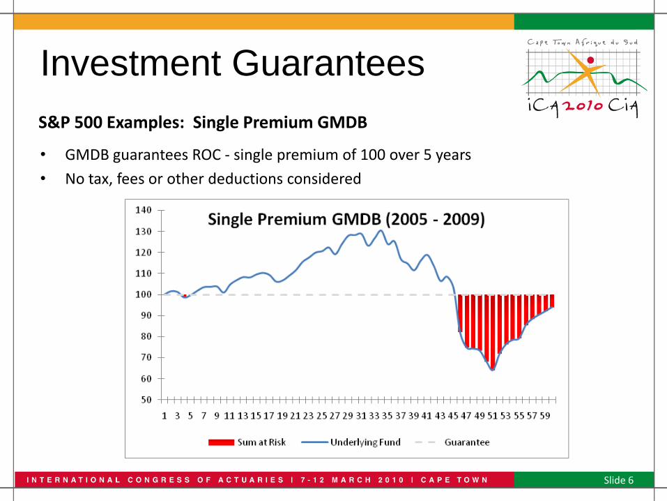
• GMDB guarantees ROC - single premium of 100 over 5 years
• No tax, fees or other deductions considered
Investment Guarantees
Slide 6
S&P 500 Examples: Single Premium GMDB
Slide 6

• Guarantee very sensitive to initial value of the underlying fund
• Phasing-in of single premiums can mitigate risk
Investment Guarantees
Slide 7
S&P 500 Examples: Single Premium GMDB
Slide 7

• One year difference (one year earlier) can lead to drastically different results!
Investment Guarantees
Slide 8
S&P 500 Examples: Single Premium GMDB
Slide 8
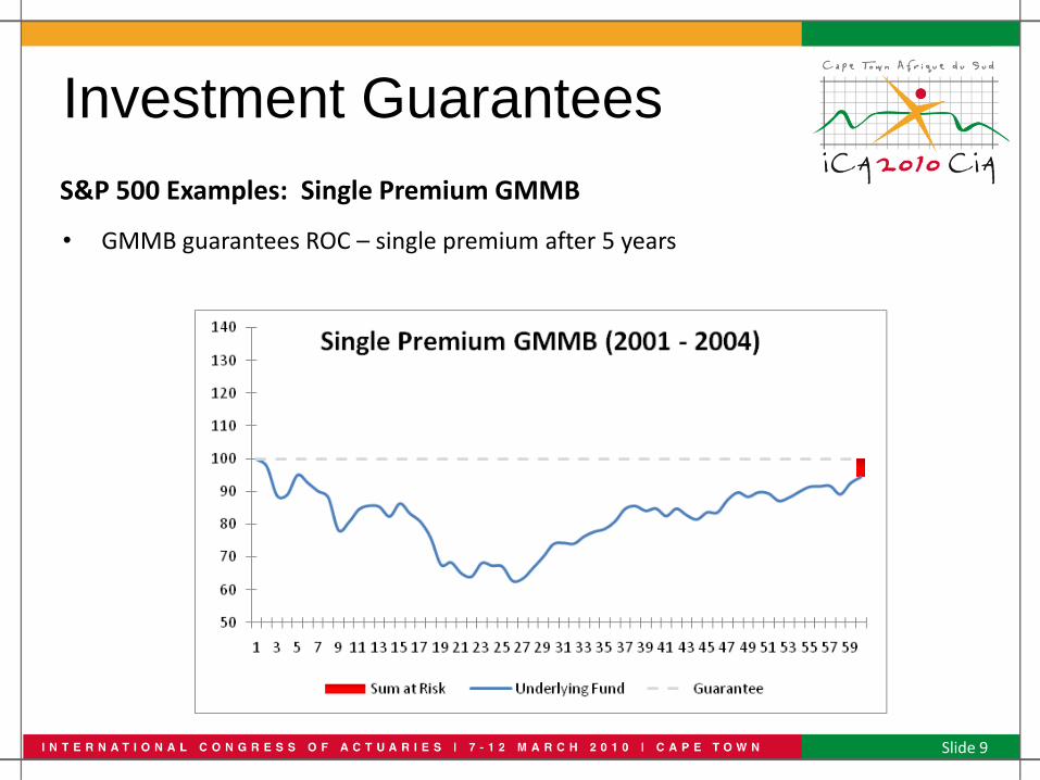
• GMMB guarantees ROC – single premium after 5 years
Investment Guarantees
Slide 9
S&P 500 Examples: Single Premium GMMB
Slide 9

• GMDB guarantees ROC – regular premium of 5 over 5 years
• Dollar cost-averaging significantly reduces risk (cf. phasing-in of single premium)
Investment Guarantees
Slide 10
S&P 500 Examples: Regular Premium GMDB
Slide 10

• Unfortunately, crises do happen (quite regularly!)
• Risk mitigating strategies such as hedging necessary
Investment Guarantees
Slide 11
S&P 500 Examples: Regular Premium GMDB
Slide 11

• GMWB guarantees 20% withdrawals for annually for 5 years
• Absorbing barrier at zero
Investment Guarantees
Slide 12
S&P 500 Examples: GMWB
Slide 12

Risk Management
Considerations
Slide 13
Dependency Guarantees of individual policies largely dependent, i.e. should one guarantee bite, others will probably follow
Combined Market Real world independence not necessarily maintained under change of measure from physical probability P to equivalent martingale measure Q.
Even more complex issue if combined market consist of policyholder preferences, e.g. GMWB
Initial Strain Typically, guarantee charges are asset-based, i.e. the initial value needed to set up a replicating portfolio is recouped over time.
Complexity Nested runs needed to determine value of guarantee inscenario-based valuation
Some key challenges

Risk Management
Considerations
Slide 14
ESG valuation of investment guarantees
• Investment guarantee value needs to be solved via nested simulation runs based on the economic parameters of each main run.

Risk Management
Considerations
Slide 15
ESG valuation of investment guarantees
• Instead, an approximation (CLB) can be used for interim valuations and economic capital scenario testing.
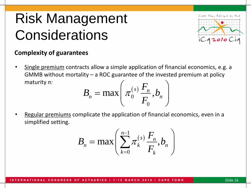
• Single premium contracts allow a simple application of financial economics, e.g. a GMMB without mortality – a ROC guarantee of the invested premium at policy maturity n:
• Regular premiums complicate the application of financial economics, even in a simplified setting.
Risk Management
Considerations
Slide 16
Complexity of guarantees
0
0
max ,s n
n n
FB b
F
1
0
max ,n
s nn k n
k k
FB b
F

Risk Management
Considerations
Slide 17
Embedded arithmetic Asian options
No analytical solution Several approximations available, e.g. based on geometric Asian options, but no analytical solutions –even in simplified settings.
Conditional lower bound
Dhaene et al. (2002) derived accurate bounds for arithmetic Asian options in Black-Scholes-Merton setting.
The conditional lower bound proved exceptionally accurate and will be used as an approximation.
Further outline Conditional lower bound (CLB) is derived for simple GMMB and GMDB products.
Asset-based charges are determined for these products.
CLB will be used for possible hedging strategy.
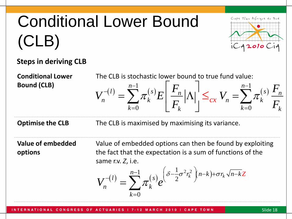
Conditional LowerBound (CLB)
The CLB is stochastic lower bound to true fund value:
Optimise the CLB The CLB is maximised by maximising its variance.
Value of embedded options
Value of embedded options can then be found by exploitingthe fact that the expectation is a sum of functions of the same r.v. Z, i.e.
Conditional Lower Bound
(CLB)
Slide 18
Steps in deriving CLB
2 211
2
0
k kn r n k r n k
l s
n k
k
Z
V e
1 1
0 0
n nl s sn n
n k n k
k kk k
cx
F FV E V
F F

Conditional Lower Bound
(CLB)
Slide 19
Comonotonicity as a tool
• One condition for a random vector X to be comonotonic is if there exist a random variable Z and non-decreasing functions fi such that:
• In the case of a comonotonic sum Sc, we have that the stop-loss premiums of the sum is equal to the sum of the comonotonic components Xi:
where
1 2, ,...,d nX f Z f Z f Z
1
nc
i i
i
E S d E X d
1c
ii X Sd F F d

Conditional Lower Bound
(CLB)
Slide 20
Determining the value of the embedded call option
• The value of the embedded call option payoff is :
where
11
0
1
ln
ln
l
n n
ns n k
k k
k
nV
nn V
F
E V b
e r b
F
n k
bb
2 2 111
2
0
0l
nk k nV
n r n k r n ks
k n
k
F b
e b

Conditional Lower Bound
(CLB)
Slide 21
Determining the value of the embedded put option
• Similarly, the value of the put option payoff is :
where as before
11
0
ln
ln
nV
n
l
n n
ns n k
k
n V
k
k
E b V
e r n F
F
k
bb
b
2 2 111
2
0
0l
nk k nV
n r n k r n ks
k n
k
F b
e b

Conditional Lower Bound
(CLB)
Slide 22
Determining the value of the GMMB & GMDB (put option)
• We can use the previous results for the GMMB case:
• For the GMDB case, we have:
0 n x
ln
n nP e E b Vp
1
1
0 1 1
0
nk l
k k
k
k x x kP e E bp q V

Conditional Lower Bound
(CLB)
Slide 23
Accuracy of the conditional lower bound
• Consider again the pure financial contract that guarantees ROC at maturity.
• Monte Carlo (MC) estimates and their standard errors (s.e.) were computed as “true” values for differing values of the risk-free rate and σ = 20%:
Guarantee CLB MC s.e.
δ=1% 500 1.9299 2.0269 0.00191
750 31.1708 31.3591 0.00872
1000 120.7156 120.8753 0.01294
1250 266.7567 266.8974 0.00837
1500 449.5724 449.7517 0.00658
δ=5% 500 0.2899 0.3191 0.00061
750 7.6583 7.7911 0.00368
1000 39.3632 39.5205 0.00924
1250 104.2183 104.3376 0.01103
1500 198.393 198.5049 0.00816
δ=10% 500 0.0178 0.0218 0.00012
750 0.9215 0.9665 0.00105
1000 7.0577 7.1558 0.00343
1250 24.3875 24.5078 0.00643
1500 56.0633 56.1616 0.00947

Conditional Lower Bound
(CLB)
Slide 24
Accuracy of the conditional lower bound (cnt’d)
• Consider again the pure financial contract that guarantees ROC at maturity.
• Monte Carlo (MC) estimates and their standard errors (s.e.) were computed as “true” values for differing values of volatility and δ = 5%:
Guarantee CLB MC s.e.
σ=20% 500 0.2899 0.3191 0.00061
750 7.6583 7.7911 0.00368
1000 39.3632 39.5205 0.00924
1250 104.2183 104.3376 0.01103
1500 198.393 198.5049 0.00816
σ=30% 500 4.6067 4.9362 0.00299
750 30.2476 30.7541 0.00824
1000 84.6857 85.1418 0.01132
1250 164.6151 164.9986 0.01243
1500 264.0077 264.3668 0.00794
σ=40% 500 15.6902 16.722 0.00561
750 60.3649 61.5619 0.01058
1000 131.4565 132.5241 0.01172
1250 222.2414 223.1759 0.01005
1500 327.2443 328.0961 0.00796

Conditional Lower Bound
(CLB)
Slide 25
Accuracy of the conditional lower bound - GMMB
• Consider now a GMMB that guarantees ROC at maturity.
• Values compared to a pure endowment (absolute upper bound)Risk-free
Rate Guarantee
Volatility Pure Endowment σ=20% σ=30% σ=40%
δ=1% 50% 1.92602 14.25033 36.38255 451.51378
75% 31.10845 76.21130 125.15746 677.27067
100% 120.47413 189.48745 255.44786 903.02756
125% 266.22310 340.61672 413.57425 1128.78445
150% 448.67315 516.84348 590.24730 1354.54135
δ=5% 50% 0.28930 4.59746 15.65882 302.65874
75% 7.64299 30.18714 60.24417 453.98811
100% 39.28447 84.51634 131.19351 605.31748
125% 104.00982 164.28582 221.79691 756.64685
150% 197.99618 263.47966 326.58979 907.97622
δ=10% 50% 0.01779 0.93749 4.96337 183.57180
75% 0.91966 8.15758 22.27280 275.35771
100% 7.04358 26.95710 53.07222 367.14361
125% 24.33875 58.58643 95.34859 458.92951
150% 55.95119 101.86759 146.77681 550.71541
Conditional Lower Bound
(CLB)
Slide 26
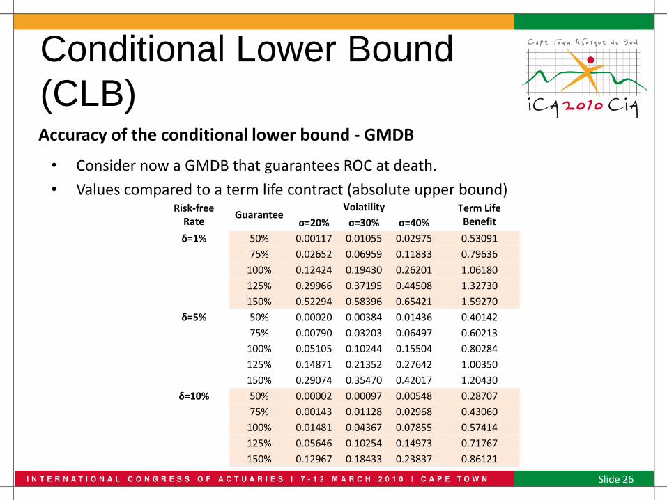
Accuracy of the conditional lower bound - GMDB
• Consider now a GMDB that guarantees ROC at death.
• Values compared to a term life contract (absolute upper bound)Risk-free
Rate Guarantee
Volatility Term Life Benefit σ=20% σ=30% σ=40%
δ=1% 50% 0.00117 0.01055 0.02975 0.53091
75% 0.02652 0.06959 0.11833 0.79636
100% 0.12424 0.19430 0.26201 1.06180
125% 0.29966 0.37195 0.44508 1.32730
150% 0.52294 0.58396 0.65421 1.59270
δ=5% 50% 0.00020 0.00384 0.01436 0.40142
75% 0.00790 0.03203 0.06497 0.60213
100% 0.05105 0.10244 0.15504 0.80284
125% 0.14871 0.21352 0.27642 1.00350
150% 0.29074 0.35470 0.42017 1.20430
δ=10% 50% 0.00002 0.00097 0.00548 0.28707
75% 0.00143 0.01128 0.02968 0.43060
100% 0.01481 0.04367 0.07855 0.57414
125% 0.05646 0.10254 0.14973 0.71767
150% 0.12967 0.18433 0.23837 0.86121

Asset-Based Charges
Slide 27
Fair value approach
• The asset-based charge for the guarantee can be solved for by equating the present value of the benefits to the present value of the contributions.
• For the pure financial contract, we therefore have:
where
1
0
0
max ,n
s lk n
k n n
k
ln
n
e e E V b
e E V P
11
0
0
1 ln
ln
ns k
k k nV
k
k
n
n n
n
V
P e r n k F b
e b F b
e

Asset-Based Charges
Slide 28
Fair value approach – GMMB & GMDB
• Similarly, we can solve the asset-based charges for the GMMB:
• For the GMDB, we have:
1
0
max ,n
s lk n
k x k n x n n
k
p e p e E V b
1 1
1
1 1
0 0
max ,n n
s k lk
k x k k x x k k k
k k
p e p q e E V b

Asset-Based Charges
Slide 29
Numerical Example
• Consider again the pure financial contract that guarantees ROC at death - annual premium of 100 over 10 years.
• Values computed for differing values of the risk-free rate and volatility.
Guarantee σ=20% σ=30% σ=40%
δ=1% 500 0.3664 2.8282 7.5429
750 6.9304 18.7686 32.8233
1000 51.1506 86.564 120.8808
δ=5% 500 0.06095 0.9881 3.4656
750 1.6931 7.187 15.1582
1000 10.5377 25.1368 41.4655
1250 48.1448 81.8928 114.5406
δ=10% 500 0.00425 0.2254 1.2115
750 0.2218 2.0356 5.7732
1000 1.7803 7.3267 15.2321
1250 6.9371 18.4198 31.8342
1500 20.2496 40.713 61.8769

Hedging
Slide 30
Mitigating risk through hedging
Some possible solutions
• Reinsurance (limited)• Structured solutions• Super-hedging• Risk-minimising strategies
Static or Dynamic? Only 1 out of 16 responded utilised a pure static hedging approach according to a Milliman survey (2008).
Other respondents used dynamic strategies or a combination.
Greeks The three main Greeks on which respondents to the Milliman survey focused were delta, rho and vega.
Further outline The CLB is used to calculate Greeks for the GMMB and GMDB products.
Greeks of CLB approximation facilitate reasonableness checks to more complex scenario based models.

Hedging
Slide 31
Calculating the Greeks
• The delta can be analytically determined.
• The delta of the embedded put option for the pure financial contract is given by:
where t is the time of valuation such that 0 ≤ t ≤ n.
1
1
0
ln
tt
st
kt nV
k
P
F t
r n t F bF k

Hedging
Slide 32
Calculating the Greeks – GMMB & GMDB
• The delta of the embedded put option for the GMMB is given by:
• The delta of the embedded put option for the GMDB is given by:
1 11
1
j x t x t
j nj
t
j
jt
t
t
Pp
Fq P
t
tt txtP
PF t
p

Hedging
Slide 33
Calculating the Greeks
• The other Greeks can be easily determined by the centre differencing approach, i.e. the rho is given by:
and the vega is given by:
• Higher order Greeks such as gamma, and other sensitivity measures can be determined in a similar way.
2
t ttt
P PP
Vega
2
t ttt
P PP

Hedging
Slide 34
Illustrative Example
Pure Financial Contract
Guarantees ROC at maturity
A payment of 1 is made monthly, i.e. ROC = 60.
Monthly Rebalancing Each month, the delta is held in the underlying fund and the remainder in the risk-free bond.
Parameters Assume a risk-free rate of 5% and volatility of 20%.
MC paths Single Monte Carlo simulation paths were used to assess the delta hedging strategy.
Hedging
Slide 35
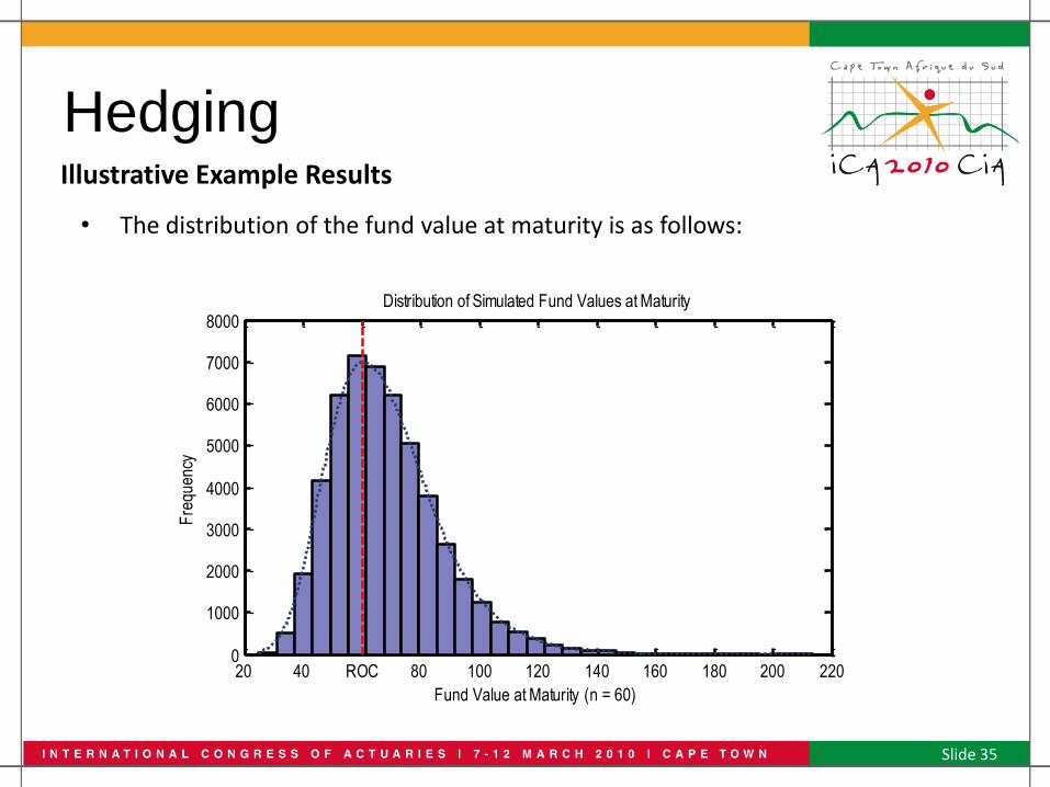
Illustrative Example Results
• The distribution of the fund value at maturity is as follows:
20 40 ROC 80 100 120 140 160 180 200 2200
1000
2000
3000
4000
5000
6000
7000
8000
Fund Value at Maturity (n = 60)
Fre
quen
cy
Distribution of Simulated Fund Values at Maturity

Hedging
Slide 36
Illustrative Example Results
• In the event of poor market performance, a likely delta hedging strategy might resemble the following:
0 10 20 30 40 50 600
10
20
30
40
50
60
Duration
Fun
d V
alue
/ H
edge
Val
ue
Hedge Performance
Fund Value
Hedge Value
Sum at Risk
Guarantee

Hedging
Slide 37
Illustrative Example Results
• In the event of good market performance, a likely delta hedging strategy might resemble the following:
0 10 20 30 40 50 600
20
40
ROC
80
100
Duration
Fun
d V
alue
/ H
edge
Val
ue
Hedge Performance
Fund Value
Hedge Value
Sum at Risk
Guarantee

Conclusions
Slide 38
Integrated risk management
Risk management should be a first consideration in product development, i.e.
IF YOU CAN’T MANAGE IT, DON’T SELL IT.
CLB a complement The CLB could act as a pragmatic complement to existing, more resource intensive, risk management processes in:
• Pricing• Reserving, and • Hedging

Contact Details
• Kobus Bekker
ABSA Life
South Africa
• Jan Dhaene
Katholieke Universiteit Leuven
Belgium
Slide 39

Good luck Bafana Bafana!
Slide 40