Hydrol. Earth Syst. Sci. Discuss., 10, 10035–10060, 2013www.hydrol-earth-syst-sci-discuss.net/10/10035/2013/doi:10.5194/hessd-10-10035-2013© Author(s) 2013. CC Attribution 3.0 License.

EGU Journal Logos (RGB)

Advances in Geosciences

Open A

ccess

Natural Hazards and Earth System

Sciences

Open A

ccess

Annales Geophysicae

Open A

ccess

Nonlinear Processes in Geophysics

Open A

ccess

Atmospheric Chemistry

and Physics

Open A

ccess

Atmospheric Chemistry

and Physics

Open A

ccess

Discussions

Atmospheric Measurement

Techniques

Open A

ccess

Atmospheric Measurement

Techniques

Open A

ccess

Discussions

Biogeosciences

Open A

ccess

Open A

ccess

BiogeosciencesDiscussions

Climate of the Past

Open A

ccess

Open A

ccess

Climate of the Past

Discussions

Earth System Dynamics

Open A

ccess

Open A

ccess

Earth System Dynamics

Discussions

GeoscientificInstrumentation

Methods andData Systems

Open A

ccess

GeoscientificInstrumentation

Methods andData Systems

Open A

ccess

Discussions

GeoscientificModel Development

Open A

ccess

Open A

ccess

GeoscientificModel Development

Discussions

Hydrology and Earth System

Sciences

Open A

ccess

Hydrology and Earth System

Sciences

Open A

ccess

Discussions

Ocean Science

Open A

ccess

Open A

ccess

Ocean ScienceDiscussions

Solid Earth

Open A

ccess

Open A

ccess

Solid EarthDiscussions

The Cryosphere

Open A

ccess

Open A

ccess

The CryosphereDiscussions

Natural Hazards and Earth System

Sciences

Open A

ccess

Discussions

This discussion paper is/has been under review for the journal Hydrology and Earth SystemSciences (HESS). Please refer to the corresponding final paper in HESS if available.

Discharge measurement with salt dilutionmethod in irrigation canals: directsampling and geophysical controls

C. Comina1, M. Lasagna1, D. A. De Luca1, and L. Sambuelli2

1Dept. of Earth Science (DST), Università degli Studi di Torino, via Valperga Caluso, 35,10125, Italy2Dept. of Environment, Land and Infrastructure Engineering (DIATI), Politecnico di Torino,corso Duca degli Abruzzi, 24, 10129, Italy

Received: 22 June 2013 – Accepted: 15 July 2013 – Published: 1 August 2013

Correspondence to: C. Comina (cesare.comina@unito.it)

Published by Copernicus Publications on behalf of the European Geosciences Union.

10035

Abstract

An important starting point for designing management improvements, particularly inirrigation areas, is to record the baseline state of the water resources, including theamount of discharge from canals. In this respect discharge measurements by meansof the salt dilution method is a traditional and well-documented technique. However,5

this methodology can be strongly influenced by the natural streaming characteristicsof the canal (e.g. laminar vs. turbulent flow) and accurate precautions must be con-sidered in the choice of both the measuring section and the length of the measuringreach of the canal which can affect the plume shape. The knowledge of plume distri-bution in the measuring cross-section is of primary importance for a correct location of10

sampling points aimed in obtaining a reliable measurement. To obtain this, geophysicalimaging of an NaCl plume from a slug-injection salt dilution test has been performedwithin this paper by means of cross-flow fast electric resistivity tomography (FERT) ina real case history. Direct sampling of the same plume has been also performed witha multisampling optimization technique to obtain an average value over the measuring15

section by means of contemporarily sampling water in nine points. Results show thata correct visualization of the passage of the salt plume is possible by means of geo-physical controls and that this can potentially help in the correct location of samplingpoints.

1 Introduction20

Improved management of water resources is becoming more and more important asseveral areas of the world suffer from water shortages. An important starting point fordesigning management improvements is to record the baseline state of the resources,including the amount of discharge from watercourses. Discharge is therefore an im-portant property and is frequently monitored along many of the major rivers, streams25

and canals. Discharge measurement by means of injection of a NaCl-solution and

10036

integration of the electrical conductivity (EC) as a function of time is a traditional andwell-documented method (salt dilution method). Alternatives for a precise dischargemeasurement may be the use of a current meter or the float method (Kalbus et al.,2006). The salt dilution technique is, however, the mostly used method in open chan-nels in investigating superficial flows, especially in remote mountainous or difficult to5

access areas where it can be hard to establish an high quality hydrologic profile, andeven harder to measure actual flow speed (Radulović et al., 2008).

Within the salt dilution method, constant-rate injection of salt is best suited for smallstreams at low flows (discharges less than about 0.1 m3 s−1), conversely slug injec-tion can be used to gauge flows up to 10 m3 s−1 or greater, depending upon channel10

characteristics (Moore, 2005).A limit of the salt dilution method is the amount of tracer to be added to increase the

conductivity at the peak of the tracer flow-through curve. This is mainly linked to thebackground level of the conductivity: if this is less than 100 µScm−1 a smaller amountof salt per m3 of runoff can be added; otherwise if the background conductivity is more15

than 500 µScm−1, more than 5 kg of salt per m3 should be used (Gees, 1990). However,given this limitation, an advantage of the method is that the measuring equipment isvery easy to move. The salt can be dissolved on site in a vessel (bucket, barrel) and itcan be directly poured from it. In this respect slug injection is more commonly used, asit requires no additional equipment. A disadvantage of this method is that only a runoff20

less than 4 m3 s−1 can be made easily, because the amount of salt to be dissolved isdifficult to handle (about 20 kg of salt for 4 m3 s−1 runoff) (Gees, 1990).

Under suitable conditions, streamflow measurements made by slug injection canbe precise within about ±5 % (Day, 1976). However, tracer-dilution method requiresa complete vertical and lateral mixing at the sampling site that needs to be assessed,25

particularly in linear irrigation canals, like in the present case study. Vertical mixingis usually accomplished very rapidly compared to lateral mixing (Rantz, 1982). Fre-quently, long reaches are needed for complete lateral mixing of the tracer. The mixingdistance will vary however also with the hydraulic characteristics of the reach (e.g.

10037

laminar vs. turbulent flow). When the slug injection method is used, complete mixing isconsidered to have occurred when the area under the concentration-time curve has thesame value at all points in the downstream sampling section (Rantz, 1982). Generally,an optimum mixing length is the one that produces mixing adequate for an accuratedischarge measurement but does not require an excessively long duration of sampling.5

If adequate mixing is known to exist at a given sampling site, the tracer cloud in the sluginjection method must be sampled for its entire time of passage (from the time of itsfirst appearance until the time of its disappearance) at several locations throughout thesampling cross section of the channel (Rantz, 1982). Experience indicates that regard-less of method or stream size, at least three lateral sampling points should be used at10

each sampling site (Rantz, 1982).Alternatively, to obtain a direct visualization of the tracer plume and then a proper

location of the monitoring points, indirect geophysical measurements could be used,aimed at imaging the passage of the NaCl solution in the monitored section. In thisrespect process tomography, in the forms of electrical resistivity tomography (ERT) has15

been developed in the last decades of the 20th century as a tool for monitoring bi-phase or multi-phase mixtures flows in numerous applications (Xie et al., 1995; Tappand Wilson, 1997). Tomographic methods, and their interpretation based on the elec-trical properties of water mixtures, are appealing in numerous applications since theycan be used, for example, to image component concentration distributions and de-20

tect transient dynamic changes in multi-phase processes. Moreover they can also givequantitative evaluations about the properties of imaged mixtures. In this respect vari-ous relationships can be found in the literature relating the electrical resistivity to thephysico-chemical properties of the mixture.

Most of the applications of this technique (Fangary et al., 1998; Lucas et al., 1999;25

Wang and Cilliers 1999; Yang and Liu 2000; Warsito and Fan, 2001) deal with cylin-drical flows bodies (in pipes, cyclones, tanks) and the electrodes are placed on oneor more circumferences orthogonal to the cylinder axis. This geometrical configura-tion assures an optimum conditioning of the inverse tomographic problem but however

10038

limits its applicability to real case studies on natural rivers or channels. Some previousstudies have been already carried out assessing the possibility of recognising the pres-ence of granular materials in slow water flows (Sambuelli et al., 2002) and in imagingsolid and pollutants transport characteristics in fast water flows (Sambuelli and Comina,2010) in situations where the imaged body cannot be entirely surrounded by electrodes5

as in the case of creeks, rivers and canals.The objective of this study is therefore to evidence the real distribution of a NaCl

plume from a slug-injection salt dilution test in a test cross section, by means of cross-flow fast electric resistivity tomography (FERT), and to evaluate the effect that a nonuniform tracer cloud could have on an incorrect location of the monitoring points in10

the cross section. In this respect the application of the same technique presented inSambuelli and Comina (2010) is reported in a real case history in order to monitor thesalt plume used for discharge measurement with the salt dilution method in slug injec-tion approach. A sampling optimization in the downstream sampling section was alsotested, sampling the canal water in different points of the cross section, and obtaining15

an average value over the sampled area by means of a contemporary water picking up.

2 Material and methods

After a brief introduction on the test site, the conceptual basis and field proceduresfor slug injection using salt dilution method and geophysical controls are hereafter ex-posed. Particularly the water multi-sampling system, proposed for the optimization of20

the tracer quantitative detection, is described together with the field procedures neces-sary for the execution of electric tomographies.

2.1 The study area: the Osasco Canal

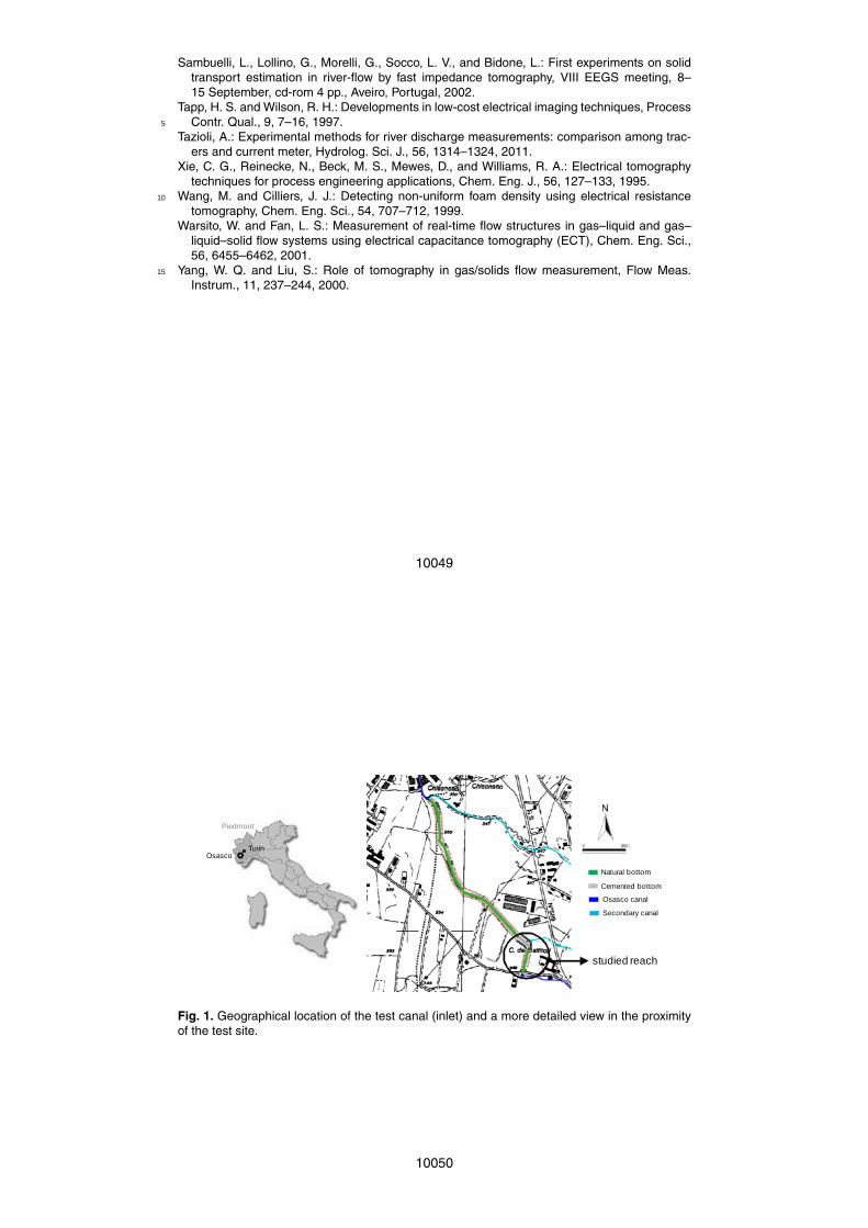
The Osasco Canal is an irrigation canal located in Piedmont (north-western Italy). Ithas an overall length of about 7 km and carries water from the Chisone River (Fig. 1).25

10039

The investigated canal reach, in which direct measurements and geophysical controlswere made, has a length of about 100 m, an average width of 2 m and about 0.5 waterlevel. The Osasco Canal has a gross average discharge of 0.5 m3 s−1, estimated witha current meter, and a water EC of about 170 µScm−1 (Clemente et al., 2013; Perottiet al., 2013).5

Some pictures of both the sampling and the injection points are reported in Fig. 2.In this portion the bottom of the channel is cobbled (gravels and cobbles) and cementless except for a small portion immediately upstream of the chosen injection point,where a small cemented weir is located (Fig. 2). The measuring section is locatedunder a small road bridge and a canal curve is placed immediately downstream of this10

section (Fig. 2). A part from injection and measuring sections the canal is difficult toaccess due to dense vegetation growing on the banks.

2.2 Canal reach choice

Following precautions for the salt dilution method, the most appropriate canal reachhas been selected for the execution of the tests (Figs. 1 and 2) considering that:15

a. the reach should not have dead water between the injection and sampling points:the storage and slow release of tracer from those areas greatly prolongs the timerequired to the entire salt cloud to pass at the sampling site;

b. the sampling site has to be free of excessive turbulence; indeed EC measure-ments are adversely affected by the presence of air bubbles (Fig. 2);20

c. an injection point that is turbulent enough to ensure virtually instantaneous mixingis to be chosen; this condition is not always easy to be achieved especially inirrigation canals where laminar flow can be predominating (Fig. 2);

d. the background EC level of the river is to be stable during the measuring time;

e. it is important to identify an optimum mixing length for a given canal reach; too25

short distances will result in an inaccurate accounting of the tracer mass passing10040

the sampling site, conversely, too great a distances will yield excellent results, butonly if it is feasible to sample for a long enough period (Rantz, 1982).

2.3 Slug injection method with sampling optimization

The slug injection method required the instantaneous injection of a slug of tracer solu-tion and the accounting of the total mass of tracer at the sampling cross section. Com-5

mon salt (NaCl) was used as tracer; it is the most frequently used chemical tracer andprovides the best results (Drost, 1989; Kumar and Nachiappan, 2000; Tazioli, 2011). Itindeed meets all the criteria for a tracer: is (a) “chemically conservative”, i.e., does notadsorb (“chemically bind”) onto river sediments, (b) has a high solubility in water, (c) isrelatively non-toxic, (d) can be measured in the field indirectly with a conductivity me-10

ter, and (e) is relatively cheap and readily available. In this study a NaCl mass of 9 kgwas dissolved in a barrel within about 30 L of water and this slug was instantaneouslyinjected into the canal at the injection point (Fig. 2).

The slug of tracer solution instantaneously injected into the canal produceda concentration-time curve in the downstream sampling cross section. Given this ex-15

perimental curve the equation for computing stream discharge, which is based on theprinciple of the conservation of mass, is (Rantz,1982):

Q =V0 ·C0∫∞

0 (C−Cb)dt

where Q is the discharge of the canal, V0 is the volume of the tracer solution injectedinto the canal, C0 is the concentration of this solution, C is the measured tracer con-20

centration at a given time at the downstream sampling site and Cb is the backgroundconcentration of the canal.

The term∫∞

0 (C−Cb)dt globally represents the total area under the concentration-time curve. To experimentally obtain this curve, the passage of the entire tracer cloudwas monitored by continuously measuring the EC value of the channel water at the25

10041

sampling section, to determine the relationship between EC and time. The elapsedtime between subsequent measures of EC was 5 s. The basic principles is that theion concentration of the slug injected increases the natural water concentration, (C−Cb) can be viewed as an “incremental” concentration with respect to the background,consequently increases also the measured electrical conductivity which can be used5

as an index of the salt concentration. Indeed, over a wide range of concentrations theEC is directly proportional to salt concentration (Radulović et al., 2008; Moore, 2005;Gees, 1990; Rantz, 1982). The recorded values of EC were then transformed intoconcentration values through the use of a laboratory estimated calibration line. Thiscalibration was constructed measuring the variation of EC in the water canal to the10

addition of different amounts of NaCl. In this way the “incremental concentration” inrespect to the natural water conductivity, which is used as reference, is obtained. Theexample calibration line for the present study is reported in Fig. 3.

Tracer-dilution measurements require a complete tracer mixing at the sampling site.However, the detection of the tracer is often performed in only one point, normally15

central to the sampling cross section. This procedure can create some mistakes in thecalculation of canals discharge if the injection solution is not fully mixed across thechannel at the downstream sampling section.

In order to make the EC values more representative of the entire sampling crosssection and to obtain the optimization of quantitative detection, a water multi-sampling20

system was devised. This system was realized by means of a framework of steel rods towhich 9 tubes of small diameter are connected. The tubes are linked to a water pumpwhich spills the water of the canal simultaneously from the 9 measuring points. Theobjective of this apparatus is to allow for a more uniformly distributed sampling pointsthrough the whole section of the canal; however due to the accessibility of the mea-25

sured section (different water depths along it) and to the manoeuvrability of the wholesystem, only a portion of the section has been sampled. A scheme of the adoptedmulti-sampling system and of its location is reported in Fig. 4.

10042

2.4 Cross-flow FERT

Cross-flow FERT has been used as an independent tool for monitoring the executionof salt dilution tests and have been executed by means of an array of 16 underwaterelectrodes (14 on the canal bottom and 2 on his sides). The electric cable has beenanchored on the canal bottom by means of appropriate weights and the position of each5

electrode together with the shape of the section has been measured. An example ofthe electrodes disposition scheme for the test site and a picture of the array is reportedin Fig. 5.

The electric cable has been connected to an AC acquiring device (CIT Iridium Italys.a.s.) injecting a sinusoidal current at 916 Hz. The CIT is a very fast acquisition device10

with 16 bit resolution. Indeed the instrument can execute approximately 20 acquisitionsper second (at the selected operative frequency) so that the acquisition of a singletomographic image can be performed in a relatively fast time. A devoted acquisition se-quence consisting of a total of 227 quadrupoles (both dipole-dipole and Wenner types)has been used. In this way it is possible to appreciate variations in concentration also15

for relatively fast transient phenomena. The acquisitions have been performed continu-ously for about 5 min after the impulse plume has been injected in the canal. The timerequired for the acquisition of a single image is of the order of 30 s for the experimentalsetup of this study, including also saving the file and starting up the new measure-ment, therefore the total number of processed images, during the passage of the salt20

plume, is 9. Data have been inverted by means of an on purpose designed software(NES Electric Arbitrary 2-D Closed Geometry by Andrea Borsic) which is based ona damped least squares inversion algorithm.

A representation based on the relative difference in electric resistivity (ER) amongthe several images has been adopted in the following. Reference was made to the25

“clear water” condition by subtracting the resistivity distributions obtained at each timestep to a reference image of the canal water measured before the slug injection (ERof 58Ωm coherently corresponding to the inverse of the directly measured EC). In

10043

this way the passage of the salt plume is expected to provide an overall reduction inresistivity (increased concentration of the salt plume) over the images. Indeed ER isthe inverse of EC, so that symmetrical considerations can be made in respect to hisbehaviour with increasing salt concentration. The same laboratory calibration curveused for the salt dilution method has been later used to convert the resistivity maps in5

salt concentration maps.

3 Results and discussion

The NaCl curve of the direct sampling with the adopted multi-sampling system is re-ported in Fig. 6; given the equations reported in the previous paragraph, this curvehighlight a discharge equal to 0.46 m3 s−1. For convenience of comparison with the10

results of cross-flow FERT data have been converted in ER and an indication of theaverage time of acquisition of each tomographic image is also reported in the samefigure.

The results of some acquired images during the passage of the salt plume are in-stead presented in Fig. 7; some of the images, with very similar ER distribution, have15

been suppressed (dashed lines in Fig. 6) for easiness of visualization. In these imagesthe ER difference with respect to the “clear water” condition (image at time 25 s) arereported. Images are very clear in the recognition of the passage of the plume, iden-tified with a strong resistivity reduction. This reduction is quite homogeneous in theearly times, in correspondence to the higher salt concentration in the transient plume,20

but appears more concentrated in some zones of the canal in late times. Noticeablythe left side of the reconstructed resistivity image (which is upstream the canal curve)appears not affected by the passage of the plume. This has been also observed on siteby visual inspection of the passing plume. The imaged reduction in resistivity showsaverage values around about 25Ωm, even if localized higher values are present in the25

map. These values seems little lower with respect to the direct sampled curve which

10044

instead reports a peak of about 40Ωm reduction with respect to the canal “clear water”resistivity (Fig. 6).

The resistivity images acquired have been then interpreted in order to extract quan-titative information about the salt concentration. Such interpreted data are reported inFig. 8 for the same sampling intervals of Fig. 7 and in Fig. 9 in a 3-D representation.5

The salt plume is clearly evidenced in both images. However, with respect to the pre-vious images, some localized peaks in concentration appear more evidently related tothe laminar flow of the canal. Particularly in the 3-D visualization it appears clear thatthe “coda” of the plume are located along the banks of the canal. Indeed the velocity offlow varies from zero at the walls to a maximum along the center. This reflects in two10

main concentration peaks located on both sides of the measuring section and only oneof them appears correctly sampled by the direct method since the sampling grid hasbeen placed nearer to the left downstream bank (Fig. 4).

By extracting mean and standard deviation values of concentration in every tomo-graphic image it is also possible to estimate a time-concentration curve also from geo-15

physical measurements. This interpretation is reported in Fig. 10 and compared to theone obtained from direct measurements. The mass balance of the injected salt ex-tracted from the two evaluations (i.e. direct sampling and cross-flow FERT) partiallydiffers, the mean value of cross-flow FERT data report globally a lower concentrationpeak. There are several reasons to explain the observed differences:20

– the concentration extracted from cross-flow FERT is an integral concentration overa measuring time (30 s) which is higher than the one used for direct sampling(5 s); this will probably result in a reduced peak value given the fast phenomenonin observation;

– the reduced peak concentration observed by cross-flow FERT may be also related25

to the smoothing of the inversion algorithm adopted which does not allow for toosharp variations in concentration; it must indeed be noted the increased dimen-sions of standard deviation error-bars near the peak of the plume with respect

10045

to a more homogeneous situation towards the end of it; this implies that whenthe concentration distribution within the section is sharp the inverse solution hasincreased variability;

– cross-flow FERT conversely images the whole section of the canal (included theleft bank where there appear to be a reduced concentration area) in respect to5

the direct sampling technique and therefore seems globally more reliable;

– direct sampling can be affected by localized high concentration points which couldinfluence the overall estimate; data of cross-flow FERT seems indeed to be betterin agreement if the maximum concentration value is considered (dashed red linein Fig. 10).10

In order to assess the likelihood of this last reason, a comparison between directsampling and cross-flow FERT been performed, over the same sampling area of thecanal. In this respect Fig. 11 reports an image of the plume in correspondence of thesampling grid at the time of passage of the main concentration peak. It can be notedthat most of the spilling points appears located near to high concentration peaks and15

therefore the average concentration curve may be biased towards higher values. Pro-viding similar images preliminary to the design of the sampling grid could be thereforea strong help in establishing the most correct measurement protocol.

4 Conclusions

Direct sampling of the NaCl plume from a slug-injection salt dilution test and geophys-20

ical imaging of the same salt plume, by means of cross-flow fast electric resistivitytomography (FERT), have been compared in this work. Direct sampling has been per-formed with a multisampling optimization in the downstream section, obtaining an av-erage value over the sampled stream section, using a contemporary water sampling;geophysical data have been acquired and interpreted independently.25

10046

Results shows that the reconstructed curve from cross-flow FERT seems affectedfrom an overall lower sensitivity in respect to the peak passage of the plume and there-fore mass balance estimations based on these data cannot be completely reliable.Nevertheless cross-flow FERT has provided a good qualitative visualization of the pas-sage of the plume in the imaged section and, since the knowledge of tracer distribution5

in the cross-section is very important for a correct location of sampling points, canbe used as a preliminary control in order to establish the best position for accuratedischarge measurements by means of the direct sampling method.

Following this first visualization, a sampling optimization in the downstream samplingsection, using a multisampling technique, can be strongly recommended. This method,10

sampling the canal water in different points of the cross section, by means of a con-temporary water picking up, can indeed optimize the quantitative detection and resultin more reliable discharge estimates.

Acknowledgements. This research has been partially funded in the framework of a researchproject between the Agricultural Management of Piedmont Region and the Earth Science De-15

partment of Università degli Studi di Torino. Authors are indebted with Paolo Clemente, Gio-vanna Dino, Diego Franco, Francesco Marzano and Sabrina Bonetto for their help in the exe-cution of the field tests.

References

Clemente, P., De Luca, D. A., Dino, G. A., and Lasagna, M.: Water losses from irrigation canals20

evaluation: comparison among different methodologies, Geophys. Res. Abstr., EGU2013-9024, EGU General Assembly 2013, Vienna, Austria, 2013.

Day, T. J.: On the precision of salt dilution gauging, J. Hydrol., 31, 293–306, 1976.Drost, J. W.: Single-Well and Multi-Well Nuclear Tracer Techniques – a Critical Review, Tech-

nical Documents in Hydrology, International Hydrological Programme, 96, UNESCO, Paris,25

1989.

10047

Fangary, Y. S., Williams, R. A., Neil, W. A., Bond, J., and Faulks, I.: Application of electricresistance tomography to detect deposition in hydraulic conveying systems, Powder Technol.,95, 61–66, 1998.

Gees, A.: Flow measurement under difficult measuring conditions: Field experience with thesalt dilution method, in: Hydrology in Mountainous Regions I. Hydrological Measurements;5

The Water Cycle, edited by: Lang, H. and Musy, A., IAHS Publ., 193, 255–262, 1990.Kalbus, E., Reinstorf, F., and Schirmer, M.: Measuring methods for groundwater – surface water

interactions: a review, Hydrol. Earth Syst. Sci., 10, 873–887, doi:10.5194/hess-10-873-2006,2006.

Kumar, B. and Nachiappan, R. P.: Estimation of alluvial aquifer parameters by a single-well10

dilution technique using isotopic and chemical tracers: a comparison, in: Tracers and Mod-elling in Hydrogeology, IAHS Publ. 262, edited by: Dassargues, A., IAHS Press, Wallingford,53–56, 2000.

Lucas, G. P., Cory, J., Waterfall, R. C., Loh, W. W., and Dickin, F. J.: Measurement of the solidsvolume fraction and velocity distributions in solids–liquid flows using dual-plane electrical15

resistance tomography, Flow Meas. Instrum., 10, 249–258, 1999.Moore, R. D.: Slug injection using salt in solution, Streamline Watershed Management Bulletin,

8, 1–6, 2005.Perotti, L., Clemente, P., De Luca, D. A., Dino, G. A., and Lasagna, M.: Remote sensing and

hydrogeological methodologies for irrigation canal leakage detection: the Osasco and Fos-20

sano test sites (Northwestern Italy), Geophys. Res. Abstr., EGU2013-5705, EGU GeneralAssembly 2013, Vienna, Austria, 2013.

Radulović, M., Radojević, D., Dević, D., and Blečić, M.: Discharge calculation of the spring us-ing salt dilution method – application site Bolje Sestre Spring (Montenegro), available at: http://balwois.com/balwois/administration/full_paper/ffp-1257.pdf (last access: 24 July 2013),25

2008.Rantz, S. E.: Measurement and Computation of Streamflow: Volume 1. Measurement of Stage

and Discharge, US Geological Survey Water-Supply Paper 2175, US Department of theInterior, US Government Printing Office, Washington, DC, 1982.

Sambuelli, L. and Comina, C.: Fast ert to estimate pollutants and solid transport variation in30

water flow: a laboratory experiment, B. Geofis. Teor. Appl., 51, 1–22, 2010.

10048

Sambuelli, L., Lollino, G., Morelli, G., Socco, L. V., and Bidone, L.: First experiments on solidtransport estimation in river-flow by fast impedance tomography, VIII EEGS meeting, 8–15 September, cd-rom 4 pp., Aveiro, Portugal, 2002.

Tapp, H. S. and Wilson, R. H.: Developments in low-cost electrical imaging techniques, ProcessContr. Qual., 9, 7–16, 1997.5

Tazioli, A.: Experimental methods for river discharge measurements: comparison among trac-ers and current meter, Hydrolog. Sci. J., 56, 1314–1324, 2011.

Xie, C. G., Reinecke, N., Beck, M. S., Mewes, D., and Williams, R. A.: Electrical tomographytechniques for process engineering applications, Chem. Eng. J., 56, 127–133, 1995.

Wang, M. and Cilliers, J. J.: Detecting non-uniform foam density using electrical resistance10

tomography, Chem. Eng. Sci., 54, 707–712, 1999.Warsito, W. and Fan, L. S.: Measurement of real-time flow structures in gas–liquid and gas–

liquid–solid flow systems using electrical capacitance tomography (ECT), Chem. Eng. Sci.,56, 6455–6462, 2001.

Yang, W. Q. and Liu, S.: Role of tomography in gas/solids flow measurement, Flow Meas.15

Instrum., 11, 237–244, 2000.

10049

19

LIST OF FIGURES

studied reach

Natural bottom

Cemented bottom

Osasco canal

Secondary canal

Piedmont

OsascoTurin

Figure 1. Geographical location of the test canal (inlet) and a more detailed view

in the proximity of the test site. Fig. 1. Geographical location of the test canal (inlet) and a more detailed view in the proximityof the test site.

10050

20

Natural bottom

Cemented bottom

Osasco canal

Secondary canal

slug injection

measuring section

b)

a)

Figure 2. Tested canal reach: a) injection point at the end of a cemented weir and

b) measuring section, under a small road bridge and before a canal curve.

Fig. 2. Tested canal reach: (a) injection point at the end of a cemented weir and (b) measuringsection, under a small road bridge and before a canal curve.

10051

21

0

0.05

0.1

0.15

0.2

0.25

0.3

0.35

0.4

0.45

100 200 300 400 500 600 700 800 900 1000

Increm

ental con

centration

(g/l)

Conductivity (microS/cm) Figure 3. Calibration curve for converting EC measured data to concentration

values with reference to the natural water electrical conductivity (170 µS/cm). Fig. 3. Calibration curve for converting EC measured data to concentration values with refer-ence to the natural water electrical conductivity (170 µScm−1).

10052

22

x [m]

y [m

]

pump and sampling apparatus

sampling grid

0.3 m

0.6 m

Figure 4. Multi-sampling system with details of the sampling grid (black circles

are water spilling points) and of the pumping apparatus; the below section is seen from up-stream.

Fig. 4. Multi-sampling system with details of the sampling grid (black circles are water spillingpoints) and of the pumping apparatus; the below section is seen from up-stream.

10053

23

x [m]

y [m

]

electrodes

ballast weigths

Figure 5. Electrodes disposition for cross-flow FERT: images of the electrodes

and the anchoring system (top) and of the mesh used for the inversion (bottom), the below section is seen from up-stream.

1

Res

istiv

ity[O

m.m

]

Time [s]

2 3 4 5 6 7 8 9 10

102030405060

0 50 100 150 200 250 300 350

Figure 6. Time-resistivity curve determined with the multisampling apparatus

and indication of the time of execution of the cross-flow FERT images presented in Figure 7 (full lines).

Fig. 5. Electrodes disposition for cross-flow FERT: images of the electrodes and the anchoringsystem (top) and of the mesh used for the inversion (bottom), the below section is seen fromup-stream.

10054

23

x [m]

y [m

]

electrodes

ballast weigths

Figure 5. Electrodes disposition for cross-flow FERT: images of the electrodes

and the anchoring system (top) and of the mesh used for the inversion (bottom), the below section is seen from up-stream.

1R

esis

tivity

[Om

.m]

Time [s]

2 3 4 5 6 7 8 9 10

102030405060

0 50 100 150 200 250 300 350

Figure 6. Time-resistivity curve determined with the multisampling apparatus

and indication of the time of execution of the cross-flow FERT images presented in Figure 7 (full lines).

Fig. 6. Time-resistivity curve determined with the multisampling apparatus and indication of thenumber and time of execution of the cross-flow FERT images presented in Figs. 7 and 8 (fulllines).

10055

24

0 0.5 1 1.5 2 2.5-0.4-0.3-0.2-0.1

0

0 0.5 1 1.5 2 2.5-0.4-0.3-0.2-0.1

0

0 0.5 1 1.5 2 2.5-0.4-0.3-0.2-0.1

0

-25-24-23-22-21-20-19-18-17-16-15-14-13-12-11-10-9-8-7-6-5-4-3-2-10

0 0.5 1 1.5 2 2.5-0.4-0.3-0.2-0.1

0

0 0.5 1 1.5 2 2.5-0.4-0.3-0.2-0.1

0

resi

stiv

ity d

iffer

ence

[ohm

.m]

0 0.5 1 1.5 2 2.5-0.4-0.3-0.2-0.1

0

1

3

5

6

8

10

x [m]

y [m

]y

[m]

y [m

]y

[m]

y [m

]y

[m]

Figure 7. Electric resistivity differences in the imaged section for increasing

times with reference to Figure 6, seen from up-stream. Fig. 7. Electric resistivity differences in the imaged section for increasing times, image numberwith reference to Fig. 6, seen from up-stream.

10056

25

0 0.5 1 1.5 2 2.5-0.4-0.3-0.2-0.1

0

0 0.5 1 1.5 2 2.5-0.4-0.3-0.2-0.1

0

0 0.5 1 1.5 2 2.5-0.4-0.3-0.2-0.1

0

0 0.5 1 1.5 2 2.5-0.4-0.3-0.2-0.1

0

0 0.5 1 1.5 2 2.5-0.4-0.3-0.2-0.1

0

0 0.5 1 1.5 2 2.5-0.4-0.3-0.2-0.1

0

1

3

5

6

8

10

x [m]

y [m

]y

[m]

y [m

]y

[m]

y [m

]y

[m] 0

0.01

0.02

0.03

0.04

0.05

0.06

0.07

0.08

0.09

0.1

0.11

0.12

0.13

0.14

0.15

Incr

emen

tal N

aCl c

once

ntra

tion

[gr/l

]

Figure 8. Incremental concentrations in the imaged section for increasing times

with reference to Figure 6, seen from up-stream.

Fig. 8. Incremental concentrations in the imaged section for increasing times, image numberwith reference to Fig. 6, seen from up-stream.

10057

26

Figure 9. 3D visualization of the passage of the salt plume in the studied canal

section.

0

0.05

0.1

0.15

0.2

0.25

0.3

0 50 100 150 200 250 300 350

Incr

emen

tal N

aCl c

once

ntra

tion

[ gr /

l ]

time [s]

Direct samplingCross-flow ERT meanCross-flow ERT max

Figure 10. Comparison of direct sampling and cross-flow FERT obtained

concentration curves; the dashed red line refers to the maximum concentration value determined from cross-flow FERT in the area of the canal reported in Figure 11.

Fig. 9. 3-D visualization of the passage of the salt plume in the studied canal section.

10058

26

Figure 9. 3D visualization of the passage of the salt plume in the studied canal

section.

0

0.05

0.1

0.15

0.2

0.25

0.3

0 50 100 150 200 250 300 350

Incr

emen

tal N

aCl c

once

ntra

tion

[ gr /

l ]

time [s]

Direct samplingCross-flow ERT meanCross-flow ERT max

Figure 10. Comparison of direct sampling and cross-flow FERT obtained

concentration curves; the dashed red line refers to the maximum concentration value determined from cross-flow FERT in the area of the canal reported in Figure 11.

Fig. 10. Comparison of direct sampling and cross-flow FERT obtained concentration curves;the dashed red line refers to the maximum concentration value determined from cross-flowFERT in the area of the canal reported in Fig. 11.

10059

27

Incr

emen

tal N

aCl c

once

ntra

tion

[gr/l

]

0.5 0.6 0.7 0.8 0.9 1 1.1 1.2 1.3 1.4 1.5-0.4

-0.3

-0.2

-0.1

0

0

0.01

0.02

0.03

0.04

0.05

0.06

0.07

0.08

0.09

0.1

x [m]

y [m

]

Figure 11. Comparison of direct sampling (black circles are water spilling

points) and cross-flow FERT over the same sampling area at the time of passage of the main plume.

Fig. 11. Comparison of direct sampling (black circles are water spilling points) and cross-flowFERT over the same sampling area at the time of passage of the main plume.

10060