1001.2678

arX

iv:1

001.

2678

v3 [

q-fi

n.PR

] 1

8 Se

p 20

12

Arbitrage bounds for prices of weighted variance swaps ∗

Mark Davis† Jan Ob loj‡ Vimal Raval§

Abstract

We develop a theory of robust pricing and hedging of a weighted variance swap given marketprices for a finite number of co–maturing put options. We assume the put option prices do notadmit arbitrage and deduce no-arbitrage bounds on the weighted variance swap along with super-and sub- replicating strategies that enforce them. We find that market quotes for variance swaps aresurprisingly close to the model-free lower bounds we determine. We solve the problem by transformingit into an analogous question for a European option with a convex payoff. The lower bound becomesa problem in semi-infinite linear programming which we solve in detail. The upper bound is explicit.

We work in a model-independent and probability-free setup. In particular we use and extendFollmer’s pathwise stochastic calculus. Appropriate notions of arbitrage and admissibility are intro-duced. This allows us to establish the usual hedging relation between the variance swap and the ‘logcontract’ and similar connections for weighted variance swaps. Our results take form of a FTAP: weshow that the absence of (weak) arbitrage is equivalent to the existence of a classical model whichreproduces the observed prices via risk–neutral expectations of discounted payoffs.

Key Words: Weighted variance swap, weak arbitrage, arbitrage conditions, model-independentbounds, pathwise Ito calculus, semi-infinite linear programming, fundamental theorem of asset pric-ing, model error.

1 Introduction

In the practice of quantitative finance, the risks of ‘model error’ are by now universally appreciated.Different models, each perfectly calibrated to market prices of a set of liquidly traded instruments, maygive widely different prices for contracts outside the calibration set. The implied hedging strategies,even for contracts within the calibration set, can vary from accurate to useless, depending on how wellthe model captures the sample path behaviour of the hedging instruments. This fundamental prob-lem has motivated a large body of research ranging from asset pricing through portfolio optimisation,risk management to macroeconomics (see for example Cont (2006), Follmer et al. (2009), Acciaio et al.(2011), Hansen and Sargent (2010) and the references therein). Another stream of literature, to whichthis paper is a contribution, develops a robust approach to mathematical finance, see Hobson (1998),Davis and Hobson (2007), Cox and Ob loj (2011a). In contrast to the classical approach, no probabilisticsetup is assumed. Instead we suppose we are given current market quotes for the underlying assets andsome liquidly traded options. We are interested in no-arbitrage bounds on a price of an option impliedby this market information. Further, we want to understand if, and how, such bounds may be enforced,in a model-independent way, through hedging.

In the present paper we consider robust pricing and hedging of a weighted variance swap when pricesof a finite number of co–maturing put options are given. If (St, t ∈ [0, T ]) denotes the price of a financialasset, the weighted realized variance is defined as

(1.1) RVT =

n∑

i=1

h(Sti)

(

logSti

Sti−1

)2

,

where ti is a pre-specified sequence of times 0 = t0 < t1 < · · · < tn = T , in practice often daily sampling,and h is a given weight function. A weighted variance swap is a forward contract in which cash amounts

∗This paper was previously circulated under the title “Arbitrage Bounds for Prices of Options on Realized Variance.”†Department of Mathematics, Imperial College London, London SW72AZ, UK ([email protected]).‡Mathematical Institute, Oxford-Man Institute of Quantitative Finance and St John’s College, University of Oxford,

Oxford OX1 3LB, UK ([email protected])§Imperial College London. Work supported by EPSRC under a Doctoral Training Award.

1

http://arxiv.org/abs/1001.2678v3

Arbitrage bounds for prices of options on realised variance 2

equal to A × RVT and A × PRV

T are exchanged at time T , where A is the dollar value of one variancepoint and PRV

T is the variance swap ‘price’, agreed at time 0. Three representative cases considered inthis paper are the plain vanilla variance swap h(s) ≡ 1, the corridor variance swap h(s) = 1I(s) where Iis a possibly semi-infinite interval in R+, and the gamma swap in which h(s) = s. The reader can consultGatheral (2006) for information about variance swaps and more extended discussion of the basic factspresented below. In this section we restrict the discussion to the vanilla variance swap; we return to theother contracts in Section 4.

In the classical approach, if we model St under a risk-neutral measure Q as1 St = Ft exp(Xt−12 〈X〉t),

where Ft is the forward price (assumed to be continuous and of bounded variation) and Xt is a continuousmartingale with quadratic variation process 〈X〉t, then St is a continuous semimartingale and

logSti

Sti−1

= (g(ti) − g(ti−1)) + (Xti −Xti−1),

with g(t) = log(Fti)−12 〈X〉ti . For m = 1, 2 . . . let smi , i = 0, . . . , km be the ordered set of stopping times

in [0, T ] containing the times ti together with times τm0 = 0, τmk = inft > τmk−1 : |Xt −Xτmk−1

| > 2−m

wherever these are smaller than T . If RV mT denotes the realized variance computed as in (1.1) but using

the times smi , then RVmT → 〈X〉T = 〈log S〉T almost surely, see Rogers and Williams (2000), Theorem

IV.30.1. For this reason, most of the pricing literature on realized variance studies the continuous-timelimit 〈X〉T rather than the finite sum (1.1) and we continue the tradition in this paper.

The key insight into the analysis of variance derivatives in the continuous limit was provided byNeuberger (1994). We outline the arguments here, see Section 4 for all the details. With St as above andf a C2 function, it follows from the general Ito formula that Yt = f(St) is a continuous semimartingalewith d〈Y 〉t = (f ′(St))

2d〈S〉t. In particular, with the above notation

d(log St) =1

StdSt −

1

2S2t

d〈S〉t =1

StdSt −

1

2d〈log S〉t,

so that

(1.2) 〈logS〉T = 2

∫ T

0

1

StdSt − 2 log(ST /S0)

This shows that the realized variation is replicated by a portfolio consisting of a self-financing tradingstrategy that invests a constant $2DT in the underlying asset S together with a European option whoseexercise value at time T is λ(ST ) = −2 log(ST /FT ). Here DT is the time-T discount factor. Assumingthat the stochastic integral is a martingale, (1.2) shows that the risk-neutral value of the variance swaprate PRV

T is

(1.3) PRV

T = E

[

〈log S〉T]

= −2E[log(ST /FT )] = 21

DTPlog,

that is, the variance swap rate is equal to the forward value Plog/DT of two ‘log contracts’—Europeanoptions with exercise value − log(ST /FT ), a convex function of ST . (1.3) gives us a way to evaluate PRV

T

in any given model. The next step is to rephrase Plog in terms of call and put prices only.Recall that for a convex function f : R+ → R the recipe f ′′(a, b] = f ′

+(b) − f ′+(a) defines a positive

measure f ′′(dx) on B(R+), equal to f ′′(x)dx if f is C2. We then have the Taylor formula

(1.4) f(x) = f(x0) + f ′+(x0)(x− x0) +

∫ x0

0

(y − x)+ν(dy) +

∫ ∞

x0

(x − y)+f ′′(dy).

Applying this formula with x = ST , x0 = FT and f(s) = log(s/S0), and combining with (1.2) gives

(1.5)1

2〈log S〉T =

∫ T

0

1

StdSt − log(FT /S0) + 1 − ST /FT +

∫ FT

0

(K − ST )+

K2dK +

∫ ∞

FT

(ST −K)+

K2dK.

Assuming that puts and calls are available for all strikes K ∈ R+ at traded prices PK , CK , (1.5) providesa perfect hedge for the realized variance in terms of self-financing dynamic trading in the underlying (the

1For example, St = (e(r−q)tS0)(eσWt−

12σ2t) in the Black-Scholes model, with the conventional notation.


first four terms) and a static portfolio of puts and calls and hence uniquely specifies the variance swaprate PRV

T as

(1.6) PRV

T =2

DT

∫ ∞

0

1

K2(PK1(K≤FT ) + CK1(K>FT ))dK.

Our objective in this paper is to investigate the situation where, as in reality, puts and calls areavailable at only a finite number of strikes. In this case we cannot expect to get a unique value for PRV

T

as in (1.6). However, from (1.2) we expect to obtain arbitrage bounds on PRV

T from bounds on the valueof the log contract—a European option whose exercise value is the convex function − log(ST /FT ). Itwill turn out that the weighted variance swaps we consider are associated in a similar way with otherconvex functions. In Davis and Hobson (2007) conditions were stated under which a given set of prices(P1, . . . , Pn) for put options with strikes (K1, . . . ,Kn) all maturing at the same time T is consistentwith absence of arbitrage. Thus the first essential question we have to answer is: given a set of putprices consistent with absence of arbitrage and a convex function λT , what is the range of prices Pλ fora European option with exercise value λT (ST ) such that this option does not introduce arbitrage whentraded in addition to the existing puts? We answer this question in Section 3 following a statement ofthe standing assumptions and a summary of the Davis and Hobson (2007) results in Section 2.

The basic technique in Section 3 is to apply the duality theory of semi-infinite linear programmingto obtain the values of the most expensive sub-replicating portfolio and the cheapest super-replicatingportfolio, where the portfolios in question contain static positions in the put options and dynamic tradingin the underlying asset. The results for the lower and upper bounds are given in Propositions 3.1 and3.5 respectively. (Often, in particular in the case of plain vanilla variance swaps, the upper boundis infinite.) For completeness, we state and prove the fundamental Karlin-Isii duality theorem in anappendix, Appendix A. With these results in hand, the arbitrage conditions are stated and proved inTheorem 3.6.

In this first part of the paper—Sections 2 and 3—we are concerned exclusively with European optionswhose exercise value depends only on the asset price ST at the common exercise time T . In this casethe sample path properties of St, t ∈ [0, T ] play no role and the only relevant feature of a ‘model’is the marginal distribution of ST . For this reason we make no assumptions about the sample paths.When we come to the second part of the paper, Sections 4 and 5, analysing weighted variance swaps,then of course the sample path properties are of fundamental importance. Our minimal assumption isthat St, t ∈ [0, T ] is continuous in t. However, this is not enough to make sense out of the problem.The connection between the variance swap and the ‘log contract’, given at (1.2), is based on stochasticcalculus, assuming that St is a continuous semimartingale. In our case the starting point is simply a setof prices. No model is provided, but we have to define what we mean by the continuous-time limit of therealized variance and by continuous time trading. An appropriate framework is the pathwise stochasticcalculus of Follmer (1981) where the quadratic variation and an Ito-like integral are defined for a certainsubset Q of the space of continuous functions C[0, T ]. Then (1.2) holds for S(·) ∈ Q and we have theconnection we sought between variance swap and log contract. For weighted variance swaps the sameconnection exists, replacing ‘− log’ by some other convex function λT , as long as the latter is C2. In thecase of the corridor variance swap, however, λ′′T is discontinuous and we need to restrict ourselves to asmaller class of paths L for which the Ito formula is valid for functions in the Sobolev space W2. All of thisis consistent with models in which St is a continuous semimartingale, since then Pω : S(·, ω) ∈ L = 1.We discuss these matters in a separate appendix, Appendix B.

With these preliminaries in hand we formulate and prove, in Section 4 the main result of the paper,Theorem 4.3, giving conditions under which the quoted price of a weighted variance swap is consistentwith the prices of existing calls and puts in the market, assuming the latter are arbitrage-free. When theconditions fail there is a weak arbitrage, and we identify strategies that realize it.

In mathematical finance it is generally the case that option bounds based on super- and sub-replicationare of limited value because the gap is too wide. However, here we know that as the number of put optionsincreases then in the limit there is only one price, namely, for a vanilla variance swap, the number PRV

T

of (1.6), so we may expect that in a market containing a reasonable number of liquidly-traded puts thebounds will be tight. In Section 5 we present data from the S&P500 index options market which showsthat our computed lower bounds are surprisingly close to the quoted variance swap prices.

This paper leaves many related questions unanswered. In particular we would like to know whathappens when there is more than one exercise time T , and how the results are affected if we allow jumpsin the price path. The latter question is considered in the small time-to-expiry limit in the recent paperKeller-Ressel and Muhle-Karbe (2011). A paper more in the spirit of ours, but taking a complementary


approach, is Hobson and Klimmek (2011)[HK] . In our paper the variance swap payoff is defined by thecontinuous-time limit, and we assume that prices of a finite number of traded put and/or call prices areknown. By contrast, HK deal with the real variance swap contract (i.e., discrete sampling) but assumethat put and call prices are known for all strikes K ∈ R+, so in practice the results will depend on howthe traded prices are interpolated and extrapolated to create the whole volatility surface. Importantly,HK allow for jumps in the price process; this is indeed the main focus of their work. The price boundsthey obtain are sharp in the continuous-sampling limit. Combining our methods with those of HK wouldbe an interesting, and possibly quite challenging, direction for future research, see Remark 4.6 below.

Exact pricing formulas for a wide variety of contracts on discretely-sampled realized variance, in ageneral Levy process setting, are provided in Crosby and Davis (2011).

2 Problem formulation

Let (St, t ∈ [0, T ]) be the price of a traded financial asset, which is assumed non-negative: St ∈ R+ =[0,∞). In addition to this underlying asset, various derivative securities as detailed below are also traded.All of these derivatives are European contracts maturing at the same time T . The present time is 0. Wemake the following standing assumptions as in Davis and Hobson (2007):(i) The market is frictionless: assets can be traded in arbitrary amounts, short or long, without transactioncosts, and the interest rates for borrowing and lending are the same.(ii) There is no interest rate volatility. We denote by Dt the market discount factor for time t, i.e. theprice at time 0 of a zero-coupon bond maturing at t.(iii) There is a uniquely-defined forward price Ft for delivery of one unit of the asset at time t. This willbe the case if the asset pays no dividends or if, for example, it has a deterministic dividend yield. We letΓt denote the number of shares that will be owned at time t if dividend income is re-invested in shares;then F0 = S0 and Ft = S0/(DtΓt) for t > 0.

We suppose that n put options with strikes 0 < K1 < . . . < Kn and maturity T are traded, attime-0 prices P1, . . . , Pn. In (Davis and Hobson, 2007), the arbitrage relations among these prices wereinvestigated. The facts are as follows. A static portfolio X is simply a linear combination of the tradedassets, with weights π1, . . . , πn, φ, ψ on the options, on the underlying asset and on cash respectively, itbeing assumed that dividend income is re-invested in shares. The value of the portfolio at maturity is

(2.1) XT =

n∑

i=1

πi[Ki − ST ]+ + φΓTST + ψD−1T

and the set-up cost at time 0 is

(2.2) X0 =n∑

i=1

πiPi + φS0 + ψ.

Note that it does not make any sense a priori to speak about Xt – the value of the portfolio at anyintermediate time – as this is not determined by the market input and we do not assume the optionsare quoted in the market at intermediate dates t ∈ (0, T ). To make sense to statements like “XT isnon-negative” we need to specify the universe of scenarios we consider. Later, in Section 4, this will meanthe space of of possible paths (St : t ≤ T ). However here, since we only allow static trading as in (2.1),we essentially look at a one–period model and we just need to specify the possibly range of values for ST

and we suppose that ST may take any value in [0,∞).A model M is a filtered probability space (Ω,F = (Ft)t∈[0,T ],P) together with a positive F-adapted

process (St)t∈[0,T ] such that S0 coincides with the given time-0 asset price. Given market prices of options,we say that M is a market model for these options if Mt = St/Ft is an F-martingale (in particular, St isintegrable) and the market prices equal to the P–expectations of discounted payoffs. In particular, M is amarket model for put options if Pi = DTE[Ki−ST ]+ for i = 1, . . . , n. We simply say that M is a marketmodel if the set of market options with given prices is clear from the context. It follows that in a marketmodel we have joint dynamics on [0, T ] of all assets’ prices such that the initial prices agree with themarket quotes and the discounted prices are martingales. By the (easy part of the) First FundamentalTheorem of Asset Pricing (Delbaen and Schachermayer, 1994) the dynamics do not admit arbitrage.

Our main interest in the existence of a market model and we want to characterise it in terms of thegiven market quoted prices. This requires notions of arbitrage in absence of a model. We say that thereis model-independent arbitrage if one can form a portfolio with a negative setup cost and a non-negative


α

r2

r1

k1 k2 1 k3

r3

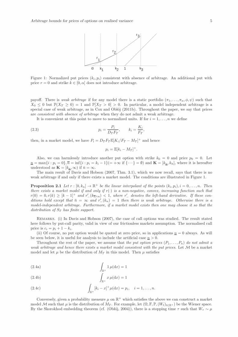
Figure 1: Normalized put prices (ki, pi) consistent with absence of arbitrage. An additional put withprice r = 0 and strike k ∈ [0, α] does not introduce arbitrage.

payoff. There is weak arbitrage if for any model there is a static portfolio (π1, . . . , πn, φ, ψ) such thatX0 ≤ 0 but P(XT ≥ 0) = 1 and P[XT > 0] > 0. In particular, a model independent arbitrage is aspecial case of weak arbitrage, as in Cox and Ob loj (2011b). Throughout the paper, we say that pricesare consistent with absence of arbitrage when they do not admit a weak arbitrage.

It is convenient at this point to move to normalized units. If for i = 1, . . . , n we define

(2.3) pi =Pi

DTFT, ki =

Ki

FT,

then, in a market model, we have Pi = DTFTE[Ki/FT −MT ]+ and hence

pi = E[ki −MT ]+.

Also, we can harmlessly introduce another put option with strike k0 = 0 and price p0 = 0. Letn = maxi : pi = 0,n = infi : pi = ki − 1(= +∞ if · · · = ∅) and K = [kn, kn], where it is hereafterunderstood as K = [kn,∞) if n = ∞.

The main result of Davis and Hobson (2007, Thm. 3.1), which we now recall, says that there is noweak arbitrage if and only if there exists a market model. The conditions are illustrated in Figure 1.

Proposition 2.1 Let r : [0, kn] → R+ be the linear interpolant of the points (ki, pi), i = 0, . . . , n. Thenthere exists a market model if and only if r(·) is a non-negative, convex, increasing function such thatr(0) = 0, r(k) ≥ [k − 1]+ and r′−(kn∧n) < 1, where r′− denotes the left-hand derivative. If these con-ditions hold except that n = ∞ and r′−(kn) = 1 then there is weak arbitrage. Otherwise there is amodel-independent arbitrage. Furthermore, if a market model exists then one may choose it so that thedistribution of ST has finite support.

Remarks. (i) In Davis and Hobson (2007), the case of call options was studied. The result statedhere follows by put-call parity, valid in view of our frictionless markets assumption. The normalised callprice is ci = pi + 1 − ki.

(ii) Of course, no put option would be quoted at zero price, so in applications n = 0 always. As willbe seen below, it is useful for analysis to include the artificial case n > 0.

Throughout the rest of the paper, we assume that the put option prices (P1, . . . , Pn) do not admit aweak arbitrage and hence there exists a market model consistent with the put prices. Let M be a marketmodel and let µ be the distribution of MT in this model. Then µ satisfies

∫

R+

1µ(dx) = 1(2.4a)

∫

R+

xµ(dx) = 1(2.4b)

∫

R+

[ki − x]+µ(dx) = pi, i = 1, . . . , n.(2.4c)

Conversely, given a probability measure µ on R+ which satisfies the above we can construct a marketmodel M such that µ is the distribution of MT . For example, let (Ω,F,P, (Wt)t∈R+) be the Wiener space.By the Skorokhod embedding theorem (cf. (Ob loj, 2004)), there is a stopping time τ such that Wτ ∼ µ


and (Wτ∧t) is a uniformly integrable martingale. It follows that we can put Mt = 1 + Wτ∧(t/(T−t)) fort ∈ [0, T ). This argument shows that the search for a market model reduces to a search for a measure µsatisfying (2.4). We will denote by MP the set of measures µ satisfying the conditions (2.4).

Lemma 2.2 For any µ ∈ MP , µ(R+\K) = 0.

Proof. That µ[0, kn) = 0 when n > 0 follows from (2.4c) with i = n. When n ≤ n we have cn = 0, i.e.there is a free call option with strike kn and we conclude that µ(kn,∞) = 0.

The question we wish to address is whether, when prices of additional options are quoted, consistencywith absence of arbitrage is maintained. As discussed in Section 1, we start by considering the case whereone extra option is included, a European option maturing at T with convex payoff.

3 Hedging convex payoffs

Suppose that, in addition to the n put options, a European option is offered at price Pλ at time 0, withexercise value λT (ST ) at time T , where λT is a convex function. We can obtain lower and upper boundson the price of λT by constructing sub-replicating and super-replicating static portfolios in the othertraded assets. These bounds are given in Sections 3.1 and 3.2 respectively and are combined in Section3.3 to obtain the arbitrage conditions on the price Pλ.

We work in normalised units throughout, that is, the static portfolios have time-T values that arelinear combinations of cash, underlying MT and option exercise values [ki −MT ]+. The prices of unitsof these components at time 0 are DT , DT and DT pi respectively, where a unit of cash is $1. Indeed, toprice MT observe that $1 invested in the underlying at time 0 yields ΓTST /S0 = ST /FTDT = MT/DT

at time T . To achieve a consistent normalization for λT we define the convex function λ as

(3.1) λ(x) =1

FTλT (FTx).

In a market model M we have Pλ = DTE[λT (ST )] = DTFTE[λ(MT )], so the normalized price is

pλ =Pλ

DTFT= E[λ(MT )]

and the cost for delivering a payoff λ(MT ) is DT pλ.

3.1 Lower bound

A sub-replicating portfolio is a static portfolio formed at time 0 such that its value at time T is majorizedby λ(MT ) for all values of MT . Obviously, a necessary condition for absence of model independentarbitrage is that DT pλ be not less than the set-up cost of any sub-replicating portfolio. It turns outthat the options ki with i ≤ n or i ≥ n are redundant, so the assets in the portfolio are indexed byk = 1, . . . ,m where

m = (n+ 1) ∧ n− n+ 1

and the time-T values of these assets, as functions of x = MT are

a1(x) = 1 (Cash)

a2(x) = x (Underlying)(3.2)

ai+2(x) = [kn+i − x]+, i = 1, . . . ,m− 2 (Options).

We let a(x) be the m-vector with components ak(x). Note that am(x) is equal to [kn−1 − x]+ if n ≤ nand to [kn −x]+ otherwise. The set-up costs for the components in (3.2), as observed above, are DT , DT

and DT pn+i respectively. The corresponding forward prices are as in (2.4):

b1 = 1

b2 = 1(3.3)

bi+2 = pn+i, i = 1, . . . ,m− 2.

We let b denote the m-vector of the forward prices. A static portfolio is defined by a vector y whose kthcomponent is the number of units of the kth asset in the portfolio. The forward set-up cost is yTb andthe value at T is yTa(MT ).


With this notation, the problem of determining the most expensive sub-replicating portfolio is equiv-alent to solving the (primal) semi-infinite linear program

PLB : supy∈Rm

yTb subject to yTa(x) ≤ λ(x) ∀x ∈ K.

The constraints are enforced only for x ∈ K. If n > 0 [n ≤ n] we have a free put with strike kn [call withstrike kn] and, since λ is convex, we can extend the sub-replicating portfolio to all of R+ at no cost.

The key result here is the basic duality theorem of semi-infinite linear programming, due to Isii (1960)and Karlin, see Karlin and Studden (1966). This theorem, stated as Theorem A.1, and its proof are givenin Appendix A. The dual program corresponding to PLB is

DLB : infµ∈M

∫

K

λ(x)µ(dx) subject to

∫

K

a(x)µ(dx) = b0,

where M is the set of Borel measures such that each ai is integrable. The constraints in DLB can beexpressed as µ satisfying (2.4) for n < i < n. This is simply equivalent to µ ∈ MP since, as shown inLemma 2.2, any µ ∈ MP has support in K. Let V L

P and V LD be the values of the primal and dual problems

respectively. It is a general and easily proved fact that V LP ≤ V L

D . The ‘duality gap’ is V LD − V L

P . TheKarlin-Isii theorem gives conditions under which there is no duality gap and we have existence in PLB.

Proposition 3.1 We suppose as above that λ(x) is a convex function on R+, finite for all x > 0, andthat (ki, pi) is a set of normalised put option strike and price pairs which do not admit a weak arbitrage.If λ(x) is unbounded as x→ 0 and n = 0 then we further assume that p1/k1 < p2/k2. Then V

LD = V L

P andthere exists a maximising vector y. The most expensive sub-replicating portfolio of a European option withpayoff λT (ST ) at maturity T is the static portfolio X† as in (2.1) with weights ψ† = FTDT y1, φ

† = y2/ΓT ,

π†n+i = y2+i for i = 1, . . . ,m− 2 and π†

i = 0 otherwise. For this portfolio, X†0 = DTFTV

LD .

If there is existence in the dual problem DLB then there is an optimal measure µ† which is a finitelinear combination of Dirac measures µ† =

∑mj=1 wjδxj

(dx) such that each interval [kj , kj+1) contains atmost one point xj. For this measure

(3.4) µ†(x) > 0 ⇒ X†T

∣

∣

∣

ST=FT x=

n∑

i=1

π†i [Ki − FTx]+ + φ†ΓTFTx+ ψ†D−1

T = λT (FTx).

Proof. The first part of the proposition is an application of Theorem A.1. The primal problem PLB

is feasible because any support line corresponds to a portfolio (containing no options). The functionsa1, . . . , am are linearly independent. Recall from Proposition 2.1 that if (ki, pi) do not admit weakarbitrage then there is a measure µ satisfying the conditions (2.4) and such that µ is a finite weighted sumof Dirac measures. It follows that

∫

R+ |λ(x)|µ(dx) <∞ unless one of the Dirac measures is placed at x = 0and λ is unbounded at zero. If n > 0 then there is no mass on the interval [0, n), hence none at zero. Whenn = 0 we always have p1/k1 ≤ p2/k2. If p1/k1 = p2/k2 then the payoff [k2−MT ]+−k2[k1−MT ]+/k1 hasnull cost and is strictly positive on (0, k2). Since p1 > 0 there must be some mass to the left of k1, and thismass must be placed at 0, else there is an arbitrage opportunity. But then

∫

λdµ = +∞ and V LD = +∞.

The condition in the proposition excludes this case. In every other case there is a realizing measure µ suchthat µ(0) = 0. Indeed, if p1/k1 < p2/k2 then the extended set of put prices (k, 0), (k1, p1), . . . , (kn, pn)is consistent with absence of arbitrage if k ∈ [0, α], where α = (k1p2−k2p1)/(p2−p1) (see Figure 1). Anymodel realizing these prices puts weight 0 on the interval [0, k). Thus V L

D is finite under the conditions wehave stated. It remains to verify that the vector b belongs to the interior of the moment cone Mm definedat (A.1). For this, it suffices to note that for all i such that ki ∈ (kn, kn) it holds that [ki− 1]+ < pi < ki,and so the condition is satisfied. We now conclude from Theorem A.1 that V L

P = V LD and that we have

existence in the primal problem. The expressions for ψ† etc. follow from the relationships (2.3) betweennormalized and un-normalized prices.

Assume now that the dual problem has a solution. Any optimal measure µ† ∈ MP satisfies

∫

K

λ(x)µ†(dx) = infµ∈MP

∫

K

λ(x)µ(dx)

.

Recall K = [kn, kn] and partition K into intervals In+1, . . . , In∧n+1 defined by

Ii = [ki−1, ki) for i = n+ 1, . . . n ∧ n and In∧n+1 = [kn∧n, kn),


so In∧n+1 = ∅ if n ≤ n. Lemma 3.2 below asserts that we may take µ† atomic with at most one atom ineach of the intervals Ii. By definition the optimal subhedging portfolio X† satisfies X†

T ≤ λT (ST ) while

our duality result shows that the µ† expectations of these random variables coincide. Hence X†T = λT (ST )

a.s. for MT = ST /FT distributed according to µ†, and (3.4) follows.

Lemma 3.2 Let µ ∈ MP and suppose∫

K|λ(x)|µ(dx) <∞. Define

(3.5) Iµ = i ≤ n ∧ n+ 1|µ(Ii) > 0.

Now let µ′ be the measure

µ′ =∑

i∈Iµ

µ(Ii)δxi,

in which δx denotes the Dirac measure at x, and for an index i ∈ I, xi =

∫Ii

xdµ(x)

µ(Ii). Then µ′ ∈ MP and

(3.6)

∫

K

λ(x)µ′(dx) ≤

∫

K

λ(x)µ(dx).

Proof of lemma: The inequality (3.6) follows from the conditional Jensen inequality. A direct com-putation shows that µ′ satisfies (2.4), so that µ′ ∈ MP .

It remains now to understand when there is existence in the dual problem. We exclude the case whenλT is affine on some [z,∞) which is tedious. We characterise the existence of a dual minimiser in termsof properties of the solution to the primal problem and also present a set of sufficient conditions. Of theconditions given, (i) would never be encountered in practice (it implies the existence of free call options)and (iii),(iv) depend only on the function λT and not on the put prices Pi. The examples presented inSection 3.1.1 show that if these conditions fail there may still be existence, but this will now depend onthe Pi. Condition (ii) is closer to being necessary and sufficient, but is not stated in terms of the basicdata of the problem.

Proposition 3.3 Assume λT is not affine on some half-line [z,∞). Then, in the setup of Proposition3.1, the existence of a minimiser in the dual problem DLB fails if and only if

(3.7) n = ∞ and X†T

∣

∣

∣

ST=s= φ†ΓT s+ ψ†D−1

T < λT (s), for all s ≥ Kn.

In particular, each of the following is a sufficient condition for existence of a minimiser in DLB:

(i) n <∞;

(ii) we have

(3.8) X†T

∣

∣

∣

ST=Kn

= φ†ΓTKn + ψ†D−1T < λT (Kn) and lim

s→∞λT (s) − φ†ΓT s = ∞;

(iii) for any y < λT (Kn) there is some x > Kn such that the point (Kn, y) lies on a support line to λTat x;

(iv) λT satisfies

(3.9)

∫ ∞

0

xλ′′T (dx) = +∞ .

Proof: We consider two cases.

Case 1: n ≤ n, i.e. condition (i) holds. In this case the support of any measure µ ∈ MP is containedin the finite union In+1 ∪ · · · ∪ In of bounded intervals, and

∑ni=n+1 µ(Ii) = 1. Further, pn−1 > kn − 1

and (2.4b) together imply that µ(In) > 0. Let µj , j = 1, 2, . . . be a sequence of measures such that

∫

K

λ(x)µj(dx) → infµ∈MP

∫

K

λ(x)µ(dx)

as j → ∞.

By Lemma 3.2, we may and do assume that each µj is atomic with at most one atom per interval. Wedenote wi

j = µj(Ii) and let xij denote the location of the atom in Ii. For definiteness, let xij = ∆, where


∆ is some isolated point, if µj has no atom in Ii, i.e., if wij = 0. Let A be the set of indices i such that xij

converges to ∆ as j → ∞, i.e. xij 6= ∆ for only finitely many j, and let B be the complementary set of

indices. Then there exists j∗ such that∑

i∈B wij = 1 for j > j∗. Because the wi

j and xij are contained in

compact intervals there exists a subsequence jk, k = 1, 2 . . . and points wi∗, x

i∗ such that wi

jk→ wi

∗ and

xijk → xi∗ as k → ∞. It is clear that∑

i∈B wi∗ = 1 and that

V LD = lim

k→∞

∫

K

λ(x)µjk (dx) =

∫

K

λ(x)µ†(dx)

where µ†(dx) =∑

i∈B wi∗δxi

∗(dx). Similarly, the integrals of 1, x and [ki − x]+ converge, so µ† ∈ MP .

Finally, since the intervals Ii are open on the right, it is possible that xi∗ ∈ Ii+1. If also xi+1∗ ∈ Ii+1 we

can invoke Lemma 3.2 to conclude that this 2-point distribution in Ii+1 can be replaced by a 1-pointdistribution without increasing the integral. Thus µ† retains the property of being an atomic measurewith at most one atom per interval. We have existence in the dual problem and, by the arguments above,X†

T = λT (ST ) dµ†-a.s.

Case 2: n = ∞. Let X†T (s) denote the payoff of the portfolio X† at time T when ST = s. Suppose that

a minimiser µ† exists in DLB, which we may take as atomic. Since n = ∞ there exists x ∈ (kn,∞) such

that µ†(x) > 0 and hence, by (3.4), X†T (FTx) = λ(FT x). This shows that (3.7) fails since FTx > Kn.

It remains to show the converse: that if n = ∞ but (3.7) fails then a minimiser µ† exists. Given

our assumption on λT , if (3.7) fails then K† := sups ≥ 0 : X†T (s) = λT (s) ∈ [Kn,∞). We continue

with analysis similar to Case 1 above. Here we have intervals In, . . . , In covering Kn = [kn, kn), but alsoa further interval In+1 = [kn,∞) which does not necessarily have zero mass. Since In+1 is unbounded,the argument above needs some modification. We take a minimizing sequence of point mass measuresµj as in Case 1. If xn+1

j converge (on a subsequence) to a finite xn+1∗ then we can restrict our attention

to a compact [0, xn+1∗ + 1] and everything works as in Case 1 above. Suppose to the contrary that

lim inf xn+1j = ∞, as j → ∞. We first apply the arguments in Case 1 to the sequence µj of restrictions

of µj to Kn. Everything is the same as above except that now∑

i wij ≤ 1. A subsequence converges to a

sub-probability measure µ† on Kn, equal to a weighted sum of Dirac measures as above. Define µ† = µ†

if ι1 ≡ µ†(Kn) = 1 and otherwise µ† = µ† + (1 − ι1)δx, where x ∈ In+1 is to be determined. Whateverthe value of x, µ† satisfies conditions (2.4a) and (2.4c) (the put values depend only on µ†).

Since µj ∈ MP ,∑n+1

i=1 wijx

ij = 1 and in particular

1 −n∑

i=1

wijx

ij ≥ wn+1

j kn.

Taking the limit along the subsequence we conclude that

(3.10) 1 −n∑

i=1

wi∗x

i∗ ≥ kn

(

1 −n∑

i=1

wi∗

)

= kn(1 − ι1).

By the convergence argument of Case 1, ι2 ≡∫ kn

0xµ†(dx) ≤ 1. If ι1 < 1 we have only to choose

x = (1 − ι2)/(1 − ι1) to ensure that the ‘forward’ condition (2.4b) is also satisfied. The inequality (3.10)guarantees that x ≥ kn. Thus µ† ∈ MP and, since n = ∞, x > kn and hence K† > Kn.

We now show that the complementary case ι1 = 1 contradicts K† ∈ [Kn,∞). Indeed, if ι1 = 1 wehave, since n = ∞,

kn − 1 < pn =

∫ ∞

0

[kn − x]+µ†(dx) =

∫ kn

0

(kn − x)µ†(dx) = kn −n∑

i=1

wi∗x

i∗ .

Observe that then

(3.11) wn+1j xn+1

j = 1 −n∑

i=1

wijx

ij −−−→

j→∞1 −

n∑

i=1

wi∗x

i∗ = pn − kn + 1 > 0.

Since K† ∈ [Kn,∞), taking γ = λ′T (K† + 1) −X†T

′(K† + 1) = λ′T (K† + 1) − φ†ΓT > 0, we have

(3.12) λT (s) −X†T (s) ≥ γ(s−K† + 1), ∀s ≥ K† + 1.


Define now a new function λT by

λT (s) = λT (s)1s≤K† + (φ†ΓT s+ ψ†D−1T )1s>K†

so that we haveX† ≤ λT (ST ) ≤ λT (ST ) and, by definition, for ST > K† we haveX† = λT (ST ) < λT (ST ).It follows that X† is also the most expensive subreplicating portfolio for λT (s) and hence the primal anddual problems for λ and for λ(x) = 1

FTλT (FTx) have all the same value. Writing this explicitly and using

(3.12) and(3.11) gives:

0 = limj→∞

∫ ∞

0

(λ(x) − λ(x))µj(dx) = limj→∞

(λ(xn+1j ) − λ(xn+1

j ))wn+1j

≥ limj→∞

γ(xn+1j −K† − 1)wn+1

j = γ(pn − kn + 1) > 0,

a contradiction.We turn to showing that each of (i)–(iv) is sufficient for existence of a dual minimiser µ†. 2 Obviously

n <∞ is sufficient as observed above. We now show that either of (ii) or (iii) implies that K† ∈ [Kn,∞)

and that (3.12) holds. In the light of the arguments above this will be sufficient. X†T (s) is linear on

[Kn,∞) and λT is convex hence the difference of the two either converges to a constant or divergesto infinity. In the latter case the difference grows quicker than a linear function, more precisely (3.12)holds. The former case is explicitly excluded in (ii) and is contradictory with (iii) as the line ℓ(s) :=

φ†ΓT s + ψ†D−1T + limu→∞(λT (u) −X†

T (u)) is asymptotically tangential to λT (s) as s → ∞ and hencethe condition in (iii) is violated for any y < ℓ(Kn). In particular, it follows that K† < Kn then we canadd to X† a positive number of call options with strike Kn and obtain a subreplicating portfolio withan initial cost strictly larger (recall that n = ∞) than X† which contradicts the optimality of X†. Thiscompletes the proof that either (ii) or (iii) is sufficient for existence.

Finally, we argue that (iii) and (iv) are equivalent. In (iii) the point x satisfies

λT (x) + ξ(Kn − x) = y, for some ξ ∈ [λ′T (x−), λ′T (x+)].

This equation has a solution x for all y < λT (Kn) if and only if limx→∞ λT (x) − xλ′T (x) = −∞. Theequivalence with (iv) follows integrating by parts

∫ ∞

Kn

xλ′′T (dx) =(

xλ′T (x) − λT (x))∣

∣

∣

∞

Kn

.

3.1.1 Examples with one put option

We consider now examples in which just one put option price is specified. We illustrate different caseswhen existence in the dual problem holds or fails. For simplicity assume all prices are normalised, i.e.DT = FT = 1, and we are given only a single put option with strike k = 1.2. The convex function takesthe form λ(x) = 1/x+ axb. Computation of the most expensive sub-hedging portfolio can be done by asimple search procedure.

Consider first the case a = 0, so that λ(x) = 1/x. The results are shown in Figure 2 with data shownin Table 1: p is the put price, x0, x1 the points of tangency, w0, w1 the implied probability weights onx0, x1 and ψ, φ the units of, respectively, cash and forward in the portfolio.

p = 0.4 is a ‘regular’ case: we have tangent lines at x0, x1 and the solution to the dual problem putsweights 8/9, 1/9 respectively on these points. As p increases it is advantageous to include more puts inthe portfolio, so x1 increases. At p = 0.6 we reach a boundary case where ψ = φ = 0, and the put iscorrectly priced by the Dirac measure with weight 1 at x0 = 0.6 = k/2. Obviously, this measure doesnot correctly price the forward, but it does correctly price the portfolio since φ = 0. When p > 0.6, theonly way to increase the put component further is to take ψ < 0 (and then clearly the optimal value ofφ is 0.) When p = 0.7 the optimal value is ψ = −0.8 and we find that in this and every other such casethe implied weight is w0 = 1, as the general theory predicts.

Next, take a = 0.25, b = 1, so that λ(x) = 1/x+0.25x, has its minimum at x = 2 and is asymptoticallylinear. We take p = 0.7. Taking the expectation with respect to the limiting measure µ† gives the valueof the lower sub-hedge in Figure 3, but this is not optimal: we can add a maximum number 0.25 of call


p x0 x1 value ψ φ w0 w1

0.4 0.75 3 1.2222 0.6667 -0.1111 0.8889 0.11110.6 0.6 - 1.6667 0 0 1.00 -0.7 0.5 - 2.00 -0.8 0 1.00 -

Table 1: Data for Figure 2

0 0.5 1 1.5 2 2.5 3 3.5 4 4.5 5−1

0

1

2

3

4

5

p=0.6p=0.7

p=0.4

Figure 2: Most expensive subhedging portfolios for λ(x) = 1/x given a single put option with strike 1.2and prices p = 0.4, 0.6, 0.7

options, which have positive value, giving the upper sub-hedge in Figure 3. This is optimal, but does notcorrespond to any dual measure.

Finally, let a = 0.0625, b = 2, giving λ(x) = 1/x + 0.0625x2. The minimum is still at x = 2 but λis asymptotically quadratic. This function satisfies condition (iii) of Proposition 3.3 and there is dualexistence for every arbitrage-free value of p. The optimal portfolio for p = 0.7 is shown in Figure 4.

3.2 Upper bound

To compute the cheapest super-replicating portfolio we have to solve the linear program

PUB : infy∈Rm

yTb subject to yTa(x) ≥ λ(x) ∀x ∈ K.

The corresponding dual program is

DUB : supµ∈M

∫

K

λ(x)µ(dx) subject to

∫

K

a(x)µ(dx) = b,

where, by Lemma 2.2, we may replace K by R+. By (1.4) we have for x ∈ R+

λ(x) = λ(1) + λ′(1+)(x− 1) +

∫

(0,1]

[k − x]+λ′′(dk) +

∫

(1,∞)

[x− k]+λ′′(dk).

Consider µ ∈ MP and let pµ(k) =∫

[k − x]+µ(dx), cµ(k) =∫

[x− k]+µ(dk) be the (normalised) prices ofputs and calls. Integrating the above against µ gives

(3.13)

∫

λ(x)µ(dx) = λ(1) +

∫

(0,1]

pµ(k)λ′′(dk) +

∫

(1,∞)

cµ(k)λ′′(dk).

Recall that cµ(k) = pµ(k)+1−k and hence maximising in cµ(k) or in pµ(k) is the same. pµ(k) is a convexfunction dominated by the linear interpolation of points (ki, pi), i = 0, 1, . . . , n, extended to the right of(kn, pn) with slope 1. Since we assume the given put prices do not admit weak arbitrage, it follows from

2In fact for this part of the Proposition we do not need to impose any additional conditions on λT apart from convexity.


0 2 4 6 8 10−1

0

1

2

3

4

5

6

Figure 3: The most expensive subhedging portfolio (upper dashed line) for λ(x) = 1/x + 0.25x givena single put option with strike 1.2 and price p = 0.7. The lower dashed line is the portfolio priced at∫

λ(x)µ†(dx) which is suboptimal.

0 2 4 6 8 10−2

−1

0

1

2

3

4

5

6

7

Figure 4: Most expensive subhedging portfolios for λ(x) = 1/x+ 0.0625x2 given a single put option withstrike 1.2 and price p = 0.7.

(Davis and Hobson, 2007) (see also Proposition 2.1 above) that this upper bound is attained either exactlyor in the limit. More precisely, if n = ∞ one can take µz ∈ MP supported on kn, , . . . , , kn, z, for z largeenough, which attain the upper bound on [0, kn] and asymptotically induce the upper bound on (kn,∞)as z → ∞. It follows from (3.13) that the value of the dual problem is V U

D = limz→∞

∫

Kλ(x)µz(dx).

If n ≤ n one can take z = kn and µknattains the upper bound. It follows from (3.13) that then

V UD =

∫

Kλ(x)µkn

(dx).From this observations, one expects that y – the solution to the primal problem – will correspond to

a (normalised) portfolio yTa(x) which linearly interpolates (ki, λ(ki)), i = kn, . . . , n ∧ n and (if n = ∞)extends linearly to the right as to dominate λ(k). The function x 7→ yTa(x) is piecewise linear with afinite number of pieces and no such function can majorize the convex function λ over R+ unless λ(0) <∞and λ′(∞) = γ <∞. In general we impose:

(a) n > 0 or(

n = 0 and λ(0) <∞)

and

(b) n ≤ n or(

n = ∞ and λ′(∞) <∞)

.(3.14)

We have the following result.

Proposition 3.4 If condition (3.14) holds then there exists a solution y to the linear program PUB . Thefunction yTa(x) is the linear interpolation of the points (kn, λ(kn)), , . . . , (kn∧n, λ(kn∧n)) together with,


if n = ∞, the line l(x) = yTa(kn) + (x− kn)λ′(∞) for x ≥ kn. Primal and dual problem have the samevalue V P

U = V DU and the existence of a maximiser in the dual problem fails if and only if n = ∞ and λ

is not affine on [kn,∞).If the condition (3.14) is not satisfied, there is no feasible solution and V D

U = ∞.

Proof. As argued above, (3.14) is a necessary condition for existence of a feasible solution. Suppose,for example, that n = ∞ = λ′(∞). Then (z − kn)µz(z) = cn and hence zµz(z) → cn as z → ∞.Together with λ′(∞) = ∞ this implies that V D

U = ∞. Other cases are similar.Suppose (3.14) holds and first consider the case when n = ∞. λ is bounded on [kn, kn] and the linear

interpolation is well defined as is the extension beyond kn. Further, there exists some constant δ suchthat yTa(x) − λ(x) ≤ δ for all x ∈ R+. The weight y2+j on the jth put option is the change in slopeat kn+j , the ‘underlying’ weight y2 is equal to γ, and at x = kn we have λn = y1 + y2kn, so the ‘cash’weight is y1 = λn − knγ. The value of the objective function is, by definition,

yTb =

∫

R+

yTa(x)µ(dx),

for any µ ∈ MP . In particular, since yTa(ki) = λ(ki), taking z large enough, we have

yTb0 =

∫

R+

yTa(x)µz(dx) =

n∑

i=n

λ(ki)µz(ki) + yTa(z)µz(z)

=

∫

R+

λ(x)µz(dx) + (yTa(z) − λ(z))µz(z) ≤

∫

R+

λ(x)µz(dx) + δµ(z).

(3.15)

Recall that∫

xµz(dx) = 1 and in particular µ(z) → 0 as z → ∞. Taking the limit as z → ∞ in theabove, we conclude that yTb0 ≤ V U

D . The basic inequality V UD ≤ V U

P between the primal and dual valuesthen implies that y is optimal for PUB and V U

D = V UP . The existence of the solution to DUB fails unless

there exists z ≥ kn with yTa(z) = λ(z), which happens if and only if λ(z) is affine on [kn,∞).When n ≤ n the arguments are analogous, except that now we need to ensure yTa(x) ≥ λ(x) only for

x ∈ K = [kn, kn]. The dual problem has a maximiser as observed in the remarks above the Proposition.The primal problem also has a solution y but it is not unique. Indeed, let y0 = (−kn, 1, 0, . . . , 0, 1) andobserve that y0T

b = 0 and y0T

a(x) ≡ 0 for x ∈ K. In consequence, we can add to y multiples of y0

without affecting its performance for PUB.

We can now summarize the results for the cheapest super-replicating portfolio as in (2.1),(2.2). Thedifference with the above is that we need to ensure super-replication for all possible values of ST and notonly for ST ∈ [Kn,Kn]. Since the payoff XT , as a function of ST , is piecewise linear with a finite numberof pieces it is necessary that λT satisfies

(3.16) λT (0) <∞ and λ′T (∞) = γ <∞.

Under this condition, the above results show that the cheapest super-replicating portfolio has a payoffwhich linearly interpolates (Ki, λT (Ki)), i = 0, . . . , n and extends to the right of Kn with slope λ′T (∞).

Proposition 3.5 If (3.16) holds then there is a cheapest super-replicating portfolio (ψ∗, φ∗, π∗i ) of the

European option with payoff λT (ST ) whose initial price is

X∗0 = sup

zDT

∫

R+

λT (FTx)µz(dx).

The underlying component is φ∗ = γΓT , the cash component is ψ∗ = DT (λT (Kn)− γKn) and the optioncomponents are

π∗i =

λT (Kj+1) − λT (Kj)

Kj+1 −Kj−λT (Kj) − λT (Kj−1)

Kj −Kj−1.

If condition (3.16) is not satisfied, there is no super-replicating portfolio.

3.3 Arbitrage conditions

With the above results in hand we can state the arbitrage relationships when a European option whoseexercise value at T is a convex function λT (ST ) can be traded at time 0 at price Pλ in a market where


there already exist traded put options, whose prices Pi are in themselves consistent with absence ofarbitrage. Recalling the notation of Propositions 3.1 and 3.5, X†

0 and X∗0 are respectively the setup costs

of the most expensive sub-replicating and cheapest super-replicating portfolios, with X∗0 = +∞ when no

super-replicating portfolio exists.

Theorem 3.6 Assume the put prices do not admit a weak arbitrage. Consider a convex function λT andsuppose that if λT is affine on some half–line [z,∞) then it is strictly convex on [0, z). The following areequivalent:

1. The prices Pλ, P1, . . . , Pn do not admit a weak arbitrage.

2. There exists a market model for put options in which Pλ = DTE[λT (ST )],

3. The following condition (3.17) holds and either Pλ ∈ (X†0 , X

∗0 ), or Pλ = X†

0 and existence holds inDLB, or Pλ = X∗

0 <∞ and existence holds in DUB.

(3.17) P2 >K2

K1P1 if n = 0 and λ is unbounded at the origin.

If (3.17) holds and Pλ /∈ [X†

0 , X∗0 ] then there is a model-independent arbitrage. If (3.17) holds and

Pλ = X†0 or X∗

0 and existence fails in DLB or in DUB respectively, or if (3.17) fails, then there is a weakarbitrage.

Remark 3.7 We note that the robust pricing and hedging problem solved above is essentially invariantif λT is modified by an affine factor. More precisely, if we consider a European option with payoffλ1T (ST ) = λT (ST ) + φST + ψ and let Pλ1 denote its price then the prices P1, . . . , Pn, Pλ are consistentwith absence of arbitrage if and only if P1, . . . , Pn, Pλ1 = Pλ + φS0/ΓT + ψDT are.

Proof. Suppose first that condition (3.17) holds. We saw in the proof of Proposition 3.1 that this condition(under its equivalent form p2 > (k2/k1)p1) guarantees the existence of a sub-replicating portfolio with

value X†0 . If Pλ ∈ (X†

0 , X∗0 ) then there exists ǫ > 0 such that Pλ ∈ (X†

0 + ǫ,X∗0 − ǫ) and, since

there is no duality gap, there are measures µ1, µ2 ∈ MP such that DTEµ1 [λT (ST )] < X†0 + ǫ and

DTEµ2 [λT (ST )] > X∗0 − ǫ. A convex combination µ of µ1 and µ2 then satisfies DTEµ[λT (ST )] = Pλ and

one constructs a market model, for example by using Skorokhod embedding as explained in Section 2above. If existence holds in DLB then it was shown in the proof of Proposition 3.1 that the minimizingmeasure µ† satisfies

X†0 = DT

∫

K

λT (FTx)µ†(dx),

so that if Pλ = X†0 then µ† is a martingale measure that consistently prices the convex payoff λT and the

given set of put options. The same argument applies on the upper bound side.Next, suppose that condition (3.17) holds and Pλ = X†

0 but no minimizing measure µ exists in DLB.Let M be a model and µ the distribution of ST under M. We can, at zero initial cost, buy λT (ST ) and

sell the portfolio X†T and this strategy realizes an arbitrage under M if µ(λT (ST ) > X†

T ) > 0. Suppose

now that µ(λT (ST ) > X†T ) = 0 and consider two cases. First, if λT is not affine on some [z,∞) then,

by Proposition 3.3, n = ∞ and λT (ST ) > X†T for ST ≥ Kn so that in particular µ([Kn,∞)) = 0. A

strategy of going short a call option with strike Kn (which has strictly positive price since n = ∞) givesan arbitrage since ST < Kn a.s. in M. Second, suppose that λ′′T (x) ≡ 0 for x ≥ z but λ′′T (x) > 0 for x < z.If µ([Kn,∞)) = 0 then we construct the arbitrage as previously so suppose this does not hold. Recall theatomic measure µ† defined in Case 2 in the proof of Proposition 3.3 and that ι1 = 1 as we do not haveexistence of a minimiser for the dual problem. λ(x) in (3.1) is strictly convex on [0, z) and linear on [z,∞)with z = z/FT . It is not hard to see that µ† has to have an atom in some x∗n ∈ (kn−1, kn) and that eitherz = x∗n or else z ≥ kn. Otherwise we could modify µ† to obtain a minimiser for the dual problem. Strictconvexity of λT on [0, z) implies that there exist at most n points s1, . . . , sm such that si ∈ (Ki−1,Ki)

and λT (ST ) strictly dominates X†T for other values of ST ≤ z and hence µ([0, z)) = µ(s1, . . . , sn). It

follows that support of µ† is a subset of s1/FT , . . . , sn/FT = x∗n. Let ψ > 0 and consider a portfolio Ywith

YT = YT (ST ) =

n∑

i=1

γi(Ki − ST )+ + ψ, such that YT (sj) = 0, j = 1, . . . n.


This uniquely specifies γi ∈ R. The payoff of Y is simply a zigzag line with kinks in Ki, zero in each siand equal to ψ for ST ≥ Kn. It follows that µYT ≥ 0 = 1 and µYT > 0 > 0 as µ([Kn,∞)) > 0.However µ† prices all put options correctly so that the initial price of Y is

Y0 =

n∑

i=1

γiPi + DTψ = DT

n∑

i=1

γi

∫ ki

0

(Ki − FTm)µ†(dm) +DTψ

=DT

∫ kn

0

(

n∑

i=1

γi(Ki − FTm)+ + ψ

)

µ†(dm) = DT

∫ kn

0

YT (FTm)µ†(dm) = 0,

(3.18)

by construction of Y since µ†(s1/FT , . . . , sn/FT ) = 1 as remarked above, and where we used ι1 = 1.It follows that Y is an arbitrage strategy in M.Now suppose that condition (3.17) holds and Pλ = X∗

0 < ∞ and there is no maximising measure in thedual problem DUB. Then, by Proposition 3.4, n = ∞ and λT (ST ) < X∗

T for ST > Kn. Straightforwardarguments as in the first case above show that there is a weak arbitrage.Finally, if Pλ < X†

0 a model independent arbitrage is given by buying the European option with payoffλT (ST ) and selling the subheding portfolio. This initial cost is negative while the payoff, since X†

subhedges λT (ST ), is non-negative. If Pλ > X∗0 we go short in the option and long in the superhedge.

Now suppose (3.17) does not hold, so that P2/K2 = P1/K1 (this is the only case other than (3.17)consistent with absence of arbitrage among the put options). Consider portfolios with exercise values

H1(ST ) = [K2 − ST ]+ −K2

K1[K1 − ST ]+

H2(ST ) = λT (ST ) − λT (K2) − λ′0(K2)(ST −K2) −1

P1(Pλ − λ(K2) − λ′0(FT −K2)) [K1 − ST ]+,

where λ′0 denotes the left derivative. The setup cost for each of these is zero, and H1(s) > 0 for s ∈ (0,K2)while H2(s) → ∞ as s→ 0. There is a number θ ≥ 0 such that H(s) = θH1(s)+H2(s) > 0 for s ∈ (0,K2).Weak arbitrage is realized by a portfolio whose exercise value depends on a given model M and is specifiedvia

XT (ST ) =

−[K2 − ST ]+ if P[ST ∈ [0,K2)] = 0

H(ST ) if P[ST ∈ [0,K2)] > 0.

This completes the proof.

4 Weighted variance swaps

We come now to the second part of the paper where we consider weighted variance swaps. The mainidea, as indicated in the Introduction, is to show that a weighted variance swap contract is equivalentto a European option with a convex payoff and hence their prices have to be equal. The equivalencehere means that the difference of the two derivatives may be replicated through trading in a model-independent way. In order to formalise this we need to define (continuous) trading in absence of a model,i.e. in absence of a fixed probability space. This poses technical difficulties as we need to define pathwisestochastic integrals.

One possibility is to define stochastic integrals as limits of discrete sums. The resulting object may de-pend on the sequence of partitions used to define the limit. This approach was used in Bick and Willinger(1994) who interpreted the difference resulting from different sequences of partitions as broker’s methodof implementing continuous time trading order. They were then interested in what happens if they applythe pricing-through-replication arguments on the set of paths with a fixed (σ2) realised quadratic vari-ation and wanted to recover Black-Scholes pricing and hedging. However for our purposes the ideas ofBick and Willinger (1994) are not suitable. We are interested in a much wider set of paths and then thereplication of a weighted variance swap combining trading and a position in a European option woulddepend on the ‘broker’ (i.e. sequence of partitions used). Instead, as in Lyons (1995), we propose an ap-proach inspired by the work of Follmer (1981). We restrict the attention to paths which admit quadraticvariation or pathwise local time. For such paths we can develop pathwise stochastic calculus includingIto and Tanaka formulae. As this subject is self-contained and of independent interest we isolate it inAppendix B. Insightful discussions of this topic are found in Bick and Willinger (1994) and Lyons (1995).

To the standing assumptions (i)–(iii) of Section 2 we add another one:


(iv) (St : t ≤ T ) ∈ L+ – the set of strictly positive, continuous functions on [0, T ] which admit a finite,non-zero, quadratic variation and a pathwise local time, as formally defined in Definitions B.1,B.3 andProposition B.4 of Appendix B.

Thus, our idea for the framework, as opposed to fixing a specific model M, is to assume we are givena set of possible paths for the price process: (St : t ≤ T ) ∈ P . This could be, for example, the spaceof continuous non-negative functions, the space of functions with finite non-zero quadratic variation orthe space of continuous functions with a constant fixed realised volatility. The choice of P is supposedto reflect our beliefs about characteristics of price dynamics as well as modelling assumptions we arewilling to take. Our choice above, P = L+, is primarily dictated by the necessity to develop a pathwisestochastic calculus. It would be interesting to understand if an appropriate notion of no-arbitrage implies(iv). A recent paper of Vovk (2011), based on a game-theoretic approach to probability, suggests onemay exclude paths with infinite quadratic variation through a no-arbitrage-like restriction, an interestingavenue for further investigation.

We introduce now a continuous time analogue of the weighted realised variance (1.1). Namely, weconsider a market in which, in addition to finite family of put options as above, a w-weighted varianceswap is traded. It is specified by its payoff at maturity T :

(4.1) RV wT − P

RV(w)T :=

∫ T

0

w(St/Ft)d〈log S〉t − PRV(w)

T ,

where PRV(w)T is the swap rate, and has null entry cost at time 0. The above simplifies (1.1) in two ways.

First, similarly to the classical works on variance swaps going back to Neuberger (1994), we consider acontinuously and not discretely sampled variance swap which is easier to analyse with tools of stochasticcalculus. Secondly, the weighting in (1.1) is a function of the asset price h(Sti) and in (4.1) it is afunction of the ratio of the actual and the forward prices w(St/Ft). This departure from the marketcontract definition is unfortunate but apparently necessary to apply our techniques. In practice, if w(St)is the function appearing in the contract definition we would apply our results with w(x) = w(S0x), sothat w(St/Ft) = w((S0/Ft)St). Since maturity times are short and, at present, interest rates are low, wehave S0/Ft ≈ 1. See below and Section 5 for further remarks.

Our assumption (iv) and Proposition B.6 imply that (logSt, t ≤ T ) ∈ L. Theorem B.5 implies that(4.1) is well defined as long as w ∈ L2

loc, we can integrate with respect to St or Mt and obtain an Itoformula. This leads to the following representation.

Lemma 4.1 Let w : R+ → [0,∞) be a locally square integrable function and consider a convex C1

function λw with λ′′w(a) = w(a)a2 . The extended Ito formula (B.1) then holds and reads

(4.2) λw(MT ) = λw(1) +

∫ T

0

λ′w(Mu)dMu +1

2

∫

[0,T ]

w(Mu)d〈lnM〉u.

The function λw is specified up to an addition of an affine component which does not affect pricingor hedging problems for a European option with payoff λw, see Remark 3.7 above. In what follows weassume that w and λw are fixed. Three motivating choices of w, as discussed in the Introduction, andthe corresponding functions λw, are:

1. Realised variance swap: w ≡ 1 and λw(x) = − ln(x). In this case there is of course no distinctionbetween w and the contract function w.

2. Corridor variance swap: w(x) = 1(0,a)(x) or w(x) = 1(a,∞)(x), where 0 < a <∞ and

λw(x) =(

− ln(x

a

)

+x

a− 1)

w(x).

Here we would take a = b/S0 if the contract corridor is (0, b) or (b,∞)

3. Gamma swap: w(x) = S0x and λw(x) = S0(x ln(x) − x).

Clearly, (4.2) suggests that we should consider portfolios which trade dynamically and this will allowus to link w-weighted realised variance RV w

T with a European option with a convex payoff λw. Notehowever that it is sufficient to allow only for relatively simple dynamic trading where the holdings in theasset only depend on asset’s current price. More precisely, we extend the definition of portfolio X from


static portfolios as in (2.1)-(2.2) to a class of dynamic portfolios. We still have a static position in tradedoptions. These are options with given market prices at time zero and include n put options but couldalso include another European option, a weighted variance swap or other options. At time t we also holdΓtφ(Mt) assets St and ψt/Dt in cash. The portfolio is self-financing on (0, T ] so that

(4.3) ψt := φ(M0)S0 + ψ(0, S0) +

∫ t

0

φ(Mu)dMu − Γtφ(Mt)StDt, t ∈ (0, T ],

and where φ is implicitly assumed continuous and with a locally square integrable weak derivative sothat the integral above is well defined, cf. Theorem B.5. We further assume that there exist: a linearcombination of options traded at time zero with total payoff Z = Z(St : t ≤ T ), a convex function G andconstants φ, ψ such that

(4.4) Γtφ(Mt)St + ψt/Dt ≥ Z −G(Mt)/Dt + φΓtSt + ψ/Dt, ∀t ≤ T.

Such a portfolio X is called admissible. Observe that, in absence of a model, the usual integrability ofZ is replaced by having finite price at time zero. In the classical setting, the admissibility of a tradingstrategy may depend on the model. Here admissibility of a strategy X may depend on which options areassumed to trade in the market. The presence of the term G(Mt) on the RHS will become clear from theproof of Theorem 4.3 below. It allows us to enlarge the space of admissible portfolios for which Lemma4.2 below holds.

The two notions of arbitrage introduced in Section 2 are consequently extended by allowing not onlystatic portfolios but possibly dynamic admissible portfolios as above. All the previous results remainvalid with the extended notions of arbitrage. Indeed, if given prices admit no dynamic weak arbitragethen in particular they admit no static weak arbitrage. And for the reverse, we have the following generalresult.

Lemma 4.2 Suppose that we are given prices for a finite family of co-maturing options3. If a marketmodel M exists for these options then any admissible strategy X satisfies E[DTXT ] ≤ X0. In particular,the prices do not admit a weak arbitrage.

Proof. Let M be a market model and X be an admissible strategy. We have XT = Z1 + YT , where Z1

is a linear combination of payoffs of traded options and Yt = Γtφ(Mt)St + ψt/Dt satisfies (4.4). Using(4.3) it follows that

DtYt = φ(1)S0 + ψ(0, S0) +

∫ t

0

φ(Mu)dMu ≥ DtZ −G(Mt) + φ+S0Mt + ψ.

We may assume that G ≥ 0, it suffices to replace G by G+. M is a market model and in particular Zis an integrable random variable. Since the traditional stochastic integral and our pathwise stochasticintegral coincide a.s. in M, see Theorem B.7, we conclude that DtYt is a local martingale and so isNt := DtYt − φ+S0Mt. We will argue that this implies ENt ≤ N0. Let ρn be the localising sequencefor N so that ENt∧ρn

= N0. In what follows all the limits are taken as n → ∞. Fatou’s lemma showsthat EN+

t ≤ lim inf EN+t∧ρn

and EN−t ≤ lim inf EN−

t∧ρn. By Jensen’s inequality the process G(Mt) is a

submartingale, in particular the expectation is increasing and EG(Mt) ≤ EG(MT ) which is finite sinceM is a market model. Using the Fatou lemma we have

limEG(Mt∧ρn) ≤ EG(Mt) = E lim inf G(Mt∧ρn

) ≤ lim inf EG(Mt∧ρn),

showing that limEG(Mt∧ρn) = EG(Mt). Observe that Nt is bounded below by Z −G(Mt), where Z is

an integrable random variable and G is convex. Using Fatou lemma again we can write

EG(Mt)+ + EZ− − lim inf EN−

t∧ρn= lim inf E

[

G(Mt∧ρn)+ + Z− −N−

t∧ρn

]

≥ E

[

G(Mt)+ + Z− −N−

t

]

which combined with the above gives EN−t = lim inf EN−

t∧ρnand in consequence ENt ≤ lim inf ENt∧ρn

=N0, as required. This shows that E[DTYT ] ≤ Y0. Since in a market model expectations of discountedpayoffs of the traded options coincide with their initial prices it follows that E[DTXT ] ≤ X0 ≤ 0. Inparticular if XT ≥ 0 and X0 ≤ 0 then XT = 0 a.s. and the prices do not admit a weak arbitrage.

Having extended the notions of (admissible) trading strategy and arbitrage, we can now state themain theorem concerning robust pricing of weighted variance swaps. It is essentially a consequence ofthe hedging relation (4.2) and the results of Section 3.

3These could include European as well as exotic options.


Theorem 4.3 Suppose in the market which satisfies assumptions (i)–(iv) the following are traded at timezero: n put options with prices Pi, a w–weighted variance swap with payoff (4.1) and a European optionwith payoff λT (ST ) = FTλw(MT ) and price Pλw

. Assuming the put prices do not admit a weak arbitrage,the following are equivalent

1. The ‘option’ prices (European options and weighted variance swap) do not admit a weak arbitrage.

2. P1, . . . , Pn, Pλwdo not admit a weak arbitrage and

(4.5) PRV(w)T =

2Pλw

DTFT− 2λw(1).

3. A market model for all n+ 2 options exists.

Remark 4.4 It is true that under (4.5) a market model for P1, . . . , Pn, PRV(w)T exists if and only if a

market model for P1, . . . , Pn, Pλwexists. By Theorem 3.6, this is yet equivalent to P1, . . . , Pn, Pλw

being

consistent with absence of arbitrage. However it is not clear if this is equivalent to P1, . . . , Pn, PRV(w)T

being consistent with absence of arbitrage. This is because the portfolio of the variance swap and dynamictrading necessary to synthesise −λT (ST ) payoff may not be admissible when λT (ST ) is not a traded option.

Remark 4.5 The formulation of Theorem 4.3 involves no-arbitrage prices but these are enforced viarobust hedging strategies detailed in the proof. They involve the European option with payoff λT (ST )which in practice may not be traded and should be super-/sub- replicated using Propositions 3.1 and 3.4.

Remark 4.6 . It would be interesting to combine our study with the results of Hobson and Klimmek(2011) [HK] already alluded to in the Introduction. We note however that this may not be straightforwardsince the European option constituting the static part of the hedge in HK need not be convex and thevariance kernels we consider are not necessarily monotone (in the terminology of HK), for example theGamma swap y(log(y/x))2. Finally we note that the bounds in HK are attained by models where quadraticvariation is generated entirely by a single large jump which is a radical departure from the assumptionof continuous paths. Whether it is possible to obtain sharper bounds which only work for “reasonable”discontinuous paths is an interesting problem. We leave these challenges to future research.

Proof. We first show that 2 =⇒ 3. Suppose that P1, . . . , Pn, Pλwdo not admit a weak arbitrage and

let M be a market model which prices correctly the n puts and the additional European option withpayoff λT (ST ). Note that, from the proof of Theorem 3.6, M exists and may be taken to satisfy (i)–(iv).Consider the Ito formula (4.2) evaluated at τn ∧ T = inft ≥ 0 : Mt /∈ (1/n, n) ∧ T instead of T . Thecontinuous function λ′w is bounded on (1/n, n), the stochastic integral is a true martingale and takingexpectations we obtain

E[λw(Mτn∧T )] = λw(1) +1

2E

[

∫ τn∧T

0

w(Mu)d〈M〉u

]

.

Subject to adding an affine function to λw we may assume that λw ≥ 0. Jensen’s inequality showsthat λw(Mτn∧T ), n ≥ 2, is a submartingale. Together with the Fatou lemma this shows that the LHSconverges to E[λw(MT )] as n→ ∞. Applying the monotone convergence theorem to the RHS we obtain

E[λw(MT )] = λw(1) +1

2E [RV w

T ] ,

where either both quantities are finite or infinite. Since M is a market model for puts and λT (ST ), we

have E[λw(MT )] = Pλw/(DTFT ). Combining (4.5) with the above it follows that E

[

RV wT − P

RV(w)T

]

= 0

and hence M is a market model for puts, λT (ST ) and the w–wighted variance swap.Lemma (4.2) implies that 3 =⇒ 1. We note also that, if we have a market model M for all the puts,

λw(ST ) option and the w–wighted variance swap then by the above (4.5) holds. Then Lemma (4.2) alsoimplies that 3 =⇒ 2.

It remains to argue that 1 =⇒ 2 i.e. that if P1, . . . , Pn, Pλware consistent with absence of arbitrage

but (4.5) fails then there is a weak arbitrage. Consider a portfolio X with no put options, ψ(0, S0) =

2DT (λw(1) − S0λ′w(1)) +DTP

RV(w)T and φ(m) = 2DTλ

′w(m). The setup cost of X is X0 = DT (P

RV(w)T +


2λw(1)). By assumption, λw is C1 with λ′′w(x) = w(x)/x2 ∈ L2loc so that can apply Theorem B.5. Then,

using (4.3) and (4.2) we obtain

Xt = Γtφ(Mt)St + ψt/Dt = φ(S0)S0/Dt + ψ(0, S0)/Dt +1

Dt

∫ t

0

φ(Mu)dMu

=DT

Dt

(

2λw(1) + 2

∫ t

0

λ′w(Mu)dMu + PRV(w)T

)

=2DT

Dtλw(Mt) −

DT

Dt

∫

[0,t]

w(Su)d〈lnM〉u +DT

DtP

RV(w)T .

Observing that 1 ≥ DT /Dt ≥ DT and∫

[0,t]w(Su)d〈lnM〉u is increasing in t it follows that both X and

−X are admissible. Suppose first that

(4.6) PRV(w)T <

2Pλw

DTFT− 2λw(1).

Consider the following portfolio Y : short 2/FT options with payoff λT (ST ), long portfolio X and long aw–weighted variance swap. Y is admissible, the initial cost is

Y0 = −2Pλw/FT +X0 = −2Pλw

/FT +DT (PRV(w)T + 2λw(1)) < 0,

while YT = 0 and hence we have a model independent arbitrage. If a reverse inequality holds in (4.6)then the arbitrage is attained by −Y .

5 Computation and comparison with market data

5.1 Solving the lower bound dual problem

When one of the sufficient conditions given in Proposition 3.3 is satisfied, for existence in the lower bounddual problem, then this problem can be solved by a dynamic programming algorithm. We briefly outlinethis here, referring the reader to Raval (2010) for complete details. For simplicity, we restrict attentionto the practically relevant case n = 0, n = ∞. Of course, once the dual problem is solved, the maximalsub-hedging portfolio is immediately determined.

The measure µ† to be determined satisfies

∫

λ(x)µ†(dx) = infµ∈MP

∫

R+

λ(x)µ(dx)

.

and we recall from Lemma 3.2 that we can restrict our search to measures of the form µ(dx) =∑n+1

i=1 wiδχi(dx) where χi ∈ [ki−1, ki), wi ≥ 0,

∑

iwi = 1. We denote ζ0 = 0 and, for i ≥ 1, ζi =∑i

1 wj ,the cumulative weight on the interval [0, ki). For consistency of the put prices r1, . . . , rn with absence ofarbitrage, Proposition 2.1 dictates that

ζi ∈ Ai =

[

ri − ri−1

ki − ki−1,ri+1 − riki+1 − ki

]

for 1 ≤ i < n

and

ζn ∈ An =

[

rn − rn−1

kn − kn−1, 1

]

.

Given ζ = (ζ1, . . . , ζn) (the final weight is of course wn+1 = 1 − ζn), the positions χi are determined bypricing the put options. We find that when ζi−1 < ζi

χi = χi(ζi−1, ζi) = ki +ζi−1(ki − ki−1) − (ri − ri−1)

ζi − ζi−1for i = 1, . . . , n,

χn+1 = χn+1(ζn) = kn +1 + rn − kn

1 − ζn


The measure corresponding to policy ζ is thus

(5.1)

n∑

i=1

(ζi − ζi−1)δχi(ζi−1,ζi) + (1 − ζn)δχn+1(ζn).

It follows that the minimisation problem infµ∈MP

∫

Kλ(x)µ(dx) has the same value as

(5.2) v0 = infζ1∈A1

. . . infζn∈An

n∑

i=1

(ζi − ζi−1)λ(χi(ζi−1, ζi)) + (1 − ζn)λ(χn+1(ζn))

.

We can solve this by backwards recursion as follows. Define

(5.3)Vn(ζn) = (1 − ζn)χn+1(ζn)Vj(ζj) = infζj+1∈Aj+1, ζj+1≥ζj(ζj+1 − ζj)λ(χi(ζj , ζj+1)) + Vj+1(ζj+1), j = n− 1, . . . , 0.

Then V0(0) = v0. For a practical implementation one has only to discretize the sets Aj , and then (5.3)reduces to a discrete-time, discrete-state dynamic program in which the minimization at each step is justa search over a finite number of points.

5.2 Market data

The vanilla variance swap is actively traded in the over-the-counter (OTC) markets. We have collectedvariance swap and European option data on the S&P 500 index from the recent past. Using put optionprices, the lower arbitrage-bound for the variance swap rate is computed in each case, and summarisedin Table 2. One sees that the traded price of the variance swap frequently lies very close to the lowerbound. Nonetheless, under our standing assumptions of frictionless markets, all but one of the priceswere consistent with absence of arbitrage. The crash in October 2008 of the S&P 500, and indeed thefinancial markets in general, gave rise to significant increase in expected variance, which can be seen inthe cross-section of data studied. One data point, the 3-month contract on 20/12/2008, lies below ourlower bound and, at first sight, appears to represent an arbitrage opportunity. However, this data pointshould probably be discarded. First, practitioners tell us that this was a day of extreme disruption inthe market, and indeed the final column of Table 2, giving the number of traded put prices used in thecalculations, shows that December 19 and 20 were far from typical days. Second, the fact that the quotesfor 19 and 20 December are exactly the same makes it almost certain that the figure for 20 December isa stale quote, not a genuine trade. It is a positive point of our method that we are able to pick up suchperiods of market dislocation, just from the raw price data.

A further point relates to our discussion in Section 4 about the weight function w and its relation tothe contract weight w. This is a moot point here, since w = w = 1, but note from the final column inTable 2 that Libor rates are generally around 3% (albeit with some outliers), while the S&P500 dividendyield increased from around 2.0% to around 3.1% over the course of 2008. Since the rate closely matchesthe dividend yield we have Ft = S0 to a close approximation for t up to a few months.

A The Karlin & Isii Theorem

Let a1, . . . , am, f be real-valued, continuous functions on K ⊂ Rd and let M denote the collection of allfinite Borel measures µ on K fulfilling the integrability conditions

∫

K|ai(x)|µ(dx) <∞ for i = 1, . . . ,m.

For a fixed vector b = (b1, . . . , bm)T , and letting a(x) = (a1(x), . . . , am(x))T for x ∈ K, consider theoptimisation problem

(P ) : supy∈Rm

yTb s.t. yTa(x) ≤ f(x) ∀x ∈ K.

Now, define

(D) : infµ∈M

∫

K

f(x)µ(dx) s.t.

∫

K

a(x)µ(dx) = b,

where the constraint should be interpreted as∫

Kai(x)µ(dx) = bi, i = 1, . . . ,m. The values of the

problems (P ) and (D) will respectively be denoted by V (P ) and V (D). Finally, Mm ⊂ Rm will denotethe moment cone defined by

(A.1) Mm =

b = (b1, . . . , bm)T | bi =

∫

K

ai(x)µ(dx), i = 1, . . . ,m, µ ∈ M

.


Table 2: Historical variance swap (VS) quotes for the S&P 500 index and the lower bound (LB) forit, implied by the bid prices of liquid European put options with the same maturity. The units forthe variance price and LB are volatility percentage points, 100 ×

√

PVS

T , and M stands for months. TheEuropean option price data is courtesy of UBS Investment Bank, and the variance-swap data was providedby Peter Carr.

Term Quote date VS quote LB # puts Libor2M 21/04/2008 21.24 20.10 50 2.792M 21/07/2008 22.98 22.51 50 2.792M 20/10/2008 48.78 46.58 93 4.062M 20/01/2009 52.88 47.68 82 1.213M 31/03/2008 25.87 23.59 42 2.783M 20/06/2008 22.99 21.21 46 2.763M 19/09/2008 26.78 25.68 67 3.123M 19/12/2008 45.93 45.38 112 1.823M 20/12/2008 45.93 65.81 137 1.826M 24/03/2008 25.81 25.34 33 2.686M 20/06/2008 23.38 23.20 38 3.10

Theorem A.1 Suppose

1. a1, . . . , am are linearly independent over K,

2. b is an interior point of Mm and

3. V (D) is finite.

Then V (P ) = V (D) and (P ) has a solution.

Remarks (i) The beauty in the Karlin & Isii theorem is that the proof draws upon no more than afinite dimensional separating hyperplane theorem. Proofs can be found in Glashoff (1979) and Karlin &Studden Karlin and Studden (1966, Chapter XII, Section 2). We follow the latter below.

(ii) Condition 1 of the theorem ensures that the moment cone Mm of (A.1) is m-dimensional, i.e. notcontained in some lower-dimensional hyperplane.

Proof of Theorem A.1. Define the enlarged moment cone

M =

b = (b1, . . . , bm+1)T : b =

∫

K

(

a(x)f(x)

)

µ(dx), µ ∈ M

,

and let M denote its closure. Then M is a closed convex cone and, moreover, the vector (b1, . . . , bm, V (D))lies on its boundary. There exists a supporting hyperplane to M through this vector, specified by realconstants zi

m+11 not all zero, such that

m∑

i=1

zibi + zm+1V (D) = 0(A.2)

and

m+1∑

i=1

zibi ≥ 0, ∀b ∈ M.(A.3)

In particular, on considering Dirac measures, one has

(A.4)

m∑

i=1

ziai(x) + zm+1f(x) ≥ 0, ∀x ∈ K.

We now show that zm+1 > 0. Indeed, for any δ > 0, the vector (b1, . . . , bm, V (D) − δ) lies in thehalf-space complimentary to (A.3). Therefore

m∑

i=1

zibi + zm+1(V (D) − δ) < 0, ∀δ > 0.


This clearly implies zm+1 ≥ 0. However, zm+1 = 0 is not possible, since this would contradict theassumption that b lies in the interior Mm, which is m dimensional. Thus, it must be that zm+1 > 0.Then from (A.4), it follows that

f(x) ≥m∑

i=1

yiai(x),

where yi := −zi/zm+1 for i = 1, . . . ,m. Then (A.2) becomes

V (D) =

m∑

i=1

yibi,

and this completes the proof.

B Pathwise stochastic calculus

This section describes a non-probabilistic approach to stochastic calculus, due to Follmer (1981), thatwill enable us to define the continuous-time limit of the finite sums (1.1) defining the realized variance,without having to assume that the realized price function t 7→ St is a sample function of a semimartingaledefined on some probability space.

For T > 0 let T = [0, T ] with Borel sets BT . A partition is a finite, ordered sequence of timesπ = 0 = t0 < t1 < · · · < tk = T with mesh size m(π) = max1≤j≤k(tj − tj−1). We fix a nested sequenceof partitions πn, n = 1, 2, . . . such that limn→∞m(πn) = 0. All statements below relate to this specificsequence. An obvious choice would be the set of dyadic partitions tnj = jT/2n, j = 0, . . . , 2n, n = 1, 2, . . ..

Definition B.1 A continuous function X : T → R has the quadratic variation property if the sequenceof measures on (T ,BT )

µn =∑

tj∈πn

(X(tj+1) −X(tj))2δtj

(where δt denotes the Dirac measure at t) converges weakly to a measure µ, possibly along some sub-sequence. The distribution function of µ is denoted 〈X〉t, and we denote by Q the set of continuousfunctions having the quadratic variation property.

Theorem B.2 ((Follmer, 1981)) For X ∈ Q and f ∈ C2, the limit

∫ t

0

f ′(Xs)dXs := limn→∞

∑

tj∈πn

f ′(Xtj )(Xtj+1 −Xtj )

is well defined and satisfies the pathwise Ito formula:

(B.1) f(Xt) − f(X0) =

∫ t

0

f ′(Xs)dXs +1

2

∫ t

0

f ′′(Xs)d〈X〉s.

Proof. (Sketch). The proof proceeds by writing the expansion

(B.2) f(Xt) − f(X0) =∑

j

f ′(Xtj )(Xtj+1 −Xtj ) +1

2

∑

j

f ′′(Xtj )(Xtj+1 −Xtj )2 +∑

j

R(Xtj , Xtj+1)

where R(a, b) ≤ φ(|b − a|)(b − a)2 with φ an increasing function, φ(c) → 0 as c → 0. As m(π) → 0,the third term on the right of (B.2) converges to 0 and the second term converges to the second term in(B.1). This shows that the first term converges, so that essentially the ‘pathwise stochastic integral’ isdefined by (B.1) for arbitrary C1 functions f ′.

An important remark is that Xt, being continuous, achieves its minimum and maximum X∗, X∗ in

[0, T ], so only the values of f in the compact interval [X∗, X∗] (depending on the path X) are relevant

in (B.1).For the applications in Section 4 we need an ‘Ito formula’ valid when f ′′ is merely locally integrable,

rather than continuous as it is in (B.1). In the theory of continuous semimartingales, such an extensionproceeds via local time and the Tanaka formula—see Theorem VI.1.2 of Rogers and Williams (2000).


Here we present a pathwise version, following the diploma thesis of Wuermli (1980). For a C2 function

f we have f(b) = f(a) +∫ b

a f′(y)dy, and applying the same formula to f ′ we obtain

f(b) − f(a) =

∫ b

a

(

f ′(a) +

∫ y

a

f ′′(u)du

)

dy = f ′(a)(b − a) +

∫ b

a

(b− u)f ′′(u)du

= f ′(a)(b − a) +

∫ ∞

−∞

1[a∧b,a∨b](u)|b− u|f ′′(u)du.

Hence for any partition π = tj of [0, t] we have the identity

(B.3) f(Xt) − f(X0) =∑

j

f ′(Xtj )(Xtj+1 −Xtj ) +

∫ ∞

−∞

∑

j

(

1[Xminj

,Xmaxj

](u)|Xtj+1 − u|)

f ′′(du),

where Xminj = minXtj , Xtj+1 and Xmax

j = maxXtj , Xtj+1. We define

(B.4) Lπt (u) = 2

∑

j

1[Xminj

,Xmaxj

](u)|Xtj+1 − u|,

and note that Lπt (u) = 0 for u /∈ (X∗, X

∗).

Definition B.3 Let L be the set of continuous paths on [0, T ] such that the discrete pathwise local timeLπn

t (u) converges weakly in L2(du) to a limit Lt(·), for each t ∈ [0, T ].

Proposition B.4 L ⊂ Q. For X ∈ L and t ∈ [0, T ] we have the occupation density formula

(B.5)

∫

A

Lt(u)du =

∫ t

0

1A(Xs)d〈X〉s, A ∈ B(R).

Proof. Suppose X ∈ L, and let πn be a sequence of partitions of [0, T ] with m(πn) → 0. From (B.3) wehave, for f ∈ C2 and t ∈ [0, T ],

(B.6) f(Xtn) − f(X0) −∑

j

f ′(Xtj )(Xtj+1 −Xtj ) =1

2

∫ ∞

−∞

Lπn

t (u)f ′′(u)du,

where tn is the nearest partition point in πn to t. As n → ∞, the first term on the left of (B.6)converges to f(Xt) and, since f ′′ ∈ L2([X∗, X

∗], du), X ∈ L implies that the right-hand side convergesto (1/2)

∫

Lt(u)f ′′(u)du. Hence the ‘integral’ term on the left of (B.6) also converges to, say, It. If wetake f(x) = x2 then the left-hand side of (B.6) is equal to

∑

j:tj+1≤tn

X2tj+1

−X2tj − 2Xtj (Xtj+1 −Xtj ) =

∑

j:tj+1≤tn

(Xtj+1 −Xtj )2,

showing that (a) X ∈ Q and (b) It =∫ t

0f ′(Xs)dXs, the Follmer integral of Theorem B.2. It now follows

from (B.6) that

(B.7)

∫ ∞

−∞

Lt(u)f ′′(u)du =

∫ t

0

f ′′(Xs)d〈X〉s,

i.e., for any continuous function g we have

∫ ∞

−∞

Lt(u)g(u)du =

∫ t

0

g(Xs)d〈X〉s.

Approximating the indicator function 1A by continuous functions and using the monotone convergencetheorem, we obtain (B.5).

For the next result, let W2 be the set of functions f in C1(R) such that f ′ is weakly differentiablewith derivative f ′′ in L2

loc(R).

Theorem B.5 If X ∈ L the Follmer integral extends in such a way that the pathwise Ito formula (B.1)is valid for f ∈ W2.


Proof. Let φ be a mollifier function, a non-negative C∞ function on R such that φ(x) = 0 for |x| > 1 and∫

φ(x)dx = 1, define φn(x) = nφ(nx) and let fn(x) =∫

f(x− y)φn(y)dy. Then fn, f′n converge pointwise

to f, f ′ and f ′′n → f ′′ weakly in L2. From Proposition B.4 we know that X ∈ Q and as fn ∈ C2 we have,

using (B.1) and (B.7),

fn(Xt) − fn(X0) =

∫ t

0

f ′n(Xs)dXs +

1

2

∫ ∞

−∞

Lt(u)f ′′n (u)du.

As n→ ∞, the left-hand side converges to f(Xt)− f(X0) and the second term on the right converges to12

∫∞

−∞ Lt(u)f ′′(u)du, and we can define

∫ t

0

f ′n(Xs)dXs = lim

n→∞

fn(Xt) − fn(X0) −1

2

∫ ∞

−∞

Lt(u)f ′′n (u)du

.

It now follows from Proposition B.4 that the Ito formula (B.1) holds for this extended integral.

We need one further result.

Proposition B.6 Let X ∈ L and let f : R → R be a monotone C2 function. Then Y = f(X) ∈ L andthe pathwise local times are related by

(B.8) LYt (u) = |f ′(f−1(u))|LX

t (f−1(u)).

Proof. We assume f is increasing—the argument is the same if it is decreasing—and denote v = f−1(u),so u = f(v). For the partition πn we have for fixed t ∈ T , from (B.4),

LY,πn

t (u) =∑

j

1f(Xminn,j

)≤f(v)≤f(Xmaxn,j

)|f(Xtnj+1

) − f(v)|

=∑

j

1Xminn,j

)≤v≤Xmaxn,j

)|f′(v)(Xtn

j+1− v)) +

1

2f ′′(ξ)(Xtn

j+1− v)2|

= f ′(v)∑

j

1Xminn,j

)≤v≤Xmaxn,j

)

∣

∣

∣

∣

Xtnj+1

− v +f ′′

2f ′(Xtn

j+1− v)2

∣

∣

∣

∣

(B.9)

for ξ between v and Xtnj+1

. Noting that f ′′(ξ)/2f ′(v) is bounded for ξ, v ∈ [X∗, X∗] and that

limn→∞ maxj |X(tnj+1) − X(tnj )| = 0, we easily conclude that if X ∈ L then the expression at (B.9)

converges in L2(dv) to f ′(v)LXt (v), so that Y ∈ L with local time given by (B.8).

We note that in the above result it suffices to assume that f is defined on [X∗, X∗]. This allows us to

apply the Proposition for f = log and and stock price trajectories in Section 4. Indeed, from (B.8) weobtain the elegant formula

LlogXt (u) = e−uLX

t (eu).

Finally, we build the connection between the pathwise calculus and the classical Ito (stochastic)calculus.

Theorem B.7 Let (Xt, t ∈ [0, T ]) be a continuous semimartingale on some complete probability space(Ω,F ,P). Then there is a set N ∈ F such that PN = 0 and for ω /∈ N the path t 7→ X(t, ω) belongs toL (and hence to Q), and Lt(u) defined in Definition B.3 coincides with the semimartingale local time ofXt at u.

Proof. First, Xt ∈ Q a.s. Indeed, Theorem IV.1.3 of Revuz and Yor (1994) asserts that discrete approx-imations to the quadratic variation always converge in probability, so a sub-sequence converges almostsurely, showing that Xt ∈ Q in accordance with Definition B.1. It is shown by Follmer (1981) that theIto integral and the pathwise integral defined by (B.1) coincide almost surely. Every semimartingale St

has an associated local time which satisfies the occupation density formula (B.5). It remains to show thatwith probability 1 the discrete approximations Lπ

t defined by (B.4) converge in L2(du). This is provedin Wuermli (1980), by detailed estimates which we cannot include here.


References

Acciaio, B., H. Follmer and I. Penner (2011): ’Risk assessment for uncertain cash flows: Model ambiguity,discounting ambiguity, and the role of bubbles,’ Finance and Stochastics 16(4): 669–709.

Bick, A. and W. Willinger (1994): ’Dynamic spanning without probabilities,’ Stochastic Proc. Appl.50(2), 349–374.

Cont, R. (2006): ’Model uncertainty and its impact on the pricing of derivative instruments,’ Math.Finance 16(3), 519 – 547.

Cox, A. M. G. and J. Ob loj (2011a): ’Robust hedging of double touch barrier options,’ SIAM Journal onFinancial Mathematics 2, 141–182.

Cox, A. M. G. and J. Ob loj (2011b): ’Robust hedging of double no-touch barrier options,’ Finance andStochastics 15(3), 573–605.

Crosby, J. and M. Davis (2012): ’Variance derivatives: pricing and convergence,’ Available athttp://ssrn.com/abstract=2049278.

Davis, M. and D. Hobson (2007): ’The range of traded option prices,’ Mathematical Finance 17, 1–14.

Delbaen, F. and W. Schachermayer (1994): ’A general version of the fundamental theorem of assetpricing,’ Math. Ann. 300(3), 463–520.

Follmer, H. (1981): ’Calcul d’Ito sans probabilites,’ in: Seminaire de Probabilites XV (Univ. Stras-bourg, 1979/1980), vol. 850 of Lecture Notes in Math., Springer, Berlin, 143–150, (Available atwww.numdam.org. English translation in Sondermann (2006)).

Follmer, H., A. Schied, and S. Weber (2009): ’Robust preferences and robust portfolio choice,’ in: em-phMathematical Modelling and Numerical Methods in Finance, eds. P. Ciarlet, A. Bensoussan and Q.Zhang, vol. 15 of Handbook of Numerical Analysis. Elsevier, 29–87.

Gatheral, J. (2006): The Volatility Surface: a Practitioner’s Guide. Wiley, New York.

Glashoff, K. (1979): ’Duality theory of semi-infinite programming,’ in: Semi-infinite programming (Proc.Workshop, Bad Honnef, 1978), vol. 15 of Lecture Notes in Control and Information Sci. Springer,Berlin, 1–16.

Hansen, L. P. and T. J. Sargent (2010): ’Wanting robustness in macroeconomics,’ in: Handbook of Mon-etary Economics, eds. B. M. Friedman and M. Woodford, vol. 3 of Handbook of Monetary Economics,Elsevier, 1097 – 1157.

Hobson, D. and M. Klimmek (2012): ’Model independent hedging strategies for variance swaps,’ Financeand Stochastics 16(4), 611–649.

Hobson, D. G. (1998): ’Robust hedging of the lookback option,’ Finance and Stochastics 2(4), 329–347.

Isii, K. (1960): ’The extrema of probability determined by generalized moments. I. Bounded randomvariables,’ Ann. Inst. Statist. Math. 12, 119–134; errata, 280.

Karlin, S. and W. Studden (1966): ’Tchebycheff systems: With applications in analysis and statistics,’Pure and Applied Mathematics, vol. XV. Wiley Interscience.

Keller-Ressel, M. and J. Muhle-Karbe (2012): ’Asymptotic and exact pricing of options on variance,’ toappear in Finance and Stochastics, available at arXiv:1003.5514v3.

Lyons, T. J. (1995): ’Uncertain volatility and the risk-free synthesis of derivatives,’ Applied Math Finance2(2), 117–133.

Neuberger, A. (1994): ’The log contract: A new instrument to hedge volatility,’ Journal of PortfolioManagement 20(2), 74–80.

Ob loj, J. (2004): ’The Skorokhod embedding problem and its offspring,’ Probability Surveys 1, 321–392.


Raval, V. (2010): Arbitrage bounds for prices of options on realized variance, Ph.D. thesis, University ofLondon (Imperial College).

Revuz, D. and M. Yor (1994): Continuous Martingales and Brownian Motion, Springer-Verlag, Berlin.

Rogers, L. C. G. and D. Williams (2000): Diffusions, Markov processes, and martingales, Vol. 2, Cam-bridge University Press.

Sondermann, D. (2006): Introduction to stochastic calculus for finance: A new didactic approach, vol.579 of Lecture Notes in Economics and Mathematical Systemtems. Springer-Verlag, Berlin.

Wuermli, M. (1980): Lokalzeiten fur Martingale, unpublished diploma thesis supervised by Professor H.Follmer, Universitat Bonn.

Vovk, V. (2012): ’Continuous-time trading and the emergence of probability,’ Finance and Stochastics16(4): 561–609.

1001.2678

Documents

Transcript of 1001.2678