100+ Times Faster Weighted Median Filter (WMF)

Qi Zhang† Li Xu‡ Jiaya Jia†† The Chinese University of Hong Kong

‡ Image & Visual Computing Lab, Lenovo R&Tzhangqi@cse.cuhk.edu.hk xulihk@lenovo.com leojia@cse.cuhk.edu.hk

http://www.cse.cuhk.edu.hk/leojia/projects/fastwmedian/

Abstract

Weighted median, in the form of either solver or filter,has been employed in a wide range of computer vision solu-tions for its beneficial properties in sparsity representation.But it is hard to be accelerated due to the spatially varyingweight and the median property. We propose a few efficientschemes to reduce computation complexity from O(r2) toO(r) where r is the kernel size. Our contribution is on anew joint-histogram representation, median tracking, and anew data structure that enables fast data access. The effec-tiveness of these schemes is demonstrated on optical flowestimation, stereo matching, structure-texture separation,image filtering, to name a few. The running time is largelyshortened from several minutes to less than 1 second. Thesource code is provided in the project website.

1. Introduction

There is no need to explain how common and elementarylocal filters are in computer vision. In this paper, westudy and retrofit a fundamentally useful tool, i.e., weightedmedian, considering its importance along several majorlines of applications. As a local operator, weighted mediancan effectively filter images while not strongly blurringedges. More importantly, it mathematically corresponds toglobal optimization [14], which produces results with fullyexplainable connections to global energy minimization. Inmany computer vision problems, including stereo matching,optical flow estimation, and image denoising, applyinglocal weighted median suitably is equivalent to employingsolvers that involve global L1 sparse regularizers, which israther common now in sparsity pursuit in a lot of tasks.

Unweighted median filter was accelerated in previouswork. But it is almost impossible to apply these methods toweighted median because of the spatially varying weightsfor each local window. These varying weights hampersimplifying computation in a straightforward way. This is

why many previous computer vision systems still rely ona direct implementation of weighted median, which has tospend several minutes even using small windows on a one-megapixel image.

On the other hand, there have been several schemes tospeed up weighted average, such as bilateral filter [20, 16,4, 2, 1, 9, 6, 24, 18], domain transform filter [8], and guidedfilter [10]. Weighted median is different from them due toa few special characteristics. 1) The filtering kernel is notseparable. 2) It cannot be approximated by interpolation ordown-sampling. 3) There is no iterative solution. Takingprior techniques for accelerating bilateral filter as an exam-ple, Gaussian weights are generally assumed, which maynot be satisfied in weighted median.

Our contribution in this paper lies on a few algorithmsto accelerate weighted median. The novelty attributesto three main techniques making respective use of data-weight distribution by a new joint histogram to dynamicallyallocate weights and pixels, a median tracking algorithmto reduce time of seeking median by leveraging colorcoherency of images, and data structure sparsity to reducethe data access cost. They are put together to construct apractically workable system with O(r) complexity wherer is the kernel size. It is notable that this complexity isonly associated with a small constant, empirically effectiveto shorten running time.

1.1. Related Work

Median Filter While there is little work acceleratingweighted median, simpler unweighted filter finds severalsolutions. Huang [11] proposed a sliding window approachleveraging histograms to compute median in O(r) time,which is further accelerated to O(log r) with the distributedhistograms [21]. Constant time median algorithms [17, 5]were also proposed, focusing on reducing histogram updatecomplexity. Kass and Solomon [12] introduced anotherconstant time algorithm based on integral of smoothed localhistograms.

Two main issues make these methods not directly usable

1

in weighted median filter (WMF). First, the constant as-sociated with variable r can be very large. For example,an 8-bit single channel image needs 256 histogram binsto count pixels, which is still a big constant in practice,not to mention higher-precision inputs. Second, traditionalhistograms are not suitable for WMF in that all weights arealtered completely when the local window shifts for evenone pixel. This almost removes traditional reusability ofdata in overlapping regions for adjacent windows.

Weighted Average Filter Bilateral filter (BLF) [20] is arepresentative weighted average that sums pixels accordingto the Gaussian distance in space and range. Paris andDurand [16] formulated it in a high dimensional space, andaccelerated it by down-sampling since Gaussian is a low-pass filter. With this thought, different data structures, suchas bilateral grid [4], Gaussian KD-trees [2], permutohedrallattice [1] and adaptive manifold [9] were adopted. A fewother algorithms used sub-sampling in range. Durand andDorsey [6] and Yang et al. [24] decomposed bilateral filterinto several spatial ones and obtained the final result bylinear interpolation. Porikli [18] used integral histograms.

These methods are based on the condition that BLF usesGaussian weights and takes average, which is not satisfiedin weighted median.

Weighted Median The most related work is recent uti-lization of WMF in stereo matching [15]. This methodperforms edge preserving filters many times depending onthe number of input labels to generate histograms. It istailored for stereo matching where the input contains only alimited number of discrete disparities. Filtering images withhundreds of intensity levels would make it slower. Besides,this filter is based on edge-preserving guided filter [10] ordomain transform filter [8]. The spatial weight structureis thus specific to the filter it employs. Different fromthis method, we propose a general weighted median filterthat handles higher precision inputs and arbitrary weightassignment. It can be applied to many applications besidesstereo matching.

Global Approach Weighted filters are related to edge-preserving smoothing operators where global solvers exist[7, 22]. In this paper, we show that weighted median filterhelps accelerate a number of global optimization problemsunder complex objective definitions.

2. Technical BackgroundWeighted median filter (WMF) is an operator that re-

places the current pixel with the weighted median ofneighboring pixels within a local window. Formally, inprocessing pixel p in image I , we consider only pixelswithin the local window R(p) of radius r centered at p.Different from conventional unweighted median filter, for

each pixel q ∈ R(p), WMF associates it with a weightwpq based on the affinity of pixel p and q in correspondingfeature map f , i.e.,

wpq = g(f(p), f(q)), (1)

where f(p) and f(q) are features at pixels p and q in f . gis a typical influence function between neighboring pixels,which can be in Gaussian exp{−‖f(p) − f(q)‖} or otherforms.

Denoting I(q) as the value at pixel q in image I andn = (2r + 1)2 as the number of pixels in R(p), we expressthe value and weight elements for all pixels in R(p) as{(I(q), wpq)}. By sorting values in an ascending order, theweighted median operator for pixel p returns a new pixel p∗

and I(p) is replaced by I(p∗). This process to get p∗ is

p∗ = min k s.t.k∑

q=1

wpq ≥ 12

n∑

q=1

wpq. (2)

This definition means for all pixels before p∗, the sum ofcorresponding weights should be approximately half of allweights summed together. f map in Eq. (1) determinesweights. Practically, f(p) can be intensity, color, or evenhigh-level features depending on problem definition.

2.1. The Challenge

To show the difficulty in approximating weighted me-dian filter (WMF), we start with an easier problem, i.e.,unweighted median filter, which can be regarded as aspecial case with all wpq = 1 in Eq. (2). For each filter,to find where the median is, one must order values. Thetrivial solution is to sort all data in complexity O(r2 log r)and then find the median in O(1) time.

Because data are usually range-limited – an 8-bit imagehas at most 256 different gray-scale levels – it is feasible touse counting-based sorting by histograms [11, 17, 12, 21, 5]to make it run faster. Maintaining a histogram of valuesin the local window achieves sorting naturally where themedian can be found by counting elements in each bin.Another advantage is the data reusability. For a 100 × 100kernel, adjacent local windows share 99% common pixels.They can be used again when searching for the next median[11]. This reduces complexity to O(r).

Nevertheless, in WMF, when weight wpq varies accord-ing to feature distance, above schemes cannot be usedanymore. It is because even for the same pixel q, changingthe filter center p also updates wpq . All values put into abin of the histogram need recalculation substantially. Inother words, shared pixels in two adjacent windows donot save much computation due to the same amount ofweight computation each time. Storing weights in the abovehistogram is not helpful. Running time spent to weightestimation still amounts to O(r2).

2

localwindow

inp

ut

imag

e I

featrue map f

(i=I(q) ), f= (q)f

center (I(p), (p))f

H(i )++, f

i

f

joint-histogram H

H(i, f) g( , (p))f ff

weight distribution

i

(a) (b) (c)

Figure 1. Joint-histogram illustration. (a) Input image and alocal window. (b) Joint-histogram containing all pixels in thewindow according to value index i and feature f . (c) Total weightcalculated for each i.

3. Our FrameworkOur method is unlike previous bilateral or other average-

based filters because we cannot apply down-sampling, lin-ear interpolation, separable kernel estimation, or iterativealgorithms. In what follows, we present three new steps togreatly accelerate WMF.

1. Joint-histogram, which is an unconventional but veryuseful two-dimensional histogram structure for storingpixel count.

2. Median tracking strategy using balance counting box(BCB) for dynamically finding median given theneighboring-pixel WMF result.

3. Necklace table, data structure to leverage data sparsityfor instant data access.

4. Joint-HistogramWe explain the first technique, i.e., the joint-histogram,

in this section. As mentioned in Section 2.1, it is notsuitable to use conventional histograms to store weights inthe WMF system. Our new joint-histogram can, contrarily,regenerate weights every time the window shifts. It is atwo-dimensional count-based histogram (see Fig. 1(b)),which does not store weights directly, but instead the pixelcounts in different bins according to their features. Thetwo dimensions are indexed by pixels values and featuresrespectively.

Specifically, each pixel q in the filter is associated withits value I(q) and feature f(q), as explained in Section 2.Suppose there are NI different pixels values, we denote thepixel value index for I(q) as i after listing all possible pixelvalues in an ascending order as I = {I0, I1, . . . , INI−1}.Also we denote the total number of different features as Nf .A feature index f for f(p) can be accordingly resulted in

after ordering all features as F = {f0, f1, . . . , fNf−1}. Afeature can be intensity, color, or even high-level structuresin different applications.

In our 2D joint-histogram H , pixel q is put into thehistogram bin H(i, f) in the f -th row and i-th column.Thus, the whole joint-histogram is constructed as

H(i, f) = #{q ∈ R(p)|I(q) = Ii, f(q) = ff}, (3)

where operator # counts the number of elements. Thiscounting scheme enables fast weight computation evenwhen the window shifts. Now, for any pixel belongingto bin (i, f), considering filter center p, its weight can beimmediately computed as g(ff , f(p)). By traversing thejoint-histogram, all weights can be obtained (see Fig. 1(c)).The total weight for all pixels with value index i is

wi =Nf−1∑

f=0

H(i, f) g(ff , f(p)). (4)

With wi available for all i, weighted median can be found.

Algorithm By incorporating the joint-histogram with thesliding window strategy, our algorithm processes the inputimage in a scanline order. For each location, two stepsare performed. Initially at the first location in the image,the joint-histogram counts the number of pixels with index(i, f) within the filter range. The number is put into thecorresponding cell.

• Step 1 - Median Finding We traverse the joint-histogram to compute weights {wk}NI−1

k=0 according toEq. (4). They are summed to get the total weight wt inthe first pass. Then in the second pass, we sum weightsup to half of wt and output this pixel value.

• Step 2 - Shift & Update We shift the filter to thenext location if it is not the end of this image. Weupdate the joint-histogram by reducing the count in thecorresponding cell by one for each pixel leaving thefilter and increase it by one for each pixel moving in.

Analysis This algorithm greatly speeds up median filter.We analyze each step’s efficiency. Step 1 needs O(NI ∗Nf ) time because it traverses the joint-histogram, which isindependent of the filter size and needs only constant time.The complexity of Step 2 is O(r) since we only update upto 2× (2r + 1) pixels in the non-overlapping regions in thetwo adjacent windows.

The bottleneck is seemingly in Step 2 due to its highercomplexity order. In fact, Step 1 is computationally moreexpensive because the cost to traverse the histogram cannotbe overlooked. Note big-constant is a common problemfor filter approximation, especially for those based onhistograms. In order to further accelerate it, we proposetwo more strategies in the following sections, making use

3

Kernel Size

(a) (b)

0 50 100 150 200 2500

40

80

120

160

The weighted mediandifference in adjacentwindows

Dif

fere

nce

250

200

150

100

50

07.4 7.7 7.8 8.0 8.1 8.2 8.3 8.3 8.4 8.4

0 10 20 30 40 50 60 70 80 90 100

Nu

mb

er

of

Imag

es

Neighborhoods Weighted Median Difference

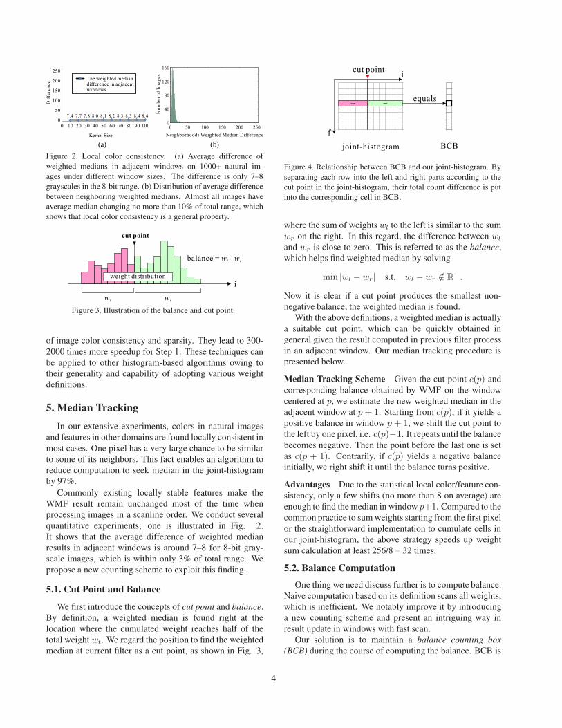
Figure 2. Local color consistency. (a) Average difference ofweighted medians in adjacent windows on 1000+ natural im-ages under different window sizes. The difference is only 7–8grayscales in the 8-bit range. (b) Distribution of average differencebetween neighboring weighted medians. Almost all images haveaverage median changing no more than 10% of total range, whichshows that local color consistency is a general property.

cut point

balance = -w wl r

iweight distribution

wl

wr

Figure 3. Illustration of the balance and cut point.

of image color consistency and sparsity. They lead to 300-2000 times more speedup for Step 1. These techniques canbe applied to other histogram-based algorithms owing totheir generality and capability of adopting various weightdefinitions.

5. Median TrackingIn our extensive experiments, colors in natural images

and features in other domains are found locally consistent inmost cases. One pixel has a very large chance to be similarto some of its neighbors. This fact enables an algorithm toreduce computation to seek median in the joint-histogramby 97%.

Commonly existing locally stable features make theWMF result remain unchanged most of the time whenprocessing images in a scanline order. We conduct severalquantitative experiments; one is illustrated in Fig. 2.It shows that the average difference of weighted medianresults in adjacent windows is around 7–8 for 8-bit gray-scale images, which is within only 3% of total range. Wepropose a new counting scheme to exploit this finding.

5.1. Cut Point and Balance

We first introduce the concepts of cut point and balance.By definition, a weighted median is found right at thelocation where the cumulated weight reaches half of thetotal weight wt. We regard the position to find the weightedmedian at current filter as a cut point, as shown in Fig. 3,

joint-histogram BCB

cut point

+

i

f

equals

Figure 4. Relationship between BCB and our joint-histogram. Byseparating each row into the left and right parts according to thecut point in the joint-histogram, their total count difference is putinto the corresponding cell in BCB.

where the sum of weights wl to the left is similar to the sumwr on the right. In this regard, the difference between wl

and wr is close to zero. This is referred to as the balance,which helps find weighted median by solving

min |wl − wr | s.t. wl − wr /∈ R−.

Now it is clear if a cut point produces the smallest non-negative balance, the weighted median is found.

With the above definitions, a weighted median is actuallya suitable cut point, which can be quickly obtained ingeneral given the result computed in previous filter processin an adjacent window. Our median tracking procedure ispresented below.

Median Tracking Scheme Given the cut point c(p) andcorresponding balance obtained by WMF on the windowcentered at p, we estimate the new weighted median in theadjacent window at p + 1. Starting from c(p), if it yields apositive balance in window p + 1, we shift the cut point tothe left by one pixel, i.e. c(p)−1. It repeats until the balancebecomes negative. Then the point before the last one is setas c(p + 1). Contrarily, if c(p) yields a negative balanceinitially, we right shift it until the balance turns positive.

Advantages Due to the statistical local color/feature con-sistency, only a few shifts (no more than 8 on average) areenough to find the median in window p+1. Compared to thecommon practice to sum weights starting from the first pixelor the straightforward implementation to cumulate cells inour joint-histogram, the above strategy speeds up weightsum calculation at least 256/8 = 32 times.

5.2. Balance Computation

One thing we need discuss further is to compute balance.Naive computation based on its definition scans all weights,which is inefficient. We notably improve it by introducinga new counting scheme and present an intriguing way inresult update in windows with fast scan.

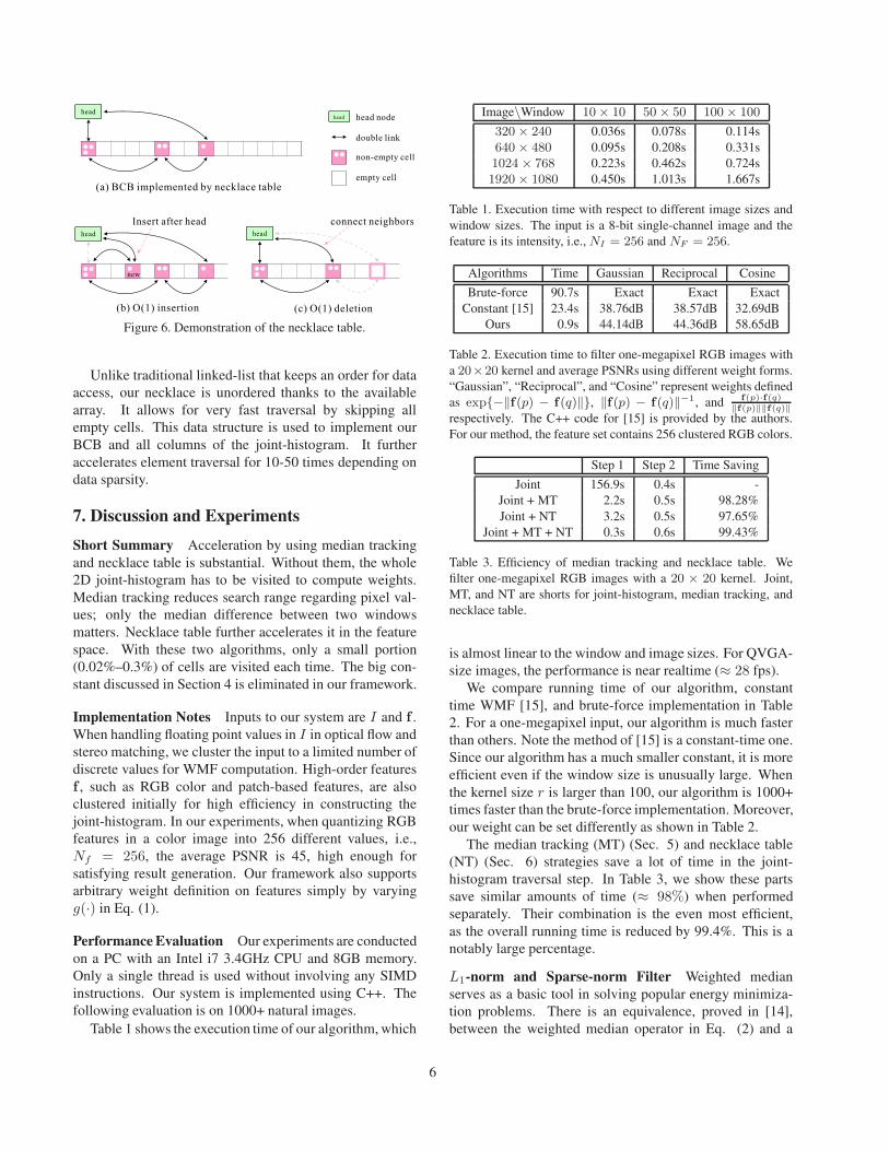
Our solution is to maintain a balance counting box(BCB) during the course of computing the balance. BCB is

4

a 1D array B of NF cells – the same size of columns in ourjoint histogram. As shown in Fig. 4, the f -th cell recordsthe difference of pixel numbers on the two sides of thecut point in the corresponding row of the joint-histogram.Formally, the f -th cell B(f) is constructed as

B(f) = #{q ∈ R(p)|I(q) <= c, f(q) = ff}−#{r ∈ R(p)|I(r) > c, f(r) = ff}, (5)

where c is the cut point location. B(f) measures imbalanceof pixel numbers with regard to feature ff on two sides of c.

Understanding BCB B is very important in our system.It indicates how pixels distribute in the two sides of the cutpoint for each weight because wpq is completely determinedby f(q) when p is the filter center. In WMF computation, thecut point could vary even for adjacent windows that overlapa lot. But BCB makes it possible to re-calculate the balancein the new window quickly, even without needing to knowthe detailed weight for each pixel. This is a fascinating step,as a number of operations to scan data are saved naturally.

With BCB, the balance b in a window can be obtained as

b =Nf−1∑

f=0

B(f) g(ff , f(p)). (6)

This simple expression brings us a brand new way tocalculate weighted median. That is, instead of cumulatingweights, which is costly, we can calculate a lightweightbalance measure counting pixel number difference. It is suf-ficient to tell if the weighted median is found. Specifically,if b is negative, we not only know the cut point c is wrong,but also get the idea in which direction we should move c.Corresponding conclusion can be reached for positive b.

BCB Algorithm In our joint-histogram framework, wemaintain and update BCB as well as the cut point as follows.

1. Initially, we set the cut point to 0, and initialize BCBby counting pixels for each row of the joint-histogram.

2. We seek median by shifting the cut point and checkingthe balance in Eq. (6). This process is the same asthe median tracking scheme presented in Section 5.1.Every time the cut point shifts, we update BCB basedon the joint-histogram.

3. To process a new window largely overlapped withthe current one, we update BCB by only examiningexiting/entering pixels, using only a small number ofplus and minus operations.

This algorithm avoids traversing the joint-histogram forcomputing all weights. It also captures the key propertiesof weighted median. The employment of the cut point, bal-ance, and BCB simplifies computation a lot as mentionedabove.

-6000

-4000

-2000

0

2000

4000

6000

8000

intensity

feat

ure

index

50 100 150 200 250

50

100

150

200

250 0

500

1000

1500

feat

ure

index

50

100

150

200

250

(a) Joint-histogram (b) BCB

Figure 5. Data sparsity in joint-histogram (a) and BCB (b) for theexample shown in Fig. 1(a). A very small number of cells containnon-zero values. Features used here are 256 clustered colors of theimage. We explain it in Sec. 7.

6. Necklace TableIn addition to above algorithms, we also exploit the

sparsity of data distributions for WMF in our new struc-tures. When constructing the joint-histogram and BCB, italways happens that 90%-98% bins/cells are empty in ourquantitative evaluation. It means traversing these elementswastes time. Fig. 5 shows an example.

In this section, we present another data structure callednecklace table. It is a counting table enabling fast traversal.It supports very fast operators as

• O(1) data access;• O(1) element insertion;• O(1) element deletion;• O(N) traversal where N is the non-empty cell number.

Note these four fast operations cannot be achieved simul-taneously by array or linked-list. Our data structure iscomposed of two parts. They are

• counting array that is accessed instantly by index and• necklace, which is an unordered double-linked cycle

built on the counting array for non-empty cells.

One necklace-table example built on our BCB is shown inFig. 6(a). Each cell can be accessed randomly by index.But when the goal is to traverse all non-empty cells, thenecklace can achieve sequential access. The necklace inthis array is initialized as a self-linked head node. Two linksare established for each non-empty cell pointing to previousand next elements.

The above mentioned operations are realized followingthe example in Fig. 6(b) & (c). Data access and traversalare straightforward. For element insertion, we can instantlyaccess the array and update the count. If the cell is emptyoriginally, we insert it to the necklace between the head andits next element. Element deletion reverts this process.

5

(b) nsertionO(1) i (c) O(1) deletion

head

(a) BCB implemented by necklace table

connect neighborshead

Insert after headhead

new

head head node

double link

non-empty cell

empty cell

Figure 6. Demonstration of the necklace table.

Unlike traditional linked-list that keeps an order for dataaccess, our necklace is unordered thanks to the availablearray. It allows for very fast traversal by skipping allempty cells. This data structure is used to implement ourBCB and all columns of the joint-histogram. It furtheraccelerates element traversal for 10-50 times depending ondata sparsity.

7. Discussion and Experiments

Short Summary Acceleration by using median trackingand necklace table is substantial. Without them, the whole2D joint-histogram has to be visited to compute weights.Median tracking reduces search range regarding pixel val-ues; only the median difference between two windowsmatters. Necklace table further accelerates it in the featurespace. With these two algorithms, only a small portion(0.02%–0.3%) of cells are visited each time. The big con-stant discussed in Section 4 is eliminated in our framework.

Implementation Notes Inputs to our system are I and f .When handling floating point values in I in optical flow andstereo matching, we cluster the input to a limited number ofdiscrete values for WMF computation. High-order featuresf , such as RGB color and patch-based features, are alsoclustered initially for high efficiency in constructing thejoint-histogram. In our experiments, when quantizing RGBfeatures in a color image into 256 different values, i.e.,Nf = 256, the average PSNR is 45, high enough forsatisfying result generation. Our framework also supportsarbitrary weight definition on features simply by varyingg(·) in Eq. (1).

Performance Evaluation Our experiments are conductedon a PC with an Intel i7 3.4GHz CPU and 8GB memory.Only a single thread is used without involving any SIMDinstructions. Our system is implemented using C++. Thefollowing evaluation is on 1000+ natural images.

Table 1 shows the execution time of our algorithm, which

Image\Window 10 × 10 50 × 50 100 × 100

320 × 240 0.036s 0.078s 0.114s640 × 480 0.095s 0.208s 0.331s1024 × 768 0.223s 0.462s 0.724s1920 × 1080 0.450s 1.013s 1.667s

Table 1. Execution time with respect to different image sizes andwindow sizes. The input is a 8-bit single-channel image and thefeature is its intensity, i.e., NI = 256 and NF = 256.

Algorithms Time Gaussian Reciprocal CosineBrute-force 90.7s Exact Exact Exact

Constant [15] 23.4s 38.76dB 38.57dB 32.69dBOurs 0.9s 44.14dB 44.36dB 58.65dB

Table 2. Execution time to filter one-megapixel RGB images witha 20×20 kernel and average PSNRs using different weight forms.“Gaussian”, “Reciprocal”, and “Cosine” represent weights definedas exp{−‖f(p) − f(q)‖}, ‖f(p) − f(q)‖−1, and f(p)·f(q)

‖f(p)‖‖f(q)‖respectively. The C++ code for [15] is provided by the authors.For our method, the feature set contains 256 clustered RGB colors.

Step 1 Step 2 Time SavingJoint 156.9s 0.4s -

Joint + MT 2.2s 0.5s 98.28%Joint + NT 3.2s 0.5s 97.65%

Joint + MT + NT 0.3s 0.6s 99.43%

Table 3. Efficiency of median tracking and necklace table. Wefilter one-megapixel RGB images with a 20 × 20 kernel. Joint,MT, and NT are shorts for joint-histogram, median tracking, andnecklace table.

is almost linear to the window and image sizes. For QVGA-size images, the performance is near realtime (≈ 28 fps).

We compare running time of our algorithm, constanttime WMF [15], and brute-force implementation in Table2. For a one-megapixel input, our algorithm is much fasterthan others. Note the method of [15] is a constant-time one.Since our algorithm has a much smaller constant, it is moreefficient even if the window size is unusually large. Whenthe kernel size r is larger than 100, our algorithm is 1000+times faster than the brute-force implementation. Moreover,our weight can be set differently as shown in Table 2.

The median tracking (MT) (Sec. 5) and necklace table(NT) (Sec. 6) strategies save a lot of time in the joint-histogram traversal step. In Table 3, we show these partssave similar amounts of time (≈ 98%) when performedseparately. Their combination is the even most efficient,as the overall running time is reduced by 99.4%. This is anotably large percentage.

L1-norm and Sparse-norm Filter Weighted medianserves as a basic tool in solving popular energy minimiza-tion problems. There is an equivalence, proved in [14],between the weighted median operator in Eq. (2) and a

6

(b) Ours (2.23s)(a)Xu et al.(7.73s)

(c)Input

Ours

Input

Xu et al.

Figure 7. Our fast WMF can be used as L0-norm filter (α = 0in Eq. (8)) to remove details while preserving large-magnitudestructures better than global minimization [23]. (a) Global mini-mization in 3 iterations uses 7.73s; (b) Our filtering process in 10iterations uses 2.23s.

global energy function defined as

minI∗

∑

q∈R(p)

wpq‖I∗(p) − I(q)‖, (7)

where I∗ is the output image or field. The commonlyemployed L1 minimization expressed by Eq. (7) manifeststhe vast usefulness of weighted median filter.

Further, minimization with higher-sparsity norms Lα

with 0 ≤ α < 1 like

minI∗

∑

q∈R(p)

wpq‖I∗(p) − I(q)‖α, (8)

can also be accomplished in the form of reweighted L1. Thedetails of reweighted L1 were discussed in [3]. Our fastWMF with its weight defined as wpq‖I(p) − I(q)‖α−1 canbe used to solve these functions. We shown in Fig. 7 a L0-norm smoothing result using our WMF method. It betterpreserves structures than the global minimization approachpresented in [23]. Our method speed is higher. More imagefiltering results are put into the project website.

Non-local Regularizer WMF can be taken as a non-local regularizer in different computer vision systems. A

(c) Ours

(b) Sun et al.

(a)Input

Figure 8. Estimating optical flow by our WMF. (a) Input andclose-ups. (b) Result of [19]. (c) Our result by replacing globaloptimization by our local WMF. Our implementation uses onlyRGB color as features. The quality is similar but the running timeis much shortened.

Input

Ours

Figure 9. The watercolor painting effect generated with weightsdefined as Jaccard similarity in RGB color.

common set of optimization problems involving nonlocaltotal variation regularizer can be expressed as

∑

p

∑

q∈R(p)

wpq · ‖I(p) − I(q)‖. (9)

It finds optimal solutions by performing WMF (see [19] formore details). Taking optical flow estimation as an example,our revolutionized WMF shortens running time from theoriginal 850 seconds to less than 30 seconds. Results forone example are shown in Fig. 8.

Varying Weights And Features Not limited to Gaussianweights, our framework can handle arbitrary weight defini-tion based on features. One example is to use RGB color asthe feature and define the weight wpq as a Jaccard similarity[13]:

min(R(p), R(q)) + min(G(p), G(q)) + min(B(p), B(q))max(R(p), R(q)) + max(G(p), G(q)) + max(B(p), B(q))

,

where R(p), G(p), and B(p) are the RGB channels off(p). Even for this special weight, optimal solution can be

7

(a) (b) (c)

(d) (e)

Figure 10. Cross-median filter. (d) and (e) are obtained by filtering(a) with feature maps (b) and (c) respectively. The filter smoothsstructure according to different features, creating the style-transfereffect.

obtained, which generates a watercolor painting effect, asshown in Fig. 9.

Further, our framework supports cross/joint weightedmedian filtering. Thus features of others image can be takenas special guidance. A “style-transfer” example is shown inFig. 10.

8. Concluding Remarks

Weighted median is an inevitable and practical tool infilter and energy minimization for many applications. Wemuch accelerated it in a new framework with several effec-tive techniques. We believe it will greatly profit buildingefficient computer vision systems in different domains.

Acknowledgements

We thank Qiong Yan for the help in coding and algorithmdiscussion. This work is supported by a grant from theResearch Grants Council of the Hong Kong SAR (projectNo. 413110) and by NSF of China (key project No.61133009).

References[1] A. Adams, J. Baek, and M. A. Davis. Fast high-dimensional

filtering using the permutohedral lattice. Computer GraphicsForum, 29(2):753–762, 2010.

[2] A. Adams, N. Gelfand, J. Dolson, and M. Levoy. Gaussiankd-trees for fast high-dimensional filtering. ACM Transac-tions on Graphics (TOG), 28(3):21, 2009.

[3] E. J. Candes, M. B. Wakin, and S. P. Boyd. Enhancingsparsity by reweighted l1 minimization. Journal of FourierAnalysis and Applications, 14(5-6):877–905, 2008.

[4] J. Chen, S. Paris, and F. Durand. Real-time edge-awareimage processing with the bilateral grid. ACM Transactionson Graphics (TOG), 26(3):103, 2007.

[5] D. Cline, K. B. White, and P. K. Egbert. Fast 8-bit medianfiltering based on separability. In Image Processing, 2007.ICIP 2007. IEEE International Conference on, volume 5,pages V–281. IEEE, 2007.

[6] F. Durand and J. Dorsey. Fast bilateral filtering for thedisplay of high-dynamic-range images. ACM Transactionson Graphics (TOG), 21(3):257–266, 2002.

[7] Z. Farbman, R. Fattal, D. Lischinski, and R. Szeliski. Edge-preserving decompositions for multi-scale tone and detailmanipulation. ACM Trans. Graph., 27(3), 2008.

[8] E. S. Gastal and M. M. Oliveira. Domain transform for edge-aware image and video processing. ACM Transactions onGraphics (TOG), 30(4):69, 2011.

[9] E. S. Gastal and M. M. Oliveira. Adaptive manifolds forreal-time high-dimensional filtering. ACM Transactions onGraphics (TOG), 31(4):33, 2012.

[10] K. He, J. Sun, and X. Tang. Guided image filtering. InComputer Vision–ECCV 2010, pages 1–14. Springer, 2010.

[11] T. S. Huang. Two-dimensional digital signal processing II:transforms and median filters. Springer-Verlag New York,Inc., 1981.

[12] M. Kass and J. Solomon. Smoothed local histogram filters.ACM Transactions on Graphics (TOG), 29(4):100, 2010.

[13] M. Levandowsky and D. Winter. Distance between sets.Nature, 234(5323):34–35, 1971.

[14] Y. Li and S. Osher. A new median formula with applicationsto pde based denoising. Commun. Math. Sci, 7(3):741–753,2009.

[15] Z. Ma, K. He, Y. Wei, J. Sun, and E. Wu. Constant timeweighted median filtering for stereo matching and beyond.In ICCV. IEEE, 2013.

[16] S. Paris and F. Durand. A fast approximation of the bilateralfilter using a signal processing approach. In ComputerVision–ECCV 2006, pages 568–580. Springer, 2006.

[17] S. Perreault and P. Hebert. Median filtering in constant time.Image Processing, IEEE Transactions on, 16(9):2389–2394,2007.

[18] F. Porikli. Constant time o (1) bilateral filtering. In ComputerVision and Pattern Recognition, 2008. CVPR 2008. IEEEConference on, pages 1–8. IEEE, 2008.

[19] D. Sun, S. Roth, and M. J. Black. Secrets of optical flowestimation and their principles. In Computer Vision andPattern Recognition (CVPR), 2010 IEEE Conference on,pages 2432–2439. IEEE, 2010.

[20] C. Tomasi and R. Manduchi. Bilateral filtering for gray andcolor images. In Computer Vision, 1998. Sixth InternationalConference on, pages 839–846. IEEE, 1998.

[21] B. Weiss. Fast median and bilateral filtering. ACM Transac-tions on Graphics (TOG), 25(3):519–526, 2006.

[22] L. Xu, C. Lu, Y. Xu, and J. Jia. Image smoothing via L0gradient minimization. ACM Trans. Graph., 30(6), 2011.

[23] L. Xu, Q. Yan, Y. Xia, and J. Jia. Structure extraction fromtexture via relative total variation. ACM Transactions onGraphics (TOG), 31(6):139, 2012.

[24] Q. Yang, K.-H. Tan, and N. Ahuja. Real-time o (1) bilateralfiltering. In Computer Vision and Pattern Recognition, 2009.CVPR 2009. IEEE Conference on, pages 557–564. IEEE,2009.

8