10. Urban Image Classification: Per-pixel Classifiers, Sub ... · 1 10. Urban Image Classification:...
42
1 10. Urban Image Classification: Per-pixel Classifiers, Sub-pixel Analysis, Object-based Image Analysis, and Geospatial Methods Soe W. Myint 1 , Victor Mesev 2 , Dale Quattrochi 3 , and Elizabeth A. Wentz 1 1 School of Geographical Sciences and Urban Planning, Arizona State University, Coor Hall, 5th floor, 975 S. Myrtle Ave., Tempe, AZ 85287, USA 2 Department of Geography, Florida State University, 323 Bellamy Building, 113 Collegiate Loop, Tallahassee, FL 32306-2190, USA 3 Earth Science Office, NASA Marshall Space Flight Center, Huntsville, AL 35812, USA *Author to whom correspondence should be addressed: E-Mail: [email protected] Keywords: urban classification, per-pixel, sub-pixel, object-based, geospatial. CONTENTS 1.0 Introduction 2.0 Remote sensing methods for urban classification and interpretation 2.1 Per-pixel methods 2.2 Sub-pixel methods 2.3 Object-based methods https://ntrs.nasa.gov/search.jsp?R=20140012911 2018-08-01T02:56:47+00:00Z
Transcript of 10. Urban Image Classification: Per-pixel Classifiers, Sub ... · 1 10. Urban Image Classification:...

1
10. Urban Image Classification: Per-pixel Classifiers, Sub-pixel
Analysis, Object-based Image Analysis, and Geospatial Methods
Soe W. Myint1, Victor Mesev2, Dale Quattrochi3, and Elizabeth A. Wentz1
1 School of Geographical Sciences and Urban Planning, Arizona State University, Coor Hall, 5th
floor, 975 S. Myrtle Ave., Tempe, AZ 85287, USA
2 Department of Geography, Florida State University, 323 Bellamy Building, 113 Collegiate
Loop, Tallahassee, FL 32306-2190, USA
3 Earth Science Office, NASA Marshall Space Flight Center, Huntsville, AL 35812, USA
*Author to whom correspondence should be addressed: E-Mail: [email protected]
Keywords: urban classification, per-pixel, sub-pixel, object-based, geospatial.
CONTENTS
1.0 Introduction
2.0 Remote sensing methods for urban classification and interpretation
2.1 Per-pixel methods
2.2 Sub-pixel methods
2.3 Object-based methods
https://ntrs.nasa.gov/search.jsp?R=20140012911 2018-08-01T02:56:47+00:00Z

2
2.4 Geospatial methods
3.0 Concluding remarks
4.0 References
1.0 Introduction
Remote sensing methods used to generate base maps to analyze the urban environment rely
predominantly on digital sensor data from space-borne platforms. This is due in part from new
sources of high spatial resolution data covering the globe, a variety of multispectral and
multitemporal sources, sophisticated statistical and geospatial methods, and compatibility with
GIS data sources and methods. The goal of this chapter is to review the four groups of
classification methods for digital sensor data from space-borne platforms; per-pixel, sub-pixel,
object-based (spatial-based), and geospatial methods. Per-pixel methods are widely used
methods that classify pixels into distinct categories based solely on the spectral and ancillary
information within that pixel. They are used for simple calculations of environmental indices
(e.g., NDVI) to sophisticated expert systems to assign urban land covers (Stefanov et al., 2001).
Researchers recognize however, that even with the smallest pixel size the spectral information
within a pixel is really a combination of multiple urban surfaces. Sub-pixel classification
methods therefore aim to statistically quantify the mixture of surfaces to improve overall
classification accuracy (Myint, 2006a). While within pixel variations exist, there is also
significant evidence that groups of nearby pixels have similar spectral information and therefore
belong to the same classification category. Object-oriented methods have emerged that group
pixels prior to classification based on spectral similarity and spatial proximity. Classification
accuracy using object-based methods show significant success and promise for numerous urban

3
applications (Myint et al., 2011). Like the object-oriented methods that recognize the importance
of spatial proximity, geospatial methods for urban mapping also utilize neighboring pixels in the
classification process. The primary difference though is that geostatistical methods (e.g., spatial
autocorrelation methods) are utilized during both the pre- and post-classification steps (Myint
and Mesev, 2012).
Within this chapter, each of the four approaches is described in terms of scale and accuracy
classifying urban land use and urban land cover; and for its range of urban applications. We
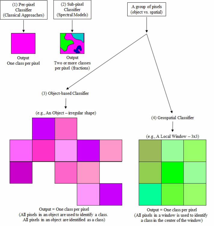
demonstrate the overview of four main classification groups in Figure 1 while Table 1 details the
approaches with respect to classification requirements and procedures (e.g., reflectance
conversion, steps before training sample selection, training samples, spatial approaches
commonly used, classifiers, primary inputs for classification, output structures, number of output
layers, and accuracy assessment). The chapter concludes with a brief summary of the methods
reviewed and the challenges that remain in developing new classification methods for improving
the efficiency and accuracy of mapping urban areas.
Insert Figure 1 here
Insert Table 2
2.0 Remote sensing methods for urban classification and interpretation
Urban areas are comprised of a heterogeneous patchwork of land covers and land uses that are
juxtaposed so that classification of specific classes using remote sensing data can be problematic.
Derivation of classification methods for urban landscape features has evolved in tandem with

4
increasing spatial, spectral, and temporal resolutions of remote sensing instruments (e.g., from 90
m Landsat Multispectral Scanner-MSS to 30 m to the Landsat Enhanced Thematic Mapper Plus
[ETM+] and Operational Land Imager [OLI] data and progressing to sub-meter spatial resolution
products available from commercial systems such as .34 m Geoeye) to achieve more robust
digital classification schemes. This evolution of classification techniques, however, does not
imply that one method is better than another. As with the type of satellite remote sensing data
that are employed for analyses, the application of a specific algorithm for classification of urban
land cover and land use is dependent upon what the user’s objectives are, and what level of
detail, frequency, and sensors are required for the anticipated or resulting output products. Table
2 shows urban remote sensing applications with regards to spatial, temporal, and sensor
resolutions.
2.1 Per-pixel methods
Scale is indelible when conducting per pixel classifications. The spatial resolution of the sensor
dictates the classification type, range, and accuracy of urban land use and urban land cover. That
is because individual urban features are rarely the same size as pixels, nor are they conveniently
rectangular in shape. Add temporal scale representing rapid urban activity and per pixel
classifications become even more removed from reality. Refining the spatial resolution and
reducing the area of the pixel does not necessarily lead to improvements in classification
accuracy, and may even introduce additional spectral noise, especially when pixels are smaller
than urban features. In all, the ideal situation that each pixel can be identified to represent
conclusively one and only one land cover type has now long been abandoned. So too the perfect

5
relationship between the pixel and the field-of-view, which assumes reflectance is recorded
entirely and uniformly from within the spatial limits of individual pixels (Figure 1).
Regardless, the appeal of per-pixel or hard classifications remains; predominantly because they
produce crisp and convenient thematic coverages that can be easily integrated with raster-based
GIS models (Table 1). Composite models and methodologies containing information from
remotely sensed sources are critical for revising databases and for producing comprehensive
query-based urban applications. To preserve this relationship with GIS, the quality of per-pixel
classifications must be monitored not only using conventional determination of accuracy based
on comparisons with more reliable reference data, but also in relation to levels of suitability or
‘scale of appropriateness.’ Both were evident in the USGS hierarchical scheme (Anderson et al.,
1976) using the much-cited 85% as a general guideline for the accuracy of urban features, and
which subsequently established a benchmark for researchers to attain and supersede using a
variety of statistical and stochastic per-pixel techniques. Some of these focused exclusively on
maximizing computational class separability, using the traditional maximum likelihood
algorithm (Strahler 1980) and the more recent support vector machines (Yang, 2011), while
others developed methodologies that imported extraneous information when aggregating
spectrally similar pixels (Mesev, 1998), by incorporating contextual relationships (Stuckens et
al., 2000), or by measuring pixel inter-connectivity (Barr and Barnsley, 1997). In both,
classification accuracy typically improves only marginally, simply because there is an inherent
numerical limitation to the extent individual pixel values can comprehensively represent the
multitude of true urban features within the rigid confines of their regular-sized pixel limits
(Fisher, 1997).
6
However within these numerical limits per-pixel classification accuracy can be consistently high
if the appropriate spatial resolution (i.e., pixel size) is identified with respect to the suitable level
of urban detail (Table 2). Such ideas of scale appropriateness can be traced back to Welch
(1982), and have since been widely accepted as an important part of the class training process.
But the decision is far from trivial, and must also consider the appropriate scale of analysis
(Mesev, 2012). Consider a continuous scale that can be conceptualized by levels of measurement
from remote sensor data; ranging from the representation of atomistic urban features (building,
tree, sidewalk, etc.) at the micro scale, to the representation of aggregate urban features
(residential neighborhoods, industrial zones, or even complete urban areas) at the macro scale.
Micro urban remote sensing by per-pixel classification remains highly tenuous (even using meter
and sub meter resolutions from the latest sensors) and any reliable interpretation is extracted
directly from the spatial orientation of pixels—in a similar vein to conventional interpretation of
aerial photography, but with lower clarity and with limited stereoscopic capabilities. However,
the spectral heterogeneity problem is less restrictive at the macro scale of analysis where
classified pixels, instead of measuring individual urban objects, can be aggregated to represent a
generalized view of urban areas, including total imperviousness, approximate lateral growth, and
overall greenness. It is at this scale of analysis that many types of urban processes, such as
sprawl, congestion, poverty, land use zoning, storm water flow, and heat islands, can be studied
simultaneously across an entire urban area as part of the search for theories of livability and
sustainability. In sum, per-pixel classifications produce simple and convenient thematic maps of
urban land use and land cover that can be incorporated into GIS models. The spatial resolution of
the remote sensor, however, limits their accuracy away from mapping individual urban features
7
with any level of pragmatic precision and towards more traditional macro scales of generalized
land cover combinations reminiscent of the timeless V-I-S model (Ridd, 1995).
Insert Table 2 here
2.2 Sub-pixel methods
If locational and thematic accuracy of urban representation from remote sensing is paramount,
per-pixel classifications can be modified statistically to measure spectral mixtures representing
multiple land cover classes within individual pixels. These are termed sub-pixel algorithms or
soft classifications because pixels are no longer constrained to representing single classes, but
instead represent various proportions of land cover classes which are conceptually more akin to
the spatial and compositional heterogeneity of urban configurations (Ji and Jensen, 1999; Small,
2004). The debate on which approach, per-pixel or sub-pixel, can again be tied to the scale of
urban analysis. For example, the measurement of impervious surfaces is particularly amenable to
sub-pixel classification because pixels can represent a continuum of imperviousness, from total
coverage (downtown areas and industrial estates) to scant dispersion intermingled with bio-
physical land covers (city parks). Extensive research has been devoted to more precise
quantification of impervious surfaces, and other urban land covers at sub-pixel level, such as
linear mixture models (Wu and Murray, 2003; Rashed, et al., 2003), background removal
spectral mixture analysis (Ji and Jensen, 1999; Myint, 2006a), Bayesian probabilities (Foody et
al., 1992; Mesev, 2001; Eastman and Laney, 2002; Hung and Ridd, 2002), artificial neural
network (Foody and Aurora, 1996; Zhang and Foody, 2001), normalized spectral mixture
analysis (Wu and Yuan, 2007; Yuan and Bauer, 2007), fuzzy c-means methods (Fisher and

8
Pathirana, 1990; Foody 2000), multivariate statistical analysis (Bauer et al., 2004; Yang and Liu,
2005; Bauer et al., 2007), and regression trees (Yang et al., 2003a and 2003b; Homer et al.,
2007).
Among these, linear spectral mixture analysis, regression analysis, and regression trees have had
a wider appeal because they are theoretically and computationally simpler, as well as more
prevalent in many commercial software packages. However, the success of measuring urban land
cover types using linear techniques is dependent on identifying spectrally-pure endmembers,
preferably using reference samples collected in the field (Adams et al., 1995; Roberts et al., 1998
and 2012). Although Weng and Hu (2008) derived moderate accuracy levels from employing
linear spectral mixture analysis using ASTER and Landsat ETM+ sensor imagery, they
discovered that artificial neural networks were also capable of performing non-linear mixing of
land cover types at the sub-pixel level (Borel and Gerstl, 1994; Ray and Murray, 1996). Another
limitation with linear spectral mixture classifiers is that they do not permit the number of
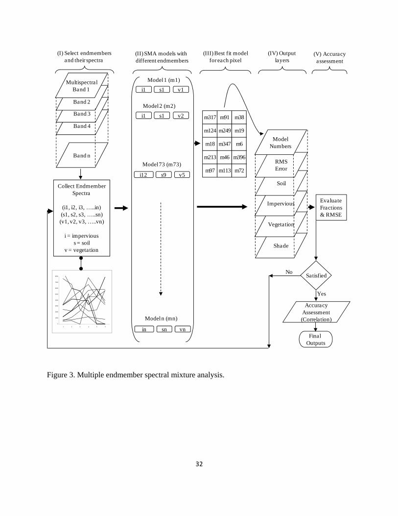
endmembers to be greater than the number of spectral bands (Myint, 2006a). In response, a
multiple endmember spectral mixture analysis (MESMA) has been developed to identify many
more endmember types to represent the heterogeneous mixture of urban land cover types
(Rashed et al., 2003; Powell et al., 2007; Myint and Okin, 2009). Diagrams demonstrating linear
spectral mixture analysis and multiple endmember spectral mixture analysis are provided in
Figures 2 and 3 respectively.
Figure 2 here
Figure 3 here

9
Two challenges dominate the research efforts to improve subpixel analysis methods for urban
settings. The first challenge is pixel size. Identifying endmembers for all classes in images with
large to medium pixels in urban areas is difficult given the heterogeneous nature of urban areas.
In small spatial distances (e.g., < 30 m), surfaces rapidly change from impervious, to grass, to
building. The smaller pixel size (e.g., 1m or submeter), however, is not always the optimal
solution. While pixels may not reflect a mixture of the desired endmembers (e.g., a combination
of asphalt and grass), reflectance from unwanted features begin to appear that need to be filtered
(e.g., oil surfaces and automobiles in asphalt; chimneys and air conditions on rooftops). The
second limitation is that it is almost impossible to identify all possible endmembers in a study
area and classification accuracy can be degraded by the potential presence of unknown classes or
unidentified classes (e.g., the asphalt and rooftop examples from above). This is because the
classifier is based on the assumption that the sum of the fractional proportions of all possible
endmembers in a pixel is equal to one. Although this type of modeling is conceptually more
representative of urban land cover, from a practical standpoint it nonetheless perpetuates the
mixed pixel problem and presents thematic and semantic limitations to urban land classification
schemes. In other words, output from sub-pixel analysis produces fractional classes that are more
difficult to integrate with GIS data and may even limit their portability for comparisons across
space and through time.
2.3 Object-based methods
With the representational limitations of purely spectrally-based per-pixel and sub-pixel
classifications it was only a matter of time before the shift to the spatial domain gained

10
momentum. Even from a purely intuitive standpoint finer resolution (i.e., smaller pixels or large
cartographic-scale) imagery exhibit higher levels of detailed features that mimic the
heterogeneous nature of urban areas. This greater level of spatial detail invariably also leads to
many more uncertain spectral classes–known as noise–which can be true but potentially
unwanted urban features such as chimneys or manhole covers. Assuming spectral noise is
reduced, images with spatial resolutions ranging from about 0.25 to 5 m have the potential to
help identify urban structures necessary to perform many urban applications, including
estimation of population based on the number of dwellings of different housing types, residential
water use, predicting energy consumption, urban heat island, outdoor water use, solar energy use,
and storm water pollution modeling (Jensen and Cowen, 1999).
Conceptually, spatial or object-based approaches are most applicable to high spatial resolution
remote sensing data, where objects of interest are larger than the ground resolution element, or
pixel. Urban objects may be vegetated features of urban landscapes (e.g., trees, shrubs, golf
course) or anthropogenic features (e.g., buildings, pools, sidewalks, roads, canals). With regards
to mapping categorical data or identifying land use land cover classes, remotely sensed image
analysis started to shift from pixel-based (per-pixel) to object based image analysis (OBIA) or
geospatial object based image analysis (GEOBIA) around the year 2000 (Blaschke T., 2010).
The object-centered classification prototype starts with the generation of segmented objects at
multiple scales (Desclee, et al., 2006; Navulur, 2007; Im et al., 2008; Myint et al., 2008). To
demonstrate, Walker and Briggs (2007) employed an object-oriented classification procedure to
effectively delineate woody vegetation in an arid urban ecosystem using high spatial resolution
true-color aerial photography (without the near infrared band) and achieved an overall accuracy

11
of 81%. Hermosilla et al. (2012) developed two object-based approaches for automatic building
detection and localization using high spatial resolution imagery and LiDAR data. Stow et al
(2007) further developed object-based classification by taking advantage of the spatial frequency
characteristics of multispectral data, and then measuring the proportions of vegetation,
imperviousness, and soil sub-objects to identify residential land use in Accra, Ghana (they
documented an overall accuracy of 75%). In another study by Zhaou et el (2008), post-
classification change detection based on the object-based analysis of multitemporal high spatial
resolution produced even higher accuracies of 92% and 94%; while Myint and Stow (2011)
demonstrated the effectiveness of object-based strategies based on decision rules (i.e.,
membership functions) and nearest neighbor classifiers on high spatial resolution Quickbird
multispectral satellite data over the city of Phoenix. These are further supported by Myint et al.
(2011) who directly compared the accuracy from object-based classifications (90%) with more
traditional spectral-based classifications (68%). The land-cover classes that the authors identified
for this particular study include buildings, other impervious surfaces (e.g., roads and parking
lots), unmanaged soil, trees/shrubs, grass, swimming pools, and lakes/ponds. The study selected
500 samples points that led to approximately 70 points per class (7 total classes) using a stratified
random sampling approach for the accuracy assessment of two different subsets of QuickBird
over Phoenix. To be consistent and for precise comparison purposes, they applied the same
sample points generated for the output generated by the objectbased classifier as the output
produced by the traditional classification technique (i.e., maximum likelihood).
In general, spectrally similar signatures such as dark/gray soil, dark/gray rooftops, dark/gray
roads, swimming pools/blue color rooftops, and red soil/red rooftop remain problematic even
12
with object-based approaches. Furthermore, the most commonly used object-oriented software
(Definiens or eCognition) is required to perform a tremendous number of segmentations of
objects from all spectral bands using various scale parameters. There is no universally accepted
method to determine an optimal level of scale (e.g., object size) to segment objects, and a single
scale may not be suitable for all classes. The most feasible approach may be to select the bands
for membership functions at the scale that identifies the class with variable options and analyze
them heuristically on the display screen. Given that the nearest neighbor classifier and decision
rule available in the object-based approach are non-parametric approaches, they are independent
of the assumption that data values need to be normally distributed. This is advantageous, because
most data are not normally distributed in many real world situations. Another advantage of the
object-based approach is that it allows additional selection or modification of new objects
(training samples) at iterative stages, until the satisfactory result is obtained. However, the
object-based approach has a significant problem when dealing with a remotely sensed data over a
fairly large area since computer memory needs to be used extensively to segment tremendous
numbers of objects using multispectral bands. This is true even for fine spatial resolution data
with fewer bands (e.g., QuickBird) over a small study area when requiring smaller scale
parameters (smaller objects). Figure 4 shows segmented images at scale level 25, 50, and 100
using a subset of a QuickBird image over Phoenix. Figure 5 demonstrates how hierarchical
image segmentation delineates image objects at various scales.
Figure 4 here
Figure 5 here

13
2.4 Geospatial methods
Texture plays an important role in the human visual system for pattern recognition and
interpretation. For image interpretation, pattern is defined as the overall spatial form of related
features, where the repetition of certain forms is a characteristic pattern found in many cultural
objects and some natural features. Local variability in remotely sensed data, which is part of
texture or pattern analysis, can be characterized by computing the statistics of a group of pixels,
e.g., standard deviation, coefficient of variance or autocovariance, or by the analysis of fractal
similarities or autocorrelation of spatial relationships. There have been some attempts to improve
the spectral analysis of remotely sensed data by using texture transforms in which some measure
of variability in digital numbers is estimated within local windows; e.g. the contrast between
neighboring pixels (Edwards et al., 1988), standard deviation (Arai, 1993), or local variance
(Woodcock and Harward, 1992). One commonly used statistical procedure for interpreting
texture uses an image spatial co-occurrence matrix, which is also known as a gray level co-
occurrence matrix (GLCM) (Franklin et al., 2000). There are a number of texture measures,
which could be applied to spatial co-occurrence matrices for texture analysis (Peddle and
Franklin, 1991). For instance, Herold et al. (2003) proposed a method based on using landscape
metrics to classify IKONOS sensor images, which in turn is compared to a GLCM. Liu et al.
(2006) further contrasted spatial metrics, GLCM, and semi-variograms in terms of urban land
use classification.
Lam et al. (1998) demonstrated how fractal dimensions yield quantitative insight into the spatial
complexity and information contained in remotely sensed data. Quattrochi et al. (1997) went
further and created a software package known as the Image Characterization and Modeling

14
System (ICAMS) to explore how the fractal dimension is related to surface texture. Fractal
dimensions were also analyzed by Emerson et al. (1999) who used the isarithm method and
Moran’s I and Geary’s C spatial autocorrelation measures to observe the differing spatial
structure of the smooth and rough surfaces in remotely sensed images. In terms of other
geospatial techniques, De Jong and Burrough (1995) and Woodcock et al (1988) implemented
variograms to measurements derived from remotely sensed to quantitatively describe urban
spatial patterns. Myint and Lam (2005a; 2005b) and Myint et al. (2006) developed a number of
lacunarity approaches to characterize urban spatial features with completely different texture
appearances that may share the same fractal dimension values. Both studies report that lacunarity
can be considered more effective in comparison to fractal approaches for urban mapping.
The geospatial methods described so far may not provide satisfactory accuracies when they are
applied to the classification of urban features from fine spatial resolution remotely sensed
images. That is mainly because most of them focus primarily on coupling features and objects at
a single scale and cannot determine the effective representative value of particular texture
features according to their directionality, spatial arrangements, variations, edges, contrasts, and
the repetitive nature of object and features. There have been a number of reports in spatial
frequency analysis of mathematical transforms, which provide solutions using multi-resolution
analysis. Recent developments in spatial/frequency transforms such as the Fourier transform,
Wigner distribution, discrete cosine transform, and wavelet transform have all provided sound
multi-resolution analytical tools (Bovik et al., 1990; Zhu and Yang, 1998).

15
Of all transformation approaches, wavelets play the most critical part in texture analysis.
Wavelets are part of spatial and frequency based classification approaches, and a local window
plays an important role in measuring and characterizing spatial arrangements of objects and
features. Homogeneity, size of regions, characteristic scale, directionality, and spatial periodicity
are important issues that should be considered to identify local windows when performing
wavelet analysis (Myint, 2010). From a computational perspective, the ideal window size is the
smallest size that also produces the highest accuracy (Hodgson, 1998). The accuracy should
increase with a larger local window size since it contains more information than a smaller
window size and therefore provides more complete coverage of spatial variation, directionality
and spatial periodicity of a particular texture. However, minimization of local window size is
also important in spatial-based urban image classification techniques since a larger window size
tends to cover more urban land cover features and consequently creates mixed boundary pixels
or mixed land cover problems. However, some spatial and frequency approaches such as wavelet
dyadic decomposition approaches require large window sizes to capture spatial information at
multiple scales (Myint, 2006b). The potential solution to this problem would be to employ a
multi-scale overcomplete wavelet analysis using an infinite scale decomposition procedure. This
is because a large spatial coverage or a large local window is not needed to describe a spatial
pattern. Furthermore, this approach can measure different directional information of anisotropic
features at unlimited scales, and it is designed to normalize and select effective features to
identify urban classes. Myint and Mesev (2012) employed a wavelet-based classification method
to identify urban land use and land cover classes using different decision rule sets and spatial
measures and demonstrated the effectiveness of wavelets. However, the current wavelet-based
classification system with the dyadic wavelet approach is limited by the fact that higher-level

16
sub-images are just a quarter of the preceding image. In general, smaller window size is
generally thought to yield higher accuracy in geospatial-based image classification because if the
window is too large, much spatial information from two or more land cover classes could create
a mixed boundary problem. Further research is required to consider an overcomplete wavelet
approach that can generate spatial arrangements of objects and features at any scale level for
urban mapping. Such an approach could potentially be applicable to any land use/ land cover
system at any resolution or scale because it can effectively use any window size. Figure 6 shows
how wavelet approaches work in comparison to other geospatial approaches in urban mapping.
Figure 6 here
3.0 Concluding remarks
Interpreting urban land cover from data captured by remote sensors remains a conceptual and
technical challenge. Accuracy levels are typically lower than the interpretation of more naturally-
occurring surfaces. However, huge strides have been made with the formulation of statistical
models that help disentangle the spectral and spatial complexity of urban land covers. Whereas
per-pixel classification have stood the test of time (primarily for pragmatic reasons, especially
when integrated with GIS-handled datasets), developments in sub-pixel, object-based and
geospatial techniques have begun, at last, to reproduce the geographical configuration and
compositional texture of urban structures. These developments are further tempered by
conceptual developments that now consider the “appropriateness” of scale (understanding the
level of urban structural measurements) and the “appropriateness” of time (understanding the lag
between urban process and urban structure). Both are critical for measuring the rate of urban

17
change; not simply the amount of lateral growth, but also the juxtaposition of land use within
existing urban limits. Further research will only improve our use of remote sensor data for
measuring urban patterns and in turn will complement our understanding of key urban processes.

18
4.0 References:
Adams, J. B., Sabol, D. E., Kapos, V., Almeida-Filho, R., Roberts, D. A., Smith, M. O. &
Gillespie, A.R. 1995. Classification of multiple images based on fractions of endmembers:
application to landcover change in the Brazilian Amazon, Remote Sensing of Environment, 52,
137–154.
Anderson, J. R., Hardy, E. E., Roach, J. T. and Witmer, R. E. 1976. A land use and land cover
classification system for use with remote sensor data. U.S. Geological Survey Professional
Paper, 964. http://landcover.usgs.gov/pdf/anderson.pdf.
Arai, K., 1993. A classification method with a spatial-spectral variability. International Journal
of Remote Sensing, 14, 699-709.
Barr, S., & Barnsley, M. A., 1997. A region-based, graph-theoretic data model for the inference
of second-order thematic information from remotely-sensed images. International Journal of
Geographical Information Science, 11, 555-576.
Bauer, M. E., Heinert, N. J., Doyle, J. K., & Yuan, F. 2004. Impervious surface mapping and
change monitoring using satellite remote sensing, Proceedings of the ASPRS 2004 Annual
Conference, 24-28 May, Denver, Colorado.
Bauer, M. E., Loeffelholz, B. C., & Wilson, B. 2007. Estimating and mapping impervious
surface area by regression analysis of Landsat imagery. In Q. Wang (Ed.), Remote Sensing of
Impervious Surfaces, pp. 3-20. Boca Raton, Florida: CRC Press.
19
Blaschke T. 2010. Object-based image analysis for remote sensing. ISPRS International Journal
of Photogrammetry and Remote Sensing, 65, 2–16.
Borel, C. C., & Gerstl, S. A. W. 1994. Nonlinear spectral mixing models for vegetative and soil
surfaces, Remote Sensing of Environment, 47, 403-416.
Bovik, A. C., Clark, M., & Geisler, W. S., 1990. Multichannel texture analysis using localized
spatial filters. IEEE Transactions on Pattern Analysis and Machine Intelligence, 12, 55-73.
De Jong, S. M., & Burrough, P. A. 1995. A fractal approach to the classification of
Mediterranean vegetation types in remotely sensed images. Photogrammetric Engineering and
Remote Sensing, 61, 1041-1053.
Desclée, B., Bogaert, P., & Defourny, P. 2006. Forest change detection by statistical object-
based method. Remote Sensing of Environment, 102, 1-11.
Eastman, J. R., Laney, R. M. 2002. Bayesian soft classification for sub-pixel analysis: a critical
evaluation. Photogrammetric Engineering and Remote Sensing, 6811, 1149-1154.
Edwards, G., Landry, R., & Thompson, K. P. B. 1988. Texture analysis of forest regeneration
sites in high-resolution SAR imagery. Proceedings of the International Geosciences and Remote
Sensing Symposium (IGARSS 88), ESA SP-284, pp. 1355-1360. European Space Agency, Paris.
Emerson, C. W., Lam, N. S. N., & Quattrochi, D. A. 1999. Multi-scale fractal analysis of image
texture and pattern. Photogrammetric Engineering and Remote Sensing, 65, 51-61.
20
Fisher, P. 1997. The pixel: a snare and a delusion. International Journal of Remote Sensing, 18,
679-685.
Fisher, P. F., & Pathirana, S., 1990. The evaluation of fuzzy membership of land cover classes in
the suburban zone. Remote Sensing of Environment, 34, 121-132.
Foody, G. M., 2000. Estimation of sub-pixel land cover composition in the presence of untrained
classes. Computers and Geosciences, 26, 469-478.
Foody, G. M., Campbell, N. A., Trodd, N. M. & Wood, T. F. 1992. Derivation and applications
of probabilistic measures of class membership from the maximum-likelihood classification.
Photogrammetric Engineering and Remote Sensing, 58, 1335-1341.
Foody, G. M. & Aurora, M. K. 1996. Incorporating mixed pixels in the training, allocation and
testing of supervised classification. Pattern Recognition Letters, 17, 1389-1398.
Franklin, S. E., Hall, R. J., Moskal, L. M., Maudie, A. J. & Lavigne, M. B. 2000. Incorporating
texture into classification of forest species composition from airborne multispectral images,
International Journal of Remote Sensing, 21, 61-79.
Hermosilla, T., Ruiz, L. A., Recio, J. A., & Cambra-López, M. 2012. Assessing contextual
descriptive features for plot-based classification of urban areas, Landscape and Urban Planning,
106, 124–137.
Herold, M., Liu, X. & Clarke, K. C. 2003. Spatial metrics and image texture for mapping urban
land use. Photogrammetric Engineering and Remote Sensing, 69, 991-1001.
21
Hodgson, M. E. 1998. What size window for image classification? A cognitive perspective.
Photogrammetric Engineering and Remote Sensing, 64, 797-807.
Homer, C., Dewitz, J., Fry, J., Coan, M., Hossain, N., Larson, C., Herold, N., McKerrow, A.,
VanDriel, J. N. & Wickham, J. 2007. Completion of the 2001 national land cover database for
the conterminous United States. Photogrammetric Engineering & Remote Sensing, 73, 337–341.
Hung, M. & Ridd, M. K. 2002. A subpixel classifier for urban land-cover mapping based on a
maximum-likelihood approach and expert system rules. Photogrammetric Engineering and
Remote Sensing, 68, 1173-1180.
Im, J., Jensen, J. R., & Hodgson, M. E. 2008. Object-based land cover classification using high
posting density lidar data. GIScience and Remote Sensing, 45, 209-228.
Jensen, J. R., & Cowen, D. C. 1999. Remote sensing of urban/suburban infrastructure and socio-
economic attributes. Photogrammetric Engineering and Remote Sensing, 65, 611-622.
Ji, M. & Jensen, J. R. 1999. Effectiveness of subpixel analysis in detecting and quantifying urban
impervious from Landsat Thematic Mapper Imagery. Geocarto International, 14, 33-41.
Lam, N. S. N, Quattrochi, D., Qui, H. & Zhao, W. 1998. Environmental assessment and
monitoring with image characterization and modeling system using multiscale remote sensing
data. Applied Geographic Studies, 2, 77-93.
Liu. X., Clarke, K. C., & Herold, M. 2006. Population density and image texture: a comparison
study. Photogrammetric Engineering and Remote Sensing, 72, 187-196.

22
Mesev, V. 1998. The use of census data in urban image classification. Photogrammetric
Engineering and Remote Sensing, 64, 431-438.
Mesev, V. 2001. Modified maximum likelihood classifications of urban land use: spatial
segmentation of prior probabilities. Geocarto International, 16, 41-48.
Mesev, V. 2012. Multiscale and multitemporal urban remote sensing. ISPRS International
Archives of the Photogrammetry, Remote Sensing & Spatial Information Sciences, XXXIX-B2,
17-21.
Myint, S. W. 2006a. Urban vegetation mapping using sub-pixel analysis and expert system rules:
A critical approach. International Journal of Remote Sensing, 27, 2645-2665.
Myint, S. W. 2006b. A new framework for effective urban land use land cover classification: A
wavelet approach. GIScience and Remote Sensing, 43, 155-178.
Myint, S. W. 2010. Multi-resolution decomposition in relation to characteristic scales and local
window sizes using an operational wavelet algorithm. International Journal of Remote Sensing,
31, 2551-2572.
Myint, S. W., Giri, C. P., Wang, L., Zhu, Z., & Gillette, S. 2008. Identifying mangrove species
and their surrounding land use and land cover classes using an object oriented approach with a
lacunarity spatial measure. GIScience and Remote Sensing, 45, 188-208.
Myint, S. W., Gober, P., Brazel, A., Grossman-Clarke, S., & Weng, Q. 2011. Per-pixel versus
object-based classification of urban land cover extraction using high spatial resolution imagery.
Remote Sensing of Environment, 115, 1145-1161.

23
Myint, S. W., & Lam, N. S. N. 2005a. A study of lacunarity-based texture analysis approaches to
improve urban image classification. Computers, Environment, and Urban Systems, 29, 501-523.
Myint, S. W., & Lam, N. S. N. 2005b. Examining lacunarity approaches in comparison with
fractal and spatial autocorrelation techniques for urban mapping. Photogrammetric Engineering
and Remote Sensing, 71, 927-937.
Myint, S. W., & Mesev, V. 2012. A comparative analysis of spatial indices and wavelet-based
classification. Remote Sensing Letters, 3, 141–150.
Myint, S. W., Mesev, V., & Lam, N. S. N. 2006. Texture analysis and classification through a
modified lacunarity analysis based on differential box counting method. Geographical Analysis,
38, 371-390.
Myint, S. W., & Okin, G. S. 2009. Modelling land-cover types using multiple endmember
spectral mixture analysis in a desert city. International Journal of Remote Sensing, 30, 2237–
2257.
Myint, S. W., & Stow, D. 2011. An object‐oriented pattern recognition approach for urban
classification. In X. Yang (Ed.), Urban Remote Sensing, Monitoring, Synthesis and Modeling in
the Urban Environment, pp. 129-140. Chichester, UK: John Wiley & Sons, Ltd. doi:
10.1002/9780470979563
Navulur, K. 2007. Multispectral image analysis using the object-oriented paradigm. Boca Raton,
Florida: CRC Press, Taylor and Frances Group.
24
Peddle, D. R., & Franklin, S. E. 1991. Image texture processing and data integration for surface
pattern discrimination. Photogrammetric Engineering and Remote Sensing, 57, 413-420.
Powell, R. L., Roberts, D. A., Dennison, P. E., & Hess, L. L. 2007. Sub-pixel mapping of urban
land cover using multiple endmember spectral mixture analysis: Manaus, Brazil. Remote
Sensing of Environment, 106, 253-267.
Quattrochi, D. A., Lam, N. S. N., Qiu, H., & Zhao, W. 1997. Image characterization and
modeling system (ICAMS): A geographic information system for the characterization and
modeling of multiscale remote sensing data. In D. A. Quattrochi, & M. F. Goodchild (Eds.),
Scale in Remote Sensing and GIS, pp. 295-308. Boca Raton, Florida: CRC Press.
Rashed, T., Weeks, J. R., Roberts, D., Rogan J., & Powell, R. 2003. Measuring the physical
composition of urban morphology using multiple endmember spectral mixture models.
Photogrammetric Engineering and Remote Sensing, 69, 1011-1020.
Ray, T. W., & Murray, B. C. 1996. Nonlinear spectral mixing in desert vegetation. Remote
Sensing of Environment, 55, 59–64.
Ridd, M.K. 1995. Exploring a V-I-S Vegetation-Impervious Surface-Soil model for urban
ecosystems analysis through remote sensing: Comparative anatomy for cities. International
Journal of Remote Sensing, 16, 2165-2186.
Roberts, D. A., Gardner, M., Church, R., Ustin, S., Scheer, G., & Green, R. O. 1998. Mapping
chaparral in the Santa Monica Mountains using multiple endmember spectral mixture models.
Remote Sensing of Environment, 65, 267–279.

25
Roberts, D. A., Quattrochi, D. A., Hulley, G. C., Hook, S. J., & Green, R. O. 2012. Synergies
between VSWIR and TIR data for the urban environment: An evaluation of the potential for the
hyperspectral Infrared Imager (HyspIRI) decadal survey mission. Remote Sensing of
Environment, 117, 83-101.
Small, C. 2004. The Landsat ETM+ spectral mixing space. Remote Sensing of Environment, 93,
1-17.
Stow, D., Lopez, A., Lippitt, C., Hinton, S., & Weeks, J. 2007. Object-based classification of
residential land use within Accra, Ghana based on QuickBird satellite data. International Journal
of Remote Sensing, 28, 5167-5173.
Stefanov, W. L., Ramsey M. S., & Christensen, P. R. 2001. Monitoring urban land cover change:
An expert system approach to land cover classification of semiarid to arid urban centers. Remote
Sensing of Environment 77(2):173-185.
Strahler, A. H. 1980. The use of prior probabilities in maximum likelihood classification of
remotely sensed data. Remote Sensing of Environment, 10, 135-163.
Stuckens, J., Coppin, P. R. & Bauer, M. 2000. Integrating contextual information with per-pixel
classification for improved land cover classification. Remote Sensing of Environment, 71, 282-
296.
Walker, J. S., & Briggs, J. M. 2007. An object-oriented approach to urban forest mapping with
high-resolution, true-color aerial photography. Photogrammetric Engineering & Remote Sensing,
73, 577-583.

26
Welch, R.A. 1982. Spatial resolution requirements for urban studies, International Journal of
Remote Sensing, 3, 139-146.
Weng, Q., & Hu, X. 2008. Medium spatial resolution satellite imagery for estimating and
mapping urban impervious surfaces using LSMA and ANN. Transactions on Geoscience and
Remote Sensing, 46, 2387-2406.
Woodcock, C., & Harward, V. J. 1992. Nested-hierarchical scene models and image
segmentation. International Journal of Remote Sensing, 13, 3167-3187.
Woodcock, C. E, Strahler, A. H., & Jupp, D. L. B. 1988. The use of variograms in remote
sensing: I. Scene models and simulated images. Remote Sensing of Environment, 25, 323-348.
Wu, C., & Murray, A. 2003. Estimating impervious surface distribution by spectral mixture
analysis. Remote Sensing of Environment, 84, 493-505.
Wu, C., & Yuan, F. 2007. Seasonal sensitivity analysis of impervious surface estimation with
satellite imagery. Photogrammetric Engineering & Remote Sensing, 73, 1393–1401.
Yang, L., Huang, C., Homer, C. G., Wylie, B. K., & Coan, M. J. 2003a. An approach for
mapping large-area impervious surfaces: Synergistic use of Landsat-7 ETM+ and high spatial
resolution imagery. Canadian Journal of Remote Sensing, 29, 230–240.
Yang, L., Xian, G., Klaver, J.M., & Deal, B. 2003b. Urban land-cover change detection through
sub-pixel imperviousness mapping using remotely sensed data. Photogrammetric Engineering &
Remote Sensing, 69, 1003–1010.
27
Yang, X. 2011. Parameterizing support vector machines for land cover classification,
Photogrammetric Engineering & Remote Sensing, 77, 27-37.
Yang, X., & Liu, Z. 2005. Use of satellite-derived landscape imperviousness index to
characterize urban spatial growth. Computers, Environment and Urban Systems, 29, 524-540.
Yuan, F., & Bauer, M. E. 2007. Comparison of impervious surface area and normalized
difference vegetation index as indicators of surface urban heat island effects in Landsat imagery.
Remote Sensing of Environment, 106, 375–386.
Zhang, J. and Foody, G. M. 2001. Fully-fuzzy supervised classification of sub-urban land cover
from remotely sensed imagery: Statistical and neural network approaches. Photogrammetric
Engineering and Remote Sensing, 22, 615-628.
Zhou, W. Q., Troy, A. and Grove, M. 2008. Object-based land cover classification and change
analysis in the Baltimore metropolitan area using multitemporal high resolution remote sensing
data. Sensors, 8, 1613-1636.
Zhu, C., and Yang, X. 1998. Study of remote sensing image texture analysis and classification
using wavelet. International Journal of Remote Sensing, 13, 3167-3187.

28
List of Tables Table 1. Classification procedures and characteristics of the four main classification groups. Table 2. Urban remote sensing classifications with regards to spatial, temporal, and sensor resolutions.

29
List of Figures Figure 1. Overview of four main classification groups. Figure 2. Spectral mixture analysis. Figure 3. Multiple endmember spectral mixture analysis. Figure 4. A subset image and segmented images at different scales. (a) Original subset; (b) level 1 (scale parameter 25), (c) level 2 (scale parameters 50), (d) level 3 (scale parameter 100). Figure 5. Image objects at each image scale level. Level 3 = 100, level 2 = 50, level 1 = 25. Figure 6. An example of feature vectors or indices (32x32 window or a subset) used to identify an urban class using other geospatial approaches, the dyadic wavelet approach, and the overcomplete wavelet approach, Note: Sub-images at level two in the dyadic approach reach the suggested minimum dimension (8x8 pixels) since any sub-images smaller than eight pixels may not contain any useful spatial information. A sub-image at a higher level is exactly the same as its original size at the preceding level in the overcomplete approach. It should also be noted that the level of scale with the overcomplete approach is unlimited. A = approximation texture; H = horizontal texture; V = vertical texture; D = diagonal texture.

30
A group of pixels(object vs. spatial)
(1) Per-pixelClassifier
(Classical Approaches)
(3) Object-based Classifier
(4) Geospatial Classifier
OutputOne class per pixel
OutputTwo or more classesper pixel (fractions)
Output = One class per pixel(All pixels in a window is used to identify
a class in the center of the window)
Output = One class per pixel(All pixels in an object are used to identify a class.
All pixels in an object are identified as a class)
(2) Sub-pixelClassifier
(Spectral Models)
(e.g., An Object – irregular shape)
(e.g., A Local Window – 3x3)
Figure 1. Overview of four main classification groups.

31
Evaluate Endmember Fractions& RMS error
Satisf iedNo Yes
Select multispectral Bands
Acquire Multispectral ImageSelect Endmembers
Apply SMA model
Output Fraction Images
Accuracy Assessment(correlation between predicted
and reference f ractions)
Figure 2. Spectral mixture analysis.
32
Collect EndmemberSpectra
(i1, i2, i3, …..in)(s1, s2, s3, …..sn)(v1, v2, v3, …..vn)
i = imperviouss = soil
v = vegetation
0
1000
2000
3000
4000
5000
6000
7000
8000
1 2 3 4 5 6
Model 1 (m1)
Model 2 (m2)
Model 73 (m73)
Model n (mn)
Shade
Vegetation
Impervious
Soil
RMSError
EvaluateFractions& RMSE
Satisfied
Final Outputs
No
Yes
(I) Select endmembersand their spectra
(II) SMA models with different endmembers
(III) Best fit modelfor each pixel
(IV) Outputlayers
(V) Accuracyassessment
i1 s1 v1
i1 s1 v2
i12 s9 v5
in sn vn
Accuracy Assessment (Correlation)
m317 m91 m38
m124 m249 m19
m18 m347 m6
m213 m46 m396
m97 m113 m72
ModelNumbers
Band n
TMBand 4
Band 3
Band 2
MultispectralBand 1
Figure 3. Multiple endmember spectral mixture analysis.

33
(a) (b)
(c) (d)
Figure 4. A subset image and segmented images at different scales. (a) Original subset; (b) level 1 (scale parameter 25), (c) level 2 (scale parameters 50), (d) level 3 (scale parameter 100).

34
Original Image (Pixel Level)
Object Scale Level 1(Smallest Objects)
Object Scale Level 2
Object Scale Level 3(Biggest Objects)
Figure 5. Image objects at each image scale level. Level 3 = 100, level 2 = 50, level 1 = 25.

35
A H
V D
A H
V D
A H
V D
A H
V D
A H
V D
A H
V D
Level 1 Level 2
Level 1 Level 2 Level 3
A H
V D
A H
V D
Level 4 Level 5 Level N (Unlimited)
(1 index per band used to identify a class)
(8 indices per band used to identify a class)(e.g., entropy values of sub-images)
(Unlimited indices per band used to identify a class)
(e.g., entropy values of sub-images)
(B) Dyadic Wavelet Approach
(C) Overcomplete Wavelet Approach
(A) Other Geospatial Approaches [multi or single scale](e.g., fractal, spatial autoC, Cooccurrence matrix, G index, lacunarity)
LocalWindow
(Residential)
LocalWindow
(Residential)
LocalWindow
(Residential)
(6 normalization procedures)(4 classification decision rules)
Figure 6. An example of feature vectors or indices (32x32 window or a subset) used to identify an urban class using other geospatial approaches, the dyadic wavelet approach, and the overcomplete wavelet approach, Note: Sub-images at level two in the dyadic approach reach the suggested minimum dimension (8x8 pixels) since any sub-images smaller than eight pixels may not contain any useful spatial information. A sub-image at a higher level is exactly the same as its original size at the preceding level in the overcomplete approach. It should also be noted that the level of scale with the overcomplete approach is unlimited. A = approximation texture; H = horizontal texture; V = vertical texture; D = diagonal texture.

36
Table 1. Classification procedures and characteristics of the four main classification groups.
Per-pixel Sub-pixel Object‐based Geospatial
Reflectance Not required Necessary Not required Not required
Conversion
Additional Step No No Segment image No
Before Training into objects
Sample Selection
Training Samples Irregular polygons that Spectra of selected Segmented objects Square windows that
cover multiple pixels endmembers that cover multiple pixels cover multiple pixels
representing selected representing selected representing selected
land cover classes land cover classes land cover classes
Commonly Used GLCM No GLCM Fractal, Geary's C
Spatial Approaches Moran's I, Getis index
Fourier transforms,
Lacunarity index,
Wavelet transforms
Widely Used Maximum Likelihood, Linear Spectral Mixture, Nearest Neighbor Mahalanobis Distance,
Classifiers Mahalanobis Distance, Multiple Regression, Minimum Distance
Minimum Distance, Regression Tree,
Regression Tree, Neural Network,
Neural Network Baysian
Baysian MESMA
Primary Input Training samples are Endmember spectra All pixels in each object All pixels in each window
for Classification used to identify are used to quantify identified as one of the are used to identify one
land cover classes fractions of classes training sample classes class and the winner class
is assigned to the center
of the local window
No. of Output Layer One Layer Multiple Layers One Layer One Layer
Output Structure One class per pixel One fraction per One class per pixel One class per pixel
pixel per class
Accuracy Randomly selected Correlation between Randomly selected Randomly selected
Assessment pixels for error matrix predicted and reference pixels for error matrix pixels for error matrix
fractions (or) object-based
accuracy assessment Note: GLCM = Gray Level (or) Spatial Co‐occurrence Matrix; MESMA = Multiple endmember spectral mixture analysis.

37
Table 2. Urban remote sensing classifications with regards to spatial, temporal, and sensor
resolutions.
Urban features Urban process Spatial
resolution
Temporal
resolution
Sensor
resolution
Mic
ro s
cale
: In
divi
dual
mea
sure
men
ts Building unit (roofs: flat,
pitch) (material: tile, natural/metal, synthetic)
Type and architecture
Density
1 m–
5 m
1 year–
5 years
Pan–Vis–
NIR
Vegetation unit (tree, shrub) Type and health
Nature
0.25 m–
5 m
1 year–
5 years
Pan–NIR
Transport unit (width: road lanes, sidewalk) (material: asphalt, concrete, composite)
Infrastructure
Mobility and access
0.25 m–
30 m
1 year–
5 years
Pan–Vis–
NIR
Mac
ro s
cale
: A
ggre
gatio
n of
impe
rvio
usne
ss, g
reen
ness
, soi
l an
d w
ater
Residential neighborhood Suburbanization
Gentrification, poverty, crime, racial segregation, etc.
1 km–
5 km
1 year–
10 years
VIS–NIR– TIR
Industrial/commercial zone Land use zoning
Storm water flow
Heat island effect
1 km–
5 km
1 year–
10 years
VIS–NIR– TIR
Non built urban
Environmental concerns Beautification
Public space
1 km–
5 km
1 year–
10 years
VIS–NIR– TIR
Urban area Centrality and sprawl
Flow and congestion
Sustainability
5 km–
100 km
1 year–
10 years
VIS–NIR– TIR–MIR– Radar