10 : Modeling Networks, Ising Models and Gaussian...

10-708: Probabilistic Graphical Models 10-708, Spring 2014

10 : Modeling Networks, Ising Models and Gaussian Graphical Models

Lecturer: Eric P. Xing Scribes: Zhiding Yu, Shanghang Zhang

1 Introduction

This lecture mainly introduced a sparse inverse covariance estimation method named graphical lasso andits many variants. These method can be widely used in the domain of automatic graph structure learning.Conventionally, people used to heuristically model the graph and introduce conditional independence basedon domain expertise and empirical observations. Many people propose a variety of different algorithms whichcan not be quantitatively compared, and claim that their models are optimal. But more recently, people start to look into the problem differently, and think about whether the graph structures can be automaticallyrecovered based on the data itself. This is how graphical lasso is introduced, with the graph structures learnedthrough minimizing a loss function containing sparse promoting penalty terms.

There are potentially many real world applications associated with structure learning. Intuitively, suchresearch can be used to analyze underlying relationships embedded under complex networks. The variants ofgraphical lasso can also be applied to problems where the network is evolving with the time, such as politicalelection (See Fig. 1) and gene network. Up to today, this is still an open research problem. Some of thetopics can be very hard to solve.

Figure 1: Example of political election modeled as an evolving network.

1

2 10 : Modeling Networks, Ising Models and Gaussian Graphical Models

2 The Basic Variable Selection Problem and Its Intuitions

2.1 From Multivariate Gaussian to Gaussian Graphical Model

To start with the structure learning problem, consider the following multivariate Gaussian distribution:

p(x|µ,Σ) =1

(2π)n/2|Σ|1/2exp(−1

2(x− µ)>Σ−1(x− µ)).

The problem here is to estimate the covariance. Without loss of generality, let µ = 0 and Q = Σ−1 denotesthe precision matrix. The probability density function can be expended as:

p(x1, x2, ..., xp|µ = 0, Q) =|Q|1/2

(2π)n/2exp(−1

2

∑i

qii(xi)2 −

∑i<j

qijxixj).

The above term can be viewed as a continuous Markov Random Field with potentials defined on every nodeand edge. The first term qii(xi)

2 can be viewed as node potential φ(xi) while the second term qijxixj canbe regarded as an edge potential φ(xi, xj). The problem now becomes estimating the coefficients qii and qijin the precision matrix.

There are many good properties by formulating the problem with precision matrix. The covariance matrixessentially indicates a correlation network and the zero elements Σi,j = 0 indicates that Xi and Xj aremarginally independent without observing other variables. Intuitively, such independence measure is toobrutal and coarse because it indicates the two random variables have no active trails even without observingother nodes. This kind of total independence property is seldom expected to happen in many real worldproblems.

The precision matrix on the other hand indicates a more sophisticated and subtle relationship between therandom variables. If the coefficient is zero then it means the two variables are only conditionally independentgiven the observations of other nodes. Such conditional independence is expected to be observed a lot inthe real problems and therefore it is more important. In addition, this means graphically there is no edgeconnecting the two nodes, making it much more convenient to be represented, as illustrated in Fig. 2.

Figure 2: An illustration of the physical meaning of the precision matrix.

2.2 The Sparse Prior and The Meinshausen-Bhlmann(MB) Algorithm

Assuming the network we are interested in can be modeled by Gaussian Graphical Model, the estimation ofthe precision matrix can be estimated by performing LASSO regression of all nodes to a target node eachtime and repeat this for each node in the graph (See Fig. 3). Mathematically, the regression problem at

10 : Modeling Networks, Ising Models and Gaussian Graphical Models 3

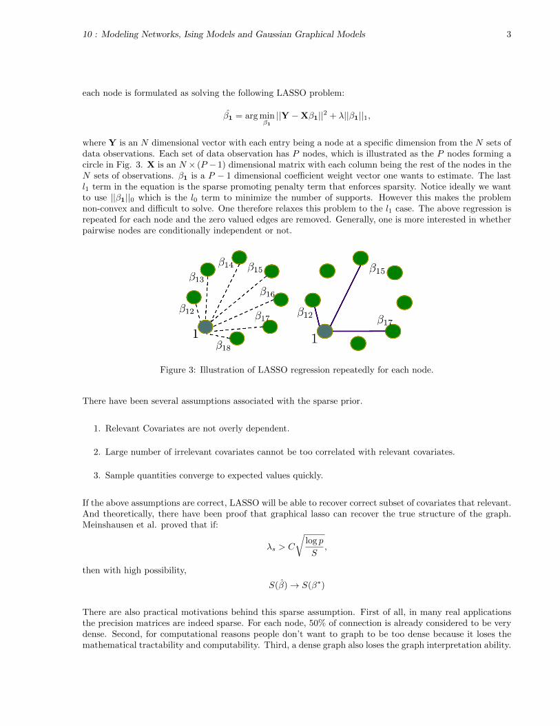
each node is formulated as solving the following LASSO problem:

β̂1 = arg minβ1

||Y −Xβ1||2 + λ||β1||1,

where Y is an N dimensional vector with each entry being a node at a specific dimension from the N sets ofdata observations. Each set of data observation has P nodes, which is illustrated as the P nodes forming acircle in Fig. 3. X is an N × (P − 1) dimensional matrix with each column being the rest of the nodes in theN sets of observations. β1 is a P − 1 dimensional coefficient weight vector one wants to estimate. The lastl1 term in the equation is the sparse promoting penalty term that enforces sparsity. Notice ideally we wantto use ||β1||0 which is the l0 term to minimize the number of supports. However this makes the problemnon-convex and difficult to solve. One therefore relaxes this problem to the l1 case. The above regression isrepeated for each node and the zero valued edges are removed. Generally, one is more interested in whetherpairwise nodes are conditionally independent or not.

Figure 3: Illustration of LASSO regression repeatedly for each node.

There have been several assumptions associated with the sparse prior.

1. Relevant Covariates are not overly dependent.

2. Large number of irrelevant covariates cannot be too correlated with relevant covariates.

3. Sample quantities converge to expected values quickly.

If the above assumptions are correct, LASSO will be able to recover correct subset of covariates that relevant.And theoretically, there have been proof that graphical lasso can recover the true structure of the graph.Meinshausen et al. proved that if:

λs > C

√log p

S,

then with high possibility,

S(β̂)→ S(β∗)

There are also practical motivations behind this sparse assumption. First of all, in many real applicationsthe precision matrices are indeed sparse. For each node, 50% of connection is already considered to be verydense. Second, for computational reasons people don’t want to graph to be too dense because it loses themathematical tractability and computability. Third, a dense graph also loses the graph interpretation ability.


3 Why Does The Basic MB Algorithm Work?

We have presented the algorithm where the inverse covariance matrix is estimated by repeatedly runningLASSO regression on each node. We need to justify why we can do it in this way. For the purpose of thejustification, there are some basic facts that one will use.

3.1 Computing Matrix Inverse

Suppose we have:

M =

[E FG H

],

We can diagonalize the matrix as:[I −FH−10 I

] [E FG H

] [I 0−H−1G I

]=

[E − FH−1G 00 H

].

Also denote M/H = E − FH−1G. Using the formula XY Z = W ⇒ Y −1 = ZW−1X, we have

M−1 =

[E FG H

]−1=

[I 0−H−1G I

] [(M/H)−1 00 H−1

] [I −FH−10 I

]=

[(M/H)−1 −(M/H)−1FH−1

−H−1G(M/H)−1 H−1 +H−1G(M/H)−1FH−1

].

3.2 Relation between Precision Matrix and Covariance Matrix

Suppose we have:

Σ =

[σ11 ~σ>1~σ1 Σ−1

]Also recall the facts about matrix inverse derived in the previous section, we can have:

Q =

[q11 −q11~σ>1 Σ−1−1−q11Σ−1−1~σ

>1 Σ−1−1(I + q11)~σ1~σ

>1 Σ−1−1

]=

[q11 ~q>1~q1 Q−1

]

3.3 Conditional Probabilities in Multivariate Gaussian

Consider the multivariate Gaussian density:

p(x|µ,Σ) =1

(2π)n/2|Σ|1/2exp(−1

2(x− µ)>Σ−1(x− µ)).

We can rewrite the joint Gaussian as:

p(

[x1

x2

]|µ,Σ) = N (

[x1

x2

]|[µ1

µ2

],

[Σ11 Σ12

Σ21 Σ22

])

Using the above notations, we have the following important fact:

p(x1|x2) = N (x1|m1|2,V1|2),

where we have:m1|2 = µ1 + Σ12Σ−122 (x2 − µ2)

V1|2 = Σ11 − Σ12Σ−122 Σ21


3.4 The justification

With the above three facts, one is ready to justify why the problem can be formulated as a LASSO variableselection problem. Given a Gaussian distribution, the conditional distribution of a single node i given therest of the nodes can be written as:

p(Xi|X−i) = N (µi + ΣXiX−iΣ−1XiX−i

(X−i − µX−i),ΣXiXi − ΣXiX−iΣ−1X−iX−i

ΣX−iXi)

Without loss of generality, one has:

p(Xi|X−i) = N (ΣXiX−iΣ−1XiX−i

(X−i),ΣXiXi− ΣXiX−i

Σ−1X−iX−iΣX−iXi

)

= N (~σ>i Σ−1−iX−i, qi|−i)

= N (~q>i−qii

X−i, qi|−i)

From here one can already see that the value of a certain node is determined by the linear representation ofthe other nodes plus a Gaussian noise:

Xi ← βiX−i + Noise(Gaussain).

If the assumption about sparse structure is correct, then the structure can be correctly recovered via LASSO.The estimated graph structure can be written as:

Si ≡ {j : j 6= i, βij 6= 0}.

4 Alternative Methods in Graphical Structure Learning

4.1 The Graphical Lasso Algorithm

There have been more robust and faster algorithms to handle this problem. One of the problem with thebasic MB algorithm is that “The loss function is lost”. Recall that we have the Multivariate Gaussian densityfunction which can be written as:

p(x|µ,Σ) =|Q|1/2

(2π)n/2exp(−1

2(x− µ)>Q(x− µ)).

We want to estimate the precision matrix Q via an l1-regularized maximum likelihood estimation methodsuch that Q is sparse. Therefore the cost function J is the regularized likelihood. Taking the log of thedensity function, one has:

log p(x|µ,Σ) ∝ log detQ− (x− µ)>Q(x− µ)

= log detQ− Tr((x− µ)>Q(x− µ))

= log detQ− Tr((x− µ)(x− µ)>Q)

= log detQ− Tr(SQ)

Therefore putting it together with the l1 regularizer one has:

J(Q) = log detQ− Tr(SQ)− ρ||Q||1Q∗ = arg max

Q(log detQ− Tr(SQ)− ρ||Q||1)


Figure 4: Illustration of updating Q in Graphical LASSO.

Different from MB, the LASSO problems are coupled. Such joint loss function makes the method morestable under noise. The optimization of the above problem is decoupled into updating a row and a columneach time in Q. As is illustrated in Fig. 4. Note that the optimization is taken for the blue vectors in thematrix each time. The optimization problem is shown to be LASSO (l1-regularized quadratic programming).After each optimization, the corresponding row and column are permuted and the new row and column areupdated. This process is repeated untill convergence.

4.2 Learning Ising Model for Pairwise MRF

The problem of learning is to deduce the graphical model of a set of random variables given statistics of the random variables. The Ising model is a famous model in statistical physics that has been used as simple model of magnetic phenomena and of phase transitions in complex systems. It is a certain class of binary-variable graphical models with pairwise interactions. We write the P (x|Θ) to denote likelihood of the Ising model, where θii is the vertex parameter and θij is the edge parameter, and xi is the node of the model. The neighborhood selection for this model is built on the logistic regression, which is the L1-regulaerized logistic regression. The theory flow is as follows: Assumingthe nodes are discrete (e.g., voting outcome of a person), and edges are weighted, then for a sample x, we have

P (x|Θ) = exp(∑i∈V

θtiixi +∑

(i,j)∈E

θijxixj )− A(Θ))

It can be shown the pseudo-conditional likelihood for node k is

P0(xk|x/k) = logistic(2xk < θ/k, x/k >)

5 Dealing with Evolving Networks

So far is the theory, the following section will take this forward into the real word and address some interesting application problems. The social network in the congress is a very interesting problem because the graph exists in this network is estimated from the algorithm, instead of the real data. No congress people will tell us who are their friends and who are their enemies, for these are the top secrets, and furthermore, they are changing over time. So how can we do that? The data is kind of strange, which is from the ballet box. The behavior of the congress people can reflect their political opinion. So they cast vote on different bills. A very interesting problem here is what the social network is at every point and on every bill, which is underlying the voting behavior. We can also turn this question into gene expression or Facebook friendship network, and anything where you see the behavior, instead of the network. This is a very generic problem, even in the Facebook, this is still valid because the Facebook has a graph for you, but those graphs are not the real one. People dont actually interact with all the friends on the friends list. People also do not actually know who you are interacting with. So this is an evolving social network problem because the network is changing over time.


Figure 5: The evolving social network.

The evolving property which increases the additional difficulty in this problem is that you are down to an extreme case of the sample sparsity. You will have an inference problem of p dimensional network from one sample. p will be much larger than 1. This gives rise to a new problem of non-parametric inference of graphical model.

The first inference algorithm is KELLER: Kernel Weighted L1-regularized Logistic Regression. This algo-rithm still does the neighborhood selection for the network. But a little bit re-engineering of the loss function.The loss function is as follows:

lω(θti) =

T∑t′=1

ω(xt′;xt)logP (xt

′

i , θti)

As defined in section 4.2, θi is the vertex parameter and xi is the node of the model. This loss function is just the sum of the regression loss, which is the conditional likelihood of one node given another node. If we only have one sample, we can sum over time. But we have another problem that the network at the next time (t+1) is different from the network at time t. In order to estimate the network at time t, we introduce the kernel function with the assumption that the network has a smooth change. we are going to re-weight every time specific regression conditional likelihood, with the kernel that measure the difference of that point to the time point that estimating the network. This is called the kernel reweighting technique. We can get a virtual data, for which we still sample over time, but the sample at other time will get down weighted. We can thus re-write the neighborhood selection function, which in this case is the logistic regression function with the discrete nodes.

The L-1 norm regression problem is as follows:

where,

γ(θti ;xt) = logPθti (x

ti|xt/i)

ωt(t∗) =

Khn(t− t∗)∑t′∈Tn Khn

(t′ − t∗)

Pθt(xi

t|xt\i) = logistic(2xi

t< θt\i, xt

\i >)


The only difference is that we have the re-weighting function over the original regression loss. We can usethe Gaussian kernel to define the weight, as illustrated as the following graph:

Figure 6: Gaussian kernel to define the weight.

The statistical property of this method are: Dependency Condition; Incoherence Condition; SmoothnessCondition and Bounded Kernel.

The second inference algorithm is TESLA: Temporally Smoothed L1-regularized logistic regression. TESLAhas the similar idea with KELLER, but using slightly different technique in controlling the coupling betweenmultiple graphs. The problem formulation is as follows:

where,

There are two steps for the estimation procedure: 1) estimate block partition on which the coefficientfunctions are constant, and 2) estimate the coefficient functions on each block of the partition.

For the last part of the lecture, Professor gave us two stories regarding the finding of such technique: 1)Senate network, and 2) Progression and Reversion of Breast Cancer cells. To justify the graphical estimationis very difficult. We prefer to run on some data set where we at least know if we can justify the efficacy ornot. For instance, we all know that there are two major parties in American politics. If the algorithm failsto reflect that, it does not make sense.

6 Summary

This Lecture has three major parts: Gaussian Graphical Model; Neighborhood selection and Time-varying Markov networks. We have learnt Gaussian Graphical Model to capture graph topology in multivariable domain; we have learnt the neighborhood selection to perform that kind of estimation, we have also learnt the KELLER and TESLA methods to do the time variant network estimation.

10 : Modeling Networks, Ising Models and Gaussian...

Documents

Transcript of 10 : Modeling Networks, Ising Models and Gaussian...