10 DECISIONS SPRODUCTION - · PDF filethe concept of the product life cycle. Most products...

10 THE FIRM’S PRODUCTIONDECISIONS

LEARNING OBJECTIVES

In this chapter you will:

• Revisit the meaning of competition and a competitivemarket

• Look at the conditions under which a competitive firmwill shut down temporarily

• Examine the conditions under which a firm will chooseto exit a market

• See why sunk costs can be ignored in productiondecisions

• Cover the difference between normal and abnormalprofit and howmaking normal or zero profit still means itis worth continuing in production

• See how the supply curve for a competitive firm isderived in the short run and the long run

• Cover the difference in the equilibrium position of acompetitive firm in the short run and the long run

After reading this chapter you should be able to:

• State the assumptions of the model of a highlycompetitive firm

• Calculate and draw cost and revenue curves and showthe profit-maximizing output

• Show, using diagrams and basic maths, the conditionsunder which a firm will shut down temporarily and exitthe market in the long run

• Explain the difference between normal and abnormalprofit

• Explain why a firm will continue in production even if itmakes zero profit

• Use diagrams to explain the short- and long-runequilibrium position for a firm in a highly competitivemarket

237

INTRODUCTION

In Chapters 8 and 9 we looked at a firm’s costs and revenues and the various goals of abusiness. In this chapter we are going to look at the implications of these for decisionsabout how much to supply and about when to cease production. Chapter 8 introducedthe concept of the product life cycle. Most products will have a product life cycle whichincludes the phases from launch, through growth maturity and decline. Firms will have tomake decisions about levels of production during these phases and when a product reachesthe decline stage a decision will need to be made about whether to continue production.

Firms are affected by the general state of the economy and changing tastes and fash-ions. In times of economic downturn, some firms will find that demand for their productfalls to such an extent that it becomes impossible to continue production and so closedown. VHS video recorders and cathode ray tube TVs are no longer produced by mostof the major electrical manufacturers for example. Such external effects mean that deci-sions will have to be taken on changes to production levels and indeed whether produc-tion should continue at all. We will look at the principles governing these decisions inthis chapter.

Competitive Markets – A Refresher

In Chapter 4 we looked at the nature of competitive markets. As background to thematerial we are going to cover in this chapter, let us remind ourselves of the main prin-ciples. If an individual petrol station raised the price it charges for petrol by 20 per centit would be likely to see a large drop in the amount of petrol it sold. Its customers wouldquickly switch to buying their petrol at other petrol stations. By contrast, if your regionalwater company raised the price of water by 20 per cent, it would see only a smalldecrease in the amount of water it sold. People might look to use water in more efficientways but they would be hard pressed to reduce water consumption greatly and would beunlikely to find another supplier. The difference between the petrol market and the watermarket is obvious: there are many firms selling petrol in many areas but there is onlyone firm selling water. As you might expect, this difference in market structure shapesthe pricing and production decisions of the firms that operate in these markets.

Recall that a market is competitive if each buyer and seller is small compared to thesize of the market and, therefore, has little ability to influence market prices. By contrast,if a firm can influence the market price of the good it sells, it is said to have marketpower. We will examine the behaviour of firms with market power in a later chapter.

Our analysis of competitive firms in this chapter will shed light on the decisions thatlie behind the supply curve in a competitive market. Not surprisingly, we will find that amarket supply curve is tightly linked to firms’ costs of production. Among a firm’s vari-ous costs – fixed, variable, average and marginal – which ones are most relevant for itsdecision about the quantity to supply at any given price? We will see that all these mea-sures of cost play important and interrelated roles.

The following represents some basic principles underlying competition and competi-tive markets:

• Where more than one firm offers the same or a similar product there is competition –the more firms there are in the market the more competition there is but the size ofeach firm relative to the total market is important in our analysis.

• Where firms are small in relation to the total market their influence on price is lim-ited and they take on more characteristics of being price takers.

• Competition will manifest itself where substitutes exist: for example, gas and electric-ity are separate markets but there is the opportunity for consumers to substitute gascookers for electric ones and so some element of competition exists.

• The closer the degree of substitutability the greater will be the competition that exists.

238 Part 4 Microeconomics – The Economics of Firms in Markets

• Firms may influence the level of competition through the way they build relationshipswith consumers, encourage purchasing habits, provide levels of customer service andafter sales service, and so on.

Markets will have different degrees of competition. For a market to be at the highlycompetitive end of the scale, a number of characteristics have to exist:

• There are many buyers and many sellers in the market.• The goods offered by the various sellers are largely the same (if identical the goods are

described as being ‘homogenous’).• Firms can freely enter or exit the market.• There is a high degree of information available to buyers and sellers in the market.

An example is the market for milk. No single buyer of milk can influence the price ofmilk because each buyer purchases a small amount relative to the size of the market.Similarly, each seller of milk has limited control over the price because many other sell-ers are offering milk that is essentially identical. It is assumed that because each seller issmall they can sell all they want at the going price. There is little reason to charge less,and if a higher price is charged, buyers will go elsewhere. Buyers and sellers in competi-tive markets must accept the price the market determines and, therefore, are said to beprice takers.

Entry into the dairy industry is relatively easy – anyone can decide to start a dairyfarm and for existing dairy farmers it is relatively easy to leave the industry. It shouldbe noted that much of the analysis of competitive firms does not rely on the assumptionof free entry and exit because this condition is not necessary for firms to be price takers.But as we will see later in this chapter, entry and exit are often powerful forces shapingthe long-run outcome in competitive markets.

The developments in technology now mean that many more people have access toinformation about firms. Price comparison websites, blogs, review sites and so onmean that it is much easier for consumers to find out about the prices being chargedby different firms in a market, as well as the sort of service and quality they offer.Firms can also make use of this information and are aware that they are subject toincreasing transparency over the way they conduct their business. This can affect theirbehaviour.

Having stated these assumptions we can look at how firms behave in such markets.Remember this is a model which allows us to be able to analyze behaviour under theseassumptions. We can then begin to drop some of these assumptions and analyze howfirm behaviour may differ as a result.

The Marginal Cost Curve and the Firm’s Supply Decision

In Chapter 8 we identified the point of profit maximization as the output level wheremarginal cost ¼ marginal revenue (MC ¼ MR). Consider the profit-maximizing positionfor a competitive firm as shown in Figure 10.1. The figure shows a horizontal line at themarket price (P). The price line for a highly competitive firm is horizontal because thefirm is a price taker: the price of the firm’s output is the same, regardless of the quantitythat the firm decides to produce. Remember we are assuming the firm is operating in ahighly competitive market. For a competitive firm, the firm’s price equals both its aver-age revenue (AR) and its marginal revenue (MR). This is because the firm is so smallrelative to the market that it cannot influence price. We also assumed the firm can sellall it wants at the reigning market price. If the firm is currently selling 100 units and themarket price is €2 per unit then the average revenue (AR ¼ TR/Q) will be 200/100 ¼ €2.If it now sells an additional unit at €2 its average revenue will be 202/101 ¼ €2 and themarginal revenue (the addition to total revenue as a result of selling one extra unit) willalso be €2. Therefore under these highly competitive conditions, P ¼ AR ¼ MR.

The dairy industry is not just abouthaving cows and a field – there isplenty of capital investment neededas well to maximize yields.

BASKETMAN23/SHUTTERSTOCK

Chapter 10 The Firm’s Production Decisions 239

Figure 10.2 shows how a competitive firm responds to an increase in the pricewhich may have been caused by a change in global market conditions. Rememberthat competitive firms are price takers and have to accept the market price for theirproduct. Prices of commodities such as grain, metals, sugar, cotton, coffee, pork bellies,oil and so on are set by organized international markets and so the individual firm hasno power to influence price. When the price is P1, the firm produces quantity Q1, the

FIGURE 10.1

Profit Maximization for a Competitive Firm

This figure shows the marginal cost curve (MC), the average total cost curve (ATC) and the average variable cost curve (AVC). It alsoshows the market price (P), which equals marginal revenue (MR) and average revenue (AR). At the quantity Q1, marginal revenue MR1exceeds marginal cost MC1, so raising production increases profit. At the quantity Q2 marginal cost MC2 is above marginal revenue MR2,so reducing production increases profit. The profit-maximizing quantity QMAX is found where the horizontal price line intersects themarginal cost curve.

0 Quantity

Costs

and

revenue

MC2

MC1

P 5 MR1 5 MR2

Q1 Q2QMAX

AVCP 5 AR 5 MR

ATC

MC

The firm maximizes

profit by producing

the quantity at which

marginal cost equals

marginal revenue.

FIGURE 10.2

Marginal Cost as the Competitive Firm’s Supply Curve (1)

An increase in the price from P1 to P2 leads to an increase in the firm’s profit-maximizing quantity from Q1 to Q2. Because the marginalcost curve shows the quantity supplied by the firm at any given price, it is the firm’s supply curve.

0 Quantity

Price

P2

P1

Q1 Q2

MC

AVC

ATC


quantity that equates marginal cost to the price (which remember is the same as mar-ginal revenue). Assume that an outbreak of tuberculosis results in the need to slaughtera large proportion of dairy cattle and as a result there is a shortage of milk on the mar-ket. When the price rises to P2, the individual firm finds that marginal revenue is nowhigher than marginal cost at the previous level of output, so the firm will seek toincrease production (assuming it is not one of the firms whose dairy herd has beenwiped out). The new profit-maximizing quantity is Q2, at which marginal cost equalsthe new higher price. In essence, because the firm’s marginal cost curve determines thequantity of the good the firm is willing to supply at any price, it is the competitivefirm’s supply curve.

A similar, but reversed, situation would occur if the price fell for some reason asshown in Figure 10.3. In this situation, the firm would find that at the initial equilibriumoutput level, Q1, marginal cost would be greater than marginal revenue with a new priceof P2 and so the firm would look to cut back production to the new profit-maximizingoutput level Q2.

The Firm’s Short-Run Decision to Shut Down

Clearly, in reality, the profit-maximizing output might be hard to identify because itrelies on the firm being able to identify all its costs and revenues accurately over a periodof time and to have the capacity to expand and contract quickly in response to changingmarket conditions.

We also know that firms make losses – sometimes very big losses. If we assume that afirm exists to make a profit do we conclude that if it makes a loss it will shut down itsoperations? This is obviously not the case in some situations although at some point a deci-sion to cease operating will be taken. How does the firm make that sort of decision?

We can distinguish between a temporary shutdown of a firm and the permanent exitof a firm from the market. A shutdown refers to a short-run decision not to produceanything during a specific period of time because of current market conditions. Thiswas the case with some firms in the automotive industry during the aftermath of thefinancial crisis in 2008–2010. A number of firms decided to suspend production forvarying periods of time while the market recovered and stocks were reduced.

FIGURE 10.3

Marginal Cost as the Competitive Firm’s Supply Curve (2)

A fall in the price from P1 to P2 leads to a decrease in the firm’s profit-maximizing quantity from Q1 to Q2. The marginal cost curve showsthe quantity supplied by the firm at any given price.

0 Quantity

Price

P1

P2

Q2 Q1

MC

ATC


This is different to a complete cessation of operations referred to as exit. Exit is along-run decision to leave the market. The short-run and long-run decisions differbecause most firms cannot avoid their fixed costs in the short run but can do so in thelong run. A firm that shuts down temporarily still has to pay its fixed costs, whereas afirm that exits the market saves both its fixed and its variable costs.

For example, consider the production decision that an oil producer faces. The cost ofthe land, and the capital equipment to drill and process oil, form part of the producer’sfixed costs. If the firm decides to suspend the supply of oil for two months, the cost ofthe land and capital cannot be recovered. When making the short-run decision whetherto shut down production for a period, the fixed cost of land and capital is said to be asunk cost. By contrast, if the oil producer decides to leave the industry altogether, it cansell the land and some of the capital equipment. When making the long-run decisionwhether to exit the market, the cost of land and capital is not sunk. (We return to theissue of sunk costs shortly.)

Now let’s consider what determines a firm’s shutdown decision in the short run. Ifthe firm shuts down, it loses all revenue from the sale of the products it is not now pro-ducing and which could be sold. At the same time, it does not have to pay the variablecosts of making its product (but must still pay the fixed costs). Common sense would tellus that a firm shuts down if the revenue that it would get from producing is less than itsvariable costs of production; it is simply not worth producing a product which costsmore to produce than the revenue generated by its sale. Doing so would reduce profitor make any existing losses even greater.

A little bit of mathematics can make this shutdown criterion more useful. If TRstands for total revenue and VC stands for variable costs, then the firm’s decision canbe written as:

Shut down if TR < VC

The firm shuts down if total revenue is less than variable cost. By dividing both sidesof this inequality by the quantity Q, we can write it as:

Shut down if TR/Q < VC/Q

Notice that this can be further simplified. TR/Q is total revenue divided by quantity,which is average revenue (AR). For a competitive firm average revenue is simply thegood’s price P. Similarly, VC/Q is average variable cost AVC. Therefore, the firm’s shut-down criterion is:

Shut down if P < AVC

That is, a firm chooses to shut down if the price of the good is less than the averagevariable cost of production. This is our common sense interpretation: when choosing toproduce, the firm compares the price it receives for the typical unit to the average vari-able cost that it must incur to produce the typical unit. If the price doesn’t cover theaverage variable cost, the firm is better off stopping production altogether. The firm canreopen in the future if conditions change so that price exceeds average variable cost.

? what if…the price the firm received was equal to AVC in the long run – wouldthe firm still be able to continue in production indefinitely?

We now have a full description of a competitive firm’s profit-maximizing strategy. If thefirm produces anything, it produces the quantity at which marginal cost equals the priceof the good. Yet if the price is less than average variable cost at that quantity, the firm isbetter off shutting down and not producing anything. These results are illustrated inFigure 10.4. The competitive firm’s short-run supply curve is the portion of its marginalcost curve that lies above average variable cost.

The decision to shut down a firmaffects large numbers of people,not just employees who may losetheir jobs, and can be a lengthyprocess and a costly decision tomake.

©ANDREW

ASHW

IN


Sunk Costs Economists say that a cost is a sunk cost when it has already beencommitted and cannot be recovered. In a sense, a sunk cost is the opposite of an oppor-tunity cost: an opportunity cost is what you have to give up if you choose to do onething instead of another, whereas a sunk cost cannot be avoided, regardless of thechoices you make. Because nothing can be done about sunk costs, you can ignore themwhen making decisions about various aspects of life, including business strategy.

Our analysis of the firm’s shutdown decision is one example of the importanceof recognizing sunk costs. We assume that the firm cannot recover its fixed costs by tem-porarily stopping production. As a result, the firm’s fixed costs are sunk in the short run,and the firm can safely ignore these costs when deciding how much to produce. Thefirm’s short-run supply curve is the part of the marginal cost curve that lies above aver-age variable cost, and the size of the fixed cost does not matter for this supply decision.

The Firm’s Long-Run Decision to Exit or Enter a Market

The firm’s long-run decision to exit the market is similar to its short-run decision insome respects. If the firm exits, it again will lose all revenue from the sale of its product,but now it saves on both fixed and variable costs of production. Thus, the firm exits themarket if the revenue it would get from producing is less than its total costs.

We can again make this criterion more useful by writing it mathematically. If TR standsfor total revenue and TC stands for total cost, then the firm’s criterion can be written as:

Exit if TR < TC

The firm exits if total revenue is less than total cost in the long run. By dividing bothsides of this inequality by quantity Q, we can write it as:

Exit if TR/Q < TC/Q

We can simplify this further by noting that TR/Q is average revenue, which, of coursefor a competitive firm is the same as the price P, and that TC/Q is average total costATC. Therefore, the firm’s exit criterion is:

Exit if P < ATC

That is, a firm chooses to exit if the price of the good is less than the average totalcost of production.

FIGURE 10.4

The Competitive Firm’s Short-Run Supply Curve

In the short run, the competitive firm’s supply curve is its marginal cost curve (MC) above average variable cost (AVC). If the price fallsbelow average variable cost, the firm is better off shutting down.

0 Quantity

Costs

MC

ATC

AVC

Firm’s short-run

supply curve

Firm

shuts

down if

P , AVC

sunk cost a cost that has alreadybeen committed and cannot berecovered


One of the financial objectives for new firms starting up is to make profit. The entrycriterion where some profit will be made is:

Enter if P > ATC

The criterion for entry is exactly the opposite of the criterion for exit.We can now describe a competitive firm’s long-run profit-maximizing strategy. If the

firm is in the market, it aims to produce at the quantity at which marginal cost equalsthe price of the good. Yet if the price is less than average total cost at that quantity, thefirm chooses to exit (or not enter) the market. These results are illustrated in Figure 10.5.The competitive firm’s long-run supply curve is the portion of its marginal cost curvethat lies above average total cost.

C A S E S T U D YProduction Shutdowns

Potash Corp, based in Saskatchewan,Canada, produces fertilizers for agri-culture. It supplies around 20 percent of the world’s supply of potash,a key element in crop nutrients.Given its size, Potash Corp cannotbe described as a highly competitivefirm but it still faces many of theissues that firms in our model face.

Demand for the firm’s products isdependent on the state of the agricul-ture industry. The more acres of landthat are farmed the higher the de-mand for fertilizers like potash and sothe more incentive there is for PotashCorp to supply the market. However,if demand for its products falls then

FIGURE 10.5

The Competitive Firm’s Long-Run Supply Curve

In the long run, the competitive firm’s supply curve is its marginal cost curve (MC) above average total cost (ATC). If the price falls belowaverage total cost, the firm is better off exiting the market.

0 Quantity

Costs

MC

ATC

Firm’s long-run

supply curve

Firm exits

if P , ATC

By shutting down temporarily, Potash Corpwill not have to pay the variable costs ofoperating machinery and mining potashgiven that sluggish demand for potashmeans prices may be lower than thevariable costs of production.

GETTY

IMAGES


the company has to make decisions about production levels. In February 2012, thecompany announced a decision to temporarily shutdown production at one of itsplants in Saskatchewan for four weeks. This decision followed temporary shutdownsin two other plants in Canada, one for 6 weeks which started in late December 2011and the other from January 2012 for 8 weeks.

The reason for the announcements was that demand for potash had slowed,partly due to the global economic position. Buyers were not replenishing stocks ata rate which made it viable to continue production and so the company moved toreduce supply until demand began to pick up. Potash Corp executives suggestedthat demand was expected to pick up in the northern hemisphere spring due torelatively high prices of crops and decisions by farmers to plant more acres as aresult to take advantage of the higher crop prices.

Annual production at the firm’s Allan mine would be reduced by between150 000 to 160 000 metric tonnes; according to reports, around 1.6 per cent of thefirm’s total annual production of potash. Potash Corp noted that workers at theplants would not be laid off, however, but instead would be deployed to otherwork within the company during the shutdown period.

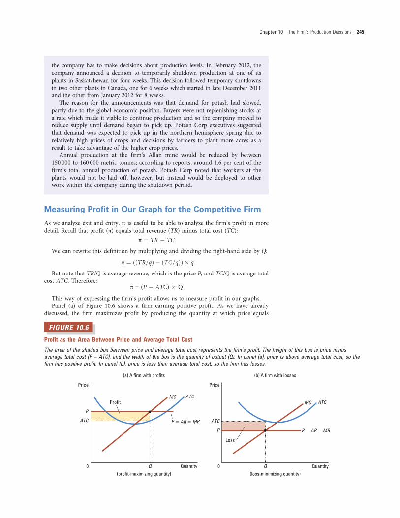
Measuring Profit in Our Graph for the Competitive Firm

As we analyze exit and entry, it is useful to be able to analyze the firm’s profit in moredetail. Recall that profit (π) equals total revenue (TR) minus total cost (TC):

π ¼ TR � TC

We can rewrite this definition by multiplying and dividing the right-hand side by Q:

π ¼ ððTR=qÞ � ðTC=qÞÞ � q

But note that TR/Q is average revenue, which is the price P, and TC/Q is average totalcost ATC. Therefore:

π = (P � ATC) � Q

This way of expressing the firm’s profit allows us to measure profit in our graphs.Panel (a) of Figure 10.6 shows a firm earning positive profit. As we have already

discussed, the firm maximizes profit by producing the quantity at which price equals

FIGURE 10.6

Profit as the Area Between Price and Average Total Cost

The area of the shaded box between price and average total cost represents the firm’s profit. The height of this box is price minusaverage total cost (P − ATC), and the width of the box is the quantity of output (Q). In panel (a), price is above average total cost, so thefirm has positive profit. In panel (b), price is less than average total cost, so the firm has losses.

Price

Quantity0 Q

(a) A firm with profits

(profit-maximizing quantity) (loss-minimizing quantity)

Profit

P 5 AR 5 MR

ATCMC

P

ATC

Price

Quantity0 Q

(b) A firm with losses

P

ATC

Loss

P 5 AR 5 MR

MC ATC


marginal cost. Now look at the shaded rectangle. The height of the rectangle is P � ATC,the difference between price and average total cost. The width of the rectangle is Q, thequantity produced. Therefore, the area of the rectangle is (P � ATC) � Q, which is thefirm’s profit.

Similarly, panel (b) of this figure shows a firm with losses (negative profit). In this case,maximizing profit means minimizing losses, a task accomplished once again by producingthe quantity at which price equals marginal cost. Now consider the shaded rectangle. Theheight of the rectangle is ATC � P, and the width is Q. The area is (ATC � P) � Q, whichis the firm’s loss. Because a firm in this situation is not making enough revenue to cover itsaverage total cost, the firm would choose to exit the market.

Quick Quiz How does the price faced by a profit-maximizing competitive

firm compare to its marginal cost? Explain. • When does a profit-

maximizing competitive firm decide to shut down? When does a profit-

maximizing competitive firm decide to exit a market?

THE SUPPLY CURVE IN A COMPETITIVEMARKET

Now that we have examined the supply decision of a single firm, we can discuss the supplycurve for a market. There are two cases to consider. First, we examine a market with afixed number of firms. Secondly, we examine a market in which the number of firms canchange as old firms exit the market and new firms enter. Both cases are important, for eachapplies over a specific time horizon. Over short periods of time it is often difficult for firmsto enter and exit, so the assumption of a fixed number of firms is appropriate. But overlong periods of time, the number of firms can adjust to changing market conditions.

The Short Run: Market Supply with a Fixed

Number of Firms

Consider first a market with 1000 identical firms. For any given price, each firm suppliesa quantity of output so that its marginal cost equals the price, as shown in panel (a) ofFigure 10.7. That is, as long as price is above average variable cost, each firm’s marginalcost curve is its supply curve. The quantity of output supplied to the market equals thesum of the quantities supplied by each of the 1000 individual firms. Thus, to derive themarket supply curve, we add the quantity supplied by each firm in the market. As panel(b) of Figure 10.7 shows, because the firms are identical, the quantity supplied to themarket is 1000 times the quantity supplied by each firm.

The Long Run: Market Supply with Entry and Exit

Now consider what happens if firms are able to enter or exit the market. Let’s supposethat everyone has access to the same technology for producing the good and access tothe same markets to buy the inputs into production. Therefore, all firms and all potentialfirms have the same cost curves.

Decisions about entry and exit in a market of this type depend on the incentives fac-ing the owners of existing firms and the entrepreneurs who could start new firms. Iffirms already in the market are profitable, then new firms will have an incentive toenter the market. This entry will expand the number of firms, increase the quantity ofthe good supplied, and drive down prices and profits. Conversely, if firms in the marketare making losses, then some existing firms will exit the market. Their exit will reduce


the number of firms, decrease the quantity of the good supplied, and drive up prices andprofits. At the end of this process of entry and exit, firms that remain in the market mustbe making zero economic profit.

Pitfall Prevention When talking about zero economic profit, it is important toremember the distinction between economic profit and accounting profit introduced inChapter 9. When an economist talks of zero profit they are referring to economic profit.

Recall that we can write a firm’s profits as:

Profit ¼ (P � ATC) � Q

This equation shows that an operating firm has zero profit if and only if the price ofthe good equals the average total cost of producing that good. If price is above averagetotal cost, profit is positive, which encourages new firms to enter. If price is less thanaverage total cost, profit is negative, which encourages some firms to exit. The processof entry and exit ends only when price and average total cost are driven to equality.

This analysis has a surprising implication. We noted earlier in the chapter that competi-tive firms produce so that price equals marginal cost. We just noted that free entry and exitforces price to equal average total cost. But if price is to equal both marginal cost and aver-age total cost, these two measures of cost must equal each other. Marginal cost and averagetotal cost are equal, however, only when the firm is operating at the minimum of averagetotal cost. Recall from Chapter 9 that the level of production with lowest average total costis called the firm’s efficient scale. Therefore, the long-run equilibrium of a competitive mar-ket with free entry and exit must have firms operating at their efficient scale.

Panel (a) of Figure 10.8 shows a firm in such a long-run equilibrium. In this figure,price P equals marginal cost MC, so the firm is profit-maximizing. Price also equals aver-age total cost ATC, so profits are zero. New firms have no incentive to enter the market,and existing firms have no incentive to leave the market.

From this analysis of firm behaviour, we can determine the long-run supply curve forthe market. In a market with free entry and exit, there is only one price consistent withzero profit – the minimum of average total cost. As a result, the long-run market supplycurve must be horizontal at this price, as in panel (b) of Figure 10.8. Any price above

FIGURE 10.7

Market Supply with a Fixed Number of Firms

When the number of firms in the market is fixed, the market supply curve, shown in panel (b), reflects the individual firms’ marginal costcurves, shown in panel (a). Here, in a market of 1000 firms, the quantity of output supplied to the market is 1000 times the quantity suppliedby each firm.

Price

0 100 200

(a) Individual firm supply

€2.00

1.00

Quantity (firm)

MC

Price

0 100 000 200 000

(b) Market supply

€2.00

1.00

Quantity (market)

Supply


this level would generate profit, leading to entry and an increase in the total quantitysupplied. Any price below this level would generate losses, leading to exit and a decreasein the total quantity supplied. Eventually, the number of firms in the market adjusts sothat price equals the minimum of average total cost, and there are enough firms to sat-isfy all the demand at this price.

Why Do Competitive Firms Stay in Business If They Make

Zero Profit?

At first, it might seem odd that competitive firms earn zero profit in the long run. Afterall, people start businesses to make a profit. If entry eventually drives profit to zero, theremight seem to be little reason to stay in business.

To understand the zero-profit condition more fully, recall that profit equals total revenueminus total cost, and that total cost includes all the opportunity costs of the firm. In partic-ular, total cost includes the opportunity cost of the time and money that the firm ownersdevote to the business. In the zero-profit equilibrium, the firm’s revenue must compensatethe owners for the time and money that they expend to keep their business going.

Consider an example. Suppose that a farmer had to invest €1 million to open his farm,which otherwise he could have deposited in a bank to earn €50 000 a year in interest. Inaddition, he had to give up another job that would have paid him €30 000 a year. Thenthe farmer’s opportunity cost of farming includes both the interest he could have earnedand the forgone wages – a total of €80 000. This sum must be calculated as part of thefarmer’s total costs. In some situations zero profit is referred to as normal profit – the min-imum amount required to keep factor inputs in their current use. Even if his profit is drivento zero, his revenue from farming compensates him for these opportunity costs.

Keep in mind that accountants and economists measure costs differently. As we dis-cussed in Chapter 9, accountants keep track of explicit costs but usually miss implicitcosts. That is, they measure costs that require an outflow of money from the firm, butthey fail to include opportunity costs of production that do not involve an outflow ofmoney. As a result, in the zero-profit equilibrium, economic profit is zero, but account-ing profit is positive. Our farmer’s accountant, for instance, would conclude that thefarmer earned an accounting profit of €80 000, which is enough to keep the farmer in

FIGURE 10.8

Market Supply with Entry and Exit

Firms will enter or exit the market until profit is driven to zero. Thus, in the long run, price equals the minimum of average total cost, asshown in panel (a). The number of firms adjusts to ensure that all demand is satisfied at this price. The long-run market supply curve ishorizontal at this price, as shown in panel (b).

Price

0

(a) Firm’s zero-profit condition

P 5 minimum

ATC

Quantity (firm)

Price

0

(b) Market supply

Quantity (market)

MC

ATC

Supply

normal profit the minimum amountrequired to keep factors of production intheir current use


business. In the short run as we shall see, profit can be above zero or normal profitwhich is referred to as abnormal profit.

? what if…a firm earned profit which was only 1 per cent less than zero profit.Would it still be worthwhile continuing in production?

A Shift in Demand in the Short Run and Long Run

Because firms can enter and exit a market in the long run but not in the short run, theresponse of a market to a change in demand depends on the time horizon. To see this,let’s trace the effects of a shift in demand. This analysis will show how a market respondsover time, and it will show how entry and exit drive a market to its long-run equilibrium.

Suppose the market for milk begins in long-run equilibrium. Firms are earning zeroprofit, so price equals the minimum of average total cost. Panel (a) of Figure 10.9 showsthe situation. The long-run equilibrium is point A, the quantity sold in the market is Q1,and the price is P1.

Now suppose scientists discover that milk has miraculous health benefits. As a result,the demand curve for milk shifts outward from D1 to D2, as in panel (b). The short-runequilibrium moves from point A to point B; as a result, the quantity rises from Q1 to Q2

and the price rises from P1 to P2. All of the existing firms respond to the higher price byraising the amount produced. Because each firm’s supply curve reflects its marginal costcurve, how much they each increase production is determined by the marginal costcurve. In the new short-run equilibrium, the price of milk exceeds average total cost, sothe firms are making positive or abnormal profit.

Over time, the profit in this market encourages new firms to enter. Some farmers mayswitch to milk production from other farm products, for example. As the number of firmsgrows, the short-run supply curve shifts to the right from S1 to S2, as in panel (c), and thisshift causes the price of milk to fall. Eventually, the price is driven back down to the mini-mum of average total cost, profits are zero and firms stop entering. Thus, the market reachesa new long-run equilibrium, point C. The price of milk has returned to P1, but the quantityproduced has risen to Q3. Each firm is again producing at its efficient scale, but becausemore firms are in the dairy business, the quantity of milk produced and sold is higher.

JEOPARDY PROBLEMWhen the Channel Tunnel wasbuilt between the United King-dom and France, the cost of pro-duction rose dramatically but notsurprisingly given the technicalchallenges of such an engineeringproject. Once opened it soonbecame clear that the firm whichoperated the tunnel, Eurotunnel,would never break even. Whymight this situation have arisenand why is the tunnel still opera-tional despite being loss making?

The Channel Tunnel – what other use could itpossibly have? Does this affect decisions onwhether to shut or restructure the business?

abnormal profit the profit over andabove normal profit

NAUFRAGO

PLANETÁRIO


FIGURE 10.9

An Increase in Demand in the Short Run and Long Run

The market starts in a long-run equilibrium, shown as point A in panel (a). In this equilibrium, each firm makes zero profit, and the priceequals the minimum average total cost. Panel (b) shows what happens in the short run when demand rises from D1 to D2. The equilibriumgoes from point A to point B, price rises from P1 to P2, and the quantity sold in the market rises from Q1 to Q2. Because price now exceedsaverage total cost, firms make profits, which over time encourage new firms to enter the market. This entry shifts the short-run supplycurve to the right from S1 to S2 as shown in panel (c). In the new long-run equilibrium, point C, price has returned to P1 but the quantitysold has increased to Q3. Profits are again zero, price is back to the minimum of average total cost, but the market has more firms tosatisfy the greater demand.

(a) Initial condition

Price

0

P1

Quantity (firm)

Price

0 Q1

P1

Quantity (market)

MC ATC

Firm

(b) Short-run response

(c) Long-run response

Price

P1

P2

Quantity (firm)

Firm

Market

Short-run supply, S1

Long-run

supply

Demand, D1

A

MC ATCProfit

0

Price

P1

P2

Quantity (market)

Market

0 Q1 Q2

Price

P1

Quantity (firm)

Firm

0

Price

Quantity (market)

Market

0 Q1 Q2 Q3

D2

D1

S1

Long-run

supply

A

B

P1

MC ATC

P1

P2

D2

D1

S1

S2

Long-run

supply

A

B

C

Why the Long-Run Supply Curve Might Slope Upward

So far we have seen that entry and exit can cause the long-run market supply curve to behorizontal. The essence of our analysis is that there are a large number of potentialentrants, each of which faces the same costs. As a result, the long-run market supplycurve is horizontal at the minimum of average total cost. When the demand for the


good increases, the long-run result is an increase in the number of firms and in the totalquantity supplied, without any change in the price.

The reality is that the assumptions we have made in our model do not hold in allcases. There are, as a result, two reasons that the long-run market supply curve mightslope upward. The first is that some resources used in production may be available onlyin limited quantities. For example, consider the market for farm products. Anyone canchoose to buy land and start a farm, but the quantity and quality of land is limited. Asmore people become farmers, the price of farmland is bid up, which raises the costs of allfarmers in the market. Thus, an increase in demand for farm products cannot induce anincrease in quantity supplied without also inducing a rise in farmers’ costs, which in turnmeans a rise in price. The result is a long-run market supply curve that is upward slop-ing, even with free entry into farming.

A second reason for an upward sloping supply curve is that firms may have differ-ent costs. For example, consider the market for painters. Anyone can enter the mar-ket for painting services, but not everyone has the same costs. Costs vary in partbecause some people work faster than others, use different materials and equipmentand because some people have better alternative uses of their time than others. Forany given price, those with lower costs are more likely to enter than those with highercosts. To increase the quantity of painting services supplied, additional entrants mustbe encouraged to enter the market. Because these new entrants have higher costs, theprice must rise to make entry profitable for them. Thus, the market supply curve forpainting services slopes upward even with free entry into the market.

Notice that if firms have different costs, some firms earn profit even in the longrun. In this case, the price in the market reflects the average total cost of the marginalfirm – the firm that would exit the market if the price were any lower. This firm earnszero profit, but firms with lower costs earn positive profit. Entry does not eliminatethis profit because would-be entrants have higher costs than firms already in the mar-ket. Higher-cost firms will enter only if the price rises, making the market profitablefor them.

Thus, for these two reasons, the long-run supply curve in a market may be upwardsloping rather than horizontal, indicating that a higher price is necessary to induce alarger quantity supplied. Nevertheless, the basic lesson about entry and exit remainstrue. Because firms can enter and exit more easily in the long run than in the shortrun, the long-run supply curve is typically more elastic than the short-run supplycurve.

Quick Quiz In the long run with free entry and exit, is the price in a

market equal to marginal cost, average total cost, both, or neither? Explain

with a diagram.

CONCLUSION: BEHIND THE SUPPLY CURVE

We have been discussing the behaviour of competitive profit-maximizing firms. You mayrecall from Chapter 1 that one of the Ten Principles of Economics is that rational peoplethink at the margin. This chapter has applied this idea to the competitive firm. Marginalanalysis has given us a theory of the supply curve in a competitive market and, as aresult, a deeper understanding of market outcomes.

We have learned that when you buy a good from a firm in a competitive market, youcan be assured that the price you pay is close to the cost of producing that good. In par-ticular, if firms are competitive and profit-maximizing, the price of a good equals the


marginal cost of making that good. In addition, if firms can freely enter and exit themarket, the price also equals the lowest possible average total cost of production.

Although we have assumed throughout this chapter that firms are price takers, manyof the tools developed here are also useful for studying firms in less competitive markets.In subsequent chapters we will examine the behaviour of firms with market power. Mar-ginal analysis will again be useful in analyzing these firms, but it will have quite differentimplications.

IN THE NEWS

The Tablet MarketBusinesses like Apple, Samsung and Microsoft are hardly the epitome of the perfectly com-petitive firm that we have been describing, but the market dynamics in which they operate canbear some comforting resemblances to the model outlined in this chapter.

Tablet Growth

There are few people in the world todaywho are not touched in some way bymobile devices. Ever since the mobilephone became a product accessible tovery large numbers of people, firmshave been looking to find ways ofexpanding the mobile technology mar-ket. The development of text messag-ing, emails, the web, listening to music,playing games and watching videohave all been included on mobiledevices with varying degrees of suc-cess over the last ten years.

Apple’s introduction of the iPaddeveloped a new concept in mobiledevices – the tablet. Tablet computersare a mobile device that function verysimilarly to a personal computer andare characterized by a touch screenwhich can be operated by hands orsome sort of pen device.

The iPad was launched in January2010. Since that time sales rose quicklyreaching 1 million by May 2010 andaround 25 million by June 2011. TheiPad 2 was released in March 2011and the iPad 3 a year later. The successof the iPad made it clear that there wasa demand for these types of devicesand that there were potential profitsto be made – Apple reported its fiscal

fourth quarter profits of $6.62 billion inOctober 2011 (not all of this profit isattributed to the iPad of course).Apple was one of the first companiesto launch a tablet PC but other electri-cal manufacturers were not far behindand saw the market potential.

When the iPad was first introduced,the price was relatively high atbetween €500 to €950 depending onthe model. The abnormal profits thatcould be earned on these devicesmeant that there was an incentive forrivals to follow suit and launch theirown tablet PC versions. Amazon hadlaunched its Kindle in 2007 but thisdevice did not have the functionalityof an iPad and was more of an eBookservice than a tablet PC. There hadbeen other tablet PC devices prior tothe iPad but Apple did have the advan-tage of launching at a time when 3Gand wi-fi access was more widelyavailable and accessible.

Following the release of the iPad,the Galaxy Tab from Samsung,Research in Motion’s BlackBerry Play-book, Vizio’s Via, the Toshiba Thrive,LG’s Optimus and the Motorola Xoomall appeared on the market. Amazonsought to get in on the act by updatingits Kindle to the Kindle Fire whichincluded far more functionality, mimick-

ing a tablet PC. A host of other technol-ogy firms also introduced tablets suchas Disgo, Creative, Acer, Archos, HTCand Dell.

How the market reacts to this influxof supply is dependent on the degreeof substitutability between these dif-ferent devices. This is not a perfectmarket with homogenous productsand each device is different in termsof looks, functionality and usability.We are not talking about an industrysupply curve, therefore, that is thesummation of individual firm’s supplycurves.

However, for the consumer, theeffect is that they have a far widerchoice and with greater choice andcompetition between sellers, the pres-sure on prices to fall exists. Along withgreater competition come the improve-ments in production techniques andknowledge, which individual manufac-turers will be looking to exploit to lowerproduction costs and increase produc-tivity and efficiency, thus allowing them

IQONCEPT/SHUTTERSTOCK


to have more flexibility on pricing inwhat is a growing and increasinglycompetitive market.

The result has been a gradualreduction in the prices of tablet PCsas competition and production effi-ciencies rise. The iPad 2, for example,was launched at prices around€50 per model less than the iPad 1.Other devices are being marketed atprices between €50 and €500. Accord-ing to analysts’ reports, the tablet PCmarket is in the early phases of its lifecycle. The predictions for tabletsbased on an optimistic, a most likely

and worst case scenario suggeststhat the growth of the tablet has along way to go yet.

Questions1. Apple was one of the first busi-

nesses to enter the tablet PC mar-ket. What costs would it have hadto take into account in decidingwhether the market was worthentering?

2. Our model assumes freedom ofentry and exit for a market thatmay not be present in marketswhich are not highly competitive.

Outline some factors that might pre-vent entry into the tablet PC market.

3. Using diagrams, explain how short-run profits in the tablet PC industrymight be competed away in the longterm to lead to normal profits beingmade in this market.

4. What factors might affect the lengthof time which could constitute thelong run in the tablet PC market?

5. Assess the factors which wouldallow a firm like Apple to continuemaking abnormal profits in the longrun in this market.

SUMMARY

• Because a competitive firm is a price taker, its revenue isproportional to the amount of output it produces. The priceof the good equals both the firm’s average revenue and itsmarginal revenue.

• To maximize profit, a firm chooses a quantity of output suchthat marginal revenue equals marginal cost. Because mar-ginal revenue for a competitive firm equals the marketprice, the firm chooses quantity so that price equals mar-ginal cost. Thus, the firm’s marginal cost curve is its supplycurve.

• In the short run when a firm cannot recover its fixed costs,the firm will choose to shut down temporarily if the price ofthe good is less than average variable cost. In the long run

when the firm can recover both fixed and variable costs, itwill choose to exit if the price is less than average total cost.

• In a market with free entry and exit, profits are driven to zeroin the long run. In this long-run equilibrium, all firms produceat the efficient scale, price equals the minimum of averagetotal cost, and the number of firms adjusts to satisfy thequantity demanded at this price.

• Changes in demand have different effects over different timehorizons. In the short run, an increase in demand raises pricesand leads to profits, and a decrease in demand lowers pricesand leads to losses. But if firms can freely enter and exit themarket, then in the long run the number of firms adjusts todrive the market back to the zero-profit equilibrium.

KEY CONCEPTS

sunk cost, p. 243 normal profit, p. 248 abnormal profit, p. 249

QUEST IONS FOR REVIEW1. What is meant by a competitive firm?2. Draw the cost curves for a typical firm. For a given price,

explain how the firm chooses the level of output that max-imizes profit.

3. Under what conditions will a firm shut down temporarily?Explain.

4. Under what conditions will a firm exit a market? Explain.

5. Under what conditions will a firm enter a market? Explain.

6. Does a firm’s price equal marginal cost in the short run, inthe long run, or both? Explain.

7. Does a firm’s price equal the minimum of average total costin the short run, in the long run, or both? Explain.

8. Explain why a firm will continue in production even if itmakes zero profit.

9. If a firm is making abnormal profit in the short run, what willhappen to these profits in the long run assuming the con-ditions for a highly competitive market exist?

10. Are market supply curves typically more elastic in the shortrun or in the long run? Explain.


PROBLEMS AND APPL ICAT IONS1. What are the characteristics of a competitive market?

Which of the following drinks do you think is best describedby these characteristics? Why aren’t the others?a. tap waterb. bottled waterc. colad. beer

2. Your flatmate’s long hours in the chemistry lab finally paidoff – she discovered a secret formula that lets people do anhour’s worth of studying in 5 minutes. So far, she’s sold 200doses, and faces the following average total cost schedule:

Q

Average

total cost

199 €199

200 200

201 201

If a new customer offers to pay your flatmate €300 for onedose, should she make one more? Explain.

3. You go out to the best restaurant in town and order a lobsterdinner for €40. After eating half of the lobster, you realizethat you are quite full. Your date wants you to finish yourdinner, because you can’t take it home and because ‘you’vealready paid for it’. What should you do? Relate your answerto the material in this chapter.

4. PC Camera GmBH faces costs of production as follows:

Quantity

Total fixed

costs (€)

Total variable

costs (€)

0 100 0

1 100 50

2 100 70

3 100 90

4 100 140

5 100 200

6 100 360

a. Calculate the company’s average fixed costs, averagevariable costs, average total costs and marginal costs ateach level of production.

b. The price of a PC camera is €50. Seeing that he can’tmake a profit the chief executive officer (CEO) decides toshut down operations. What are the firm’s profits/losses?Was this a wise decision? Explain.

c. Vaguely remembering her introductory business eco-nomics course, the chief financial officer (CFO) tells theCEO it is better to produce 1 PC camera because mar-ginal revenue equals marginal cost at that quantity. Whatare the firm’s profits/losses at that level of production?Was this the best decision? Explain.

5. ‘High prices traditionally cause expansion in an industry,eventually bringing an end to high prices and manufac-turers’ prosperity.’ Explain, using appropriate diagrams.

6. Suppose the book printing industry is competitive andbegins in long-run equilibrium.a. Draw a diagram describing the typical firm in the industry.b. Hi-Tech Printing Company invents a new process that

sharply reduces the cost of printing books. What hap-pens to Hi-Tech’s profits and the price of books in theshort run when Hi-Tech’s patent prevents other firmsfrom using the new technology?

c. What happens in the long run when the patent expiresand other firms are free to use the technology?

7. Many small boats are made of fibreglass, which is derivedfrom crude oil. Suppose that the price of oil rises.a. Using diagrams, show what happens to the cost curves

of an individual boat-making firm and to the market sup-ply curve.

b. What happens to the profits of boat-makers in the shortrun? What happens to the number of boat-makers in thelong run?

8. Suppose that the European Union textile industry is com-petitive, and there is no international trade in textiles. Inlong-run equilibrium, the price per unit of cloth is €30.a. Describe the equilibrium using graphs for the entire

market and for an individual producer.Now suppose that textile producers in non-EU coun-

tries are willing to sell large quantities of cloth in the EUfor only €25 per unit.

b. Assuming that EU textile producers have large fixedcosts, what is the short-run effect of these imports onthe quantity produced by an individual producer? Whatis the short-run effect on profits? Illustrate your answerwith a graph.

c. What is the long-run effect on the number of EU firms inthe industry?

9. Assume that the gold-mining industry is competitive.a. Illustrate a long-run equilibrium using diagrams for the

gold market and for a representative gold mine.b. Suppose that an increase in jewellery demand induces a

surge in the demand for gold. Using your diagrams frompart (a), show what happens in the short run to the goldmarket and to each existing gold mine.

c. If the demand for gold remains high, what would happento the price over time? Specifically, would the new long-run equilibrium price be above, below or equal to theshort-run equilibrium price in part (b)? Is it possible forthe new long-run equilibrium price to be above the origi-nal long-run equilibrium price? Explain.

10. The liquorice industry is competitive. Each firm produces2 million liquorice bootlaces per year. The bootlaces have anaverage total cost of €0.20 each, and they sell for €0.30.a. What is the marginal cost of a liquorice bootlace?b. Is this industry in long-run equilibrium? Why or why not?


10 DECISIONS SPRODUCTION - · PDF filethe concept of the product life cycle. Most products...

Documents

Transcript of 10 DECISIONS SPRODUCTION - · PDF filethe concept of the product life cycle. Most products...