10 CHI-SQUARE TESTS AND THE F-DISTRIBUTION
58
10.1 Goodness-of-Fit Test 10.2 Independence CASE STUDY 10.3 Comparing Two Variances 10.4 Analysis of Variance USES AND ABUSES REAL STATISTICS– REAL DECISIONS TECHNOLOGY Crash tests performed by the Insurance Institute for Highway Safety demonstrate how a vehicle will react when in a realistic collision. Tests are performed on the front, side, and rear of the vehicles. Results of these tests are classified using the ratings good, acceptable, marginal, and poor. 10 CHAPTER CHI-SQUARE TESTS AND THE F -DISTRIBUTION
Transcript of 10 CHI-SQUARE TESTS AND THE F-DISTRIBUTION

10.1 Goodness-of-Fit Test10.2 Independence
! CASE STUDY
10.3 Comparing TwoVariances
10.4 Analysis of Variance! USES AND ABUSES
! REAL STATISTICS–REAL DECISIONS
! TECHNOLOGY
Crash tests performed by the InsuranceInstitute for Highway Safety demonstrate howa vehicle will react when in a realistic collision.Tests are performed on the front, side, and rear of the vehicles. Results of these tests are classified using the ratings good, acceptable,marginal, and poor.
10C H A P T E R
CHI-SQUARETESTS AND THE F-DISTRIBUTION

539
W H E R E Y O U ’ V E B E E N
The Insurance Institute for Highway Safety buysnew vehicles each year and crashes them into a barrier at 40 miles per hour to compare how different vehicles protect drivers in a frontal offset crash. In this test, 40% of the total width ofthe vehicle strikes the barrier on the driver side.The forces and impacts that occur during a crashtest are measured by equipping dummies withspecial instruments and placing them in the car.The crash test results include data on head, chest,and leg injuries. For a low crash test number, theinjury potential is low. If the crash test number ishigh, then the injury potential is high. Using thetechniques of Chapter 8, you can determine ifthe mean chest injury potential is the same forpickups and minivans. (Assume the population
variances are equal.) The sample statistics are asfollows. (Adapted from Insurance Institute for
Highway Safety)
For the means of chest injury, the P-value for thehypothesis that is about 0.7575. At
you fail to reject the null hypothesis.So, you do not have enough evidence to conclude that there is a significant difference inthe means of the chest injury potential in afrontal offset crash at 40 miles per hour for minivans and pickups.
a = 0.05,m1 = m2
""
W H E R E Y O U ’ R E G O I N G
In Chapter 8, you learned how to test a hypothesis that compares two populations bybasing your decisions on sample statistics andtheir distributions. In this chapter, you will learnhow to test a hypothesis that compares three ormore populations.
For instance, in addition to the crash tests forminivans and pickups, a third group of vehicleswas also tested. The results for all three types ofvehicles are as follows.
From these three samples, is there evidence of a difference in chest injury potential amongminivans, pickups, and midsize SUVs in a frontaloffset crash at 40 miles per hour?
In this chapter, you will learn that you cananswer this question by testing the hypothesisthat the three means are equal. For the means ofchest injury, the P-value for the hypothesis that
is about 0.0088. At youcan reject the null hypothesis. So, you can conclude that for the three types of vehicles tested, at least one of the means of the chestinjury potential in a frontal offset crash at 40 miles per hour is different from the others.
a = 0.05,m1 = m2 = m3
""
Vehicle NumberMean
chest injuryStandarddeviation
Minivans n1 = 9 x1 = 29.9 s1 = 3.33Pickups n2 = 19 x2 = 30.4 s2 = 4.21
Vehicle NumberMean
chest injuryStandarddeviation
Minivans n1 = 9 x1 = 29.9 s1 = 3.33Pickups n2 = 19 x2 = 30.4 s2 = 4.21Midsize SUVs n3 = 32 x3 = 34.1 s3 = 5.22

540 C H A P T E R 1 0 CHI-SQUARE TESTS AND THE F -DISTRIBUTION
" THE CHI-SQUARE GOODNESS-OF-FIT TESTSuppose a tax preparation company wants to determine the proportions of people who used different methods to prepare their taxes. To determine theseproportions, the company can perform a multinomial experiment. A multinomialexperiment is a probability experiment consisting of a fixed number of independent trials in which there are more than two possible outcomes for eachtrial.The probability of each outcome is fixed, and each outcome is classified into categories. (Remember from Section 4.2 that a binomial experiment has only twopossible outcomes.)
Now, suppose the company wants to test a previous survey’s claim concerningthe distribution of proportions of people who used different methods to preparetheir taxes. To do so, the company could compare the distribution of proportionsobtained in the multinomial experiment with the previous survey’s specified distribution. How can the company compare the distributions? The answer is,perform a chi-square goodness-of-fit test.
To begin a goodness-of-fit test, you must first state a null and an alternativehypothesis. Generally, the null hypothesis states that the frequency distributionfits the specified distribution and the alternative hypothesis states that thefrequency distribution does not fit the specified distribution.
For instance, suppose the previous survey claims that the distribution of people who used different methods to prepare their taxes is as shown below.
To test the previous survey’s claim, the company can perform a chi-squaregoodness-of-fit test using the following null and alternative hypotheses.
: The distribution of tax preparation methods is 25% by accountant,20% by hand, 35% by computer software, 5% by friend or family, and15% by tax preparation service. (Claim)
: The distribution of tax preparation methods differs from the claimed orexpected distribution.
Ha
H0
Distribution of tax preparation methods
Accountant 25%
By hand 20%
Computer software 35%
Friend/family 5%
Tax preparation service 15%
The Chi-Square Goodness-of-Fit Test
" How to use the chi-square distribution to test whether afrequency distribution fits a claimed distribution
10.1 Goodness-of-Fit Test
WHAT YOU SHOULD LEARN
A chi-square goodness-of-fit test is used to test whether a frequency distribution fits an expected distribution.
D E F I N I T I O N
INSIGHTThe hypothesis tests described in Sections 10.1 and 10.2 can be used for qualitative data.
S E C T I O N 1 0 . 1 GOODNESS-OF-FIT TEST 541
To calculate the test statistic for the chi-square goodness-of-fit test, you canuse observed frequencies and expected frequencies. To calculate the expected frequencies, you must assume the null hypothesis is true.
E X A M P L E 1
!Finding Observed Frequencies and Expected FrequenciesA tax preparation company randomlyselects 300 adults and asks them how theyprepare their taxes. The results are shownat the right. Find the observed frequencyand the expected frequency for each taxpreparation method. (Adapted from NationalRetail Federation)
!SolutionThe observed frequency for each tax preparation method is the number ofadults in the survey naming a particular tax preparation method. The expectedfrequency for each tax preparation method is the product of the number ofadults in the survey and the probability that an adult will name a particular taxpreparation method. The observed frequencies and expected frequencies areshown in the following table.
!Try It Yourself 1Suppose the tax preparation company randomly selects 500 adults. Find theexpected frequency for each tax preparation method.Multiply 500 by the probability that an adult will name each particular taxpreparation method to find the expected frequencies. Answer: Page A45
Survey results 1n ! 3002Accountant 71
By hand 40
Computer software 101
Friend/family 35
Tax preparation service 53
The observed frequency O of a category is the frequency for the categoryobserved in the sample data.
The expected frequency E of a category is the calculated frequency for the category. Expected frequencies are obtained assuming the specified (orhypothesized) distribution. The expected frequency for the ith category is
where n is the number of trials (the sample size) and is the assumed probability of the ith category.
pi
Ei = npi
D E F I N I T I O N
PICTURING THEWORLD
The pie chart shows the distribution of health care visitsto doctor offices, emergencydepartments, and home visits in a recent year. (Source: National Center for Health Statistics)
A researcher randomly selects200 people and asks them howmany visits they make to thedoctor in a year: 1–3, 4–9, 10 or more, or none. What is theexpected frequency for eachresponse?
None 16.4%
1–3 visits47.2%
4–9 visits23.6%
10 or more visits12.8%
INSIGHTThe sum of the expectedfrequencies always equals the sum of the observed frequencies. For instance, in Example 1 the sum of the observed frequencies and the sum of the expected frequencies are both 300.
Tax preparation method % of people
Observed frequency
Expected frequency
Accountant 25% 71 75300(0.25) =By hand 20% 40 60300(0.20) =Computer software 35% 101 105300(0.35) =Friend/family 5% 35 15300(0.05) =Tax preparation service 15% 53 45300(0.15) =

542 C H A P T E R 1 0 CHI-SQUARE TESTS AND THE F -DISTRIBUTION
For the chi-square goodness-of-fit test to be used, the following must be true.
1. The observed frequencies must be obtained using a random sample.2. Each expected frequency must be greater than or equal to 5.
If the expected frequency of a category is less than 5, it may be possible tocombine it with another category to meet the requirements.
When the observed frequencies closely match the expected frequencies, thedifferences between O and E will be small and the chi-square test statistic will be close to 0. As such, the null hypothesis is unlikely to be rejected. However,when there are large discrepancies between the observed frequencies and theexpected frequencies, the differences between O and E will be large, resulting ina large chi-square test statistic. A large chi-square test statistic is evidence forrejecting the null hypothesis. So, the chi-square goodness-of-fit test is always aright-tailed test.
STUDY TIPRemember that a chi-square distribution is positively skewed and its shape is determined by the degrees of freedom. The graph is not symmetric, but it appears to become more symmetric as the degrees of freedom increase, as shown in Section 6.4.
Performing a Chi-Square Goodness-of-Fit TestVerify that the expected frequency is at least 5 for each category.
IN WORDS IN SYMBOLS1. Identify the claim. State the null and State and
alternative hypotheses.2. Specify the level of significance. Identify 3. Determine the degrees of freedom.4. Determine the critical value. Use Table 6 in
Appendix B.5. Determine the rejection region.
6. Find the test statistic and sketch the sampling distribution.
7. Make a decision to reject or fail to If is in the rejection reject the null hypothesis. region, reject Other-
wise, fail to reject 8. Interpret the decision in the context
of the original claim.
H0.H0 .
x2
x2 = g 1O - E22E
d.f. = k - 1a .
Ha .H0
G U I D E L I N E S
If the conditions listed above are satisfied, then the sampling distribution forthe goodness-of-fit test is approximated by a chi-square distribution with
degrees of freedom, where k is the number of categories. The teststatistic for the chi-square goodness-of-fit test is
where O represents the observed frequency of each category and E representsthe expected frequency of each category.
x2 = g 1O - E22E
k - 1
T H E C H I - S Q U A R E G O O D N E S S - O F - F I T T E S T

S E C T I O N 1 0 . 1 GOODNESS-OF-FIT TEST 543
E X A M P L E 2
!Performing a Chi-Square Goodness-of-Fit TestThe tax preparation methods of adults from a previous survey are distributedas shown in the table at the left below. A tax preparation company randomlyselects 300 adults and asks them how they prepare their taxes. The results are shown in the table at the right below. At perform a chi-square goodness-of-fit test to test whether the distributions are different. (Adaptedfrom National Retail Federation)
!SolutionThe observed and expected frequencies are shown in the table at the left.The expected frequencies were calculated in Example 1. Because the observed frequencies were obtained using a random sample and each expected frequency is at least 5, you can use the chi-square goodness-of-fit test to testthe proposed distribution. The null and alternative hypotheses are as follows.
The distribution of tax preparation methods is 25% by accountant,20% by hand, 35% by computer software, 5% by friend or family, and15% by tax preparation service.
The distribution of tax preparation methods differs from the claimedor expected distribution. (Claim)
Because there are 5 categories, the chi-square distribution has degrees of freedom. With and the critical value
is 13.277. With the observed and expected frequencies, the chi-squaretest statistic is
The graph at the left shows the location of the rejection region. Because isin the rejection region, you should reject the null hypothesis.Interpretation There is enough evidence at the 1% level of significance toconclude that the distribution of tax preparation methods differs from theprevious survey’s claimed or expected distribution.
x2
L 35.121.
+135 - 1522
15+153 - 4522
45
=171 - 7522
75+140 - 6022
60+1101 - 10522
105
x2 = g 1O - E22E
x20 =
a = 0.01,d.f. = 45 - 1 = 4k - 1 =
Ha:
H0:
a = 0.01,
Taxpreparation
method
Observed frequency
Expectedfrequency
Accountant 71 75
By hand 40 60
Computersoftware 101 105
Friend/family 35 15
Taxpreparationservice
53 45
Survey results 1n ! 3002Accountant 71
By hand 40
Computer software 101
Friend/family 35
Tax preparation service 53
Distribution of tax preparation methods
Accountant 25%
By hand 20%
Computer software 35%
Friend/family 5%
Tax preparation service 15%
SC
5 10 15 20 25
02χ = 13.277
α = 0.01
Rejectionregion
2χ
Report 45

544 C H A P T E R 1 0 CHI-SQUARE TESTS AND THE F -DISTRIBUTION
AgesPrevious agedistribution
Surveyresults
0–9 16% 76
10–19 20% 84
20–29 8% 30
30–39 14% 60
40–49 15% 54
50–59 12% 40
60–69 10% 42
70+ 5% 14
Color Frequency, f
Brown 80
Yellow 95
Red 88
Blue 83
Orange 76
Green 78
!Try It Yourself 2A sociologist claims that the age distribution for the residents of a certain cityis different than it was 10 years ago. The distribution of ages 10 years ago isshown in the table at the left.You randomly select 400 residents and record theage of each. The survey results are shown in the table. At perform achi-square goodness-of-fit test to test whether the distribution has changed.
a. Verify that the expected frequency is at least 5 for each category.b. Identify the claimed distribution and state and c. Specify the level of significanced. Determine the degrees of freedom.e. Determine the critical value and the rejection region.f. Find the chi-square test statistic. Sketch a graph.g. Decide whether to reject the null hypothesis.h. Interpret the decision in the context of the original claim.
Answer: Page A45
a .Ha .H0
a = 0.05,
The chi-square goodness-of-fit test is often used to determine whether adistribution is uniform. For such tests, the expected frequencies of the categoriesare equal. When testing a uniform distribution, you can find the expected frequency of each category by dividing the sample size by the number of categories. For instance, suppose a company believes that the number of salesmade by its sales force is uniform throughout the five-day work week. If the sample consists of 1000 sales, then the expected value of the sales for each daywill be 1000>5 = 200.
E X A M P L E 3
!Performing a Chi-Square Goodness-of-Fit TestA researcher claims that the number of different-colored candies in bags of dark chocolate M&M’s is uniformly distributed. To test this claim, you randomly select a bag that contains 500 dark chocolate M&M’s. The results are shown in the table at the left. At perform a chi-square goodness-of-fit test to test the claimed or expected distribution. (Adapted fromMars, Incorporated)
!SolutionThe claim is that the distribution is uniform, so the expected frequencies of thecolors are equal.To find each expected frequency, divide the sample size by thenumber of colors. So, for each color, Because each expected frequency is at least 5 and the M&M’s were randomly selected, youcan use the chi-square goodness-of-fit test to test the claimed distribution. Thenull and alternative hypotheses are as follows.
The distribution of the different-colored candies in bags of darkchocolate M&M’s is uniform. (Claim)
The distribution of the different-colored candies in bags of darkchocolate M&M’s is not uniform.
Because there are 6 categories, the chi-square distribution has degrees of freedom. Using and the critical value
is With the observed and expected frequencies, the chi-square teststatistic is shown in the following table.x0
2 = 9.236.a = 0.10,d.f. = 56 - 1 = 5
k - 1 =
Ha:
H0:
E = 500>6 L 83.33.
a = 0.10,
SC Report 46

S E C T I O N 1 0 . 1 GOODNESS-OF-FIT TEST 545
The graph shows the location of the rejection region and the chi-square teststatistic. Because is not in the rejection region, you should fail to reject thenull hypothesis.
Interpretation There is not enough evidence at the 10% level of significanceto reject the claim that the distribution of the different-colored candies in bagsof dark chocolate M&M’s is uniform.
!Try It Yourself 3A researcher claims that the number of different-colored candies in bags ofpeanut M&M’s is uniformly distributed.To test this claim, you randomly selecta bag that contains 180 peanut M&M’s. The results are shown in the table atthe left. Using perform a chi-square goodness-of-fit test to test theclaimed or expected distribution. (Adapted from Mars, Incorporated)
a. Verify that the expected frequency is at least 5 for each category.b. Identify the claimed distribution and state and c. Specify the level of significanced. Determine the degrees of freedom.e. Determine the critical value and the rejection region.f. Find the chi-square test statistic. Sketch a graph.g. Decide whether to reject the null hypothesis.h. Interpret the decision in the context of the original claim.
Answer: Page A46
a.Ha.H0
a = 0.05,
5 15 20 25
02χ = 9.236 2χ
2χ
≈ 3.016
α = 0.10
Rejectionregion
x2
O E O " E 1O " E22 1O " E22E
80 83.33 -3.33 11.0889 0.1330721229
95 83.33 11.67 136.1889 1.6343321733
88 83.33 4.67 21.8089 0.2617172687
83 83.33 -0.33 0.1089 0.0013068523
76 83.33 -7.33 53.7289 0.6447725909
78 83.33 -5.33 28.4089 0.3409204368
x2 = g 1O - E22E
L 3.016
Color Frequency, f
Brown 22
Yellow 27
Red 22
Blue 41
Orange 41
Green 27
STUDY TIPAnother way to calculate the chi-square test statistic is to organize the calculations in a table.
# BUILDING BASIC SKILLS AND VOCABULARY1. What is a multinomial experiment?
2. What conditions are necessary to use the chi-square goodness-of-fit test?
Finding Expected Frequencies In Exercises 3–6, find the expected frequencyfor the given values of n and
3. 4.
5. 6.
# USING AND INTERPRETING CONCEPTSPerforming a Chi-Square Goodness-of-Fit Test In Exercises 7–16,(a) identify the claimed distribution and state and (b) find the critical valueand identify the rejection region, (c) find the chi-square test statistic, (d) decidewhether to reject or fail to reject the null hypothesis, and (e) interpret the decisionin the context of the original claim.
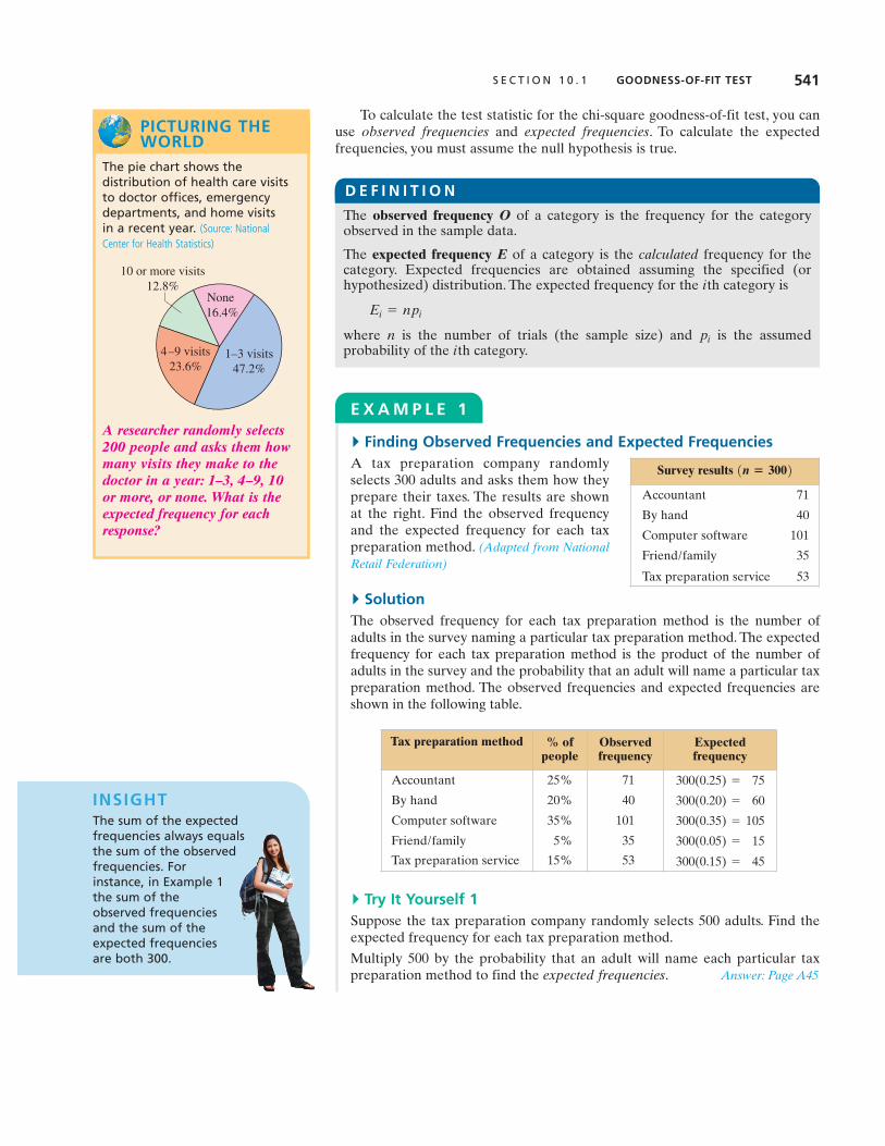
7. Ages of Moviegoers Results from a previous survey asking people who go to movies at least once a month for their ages are shown in the graph. Todetermine whether this distribution is still the same, you randomly select 1000people who go to movies at least once a month and record the age of each.Theresults are shown in the table. At are the distributions the same?(Source: Motion Picture Association of America)
8. Coffee Results from a previous survey asking coffee drinkers how much coffee they drink are shown in the graph. To determine whether this distribution is still the same, you randomly select 1600 coffee drinkers and askthem how much coffee they drink. The results are shown in the table.At are the distributions the same? (Source: Braun Research)
Survey results
Response Frequency, f
2 cups a week 206
1 cup a week 193
1 cup a day 4622 or more cups a day 739
How many cups-o-joedo you drink?About 72% of Americans drink coffee.How much they drink:
1 cup a day27%
2 or morecups a day
45%
1 cup a week13%
2 cupsa week15%
a = 0.05,
Survey results
Age Frequency, f
2–17 240
18–24 214
25–39 183
40–49 15650+ 207
How old are moviegoers?Age of those who go to moviesonce a monthor more
26.7%19.8%
19.7%
14%19.8%50+
2-17
18-24
25-39
40-49
a = 0.10,
Ha ,H0
pi = 0.08n = 415,pi = 0.25n = 230,
pi = 0.9n = 500,pi = 0.3n = 150,
pi .
546 C H A P T E R 1 0 CHI-SQUARE TESTS AND THE F -DISTRIBUTION
10.1 EXERCISES

S E C T I O N 1 0 . 1 GOODNESS-OF-FIT TEST 547
9. Ordering Delivery Results from a previous survey asking people which dayof the week they are most likely to order food for delivery are shown in thegraph. To determine whether this distribution has changed, you randomlyselect 500 people and record which day of the week each is most likely toorder food for delivery. The results are shown in the table. At canyou conclude that there has been a change in the claimed or expected distribution? (Source: Technomic, Inc.)
10. Reasons Workers Leave A personnel director believes that the distributionof the reasons workers leave their jobs is different from the one shown in thegraph. The director randomly selects 200 workers who recently left their jobsand records each worker’s reason for doing so. The results are shown in thetable. At are the distributions different? (Source: Robert HalfInternational, Inc.)
11. Homicides by Season A researcher believes that the number of homicidecrimes in California by season is uniformly distributed.To test this claim, yourandomly select 1200 homicides from a recent year and record the seasonwhen each happened. The results are shown in the table. At canyou reject the claim that the distribution is uniform? (Adapted from CaliforniaDepartment of Justice)
Season Frequency, f
Spring 312
Summer 299
Fall 297
Winter 292
a = 0.05,
Survey results
Response Frequency, f
Limited advancementpotential 78
Lack of recognition 52
Low salary/benefits 30
Unhappy with mgmt. 25Bored/don’t know 15
Why workers leaveReasons given for goodemployees quitting their jobs:
41%Limitedadvance-mentpotential
25%Lack ofrecognition
15%Low salary/benefits 10%
Unhappy withmanagement
9%Bored/don't know
a = 0.01,
Survey results
Day Frequency, f
Sunday 43
Monday 16
Tuesday 25
Wednesday 49
Thursday 46
Friday 168Saturday 153
Food at your doorDay of the week Americansare most likely to orderfood for delivery:
10%
36%
24%7%4%6%
13%Wednesday
Friday
SaturdaySunday
MondayTuesday
Thursday
a = 0.01,

12. Homicides by Month A researcher believes that the number of homicidecrimes in California by month is uniformly distributed. To test this claim, yourandomly select 1200 homicides from a recent year and record the monthwhen each happened. The results are shown in the table. At canyou reject the claim that the distribution is uniform? (Adapted from CaliforniaDepartment of Justice)
13. College Education The pie chart shows the distribution of the opinions of U.S. parents on whether a college education is worth the expense. Aneconomist believes that the distribution of the opinions of U.S. teenagers isdifferent from the distribution for U.S. parents. The economist randomlyselects 200 U.S. teenagers and asks each whether a college education is worth the expense. The results are shown in the table. At are thedistributions different? (Adapted from Upromise, Inc.)
14. Saving for the Future The pie chart shows the distribution of the opinionsof U.S. male adults on which is more important to save for, your child’s college education or your own retirement. A financial services companybelieves that the distribution of the opinions of U.S. female adults is the sameas the distribution for U.S. male adults. The company randomly selects 400 U.S. female adults and asks each which is more important—saving foryour child’s college education or saving for your own retirement. The resultsare shown in the table.At are the distributions the same? (Adaptedfrom Country Financial)
Survey results
Response Frequency, f
Saving for your child’s college education 180
Saving for your own retirement 172
Not sure 48
Saving for yourchild’s college
education50%
Saving foryour ownretirement
37%
Not sure13%
a = 0.10,
Survey results
Response Frequency, f
Strongly agree 86
Somewhat agree 62
Neither agree nor disagree 34
Somewhat disagree 14Strongly disagree 4
Neither agreenor disagree
5%
Somewhat disagree6% Strongly
disagree4%
Somewhatagree30%
Stronglyagree55%
a = 0.05,
Month Frequency, f Month Frequency, f
January 98 July 84
February 103 August 109
March 114 September 112
April 92 October 95
May 106 November 91
June 106 December 90
a = 0.10,
548 C H A P T E R 1 0 CHI-SQUARE TESTS AND THE F -DISTRIBUTION

S E C T I O N 1 0 . 1 GOODNESS-OF-FIT TEST 549
15. Home Sizes An organization believes that the number of prospective homebuyers who want their next house to be larger, smaller, or the same size astheir current house is uniformly distributed. To test this claim, you randomlyselect 800 prospective home buyers and ask them what size they want theirnext house to be. The results are shown in the table. At can youreject the claim that the distribution is uniform? (Adapted from Better Homesand Gardens)
16. Births by Day of the Week A doctor believes that the number of births byday of the week is uniformly distributed. To test this claim, you randomlyselect 700 births from a recent year and record the day of the week on whicheach takes place.The results are shown below.At can you reject theclaim that the distribution is uniform? (Adapted from National Center for HealthStatistics)
In Exercises 17 and 18, use StatCrunch to perform a chi-square goodness-of-fittest. Decide whether to reject the null hypothesis. Then, interpret the decision in thecontext of the original claim.
17. Favorite Sport Results from a survey five years ago asking U.S. adults their favorite sport are shown in the pie chart. To determine whether this distribution has changed, a research organization randomly selects 400 U.S.adults and records each adult’s favorite sport. The results are shown in thetable. At can you conclude that there has been a change in theclaimed or expected distribution? (Adapted from Harris Interactive)
Survey results
Sport Frequency, f
Auto racing 36
Baseball 64
College basketball 12
College football 48
Golf 16
Hockey 16
Other/not sure 40
Pro basketball 20
Pro football 140Soccer 8
Baseball15%
Golf4%Hockey
4%
Soccer3%
Other/not sure
13%
Collegebasketball
6%Pro
basketball7%
Collegefootball
11%
Profootball
30%
Auto racing7%
a = 0.10,
SC
Day Frequency, f
Sunday 65
Monday 103
Tuesday 114
Wednesday 116
Thursday 115
Friday 112Saturday 75
a = 0.01,
Response Frequency, f
Larger 285
Same size 224Smaller 291
a = 0.05,

18. Paying Bills The pie chart shows the distribution of the opinions of U.S.adults who are married on how long they could go between jobs without anyincome and still be able to pay all of their bills on time.A researcher believesthat the distribution of the opinions of U.S. adults who are not married is different from the distribution for U.S. adults who are married. Theresearcher randomly selects 250 U.S. adults who are not married and asksthem how long they could go between jobs without any income and still beable to pay all of their bills on time. The results are shown in the table. At
are the distributions different? (Adapted from Country Financial)
# EXTENDING CONCEPTSTesting for Normality Using a chi-square goodness-of-fit test, you can decide,with some degree of certainty, whether a variable is normally distributed. In all chi-square tests for normality, the null and alternative hypotheses are as follows.
The variable has a normal distribution.The variable does not have a normal distribution.
To determine the expected frequencies when performing a chi-square test fornormality, first find the mean and standard deviation of the frequency distribution.Then, use the mean and standard deviation to compute the z-score for each classboundary. Then, use the z-scores to calculate the area under the standard normalcurve for each class. Multiplying the resulting class areas by the sample size yieldsthe expected frequency for each class.
In Exercises 19 and 20, (a) find the expected frequencies, (b) find the critical valueand identify the rejection region, (c) find the chi-square test statistic, (d) decidewhether to reject or fail to reject the null hypothesis, and (e) interpret the decisionin the context of the original claim.
19. Test Scores The frequency distribution shows the results of 200 test scores.Are the test scores normally distributed? Use
20. Test Scores At test the claim that the 400 test scores shown in thefrequency distribution are normally distributed.
Class boundaries 50.5–60.5 60.5–70.5 70.5–80.5 80.5–90.5 90.5–100.5
Frequency, f 28 106 151 97 18
a = 0.05,
Class boundaries 49.5–58.5 58.5–67.5 67.5–76.5 76.5–85.5 85.5–94.5
Frequency, f 19 61 82 34 4
a = 0.01.
Ha:H0:
Survey results
Response Frequency, f
None 83
One month 46
Two months 37
Three months 11
Four months 9
Five months 7
More than fivemonths 52
Not sure 5
None33%
One month15%
Not sure2%
Two months11%
Three months7%
Four months4%
Five months3%
More thanfive months
25%
a = 0.01,
550 C H A P T E R 1 0 CHI-SQUARE TESTS AND THE F -DISTRIBUTION

S E C T I O N 1 0 . 2 INDEPENDENCE 551
" CONTINGENCY TABLESIn Section 3.2, you learned that two events are independent if the occurrence ofone event does not affect the probability of the occurrence of the other event. Forinstance, the outcomes of a roll of a die and a toss of a coin are independent. But,suppose a medical researcher wants to determine if there is a relationshipbetween caffeine consumption and heart attack risk. Are these variablesindependent or are they dependent? In this section, you will learn how to use thechi-square test for independence to answer such a question. To perform a chi-square test for independence, you will use sample data that are organized ina contingency table.
For instance, the following table is a contingency table. It has two rows andfive columns and shows the results of a random sample of 2200 adults classifiedby their favorite way to eat ice cream and gender. From the table, you can seethat 204 of the adults who prefer ice cream in a sundae are males, and 180 of theadults who prefer ice cream in a sundae are females.
Assuming the two variables of study in a contingency table are independent, youcan use the contingency table to find the expected frequency for each cell. Theformula for calculating the expected frequency for each cell is given below.
When you find the sum of each row and column in a contingency table, you are calculating the marginal frequencies. A marginal frequency is the frequencythat an entire category of one of the variables occurs. For instance, in the tableabove, the marginal frequency for adults who prefer ice cream in a cone is
The observed frequencies in the interior of a contingency table are called joint frequencies. The marginal frequencies for the contingency table in Example 1 have already been calculated.
288 + 340 = 628.
2 * 5
Contingency Tables " The Chi-Square Test for Independence
" How to use a contingencytable to find expected frequencies
" How to use a chi-squaredistribution to test whether two variables are independent
10.2 Independence
WHAT YOU SHOULD LEARN
An contingency table shows the observed frequencies for two variables.The observed frequencies are arranged in r rows and c columns. The intersection of a row and a column is called a cell.
r : cD E F I N I T I O N
The expected frequency for a cell in a contingency table is
Expected frequency Er, c =1Sum of row r2 * 1Sum of column c2
Sample size.
Er, c
F I N D I N G T H E E X P E C T E D F R E Q U E N C Y F O RC O N T I N G E N C Y TA B L E C E L L S
STUDY TIPIn a contingency table, the notation represents the expected frequency for the cell in row r,column c. For instance, in the table above, represents the expected frequency for the cell in row 1, column 4.
E1, 4
Er, c
Favorite way to eat ice cream
Gender Cup Cone Sundae Sandwich Other
Male 600 288 204 24 84
Female 410 340 180 20 50
(Adapted from Harris Interactive)

552 C H A P T E R 1 0 CHI-SQUARE TESTS AND THE F -DISTRIBUTION
E X A M P L E 1
!Finding Expected FrequenciesFind the expected frequency for each cell in the contingency table. Assumethat the variables, favorite way to eat ice cream and gender, are independent.
!SolutionAfter calculating the marginal frequencies, you can use the formula
to find each expected frequency as shown.
!Try It Yourself 1The marketing consultant for a travel agency wants to determine whether certain travel concerns are related to travel purpose. The contingency tableshows the results of a random sample of 300 travelers classified by their primary travel concern and travel purpose. Assume that the variables travelconcern and travel purpose are independent. Find the expected frequency foreach cell. (Adapted from NPD Group for Embassy Suites)
a. Calculate the marginal frequencies.b. Determine the sample size.c. Use the formula to find the expected frequency for each cell.
Answer: Page A46
E2, 5 = 1000 # 1342200
L 60.91E2, 4 = 1000 # 442200
= 20
E2, 3 = 1000 # 3842200
L 174.55E2, 2 = 1000 # 6282200
L 285.45
E2, 1 = 1000 # 10102200
L 459.09E1, 5 = 1200 # 1342200
L 73.09
E1, 4 = 1200 # 442200
= 24E1, 3 = 1200 # 3842200
L 209.45
E1, 2 = 1200 # 6282200
L 342.55E1, 1 = 1200 # 10102200
L 550.91
Expected frequency Er, c =1Sum of row r2 * 1Sum of column c2
Sample size
INSIGHTIn Example 1, once the expectedfrequency for has been calculated to be 550.91, you can determine the expected frequency for to be
That is, the expected frequency for the last cell in each row or column can be found by subtracting from the total.
1010 - 550.91 = 459.09 .E2, 1
E1, 1
Travel concern
Travelpurpose
Hotelroom
Leg roomon plane
Rentalcar size Other
Business 36 108 14 22
Leisure 38 54 14 14
Favorite way to eat ice cream
Gender Cup Cone Sundae Sandwich Other Total
Male 600 288 204 24 84 1200
Female 410 340 180 20 50 1000
Total 1010 628 384 44 134 2200

S E C T I O N 1 0 . 2 INDEPENDENCE 553
" THE CHI-SQUARE TEST FOR INDEPENDENCEAfter finding the expected frequencies, you can test whether the variables areindependent using a chi-square independence test.
For the chi-square independence test to be used, the following conditionsmust be true.
1. The observed frequencies must be obtained using a random sample.2. Each expected frequency must be greater than or equal to 5.
To begin the independence test, you must first state a null hypothesis and analternative hypothesis. For a chi-square independence test, the null and alternativehypotheses are always some variation of the following statements.
The variables are independent.
The variables are dependent.
The expected frequencies are calculated on the assumption that the two variables are independent. If the variables are independent, then you can expectlittle difference between the observed frequencies and the expected frequencies.When the observed frequencies closely match the expected frequencies, thedifferences between O and E will be small and the chi-square test statistic will beclose to 0. As such, the null hypothesis is unlikely to be rejected.
However, if the variables are dependent, there will be large discrepanciesbetween the observed frequencies and the expected frequencies. When thedifferences between O and E are large, the chi-square test statistic is also large.A large chi-square test statistic is evidence for rejecting the null hypothesis. So,the chi-square independence test is always a right-tailed test.
Ha:
H0:
PICTURING THEWORLD
A researcher wants to determinewhether a relationship existsbetween where people work(workplace or home) and theireducational attainment. Theresults of a random sample of925 employed persons are shownin the contingency table. (Adaptedfrom U.S. Bureau of Labor Statistics)
Can the researcher use this sample to test for independenceusing a chi-square independencetest? Why or why not?
A chi-square independence test is used to test the independence of two variables. Using a chi-square test, you can determine whether the occurrenceof one variable affects the probability of the occurrence of the other variable.
D E F I N I T I O N
If the conditions listed above are satisfied, then the sampling distribution forthe chi-square independence test is approximated by a chi-square distributionwith
degrees of freedom, where r and c are the number of rows and columns,respectively, of a contingency table. The test statistic for the chi-square independence test is
where O represents the observed frequencies and E represents the expectedfrequencies.
x2 = g 1O - E22E
1r - 121c - 12T H E C H I - S Q U A R E I N D E P E N D E N C E T E S T
Where they work
Educationalattainment Workplace Home
Less thanhigh school
35 2
High schooldiploma
250 21
Some college
226 30
BA degree or higher
293 68

554 C H A P T E R 1 0 CHI-SQUARE TESTS AND THE F -DISTRIBUTION
E X A M P L E 2
!Performing a Chi-Square Independence TestThe contingency table shows the results of a random sample of 2200 adultsclassified by their favorite way to eat ice cream and gender. The expected frequencies are displayed in parentheses. At can you conclude thatthe adults’ favorite ways to eat ice cream are related to gender?
!SolutionThe expected frequencies were calculated in Example 1. Because each expectedfrequency is at least 5 and the adults were randomly selected, you can use thechi-square independence test to test whether the variables are independent.The null and alternative hypotheses are as follows.
The adults’ favorite ways to eat ice cream are independent of gender.
The adults’ favorite ways to eat ice cream are dependent on gender.(Claim)
Ha:
H0:
a = 0.01,
Performing a Chi-Square Test for IndependenceIN WORDS IN SYMBOLS
1. Identify the claim. State the null and State and alternative hypotheses.
2. Specify the level of significance. Identify
3. Determine the degrees of freedom.
4. Determine the critical value. Use Table 6 in Appendix B.
5. Determine the rejection region.
6. Find the test statistic and sketch the sampling distribution.
7. Make a decision to reject or fail to If is in the rejection reject the null hypothesis. region, reject Other-
wise, fail to reject
8. Interpret the decision in the contextof the original claim.
H0.H0 .
x2
x2 = g 1O - E22E
d.f. = 1r - 121c - 12a .
Ha .H0
G U I D E L I N E S
STUDY TIPA contingency table withthree rows and four columns will have
= 6 d.f.
13 - 1214 - 12 = 122132
SC
Favorite way to eat ice cream
Gender Cup Cone Sundae Sandwich Other Total
Male 600(550.91)
288(342.55)
204(209.45)
24(24)
84(73.09)
1200
Female 410(459.09)
340(285.45)
180(174.55)
20(20)
50(60.91)
1000
Total 1010 628 384 44 134 2200
Report 47
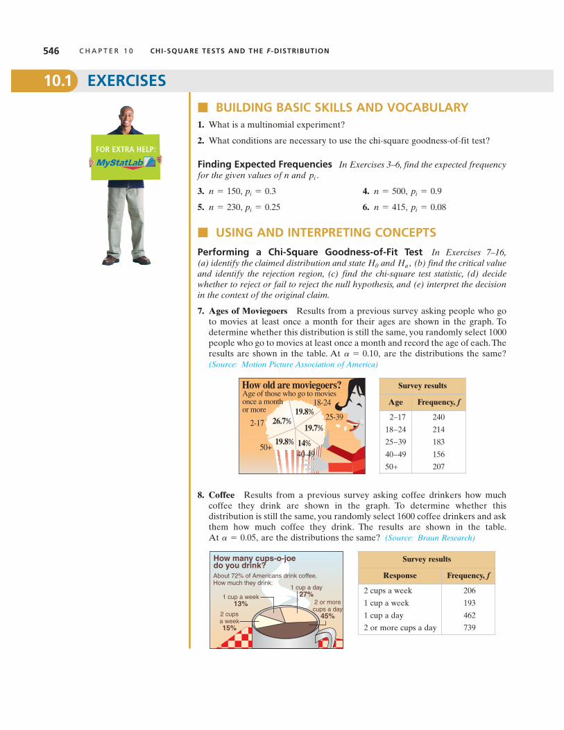
S E C T I O N 1 0 . 2 INDEPENDENCE 555
Because the contingency table has two rows and five columns, the chi-squaredistribution has degrees of freedom.Because and the critical value is With theobserved and expected frequencies, the chi-square test statistic is as shown.
The graph at the left shows the location of the rejection region. Becauseis in the rejection region, you should decide to reject the null
hypothesis.Interpretation There is enough evidence at the 1% level of significance to conclude that the adults’ favorite ways to eat ice cream and gender are dependent.
!Try It Yourself 2The marketing consultant for a travel agency wants to determine whether travel concerns are related to travel purpose. The contingency table shows theresults of a random sample of 300 travelers classified by their primary travelconcern and travel purpose. At can the consultant conclude that thetravel concerns depend on the purpose of travel? (The expected frequenciesare displayed in parentheses.) (Adapted from NPD Group for Embassy Suites)
a. Identify the claim and state and b. Specify the level of significancec. Determine the degrees of freedom.d. Determine the critical value and the rejection region.e. Use the observed and expected frequencies to find the chi-square test statistic.
Sketch a graph.f. Decide whether to reject the null hypothesis.g. Interpret the decision in the context of the original claim.
Answer: Page A46
a .Ha .H0
a = 0.01,
x2 L 32.630
x20 = 13.277.a = 0.01,d.f. = 4
1r - 121c - 12 = 12 - 1215 - 12 = 4
5 10 15 20 25
02χ = 13.277
α = 0.01
Rejectionregion
2χ
Travel concern
Travelpurpose
Hotelroom
Leg roomon plane
Rentalcar size Other Total
Business 36 (44.4) 108 (97.2) 14 (16.8) 22 (21.6) 180
Leisure 38 (29.6) 54 (64.8) 14 (11.2) 14 (14.4) 120
Total 74 162 28 36 300
O E O " E 1O " E22 1O " E22E
600 550.91 49.09 2409.8281 4.3743
288 342.55 -54.55 2975.7025 8.6869
204 209.45 -5.45 29.7025 0.1418
24 24 0 0 0
84 73.09 10.91 119.0281 1.6285
410 459.09 -49.09 2409.8281 5.2491
340 285.45 54.55 2975.7025 10.4246
180 174.55 5.45 29.7025 0.1702
20 20 0 0 0
50 60.91 -10.91 119.0281 1.9542
x2 = g 1O - E22E
L 32.630

556 C H A P T E R 1 0 CHI-SQUARE TESTS AND THE F -DISTRIBUTION
E X A M P L E 3
!Using Technology for a Chi-Square Independence TestA health club manager wants to determine whether the number of days perweek that college students spend exercising is related to gender. A randomsample of 275 college students is selected and the results are classified asshown in the table. At is there enough evidence to conclude that the number of days spent exercising per week is related to gender?
!Solution The null and alternative hypotheses can be stated as follows.
The number of days spent exercising per week is independent of gender.The number of days spent exercising per week depends on gender. (Claim)
Using a TI-83/84 Plus, enter the observed frequencies into Matrix A and theexpected frequencies into Matrix B, making sure that each expected frequencyis greater than or equal to 5. To perform a chi-square independence test,begin with the STAT keystroke and choose the TESTS menu and select
Then set up the chi-square test as shown in the top-left screen.The other displays at the left show the results of selecting Calculate or
Draw. Because and the critical value is So,the rejection region is The test statistic is not in the rejection region, so you should fail to reject the null hypothesis.Interpretation There is not enough evidence to conclude that the number ofdays spent exercising per week is related to gender.
!Try It Yourself 3A researcher wants to determine if age is related to whether or not a tax cutwould influence an adult to purchase a hybrid vehicle. A random sample of1250 adults is selected and the results are classified as shown in the table. At
is there enough evidence to conclude that the adults’ ages are related to the response? (Adapted from HNTB)
a. Identify the claim and state and b. Use a technology tool to enter the observed and expected frequencies into
matrices.c. Determine the critical value and the rejection region.d. Use the technology tool to find the chi-square test statistic.e. Decide whether to reject the null hypothesis. Use a graph if necessary.f. Interpret the decision in the context of the original claim.
Answer: Page A46
Ha.H0
a = 0.01,
x2 L 3.493x 2 7 7.815.x0
2 = 7.815.a = 0.05,d.f. = 3
C: x2 - Test.
Ha:H0:
a = 0.05,
STUDY TIPYou can also use a P-value to perform a chi-square test for independence. For instance, in Example 3, note that the TI-83/84 Plus displays
Becauseyou should fail
to reject the null hypothesis.
P 7 a,P = .321624691 .
T I - 8 3 / 8 4 PLUS
2=3.4934 p=.3216χ
Age
Response 18–34 35–54 55 and older Total
Yes 257 189 143 589
No 218 261 182 661
Total 475 450 325 1250
Days per week spent exercising
Gender 0–1 2–3 4–5 6–7 Total
Male 40 53 26 6 125
Female 34 68 37 11 150
Total 74 121 63 17 275
T I - 8 3 / 8 4 PLUS
–TestObserved: [A]Expected: [B]Calculate Draw
x2
T I - 8 3 / 8 4 PLUS
–Test
=3.493357223p=.321624691df=3
x2
x2
Rating
Size of restaurant Excellent Fair Poor
Seats 100 or fewer 182 203 165
Seats over 100 180 311 159
Preference
Bank employee New procedure Old procedure No preference
Teller 92 351 50
Customer servicerepresentative
76 42 8
Treatment
Result Drug Placebo
Nausea 36 13
No nausea 254 262
Athlete has
Result Stretched Not stretched
Injury 18 22
No injury 211 189
S E C T I O N 1 0 . 2 INDEPENDENCE 557
# BUILDING BASIC SKILLS AND VOCABULARY1. Explain how to find the expected frequency for a cell in a contingency table.
2. Explain the difference between marginal frequencies and joint frequenciesin a contingency table.
3. Explain how the chi-square test for independence and the chi-square goodness-of-fit test are similar. How are they different?
4. Explain why the chi-square independence test is always a right-tailed test.
True or False? In Exercises 5 and 6, determine whether the statement is true orfalse. If it is false, rewrite it as a true statement.
5. If the two variables of the chi-square test for independence are dependent,then you can expect little difference between the observed frequencies andthe expected frequencies.
6. If the test statistic for the chi-square independence test is large, you will, inmost cases, reject the null hypothesis.
Finding Expected Frequencies In Exercises 7–12, (a) calculate the marginalfrequencies, and (b) find the expected frequency for each cell in the contingencytable. Assume that the variables are independent.
7.
8.
9.
10.
10.2 EXERCISES

Age
Type of movierented 18–24 25–34 35–44 45–64 65 and older
Comedy 38 30 24 10 8
Action 15 17 16 9 5
Drama 12 11 19 25 13
Type of car
Gender Compact Full-size SUV Truck/van
Male 28 39 21 22
Female 24 32 20 14
11.
12.
# USING AND INTERPRETING CONCEPTSPerforming a Chi-Square Test for Independence In Exercises 13–22,perform the indicated chi-square test for independence by doing the following.
(a) Identify the claim and state the null and alternative hypotheses.
(b) Determine the degrees of freedom, find the critical value, and identify the rejection region.
(c) Calculate the test statistic. If convenient, use technology.
(d) Decide to reject or fail to reject the null hypothesis. Then interpret the decisionin the context of the original claim.
13. Achievement and School Location Is achieving a basic skill level in a subject related to the location of the school? The results of a random sampleof students by the location of school and the number of those studentsachieving basic skill levels in three subjects is shown in the contingencytable. At test the hypothesis that the variables are independent.(Adapted from HUD State of the Cities Report)
14. Attitudes about Safety The results of a random sample of students by typeof school and their attitudes on safety steps taken by the school staff areshown in the contingency table. At can you conclude that attitudesabout the safety steps taken by the school staff are related to the type ofschool? (Adapted from Horatio Alger Association)
a = 0.01,
a = 0.01,
558 C H A P T E R 1 0 CHI-SQUARE TESTS AND THE F -DISTRIBUTION
Subject
Location of school Reading Math Science
Urban 43 42 38
Suburban 63 66 65
School staff has
Type ofschool
Taken all steps necessaryfor student safety
Taken some stepstoward student safety
Public 40 51
Private 64 34

S E C T I O N 1 0 . 2 INDEPENDENCE 559
15. Trying to Quit Smoking The contingency table shows the number of timesa random sample of former smokers tried to quit smoking before they werehabit-free and gender. At can you conclude that the number oftimes they tried to quit before they were habit-free is related to gender?(Adapted from Porter Novelli Health Styles for the American Lung Association)
16. Reviewing a Movie The contingency table shows how a random sample ofadults rated a newly released movie and gender. At can you conclude that the adults’ ratings are related to gender?
17. Obsessive-Compulsive Disorder The results of a random sample of patientswith obsessive-compulsive disorder treated with a drug or with a placebo areshown in the contingency table. At can you conclude that the treatment is related to the result? On the basis of these results, would yourecommend using the drug as part of a treatment for obsessive-compulsivedisorder? (Adapted from The Journal of the American Medical Association)
18. Musculoskeletal Injury The results of a random sample of children withpain from musculoskeletal injuries treated with acetaminophen, ibuprofen,or codeine are shown in the contingency table.At can you concludethat the treatment is related to the result? (Adapted from American Academy of Pediatrics)
a = 0.10,
a = 0.10,
a = 0.05,
a = 0.05,
Number of times tried to quit before habit-free
Gender 1 2–3 4 or more
Male 271 257 149
Female 146 139 80
Rating
Gender Excellent Good Fair Poor
Male 97 42 26 5
Female 101 33 25 11
Treatment
Result Acetaminophen Ibuprofen Codeine
Significant improvement 58 81 61
Slight improvement 42 19 39
Treatment
Result Drug Placebo
Improvement 39 25
No change 54 70

19. Continuing Education You work for a college’s continuing educationdepartment and want to determine whether the reasons given by workers for continuing their education are related to job type. In your study, you randomly collect the data shown in the contingency table. At canyou conclude that the reason and the type of worker are dependent? Howcould you use this information in your marketing efforts? (Adapted fromMarket Research Institute for George Mason University)
20. Ages and Goals You are investigating the relationship between the ages ofU.S. adults and what aspect of career development they consider to be themost important. You randomly collect the data shown in the contingencytable. At is there enough evidence to conclude that age is relatedto which aspect of career development is considered to be most important?(Adapted from Harris Interactive)
21. Vehicles and Crashes You work for an insurance company and are studying the relationship between types of crashes and the vehicles involved in passenger vehicle occupant deaths. As part of your study, yourandomly select 4270 vehicle crashes and organize the resulting data asshown in the contingency table. At can you conclude that the typeof crash depends on the type of vehicle? (Adapted from Insurance Institute forHighway Safety)
22. Library Internet Access Speed The contingency table shows a random sample of urban, suburban, and rural libraries and the speed of their Internetaccess. In the table, mbps represents megabits per second. At canyou conclude that the metropolitan status of libraries and Internet accessspeed are related? (Adapted from Center for Library and Information Innovation)
a = 0.01,
a = 0.05,
a = 0.01,
a = 0.01,
560 C H A P T E R 1 0 CHI-SQUARE TESTS AND THE F -DISTRIBUTION
Reason
Type of worker Professional Personal Professional and personal
Technical 30 36 41
Other 47 25 30
Vehicle
Type of crash Car Pickup Sport utility
Single-vehicle 1237 547 479
Multiple-vehicle 1453 307 247
Career development aspect
Age Learning new skills Pay increases Career path
18–26 years 31 22 21
27–41 years 27 31 33
42–61 years 19 14 8
Metropolitan status
Access speed Urban Suburban Rural
1.4 mbps or less 5 20 58
1.5 mbps – 3.0 mbps 24 46 65
Greater than 3.0 mbps 37 59 64

S E C T I O N 1 0 . 2 INDEPENDENCE 561
In Exercises 23 and 24, use StatCrunch to (a) find the marginal frequencies,(b) find the expected frequencies for each cell in the contingency table, and (c) perform the indicated chi-square test for independence.
23. Financing and Education A financial aid officer is studying the relationshipbetween family decisions to borrow money to finance their child’s educationand their child’s expected income after graduation. As part of the study, 440families are randomly selected and the resulting data are organized as shownin the contingency table. At can you conclude that the decision toborrow money is related to the child’s expected income after graduation?(Adapted from Sallie Mae, Inc.)
24. Alcohol-Related Accidents The contingency table shows the results of arandom sample of fatally injured passenger vehicle drivers (with blood alcohol concentrations greater than or equal to 0.08) by age and gender.At can you conclude that age is related to gender in such alcohol-related accidents? (Adapted from Insurance Institute for Highway Safety)
# EXTENDING CONCEPTSHomogeneity of Proportions Test In Exercises 25–28, use the followinginformation. Another chi-square test that involves a contingency table is the homogeneity of proportions test. This test is used to determine if several proportions are equal when samples are taken from different populations. Beforethe populations are sampled and the contingency table is made, the sample sizesare determined. After randomly sampling different populations, you can testwhether the proportion of elements in a category is the same for each populationusing the same guidelines in performing a chi-square independence test. The nulland alternative hypotheses are always some variation of the following statements.
The proportions are equal.
At least one of the proportions is different from the others.
Performing a homogeneity of proportions test requires that the observed frequencies be obtained using a random sample, and each expected frequency mustbe greater than or equal to 5.
Ha:
H0:
a = 0.05,
a = 0.01,
SC
Age
Gender 16–20 21–30 31–40 41–50 51–60 61 and older
Male 45 170 90 72 45 26
Female 9 30 21 17 10 5
Impact on decision to borrow money
Expected incomeMorelikely
Lesslikely
Did notmake a
difference
Did notconsider
it
Less than $35,000 37 10 22 25
$35,000–$50,000 28 12 15 16
$50,000–$100,000 55 9 65 48
Greater than $100,000 36 1 29 32
25. Motor Vehicle Crash Deaths The contingency table shows the results of arandom sample of motor vehicle crash deaths by age and gender. At
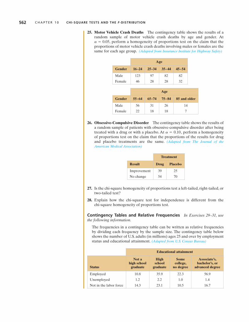
perform a homogeneity of proportions test on the claim that theproportions of motor vehicle crash deaths involving males or females are thesame for each age group. (Adapted from Insurance Institute for Highway Safety)
26. Obsessive-Compulsive Disorder The contingency table shows the results ofa random sample of patients with obsessive-compulsive disorder after beingtreated with a drug or with a placebo. At perform a homogeneityof proportions test on the claim that the proportions of the results for drugand placebo treatments are the same. (Adapted from The Journal of theAmerican Medical Association)
27. Is the chi-square homogeneity of proportions test a left-tailed, right-tailed, ortwo-tailed test?
28. Explain how the chi-square test for independence is different from the chi-square homogeneity of proportions test.
Contingency Tables and Relative Frequencies In Exercises 29–31, usethe following information.
The frequencies in a contingency table can be written as relative frequenciesby dividing each frequency by the sample size. The contingency table belowshows the number of U.S. adults (in millions) ages 25 and over by employmentstatus and educational attainment. (Adapted from U.S. Census Bureau)
a = 0.10,
a = 0.05,
562 C H A P T E R 1 0 CHI-SQUARE TESTS AND THE F -DISTRIBUTION
Age
Gender 16–24 25–34 35–44 45–54
Male 123 97 82 82
Female 46 28 28 32
Age
Gender 55–64 65–74 75–84 85 and older
Male 56 31 26 14
Female 22 18 18 7
Treatment
Result Drug Placebo
Improvement 39 25
No change 54 70
Educational attainment
Status
Not a high school
graduate
High school
graduate
Some college,
no degree
Associate’s,bachelor’s, or
advanced degree
Employed 10.8 35.9 22.3 56.9
Unemployed 1.2 2.2 1.0 1.4
Not in the labor force 14.3 23.1 10.5 16.7

S E C T I O N 1 0 . 2 INDEPENDENCE 563
29. Rewrite the contingency table using relative frequencies.
30. What percent of U.S. adults ages 25 and over
(a) have a degree and are unemployed?(b) have some college education, but no degree, and are not in the labor
force?(c) are employed and high school graduates?(d) are not in the labor force?(e) are high school graduates?
31. Explain why you cannot perform the chi-square independence test on thesedata.
Conditional Relative Frequencies In Exercises 32–39, use the contingencytable from Exercises 29–31, and the following information.
Relative frequencies can also be calculated based on the row totals (by dividing each row entry by the row’s total) or the column totals (by dividingeach column entry by the column’s total). These frequencies are conditional relative frequencies and can be used to determine if an association existsbetween two categories in a contingency table.
32. Calculate the conditional relative frequencies in the contingency table basedon the row totals.
33. What percent of U.S. adults ages 25 and over who are employed have adegree?
34. What percent of U.S. adults ages 25 and over who are not in the labor forcehave some college education, but no degree?
35. Calculate the conditional relative frequencies in the contingency table basedon the column totals.
36. What percent of U.S. adults ages 25 and over who have a degree are not inthe labor force?
37. What percent of U.S. adults ages 25 and over who are not high school graduates are unemployed?
38. Use your results from Exercise 35 to construct a bar graph that shows thepercentages of U.S. adults ages 25 and over based on employment status.Each category of employment status will have four bars, representing thefour levels of educational attainment mentioned in the contingency table.
39. What conclusions can you make from the bar graph you constructed inExercise 38?

564 C H A P T E R 1 0 CHI-SQUARE TESTS AND THE F -DISTRIBUTIONC
AS
ES
TU
DY
# EXERCISES1. Assuming the variables gender and response
are independent, did female respondents ormale respondents exceed the expected number of “somewhat agree” responses?
2. Assuming the variables gender and responseare independent, did female respondents ormale respondents exceed the expected numberof “neither agree nor disagree” responses?
3. At perform a chi-square indepen-dence test to determine whether the variablesresponse and gender are independent. Whatcan you conclude?
In Exercises 4 and 5, perform a chi-square goodness-of-fit test to compare the national distribution of responses with the distribution ofeach gender. Use the national distribution as theclaimed distribution. Use 0.05.
4. Compare the distribution of responses byfemales with the national distribution. Whatcan you conclude?
5. Compare the distribution of responses bymales with the national distribution. What canyou conclude?
6. In addition to the variables used in the CaseStudy, what other variables do you think areimportant to consider when studying the distribution of U.S. consumers’ attitudes abouthealthy fast food?
a =
a = 0.01,
With the growing trend toward healthier eating, fast food chains are revising their menus. Some chainshave added healthier options, such as salads, while other chains are grilling foods instead of frying them.QSR Magazine conducted a recent survey of 673 U.S. consumers regarding their attitudes and preferences about fast food.
One question in the survey asks:Do you agree that, on the whole, fast food menus have gotten healthier over the past 3 years?
The pie chart shows the response to the question on a national level. The contingency table shows theresults classified by gender and response.
Fast Food Survey
Are Fast FoodMenus Healthier?
Somewhat agree59%
Neitheragree nordisagree
20%
Stronglyagree12%
Disagree 9%
Gender
Response Female Male
Somewhat agree 286 114
Neither agree nor disagree 76 58
Strongly agree 62 19
Disagree 34 24

S E C T I O N 1 0 . 3 COMPARING TWO VARIANCES 565
" THE F-DISTRIBUTIONIn Chapter 8, you learned how to perform hypothesis tests to comparepopulation means and population proportions. Recall from Section 8.2 that thet-test for the difference between two population means depends on whether thepopulation variances are equal. To determine whether the population variancesare equal, you can perform a two-sample F-test.
In this section, you will learn about the F-distribution and how it can be usedto compare two variances.
The F-Distribution " The Two-Sample F-Test for Variances
" How to interpret the F-distribution and use an F-table to find critical values
" How to perform a two-sampleF-test to compare twovariances
10.3 Comparing Two Variances
WHAT YOU SHOULD LEARN
Let and represent the sample variances of two different populations.If both populations are normal and the population variances and areequal, then the sampling distribution of
is called an F-distribution. Several properties of the F-distribution are as follows.
1. The F-distribution is a family of curves each of which is determined by twotypes of degrees of freedom: the degrees of freedom corresponding to thevariance in the numerator, denoted by and the degrees of freedomcorresponding to the variance in the denominator, denoted by
2. F-distributions are positively skewed.3. The total area under each curve of an F-distribution is equal to 1.4. F-values are always greater than or equal to 0.5. For all F-distributions, the mean value of F is approximately equal to 1.
F-Distributions
F
d.f.N = 1 and d.f.D = 8
d.f.N = 3 and d.f.D = 11
d.f.N = 8 and d.f.D = 26
d.f.N = 16 and d.f.D = 7
1 2 3 4
d.f.D.d.f.N ,
F =s21s22
s22s2
1
s22s21
D E F I N I T I O N
566 C H A P T E R 1 0 CHI-SQUARE TESTS AND THE F -DISTRIBUTION
E X A M P L E 1
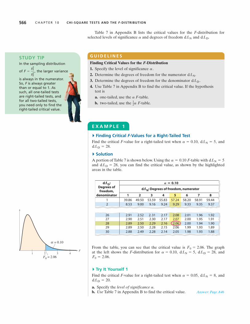
!Finding Critical F-Values for a Right-Tailed TestFind the critical F-value for a right-tailed test when and
!SolutionA portion of Table 7 is shown below. Using the F-table with and you can find the critical value, as shown by the highlightedareas in the table.
From the table, you can see that the critical value is The graph at the left shows the F-distribution for and
!Try It Yourself 1Find the critical F-value for a right-tailed test when and
a. Specify the level of significanceb. Use Table 7 in Appendix B to find the critical value. Answer: Page A46
a.
d.f.D = 20.d.f.N = 8,a = 0.05,
F0 = 2.06.d.f.D = 28,d.f.N = 5,a = 0.10,
F0 = 2.06.
# ! 0.10
26 2.91 2.52 2. 31 2.17 2.08 2.01 1.96 1.9227 2.90 2.51 2.30 2.17 2.07 2.00 1.95 1.9128 2.89 2.50 2.29 2.16 2.06 2.00 1.94 1.9029 2.89 2.50 2.28 2.15 2.06 1.99 1.93 1.8930 2.88 2.49 2.28 2.14 2.05 1.98 1.93 1.88
1 2 3 4 5 6 7 8 1 39.86 49.50 53.59 55.83 57.24 58.20 58.91 59.442 8.53 9.00 9.16 9.24 9.29 9.33 9.35 9.37
d.f.N: Degrees of freedom, numerator
d.f.D:Degrees of freedom,
denominator
d.f.D = 28,d.f.N = 5a = 0.10
d.f.D = 28.d.f.N = 5,a = 0.10,
Finding Critical Values for the F-Distribution1. Specify the level of significance 2. Determine the degrees of freedom for the numerator 3. Determine the degrees of freedom for the denominator 4. Use Table 7 in Appendix B to find the critical value. If the hypothesis
test isa. one-tailed, use the F-table.b. two-tailed, use the F-table.1
2a
a
d.f.D.d.f.N.
a .
G U I D E L I N E S
Table 7 in Appendix B lists the critical values for the F-distribution for selected levels of significance and degrees of freedom and d.f.D.d.f.Na
1 2 3 4 F
F0 = 2.06
α = 0.10
STUDY TIPIn the sampling distribution
of the larger variance
is always in the numerator. So, F is always greater than or equal to 1. As such, all one-tailed tests are right-tailed tests, and for all two-tailed tests, you need only to find the right-tailed critical value.
F =s21
s22,

S E C T I O N 1 0 . 3 COMPARING TWO VARIANCES 567
E X A M P L E 2
!Finding Critical F-Values for a Two-Tailed TestFind the critical F-value for a two-tailed test when and
!SolutionA portion of Table 7 is shown below. Using the
F-table with and you can find the critical value, as shownby the highlighted areas in the table.
From the table, the critical value is The graph shows the F-distribution for and
!Try It Yourself 2Find the critical F-value for a two-tailed test when and
a. Specify the level of significanceb. Use Table 7 in Appendix B with to find the critical value.
Answer: Page A46
12aa.
d.f.D = 5.d.f.N = 2,a = 0.01,
654321F
F0 = 5.05
α = 0.02512
F0 = 5.05.d.f.D = 8,d.f.N = 4,12a = 0.025,
F0 = 5.05.
# ! 0.025
1 2 3 4 5 6 7 81 647.8 799.5 864.2 899.6 921.8 937.1 948.2 956.72 38.51 39.00 39.17 39.25 39.30 39.33 39.36 39.373 17.44 16.04 15.44 15.10 14.88 14.73 14.62 14.544 12.22 10.65 9.98 9.60 9.36 9.20 9.07 8.985 10.01 8.43 7.76 7.39 7.15 6.98 6.85 6.766 8.81 7.26 6.60 6.23 5.99 5.82 5.70 5.607 8.07 6.54 5.89 5.52 5.29 5.12 4.99 4.908 7.57 6.06 5.42 5.05 4.82 4.65 4.53 4.439 7.21 5.71 5.08 4.72 4.48 4.32 4.20 4.10
d.f.N: Degrees of freedom, numerator
d.f.D:Degrees offreedom,
denominator
d.f.D = 8,d.f.N = 4,
12a = 1
210.052 = 0.025
d.f.D = 8.d.f.N = 4,a = 0.05,
When performing a two-tailed hypothesis test using the F-distribution, you needonly to find the right-tailed critical value. You must, however, remember to usethe F-table.1
2a
STUDY TIPWhen using Table 7 in Appendix Bto find a critical value, you willnotice that some of the values for
or are not included in the table. If or is exactly midway between two values in the table, then use the critical value midway between the corresponding critical values. In some cases, though, it is easier to use a technology tool to calculate the P-value,compare it to the level of significance, and then decide whether to reject the null hypothesis.
d.f.Dd.f.Nd.f.Dd.f.N

568 C H A P T E R 1 0 CHI-SQUARE TESTS AND THE F -DISTRIBUTION
" THE TWO-SAMPLE F-TEST FOR VARIANCESIn the remainder of this section, you will learn how to perform a two-sample F-test for comparing two population variances using a sample from eachpopulation. Such a test has three conditions that must be met.
1. The samples must be randomly selected.
2. The samples must be independent.
3. Each population must have a normal distribution.
If these requirements are met, you can use the F-test to compare the populationvariances and s2
2.s21
Using a Two-Sample F-Test to Compare and
IN WORDS IN SYMBOLS1. Identify the claim. State the null and State and
alternative hypotheses.
2. Specify the level of significance. Identify
3. Determine the degrees of freedom.
4. Determine the critical value. Use Table 7 inAppendix B.
5. Determine the rejection region.
6. Find the test statistic and sketchthe sampling distribution.
7. Make a decision to reject or fail to reject If F is in the rejectionthe null hypothesis. region, reject
Otherwise, fail toreject
8. Interpret the decision in the context ofthe original claim.
H0.
H0.
F =s21s22
d.f.D = n2 - 1d.f.N = n1 - 1
a.
Ha.H0
S22S2
1
G U I D E L I N E S
A two-sample F-test is used to compare two population variances and when a sample is randomly selected from each population. The populations must be independent and normally distributed.The test statistic is
where and represent the sample variances with The numeratorhas degrees of freedom and the denominator has
degrees of freedom, where is the size of the sample havingvariance and is the size of the sample having variance s22.n2s21
n1d.f.D = n2 - 1d.f.N = n1 - 1
s21 Ú s22.s22s21
F =s1
2
s22
s22s2
1
T W O - S A M P L E F - T E S T F O R VA R I A N C E S

S E C T I O N 1 0 . 3 COMPARING TWO VARIANCES 569
PICTURING THEWORLD
Does location have an effect onthe variance of real estate sellingprices? A random sample of selling prices (in thousands ofdollars) of condominiums sold in south Florida is shown in the table. The first columnrepresents the selling prices ofcondominiums in Miami, and thesecond column lists the sellingprices of condominiums in FortLauderdale. (Adapted from FloridaRealtors® and the University of FloridaBergstrom Center for Real Estate Studies)
Assuming each population of selling prices is normally distributed, is it possible to use a two-sample F-test to compare the population variances?
MiamiFort
Lauderdale
139.0 85.5
138.8 80.9
135.5 91.2
150.9 75.5
155.0 78.0
154.7 69.9
149.9 70.5
150.5 73.6
134.5 105.9
125.0 70.0
Normalsolution
Treatedsolution
n = 25 n = 20
s2 = 180 s2 = 56
E X A M P L E 3
!Performing a Two-Sample F-TestA restaurant manager is designing a system that is intended to decrease thevariance of the time customers wait before their meals are served. Under theold system, a random sample of 10 customers had a variance of 400. Under thenew system, a random sample of 21 customers had a variance of 256. At
is there enough evidence to convince the manager to switch to thenew system? Assume both populations are normally distributed.
!Solution Because and Therefore,and represent the sample and population variances for the old system,respectively. With the claim “the variance of the waiting times under the newsystem is less than the variance of the waiting times under the old system,” thenull and alternative hypotheses are
and (Claim)
Because the test is a right-tailed test with and the critical value is
So, the rejection region is With the F-test, the test statistic is
The graph shows the location of the rejection region and the test statistic. BecauseF is not in the rejection region, you should fail to reject the null hypothesis.
Interpretation There is not enough evidence at the 10% level of significanceto convince the manager to switch to the new system.
!Try It Yourself 3A medical researcher claims that a specially treated intravenous solutiondecreases the variance of the time required for nutrients to enter the bloodstream. Independent samples from each type of solution are randomlyselected, and the results are shown in the table at the left.At is thereenough evidence to support the researcher’s claim? Assume the populationsare normally distributed.
a. Identify the claim and state and b. Specify the level of significancec. Determine the degrees of freedom for the numerator and for the denominator.d. Determine the critical value and the rejection region.e. Use the F-test to find the test statistic F. Sketch a graph.f. Decide whether to reject the null hypothesis.g. Interpret the decision in the context of the original claim.
Answer: Page A46
a.Ha.H0
a = 0.01,
1 2 3 4 F
F0 = 1.96 F ≈ 1.56
α = 0.10
F =s21s22
= 400256
L 1.56.
F 7 1.96.F0 = 1.96.d.f.D = n2 - 1 = 21 - 1 = 20,10 - 1 = 9,
d.f.N = n1 - 1 =a = 0.10,
Ha: s21 7 s2
2 .H0: s21 … s2
2
s21
s21s22 = 256.s21 = 400,400 7 256,
a = 0.10,

570 C H A P T E R 1 0 CHI-SQUARE TESTS AND THE F -DISTRIBUTION
E X A M P L E 4
!Using Technology for a Two-Sample F-TestYou want to purchase stock in a company and are deciding between twodifferent stocks. Because a stock’s risk can be associated with the standarddeviation of its daily closing prices, you randomly select samples of the dailyclosing prices for each stock to obtain the results shown at the left. At
can you conclude that one of the two stocks is a riskier investment?Assume the stock closing prices are normally distributed.
!SolutionBecause and Therefore, and representthe sample and population variances for Stock B, respectively. With the claim “one of the two stocks is a riskier investment,” the null and alternativehypotheses are
and (Claim)
Because the test is a two-tailed test with and the critical value
is So, the rejection region is To perform a two-sample F-test using a TI-83/84 Plus, begin with the STATkeystroke. Choose the TESTS menu and select D:2–SampFTest. Then set upthe two-sample F-test as shown in the first screen below. Because you areentering the descriptive statistics, select the Stats input option. When enteringthe original data, select the Data input option. The other displays below showthe results of selecting Calculate or Draw.
The test statistic is in the rejection region, so you should reject thenull hypothesis.Interpretation There is enough evidence at the 5% level of significance tosupport the claim that one of the two stocks is a riskier investment.
!Try It Yourself 4A biologist claims that the pH levels of the soil in two geographic locationshave equal standard deviations. Independent samples from each location arerandomly selected, and the results are shown at the left. At is thereenough evidence to reject the biologist’s claim? Assume the pH levels are normally distributed.
a. Identify the claim and state and b. Specify the level of significancec. Determine the degrees of freedom for the numerator and for the denominator.d. Determine the critical value and the rejection region.e. Use a technology tool to find the test statistic F.f. Decide whether to reject the null hypothesis.g. Interpret the decision in the context of the original claim.
Answer: Page A46
a .Ha .H0
a = 0.01,
F L 2.652
F 7 2.09.F0 = 2.09.d.f.D = n2 - 1 = 30 - 1 = 29,n1 - 1 = 31 - 1 = 30,
d.f.N =12a = 1
210.052 = 0.025,
Ha: s21 Z s2
2 .H0: s21 = s2
2
s21s21s22 = 3.52.s21 = 5.72,5.72 7 3.52,
a = 0.05,
T I - 8 3 / 8 4 PLUS T I - 8 3 / 8 4 PLUS T I - 8 3 / 8 4 PLUS
Stock A Stock B
n2 = 30 n1 = 31
s2 = 3.5 s1 = 5.7
Location A Location B
n = 16 n = 22
s = 0.95 s = 0.78
STUDY TIPYou can also use a P-value to perform a two-sample F-test.For instance, in Example 4, note that the TI-83/84 Plus displays P .0102172459.Because P , you should reject the null hypothesis.
<A!
SC Report 48

S E C T I O N 1 0 . 3 COMPARING TWO VARIANCES 571
# BUILDING BASIC SKILLS AND VOCABULARY1. Explain how to find the critical value for an test.2. List five properties of the distribution.3. List the three conditions that must be met in order to use a two-sample test.4. Explain how to determine the values of and when performing a
two-sample test.
In Exercises 5–8, find the critical value for a right-tailed test using the indicatedlevel of significance and degrees of freedom and
5. 6.
7. 8.
In Exercises 9–12, find the critical F-value for a two-tailed test using the indicatedlevel of significance and degrees of freedom and
9. 10.
11. 12.
In Exercises 13–18, test the claim about the difference between two population variances and at the given level of significance using the given samplestatistics. Assume the sample statistics are from independent samples that arerandomly selected and each population has a normal distribution.
13. Claim: 14. Claim:Sample statistics: Sample statistics:
15. Claim: 16. Claim:Sample statistics: Sample statistics:
17. Claim: 18. Claim:Sample statistics: Sample statistics:
# USING AND INTERPRETING CONCEPTSComparing Two Variances In Exercises 19–26, (a) identify the claim andstate and (b) determine the critical value and the rejection region, (c) findthe test statistic F, (d) decide whether to reject or fail to reject the null hypothesis,and (e) interpret the decision in the context of the original claim. If convenient, use technology to solve the problem. In each exercise, assume the samples are independent and each population has a normal distribution.
19. Life of Appliances Company A claims that the variance of the life of itsappliances is less than the variance of the life of Company B’s appliances. Arandom sample of the lives of 20 of Company A’s appliances has a varianceof 2.6. A random sample of the lives of 25 of Company B’s appliances has avariance of 2.8. At can you support Company A’s claim? a = 0.05,
Ha,H0
n1 = 16; s22 = 39.3, n2 = 12n1 = 13; s22 = 2.5, n2 = 20s21 = 44.6,s21 = 9.8,
s21 7 s2
2; a = 0.05.s21 = s2
2; a = 0.01.
n1 = 31; s22 = 112, n2 = 28n1 = 11; s22 = 836, n2 = 10s21 = 245,s21 = 842,
s21 Z s2
2; a = 0.05.s21 … s2
2; a = 0.01.
n1 = 7; s22 = 297, n2 = 8n1 = 5; s22 = 765, n2 = 6s21 = 310,s21 = 773,
s21 = s2
2; a = 0.05.s21 7 s2
2; a = 0.10.
as22s2
1
a = 0.05, d.f.N = 27, d.f.D = 19a = 0.05, d.f.N = 60, d.f.D = 40
a = 0.10, d.f.N = 24, d.f.D = 28a = 0.01, d.f.N = 6, d.f.D = 7
d.f.D .d.f.Na
a = 0.025, d.f.N = 7, d.f.D = 3a = 0.10, d.f.N = 10, d.f.D = 15
a = 0.01, d.f.N = 2, d.f.D = 11a = 0.05, d.f.N = 9, d.f.D = 16
d.f.D .d.f.NaF-
F-d.f.Dd.f.N
F-F-
F-
10.3 EXERCISES

20. Fuel Consumption An automobile manufacturer claims that the variance ofthe fuel consumption for its hybrid vehicles is less than the variance of the fuelconsumption for the hybrid vehicles of a top competitor. A random sample ofthe fuel consumption of 19 of the manufacturer’s hybrids has a variance of 0.24.A random sample of the fuel consumption of 21 of its competitor’s hybrids hasa variance of 0.77. At can you support the manufacturer’s claim?(Adapted from GreenHybrid)
21. Home Theater Prices The table shows the prices (in dollars) for a randomsample of home theater systems. At can you conclude that the variances of the prices differ between the two companies? (Adapted from Best Buy)
22. Ice Cream and Calories The table shows the numbers of calories in aserving for a random sample of ice cream flavors for two brands. At
can you conclude that the variances of the numbers of caloriesdiffer between the two brands? (Source: Perry’s Ice Cream and Ben & Jerry’sHomemade, Inc.)
23. Science Assessment Tests In a recent interview, a state school administratorstated that the standard deviations of science assessment test scores foreighth grade students are the same in Districts 1 and 2. A random sample of12 test scores from District 1 has a standard deviation of 36.8 points, and arandom sample of 14 test scores from District 2 has a standard deviation of32.5 points. At can you reject the administrator’s claim? (Adaptedfrom National Center for Educational Statistics)
24. U.S. History Assessment Tests A school administrator reports that thestandard deviations of U.S. history assessment test scores for eighth gradestudents are the same in Districts 1 and 2.As proof, the administrator gives theresults of a study of test scores in each district. The study shows that a randomsample of 10 test scores from District 1 has a standard deviation of 33.9 points,and a random sample of 13 test scores from District 2 has a standard deviationof 30.2 points.At can you reject the administrator’s claim? (Adaptedfrom National Center for Educational Statistics)
25. Annual Salaries The annual salaries for a random sample of 16 actuariesworking in New York have a standard deviation of $14,900. The annualsalaries for a random sample of 17 actuaries working in California have astandard deviation of $9600.At can you conclude that the standarddeviation of the annual salaries for actuaries is greater in New York than inCalifornia? (Adapted from America’s Career InfoNet)
26. Annual Salaries An employment information service claims the standarddeviation of the annual salaries for public relations managers is greater inFlorida than in Louisiana. The annual salaries for a random sample of 28public relations managers in Florida have a standard deviation of $10,100.The annual salaries for a random sample of 24 public relations managers inLouisiana have a standard deviation of $6400. At can you supportthe service’s claim? (Adapted from America’s Career InfoNet)
In Exercises 27–30, use StatCrunch to test the claim about the differencebetween two population variances and at the given level of significance using the given sample statistics.Assume the sample statistics are from independentsamples that are randomly selected and each population has a normal distribution.
27. Claim: 28. Claim:Sample statistics: Sample statistics:
n1 = 24; s22 = 11.56, n2 = 20n1 = 15; s22 = 295.84, n2 = 18s21 = 31.36,s21 = 156.25,
s21 Z s2
2; a = 0.05.s21 = s2
2; a = 0.10.
as22s2
1
SC
a = 0.05,
a = 0.05,
a = 0.01,
a = 0.10,
a = 0.10,
a = 0.05,
a = 0.01,
572 C H A P T E R 1 0 CHI-SQUARE TESTS AND THE F -DISTRIBUTION
Company A Company B
250 350650 550285
450 400 350250 350 190550
TABLE FOR EXERCISE 21
Brand A Brand B
150 170 140160 140 130160 160 130180
270 250 300250 290 280240 310 240330
TABLE FOR EXERCISE 22
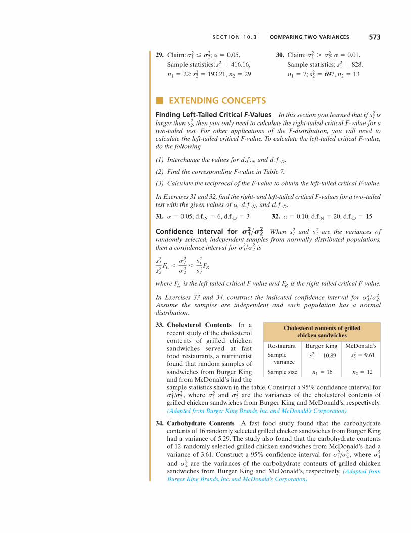
S E C T I O N 1 0 . 3 COMPARING TWO VARIANCES 573
29. Claim: 30. Claim:Sample statistics: Sample statistics:
# EXTENDING CONCEPTSFinding Left-Tailed Critical F-Values In this section you learned that if is larger than then you only need to calculate the right-tailed critical F-value for atwo-tailed test. For other applications of the F-distribution, you will need tocalculate the left-tailed critical F-value. To calculate the left-tailed critical F-value,do the following.
(1) Interchange the values for and
(2) Find the corresponding F-value in Table 7.
(3) Calculate the reciprocal of the F-value to obtain the left-tailed critical F-value.
In Exercises 31 and 32, find the right- and left-tailed critical F-values for a two-tailedtest with the given values of and
31. 32.
Confidence Interval for When and are the variances ofrandomly selected, independent samples from normally distributed populations,then a confidence interval for is
where is the left-tailed critical F-value and is the right-tailed critical F-value.
In Exercises 33 and 34, construct the indicated confidence interval for Assume the samples are independent and each population has a normaldistribution.
33. Cholesterol Contents In arecent study of the cholesterolcontents of grilled chickensandwiches served at fast food restaurants, a nutritionistfound that random samples of sandwiches from Burger Kingand from McDonald’s had thesample statistics shown in the table. Construct a 95% confidence interval for
where and are the variances of the cholesterol contents ofgrilled chicken sandwiches from Burger King and McDonald’s, respectively.(Adapted from Burger King Brands, Inc. and McDonald’s Corporation)
34. Carbohydrate Contents A fast food study found that the carbohydrate contents of 16 randomly selected grilled chicken sandwiches from Burger Kinghad a variance of 5.29. The study also found that the carbohydrate contents of 12 randomly selected grilled chicken sandwiches from McDonald’s had avariance of 3.61. Construct a 95% confidence interval for where and are the variances of the carbohydrate contents of grilled chicken sandwiches from Burger King and McDonald’s, respectively. (Adapted fromBurger King Brands, Inc. and McDonald’s Corporation)
s22
s21s2
1>s22 ,
s22s2
1s21>s2
2 ,
s21>s2
2.
FRFL
s21
s22
FL 6s2
1
s22
6s2
1
s22
FR
s21>s2
2
s22s2
1S21>S2
2
a = 0.10, d.f.N = 20, d.f.D = 15a = 0.05, d.f.N = 6, d.f.D = 3
d.f.D.d.f.N,a,
d.f.D.d.f.N
s22,
s21
n1 = 7; s22 = 697, n2 = 13n1 = 22; s22 = 193.21, n2 = 29s21 = 828,s21 = 416.16,
s21 7 s2
2; a = 0.01.s21 … s2
2; a = 0.05.
Cholesterol contents of grilled chicken sandwiches
Restaurant Burger King McDonald’s
Samplevariance
s12 = 10.89 s22 = 9.61
Sample size n1 = 16 n2 = 12

574 C H A P T E R 1 0 CHI-SQUARE TESTS AND THE F -DISTRIBUTION
" ONE-WAY ANOVASuppose a medical researcher is analyzing the effectiveness of three types of painrelievers and wants to determine whether there is a difference in the meanlengths of time it takes the three medications to provide relief. To determinewhether such a difference exists, the researcher can use the F-distributiontogether with a technique called analysis of variance. Because one independentvariable is being studied, the process is called one-way analysis of variance.
To begin a one-way analysis of variance test, you should first state the nulland alternative hypotheses. For a one-way ANOVA test, the null and alternativehypotheses are always similar to the following statements.
(All population means are equal.)
At least one mean is different from the others.
When you reject the null hypothesis in an ANOVA test, you can concludethat at least one of the means is different from the others. Without performingmore statistical tests, however, you cannot determine which of the means isdifferent.
In a one-way ANOVA test, the following conditions must be true.
1. Each sample must be randomly selected from a normal, or approximately normal, population.
2. The samples must be independent of each other.3. Each population must have the same variance.
The test statistic for a one-way ANOVA test is the ratio of two variances: thevariance between samples and the variance within samples.
1. The variance between samples measures the differences related to thetreatment given to each sample and is sometimes called the mean squarebetween.
2. The variance within samples measures the differences related to entrieswithin the same sample. This variance, sometimes called the mean square within, is usually due to sampling error.
MSW
MSB
Test statistic =Variance between samplesVariance within samples
Ha:
m1 = m2 = m3 = Á = mkH0:
One-Way ANOVA " Two-Way ANOVA
" How to use one-way analysisof variance to test claimsinvolving three or more means
" An introduction to two-wayanalysis of variance
10.4 Analysis of Variance
WHAT YOU SHOULD LEARN
One-way analysis of variance is a hypothesis-testing technique that is used tocompare the means of three or more populations. Analysis of variance is usually abbreviated as ANOVA.
D E F I N I T I O N

If there is little or no difference between the means, then will be approximately equal to and the test statistic will be approximately 1.Values of F close to 1 suggest that you should fail to reject the null hypothesis.However, if one of the means differs significantly from the others, will begreater than and the test statistic will be greater than 1. Values of Fsignificantly greater than 1 suggest that you should reject the null hypothesis. Assuch, all one-way ANOVA tests are right-tailed tests. That is, if the test statistic isgreater than the critical value, will be rejected.H0
MSWMSB
MSWMSB
Note that in Step 1, you are summing the values from just one sample. In Step 2,you are summing the values from all of the samples.
S E C T I O N 1 0 . 4 ANALYSIS OF VARIANCE 575
STUDY TIPThe notations and represent the sample size, mean, and variance of the ith sample, respectively.
is sometimes called the grand mean.x
s2ixi ,ni , Finding the Test Statistic for a One-Way ANOVA Test
IN WORDS IN SYMBOLS
1. Find the mean and variance of each sample.
2. Find the mean of all entries inall samples (the grand mean).
3. Find the sum of squares betweenthe samples.
4. Find the sum of squares withinthe samples.
5. Find the variance between thesamples.
6. Find the variance within thesamples.
7. Find the test statistic. F =MSBMSW
MSW =SSWd.f.D
=g1ni - 12s2iN - k
MSB =SSBd.f.N
=gni Axi - x B2k - 1
SSW = g1ni - 12si2SSB = gni Axi - x B2x = gx
N
s2 =g1x - x22n - 1
x = gxn
,
G U I D E L I N E S
If the conditions for a one-way analysis of variance test are satisfied, then thesampling distribution for the test is approximated by the F-distribution. Thetest statistic is
The degrees of freedom for the F-test are
and
where k is the number of samples and N is the sum of the sample sizes.
d.f.D = N - k
d.f.N = k - 1
F =MSBMSW
.
O N E - W AY A N A LY S I S O F VA R I A N C E T E S T

The notation represents the sum of squares between the samples.
The notation represents the sum of squares within the samples.
= g1ni - 12s2iSSW = 1n1 - 12s21 + 1n2 - 12s22 + Á + 1nk - 12s2kSSW
= gni Axi - x B2SSB = n1 Ax1 - x B2 + n2 Ax2 - x B2 + Á + nk Axk - x B2SSB
Tables are a convenient way to summarize the results of a one-way analysisof variance test. ANOVA summary tables are set up as shown below.
576 C H A P T E R 1 0 CHI-SQUARE TESTS AND THE F -DISTRIBUTION
Performing a One-Way Analysis of Variance Test
IN WORDS IN SYMBOLS1. Identify the claim. State the null and State and
alternative hypotheses.
2. Specify the level of significance. Identify
3. Determine the degrees of freedom.
4. Determine the critical value. Use Table 7 inAppendix B.
5. Determine the rejection region.
6. Find the test statistic and sketchthe sampling distribution.
7. Make a decision to reject or fail to reject If F is in the rejec-the null hypothesis. tion region, reject
Otherwise, failto reject
8. Interpret the decision in the context ofthe original claim.
H0.H0.
F =MSBMSW
d.f.D = N - kd.f.N = k - 1
a.
Ha.H0
G U I D E L I N E S
VariationSum ofsquares
Degrees offreedom
Meansquares F
Between SSB d.f.N MSB =SSBd.f.N
MSBMSW
Within SSW d.f.D MSW =SSWd.f.D
ANOVA Summary Table

S E C T I O N 1 0 . 4 ANALYSIS OF VARIANCE 577
E X A M P L E 1
!Performing a One-Way ANOVA TestA medical researcher wants to determine whether there is a difference in themean lengths of time it takes three types of pain relievers to provide relieffrom headache pain. Several headache sufferers are randomly selected andgiven one of the three medications. Each headache sufferer records the time (inminutes) it takes the medication to begin working.The results are shown in thetable. At can you conclude that at least one mean time is differentfrom the others? Assume that each population of relief times is normally distributed and that the population variances are equal.
!Solution The null and alternative hypotheses are as follows.
At least one mean is different from the others. (Claim)
Because there are samples, The sum of thesample sizes is So,
Using and the critical value isTo find the test statistic, first calculate and
Using and the test statistic is
F =MSBMSW
L 10.96167.3
L 1.50.
MSW = 7.3,MSB L 10.9616
= 7310
= 7.3=14 - 12162 + 15 - 1218.52 + 14 - 12172
13 - 3
MSW =SSWd.f.D
=g1ni - 12s2iN - k
= 21.92322
= 10.9616
L4114 - 15.9222 + 5117 - 15.9222 + 4116.5 - 15.9222
3 - 1
MSB =SSBd.f.N
=gni Axi - x B2k - 1
x = gxN
= 56 + 85 + 6613
L 15.92
MSW.MSB,x,F0 = 7.56.a = 0.01,d.f.D = 10,d.f.N = 2,13 - 3 = 10.
d.f.D = N - k =N = n1 + n2 + n3 = 4 + 5 + 4 = 13.d.f.N = k - 1 = 3 - 1 = 2.k = 3
Ha:
m1 = m2 = m3H0:
a = 0.01,
Medication 1 Medication 2 Medication 3
12 16 14
15 14 17
17 21 20
12 15 15
19
n1 = 4 n2 = 5 n3 = 4
x1 = 564 = 14 x2 = 85
5 = 17 x3 = 664 = 16.5
s21 = 6 s22 = 8.5 s23 = 7

578 C H A P T E R 1 0 CHI-SQUARE TESTS AND THE F -DISTRIBUTION
PICTURING THEWORLD
A researcher wants to determinewhether there is a difference inthe mean lengths of time wastedat work for people in California,Georgia, and Pennsylvania.Several people from each statewho work 8-hour days are randomly selected and they areasked how much time (in hours)they waste at work each day. The results are shown in thetable. (Adapted from America Online andSalary.com)
At 0.10, can the researcherconclude that there is a difference in the mean lengths of time wasted at work amongthe states? Assume that eachpopulation is normally distributed and that the population variances are equal.
A !
CA GA PA
2 2 1.75
1.75 2.5 3
2.5 1.25 2.75
3 2.25 2
2.75 1.5 3
3.25 3 2.5
1.25 2.75 2.75
2 2.25 3.25
2.5 2 3
1.75 1 2.75
1.5 2.25
2.25
The graph shows the location of therejection region and the test statistic.Because F is not in the rejectionregion, you should fail to reject the nullhypothesis.Interpretation There is not enoughevidence at the 1% level of significanceto conclude that there is a difference inthe mean length of time it takes thethree pain relievers to provide relieffrom headache pain.
The ANOVA summary table for Example 1 is shown below.
!Try It Yourself 1A sales analyst wants to determine whether there is a difference in the meanmonthly sales of a company’s four sales regions. Several salespersons fromeach region are randomly selected and they provide their sales amounts (inthousands of dollars) for the previous month. The results are shown in thetable. At can the analyst conclude that there is a difference in themean monthly sales among the sales regions? Assume that each population ofsales is normally distributed and that the population variances are equal.
a. Identify the claim and state and b. Specify the level of significancec. Determine the degrees of freedom for the numerator and for the denominator.d. Determine the critical value and the rejection region.e. Find the test statistic F. Sketch a graph.f. Decide whether to reject the null hypothesis.g. Interpret the decision in the context of the original claim.
Answer: Page A46
a .Ha .H0
a = 0.05,
VariationSum ofsquares
Degrees offreedom
Meansquares F
Between
Within
21.9232
73
2
10
10.9616
7.3
1.50
North East South West
34 47 40 21
28 36 30 30
18 30 41 24
24 38 29 37
44 23
n1 = 4 n2 = 5 n3 = 4 n4 = 5
x1 = 26 x2 = 39 x3 = 35 x4 = 27
s21 L 45.33 s22 = 45 s2
3 L 40.67 s42 = 42.5
2 4 6 8 F
F0 = 7.56 F ≈ 1.50
α = 0.01
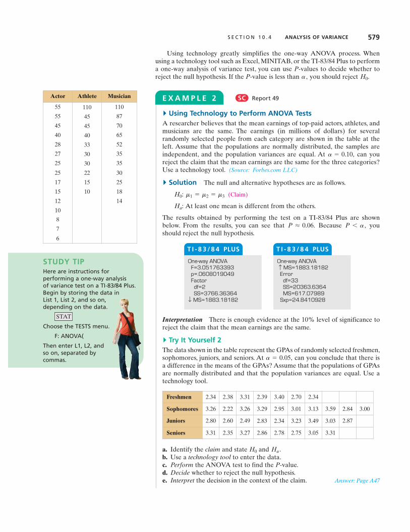
Using technology greatly simplifies the one-way ANOVA process. Whenusing a technology tool such as Excel, MINITAB, or the TI-83/84 Plus to performa one-way analysis of variance test, you can use P-values to decide whether toreject the null hypothesis. If the P-value is less than you should reject H0.a ,
S E C T I O N 1 0 . 4 ANALYSIS OF VARIANCE 579
Actor Athlete Musician
55 110 110
55 45 87
45 45 70
40 40 65
28 33 52
27 30 35
25 30 35
25 22 30
17 15 25
15 10 18
12 14
10
8
7
6
E X A M P L E 2
!Using Technology to Perform ANOVA TestsA researcher believes that the mean earnings of top-paid actors, athletes, andmusicians are the same. The earnings (in millions of dollars) for several randomly selected people from each category are shown in the table at the left. Assume that the populations are normally distributed, the samples are independent, and the population variances are equal. At can youreject the claim that the mean earnings are the same for the three categories?Use a technology tool. (Source: Forbes.com LLC)
!Solution The null and alternative hypotheses are as follows.
(Claim)
At least one mean is different from the others.
The results obtained by performing the test on a TI-83/84 Plus are shownbelow. From the results, you can see that Because youshould reject the null hypothesis.
Interpretation There is enough evidence at the 10% level of significance toreject the claim that the mean earnings are the same.
!Try It Yourself 2The data shown in the table represent the GPAs of randomly selected freshmen,sophomores, juniors, and seniors. At can you conclude that there isa difference in the means of the GPAs? Assume that the populations of GPAsare normally distributed and that the population variances are equal. Use atechnology tool.
a. Identify the claim and state and b. Use a technology tool to enter the data.c. Perform the ANOVA test to find the P-value.d. Decide whether to reject the null hypothesis.e. Interpret the decision in the context of the claim. Answer: Page A47
Ha .H0
a = 0.05,
P 6 a ,P L 0.06.
Ha:
m1 = m2 = m3H0:
a = 0.10,
STUDY TIPHere are instructions for performing a one-way analysis of variance test on a TI-83/84 Plus. Begin by storing the data in List 1, List 2, and so on, depending on the data.
Choose the TESTS menu.
F: ANOVA(
Then enter L1, L2, and so on, separated by commas.
STAT
T I - 8 3 / 8 4 PLUS
One-way ANOVAF=3.051763393p=.0608019049Factor
df=2SS=3766.36364
↓ MS=1883.18182
T I - 8 3 / 8 4 PLUS
One-way ANOVAMS=1883.18182
Errordf=33SS=20363.6364MS=617.07989
Sxp=24.8410928
↓
Freshmen 2.34 2.38 3.31 2.39 3.40 2.70 2.34
Sophomores 3.26 2.22 3.26 3.29 2.95 3.01 3.13 3.59 2.84 3.00
Juniors 2.80 2.60 2.49 2.83 2.34 3.23 3.49 3.03 2.87
Seniors 3.31 2.35 3.27 2.86 2.78 2.75 3.05 3.31
SC Report 49
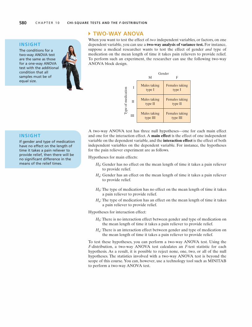
" TWO-WAY ANOVAWhen you want to test the effect of two independent variables, or factors, on onedependent variable, you can use a two-way analysis of variance test. For instance,suppose a medical researcher wants to test the effect of gender and type of medication on the mean length of time it takes pain relievers to provide relief.To perform such an experiment, the researcher can use the following two-wayANOVA block design.
A two-way ANOVA test has three null hypotheses—one for each main effectand one for the interaction effect. A main effect is the effect of one independentvariable on the dependent variable, and the interaction effect is the effect of bothindependent variables on the dependent variable. For instance, the hypothesesfor the pain reliever experiment are as follows.
Hypotheses for main effects:
Gender has no effect on the mean length of time it takes a pain relieverto provide relief.Gender has an effect on the mean length of time it takes a pain relieverto provide relief.
The type of medication has no effect on the mean length of time it takesa pain reliever to provide relief.The type of medication has an effect on the mean length of time it takesa pain reliever to provide relief.
Hypotheses for interaction effect:
There is no interaction effect between gender and type of medication onthe mean length of time it takes a pain reliever to provide relief.There is an interaction effect between gender and type of medication onthe mean length of time it takes a pain reliever to provide relief.
To test these hypotheses, you can perform a two-way ANOVA test. Using the F-distribution, a two-way ANOVA test calculates an F-test statistic for eachhypothesis. As a result, it is possible to reject none, one, two, or all of the nullhypotheses. The statistics involved with a two-way ANOVA test is beyond thescope of this course. You can, however, use a technology tool such as MINITABto perform a two-way ANOVA test.
Ha:
H0:
Ha:
H0:
Ha:
H0:
Males takingtype I
Males takingtype II
Males takingtype III
I
II
III
Females takingtype I
M F
Females takingtype II
Females takingtype III
Type
of m
edic
atio
n
Gender
580 C H A P T E R 1 0 CHI-SQUARE TESTS AND THE F -DISTRIBUTION
INSIGHTThe conditions for a two-way ANOVA test are the same as those for a one-way ANOVA test with the additional condition that all samples must be of equal size.
INSIGHTIf gender and type of medicationhave no effect on the length oftime it takes a pain reliever toprovide relief, then there will beno significant difference in themeans of the relief times.

S E C T I O N 1 0 . 4 ANALYSIS OF VARIANCE 581
# BUILDING BASIC SKILLS AND VOCABULARY1. State the null and alternative hypotheses for a one-way ANOVA test.
2. What conditions are necessary in order to use a one-way ANOVA test?
3. Describe the difference between the variance between samples and thevariance within samples
4. Describe the hypotheses for a two-way ANOVA test.
# USING AND INTERPRETING CONCEPTSPerforming a One-Way ANOVA Test In Exercises 5–14, (a) identify theclaim and state and (b) find the critical value and identify the rejectionregion, (c) find the test statistic F, (d) decide whether to reject or fail to reject the null hypothesis, and (e) interpret the decision in the context of the originalclaim. If convenient, use technology to solve the problem. In each exercise, assumethat each population is normally distributed and that the population variances are equal.
5. Toothpaste The table showsthe cost per ounce (in dollars)for a random sample oftoothpastes exhibiting verygood stain removal, goodstain removal, and fair stainremoval. At canyou conclude that the meancosts per ounce are different?(Source: Consumer Reports)
6. Automobile Batteries The prices (in dollars) of 17 randomly selected automobile batteries are shown in the table. The prices are classified according to battery type. At is there enough evidence to concludethat at least one of the mean battery prices is different from the others?(Source: Consumer Reports)
Group size 35 90 90 75 105 65
Group size 65 100 75 105 100 100 75
Group size 24/24F 115 75 75 90 110 90
a = 0.05,
a = 0.05,
Ha,H0
MSW.MSB
10.4 EXERCISES
Very goodstain removal
Good stainremoval
Fair stainremoval
0.47 0.60 0.34
0.49 0.64 0.46
0.33 1.05 1.31
1.52 2.73 0.44
0.64 0.58 0.600.36 0.75
0.41 0.22
0.37 0.33
0.48 0.42
0.50 0.46
0.51 0.98
0.35 1.16

7. Government Salaries The table shows the salaries (in thousands of dollars) of randomly selected individuals from the federal, state, and locallevels of government. At can you conclude that at least onemean salary is different? (Adapted from Bureau of Labor Statistics)
8. Late Night Hosts The table shows the ages (in years) of randomlyselected viewers for several late night hosts.At can you concludethat at least one mean age is different? (Adapted from The New York Times)
9. Cost Per Mile The table shows the cost per mile (in cents) for a randomsample of automobiles.At can you conclude that at least one meancost per mile is different? (Adapted from American Automobile Association)
Small sedan Medium sedan Large sedan 4WD SUV Minivan
40 62 59 84 63
38 44 68 63 73
46 58 78 72 56
51 54 70 75 48
43 59 75 67
47 67
a = 0.01,
JimmyFallon
CraigFerguson
JimmyKimmel
JayLeno
DavidLetterman
19 22 18 41 27
28 27 21 43 34
37 32 33 44 41
43 37 42 47 43
48 45 48 49 48
48 53 57 51 54
53 55 59 59 57
54 62 61 61 59
54 64 62 62 60
57 67 64 64 63
62 68 68 65 69
67 70 68 67 71
79 72 75 74 73
a = 0.05,
Federal State Local
63.7 50.6 47.1
56.4 34.7 36.6
67.8 51.7 40.9
75.6 52.2 39.3
74.9 54.4 49.9
79.0 59.5 44.0
49.6 37.6 58.6
64.5 48.1 39.1
74.2 51.3 35.5
57.9 45.1 31.7
a = 0.01,
582 C H A P T E R 1 0 CHI-SQUARE TESTS AND THE F -DISTRIBUTION

S E C T I O N 1 0 . 4 ANALYSIS OF VARIANCE 583
10. Well-Being Index The well-beingindex is a way to measure howpeople are faring physically,emotionally, socially, and professionally, as well as to ratethe overall quality of their livesand their outlooks for thefuture. The table shows thewell-being index scores for arandom sample of states fromfour regions of the UnitedStates. At can youreject the claim that the meanscore is the same for allregions? (Adapted from Gallupand Healthways)
11. Days Spent at the Hospital In a recent study, a health insurance company investigated the number of days patients spent at the hospital.In part of the study, the company randomly selected patients from various parts of the United States and recorded the number of dayseach patient spent at the hospital. The results of the study are shown inthe table. At can the company reject the claim that the meannumber of days patients spend at the hospital is the same for all fourregions? (Adapted from National Center for Health Statistics)
12. Personal Income The table shows the salaries of randomly selectedindividuals from six large metropolitan areas. At can you conclude that the mean salary is different in at least one of the areas?(Adapted from U.S. Bureau of Economic Analysis)
Chicago Dallas Miami Denver San Diego Seattle
41,950 34,315 43,500 41,400 46,000 56,135
36,100 31,500 47,350 42,580 43,100 46,500
45,200 38,000 34,700 46,600 41,550 44,400
51,400 49,495 46,500 49,900 52,300 51,000
50,920 38,700 39,050 53,175 39,400 55,875
40,500 51,050 42,900 44,000
45,060 47,700
a = 0.05,
Northeast Midwest South West
6 6 3 3
4 6 5 4
7 7 6 6
2 3 6 4
3 5 3 6
4 4 7 6
6 4 4 5
8 3 2
9 2
a = 0.01,
a = 0.10,
Northeast Midwest South West
66.9 67.3 67.0 70.2
67.4 67.6 66.2 68.3
65.0 67.8 66.1 67.3
65.4 67.2 66.8 68.3
66.7 66.5 64.8 66.4
64.2 64.9 64.9 67.3
63.6 65.1 63.8
63.9 64.2 65.3
63.9 66.064.0
60.5

13. Energy Consumption The table shows the energy consumed (in millions of Btu) in one year for a random sample of households fromfour regions of the United States. At can you conclude thatthe mean energy consumption of at least one region is different fromthe others? (Adapted from U.S. Energy Information Administration)
14. Amount Spent on Energy The table shows the amount spent (indollars) on energy in one year for a random sample of households fromfour regions of the United States. At can you reject the claimthat the mean amounts spent are equal for all regions? (Adapted fromU.S. Energy Information Administration)
In Exercises 15 and 16, use StatCrunch to perform a one-way ANOVA test.Decide whether to reject the null hypothesis. Then, interpret the decision in the context of the original claim.
15. Sports Team Involvement The table shows the number of female studentswho played on a sports team in grades 9 through 12 for a random sample of 8 high schools in a state. At can you reject the claim that themean numbers of female students who played on a sports team are equal for all grades?
Grade 9 82 91 53 133 64 112 63 77
Grade 10 77 87 58 125 51 106 58 72
Grade 11 86 81 46 115 56 87 62 80
Grade 12 65 77 42 102 49 84 65 82
a = 0.01,
SC
Northeast Midwest South West
1456 1940 1457 1168
3025 1570 2202 1927
2029 1972 1883 989
1735 1924 1310 2022
1956 1820 1876 1330
3078 2144 1578 1184
3023 1319 1980 1819
1709 1655
3425 1730
1684
a = 0.05,
Northeast Midwest South West
101.5 56.7 68.8 31.0
109.5 174.8 92.8 46.2
153.6 61.6 56.5 127.7
129.0 79.3 96.6 61.4
160.3 160.9 57.0 108.4
114.6 179.9 51.3 69.8
85.2 98.6 63.2 44.5
173.0 132.1 50.6 124.8
73.6 89.5 182.0 98.6
155.5 58.3
61.9
a = 0.10,
584 C H A P T E R 1 0 CHI-SQUARE TESTS AND THE F -DISTRIBUTION

S E C T I O N 1 0 . 4 ANALYSIS OF VARIANCE 585
16. Housing Prices The table shows the sale prices (in thousands of dollars) of randomly selected one-family houses in three cities. At can youconclude that at least one mean sale price is different? (Adapted from NationalAssociation of Realtors)
# EXTENDING CONCEPTSUsing Technology to Perform a Two-Way ANOVA Test In Exercises17–20, use a technology tool and the given block design to perform a two-wayANOVA test. Use Interpret the results.
17. Advertising A study was conducted in which a random sample of 20adults was asked to rate the effectiveness of advertisements. Each adultrated a radio or television advertisement that lasted 30 or 60 seconds.The block design shows these ratings (on a scale of 1 to 5, with 5 beingextremely effective).
18. Vehicle Sales The owner of a car dealership wants to determine if thegender of a salesperson and the type of vehicle sold affect the number ofvehicles sold in a month. The block design shows the number of vehicles,listed by type, sold in a month by a random sample of eight salespeople.
Male 6, 5, 4, 5 2, 2, 1, 3 4, 3, 4, 2
5, 7, 8, 7 1, 0, 1, 2 4, 2, 0, 1Female
Car Truck Van/SUV
Gen
der
Type of vehicle
30 sec 2, 3, 5, 1, 3 3, 5, 4, 1, 2
60 sec 2, 5, 3, 4, 41, 4, 2, 2, 5
Radio Television
Len
gth
of a
d
Advertising medium
a = 0.10.
Gainesville Orlando Tampa
179.0 253.9 229.9
151.5 211.1 114.9
196.6 195.3 210.2
192.3 197.5 202.7
254.7 217.9 149.1
212.4 244.8 166.0
92.8 263.2 133.3
210.6 154.7 213.4
180.5 173.9 104.7
226.0 183.3 215.4
179.0
a = 0.10,
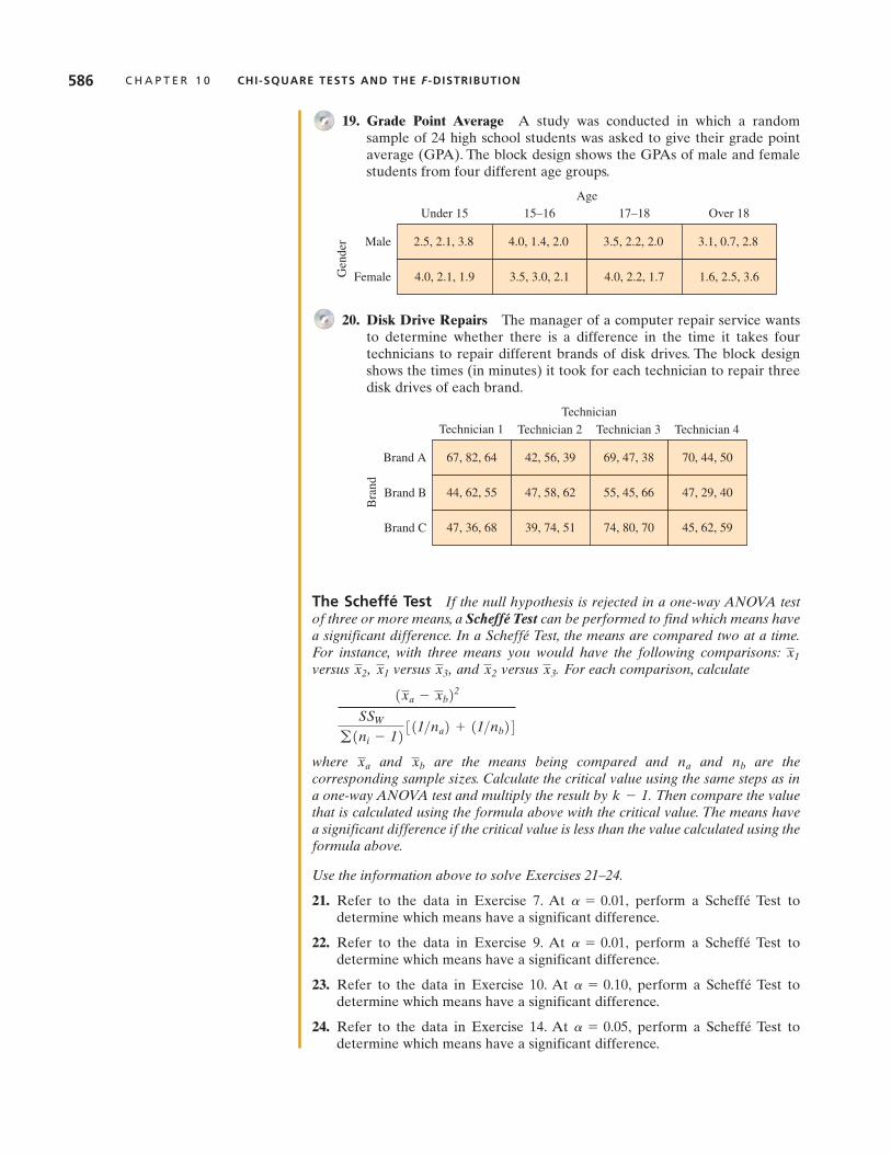
19. Grade Point Average A study was conducted in which a random sample of 24 high school students was asked to give their grade pointaverage (GPA). The block design shows the GPAs of male and femalestudents from four different age groups.
20. Disk Drive Repairs The manager of a computer repair service wantsto determine whether there is a difference in the time it takes four technicians to repair different brands of disk drives. The block designshows the times (in minutes) it took for each technician to repair threedisk drives of each brand.
The Scheffé Test If the null hypothesis is rejected in a one-way ANOVA testof three or more means, a Scheffé Test can be performed to find which means havea significant difference. In a Scheffé Test, the means are compared two at a time.For instance, with three means you would have the following comparisons:versus versus and versus For each comparison, calculate
where and are the means being compared and and are thecorresponding sample sizes. Calculate the critical value using the same steps as ina one-way ANOVA test and multiply the result by Then compare the valuethat is calculated using the formula above with the critical value. The means havea significant difference if the critical value is less than the value calculated using theformula above.
Use the information above to solve Exercises 21–24.
21. Refer to the data in Exercise 7. At perform a Scheffé Test to determine which means have a significant difference.
22. Refer to the data in Exercise 9. At perform a Scheffé Test to determine which means have a significant difference.
23. Refer to the data in Exercise 10. At perform a Scheffé Test todetermine which means have a significant difference.
24. Refer to the data in Exercise 14. At perform a Scheffé Test todetermine which means have a significant difference.
a = 0.05,
a = 0.10,
a = 0.01,
a = 0.01,
k - 1.
nbnaxbxa
1xa - xb22SSWg1ni - 12 311>na2 + 11>nb24
x3.x2x3,x1x2,x1
Brand A 67, 82, 64 42, 56, 39 69, 47, 38
44, 62, 55 47, 58, 62 55, 45, 66
70, 44, 50
47, 29, 40Brand B
47, 36, 68 39, 74, 51 74, 80, 70 45, 62, 59Brand C
Technician 1 Technician 2 Technician 3 Technician 4
Bra
nd
Technician
Male 2.5, 2.1, 3.8
Female 4.0, 2.1, 1.9
Under 15
4.0, 1.4, 2.0
3.5, 3.0, 2.1
15–16 17–18 Over 18
3.5, 2.2, 2.0
4.0, 2.2, 1.7
3.1, 0.7, 2.8
1.6, 2.5, 3.6Gen
der
Age
586 C H A P T E R 1 0 CHI-SQUARE TESTS AND THE F -DISTRIBUTION

UsesOne-Way Analysis of Variance (ANOVA) ANOVA can help you makeimportant decisions about the allocation of resources. For instance, supposeyou work for a large manufacturing company and part of your responsibilityis to determine the distribution of the company’s sales throughout the world anddecide where to focus the company’s efforts. Because wrong decisions will costyour company money, you want to make sure that you make the right decisions.
AbusesPreconceived Notions There are several ways that the tests presented in this chapter can be abused. For instance, it is easy to allow preconceivednotions to affect the results of a chi-square goodness-of-fit test and a test forindependence.When testing to see whether a distribution has changed, do not letthe existing distribution “cloud” the study results. Similarly, when determiningwhether two variables are independent, do not let your intuition “get in theway.” As with any hypothesis test, you must properly gather appropriate dataand perform the corresponding test before you can reach a logical conclusion.
Incorrect Interpretation of Rejection of Null Hypothesis It is important toremember that when you reject the null hypothesis of an ANOVA test, you aresimply stating that you have enough evidence to determine that at least one ofthe population means is different from the others.You are not finding them allto be different. One way to further test which of the population means differsfrom the others is explained in Extending Concepts in Section 10.4 Exercises.
# EXERCISES1. Preconceived Notions ANOVA depends on having independent variables.
Describe an abuse that might occur by having dependent variables. Thendescribe how the abuse could be avoided.
2. Incorrect Interpretation of Rejection of Null Hypothesis Find an example of the use of ANOVA. In that use, describe what would be meantby “rejection of the null hypothesis.” How should rejection of the nullhypothesis be correctly interpreted?
USES AND ABUSESUSES AND ABUSES 587
Statistics in the Real World

Section 10.1
! How to use the chi-square distribution to test whether a frequency distribution fits a claimed distribution
x2 = g 1O - E22E
1–3 1–4
Section 10.2
! How to use a contingency table to find expected frequencies
Er, c =1Sum of row r2 * 1Sum of column c2
Sample size
1 5–8
! How to use a chi-square distribution to test whether two variables are independent
2, 3 5–8
Section 10.3
! How to interpret the F-distribution and use an F-table to find critical values
F =s21s22
1, 2 9–16
! How to perform a two-sample F-test to compare two variances 3, 4 17–22
Section 10.4
! How to use one-way analysis of variance to test claims involving three or more means
F =MSBMSW
1, 2 23, 24
588 C H A P T E R 1 0 CHI-SQUARE TESTS AND THE F -DISTRIBUTION
10 CHAPTER SUMMARY
EXAMPLE(S)REVIEW
EXERCISESWhat did you learn?

REVIEW EXERCISES 589
# SECTION 10.1In Exercises 1–4, (a) identify the claimed distribution and state and (b) findthe critical value and identify the rejection region, (c) find the chi-square test statistic,(d) decide whether to reject or fail to reject the null hypothesis, and (e) interpret thedecision in the context of the original claim.
1. Results from a previous survey asking parents how much they give for anallowance are shown in the pie chart. To determine whether the distributionhas changed, you randomly select 1103 parents and ask them how much theygive for an allowance. The results are shown in the table. At can you conclude that there has been a change in the claimed or expected distribution? (Adapted from Echo Research)
2. Results from a survey 10 years ago asking people how long their office visitswith a physician were are shown in the pie chart. To determine whether this distribution has changed, a research organization randomly selects 350 people and asks them how long their office visits with a physician were.The results are shown in the table. At can you conclude that therehas been a change in the claimed or expected distribution? (Adapted fromNational Center for Health Statistics)
3. Results from a previous survey askinggolf students what they need the most help with in golf are shown in thepie chart. To determine whether thedistribution is the same, a golf instruc-tor randomly selects 435 golf studentsand asks them what they need themost help with in golf. The results areshown in the table. At arethe distributions the same? (Adaptedfrom PGA of America)
a = 0.05,
Survey results
Minutes Frequency, f
1–5 9
6–10 62
11–15 126
16–30 129
31–60 23
61 and over 1
1–54%
61 and over1%
31–606%
16–3031%
6–1024%
11–1534%
a = 0.01,
Survey results
Response Frequency, f
Less than $10 353
$10 to $20 167
More than $21 94
Don’t give one/other 489
a = 0.10,
Ha,H0
10 REVIEW EXERCISES
Don’t giveone/other
46%
Less than $1029% $10 to $20
16%
More than $219%
Drivershots9%
Short-game shots65%
Approach and swing22%
Putting4%
FIGURE FOR EXERCISE 1
FIGURE FOR EXERCISE 3
Survey results
Response Frequency, f
Short-game shots 276
Approach and swing 99
Driver shots 42
Putting 18
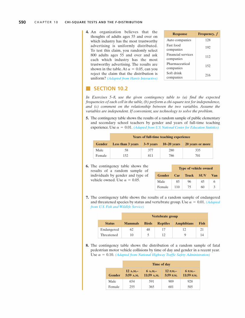
590 C H A P T E R 1 0 CHI-SQUARE TESTS AND THE F -DISTRIBUTION
4. An organization believes that thethoughts of adults ages 55 and over onwhich industry has the most trustworthyadvertising is uniformly distributed.To test this claim, you randomly select800 adults ages 55 and over and askeach which industry has the most trustworthy advertising. The results areshown in the table. At can youreject the claim that the distribution isuniform? (Adapted from Harris Interactive)
# SECTION 10.2In Exercises 5–8, use the given contingency table to (a) find the expectedfrequencies of each cell in the table, (b) perform a chi-square test for independence,and (c) comment on the relationship between the two variables. Assume thevariables are independent. If convenient, use technology to solve the problem.
5. The contingency table shows the results of a random sample of public elementaryand secondary school teachers by gender and years of full-time teaching experience. Use (Adapted from U.S. National Center for Education Statistics)
6. The contingency table shows theresults of a random sample of individuals by gender and type ofvehicle owned. Use
7. The contingency table shows the results of a random sample of endangeredand threatened species by status and vertebrate group. Use (Adaptedfrom U.S. Fish and Wildlife Service)
8. The contingency table shows the distribution of a random sample of fatalpedestrian motor vehicle collisions by time of day and gender in a recent year.Use (Adapted from National Highway Traffic Safety Administration)a = 0.10.
a = 0.01.
a = 0.05.
a = 0.01.
a = 0.05,
Response Frequency, f
Auto companies 128Fast food companies 192
Financial services companies 112
Pharmaceutical companies 152
Soft drink companies 216
Type of vehicle owned
Gender Car Truck SUV Van
Male 85 96 45 6
Female 110 75 60 3
Vertebrate group
Status Mammals Birds Reptiles Amphibians Fish
Endangered 62 48 17 12 21
Threatened 10 5 12 9 14
Time of day
Gender12 A.M.–5:59 A.M.
6 A.M.–11:59 A.M.
12 P.M.–5:59 P.M.
6 P.M.–11:59 P.M.
Male 654 591 909 928
Female 255 365 601 505
Years of full-time teaching experience
Gender Less than 3 years 3–9 years 10–20 years 20 years or more
Male 58 377 280 335
Female 152 811 786 701

REVIEW EXERCISES 591
# SECTION 10.3In Exercises 9–12, find the critical F-value for a right-tailed test using the indicatedlevel of significance and degrees of freedom and
9. 10.
11. 12.
In Exercises 13–16, find the critical F-value for a two-tailed test using the indicatedlevel of significance and degrees of freedom and
13. 14.
15. 16.
In Exercises 17 and 18, test the claim about the difference between two populationvariances and at the indicated level of significance using the given samplestatistics. Assume the sample statistics are from independent samples that arerandomly selected and each population has a normal distribution.
17. Claim: Sample statistics:
18. Claim: Sample statistics:
In Exercises 19–22, test the claim about two population variances at the indicatedlevel of significance Interpret the results in the context of the claim. If convenient, use technology to solve the problem. In each exercise, assume the samples are independent and each population has a normal distribution.
19. An agricultural analyst is comparing the wheat production in Oklahomacounties. The analyst claims that the variation in wheat production is greaterin Garfield County than in Kay County. A random sample of 21 GarfieldCounty farms yields a standard deviation of 0.76 bushel per acre. A randomsample of 16 Kay County farms is found to have a standard deviation of 0.58 bushel per acre. Test the analyst’s claim at (Adapted fromEnvironmental Verification and Analysis Center—University of Oklahoma)
20. A travel consultant indicates that the standard deviations of hotel room ratesfor San Francisco, CA and Sacramento, CA are the same. A random sampleof 36 hotel room rates in San Francisco has a standard deviation of $75 anda random sample of 31 hotel room rates in Sacramento has a standard deviation of $44. At can you reject the travel consultant’s claim?(Adapted from I-Map Data Systems LLC)
21. The table shows the SAT verbal test scores for 9 randomly selectedfemale students and 13 randomly selected male students. Assume thatSAT verbal test scores are normally distributed. At test theclaim that the test score variance for females is different from that formales.
Female 600 800
Male 310 730 740 520 560 400
Female 480 610 340 630 520 690 540
Male 560 680 360 530 380 460 630
a = 0.01,
a = 0.01,
a = 0.10.
a .
n2 = 29s22 = 45.5,n1 = 31;s21 = 87.3,a = 0.10.s2
1 Z s22;
n2 = 21270,s22 =n1 = 16;s21 = 653,a = 0.01.s2
1 … s22;
as22s1
2
a = 0.01, d.f.N = 11, d.f.D = 13a = 0.01, d.f.N = 40, d.f.D = 60
a = 0.05, d.f.N = 9, d.f.D = 8a = 0.10, d.f.N = 15, d.f.D = 27
d.f.D .d.f.Na
a = 0.05, d.f.N = 20, d.f.D = 25a = 0.10, d.f.N = 5, d.f.D = 12
a = 0.01, d.f.N = 12, d.f.D = 10a = 0.05, d.f.N = 6, d.f.D = 50
d.f.D .d.f.Na

592 C H A P T E R 1 0 CHI-SQUARE TESTS AND THE F -DISTRIBUTION
22. A plastics company that produces automobile dashboard inserts has justreceived a new injection mold that is supposedly more consistent thanthe company’s current mold. A quality technician wishes to test whetherthis new mold will produce inserts that are less variable in diameter than those produced with the company’s current mold. The table showsindependent random samples (of size 12) of insert diameters (in centimeters) for both the current and new molds. At test theclaim that the new mold produces inserts that are less variable indiameter than the inserts the current mold produces.
# SECTION 10.4In Exercises 23 and 24, use the given sample data to perform a one-way ANOVAtest using the indicated level of significance What can you conclude? Assumethat each sample is drawn from a normal, or approximately normal, population,that the samples are independent of each other, and that the populations have thesame variances. If convenient, use technology to solve the problem.
23. The table at the right showsthe residential electricity cost(in dollars per million Btu) inone year for a random sampleof households in four regions ofthe United States.Use to test for differences amongthe means for the four regions.(Adapted from U.S. EnergyInformation Administration)
24. The table at the right showsthe annual income (in dollars)for a random sample of familiesin four regions of the UnitedStates. Use to test fordifferences among the meansfor the four regions. (Adaptedfrom U.S. Census Bureau)
a = 0.05
a = 0.10
a .
New 9.638 9.568 9.605 9.603 9.647 9.590
Current 9.570 9.537 9.641 9.625 9.626 9.579
New 9.611 9.618 9.594 9.580 9.611 9.597
Current 9.571 9.642 9.650 9.651 9.596 9.636
a = 0.05,
Northeast Midwest South West
40.24 18.40 22.85 35.03
28.18 26.66 29.79 31.51
35.67 28.27 18.93 20.28
34.18 21.38 21.81 28.82
39.03 24.64 25.47 24.07
30.74 20.15 23.64 27.60
32.65 29.77 19.82 29.25
29.98 25.08 28.15 18.57
Northeast Midwest South West
74,833 57,116 54,248 71,690
66,098 80,729 77,990 64,098
74,961 78,788 42,293 60,307
51,089 59,543 51,998 58,385
71,920 57,093 40,161 61,862
72,305 64,698 61,609
39,019

Take this quiz as you would take a quiz in class. After you are done, check yourwork against the answers given in the back of the book.
For each exercise,
(a) state and
(b) specify the level of significance
(c) determine the critical value.
(d) determine the rejection region.
(e) find the test statistic.
(f ) make a decision.
(g) interpret the results in the context of the problem.
If convenient, use technology to solve the problem.
For Exercises 1 and 2, use the following data. The data list the annual wages(in thousands of dollars) for randomly selected individuals from threemetropolitan areas. Assume the wages are normally distributed and that the samples are independent. (Adapted from U.S. Bureau of Economic Analysis)
San Francisco, CA: 64.5, 75.9, 47.5, 52.3, 45.9, 59.7, 71.2, 74.1, 65.4, 61.9, 60.9,58.7, 54.6
Baltimore, MD: 45.9, 39.8, 46.2, 44.9, 37.5, 52.9, 57.5, 49.7, 48.1, 47.9, 55.9,35.5, 39.9, 40.9, 45.4
Jacksonville, FL: 31.3, 29.3, 39.2, 45.7, 34.9, 31.5, 41.5, 49.8, 52.6, 40.1, 42.9,33.4, 30.5, 50.2, 34.7
1. At is there enough evidence to conclude that the variances in annual wages for San Francisco, CA and Baltimore, MD are different?
2. Are the mean annual wages equal for all three cities? Use Assumethat the population variances are equal.
For Exercises 3 and 4, use the following table. The table lists the distribution of educational achievement for people in the United States ages 25 and older. Italso lists the results of a random survey for two additional age categories. (Adaptedfrom U.S. Census Bureau)
3. Does the distribution for people in the United States ages 25 and older differ from the distribution for people in the United States ages 35–44? Use
4. Does the distribution for people in the United States ages 25 and older differ from the distribution for people in the United States ages 65–74? Use a = 0.01.
a = 0.05.
a = 0.10.
a = 0.01,
a.
Ha.H0
CHAPTER QUIZ 593
10 CHAPTER QUIZ
25 and older 35–44 65–74
Not a H.S. graduate 13.4% 36 86
High school graduate 31.2% 92 161
Some college, no degree 17.2% 55 72
Associate’s degree 8.8% 32 27
Bachelor’s degree 19.1% 70 60
Advanced degree 10.3% 36 45

Real Statistics — Real Decisions
PUTTING IT ALL TOGETHER
The National Fraud Information Center (NFIC) was established in1992 by the National Consumers League (NCL) to combat the growingproblem of telemarketing fraud by improving prevention and enforcement. NCL works to protect and promote social and economicjustice for consumers and workers in the United States and abroad.
You work for the NCL’s Fraud Center as a statistical analyst. Youare studying data on telemarketing fraud. Part of your analysis involvestesting the goodness of fit, testing for independence, comparing variances, and performing ANOVA.
# EXERCISES1. Goodness of Fit
A claimed distribution for the ages of telemarketing fraud victims is shown in the table at the right. The results of a survey of 1000 randomly selected telemarketing fraud victims are also shown in thetable. Using perform a chi-square goodness-of-fit test totest the claimed distribution. What can you conclude? Do you thinkthe claimed distribution is valid? Why or why not?
2. IndependenceThe following contingency table shows the results of a random sample of 2000 telemarketing fraud victims classified by age andtype of fraud. The frauds were committed using bogus sweepstakesor credit card offers.(a) Calculate the expected frequency for each cell in the
contingency table. Assume the variables age and type of fraudare independent.
(b) Can you conclude that the ages of the victims are related to thetype of fraud? Use a = 0.01.
a = 0.01,
594 C H A P T E R 1 0 CHI-SQUARE TESTS AND THE F -DISTRIBUTION
TABLE FOR EXERCISE 1
Type offraud
Age
Under 20 20–29 30–39 40–49 50–59 60–69 70–79 80$ Total
Sweepstakes 10 60 70 130 90 160 280 200 1000
Credit cards 20 180 260 240 180 70 30 20 1000
Total 30 240 330 370 270 230 310 220 2000
AgesClaimed
distributionSurveyresults
Under 20 1% 30
20–29 14% 200
30–39 17% 300
40–49 18% 270
50–59 18% 150
60–69 12% 40
70+ 20% 10
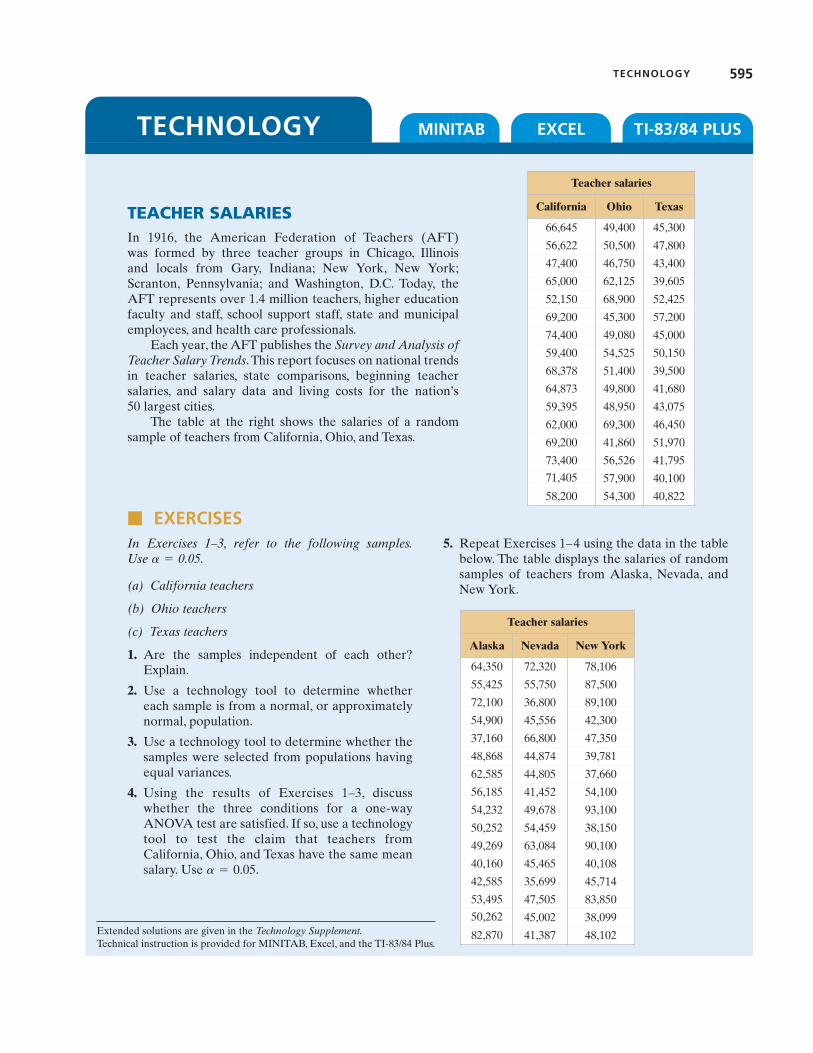
MINITAB EXCEL TI-83/84 PLUS
TECHNOLOGY 595
TECHNOLOGY
Extended solutions are given in the Technology Supplement.Technical instruction is provided for MINITAB, Excel, and the TI-83/84 Plus.
In Exercises 1–3, refer to the following samples.Use
(a) California teachers
(b) Ohio teachers
(c) Texas teachers
1. Are the samples independent of each other?Explain.
2. Use a technology tool to determine whethereach sample is from a normal, or approximatelynormal, population.
3. Use a technology tool to determine whether thesamples were selected from populations havingequal variances.
4. Using the results of Exercises 1–3, discusswhether the three conditions for a one-wayANOVA test are satisfied. If so, use a technologytool to test the claim that teachers fromCalifornia, Ohio, and Texas have the same meansalary. Use
5. Repeat Exercises 1–4 using the data in the tablebelow. The table displays the salaries of randomsamples of teachers from Alaska, Nevada, andNew York.
a = 0.05.
a = 0.05.
# EXERCISES
TEACHER SALARIESIn 1916, the American Federation of Teachers (AFT) was formed by three teacher groups in Chicago, Illinois and locals from Gary, Indiana; New York, New York;Scranton, Pennsylvania; and Washington, D.C. Today, theAFT represents over 1.4 million teachers, higher educationfaculty and staff, school support staff, state and municipalemployees, and health care professionals.
Each year, the AFT publishes the Survey and Analysis ofTeacher Salary Trends.This report focuses on national trendsin teacher salaries, state comparisons, beginning teachersalaries, and salary data and living costs for the nation’s 50 largest cities.
The table at the right shows the salaries of a random sample of teachers from California, Ohio, and Texas.
Teacher salaries
California Ohio Texas
66,645 49,400 45,300
56,622 50,500 47,800
47,400 46,750 43,400
65,000 62,125 39,605
52,150 68,900 52,425
69,200 45,300 57,200
74,400 49,080 45,000
59,400 54,525 50,150
68,378 51,400 39,500
64,873 49,800 41,680
59,395 48,950 43,075
62,000 69,300 46,450
69,200 41,860 51,970
73,400 56,526 41,79571,405 57,900 40,100
58,200 54,300 40,822
Teacher salaries
Alaska Nevada New York
64,350 72,320 78,106
55,425 55,750 87,500
72,100 36,800 89,100
54,900 45,556 42,300
37,160 66,800 47,350
48,868 44,874 39,781
62,585 44,805 37,660
56,185 41,452 54,100
54,232 49,678 93,100
50,252 54,459 38,150
49,269 63,084 90,100
40,160 45,465 40,108
42,585 35,699 45,714
53,495 47,505 83,85050,262 45,002 38,099
82,870 41,387 48,102