10. Algorithm Design Techniquesmouhoubm/=postscript/=c3620/chap10.pdf · 10. Algorithm Design...
47
10. Algorithm Design Techniques 10. Algorithm Design Techniques 10.1 Greedy algorithms 10.2 Divide and conquer 10.3 Dynamic Programming 10.4 Randomized Algorithms 10.5 Backtracking Algorithms Malek Mouhoub, CS340 Fall 2002 1
-
Upload
vuongxuyen -
Category
Documents
-
view
221 -
download
1
Transcript of 10. Algorithm Design Techniquesmouhoubm/=postscript/=c3620/chap10.pdf · 10. Algorithm Design...

10. Algorithm Design Techniques
10. Algorithm Design Techniques
10.1 Greedy algorithms
10.2 Divide and conquer
10.3 Dynamic Programming
10.4 Randomized Algorithms
10.5 Backtracking Algorithms
Malek Mouhoub, CS340 Fall 2002 1

10. Algorithm Design Techniques
Optimization Problem
� In an optimization problem we are given a set of constraints
and an optimization function.
� Solutions that satisfy the constraints are called feasible
solutions.
� A feasible solution for which the optimization function has the
best possible value is called an optimal solution.
Malek Mouhoub, CS340 Fall 2002 2

10. Algorithm Design Techniques
Loading Problem
A large ship is to be loaded with cargo. The cargo is containerized, and all containers
are the same size. Different containers may have different weights. Let �� be the
weight of the ith container, � � � � �. The cargo capacity of the ship is �. We wish
to load the ship with the maximum number of containers.
� Formulation of the problem :
– Variables : �� (� � � � �) is set to � if the container � is not to be loaded
and � in the other case.
– Constraints :
��������� � �.
– Optimization function :
�������
� Every set of ��s that satisfies the constraints is a feasible solution.
� Every feasible solution that maximizes
������� is an optimal solution.
Malek Mouhoub, CS340 Fall 2002 3

4.1 Greedy Algorithms
4.1 Greedy Algorithms
� Greedy algorithms seek to optimize a function by making
choices (greedy criterion) which are the best locally but do not
look at the global problem.
� The result is a good solution but not necessarily the best one.
� The greedy algorithm does not always guarantee the optimal
solution however it generally produces solutions that are very
close in value to the optimal.
Malek Mouhoub, CS340 Fall 2002 4

4.1 Greedy Algorithms
Huffman Codes
� Suppose we have a file that contains only the characters a, e, i,
s, t plus blank spaces and newlines.
– 10 a, 15 e, 12 i, 3 s, 4 t, 13 blanks, and one newline.
– Only 3 bits are needed to distinguish between the above
characters.
– The file requires 174 bits to represent.
� Is it possible to provide a better code and reduce the total
number of bits required ?
Malek Mouhoub, CS340 Fall 2002 5

4.1 Greedy Algorithms
Huffman Codes
� Yes. We can allow the code length to vary from character to
character and to ensure that the frequently occurring characters
have short codes.
� If all the characters occur with the same frequency, then there
are not likely to be any savings.
� The binary code that represents the alphabet can be
represented by a binary tree.
Malek Mouhoub, CS340 Fall 2002 6

4.1 Greedy Algorithms
Huffman Codes
a e i s t sp nl
Representation of the original code in a tree
� The representation of each character can be found by starting at the
root and recording the path, using a 0 to indicate the left branch and a
1 to indicate the right branch.
� If character �� is at depth �� and occurs �� times, then the cost of the
code is equal to
�����.
Malek Mouhoub, CS340 Fall 2002 7

4.1 Greedy Algorithms
Huffman Codes
� newline symbol is an only child and can be placed one level
higher at its parent.
a e i s t sp
nl
A slightly better tree
� Cost using the new full tree = 173.
Malek Mouhoub, CS340 Fall 2002 8

4.1 Greedy Algorithms
Huffman Codes
� Goal : Find the full binary tree of minimum total cost where all
characters are contained in the leaves.
s nl
i
a
t
spe
Optimal prefix code
� Cost = 146
� How is the coding tree constructed ?
– Huffman’s Algorithm
Malek Mouhoub, CS340 Fall 2002 9
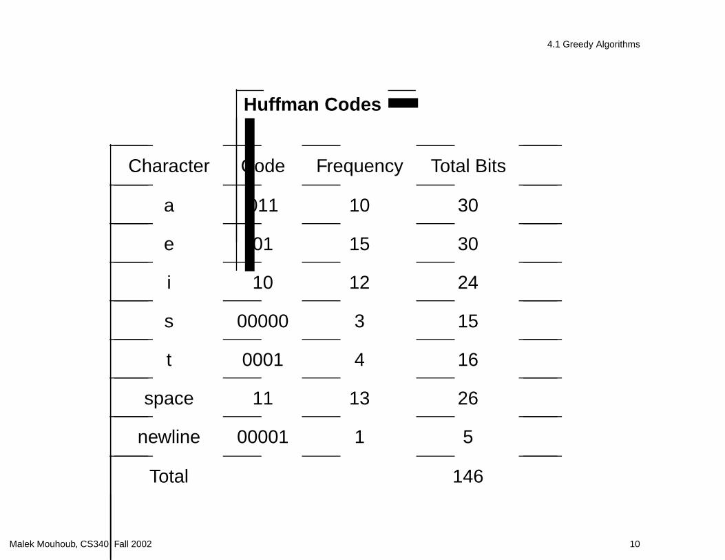
4.1 Greedy Algorithms
Huffman Codes
Character Code Frequency Total Bits
a 011 10 30
e 01 15 30
i 10 12 24
s 00000 3 15
t 0001 4 16
space 11 13 26
newline 00001 1 5
Total 146
Malek Mouhoub, CS340 Fall 2002 10

4.1 Greedy Algorithms
Huffman’s Algorithm
� Assuming that the number of characters is C, Huffman’s
algorithm can be described as follows :
1. At the beginning of the algorithm, there are C single-node
trees, one for each character.
2. The weight of a tree is equal to the sum of the frequencies of
its leaves.
3. C-1 times, select the two trees, �� and ��, of smallest
weight, breaking ties arbitrary, and form a new tree with
subtrees �� and ��.
4. At the end of the algorithm there is one tree, and this is the
optimal Huffman coding tree.
Malek Mouhoub, CS340 Fall 2002 11

4.1 Greedy Algorithms
a e i s t sp nl10 15 12 3 4 13 1
a e i stsp nl10 15 12 13 4
T14
T6
T5
T3
T2
T1
s
T4
a
e i
t
sp
nl
58
Malek Mouhoub, CS340 Fall 2002 12

4.1 Greedy Algorithms
Machine Scheduling
� We are given � tasks and an infinite supply of machines on which
these tasks can be performed.
� Each task has a start time �� and a finish time ��, �� � ��, ���� ��� is
the processing interval for task �.
� A feasible task-to-machine assignment is an assignment in which no
machine is assigned two overlapping tasks.
� An optimal assignment is a feasible assignment that utilizes the
fewest number of machines.
Malek Mouhoub, CS340 Fall 2002 13

4.1 Greedy Algorithms
Machine Scheduling
� We have 7 tasks :
task a b c d e f g
start 0 3 4 9 7 1 6
finish 2 7 7 11 10 5 8
� Feasible assignment that utilizes 7 machines :
���, ��, � � �, � ��.
� Is it the optimal assignment ?
Malek Mouhoub, CS340 Fall 2002 14

4.1 Greedy Algorithms
Machine Scheduling
� A greedy way to obtain an optimal task assignment is to assign the
tasks in stages, one task per stage and in nondecreasing order of task
start times.
� A machine is called old if at least one task has been assigned to it.
� If a machine is not old, it is new.
� For machine selection, we use the following criterion :
– If an old machine becomes available by the start time of the task to
be assigned, assign the task to this machine; if not, assign it to the
new machine.
Malek Mouhoub, CS340 Fall 2002 15

4.1 Greedy Algorithms
Scheduling Problem
� We are given non preemptive jobs ��� � � � � �� , all with known
running times ��� ��� � � � � �� , respectively. We have a single
processor.
� Problem: what is the best way to schedule these jobs in order to
minimize the average completion time ?
� Example :
Job �� �� �� ��Time 15 8 3 10
� Solution 1 : ��� ��� ��� ��. Average completion time : 25.
� Optimal Solution : ��� ��� ��� ��. Average completion time : 17.75.
Malek Mouhoub, CS340 Fall 2002 16

4.1 Greedy Algorithms
Scheduling Problem
� Formulation of the problem :
– � jobs ��� � � � � � ��� with running times ��� � � � � � ���
respectively.
– Total cost : � ���
����� � � � �����
� �� � ����
��� ��� ���
��� ����
� The first sum is independent of the job ordering. Only the
second sum affects the total cost.
� Greedy criterion : Arrange jobs by smallest running time first.
Malek Mouhoub, CS340 Fall 2002 17

4.1 Greedy Algorithms
Scheduling Problem
Multiprocessor case
� non preemptive jobs ��� � � � � �� , with running times
��� ��� � � � � �� respectively, and a number � of processors.
� We assume that the jobs are ordered, shortest running time first.
� Example :
Job �� �� �� �� �� �� �� � �
Time 3 5 6 10 11 14 15 18 20
� Greedy criterion : start jobs in order cycling through processors.
� The solution obtained is optimal however we can have many optimal
orderings.
Malek Mouhoub, CS340 Fall 2002 18

4.1 Greedy Algorithms
Loading Problem
� Using the greedy algorithm the ship may be loaded in stages;
one container per stage.
� At each stage, the greedy criterion used to decide which
container to load is the following :
– From the remaining containers, select the one with least
weight.
� This order of selection will keep the total weight of the selected
containers minimum and hence leave maximum capacity for
loading more containers.
Malek Mouhoub, CS340 Fall 2002 19

4.1 Greedy Algorithms
Loading Problem
� Suppose that :
– � � �,
– ���� � � � � �� � ����� ���� ��� �� ���� ��� ��� ���,
– and � � ��.
� When the greedy algorithm is used, the containers are considered for
loading in the order 7,3,6,8,4,1,5,2.
� Containers 7,3,6,8,4 and 1 together weight 390 units and are loaded.
� The available capacity is now 10 units, which is inadequate for any of
the remaining containers.
� In the greedy solution we have :
���� � � � � �� � ��� �� �� �� �� �� �� �� and
��� � �.
Malek Mouhoub, CS340 Fall 2002 20

4.1 Greedy Algorithms
0/1 Knapsack Problem
� In the 0/1 knapsack problem, we wish to pack a knapsack (bag or sack) with a capacity of �.
� From a list of � items, we must select the items that are to be packed into the knapsack.
� Each object � has a weight �� and a profit �� .
� In a feasible knapsack packing, the sum of the weights of the packed objects does not
exceed the knapsack capacity :
�����
���� � � and �� � �� �� � � � � �
� An optimal packing is a feasible one with maximum profit :
maximize
�����
����
� The 0/1 knapsack problem is a generalization of the loading problem to the case where the
profit earned from each container is different.
Malek Mouhoub, CS340 Fall 2002 21

4.1 Greedy Algorithms
0/1 Knapsack Problem
� Several greedy strategies for the 0/1 knapsack problem are possible.
� In each of these strategies, the knapsack is packed in several stages. In each
stage one object is selected for inclusion into the knapsack using a greedy
criterion.
� First possible criterion : from the remaining objects, select the object with the
maximum profit that fits into the knapsack.
� This strategy does not guarantee an optimal solution.
� Example : � � �� � � ����� ��� ���� � � ���� ��� ���� � � ���.
� Solution using the above criterion : � � ��� �� ��, profit = 20.
� Optimal solution : � � ��� �� ��, profit = 30.
Malek Mouhoub, CS340 Fall 2002 22

4.1 Greedy Algorithms
0/1 Knapsack Problem
� Second criterion : greedy on weight
– From the remaining objects, select the one that has minimum
weight and also fits into the knapsack.
� This criterion does not yield in general to an optimal solution.
� Example : � �� � ���� ��� � � �� ���� � � �.
� Solution : � ��� � inferior to the solution : � ��� �.
Malek Mouhoub, CS340 Fall 2002 23

4.1 Greedy Algorithms
0/1 Knapsack Problem
� Third criterion : greedy on the profit density ����. From the
remaining objects, select the one with maximum ���� that fits
into the knapsack.
� This strategy does not guarantee optimal solutions either.
� Example : � �� � ���� �� �� � � ���� �� � and
� � ��.
Note : The 0/1 knapsack problem is an NP-hard problem. This is the
reason why we cannot find a polynomial-time algorithm to solve it.
Malek Mouhoub, CS340 Fall 2002 24

10.2 Divide and Conquer
10.2 Divide and Conquer
To solve a large instance :
1. Divide it into two or more smaller instances.
2. Solve each of these smaller problems, and
3. combine the solutions of these smaller problems to obtain the
solution to the original instance.
The smaller instances are often instances of the original problem
and may be solved using the divide-and-conquer strategy
recursively.
Malek Mouhoub, CS340 Fall 2002 25
10.2 Divide and Conquer
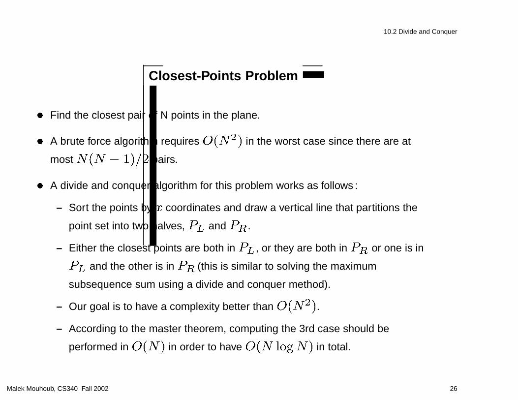
Closest-Points Problem
� Find the closest pair of N points in the plane.
� A brute force algorithm requires �� in the worst case since there are at
most � �� pairs.
� A divide and conquer algorithm for this problem works as follows :
– Sort the points by � coordinates and draw a vertical line that partitions the
point set into two halves, �� and ��.
– Either the closest points are both in ��, or they are both in �� or one is in
�� and the other is in �� (this is similar to solving the maximum
subsequence sum using a divide and conquer method).
– Our goal is to have a complexity better than ��.
– According to the master theorem, computing the 3rd case should be
performed in � in order to have � �� in total.
Malek Mouhoub, CS340 Fall 2002 26

10.2 Divide and Conquer
Closest-Points Problem
� The brute force algorithm to perform the 3rd case requires ��. Why ?
� To do better, one way consists in the following :
1. Compute Æ � ��� �� �.
2. We need then to compute � only if � improves on Æ. The two points that
define � must be within Æ of the dividing line. This area is general
refereed as a strip.
3. The above observation limits in general the number of points that need to be
considered. For large points sets that are uniformly distributed, the number
of points that are expected to be in the strip is of order ��
in
average. The brute force calculation on these points can be performed in
�.
4. However, in the worst case all the points could be in the strip which requires
�� to expect all the points.
5. Can we do better ?
Malek Mouhoub, CS340 Fall 2002 27
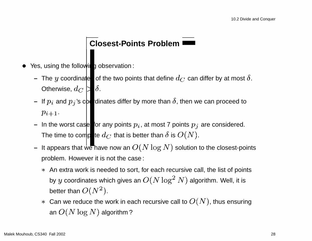
10.2 Divide and Conquer
Closest-Points Problem
� Yes, using the following observation :
– The � coordinates of the two points that define � can differ by at most Æ.
Otherwise, � � Æ.
– If �� and �� ’s coordinates differ by more than Æ, then we can proceed to
����.
– In the worst case, for any points ��, at most 7 points �� are considered.
The time to compute � that is better than Æ is �.
– It appears that we have now an � �� solution to the closest-points
problem. However it is not the case :
� An extra work is needed to sort, for each recursive call, the list of points
by � coordinates which gives an � �� � algorithm. Well, it is
better than ��.
� Can we reduce the work in each recursive call to �, thus ensuring
an � �� algorithm ?
Malek Mouhoub, CS340 Fall 2002 28

10.2 Divide and Conquer
Closest-Points Problem
� Yes. We can maintain two lists. One is the point list sorted by �
coordinate, and the other is the point list sorted by � coordinate. Let’s
call these lists � and �, respectively.
� First we split � in the middle. Once the dividing line is known, we step
through � sequentially, placing each element in �� or �� as
appropriate.
� When the recursive calls return, we scan through the � list and discard
all the points whose � coordinates are not within the strip. The
remaining points are guaranteed to be sorted by their � coordinates.
� This strategy ensures that the entire algorithm is �� �� �,
because only �� � extra work is performed.
Malek Mouhoub, CS340 Fall 2002 29
10.3 Dynamic Programming
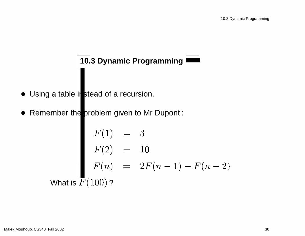
10.3 Dynamic Programming
� Using a table instead of a recursion.
� Remember the problem given to Mr Dupont :
� ��� � �
� ��� � ��
� �� � �� �� ��� � �� ��
What is � �����?
Malek Mouhoub, CS340 Fall 2002 30

10.3 Dynamic Programming
1st Method
Translate the mathematical formula to a recursive algorithm.
if (n==1) � return 3; �
else
if (n==2) �return 10;�
else � return 2 � f(n-1) - f(n-2); �
Malek Mouhoub, CS340 Fall 2002 31

10.3 Dynamic Programming
Analysis of the 1st method
� � ��� � � �� � �� � � �� � ��
� This is a Fibonacci function : � ��� � �� ��
� Complexity of the algorithm : ���� �� � (exponential).
Malek Mouhoub, CS340 Fall 2002 32

10.3 Dynamic Programming
2nd Method
� Use an array to store the intermediate results.
int f[n+1];
f[1]=3;
f[2]=10;
for(i=3;i¡=n;i++)
f[i] = 2 �f[i-1] - f[i-2];
return t[n];
� What is the complexity in this case ?
� What is the disadvantage of this method ?
Malek Mouhoub, CS340 Fall 2002 33

10.3 Dynamic Programming
3rd Method
� There is no reason to keep all the values, only the last 2.
if (n==1) return 3;
last = 3;
current = 10;
for (i=3;i��n;i++) �
temp = current;
current = 2�current - last;
last = temp; �
return current;
� What is the advantage of this method comparing to the 2nd
one ?
Malek Mouhoub, CS340 Fall 2002 34

10.3 Dynamic Programming
Fibonacci Numbers
� We can do use the same method to compute Fibonacci
numbers.
� To compute �� , all that is needed is ���� and ����, we
only need to record the two most recently computed Fibonacci
numbers. This requires an algorithm in ����.
Malek Mouhoub, CS340 Fall 2002 35

10.3 Dynamic Programming
Dynamic Programming for Optimization Problems
� In dynamic programming, as in greedy method, we view the
solution to a problem as the result of a sequence of decisions.
� In the greedy method, we make irrevocable decisions one at a
time using a greedy criterion. However in dynamic
programming, we examine the decision sequence to see
whether an optimal decision sequence contains optimal
decision subsequences.
Malek Mouhoub, CS340 Fall 2002 36

10.3 Dynamic Programming
0/1 Knapsack Problem
� In the case of the 0/1 Knapsack problem, we need to make decisions on the
values of ��� � � � � ��.
� When optimal decision sequences contain optimal decision subsequences, we
can establish recurrence equations, called dynamic-programming recurrence
equations that enable us to solve the problem in an efficient way.
� Let ��� � denote the value of an optimal solution to the knapsack instance
with remaining capacity � and remaining objects �� �� �� � � � � � :
��� � ��
�� if � � ��
� � � � � ��
��� � ��
������� �� �� ��� �� � � �� � ��� if � � ��
��� �� � � � � � ��
Malek Mouhoub, CS340 Fall 2002 37
10.3 Dynamic Programming
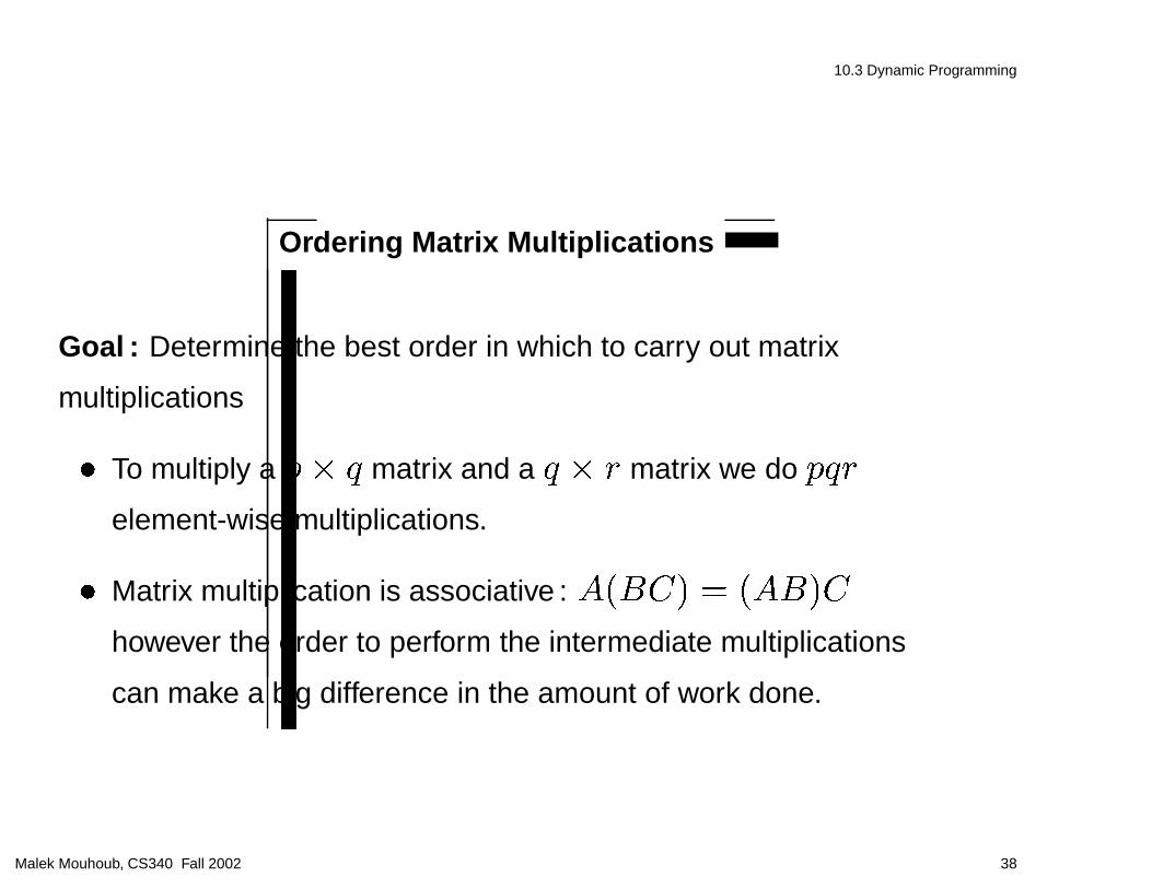
Ordering Matrix Multiplications
Goal : Determine the best order in which to carry out matrix
multiplications
� To multiply a �� � matrix and a � � � matrix we do ���
element-wise multiplications.
� Matrix multiplication is associative : ����� � �����
however the order to perform the intermediate multiplications
can make a big difference in the amount of work done.
Malek Mouhoub, CS340 Fall 2002 38

10.3 Dynamic Programming
Ordering Matrix Multiplications
Example
We want to multiply the following arrays :
�� ������ � �������� � ��������� � ��������
How many multiplications are done for each ordering ?
1. ������������ ������������������������ � ��� ���
2. ������������ ������� � ������ � ������ � ��� ��
3. ������������ ����������������������� � ��� ���
4. ������������ ������� � ������ � ������ � �� ���Malek Mouhoub, CS340 Fall 2002 39

10.3 Dynamic Programming
Ordering Matrix Multiplications
General Problem :
Suppose we are given matrices ��� ��� � � � � �� where the
dimensions of �� are ����� � ��� (for � � � � ). What is the
optimal way (ordering) to compute :
����� � ��������� � ���� �������� � ���Malek Mouhoub, CS340 Fall 2002 40
10.3 Dynamic Programming
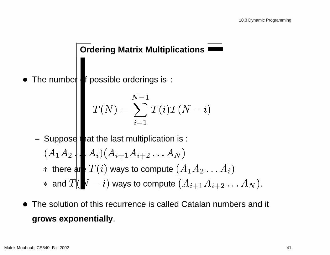
Ordering Matrix Multiplications
� The number of possible orderings is :� ��� �
�������
� ���� �� � ��
– Suppose that the last multiplication is :
����� � � � ���������� � � � �� �
� there are � ��� ways to compute ����� � � � ���
� and � �� � �� ways to compute ������� � � � �� �.
� The solution of this recurrence is called Catalan numbers and it
grows exponentially.
Malek Mouhoub, CS340 Fall 2002 41

10.3 Dynamic Programming
Ordering Matrix Multiplications
� ��� ���� is the number of multiplications required to
multiply ��� ��� � �����
� ���� ������� ����� � is the last multiplication.
� The number of multiplications required is :
��� � �������� � ��� ���������
� The number of multiplications in an optimal ordering is :
����� �� �
���������� �������������� ������������� ���
Malek Mouhoub, CS340 Fall 2002 42

10.4 Randomized Algorithms
10.4 Randomized Algorithms
� A randomized algorithm is an algorithm where a random
number is used to make a decision at least once during the
execution of the algorithm.
� The running time of the algorithm depends not only on the
particular input, but also on the random numbers that occur.
Malek Mouhoub, CS340 Fall 2002 43

10.4 Randomized Algorithms
Primality Testing
� Problem : Test whether or not a large number is prime ?
� The obvious method requires an algorithm of complexity
��
��. However nobody knows how to test whether a �-digit
number � is prime in time polynomial in �.
� Fermat’s Lesser Theorem :
If � is prime, and � � � � � , then ���� � ��mod � �Malek Mouhoub, CS340 Fall 2002 44

10.4 Randomized Algorithms
Primality Testing
� Using Fermat’s Lesser Theorem, we can write an algorithm for primality testing
as follows :
1. Pick � � � � � � at random.
2. If ���� � �mod � declare that is “probably” prime, Otherwise
declare that is definitely not prime.
� Example : if � ���, and � � �, we find that ���� � ��mod ����
� If the algorithm happens to choose � � �, it will get the correct answer for
� ���.
� There are some numbers that fool even this algorithm for most choices of �.
� One such set of numbers is known as the Carmichael numbers. They are not
prime but satisfy ���� � �mod for all � � � � that are relatively
prime to . the smallest such number is 561.
Malek Mouhoub, CS340 Fall 2002 45

10.4 Randomized Algorithms
Primality Testing
� We need an additional test to improve the chances of not
making an error.
� Theorem : If � is prime and � � � � � , the only solutions to
�� � ��mod � � are � � �� � � �.
� Therefore, if at any point in the computation of �����mod ��
we discover violation of this theorem, we can conclude that � is
definitely not prime.
Malek Mouhoub, CS340 Fall 2002 46

10.5 Backtracking
10.5 Backtracking
� Backtracking is a systematic way to search for the solution to a problem.
� This method attempts to extend a partial solution toward a complete solution.
� In backtracking, we begin by defining a solution space or search space for the problem.
� For the case of the 0/1 knapsack problem with� objects, a reasonable choice for the solution space is the set of �� 0/1
vectors of size�. This set represents all possible ways to assign the values 0 and 1 to�.
� The next step is to organize the solution space so that it can be reached easily. The typical organization is either a graph or a
tree.
� Once we have defined an organization for the solution space, this space is searched in a depth-first manner beginning at a start
node.
� The start node is both a live node and the E-node (expansion node).
� From this E-node, we try to move to a new node.
� If such a move is possible, the new node becomes a live node and also becomes the new E-node. The old E-node remains a live
node.
� If we cannot move to a new node, the current E-node dies and we move back to the most recently seen live node that remains.
This live node becomes the new E-node.
� The search terminates when we have found the answer or when we run out of live nodes to back up to.
Malek Mouhoub, CS340 Fall 2002 47