1 Wallet Study Reader’s Digest, over a period of years, “lost” more than 1,100 wallets in...

1

Wallet Study

Reader’s Digest, over a period of years, “lost” more than 1,100 wallets in various cities. Each wallet contained $50 in local currency and a name and phone number so it could be returned. The wallets were dropped in various places (phone booths, sidewalks, restaurants, etc.).

2

Wallets ReturnedNorway 100% Denmark 100%

Singapore 90% New Zealand 83%

Finland 80% Scotland 80%

Australia 70% Japan 70%

South Korea 70% Spain 70%

Austria 70% Sweden 70%

U.S. 67% England 67%

India 65% Canada 64%

France 60% Brazil 60%

Netherlands 60% Thailand 55%

Belgium 50% Taiwan 50%

Malaysia 50% Germany 45%

Portugal 45% Argentina 44%

Russia 43% Philippines 40%

Wales 40% Italy 35%

Switzerland 35% Hong Kong 30%

Mexico 21% AVERAGE: 56%

3

U.S. Cities

Wallets Returned Wallets Kept

Seattle 9 1

St. Louis 7 3

Atlanta 5 5

Boston* 7 3

Los Angeles* 6 4

Houston* 5 5

Greensboro, N.C. 7 3

Las Vegas 5 5

Dayton, Ohio 5 5

Concord, N.H. 8 2

Cheyenne, Wyo. 8 2

Meadville, Pa. 8 2

(*wallets dropped in suburbs of these cities)

4

Neglected Topics

Families

Norms

Social Outputs

5

Families

Families are associations similar to the ones that Putnam and others measure.

If all families were equal, omitting them from analysis would not matter.

But families differ a lot:

1. Presence of one or both parents.

2. Inclusion of siblings, grandparents, cousins.

3. Number of siblings.

6

Norms

Norms are rules that exist independent of enforcement by the government.

One way to view them is as equilibria of games such as the prisoner’s dilemma and the coordination game.

7

THE TAXONOMY• (1) Bilateral Costly Sanctions. One other

person incurs the cost of punishing you.

• (2) Multilateral Costly Sanctions. Many other people incur the cost of punishing you.

• (3) Automatic Sanctions. Crashing into a driver on the road.

• (4) Guilt. You feel bad about your sin, even though nobody else knows or cares.

• (5) Shame. You feel you have lowered yourself. (disapproval)

• (6) Informational Sanctions. Your action conveys unfavorable info about yourself.

8

SIGNALLING GAME

• 1. Nature chooses 90 percent of workers to be steady, producing x, and 10 percent wild, producing x-y.

• 2. Each worker decides to marry or not. Marriage adds m to the utility of the steady, and -z to the wild.

• 3. Employers offer wages conditional on marriage.

• (Spence won the Nobel Prize in 2001 for signalling)

9

EQUILIBRIUM

• If z>y, so wild workers hatred of marriage is greater than their inferiority in output, then they stay single and the steady get married.

• If z<.9y, everyone gets married, and the wage is pooling. There is a norm of marriage, enforced by an informational penalty.

• In between is a mixed-strategy equilibrium.

10

WHAT CAN GOVERNMENT DO?

• 1. Provide supplemental punishments.

• 2. Provide info on who did what.

• 3. Be careful about interfering with private sanctions.

• 4. Supplement incentives for private sanctions.

• 5. Help in norm creation.

• 6. Fight bad norms.

11

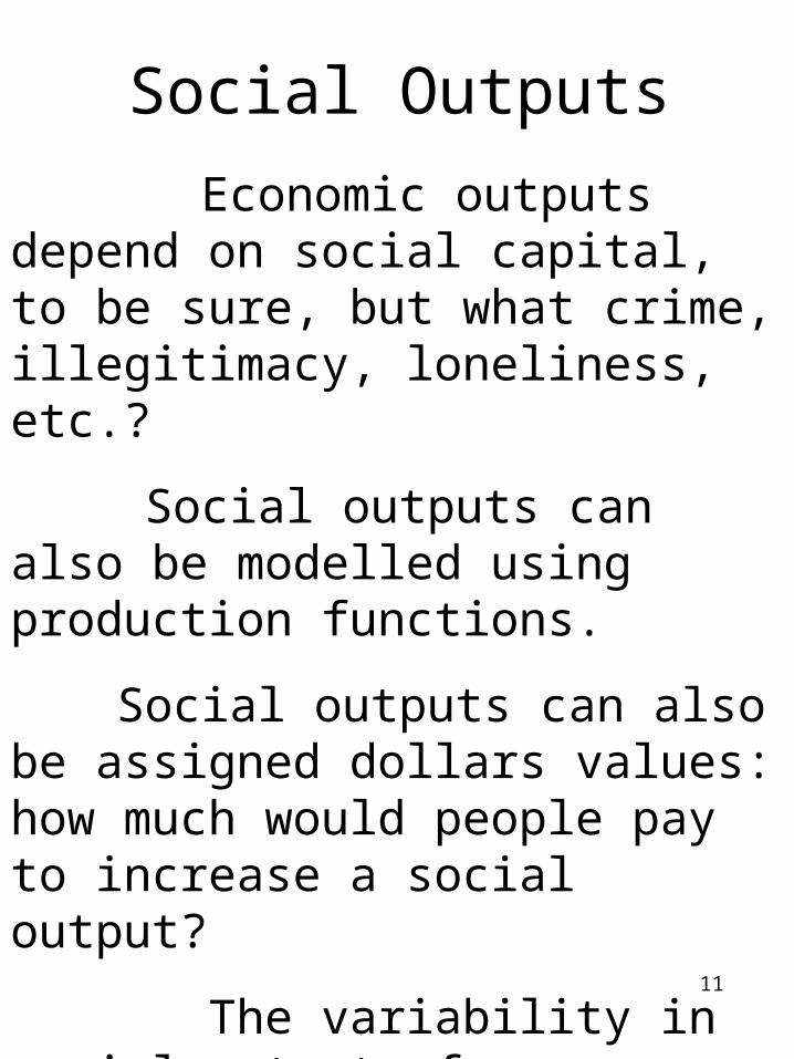
Social Outputs

Economic outputs depend on social capital, to be sure, but what crime, illegitimacy, loneliness, etc.?

Social outputs can also be modelled using production functions.

Social outputs can also be assigned dollars values: how much would people pay to increase a social output?

The variability in social outputs from differing levels of social capital may be much greater than the variability in economic outputs.

12

Insert a tex slide table

Go to the State data tables

13

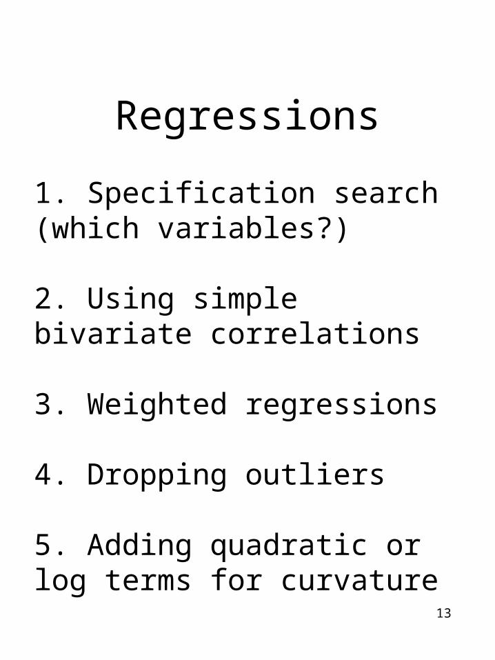
Regressions

1. Specification search (which variables?)

2. Using simple bivariate correlations

3. Weighted regressions

4. Dropping outliers

5. Adding quadratic or log terms for curvature

14

Available Data

pop malework murder cartheft illegit divorce metro retired midage unemp teachsal homeown income bachelor abortion black southern churchm voting

15

Bivariate Correlations with the Murder Rate

malework -.25cartheft .71illegit .79divorce .03metro .27retired -.03midage .14unemp .38teachsal .15homeown -.52income .23

bachelor .32abortion .84black .77southern .38churchm .06voting -.27

16

Source: Robert Putnam: Bowling Alone, “Selected statistical trend data”http://www.bowlingalone.com/data.php3 (12/8/01)

State Comprehensive social capital index II

501(c)(3) organizations per capita, 1989

GSS: Mean number of group memberships

GSS: "Most people can be trusted"

State Comprehensive social capital index II

501(c)(3) organizations per capita, 1989

GSS: Mean number of group memberships

GSS: "Most people can be trusted"

putnam orgs member trust

Average 0.67 2.33 2.10 0.54

Alaska . 2.82 . . Rhode Island -0.06 1.94 1.90 52%DC . . . . Indiana -0.08 1.97 1.87 43%Hawaii . 2.28 . . Oklahoma -0.16 2.17 1.65 39%North Dakota 1.71 2.86 3.29 67% Ohio -0.18 2.00 1.88 41%South Dakota 1.69 2.53 . . California -0.18 2.20 1.69 43%Vermont 1.42 3.57 . 59% Pennsylvania -0.19 1.67 1.91 44%Minnesota 1.32 2.31 2.13 63% Illinois -0.22 2.14 1.72 44%Montana 1.29 2.90 2.69 64% Maryland -0.26 1.91 1.95 42%Nebraska 1.15 2.35 . . Virginia -0.32 1.63 1.82 38%Iowa 0.98 2.42 1.99 56% New Mexico -0.35 1.67 . .New Hampshire 0.77 2.13 1.51 62% New York -0.36 2.14 1.66 40%Wyoming 0.67 2.88 2.35 60% New Jersey -0.40 1.55 1.67 41%Washington 0.65 2.30 2.13 46% Florida -0.47 1.41 1.62 37%Wisconsin 0.59 2.03 1.87 52% Arkansas -0.50 1.60 1.44 29%Oregon 0.57 2.42 1.83 55% Texas -0.55 1.81 1.79 33%Maine 0.53 2.24 . . Kentucky -0.79 1.54 1.51 32%Utah 0.50 1.31 2.46 54% North Carolina -0.82 1.77 1.30 27%Colorado 0.41 2.45 1.95 46% West Virginia -0.83 1.62 1.59 30%Kansas 0.38 2.21 2.11 55% South Carolina -0.88 1.42 1.87 34%Connecticut 0.27 2.25 2.05 49% Tennessee -0.96 1.44 1.73 36%Massachusetts 0.22 2.29 1.77 46% Louisiana -0.99 1.30 1.31 33%Missouri 0.10 2.10 1.80 44% Alabama -1.07 1.40 1.65 23%Idaho 0.07 2.07 . . Georgia -1.15 1.43 1.84 38%Arizona 0.06 1.67 1.88 47% Mississippi -1.17 1.18 1.62 17%Michigan 0.00 1.56 1.89 51% Nevada -1.43 1.49 . .Delaware -0.01 2.35 . .

18

Bivariate Correlations with “putnam” Social Capital

malework .58murder -.74cartheft -.45illegit -.56divorce -.35metro -.36retired .15midage -.05unemp -.44teachsal -.13homeown .05income .09

bachelor .34abortion -.30black -.71southern -.62churchm -.02voting .69

19

Different Measures Murder = putnam -2.75 (7.55) R2 = .55 N = 48

Murder = trust -.16 (6.03) R2 = .48 N=41

Murder = orgs -3.44 (5.17) R2 = .35 N=50

Murder = member -1.06 (3.35) R2 = .22 N=40

Murder = putnam orgs trust member -2.60 .08 -.03 .91

(1.89) (0.07) (0.47) (0.71)R2 = .52 N=40

20

Weighting

Murder = putnam income -2.69(7.51) -.00012(1.75)

Murder = putnam income -2.48(5.58) -.00014(2.05) (weight = pop)

Murder = putnam income -2.46(8.00) -.00018(2.38) (weight = 1/pop)

Murder = putnam income -2.69(9.97) -.00012(1.60) (White robust standard errors)

21

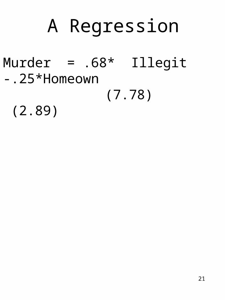
A Regression

Murder = .68* Illegit -.25*Homeown (7.78) (2.89)

22

Residuals from Illegit,Homeown

state v1 1. AL 1.313196 2. AK -.0083414 3. AZ -3.002368 4. AR -.3776368 5. CA .1270525 6. CO 4.011913 7. CT .6871804 8. DE -8.302368 9. DC 20.62919 10. FL -3.582326 11. GA -1.276142 12. HA -4.394481 13. ID 5.293575 14. IL .9854771 15. IN -.028383 16. IA -.3358477 17. KA 2.801039 18. KE .0886737 19. LA -3.010255 20. ME -3.217509 21. MD 1.957757 22. MA .5488002 23. MI .6701256 24. MN 1.619589 25. MS -5.27337

26. MO -.1145223 27. MT -.0974675 28. NE 2.119589 29. NV 1.030039 30. NH 1.85349 31. NJ .9795045 32. NM -5.145649 33. NY -4.276142 34. NC 1.391659 35. ND -1.135848 36. OH -3.414522 37. OK -.6083413 38. OR -.7113263 39. PA -1.172947 40. RI -5.171453 41. SC -3.259298 42. SD -4.209833 43. TN .614687 44. TX 1.582491 45. UT 9.338348 46. VT -1.134354 47. VA 2.237926 48. WA 1.193363 49. WV -1.231369 50. WI .0302502 51. WY 1.387181

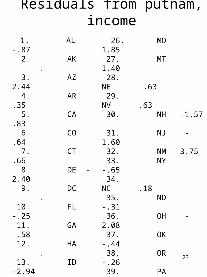
23

Residuals from putnam, income

1. AL -.87 2. AK . 3. AZ 2.44 4. AR .35 5. CA .83 6. CO .64 7. CT .66 8. DE -2.40 9. DC . 10. FL -.25 11. GA -.58 12. HA . 13. ID -2.94 14. IL 2.70 15. IN 1.76 16. IA -1.22 17. KA 1.26 18. KE -3.59 19. LA 4.01 20. ME -2.42 21. MD 4.29 22. MA -1.98 23. MI 1.78 24. MN .974 25. MS 1.86

26. MO 1.85 27. MT 1.40 28. NE .63 29. NV .63 30. NH -1.57 31. NJ -1.60 32. NM 3.75 33. NY -.65 34. NC .18 35. ND -.31 36. OH -2.08 37. OK -.44 38. OR -.26 39. PA -.62 40. RI -3.05 41. SC -.40 42. SD .11 43. TN .13 44. TX -.35 45. UT -1.59 46. VT .28 47. VA .01 48. WA .42 49. WV -4.27 50. WI -.37 51. WY .87

24

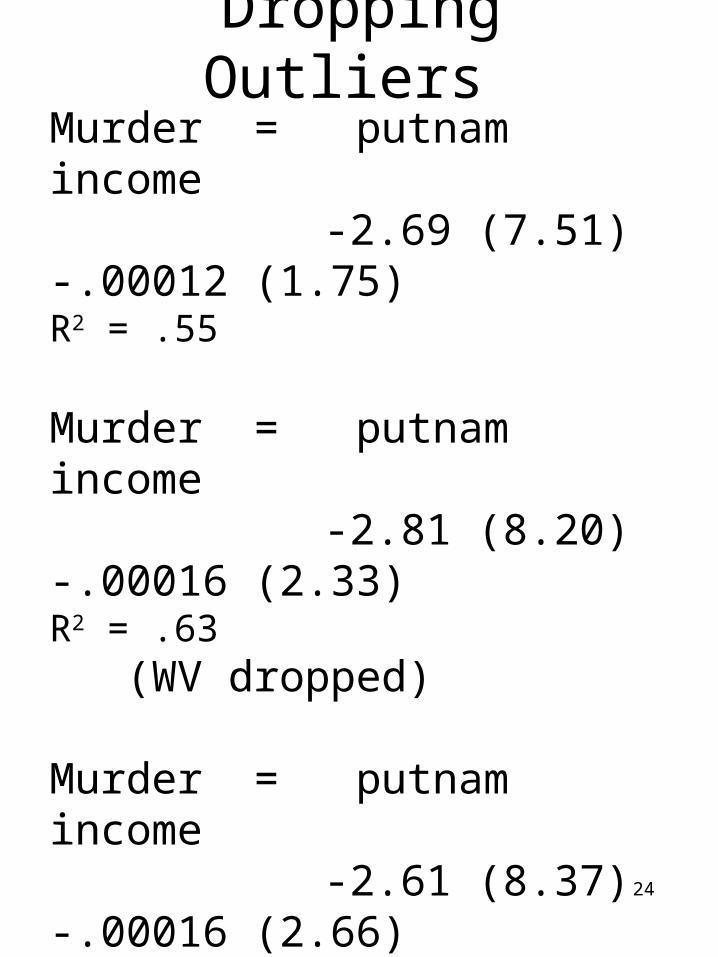
Dropping Outliers

Murder = putnam income -2.69 (7.51) -.00012 (1.75) R2 = .55

Murder = putnam income -2.81 (8.20) -.00016 (2.33) R2 = .63 (WV dropped)

Murder = putnam income -2.61 (8.37) -.00016 (2.66) R2 = .65 (WV,MD,LA dropped)

Not much happens if outliers are dropped.

25

Dropping Outliers

Murder = illegit homeown -0.68 (7.78) -0.25 (2.89) R2 = .67

Murder = illegit homeown -0.37 (7.31) 0.05 (0.98) R2 = .53 (DC dropped)

The effect of illegitimacy becomes smaller, and home ownership becomesinsignificant.

26

Squared and Log Terms

Murder = illegit homeown -0.68 (7.78) -.25 (2.89) R2 = .67

Murder = log(illegit) homeown 19.20 (5.56) -.33 (3.33) R2 = .55

Murder = illegit illegit2 homeown -1.61 .03 -.07 (6.27) (9.14) (1.23)R2 = .88

27

Murder

Regression 1 R 2 = .55

Putnam -2.75 (7.55)


Putnam -1.62 (3.06)Income -0.00028 (2.75)Black 0.15 (3.45)Metro 0.024 (1.18)Southern -1.58 (1.83)

28

Illegitimacy


Putnam -4.23 (4.91)



29

Male Labor Participation


Putnam 2.60 (5.08)


Putnam 2.45 (2.89)Income 0.00012 (0.74)Black 0.007 (0.11)Metro 0.013 (0.42)Southern -0.76 (0.55)

30

Car Theft


Putnam -103.86 (3.53)



31

Aristotle contra Kelvin

Kelvin: ``When you measure what you are speaking about and express it in numbers, you know something about it, but when you cannot express it in numbers your knowledge about is of a meagre and unsatisfactory kind.'’

Aristotle: ``...it is the mark of an educated manto look for precision in each class of things just so far as the nature of the subject admits; it is evidently equally foolish to accept probable reasoning from a mathematician and to demand from a rhetoricianscientific proofs.'’

Kelvin: ``In science there is only physics; all the rest is stamp collecting.'' Kelvin: ``I can state flatly that heavier than air flying machines are impossible.'’

1 Wallet Study Reader’s Digest, over a period of years, “lost” more than 1,100 wallets in...

Documents

Transcript of 1 Wallet Study Reader’s Digest, over a period of years, “lost” more than 1,100 wallets in...