TRENDS IN RAINFALL EXTREMES

RICHARD L. SMITH 1

SUMMARY

Many scientists believe that there is an anthropogenic in uence on the earth's climate.

Most research on this issue has been concerned with an apparent overall increase in tem-

peratures, popularly known as global warming. However, there is also increasing interest

in other forms of climate change which may possibly have anthropogenic origins. One

of these is the hypothesis that overall rainfall levels in the USA are not only increasing,

but that most of the increase derives from extreme events. In this paper, we use extreme

value theory to examine whether there is an increasing trend in the frequency of extreme

one-day precipitation events in the USA. Our data source consists of 187 stations from the

Historical Climatological Network, and initial station-by-station analyses show evidence of

an overall increasing trend but with huge variablity from station to station. To integrate

the data from di�erent stations, we develop a conceptual hierarchical model using geosta-

tistical methods to represent the variability between stations. Our analysis of this model,

however, stops short of a full Bayesian implementation, using an approximate model �t

which allows us to adapt standard geostatistical methods to this setting. The results are

most meaningful when summarized in terms of regional average trends: there is remarkable

homogeneity in the overall trend in rainfall extremes among di�erent regions of the USA.

The conclusion is contrasted with the corresponding result for mean temperatures.

Keywords: Climate change, Extreme value theory, Hierarchical models, Point pro-

cesses, Spatial statistics,

1 Richard L. Smith is Professor, Department of Statistics, University of North Carolina,

Chapel Hill, N.C. 27599-3260; email address rls@email.unc.edu. At the time of writing

this paper he was also a Research Fellow at the Isaac Newton Institute for Mathematical

Science, Cambridge, U.K. The research was supported, in part, by N.S.F. grant DMS-

9705166, by E.P.S.R.C. Visiting Fellowship grant GR-K99015, and by the U.K. Tsunami

Foundation. Thanks are also extended to Tom Karl and Dick Knight of the National

Climatic Data Center for access to the data, to Mark Handcock for a Fortran routine used

to calculate the Mat�ern covariance function, and to Ian Jolli�e for a suggestion related to

section 5(c).

1

1. INTRODUCTION

The topic of global climate change poses many statistical challenges. The vast majority

of studies have concentrated on mean temperature as the primary variable of interest, and

there are many ongoing debates over attribution questions | to what extent the observed

global warming can be \explained" as a consequence of di�erent forcing factors. A very

recent example of this kind of analysis is in Wigley et al. (1998), in which hemispherically

averaged annual mean temperatures were regressed on a number of explanatory variables

including an \anthropogenic" signal representing greenhouse gas and sulfate aeorsol e�ects,

and a \solar" signal determined by variations in solar ux. It was found necessary to

include both kinds of terms in the model, a result which was interpreted as reinforcing the

evidence that anthropogenic e�ects are needed to explain the observed global warming.

In the light of this and much other research on global warming, attention is naturally

turning to other \indicators" of climate change. There is widespread speculation that

other phenomena such as hurricanes and tropical cyclones are also increasing as a conse-

quence of global warming, but there is very little direct evidence to support any such link.

Nevertheless, it is natural enough that climate researchers are trying to �nd evidence of

climate change in variables other than large-scale temperature means.

One of the more serious studies along these lines to have emerged so far is the paper

by Karl et al. (1996). They computed a number of summary statistics for di�erent

measures of climate change and then tested for trend in the annual values, under a null

hypothesis which allowed for the model to be a stationary time series of ARMA form. One

of the most signi�cant results (claimed to have a P-value of less than 0.01) was a series

de�ned as \percentage of the U.S.A. with a much above normal proportion of total annual

precipitation from extreme precipitation events (daily events at or above 2 inches)". Few

details were provided of exactly how this variable was calculated, one obvious diÆculty

being that many of the measuring stations are operative for only a portion of the period

of observation (1910{1996). Nevertheless, the authors claimed a clear increasing trend as

the level of the series rose from around 9% in 1910{1920 to near 11% in the 1990s. The

intended implication was clear: extreme events are becoming more frequent.

In a subsequent paper, Karl and Knight (1998) calculated trends in the proportions of

mean daily precipitation levels that lie within 20 equiprobable subintervals of the spatially

aggregated daily rainfall series. For the top 5% of the range, they found a clear increasing

trend in frequencies. For other 5% intervals near the top end, the trend was increasing but

not as much as in the top 5%. For the middle and low end of the daily precipitation range,

there was little or no trend. These results were shown to hold for precipitation variables

aggregated across the continental U.S.A., but broadly similar results were obtained when

the analysis was repeated on each of nine spatially contiguous subregions. Thus the authors

concluded that there is an overall increasing trend in daily rainfall totals, but the trend is

concentrated at the high end of the distribution, and this pattern of behavior seems fairly

uniform across the U.S.A.

2

In the present author's view, these analyses are convincing enough when assessed on

their own merits, but they raise a number of questions which justify an alternative and

possibly more thorough statistical analysis. Among these questions are:

1. As already remarked, the studies raise questions over exactly how the spatially

aggregated rainfall values were computed, especially in the light of di�erent fractions of

missing data in di�erent time periods. As a result, it is hard to be sure that they represent

truly homogeneous series.

2. The format of the analysis | �rst compute a summary statistics and then look for

trends | makes it hard to translate the results to other variables. For example, suppose we

were interested in investigating trends at a speci�c location or over ranges of precipitation

amounts other than the given 5%-wide quantile intervals. There is no straightforward

method, beyond computing a new summary statistic for the variable of interest.

3. The analysis made no attempt to incorporate the statistical theory of extreme

values, which is arguably the right theory for investigating this type of question. Conse-

quently, it seems unlikely that the analyses are using the data in an optimal way.

This paper presents an alternative analysis which approaches the problem from the

opposite point of view. Instead of �rst computing aggregate statistics and then looking for

trends, we search for trend in individual station values using well-established techniques

of extreme value theory. As is typical for single-station analyses, however, the results,

although supporting the hypothesis of an overall increasing trend, show huge variability

from station to station which makes diÆcult any interpretation of an overall trend in

climate. The second half of the paper discusses ways to combine the results across stations.

A conceptual hierarchical model is presented which allows the extreme value parameters

to vary smoothly over space. We stop short of a full Bayesian implementation, however,

believing that this would be too computationally demanding. Instead, an approximate

form of hierarchical model is proposed, using a normal-normal structure, which has the

advantage that many of the relevant conditional probability calculations can be performed

without recourse to simulation. This model is �tted by the method of maximum likelihood.

As a comparison, the analysis of the rainfall extremes problem is performed in parallel with

a similar, but much easier, analysis of trends in temperature means.

The �nal part of the paper discusses the interpretation of these results. In particular,

we �nd that when interpreted from the point of view of regional averages, the trend in

extreme rainfall quantiles is remarkably homogeneous over di�erent regions of the country,

at about .09% per year over 1951{1996. The analysis sheds no light on the all-important

question of whether the trend is anthropogenic in origin, but by summarizing the results

of the data analysis in such speci�c terms, it is hoped to provide some detailed hypotheses

which may be tested in future analyses using numerical climate models.

3

2. DATA AND METHODOLOGY

The data nominally consist of 87 years' (1910{1996) of daily rainfall values at each

of 187 climate stations spread across the continental U.S.A. The data form part of the

Historical Climatological Network archive prepared by the National Climatic Data Center

in Asheville, North Carolina. Many of the stations were not in operation for the entire

87-year period, and in addition, all the series contain some portions of data missing at

random. As a guide to the likely consequences of missing data, Fig. 1 computes, for

each year of the study, an overall percentage of missing values from all station � day

combinations within that year. The proportion of missing data drops from around 50% in

1910 to about 10% by 1950, and thereafter remains at that level until a small rise in the

1980s.

••••••••••••••••

••

•••••••••••••••••••

•

•••••••••••••••••••••••••••••••••••••••••

••••••••

Year

Per

cent

mis

sing

1920 1940 1960 1980

0

10

20

30

40

50

Fig. 1. Percentage of missing data in the whole network, for each year from 1910 to 1996.

Our single-station analysis is an adaptation of the threshold-based method of Smith

(1989). Suppose we have a long time series consisting of daily values of some scalar variable

| in this case, daily rainfall totals at a single station. Missing values are allowed.

Threshold methods are based on �tting stochastic models to the exceedances over a

high threshold. Davison and Smith (1990) gave a broad discussion of the methodology.

The �rst step in such an analysis is to identify clusters of dependent high values. Accord-

ing to the most popular version of the method, often called the peaks over threshold or

POT method, the peak value within each cluster is picked out so as to create a series of

4

approximately independent values. In the present analysis, clusters were de�ned by the

property that two threshold exceedances within three days of each other are considered

part of the same cluster. De�ning clusters in this way, and throwing out all non-peak

exceedances, reduced the total number of exceedances by approximately 20%, the exact

percentage depending on the threshold chosen. More sophisticated methods of handling

temporal dependence in extreme value analysis are available (e.g. Smith et al. 1997,

Ledford and Tawn 1998), but it would be computationally expensive to apply these to

such a large number of parallel time series, so for the present analysis, this simple form of

declustering was the only allowance made for temporal dependence.

Following Smith (1989), the basic model for threshold exceedances is based on con-

structing a two-dimensional point process f(Ti; Yi)g, where Ti is the time of the ith peak

exceedance and Yi is the value. According to a point-process interpretation of extreme

value theory (Leadbetter et al. 1983), for suÆciently high threshold and suÆciently long

time periods, this two-dimensional point process may be represented as a nonhomogeneous

Poisson process. The intensity of this process is de�ned for all Borel sets if we can de�ne it

on all rectangles of the form A = (t1; t2)� (y;1) where t1 and t2 are time coordinates and

y � u is a given level of the process. Writing t1 = t and t2 = t+ Æt with Æt in�nitesimal,

we write

�(A) = Æt ��1 + �t

(y � �t)

�t

��1=�t

+

; (1)

where x+ = max(x; 0) and �t, �t, �t represent respectively a location parameter, scale

parameter and shape parameter for time t. Allowing these parameters to be time dependent

creates the possibility of introducing covariate e�ects into the analysis.

For a model so de�ned, it is straightforward to write down a likelihood function, and

hence to �nd maximum likelihood estimators. If we observe the process on a time interval

[0; T �], and if on this interval we observe N exceedances at times T1; :::; TN , the likelihood

function is given by

L =

NYi=1

"1

�Ti

�1 + �Ti

(Yi � �Ti)

�Ti

��1=�Ti�1

+

#exp

"�Z T�

0

�1 + �t

(u� �t)

�t

��1=�t

+

dt

#(2)

and maximum likelihood estimators are obtained by maximizing (2). In practice, we

maximize log L and use the observed information matrix to determine standard errors of

the parameter estimates. Also, in practice, the integral in (2) is replaced by a sum of form

Z T�

0

�1 + �t

(u� �t)

�t

��1=�t

+

dt � hXt

�1 + �t

(u� �t)

�t

��1=�t

+

(3)

where the sum is over days t and h is the length of one day in whatever time units are

adopted as a base of the analysis. In the present case we adopt a base time interval of one

year so h = 1

365:25.

5

•

• •

•

•

•

•

A

y

u

t_1 t_20 T

Fig. 2. Illustration of point process representation. The points on the graph represent

times t and values y of exceedances over the threshold u. The set A (consisting of all time

points between t1 = t and t2 = t+ Æt and all values between y and 1) is the set in which

the expected number of points is given by formula (1).

Another feature of this form of representation is that the likelihood function is very

easily adapted to handle missing values, assuming of course that the missing values are

noninformative. If we replace the interval [0; T �] by a union of intervals for which data are

available, then the expression is the same except that the integral in (2) or the sum in (3)

are replaced by an integral or sum over the available period of data. For the rest of the

paper, it will be assumed without further comment that such adjustment has been made

wherever there are missing data.

With the rainfall data for a single station, the only covariate of interest is time, and

the model adopted is of form

�t = �0evt ; �t = �0e

vt ; �t = �0; (4)

where �0; �0; �0 are constants for each station and

vt = �1t+

PXp=1

f�2p cos(!pt) + �2p+1 sin(!pt)g; (5)

6

�1 representing a linear trend and the remaining terms in (5) representing periodic e�ects

of frequency !1; :::; !P . In practice, P has been set equal to 2, with !1; !2 corresponding

to one-year and six-month cycles respectively.

The form of model (4){(5) was chosen after initial exploration of the data at a few

selected stations suggested that (a) there is very strong evidence of a seasonal e�ect, but in

all stations examined, this can be modeled with either one or two sinusoidal components,

(b) the evidence for a trend is much less strong, but does seem to be present in some

stations, and (c) a model in which both �t and �t vary with time seems to be both a

better �t and more readily interpretable than one with only �t time dependent, as has been

adopted in previous examples of this methodology, e.g. Smith (1989). The decision to focus

on a linear trend �1t is not motivated by any evidence that the true trend really is linear

in time, but rather as a convenient starting point for study of this question. Concerning

the interpretation of the model de�ned by (1){(5), �rst note that the probability that the

level y is not exceeded during a one-year time period [T; T + 1] is given by

qT (y) = exp

"�Z T+1

T

�1 + �0

�y � �0e

vt

�0evt

���1=�0

+

dt

#; (6)

so that the q-level quantile of the maximum daily rainfall in year T , yT (q) say, is obtained

by solving (6) for y at a given q. If (5) holds with all the sinusoidal terms having periods

which are integer fractions of one year, then it is readily seen that

yT+1(q) = e�1yT (q); (7)

in other words, �1 is intepretable as an \in ation factor" associated with the extreme quan-

tiles of the annual maxima of the daily rainfall values. This relatively simple intepretation

is an additional motivation for writing the model in the form which we have.

3. THRESHOLD SELECTION AND MODEL DIAGNOSTICS

In this section we consider the important question of how to choose the threshold,

and related to that, diagnostics for the �t of the overall model. Threshold selection can be

viewed in decision-theoretic terms, chosen for example to minimize the mean squared error

of an estimated quantile. In recent years a number of ingenious data-based techniques have

been proposed (for example, by Hall and Weissman, 1997), but the practical applicability

of these techniques has still to be demonstrated, especially in models with more complex

structure than simple IID data. In this paper, we take a more pragmatic approach, choosing

thresholds which are low enough to capture a reasonable proportion of the data, and

conducting diagnostic tests to con�rm the �t of the model at those thresholds.

One useful diagnostic is the mean excess over threshold plot, introduced by Davison

and Smith (1990), where it was called the mean residual life plot. For each threshold y

over some base threshold u, the mean of all excesses over y is computed (in other words,

7

for each observation Y over the threshold y, calculate Y � y and then take the mean),

and the result is plotted against y. If the model (1) is correct for the threshold u, then

excesses over the thresholds y � u follow a generalized Pareto distribution (henceforth

GPD), and in this case the plot should be close to a straight line. In practice, the plot

can be hard to interpret because at higher levels of y, the sampling variability of the mean

excess is enormous, so the plot tends to look very unstable. As a guide to interpretation,

however, it is possible to compute pointwise 95% con�dence limits, by a Monte Carlo

method, assuming that the GPD indeed holds for all excesses over the base threshold u.

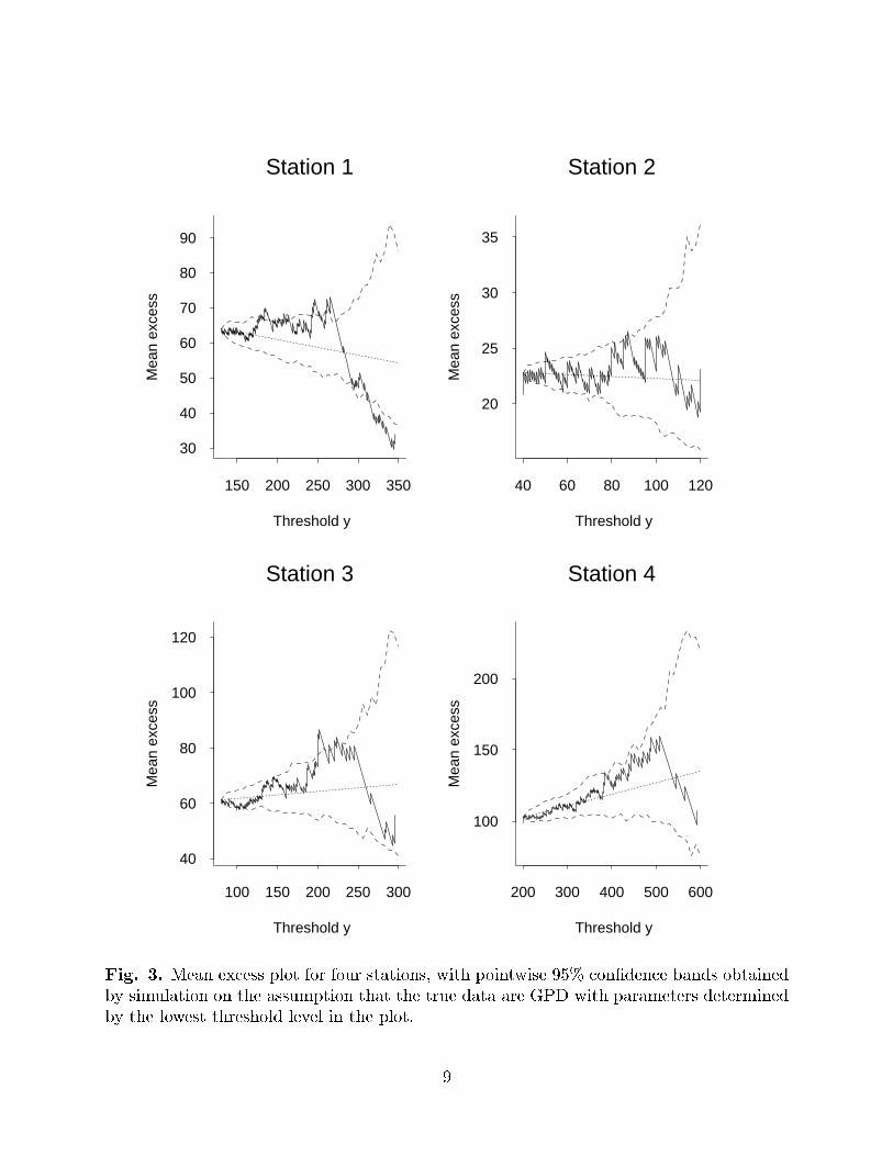
Fig. 3 shows the mean excess plot and associated con�dence bands for four stations

from the North Carolina mountains (station 1), western Colorado (2), the southern coast

of California (3) and the Atlantic coast of Florida (4). The unit of measurement is 1

100

inch, and the base threshold u has been chosen as the 98th percentile of the observed

distribution of daily rainfall values at each station. The idea of choosing the threshold

as some �xed percentile was adopted in preference to some �xed overall threshold (such

as 2 inches, cf. Karl et al. 1996) because of the enormous variability of rainfall amounts

in di�erent parts of the country, e.g. if we used a �xed threshold of 2 inches then many

western stations would have hardly any exceedances at all, making it impossible to infer

trends in the exceedance rate at those stations.

The results of this analysis are inconclusive. Three of the four plots in Fig. 3 show

apparent sharp changes of slope, but for stations 3 and 4, they occur only at high thresholds

and the plot remains within the con�dence bands except for a very short section of Figure

3. Only for station 1 does the change in slope appear statistically signi�cant. On this

basis, the threshold selection for stations 2{4 appears reasonable, but we may need to use

a higher threshold for station 1.

One disadvantage of this kind of diagnostic is that it makes no allowance for the

regression terms. In e�ect, we are assuming that the model (1) holds with constant �t, �tand �t. Alternative forms of diagnostic are based on �rst �tting a regression model and

the computing certain statistics from the �tted model.

Among these are the Z and W statistics, introduced by Smith and Shively (1995).

The Z statistics are designed to test whether intervals between exceedances are consistent

with a nonhomogeneous Poisson process. Suppose we observe (peak) exceedances at times

0 < T1 < ::: < TN < T �, and de�ne for convenience T0 = 0. Suppose the (one-dimensional)

point process of exceedance times is modeled by a nonhomogeneous Poisson process with

intensity function �(t). Then the statistics

Zk =

Z Tk

Tk�1

�(t)dt; k = 1; :::; N; (8)

should behave like independent exponential random variables with mean 1. This can be

tested in various ways, for example, using a quantile-quantile or probability plot of the order

statistics of Z1; :::; ZN against their expected values under the exponential assumption.

8

Station 1

Threshold y

Mea

n ex

cess

150 200 250 300 350

30

40

50

60

70

80

90

Station 2

Threshold y

Mea

n ex

cess

40 60 80 100 120

20

25

30

35

Station 3

Threshold y

Mea

n ex

cess

100 150 200 250 300

40

60

80

100

120

Station 4

Threshold y

Mea

n ex

cess

200 300 400 500 600

100

150

200

Fig. 3. Mean excess plot for four stations, with pointwise 95% con�dence bands obtained

by simulation on the assumption that the true data are GPD with parameters determined

by the lowest threshold level in the plot.

9

The W statistics are designed to test whether the distribution of excess values is

consistent with the model (1). Suppose we observe a high value Yt > u at time t = Tk.

Then de�ne

Wk =1

�Tklog

��Tk + �Tk(YTk � �Tk)

�Tk + �Tk(u� �Tk)

�: (9)

This is a probability integral transformation of excess values to an exponential distribu-

tion of mean 1. Hence the Wk's, like the Zk's, can be tested in various ways, including

probability plots.

Fig. 4 shows a probability plot of the Z statistics for the four stations depicted in

Fig. 3, and Fig. 5 shows the corresponding plots for the W statistics. In all cases, if the

model is a good �t, the plot should stay close to the 45o line through the origin, which is

also drawn on the plots. Of the eight plots, only the W plot for station 4 shows any real

cause for concern, an interpretation somewhat at variance with our earlier interpretation

of Fig. 3, where we suggested there was some doubt about station 1 but not about station

4. The discrepancy may be due to the fact that regression e�ects are included in Figs. 4

and 5 but not in Fig. 3.

There are other plots that may be derived from the Z and W statistics, for example

(a) plots of Zk or Wk against time Tk, as a check for hidden time trends,

(b) plots of the serial correlations of the Zk or Wk series, as a check on whether

temporal dependences have indeed been removed by the declustering which preceded this

whole analysis.

These plots are not shown here because they do not not exhibit any interesting fea-

tures.

Our overall conclusion from these diagnostics is that the models provide a reasonable

�t to the data, but there remain some questions about the appropriate choice of threshold.

In practice, we shall take account of that point primarily by conducting sensitivity tests

of our results for all 187 stations against various methods of choosing the threshold.

4. RESULTS OF SINGLE-STATION ANALYSES

The model of section 2 was �tted to each of the 187 stations, using a threshold

initially set at the 98th percentile of the empirical distribution of daily rainfall values for

each station, as in the examples discussed in section 3. Successful model �ts were obtained

for 184 stations. In the following discussion, we concentrate on the trend parameter �1,

though also giving some attention to the extreme value shape parameter �.

10

•••••••••••••••••••••••••••••••••••••••••••••••••••••••••••••••••••••••••••••••••••••••••••••••••••••••••••••••••••••••••••••••••••••••••••••••••••••••••••••••••••••••••••••••••••••••••••••••••••••••••••••••••••••••••••••••••••••••••••••••••••••••••••

••••••••••

••••• •

••

•

(Station 1)

Expected values for z

Obs

erve

d va

lues

0 1 2 3 4 5 6

0

1

2

3

4

5

•••••••••••••••••••••••••••••••••••••••••••••••••••••••••••••••••••••••••••••••••••••••••••••••••••••••••••••••••••••••••••••••••••••••••••••••••••••••••••••••••••••••••••••••••••••••••••••••••••••••••••••••••••••••••••••••••••••

••••••••••••••••••••••••••••••••••••••••••••••••••••••••••••••••••••••••••••••••••••••••••••

••••••••••••

••

••

•

(Station 2)

Expected values for z

Obs

erve

d va

lues

0 2 4 6

0

2

4

6

••••••••••••••••••••••••••••••••••••••••••••••••••••••••••••••••••••••••••••••••••••••••••••••••••••••••••••••••••••

•••••••••••••••••••••••••••••••••••••••••••••••••••••••••••••••••••••••••••••••••••••••••••••••••••••••••••••••••••••••••••••••••••••••••••••••••••••••

••••

••• •

•

•

(Station 3)

Expected values for z

Obs

erve

d va

lues

0 1 2 3 4 5 6

0

1

2

3

4

5

••••••••••••••••••••••••••••••••••••••••••••••••••••••••••••••••••••••••••••••••••••••••••••••••••••••••••••••••••••••••••••••••••••••••••••••••••••••••••••••••••••••••••••••••••••••••••••••••••••••••••••••••••••••••••••••••••••••••••••••••••••••••••••••••••••••••••••••••••••••••••••••••••••••••••••••••••••••••••••••

•••••••••••

•••••••

•••••

• ••

(Station 4)

Expected values for z

Obs

erve

d va

lues

0 2 4 6

0

1

2

3

4

5

Fig. 4. Probability plot of Z statistics based on the �tted model (4){(5) to the same four

stations as in Fig. 3.

11

•••••••••••••••••••••••••••••••••••••••••••••••••••••••••••••••••••••••••••••••••••••••••••••••••••••••••••••••••••••••••••••••••••••••••••••••••••••••••••••••••••••••••••••••••••••••••••••••••••••••••••••••••••••••••••

•••••••••••••••••••••••••••••••••••••••

••••• • •

•

•

(Station 1)

Expected values for z

Obs

erve

d va

lues

0 1 2 3 4 5 6

0

1

2

3

4

5

6

••••••••••••••••••••••••••••••••••••••••••••••••••••••••••••••••••••••••••••••••••••••••••••••••••••••••••••••••••••••••••••••••••••••••••••••••••••••••••••••••••••••••••••••••••••••••••••••••••••••••••••••••••••••••••••••••••••••••••••••••••••••••••••••••••••••••••••••••••••••••••••••••••••••••••••••••••••••••••

•••••••••••••••••••••

••••••••••• • •

•

(Station 2)

Expected values for z

Obs

erve

d va

lues

0 2 4 6

0

1

2

3

4

5

6

••••••••••••••••••••••••••••••••••••••••••••••••••••••••••••••••••••••••••••••••••••••••••••••••••••••••••••••••••••••••••••••••••••••••••••••••••••••••••••••••••••••••••••••••••••••••••••••••••••••••••••••••••••••••••••••••••••••••••••••••••••••••••••••••••••

•••••••••••••

••••••

•••

• •

•

(Station 3)

Expected values for z

Obs

erve

d va

lues

0 1 2 3 4 5 6

0

2

4

6

•••••••••••••••••••••••••••••••••••••••••••••••••••••••••••••••••••••••••••••••••••••••••••••••••••••••••••••••••••••••••••••••••••••••••••••••••••••••••••••••••••••••••••••••••••••••••••••••••••••••••••••••••••••••••••••••••••••••••••••••••••••••••••••••••••••••••••••••••••••••••••••••••••••••••••••••••••••••••

•••••••••••••••••••••

•••••••••

•••• • •

•

(Station 4)

Expected values for z

Obs

erve

d va

lues

0 2 4 6

0

1

2

3

4

5

Fig. 5. Probability plot of W statistics based on the �tted model (4){(5) to the same

four stations as in Fig. 3.

12

To aid presentation of the results, we rescale �1 in percentage terms, replacing �1 by�1100

in (5). This now has the interpretation that �1 = 1, say, corresponds to an approximate

1% per year rise in the extreme quaantiles.

The �rst point to emerge from the results is that there is enormous variability in the

estimates of �1 over the stations: from {.59 to +.68 with a mean of .063 and standard

deviation .173. Moreover, attempts to plot the spatial variability of �1 (not shown here) do

not reveal any evidence of a spatial pattern | the estimates just seem to vary arbitrarily

from one station to the next. The overall mean seems sensible | although a rise of .063%

per year might seem to be very slight, when compounded over the 87 years of the data

series, it results an overall increase of about 6% (e87�:00063 = 1:056) which is of the same

order of magnitude as the results reported by Karl and Knight (1998). Nevertheless,

the huge variability in the estimates of �1 at the individual stations causes considerable

problems for the interpretation of these results.

A similar analysis for � shows single-site estimates ranging from {.09 to +.33, with a

mean of .087 and a standard deviation of .074. In this case the evidence points towards

overall positive values of �, which is of interest because it contradicts the widely-held belief

that rainfall amounts may be modeled by a gamma distribution. For example, Stern and

Coe (1984) found the gamma distribution to be a good �t to rainfall amounts, and this was

con�rmed in an independent study by Smith (1994). In an extreme values context, � = 0

corresponds to exponential tails, which includes the gamma and many other well-known

families of distributions. � < 0 is a short-tailed case and � > 0 corresponds to a long-tailed

distribution of Pareto form. The results therefore suggest an overall tendency towards

long-tailed distributions which are not consistent with the gamma distribution.

Threshold 98% 98% 99% 99% 99.5% 99.5%

�1 � �1 � �1 �

t > 2 25 74 22 45 18 34

t > 1 73 134 58 114 61 81

t > 0 125 162 118 155 109 134

t < 0 59 22 66 29 75 50

t < �1 21 5 23 8 24 14

t < �2 10 1 5 0 5 2

Table 1. Summary table of t statistics (estimate divided by standard error) for extreme

value model applied to 187 stations and three rules for determining the threshold (top 2%,

top 1% and top 0.5%).

The second and third columns of Table 1 display the information in a di�erent way,

according to the t statistics (parameter divided by standard error) for both �1 and �.

Thus for �1, 25 out of the 184 stations have t > 2, a statistically signi�cant positive

trend according to the conventional interpretation, assuming approximate normality of

the parameter estimates. This is substantially greater than the number which would have

13

been expected by chance (.025� 184=4.6), but it still shows that the great majority of

stations, examined individually, do not have signi�cant trends. However, the number of

stations showing a positive estimate of �1, 125 out of 184, is substantially larger than would

seem plausible by chance alone, if there were no overall trend. Similar interpretations are

available for � though in this case the number of stations for which t > 2 (74) and for

which t > 0 (162) are both substantially larger than is the case for �1.

As a test of the sensitivity of these conclusions to the choice of threshold, we repeat

the analysis by replacing the 98th percentile threshold with the 99th, and then the 99.5th,

percentiles of the data at each station. For the 99th-percentile thresholds, the results are:

�1 ranges from {.78 to +.80, mean .055, standard deviation .187. � ranges from {.09 to

+.36, mean .088, standard deviation .085. For the 99.5th-percentile thresholds: �1 ranges

from {1.15 to +.81, mean .052, standard deviation .227. � ranges from {.63 to +.46, mean

.074, standard deviation .142. For both the 99% and 99.5% thresholds, the t statistics are

shown in Table 1. We conclude that for higher thresholds, the range of estimates and the

corresponding standard deviations are larger, and the tables of t statistics are consistent

with the estimates generally having larger standard errors, so depressing the individual t

statistics. There is no evidence, however, of a qualitative change in behavior as we increase

the threshold, con�rming that the precise choice of threshold does not seem unduly critical

to the analysis.

5. SPATIAL INTEGRATION

The results of section 4 appear to con�rm an overall positive trend in the extreme

daily rainfall levels, but are nevertheless hard to interpret because of the enormous spa-

tial variability. In this section, we explore ways of spatially smoothing the �1 estimates,

essentially by assuming the existence of an underlying smooth spatial �eld.

To set the problem in a slightly broader framework, suppose we are interested in a

parameter vector �(s) which we assume to vary smoothly as a function of spatial location

s lying in some domain S. Also assume that for each of a �nite subset of locations,

s 2 fs1; :::; sng, we observe a time series Y (s; t), where t is time, whose distribution dependson �(s). Suppose we have a conceptual hierarchical model of the form

(�; �) � �(�; �);

� j � � f(� j �);Y (s; �) j �; � � g(y(s; �) j �(s); �);

(10)

where the top level of the hierarchy gives a prior density for the nuisance parameters � and

�, the middle level de�nes the spatial distribution of f�(s); s 2 Sg as a function of �, and

the bottom level represents the distribution of the time series at one site s as a function

of �(s) as well as possibly additional nuisance parameters �. In principle we might allow

the time series at di�erent stations to be dependent, but this is an additional complication

14

which we shall not try to resolve here. Thus the model assumes the time series to be

independent, given � and �, from one station to another.

In the spirit of modern Bayesian approaches to hierarchical models, the model (10)

could in principle be �tted by a Markov chain Monte Carlo sampling approach. It is not

clear whether such an approach would actually be feasible for the problem under discussion,

but it would certainly be slow, and cumbersome to implement, with uncertain convergence

properties. In any case, this direct approach has not been attempted. Instead, motivated

by the preceding discussion, we propose an alternative, approximate model, for which the

computational implementation is much easier.

From the third row of model (10), we may estimate the parameter of interest, �1(s)

say (the �rst component of the vector �(s)), from the observed data at each s 2 fs1; :::; sng.Let us write the estimate as �̂1(s) and de�ne the error �(s) = �̂1(s)��1(s). Exploiting the

approximate normality of maximum likelihood estimators, assume that f�(s1); :::; �(sn)gform a multivariate normal vector with mean 0 and known covariance matrix W . Also

assume that the random �eld f�1(s); s 2 Sg is Gaussian with mean and covariance func-

tions given by a �nite-parameter model with parameter �. In particular, the mean vector

and covariance matrix of f�1(s1); :::; �1(sn)g may be written �1(�) and �1(�) respectively.

The model now becomes

�̂1(s) = �1(s) + �(s); � � N(0;W );

�1(s) � N(�1(s);�1(s));(11)

at sampling points s = s1; :::; sn. Since �(s) represents measurement error while �1(s)

re ects the inherent randomness of the environment, it is reasonable to assume that these

two components are independent. With this assumption, the two rows of (11) may be

combined to give the measurement equation

�̂1(s) � N(�1(�);�1(�) +W ) (12)

from which the parameters � may be estimated by some standard estimation procedure

such as maximum likelihood or REML. Moreover, once the parameter � is estimated, it

is then possible to reconstruct smoothed estimates of �1(s); s 2 S by kriging. The whole

procedure has much in common with standard geostatistical analysis (Cressie 1993), except

that by explicitly modeling the measurement error through the W matrix, we hope for a

more precise procedure than the standard geostatistical analysis involving a nugget e�ect.

It remains to specify parametric models for �1 and �1, and to specify the error co-

variance matrix W . In the present study, we shall assume W to be diagonal with entries

determined by the standard errors of the maximum likelihood analyses in section 4. As-

suming W to be diagonal contains an implicit assumption that the time series Y (s; �),s = s1; :::; sn, conditional on the underlying vector �eld f�(s); s 2 Sg, are independentfrom station to station. Such an assumption cannot be strictly correct, though with daily

rainfalls at relatively far away stations, it is unlikely to be too far from the truth, and in

15

any case, we do not have any straightforward means to estimate the inter-site correlations

in the procedure of sections 2{4. In a somewhat similar spatial analysis of sulfur diox-

ide trends across the eastern United States, where single-site trends had been estimated

from a generalized additive model (Hastie and Tibshirani 1990), Holland et al. (1999)

estimated the full W matrix by a bootstrapping technique, and found that taking the

o�-diagonal entries into account led to a small but not trivial change in the resulting es-

timates. Something similar remains a possibility for the present analysis, but it has not

so far been attempted. We should perhaps also note that assuming the diagonal entries

of W to be known is another simpli�cation, since the standard errors of the maximum

likelihood estimates in the analysis of section 4 are at best rough estimates of the true

standard deviations, but this is part of the price we have to pay for not pursuing a fully

Bayesian approach.

We now illustrate this method of spatial interpolation, �rst applying it to a somewhat

simpler example concerning temperature means, before returning to our main example of

rainfall extremes.

(a) Example: Mean winter daily minimum temperatures

To provide a comparative example for our study of trends in rainfall extremes, we �rst

discuss one for which the spatial modeling problem seems rather simpler. For the same

data base of 187 stations, the mean daily minimum temperature was computed for each

winter season (December, January, February), for each year from 1965 to 1996, December

being counted as part of the following year's winter. This choice of temperature variable

was motivated by recent studies suggesting that winter minimum temperatures are those

for which the strongest warming in uence is felt (see for example Easterling et al. 1997),

and the period 1965{1996 is similarly motivated by the fact that this is when the strongest

warming has been observed.

For each of 182 stations for which at least 20 years' annual winter means were available,

a mean temperature trend (in oF per year) was computed by simple linear regression. It

might be thought that time series dependence would surely be present in a series of this

form, and indeed the analysis was also carried out assuming AR(1) or AR(2) errors, but

these made very little di�erence to the results.

For the 182 temperature trends, a similar wide spatial variability was observed to that

which has already been pointed out for the rainfall extreme trends. Point estimates ranged

from {.294 to +.288 with a mean of .065 and a standard deviation of .091. After smoothing

(details to be given below), the range of temperature trends was {.035 to +.272 with a

mean of .066, standard deviation .054. Results of t tests for the individual stations, both

before and after smoothing, are given in columns 2 and 3 of Table 2. In computing this

table, the \after smoothing" estimates are based on point estimates of each �1(s) obtained

by kriging, together with a \standard error" derived from the prediction error variance.

As expected, the smoothing results in substantial shrinkage of the estimates, with much

stronger evidence of an overall positive trend | for instance, the number of stations for

16

which t > 2 increases from 37 based on unsmoothed estimates to 127 after smoothing.

Fig. 6 shows the resulting smoothed surface, represented both as a contour plot and as

a perspective plot. This shows that the strongest warming has occurred in the northern

midwest states, with much weaker trends in some other parts of the country.

Temperatures Rainfall Rainfall

98% threshold 95% threshold

1910-1996 1910-1996Before After Before After Before After

Smoothing Smoothing Smoothing Smoothing Smoothing Smoothing

t > 2 37 127 25 21 36 53

t > 1 89 157 73 80 85 154

t > 0 150 169 125 147 147 178

t < 0 32 13 59 37 36 5

t < �1 10 3 21 10 10 0

t < �2 2 0 10 3 5 0

Table 2. Summary table of t statistics for the trend parameter before and after smoothing,

on three di�erent data sets, (a) mean winter daily minimum temperatures, 1966{1996, (b)

rainfall exceedances of 98% threshold, 1910{1996, (c) rainfall exceedances of 95% threshold,

1951{1996.

The spatial smoothing method in this case assumes that �1(s), the mean of the trend

�1(s), is a cubic polynomial of the two-dimensional vector s, and the covariance matrix �1

is of the so-called Gaussian structure, with

Covf�1(si); �1(sj)g = �2 exp

��ksi � sjk2

�21

�(13)

where � = (�1; �2) are parameters to be estimated, and k � k is Euclidean distance. The

Gaussian structure of covariance function was chosen after an earlier attempt to use the

Mat�ern covariance function (equation (14) below) showed the Mat�ern shape parameter

tending to 1, which is equivalent to the Gaussian covariance function (13). The choice

of a cubic polynomial for the deterministic component of the spatial trend was made

after trying several polynomial terms and calculating the maximized log likelihoods, using

likelihood ratio tests and the AIC criterion to decide upon the cubic trend model.

(b) Application to trend estimates for rainfall extremes

The analysis of trend estimates for rainfall extremes initially follows along the same

lines as for the temperature mean trends just discussed. The estimates used here were those

reported in section 4 for the 98th percentile threshold. The spatial covariance function

between values �1(s) for di�erent s was assumed to follow a Mat�ern structure

Covf�1(si); �1(sj)g =�2

2�3�1�(�3)

�2p�3d

�1

��3

K�3

�2p�3d

�1

�(14)

17

with d = ksi � sjk, �(�) being the standard gamma function and K�3(�) a Bessel function(Handcock and Stein 1993 gave a detailed account of the Mat�ern covariance function). As

already remarked, (14) reduces to (13) as the Mat�ern shape parameter �3 tends to 1.

The units of distance d were taken to be degrees of latitude or longitude | it might be

thought that this would create diÆculties given the curvature of the earth and the fact

that one degree latitude is a bigger distance than one degree longitude, but expanding the

model by allowing a linear transformation of the plane prior to calculating d, an operation

which in the geostatistics literature is known as geometric anisotropy, did not improve

the model �t. Also, in this model the deterministic trend �1(s) was taken to be constant

since polynomial regression terms also did not improve the �t. The maximum likelihood

estimates were �̂1 = 1:42, �̂2 = :012, �̂3 = 0:30. Thus the critical range parameter �̂1 is very

small compared with the total spatial range of the data, and the value of �̂3 also indicates

a spatial covariance function which is nearly discontinuous at 0. These estimates should

lead us to expect a rather rough �tted surface and this expectation is amply con�rmed by

the contour and perspective plots shown in Fig. 7. The smoothed estimates of �1 range

from {.22 to +.24 with a mean of .061, standard deviation .082, and the t-statistics after

smoothing are shown in columns 4 and 5 of Table 2. The number of estimates for which

t > 0 is increased compared with Table 1, but those for which t > 2 are decreased, and

overall it is questionable whether the attempt to smoothe the trend estimates has been

successful.

(c) Improving the trend estimates for rainfall extremes

The unsatisfactory results so far point towards the need for a di�erent approach.

One possible source of diÆculty (suggested by Ian Jolli�e) is that since we are restricting

attention to very extreme events, we could not expect much spatial coherence | maybe

we would do better with a lower set of thresholds. Another possible source of diÆculty is

due to missing data | although we have assumed a linear trend in (5), we have no reason

to believe that this is necessarily correct, and if we compared the �tted linear trend at

two stations with very di�erent periods of data, we could be in diÆculties because the real

trends are di�erent over the respective periods.

In an attempt to reduce these diÆculties, the extreme value analysis was repeated for

thresholds de�ned by the 95th percentile at each station, and with all analyses restricted

to the period 1951{1996 for which relatively complete data records are available. The

model was successfully �tted to 183 stations, with estimates of �1 which ranged from {.33

to +.62, mean .099, standard deviation .130. The Mat�ern model (14) now resulted in

parameter estimates �̂1 = :0045, �̂2 = 2:80, �̂3 = :022, and smoothed �1 estimates ranging

from {.036 to +.185, mean .090, standard deviation .039. Already there is much clearer

evidence of shrinkage. The t statistics, both before and after smoothing, are shown in

columns 6 and 7 of Table 2, and the contour and perspective plots of the smoothed surface

are shown in Fig. 8. The resulting surface is still not nearly as smooth as it was for the

temperature mean trends, but it is much smoother than in the earlier analysis of rainfall

extreme trends. With 178 out of 183 stations now showing a positive smoothed trend, the

evidence that the overall trend really is positive is overwhelming.

18

-0.

0

00.1

0.1

0.2

0.2

0.3

0.30.4

4060

80100

2

40

60

80

100

Y

-0.2-

0.1

00.

10.

20.

30.

40.

5Z

Fig. 6. Contour and perspective plots for the reconstructed trend surface based on means

of daily mean winter temperatures, 1966-1996.

19

-0.1-0.09

-0.09-0.08

-0.08-0.07

-0.07-0.06

-0.06-0.05

-0.05

-0.05-0.04

-0.04

-0.04-0.03

-0.03

-0.03

-0.02

-0.02

-0.02

-0.02 -0.02

-0.02

-0.01

-0.01

-0.01-0.01 -0.01

-0.01

0

0

0

0 0

0

0

0

0.01

0.01

0.01

0.010.01

0.01

0.01

0.01

0.01

0.02

0.02

0.02

0.02

0.02

0.02

0.020.02 0.02

0.02

0.020.03

0.03 0.03

0.030.03 0.030.03

0.03

0.03

0.030.04

0.04

0.04

0.04

0.040.04

0.04

0.04

0.04

0.040.04

0.04 0.04

0.04

0.04

0.05

0.05 0.05

0.05

0.05

0.05

0.05

0.05

0.05

0.05

0.06

0.06

0.06 0.06

0.06

0.06

0.06

0.06

0.0

0.07

0.070.07

0.07

0.07 0.07

0.070.07

0.07 0.07

0.0

0.08

0.08

0.08

0.08

0.080.08

0.08

0.08

0.08

0.08

0.08

0.08 0.08

0.08

0.08

0.08

0.08 0.08

0.08

0.09

0.09

0.09

0.09

0.09

0.09

0.09

0.09

0.09

0.09

0.09

0.09

0.09

0.09

0.09

0.09

0.09

0.1

0.1

0.1

0.1

0.1

0.1

0.1

0.1

0.1

0.1

0.1

0.1

0.1

0.10.1

0.1 0.10.11

0.11

0.11

0.11

0.110.11

0.11

0.11

0.11

0.11

0.110.11

0.11 0.11

0.12

0.12

0.12

0.120.12

0.12

0.12

0.12

0.120.12

0.12

0.13

0.13

0.13

0.13

0.13

0.13

0.14

0.14

0.150.16

4060

80100

X20

40

60

80

100

Y

-0.1

5-0.1-

0.05

00.

050.

10.1

50.2

Z

Fig. 7. Contour and perspective plots for the reconstructed trend surface based on

precipitation exceedances above the 98% threshold, 1910{1996.

20

0.0740.076

0.076

0.0780.078

0.078

0.078

0.078

0.08

0.08

0.082

0.082

0.082

0.082

0.084

0.084 0.084

0.084

0.086

0.086

0.086

0.0860.086

0.08

0.0860.086

0.088

0.088

0.088

0.088

0.0880.09

0.09

0.09

0.09

0.092

0.092

0.092

0.0920.092

0.094 0.094

0.094

0.096

0.098

0.098

0.10.102

0.102

0.104

0.104

0.106

0.106

0.106

0.1060.108

0.1080.11

4060

80100

X20

40

60

80

100

Y

0.04

0.06

0.08

0.1

0.12

Z

Fig. 8. Contour and perspective plots for the reconstructed trend surface based on

precipitation exceedances above the 95% threshold, 1951{1996.

21

6. REGIONAL AVERAGES

One application of the spatial integration procedure is to the calculation of regional

averages. Part of the reason for doing this is that while the reconstruction of the trend at

a single site is still problematic, a much clearer picture of the results emerges if we look at

regional averages.

Suppose we are interested in estimating

V (R) =

ZR

�1(s)ds; (15)

where �1(s) is the site-speci�c trend at s and R � S is some region of space. If we denote

by ~�1(s) the smoothed spatial estimates at site s, then a natural estimate of V (R) is

~V (R) =

ZR

~�1(s)ds; (16)

and we also have

Ef~V (R)� V (R)g2 =ZR

ZR

Ehf~�1(s1)� �1(s1)gf~�1(s2)� �1(s2)g

ids1ds2; (17)

there is a standard formula from kriging theory for the covariance between predictions

at two sites (cf. Cressie 1993, pp. 154{155), and this may be substituted into (17) to

obtain an approximate standard error for ~V (R). In practice, the integrals in (16) and

(17) are replaced by sums over a suitable dense grid. The standard error formula is only

approximate because the prediction error variance formula on which it is based ignores

the component of variability due to parameter estimation; in practice, therefore, we might

expect the standard errors which follow from (17) to underestimate the true variability of

the estimates.

To apply these methods, the continental U.S.A. was divided into several subregions

(Fig. 9), with A, B, C and D representing reprectively the north-west, north-east, south-

west and south-east quarters of the country. A region E was also identi�ed, corresponding

to the northern midwest region for which we saw in section 5 that the warming in temper-

ature means is greatest. The choice of regions is not intended to have any signi�cance in

itself but merely to illustrate how the estimates vary over di�erent regions.

Table 3 shows estimates of the mean trend and standard errors for the regions A{E and

for the country overall, applying the formulae (16){(17) to the smoothed point estimates

from sections 5(a) for the temperature means and 5(c) for the rainfall extremes. Although

the same spatial methodology has been applied in both cases, it can now be seen that the

results are very di�erent.

22

A B

C D

E

Fig. 9. Outline of regions used for regional trend calculation. Regions A,B,C,D refer

respectively to the north-west, north-east, south-west and south-east quadrants, bounded

by the solid lines. Region E is the northern midwest region, bounded from east and west

by the dotted lines and from the south by the central solid line.

Region Mean (S.E.) Rainfall (S.E.)

Temperatures Extremes

Trend Trend

A .105 (.011) .091 (.011)

B .131 (.020) .087 (.011)

C .091 (.031) .096 (.013)

D .009 (.029) .088 (.012)

E .170 (.017) .094 (.010)

All .086 (.012) .090 (.009)

Table 3. Regionally averaged trends and standard errors for �ve regions of USA, and

overall. Trends shown are for temperature means data (cols. 2 and 3) and for rainfall

extremes data based on 95% threshold, 1951{1996 (col2. 4 and 5).

For the temperature trends, we indeed see a strong positive trend in region E and

less strong but still signi�cant trends in each of A, B and C; however, for region D, there

appears to be no trend at all. As judged by the standard errors, these di�erences are clearly

23

statistically signi�cant. In contrast, for the trends in rainfall extremes, the regionally

averaged trend estimates are very consistent, being about .09 for all the regions.

The interpretation of our earlier results is now much clearer. For the mean temperature

trends, there are clear di�erences between di�erent parts of the country and these are

re ected in the regional estimates. In contrast, for trends in the rainfall extremes, there is

very little spatial structure at all: the mean estimated trend is about .09 everywhere, and

the varability about this level, which we saw in Fig. 8, appears to be just local random

variation.

7. CONCLUSIONS

The �nal results of our study of rainfall extremes are based on all exceedances of

the 95th percentile threshold at each station, and for all years from 1951{1996 for which

reasonably complete records are available. The results show an upward trend in extreme

quantiles of about 0.09% per year. Noting that e46�:0009 = 1:042, this amounts to about

a 4% overall rise in extreme daily rainfall levels over that period.

Karl and Knight (1998) also found an overall positive trend in the top 5% of the data,

but when they repeated the analysis across various subregions, they found considerable

regional di�erences. In contrast, the most striking feature of the present results, especially

when they are contrasted with the results for mean temperatures, is that they are remark-

ably consistent over di�erent regions. No immediate explanation suggests itself as to why

the current results are di�erent from Karl and Knight in this respect, but as noted at the

beginning of the paper, it is diÆcult to see how one would quantify the sampling variability

in the Karl-Knight technique, whereas for the present approach, based on speci�c models,

this is easier.

Another feature of the present approach is that it could quite easily be adapted to

compute di�erent functionals of the extreme rainfall distribution, for example, di�erent

measures of extremal behavior at a single site or di�erent spatial aggregations.

There remain many open questions, both statistical and climatological. From the

statistical point of view, the spatial smoothing technique has involved a number of sim-

plifying assumptions, such as assuming that the single-site estimates in (11) are normally

distributed, assuming the W matrix is known and diagonal, and ignoring the e�ect of

parameter estimation in computing the standard errors of regional averages, in (17). In

principle, all of these diÆculties could be avoided if we adopted a fully Bayesian approach

to the model (10), but the computational e�ort required for the present results was con-

siderable, and a fully Bayesian computation does not seem feasible at the present time.

Another statistical point for further discussion is the possibility of looking at more

complicated trends than linear trends, in (5). At the start of this analysis, it seemed very

unclear whether any overall trend would be found, and this was part of the reason for

24

restricting attention to a simple linear trend. Since our �nal conclusion is that such a

trend does exist, however, the logical next step would be to consider how the trend varies

over di�erent time periods.

From a climatological point of view, it needs to be emphasized that our results are

primarily descriptive: they provide empirical evidence of the existence of a trend, but they

do not give any insight into the causes of that trend. Nevertheless, as remarked at the

beginning of the paper, it is of considerable interest to determine whether observed climatic

trends are consistent with the projections of numerical climate models under various forcing

factors including both anthropogenic and natural components. Such a study was initiated

by Karl et al. (1996) for the climatic indicators in their paper; it would be of considerable

interest to continue the study of climate model data using the statistical methods of the

present paper.

REFERENCES

Cressie, N. (1993), Statistics for Spatial Data. Second edition, John Wiley, New York.

Davison, A.C. and Smith, R.L. (1990), Models for exceedances over high thresholds

(with discussion). J.R. Statist. Soc., 52, 393-442.

Easterling, D.R., Horton, B., Jones, P.D., Peterson, T.C., Karl, T.R., Parker, D.E.,

Salinger, M.J., Razuvayev, V., Plummer, N., Jamason, P. and Folland, C.K. (1997), Max-

imum and minimum temperature trends for the globe. Science 277, 364{367.

Hall, P. and Weissman, I. (1997), On the estimation of extreme tail probabilities.

Annals of Statistics 25, 1311{1326.

Handcock, M.S. and Stein, M. (1993), A Bayesian analysis of kriging. Technometrics,

35, 403-410.

Hastie, T.J. and Tibshirani, R.J. (1990), Generalized Additive Models. Chapman and

Hall, London.

Holland, D.M., De Oliveira, V., Cox, L.H. and Smith, R.L. (1999), Estimation of

regional trends in silfur dioxide over the Eastern United States. Preprint, Environmental

Protection Agency and National Institute of Statistical Sciences, Research Triangle Park,

North Carolina.

Karl, T.R. and Knight, R.W. (1998), Secular trends of precipitation amount, fre-

quency, and intensity in the USA. Bull. Amer. Meteor. Soc. 79, 231{241.

Karl, T.R., Knight, R.W., Easterling, D.R. and Quayle, R.G. (1996), Indices of climate

change for the United States. Bull. Amer. Meteor. Soc. 77, 279{292.

Leadbetter, M.R., Lindgren, G. and Rootz�en, H. (1983), Extremes and Related Prop-

erties of Random Sequences and Series. Springer Verlag, New York.

Ledford, A.W. and Tawn, J.A. (1998), Diagnostics for dependence within time-series

extremes. Preprint, University of Surrey.

Smith, R.L. (1989), Extreme value analysis of environmental time series: An appli-

cation to trend detection in ground-level ozone (with discussion). Statistical Science 4,

367-393.

25

Smith, R.L. (1994), Spatial modelling of rainfall data. In Statistics for the Envi-

ronment, Volume 2 (V. Barnett & F. Turkman, editors), pp. 19-41. Chichester: John

Wiley.

Smith, R.L. and Shively, T.S. (1995), A point process approach to modeling trends in

tropospheric ozone Atmospheric Environment 29, 3489{3499.

Smith, R.L., Tawn, J.A. and Coles, S.G. (1997), Markov chain models for threshold

exceedances. Biometrika 84, 249{268.

Stern, R.D. and Coe, R. (1984), A model �tting analysis of daily rainfall data (with

discussion). J.R. Statist. Soc. A 147, 1-34.

Wigley, T.M.L., Smith, R.L. and Santer, B.D. (1998), Anthropogenic in uence on the

autocorrelation structure of hemispheric-mean temperatures. Science. November 27 1998.

26