1

Q u a lita tiveM eth od

U n ivaria teD ata

A n a lys is

Q u an tita tiveM eth od s

In te llig en ceP h ase

U n d ers tan d in gth e R e la tion s

M od e lin g th eP rob lem

B iiva ria te o rM u ltiva ria te

D ataA n a lys is

D es ig nP h ase

C h o ice P h ase

D ec is ionS c ien ce

F ou n d ation s

The Design Phase

2

What Is A Model?

• A model is a representation or abstraction of a real-world object, process, concept or “problem” which is reduced in scope or complexity relative to the problem itself but yet retains the certain “essential” aspects which we believe define or characterize the particular real-world problem.

•A good model should have a good balance between accuracy and simplicity.

3

What Is A Model?

• A models may be used to:•describe

•predict, or

•optimize

• Three types of general models

• Physical/iconic: model car, model house• Analog/graphic: road map, speedometer• Symbolic: algebraic or spreadsheet model

4

Why Use Models?

In support of Decision Making and help management make sound decisions

A model is valuable if you make better decisions when you use it (modeling approach) than when you don’t (intuition approach)

Models + Managerial Judgement = The best way to run business

5

Advantages of Using Models

Models are generally less expensive and disruptive than experimenting with real systems

Models allow managers to ask “what-if” questions

Models force a consistent and systematic approach to the analysis of problems

6

Advantages of Using Models

“By modeling various alternatives for future system design, Federal Express has, in effect, made its mistakes on paper. Computer modeling works; it allows us to examine many different alternatives and it forces the examination of the entire problem”

Fred Smith

Chairman and CEO of FedEx

7

Disadvantages of Models

They may be expensive and time-consuming to develop and test

They are often misused and misunderstood because of their mathematical complexity

They may have assumptions that oversimplify the real-world system

8

Model Components

Model- Relationships

Inputs Outputs

9

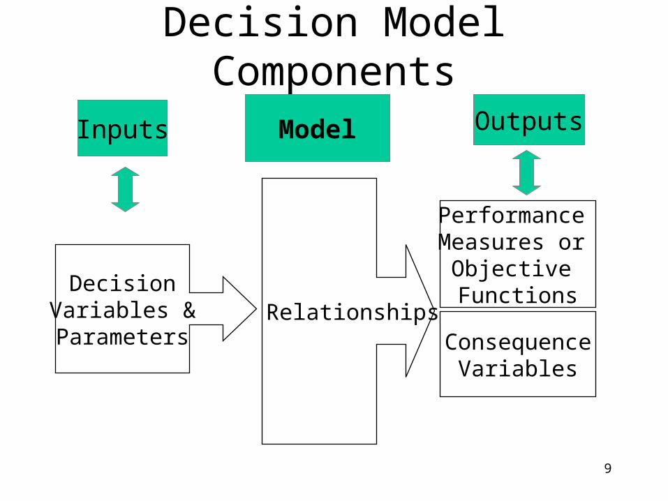
Decision Model Components

DecisionVariables &Parameters

Relationships

Performance Measures or

Objective Functions

ConsequenceVariables

Inputs OutputsModel

10

Model and Data

Useful (quantitative) models are developed based on relevant data (numbers); models without data are at best theoretical abstractions

Data are often collected according to the requirements of models– time series vs. cross-sectional– aggregated vs. disaggregated

11

Numbers in Models

Data– Count– Measure– Rank

Results

Constant Variable Coefficient Precision

12

Model Classification

Deterministic Models– All model components and relevant data are

known with certainty• Examples include: Ad hoc models, Forecasting,

Decision analysis, Constrained optimization

Probabilistic (Stochastic) Models– Some components or data are not known with

certainty• Examples of include: Monte Carlo simulation,

Scheduling and queueing

13

General Modeling Process

Diagnose problem Organize facts Select methodology Formulate model Solve model Interpret results

Validate– Face validity

– Causal validity

– Computational validity

Sensitivity analysis

Implement solution

Monitor results

14

Abstract aspect of real problem

Real World Problem

Model

Is the model valid?

Study model behavior

Make decisions

Monitor resultsModel solution

No Yes

Basic Modeling Process

15

Fundamental Relationships

Accounting

Microeconomics

Logic

16

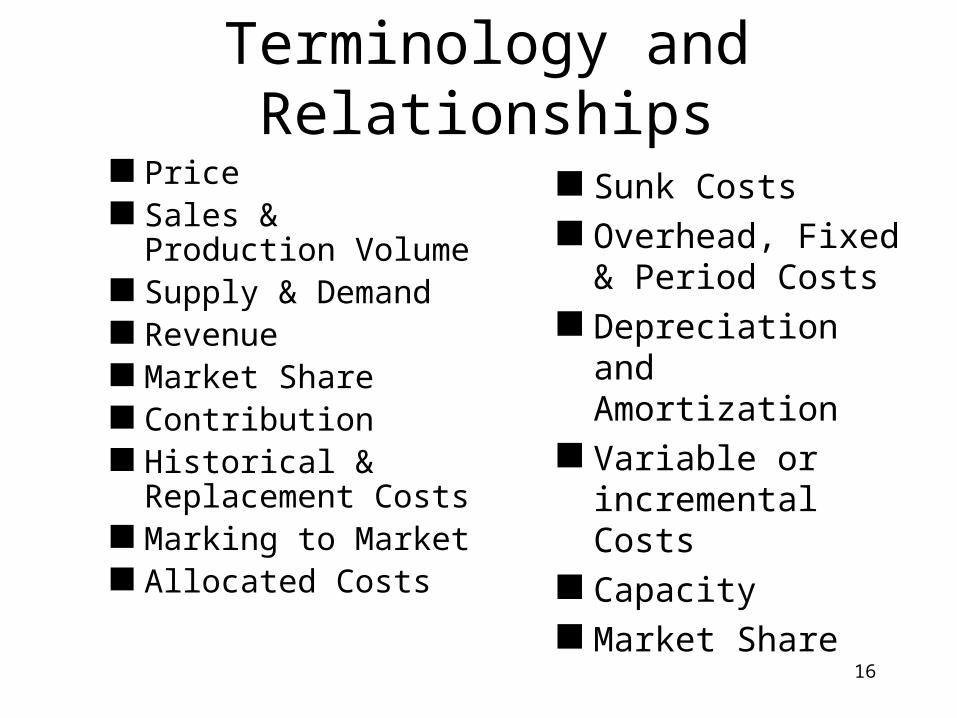
Terminology and Relationships

Price Sales & Production

Volume Supply & Demand Revenue Market Share Contribution Historical &

Replacement Costs Marking to Market Allocated Costs

Sunk Costs Overhead, Fixed &

Period Costs Depreciation and

Amortization Variable or

incremental Costs Capacity Market Share

17

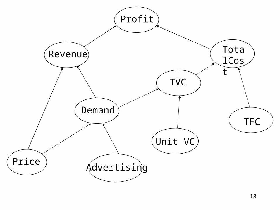
Model Building: Influence Diagram

A graphical representation (flow chart) of

the influencing relationship among

variables in a particular problem

Constructing an influence diagram using Top-Down approach – start with output: performance measure– work downward to locate variables that affect

the output as well as other variables

18

Profit

TotalCost

Revenue

Price

Demand

TVC

TFC

Unit VC

Advertising

19

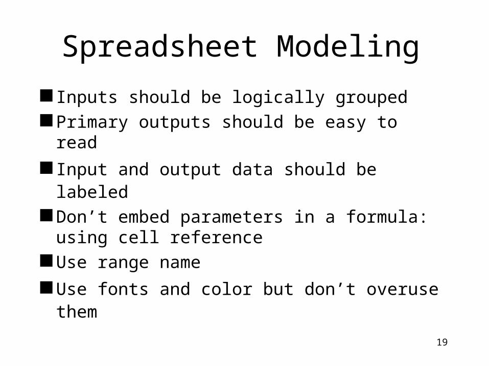
Spreadsheet Modeling

Inputs should be logically grouped Primary outputs should be easy to read

Input and output data should be labeled Don’t embed parameters in a formula: using

cell reference Use range name

Use fonts and color but don’t overuse them

20

O utput o r H istorica lVa lid ity

R e la tionsh ip Va lid ity

Face Va lid ity

Va lida te M ode l

Bu ild M ode l

D iagnosis

21

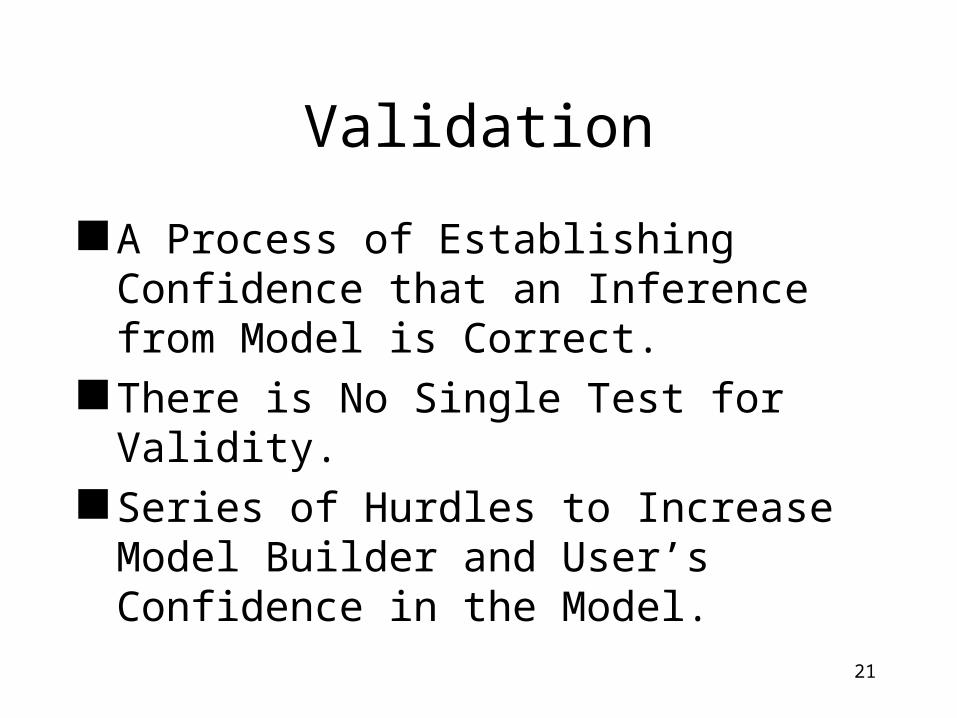
Validation

A Process of Establishing Confidence that an Inference from Model is Correct.

There is No Single Test for Validity. Series of Hurdles to Increase Model Builder

and User’s Confidence in the Model.

22

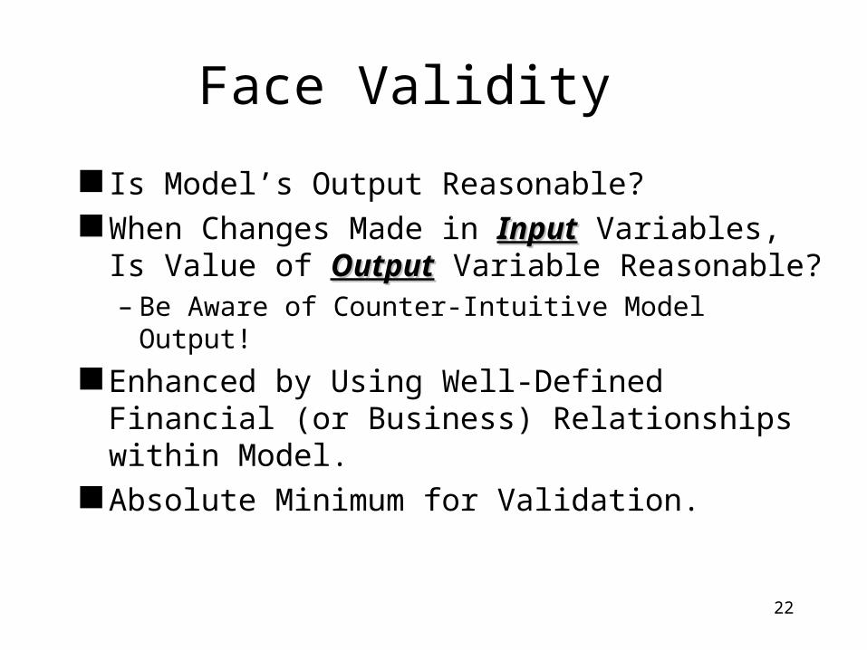
Face Validity

Is Model’s Output Reasonable? When Changes Made in InputInput Variables, Is

Value of OutputOutput Variable Reasonable?– Be Aware of Counter-Intuitive Model Output!

Enhanced by Using Well-Defined Financial (or Business) Relationships within Model.

Absolute Minimum for Validation.

23

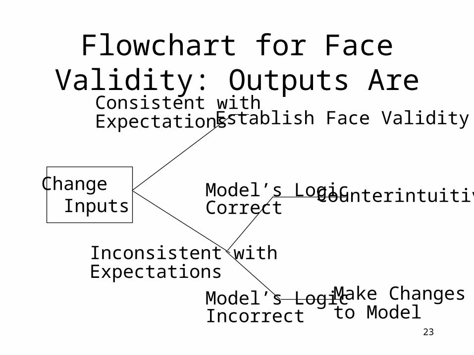
Flowchart for Face Validity: Outputs Are

Change Inputs

Consistent withExpectations Establish Face Validity

Inconsistent withExpectations

Model’s LogicCorrect

Counterintuitive

Model’s LogicIncorrect

Make Changesto Model

24

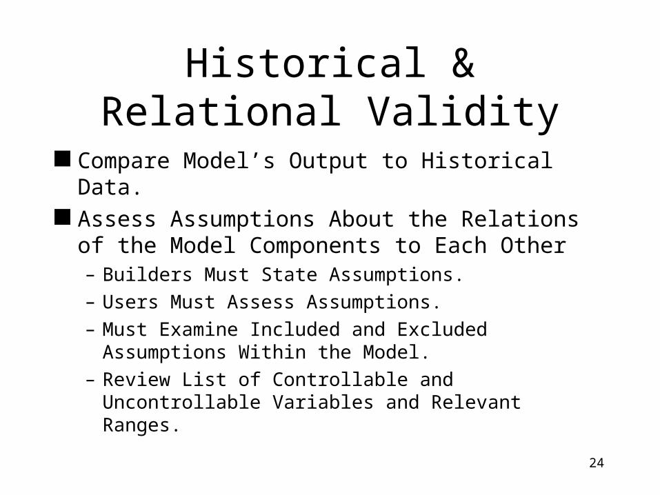
Historical & Relational Validity

Compare Model’s Output to Historical Data. Assess Assumptions About the Relations of the

Model Components to Each Other– Builders Must State Assumptions.

– Users Must Assess Assumptions.

– Must Examine Included and Excluded Assumptions Within the Model.

– Review List of Controllable and Uncontrollable Variables and Relevant Ranges.

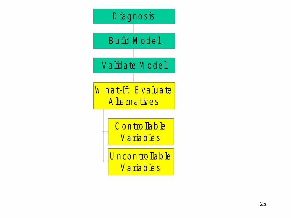
25

C ontro llab leVariab les

U ncontro llab leVariab les

W hat-If: Eva lua teA lte rna tives

Va lida te M ode l

Bu ild M ode l

D iagnosis

26

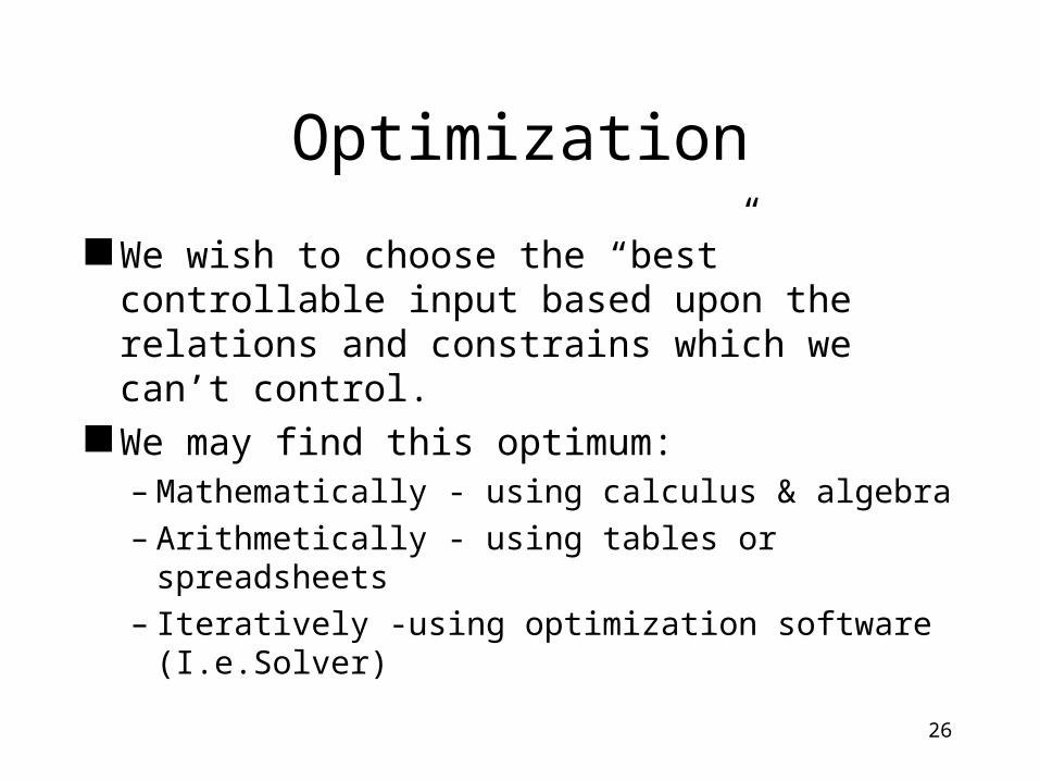
Optimization

We wish to choose the “best” controllable input based upon the relations and constrains which we can’t control.

We may find this optimum:– Mathematically - using calculus & algebra– Arithmetically - using tables or spreadsheets– Iteratively -using optimization software

(I.e.Solver)

27

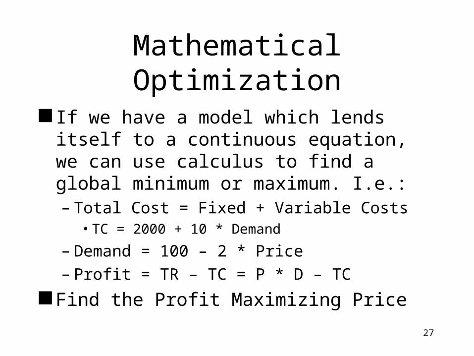
Mathematical Optimization

If we have a model which lends itself to a continuous equation, we can use calculus to find a global minimum or maximum. I.e.:– Total Cost = Fixed + Variable Costs

• TC = 2000 + 10 * Demand

– Demand = 100 – 2 * Price– Profit = TR – TC = P * D – TC

Find the Profit Maximizing Price

28

Arithmetical Optimization

If we don’t have a differentiable equation or a continuous relation but do have a simple equation, we may find an optimum arithmetically using one way or two way tables or spreadsheets.

29

One-Way What-If Table

Order Size Total Annual Cost

6000

5000

4000

3000

2000

1000

500

30

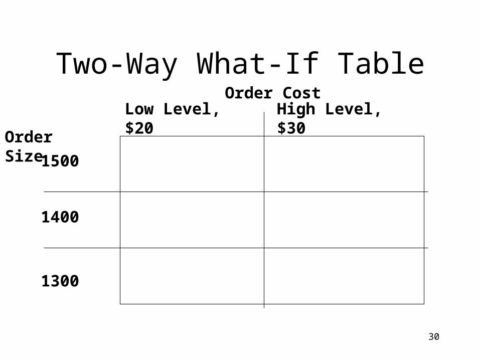
Two-Way What-If Table

Low Level, $20 High Level, $30

1500

Order Size

Order Cost

1300

1400

31

Iterative Optimization

If we have several controllable variables and/or the variables can take on many different values, we may find an optimum using software which iteratively applies numerical methods such as Excel’s Solver.

Since this is numerical (and not mathematical), we cannot be assured that we have found a truly global optimum but instead may have found a local one.

32

Hill Climbing

33

Using Excel’s Solver for Optimization

Answers Questions Such As:– What Order Size Will Minimize Total Annual

Cost?– How Much Should I Invest in Stock 1 to

Maximize Portfolio Return?

OutputOutput (AKA TargetTarget) Cell is Cell Whose Value You Wish to Maximize or Minimize.

34

Using Excel’s Solver

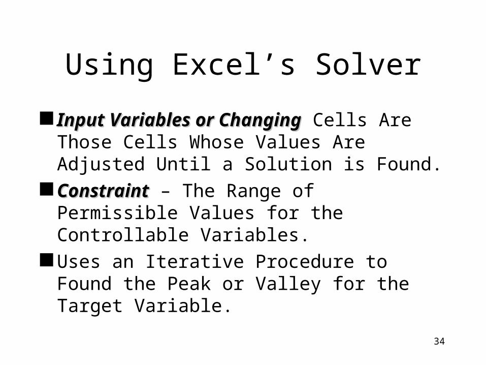
Input Variables or ChangingInput Variables or Changing Cells Are Those Cells Whose Values Are Adjusted Until a Solution is Found.

ConstraintConstraint – The Range of Permissible Values for the Controllable Variables.

Uses an Iterative Procedure to Found the Peak or Valley for the Target Variable.

35

Optimization Using Solver

36

Problem Using Excel’s Solver

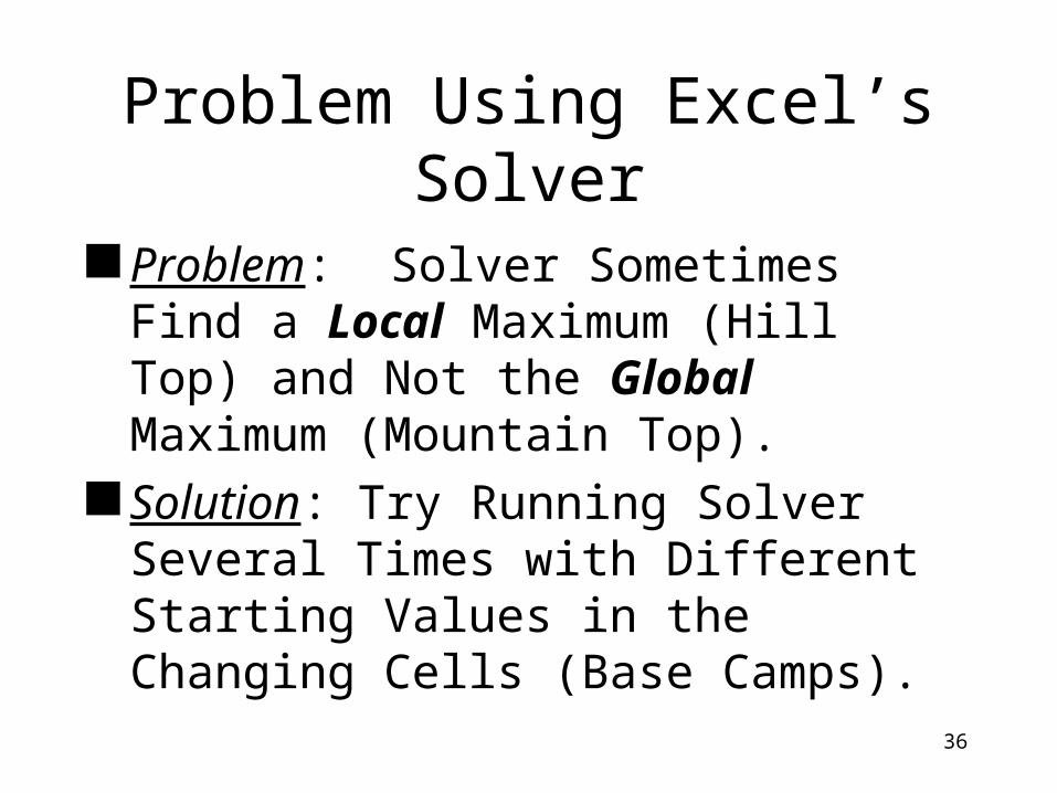
Problem: Solver Sometimes Find a Local Maximum (Hill Top) and Not the Global Maximum (Mountain Top).

Solution: Try Running Solver Several Times with Different Starting Values in the Changing Cells (Base Camps).

37

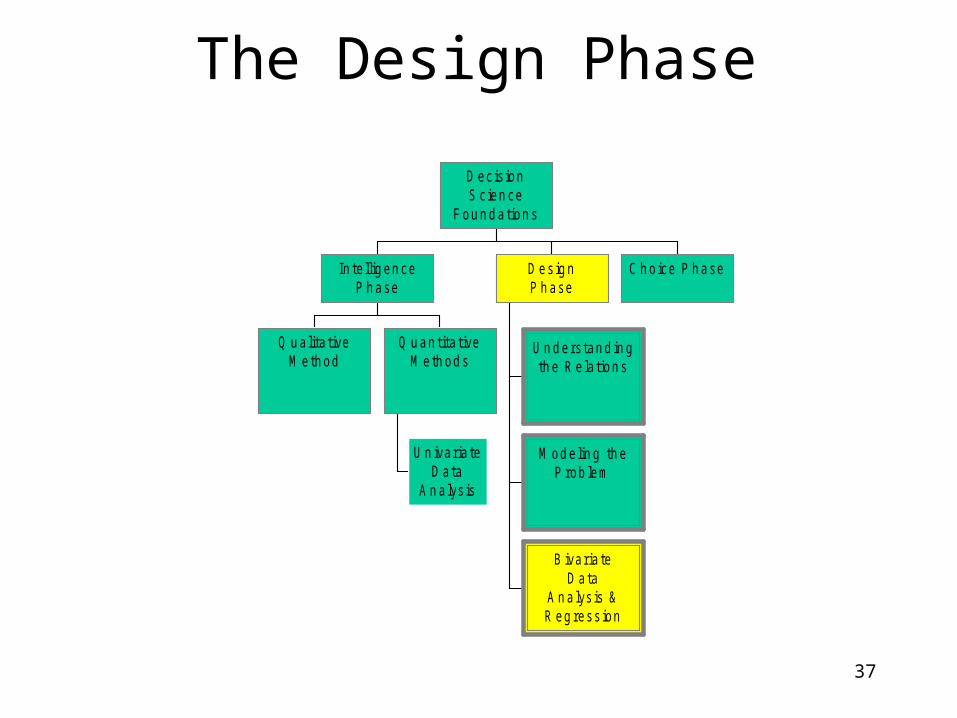
Q u a lita tiveM eth od

U n ivaria teD ata

A n a lys is

Q u an tita tiveM eth od s

In te llig en ceP h ase

U n d ers tan d in gth e R e la tion s

M od e lin g th eP rob lem

B ivaria teD ata

A n a lys is &R eg ress ion

D es ig nP h ase

C h o ice P h ase

D ec is ionS c ien ce

F ou n d ation s

The Design Phase

38

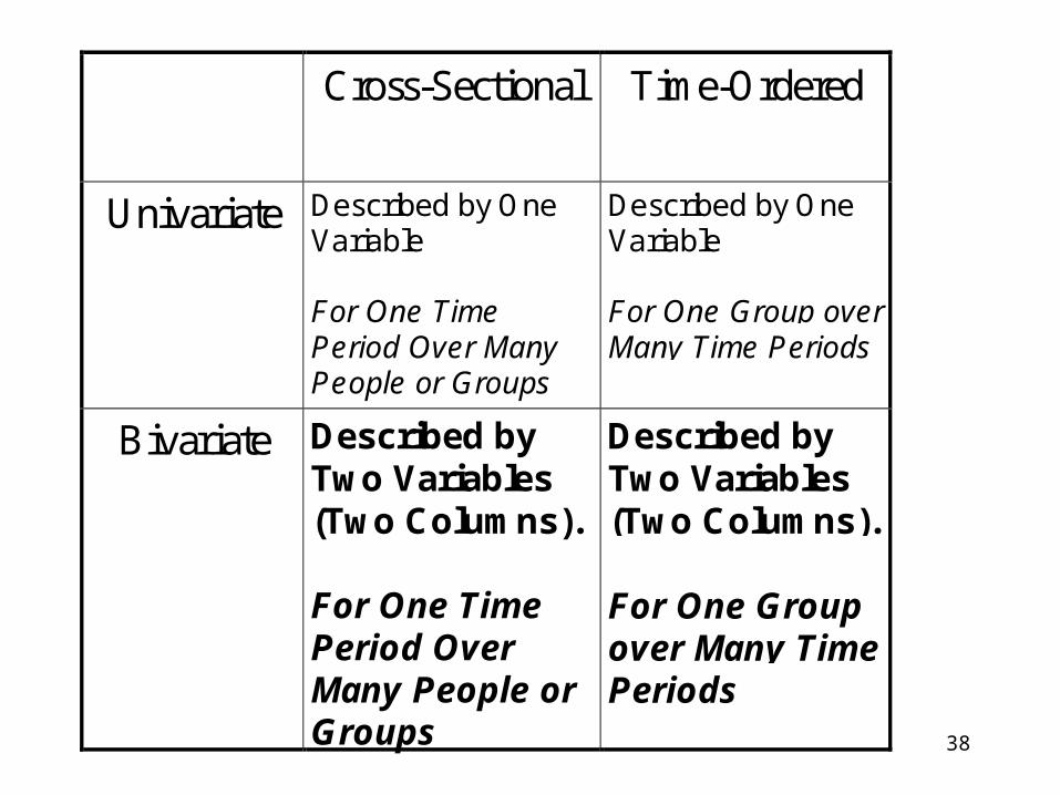
Cross-Sectional Time-Ordered

Univariate Described by OneVariable

For One TimePeriod Over ManyPeople or Groups

Described by OneVariable

For One Group overMany Time Periods

Bivariate Described byTwo Variables(Two Columns).

For One TimePeriod OverMany People orGroups

Described byTwo Variables(Two Columns).

For One Groupover Many TimePeriods

39

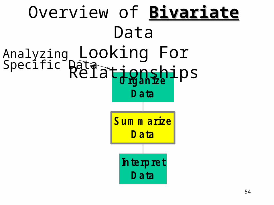
InterpretD ata

Sum m arizeD ata

OrganizeD ata

Overview of BivariateBivariate Data: Looking For Relationships

AnalyzingSpecific Data

40

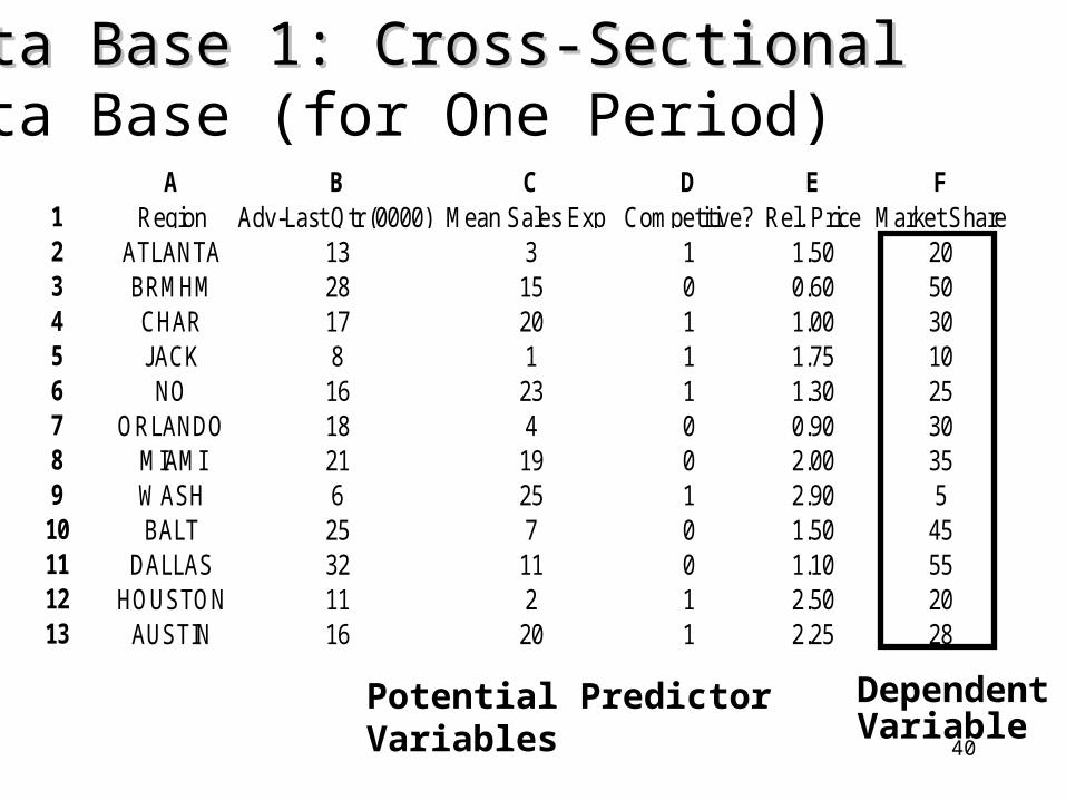
Data Base 1: Cross-SectionalData Base 1: Cross-Sectional Data Base (for One Period)

A B C D E F1 Region Adv-Last Qtr (0000) Mean Sales Exp Competitive? Rel. Price Market Share2 ATLANTA 13 3 1 1.50 203 BRMHM 28 15 0 0.60 504 CHAR 17 20 1 1.00 305 JACK 8 1 1 1.75 106 NO 16 23 1 1.30 257 ORLANDO 18 4 0 0.90 308 MIAMI 21 19 0 2.00 359 WASH 6 25 1 2.90 510 BALT 25 7 0 1.50 4511 DALLAS 32 11 0 1.10 5512 HOUSTON 11 2 1 2.50 2013 AUSTIN 16 20 1 2.25 28

DependentVariable

Potential Predictor Variables

41

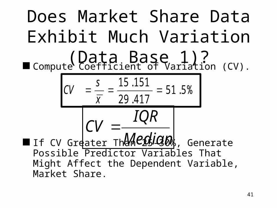
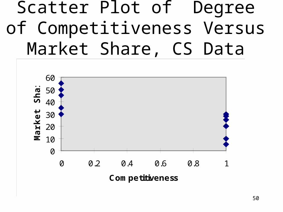
Does Market Share Data Exhibit Much Variation (Data Base 1)?

Compute Coefficient of Variation (CV).

If CV Greater Than 25-30%, Generate Possible Predictor Variables That Might Affect the Dependent Variable, Market Share.

%..

.551

41729

15115

x

sCV

Median

IQRCV

42

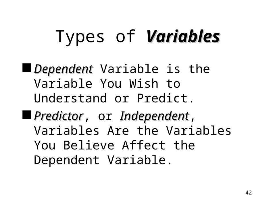
Types of VariablesVariables

DependentDependent Variable is the Variable You Wish to Understand or Predict.

PredictorPredictor, or IndependentIndependent, Variables Are the Variables You Believe Affect the Dependent Variable.

43

Correlation

If two variables are related to each other, then changes in one can be related to changes in the other. In other words, they rise and/or fall together.

Measured by a coefficient -1 r 1 One variable may be caused by the other

OR they both may be caused by other causes (intervening variables).

44

Causal Models

Causal Models - where we have one numerical dependent variable and one or more independent variables which we say “cause” the dependent variable– Salary is “caused by” gender and months on the

job.– Wrecks are “caused by” alcohol, cell phones,

speed, etc.– Advertising “causes” sales.

45

Establishing Causality

Necessary (but not sufficient) determinates of Causality:– Correlation - variables rise and/or fall together.– Temporal precedence - cause precedes effect in

time.– Logical mechanism - must have reasonable

explanation of how independent variable causes the dependent variable to vary.

46

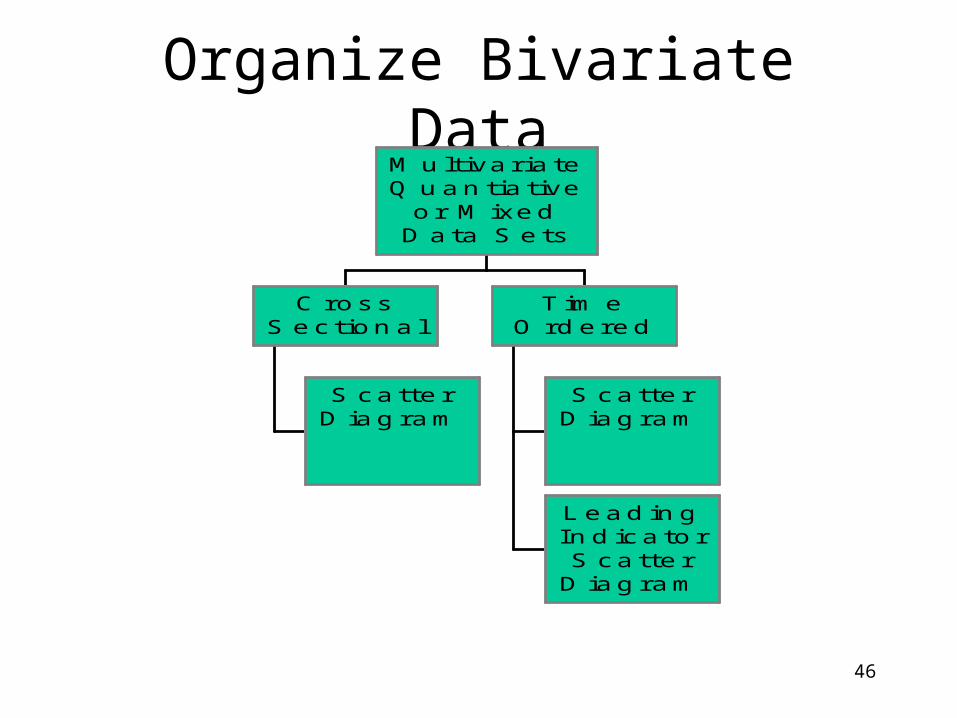
Organize Bivariate Data

S catte rD iag ram

C rossS ec tion a l

S ca tte rD iag ram

L ead in gIn d ica to rS ca tte r

D iag ram

Tim eO rd ered

M u ltiva ria teQ u an tia t ive

or M ixedD ata S e ts

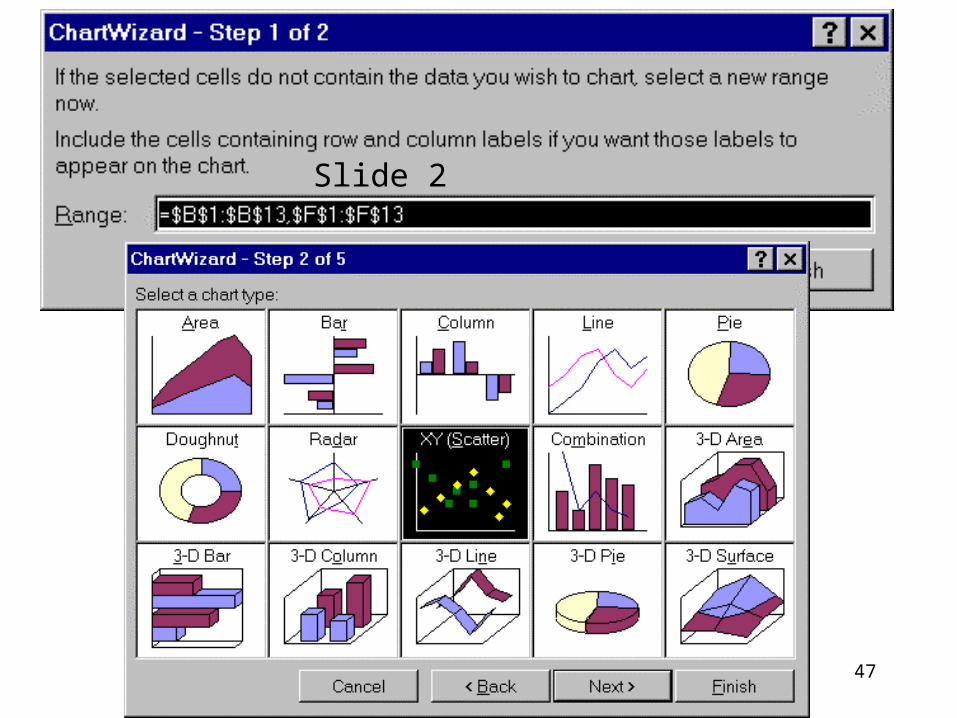
47

Slide 2

48

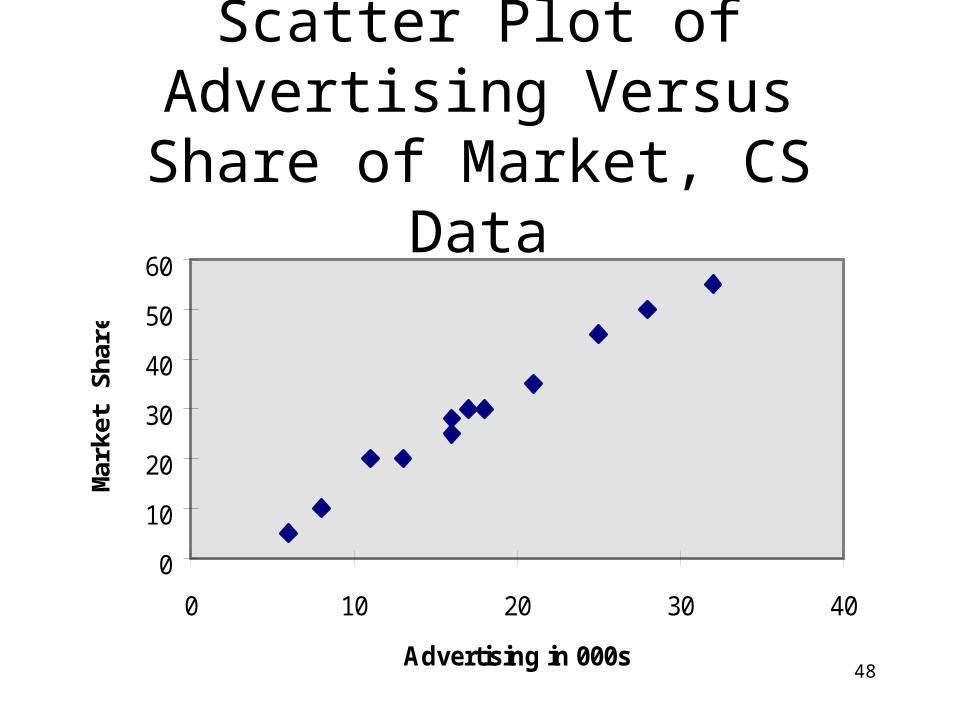
Scatter Plot of Advertising Versus Share of Market, CS Data

0

10

20

30

40

50

60

0 10 20 30 40

Advertising in 000s

Mar

ket S

hare

49

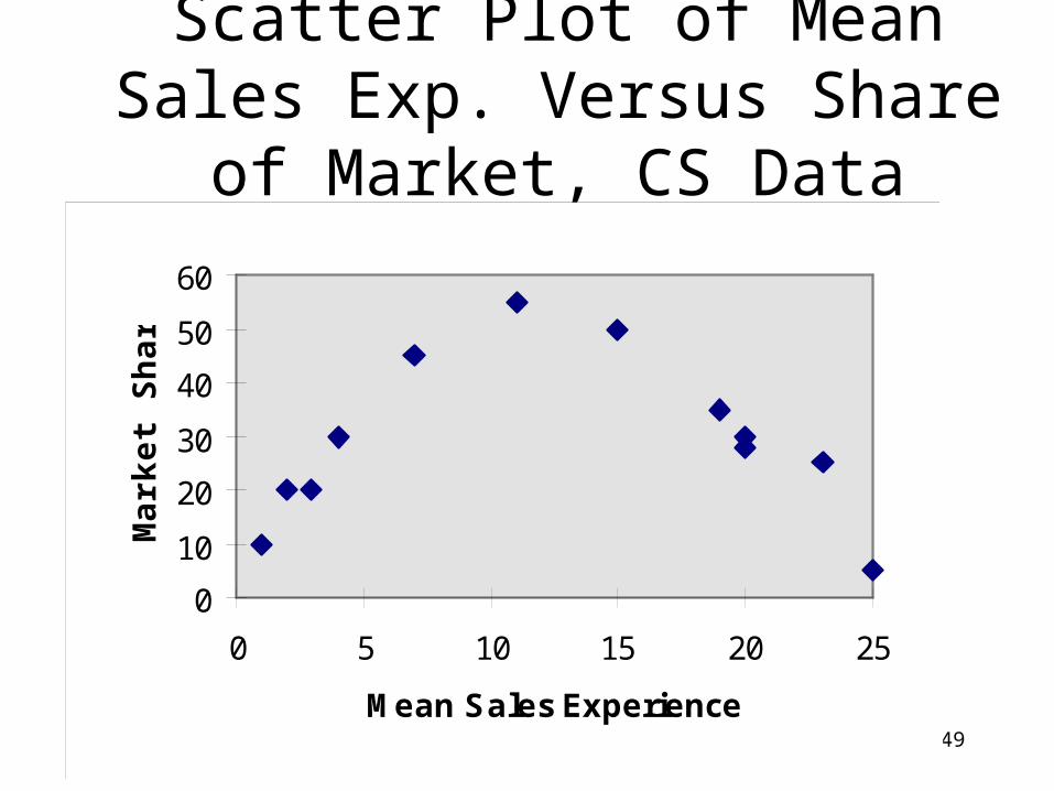
Scatter Plot of Mean Sales Exp. Versus Share of Market, CS Data

0

10

20

30

40

50

60

0 5 10 15 20 25

Mean Sales Experience

Mar

ket

Sh

are

50

Scatter Plot of Degree of Competitiveness Versus Market

Share, CS Data

0

10

20

30

40

50

60

0 0.2 0.4 0.6 0.8 1

Competitiveness

Mark

et

Sh

are

51

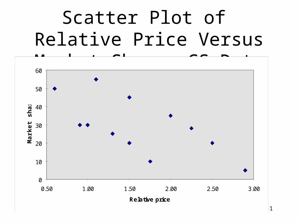
Scatter Plot of Relative Price Versus Market Share, CS Data

0

10

20

30

40

50

60

0.50 1.00 1.50 2.00 2.50 3.00

Relative price

Mar

ket

shar

e

52

Leading Predictor Variables

Does ADV (t) Affect Sales (t)? Since the Cause proceeds the Effect in time,

if we are using time-ordered data, we may need to have the effect lag the cause in time.

If advertising causes sales, does this months advertising effect this months sales or next months sales?

53

0

50

100

150

200

250

0 10 20 30 40 50

Advertising (k$)

Sal

es (

M$)

Here, we shift Adv. down 1 month

Month Adv (k$) Sales (M$)Jan 28 167Feb 23 155Mar 32 77Apr 31 179May 40 176Jun 38 228Jul 25 235

Aug 27 97Sep 29 142Oct 34 163Nov 29 167Dec 38 158

Month Lagged Adv (k$) Sales (M$)JanFeb 28 155Mar 23 77Apr 32 179May 31 176Jun 40 228Jul 38 235

Aug 25 97Sep 27 142Oct 29 163Nov 34 167Dec 29 158

0

50

100

150

200

250

0 10 20 30 40 50

Lagged Advertising (k$)

Sal

es (

M$)

54

InterpretD ata

Sum m arizeD ata

OrganizeD ata

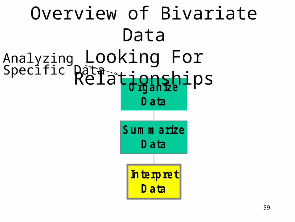
Overview of BivariateBivariate DataLooking For Relationships

AnalyzingSpecific Data

55

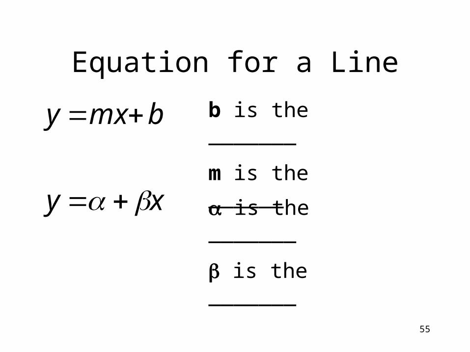
Equation for a Line

xy

bmxy

b is the _______

m is the ______

is the _______

is the _______

56

Intercept and Slope

The intercept is:

The slope is:

57

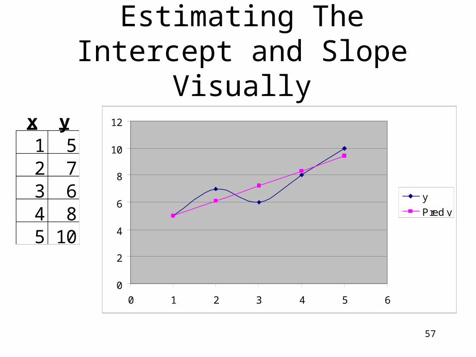
Estimating The Intercept and Slope Visually

x y1 52 73 64 85 10

0

2

4

6

8

10

12

0 1 2 3 4 5 6

y

Pred y

58

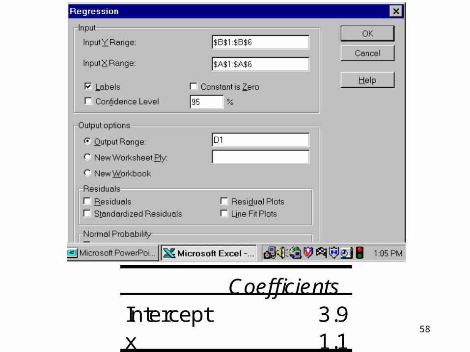
CoefficientsIntercept 3.9x 1.1

59

InterpretD ata

Sum m arizeD ata

OrganizeD ata

Overview of Bivariate DataLooking For Relationships

AnalyzingSpecific Data

60

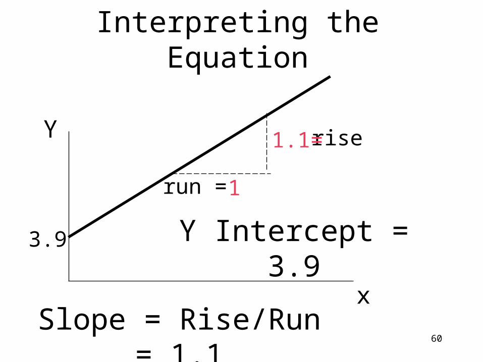
Interpreting the Equation

x

Y

3.9

rise

run =

1.1=

1

Y Intercept = 3.9

Slope = Rise/Run = 1.1

61

Multivariate AnalysisMultivariate AnalysisIs Salary Related to Months on

Job And/Or Gender?Salary Months Gender48.0 39 Male63.5 80 Male37.2 6 Male33.2 7 Male49.1 45 Male42.7 27 Male46.7 36 Male56.9 67 Male

Salary Months Gender38.5 80 Female38.8 65 Female22.5 12 Female29.7 24 Female20.4 5 Female34.0 45 Female31.2 38 Female41.1 54 Female

62

Lecture FlowD raw

Scatter P lots

63

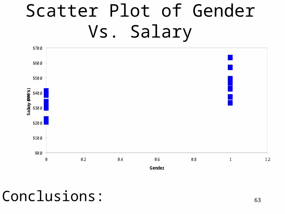
Scatter Plot of Gender Vs. Salary

Conclusions:

$0.0

$10.0

$20.0

$30.0

$40.0

$50.0

$60.0

$70.0

0 0.2 0.4 0.6 0.8 1 1.2

Gender

Sal

ary

(000

's)

64

Scatter Plot of Month Vs. Salary

Conclusions:

Scatter Plot of Month vs. Salary

$0.0

$10.0

$20.0

$30.0

$40.0

$50.0

$60.0

$70.0

0 10 20 30 40 50 60 70 80 90

Months on the Job

Sala

ry (0

00's

)

65

Purposes of Scatter Plots

Does a relation appears to exist? If so, is the relation negative or positive? What shape is the relation?

– If linear, we can apply linear regression.– If non-linear, we may apply a linear

transformation before using regression (subjects of DSc 3120 and beyond).

66

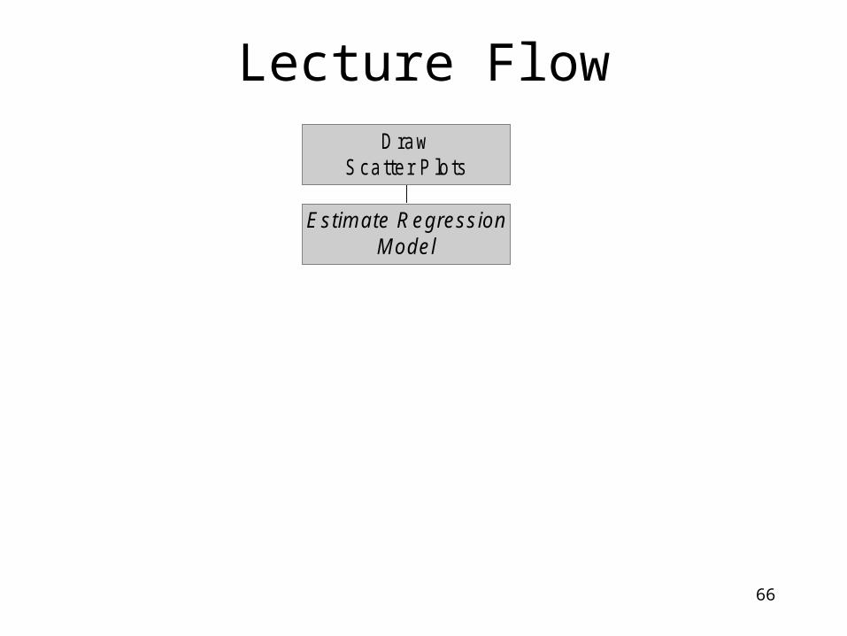
Lecture Flow

Estim ate R egressionM odel

D rawScatter P lots

67

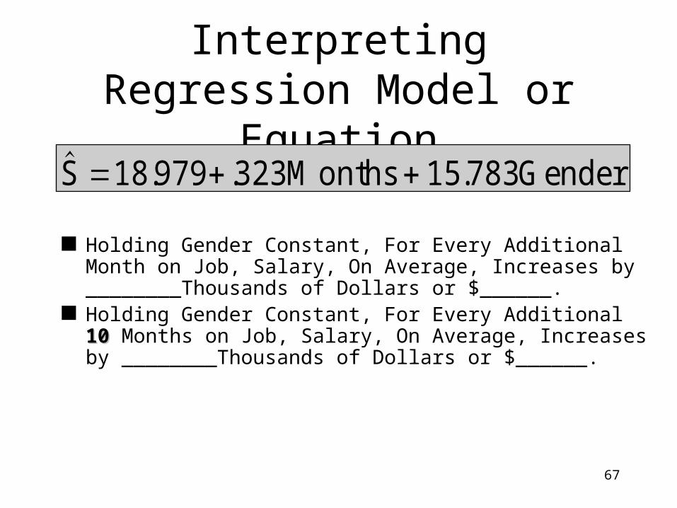
Interpreting Regression Model or Equation

. . .S M onths G ender 18 979 323 15 783

Holding Gender Constant, For Every Additional Month on Job, Salary, On Average, Increases by ________Thousands of Dollars or $______.

Holding Gender Constant, For Every Additional 1010 Months on Job, Salary, On Average, Increases by ________Thousands of Dollars or $______.

68

Estimating a Regression Model or Equation

. . .S M onths G ender 18 979 323 15 783

Holding Months on Job Constant, Males (Coded as 1), On Average, Receive _________ Thousands of Dollars More than Females.

69

Scatter Plot of Month vs. Salary

$0.0

$10.0

$20.0

$30.0

$40.0

$50.0

$60.0

$70.0

0 10 20 30 40 50 60 70 80 90

Months on the Job

Sal

ary

(000

's)

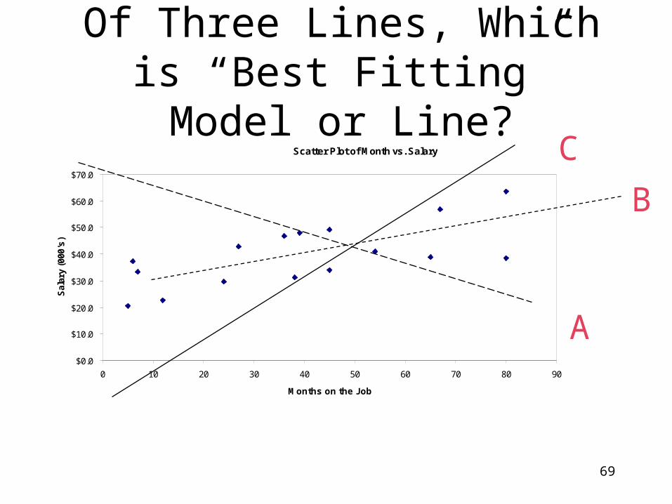
Of Three Lines, Which is “Best Fitting” Model or Line?

A

C

B

70

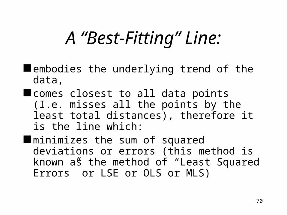
A “Best-Fitting” Line:

embodies the underlying trend of the data, comes closest to all data points (I.e. misses

all the points by the least total distances), therefore it is the line which:

minimizes the sum of squared deviations or errors (this method is known as the method of “Least Squared Errors” or LSE or OLS or MLS)

71

Minimizing The Sum of the Squared Deviations

..

..d1

d2

d3d4

BFL Minimizes d d d d12

22

32

42

Months on Job

Sal

ary

72

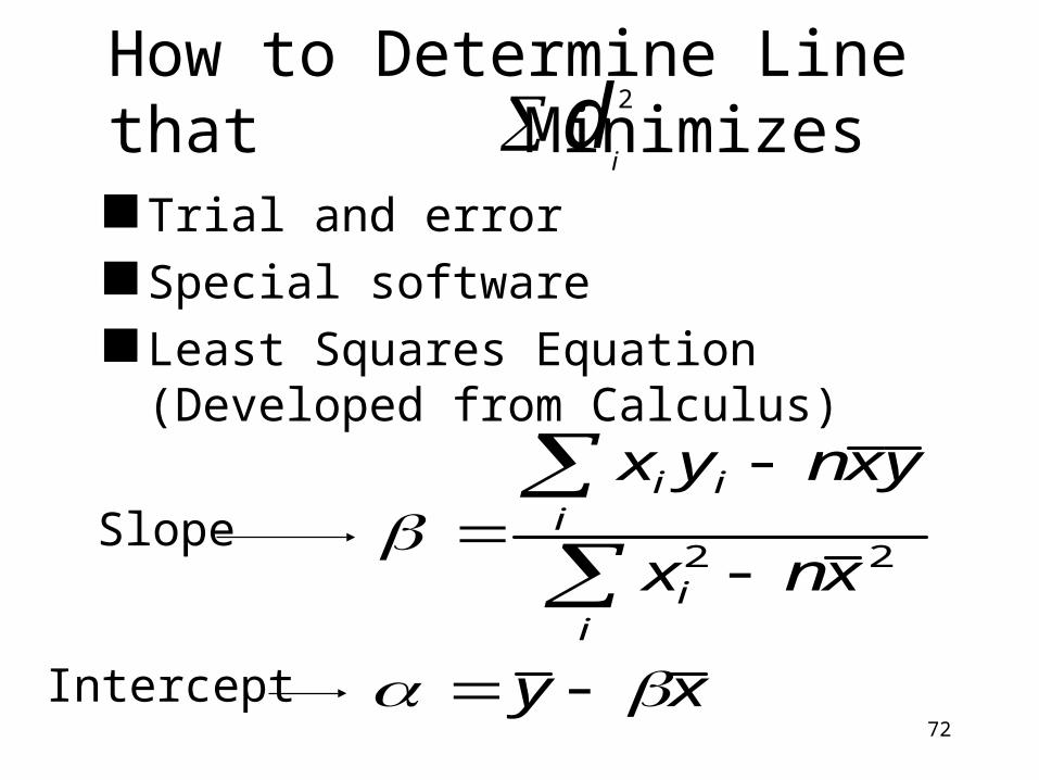
How to Determine Line that Minimizes

Trial and error Special software Least Squares Equation (Developed from

Calculus)

di

2

xy

xnx

yxnyx

ii

iii

22Slope

Intercept

73

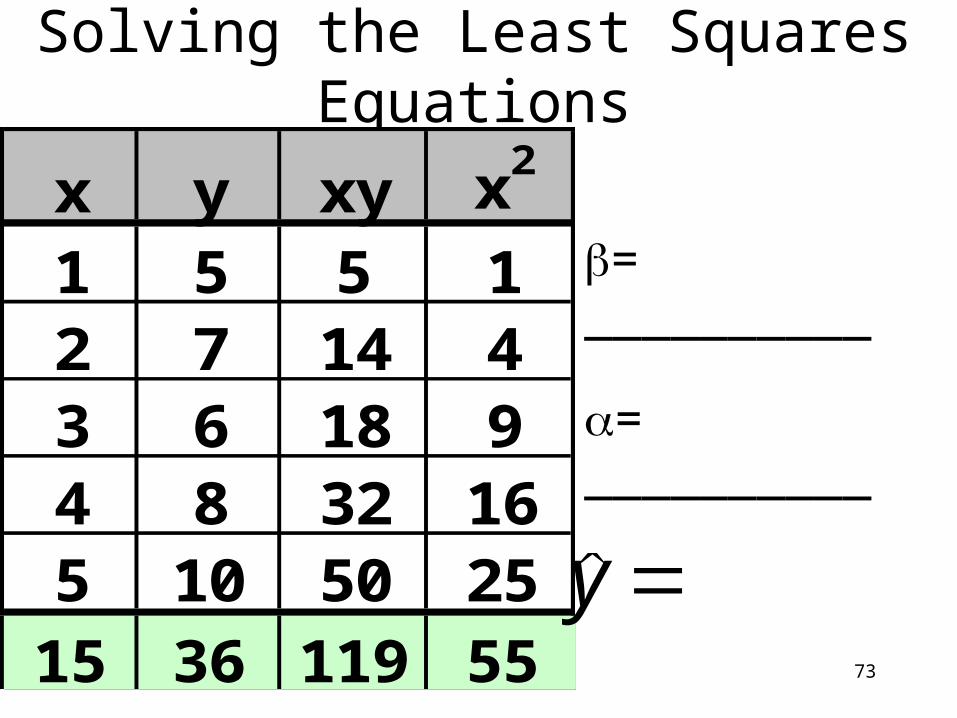
Solving the Least Squares Equations

x y xy x2

1 5 5 12 7 14 43 6 18 94 8 32 165 10 50 25

15 36 119 55

= __________

= __________

y

74

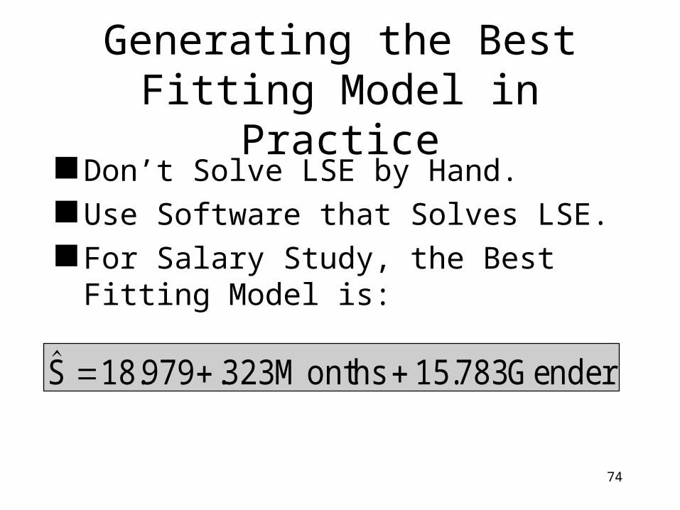
Generating the Best Fitting Model in Practice

Don’t Solve LSE by Hand. Use Software that Solves LSE. For Salary Study, the Best Fitting Model is:

. . .S M onths G ender 18 979 323 15 783

75

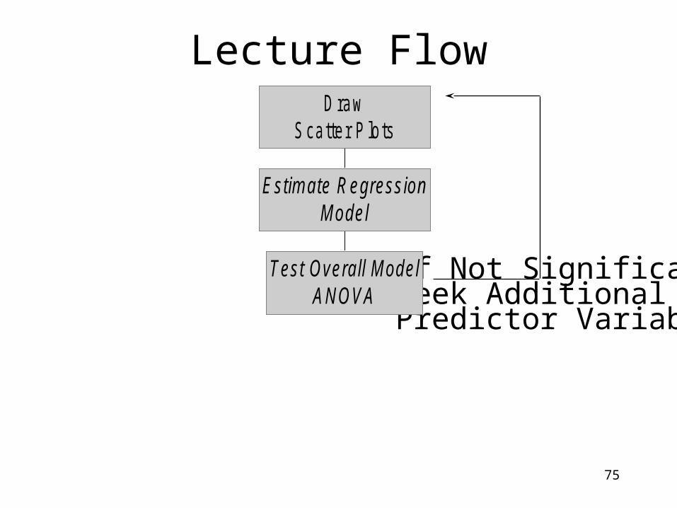
Lecture Flow

If Not Significant,Seek Additional Predictor Variables

Test Overall M odelAN OVA

Estim ate R egressionM odel

D rawScatter P lots

76

How Much Variation (Sum of Squares) Is There in Dependent

Variable??Salary48.063.537.233.249.142.746.756.9

Salary38.538.822.529.720.434.031.241.1

SST = ( )2 + ...+ ( )2

2003.129

77

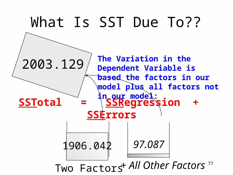
What Is SST Due To??

2003.129

Two Factors

1906.042

The Variation in the Dependent Variable is based the factors in our model plus all factors not in our model:

+ All Other Factors

97.087

SSTotal = SSRegression + SSErrors

78

ANOVA for Salary Study

Determine p-Value for F StatisticIn Excel: Significance F Value

df SS MS FRegression 2 1906 953 127.61Residual 13 97.088 7.47Total 15 2003.1

R2 = SSR/SST aka: Coefficient of Determination

79

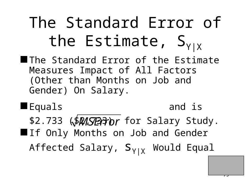
The Standard Error of the Estimate Measures Impact of All Factors (Other than Months on Job and Gender) On Salary.

Equals and is $2.733 ($2,733)

for Salary Study. If Only Months on Job and Gender Affected

Salary, sY|X Would Equal

The Standard Error of the Estimate, SY|X

MSError

80

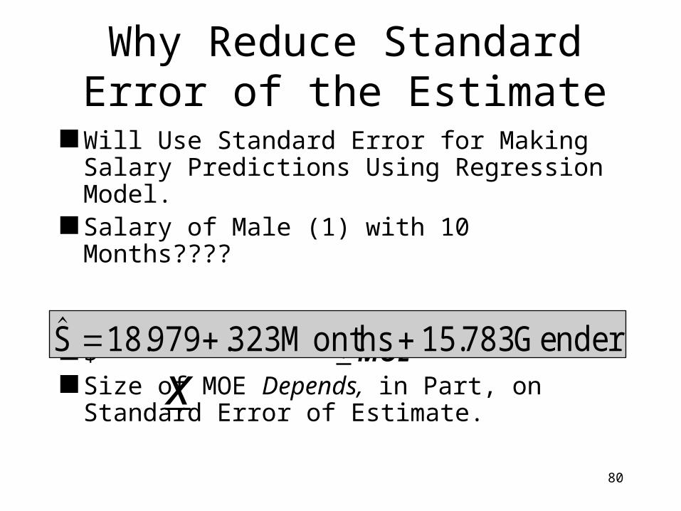
Will Use Standard Error for Making Salary Predictions Using Regression Model.

Salary of Male (1) with 10 Months????

$ + MOE Size of MOE Depends, in Part, on Standard

Error of Estimate.

Why Reduce Standard Error of the Estimate

x

. . .S M onths G ender 18 979 323 15 783

81

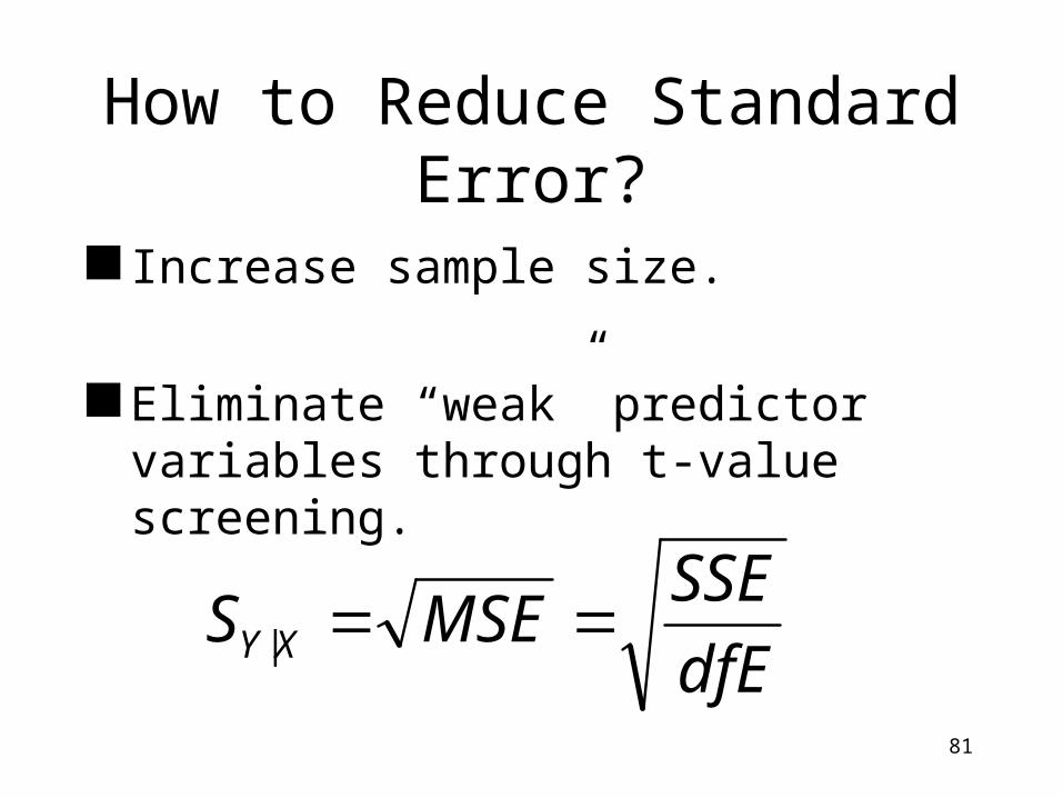
How to Reduce Standard Error?

Increase sample size.

Eliminate “weak” predictor variables through t-value screening.

dfE

SSEMSES XY |

82

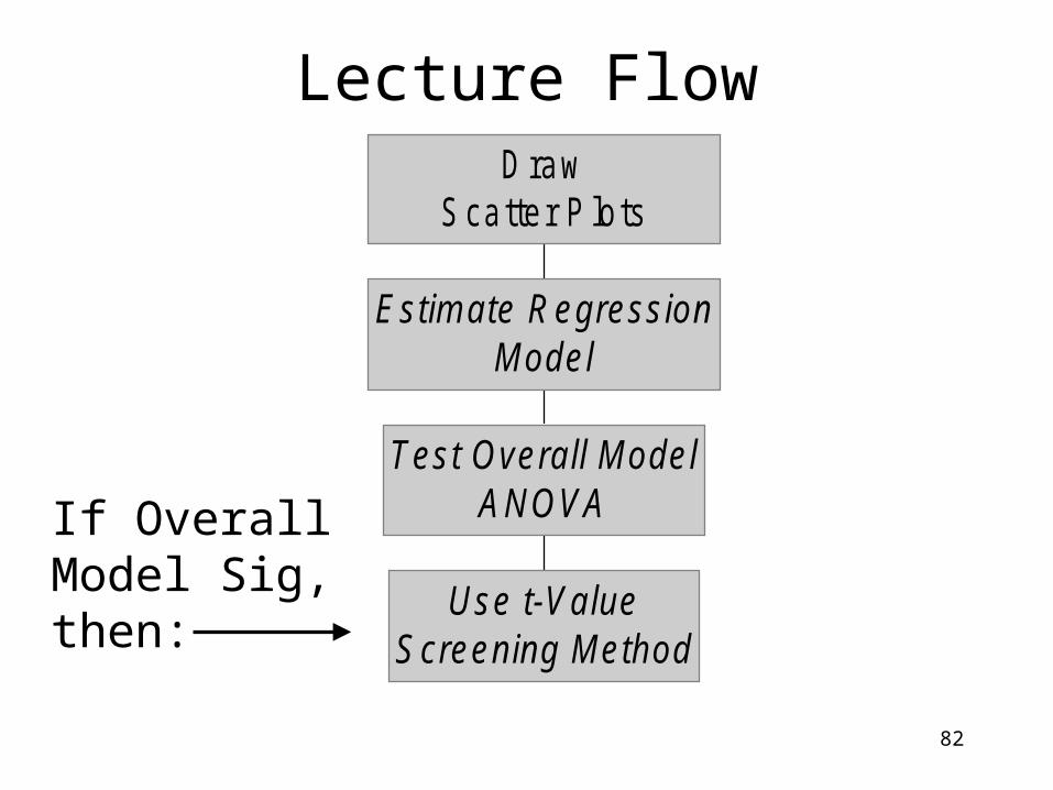
U se t-ValueScreening M ethod

Test Overall M odelAN OVA

Estim ate R egressionM odel

D rawScatter P lots

Lecture Flow

If OverallModel Sig,then:

83

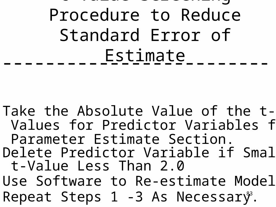
t-Value Screening Procedure to Reduce Standard Error of Estimate

1 Take the Absolute Value of the t- Values for Predictor Variables from Parameter Estimate Section.2 Delete Predictor Variable if Smallest t-Value Less Than 2.03 Use Software to Re-estimate Model.4 Repeat Steps 1 -3 As Necessary.

84

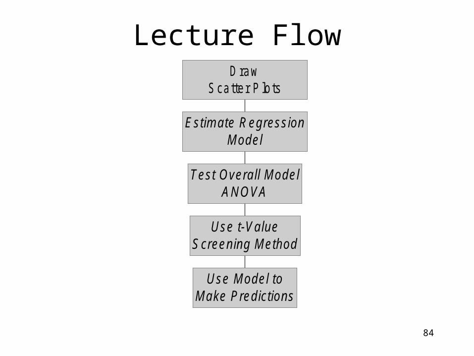
Lecture Flow

U se M odel toM ake Predictions

U se t-ValueScreening M ethod

Test Overall M odelAN OVA

Estim ate R egressionM odel

D rawScatter P lots

85

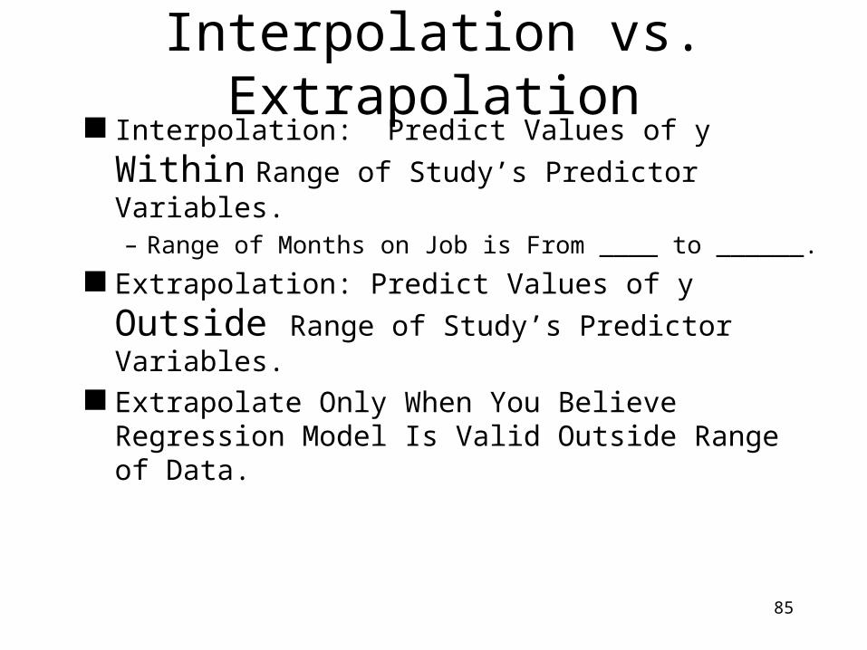
Interpolation vs. Extrapolation Interpolation: Predict Values of y Within Range

of Study’s Predictor Variables.– Range of Months on Job is From ____ to ______.

Extrapolation: Predict Values of y Outside Range of Study’s Predictor Variables.

Extrapolate Only When You Believe Regression Model Is Valid Outside Range of Data.

86

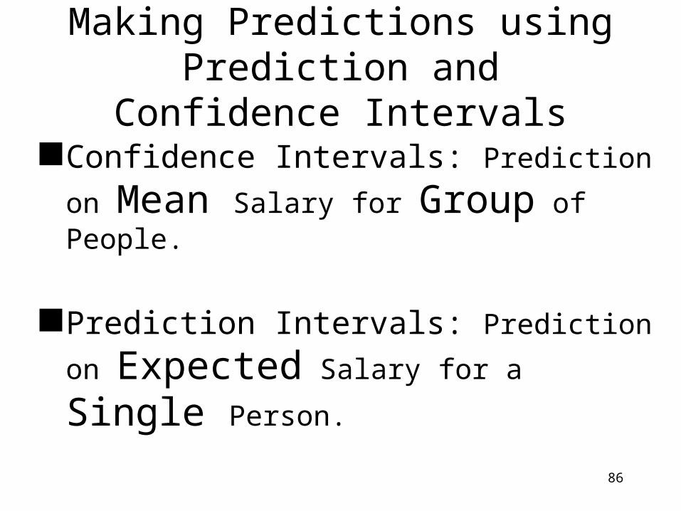
Making Predictions using Prediction and Confidence Intervals

Confidence Intervals: Prediction on Mean Salary for Group of People.

Prediction Intervals: Prediction on

Expected Salary for a Single Person.

87

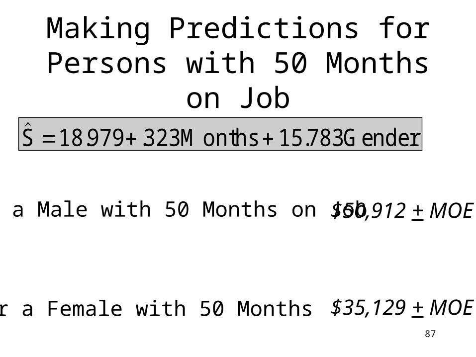
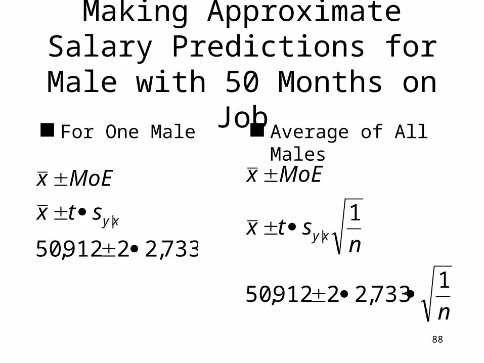
Making Predictions for Persons with 50 Months on Job

For a Male with 50 Months on Job $50,912 + MOE

For a Female with 50 Months $35,129 + MOE

. . .S M onths G ender 18 979 323 15 783

88

For One Male

Making Approximate Salary Predictions for Male with 50

Months on Job Average of All Males

733,22912,50

|

xystx

MoEx

n

nstx

MoEx

xy

1733,22912,50

1|

89

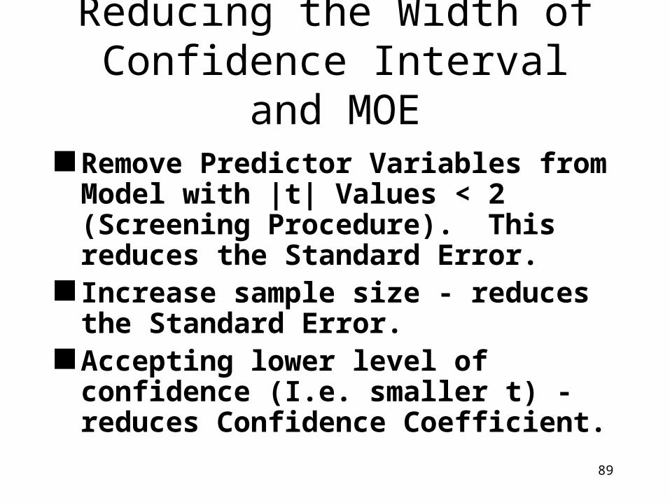
Reducing the Width of Confidence Interval and MOE

Remove Predictor Variables from Model with |t| Values < 2 (Screening Procedure). This reduces the Standard Error.

Increase sample size - reduces the Standard Error.

Accepting lower level of confidence (I.e. smaller t) - reduces Confidence Coefficient.

90

Summary of Regression

Regression Analysis Looks for Relations between variables.

What is the business application for regression?

91

Forecasting

Time Series Models

92

Forecasting Models

Budgets Sales quotas Financial pro-formas

Time series modelsCausal modelsQualitative models

93

Causal Models vs. Time Series Models

Time as a surrogate for causal factors Relate patterns in dependent variables to the

passage of time Stationary Time Series Assumption

– Data will continue to operate in the (near) future as it has in the (recent) past.

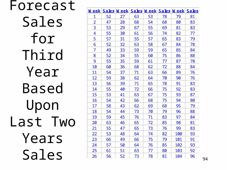
94

Forecast Sales for

Third Year Based Upon

Last Two Years Sales

Week Sales Week Sales Week Sales Week Sales1 52 27 63 53 78 79 812 47 28 68 54 68 80 833 53 29 67 55 69 81 834 55 30 61 56 74 82 775 57 31 55 57 65 83 796 52 32 63 58 67 84 787 49 33 59 59 65 85 848 52 34 55 60 75 86 889 55 35 59 61 77 87 78

10 60 36 68 62 72 88 8411 54 37 71 63 66 89 7612 59 38 62 64 70 90 7613 56 39 71 65 78 91 8314 55 40 72 66 75 92 8315 53 41 63 67 75 93 8716 54 42 66 68 75 94 8017 58 43 62 69 68 95 7918 54 44 73 70 79 96 8819 59 45 76 71 83 97 8420 63 46 65 72 85 98 8121 55 47 65 73 76 99 8322 53 48 64 74 82 100 9323 66 49 66 75 79 101 9124 57 50 64 76 85 102 9325 61 51 63 77 80 103 9226 56 52 73 78 81 104 96

95

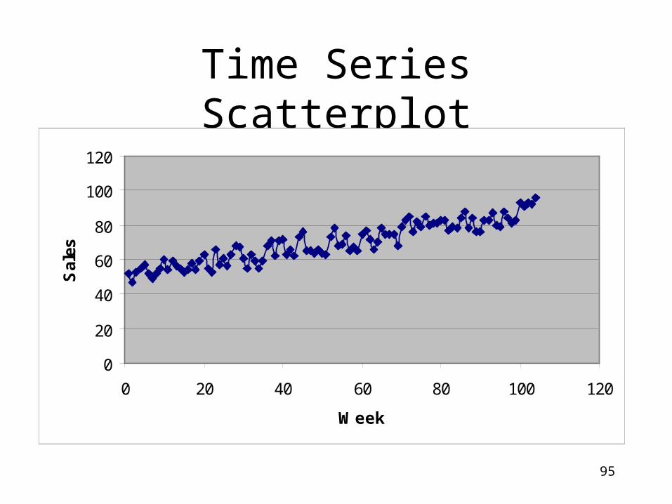
Time Series Scatterplot

0

20

40

60

80

100

120

0 20 40 60 80 100 120

Week

Sal

es

96

Naïve Model

Whatever happened recently will happen again this time.

The model is simple and flexible. Provides a baseline against which to

evaluate other models.

97

Exponential Smoothing Models

Advantages– Requires little data

– Quick and simple to compute

– Emphasizes the most up-to-date data

– Cheap

– Suitable for high-volume forecasts

Disadvantages– Simple ES always lags

trend in the data

– Double ES ignores seasonality

– Winter’s method is complex

98

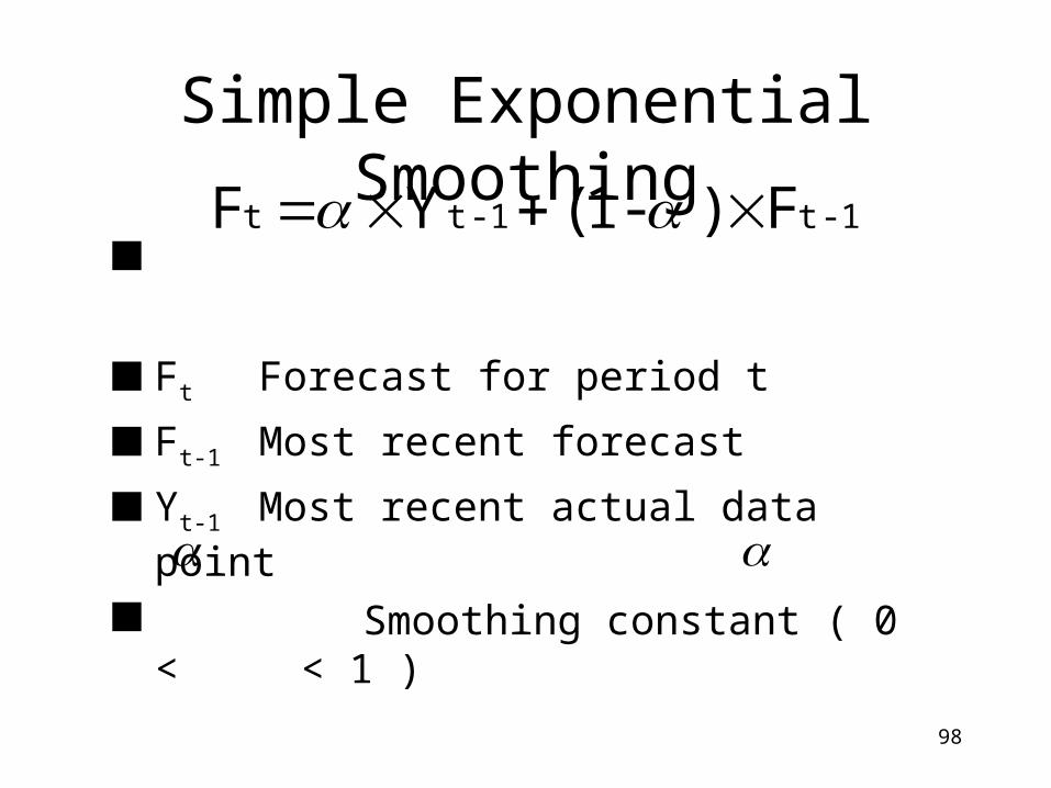
Ft Forecast for period t

Ft-1 Most recent forecast

Yt-1 Most recent actual data point

Smoothing constant ( 0 < < 1 )

Simple Exponential Smoothing1-t1-tt F ) -1 ( Y F

99

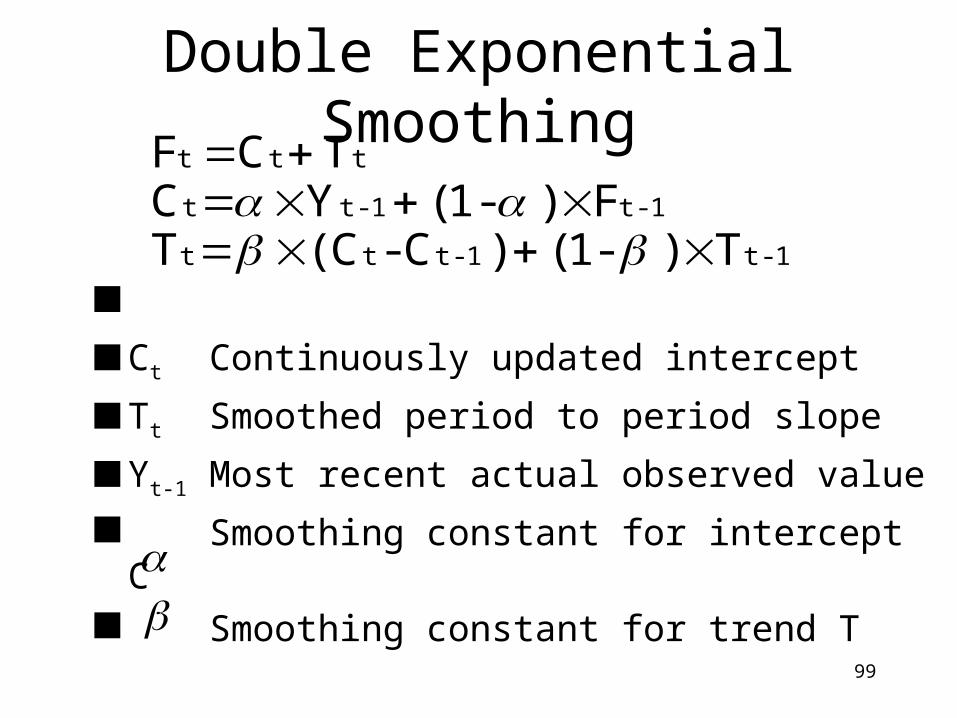
Double Exponential Smoothing

Ft Forecast for period t

Ct Continuously updated intercept

Tt Smoothed period to period slope

Yt-1 Most recent actual observed value

Smoothing constant for intercept C Smoothing constant for trend T

1-t1-ttt

1-t1-tt

ttt

T ) -1 ( ) C - C ( TF ) - 1 ( Y C

T C F

100

Winter’s Method

Adds a third smoothing constant Adds smoothed Seasonal Indices Much more complex than exponential

smoothing

101

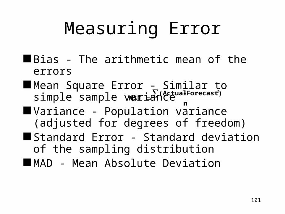
Bias - The arithmetic mean of the errors Mean Square Error - Similar to simple

sample variance Variance - Population variance (adjusted for

degrees of freedom) Standard Error - Standard deviation of the

sampling distribution MAD - Mean Absolute Deviation

Measuring Error

n

Forecast) - (Actual MSE

2

102

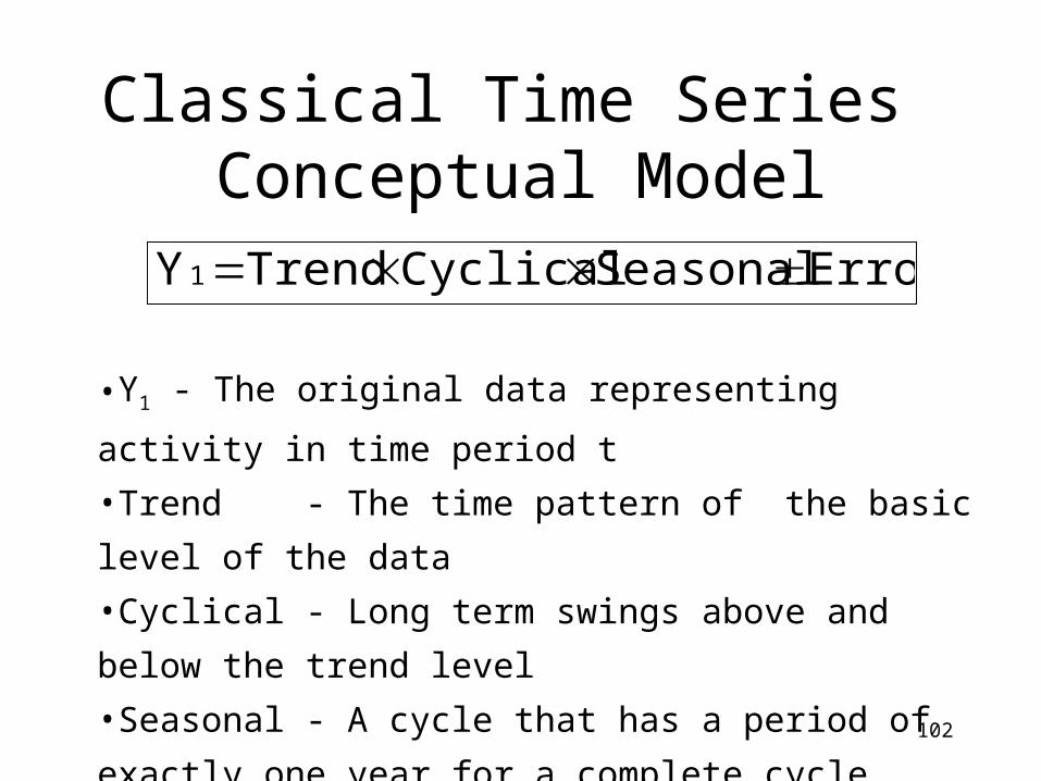
Classical Time Series Conceptual Model

Error Seasonal Cyclical Trend Y1

•Y1 - The original data representing activity in time period t

•Trend - The time pattern of the basic level of the data

•Cyclical - Long term swings above and below the trend level

•Seasonal - A cycle that has a period of exactly one year for a

complete cycle

•Error - The underlying degree of randomness or error in model

103

Trend Models

Rather than working month to month, why not fit a line through the historical data and project it into the future?

The mathematical method for calculating the best curve is called the “method of least squares.”– Minimize (Y - a - bX)2 with respect to our

choice of a and b

104

Trend Models Pros

– Can predict into the future

– Formalizes a method to minimize error term

– Can use a number of curve forms

Cons– Ignores seasonal

changes

105

Time Series Decomposition The conceptual forecasting model is:

– Y = Trend x Cyclical x Seasonal x Error

Since we cannot easily extract or predict cycles, we will assume that the trend component will capture cycles during the forecast period

Since we must live with error (we cannot predict it) our model is simplified to:– Y = Trend x Seasonal

106

Estimating Trend

Since we cannot solve for two unknowns using one equation, we must first estimate one of our values

The best estimate to work with in this case is the One Year Centered Moving Average– The advantage of CMA is that it makes no

assumptions about the underlying data and completely averages out seasonality

107

Centered Moving Average

Starting with the first datum, we average one year’s worth of observations placing the result at the center point

We continue by moving to the next datum and repeating the process until we no longer have a complete year to average

108

Centered Moving Average

The initial average lies between the middle values (quarters or months)

To get the centered moving average, we average the two values on either side to get the CMA

NOTE: In averaging one year of data, we lose the first and last six months

109

Raw Seasonal Ratios

Now that we have an estimate for trend, we can solve our general model for seasonality– Season = Y / Trend

We use this formula to calculate the Raw Seasonal Ratio

The Raw Seasonal Ratio is used to calculate the Seasonal Index

110

Seasonal Index

To calculate the Seasonal Index for each period, average the raw ratios for each similar period then center the averages about 1

Divide each season’s average by the overall (grand) average to force the average of all Seasonal Indices to equal 1

111

Deseasonalized Data

Going back to the conceptual model, solve for trend:– Trend = Y / Season

This eliminates seasonal variation and isolates the trend

Now use the Least Squares method to compute the Trend

112

Forecast

Now that we have the Seasonal Indices and Trend, we can reseasonalize the data and generate the forecast– Y = Trend x Season

113

Deciding Between Forecasting Models & Methods

Look at the errors over the backcast or for a holdout sample:– Bias near zero– MAD, MAPE, & Std Error near Zero– Coefficient of Determination (R2) near unity.

How well does it perform in repeated uses and during validation with different data.

114

Deciding Between Forecasting Models & Methods

What if several models are approximately “equally good”?– The Rule of Parsimony (or using Occam’s

Razor), we would choose the simplest, easiest, most cost effective model that meets our needs.